| Issue |
A&A
Volume 703, November 2025
|
|
|---|---|---|
| Article Number | A129 | |
| Number of page(s) | 20 | |
| Section | Extragalactic astronomy | |
| DOI | https://doi.org/10.1051/0004-6361/202556085 | |
| Published online | 19 November 2025 | |
Brightest group galaxies in COSMOS-Web: Evolution of the size-mass relation since z = 3.7
1
Department of Computer Science, Aalto University, PO Box 15400 Espoo FI-00076, Finland
2
Department of Physics, University of Helsinki, P. O. Box 64 FI-00014 Helsinki, Finland
3
Laboratory for Multiwavelength Astrophysics, School of Physics and Astronomy, Rochester Institute of Technology, 84 Lomb Memorial Drive, Rochester, NY 14623, USA
4
University of Bologna – Department of Physics and Astronomy “Augusto Righi” (DIFA), Via Gobetti 93/2 I-40129, Bologna, Italy
5
INAF – Osservatorio di Astrofisica e Scienza dello Spazio di Bologna, Via Gobetti 93/3 40129 Bologna, Italy
6
Zentrum für Astronomie, Universität Heidelberg, Philosophenweg 12 69120 Heidelberg, Germany
7
Institute for Advanced Studies in Basic Sciences (IASBS), 444 Prof. Yousef Sobouti Blvd., Zanjan 45137-66731, Iran
8
Aix Marseille Univ, CNRS, LAM, Laboratoire d’Astrophysique de Marseille, Marseille, France
9
Department of Physics and Astronomy, University of Victoria, BC V8X 4M6 Canada
10
Infosys Visiting Chair Professor, Indian Institute of Science, Bangalore 560012, India
11
Department of Physics, University of California, Santa Barbara, Santa Barbara, CA 93106, USA
12
The University of Texas at Austin, 2515 Speedway Blvd Stop C1400, Austin, TX 78712, USA
13
Cosmic Dawn Center (DAWN), Denmark
14
Department of Physics, University of Hawaii, Hilo, 200 W Kawili St, Hilo, HI 96720, USA
15
Caltech/IPAC, MS 314-6, 1200 E. California Blvd., Pasadena, CA 91125, USA
16
Université Paris-Saclay, Université Paris Cité, CEA, CNRS, AIM, 91191 Gif-sur-Yvette, France
17
Institute for Computational Cosmology, Department of Physics, Durham University, South Road, Durham DH1 3LE, United Kingdom
18
Deutsches Zentrum für Astrophysik, Postplatz 1 02826 Görlitz, Germany
19
TU Dresden, Institute of Nuclear and Particle Physics, 01062, Dresden, Germany; DESY, Notkestrasse 85 22607 Hamburg, Germany
20
Department of Physics and Astronomy, University of California, Riverside, 900 University Avenue, Riverside, CA 92521, USA
21
Centre for Astrophysics Research, University of Hertfordshire, Hatfield AL10 9AB, UK
22
Department of Physics and Astronomy, University of Kentucky, 505 Rose Street, Lexington, KY 40506, USA
23
Space Telescope Science Institute, 3700 San Martin Drive, Baltimore, MD 21218, USA
24
Institut d’Astrophysique de Paris, UMR 7095, CNRS, and Sorbonne Université, 98 bis boulevard Arago 75014 Paris, France
25
Purple Mountain Observatory, Chinese Academy of Sciences, 10 Yuanhua Road, Nanjing 210023, China
26
DTU-Space, Technical University of Denmark, Elektrovej 327 2800 Kgs. Lyngby, Denmark
27
ITP, Universität Heidelberg, Philosophenweg 16 69120 Heidelberg, Germany
28
INFN – Sezione di Bologna, Viale Berti Pichat 6/2 40127 Bologna, Italy
29
School of Physics and Astronomy, University of Southampton, Highfield SO17 1BJ, UK
30
Department of Astronomy and Astrophysics, University of California, Santa Cruz, 1156 High Street, Santa Cruz, CA 95064, USA
31
National Research Institute of Astronomy and Geophysics (NRIAG), Cairo, Egypt
32
EPFL Laboratory of Astrophysics (LASTRO), Observatoire de Sauverny, CH – 1290 Versoix, Switzerland
33
Jet Propulsion Laboratory, California Institute of Technology, 4800 Oak Grove Drive, Pasadena, CA 91001, USA
34
Astronomy Department, California Institute of Technology, 1200 E. California Blvd, Pasadena, CA 91125, USA
35
Niels Bohr Institute, University of Copenhagen, Jagtvej 128 2200 Copenhagen, Denmark
36
University of Geneva, 24 rue du Général-Dufour 1211 Genéve 4, Switzerland
37
Institute for Astronomy, University of Hawai’i at Manoa, 2680 Woodlawn Drive, Honolulu, HI 96822, USA
38
Thüringer Landessternwarte, Sternwarte 5 07778 Tautenburg, Germany
39
Helmholtz-Institut für Strahlen-und Kernphysik (HISKP), Universität Bonn, Nussallee 14-16 D-53115, Bonn, Germany
40
INAF-Osservatorio Astronomico di Trieste, Via G.B. Tiepolo 11 34143 Trieste, Italy
41
IFPU: Institute for Fundamental Physics of the Universe, Via Beirut, 2 34151, Italy
⋆ Corresponding author: This email address is being protected from spambots. You need JavaScript enabled to view it.
; This email address is being protected from spambots. You need JavaScript enabled to view it.
Received:
24
June
2025
Accepted:
5
September
2025
Abstract
We present the first comprehensive study of the structural evolution of brightest group galaxies (BGGs) from redshift z ≃ 0.08 to z = 3.7 using the James Webb Space Telescope’s 255-hour COSMOS-Web program. This survey provides deep NIRCam imaging in four filters (F115W, F150W, F277W, and F444W) in ∼ 0.54 deg2, allowing robust size and morphological measurements for ∼ 1700 BGGs spanning ∼ 12 Gyr of cosmic history. High-resolution imaging enables consistent measurement of galaxy sizes in the rest-frame optical (red to near-infrared; ∼6000–8000 Å) across cosmic time through redshift-dependent filter selection. We classified BGGs as star-forming and quiescent using both rest-frame NUV–r–J colors and redshift-dependent specific star formation rate (sSFR) thresholds. Our structural analysis reveals that quiescent BGGs are systematically more compact than their star-forming counterparts across all redshifts, exhibiting steeper size–mass slopes (αQG ∼ 0.6–1.2 vs. αSF ∼ 0.0–0.3). The effective radius evolves as Re ∝ (1+z)−α, with α = 0.96 ± 0.07 for star-forming BGGs and α = 1.24 ± 0.09 for quiescent BGGs, indicating stronger size growth in quenched systems. The corresponding growth factor at fixed stellar mass (log M∗ = 10.7) from z = 3.7 to z = 0.08 is ∼ 4.4 for star-forming and ∼ 6.6 for quiescent BGGs. The intrinsic scatter in the size–mass relation increases toward higher redshift for both populations, reaching ∼ 0.3–0.4 dex at z > 2, reflecting greater structural diversity in the early universe. Compared to field galaxies, BGGs show systematically smaller sizes at fixed stellar mass, particularly among quiescent systems, highlighting environmental effects on galaxy structure. We further compare the evolution of the quiescent fraction, the Sérsic index, and ellipticity with those of field galaxies, finding consistent trends that reinforce our main conclusions. These results establish the foundation for understanding how group-scale environments shape the structural evolution of central galaxies and provide crucial constraints for models of galaxy formation in intermediate-mass dark matter halos.
Key words: galaxies: clusters: general / galaxies: evolution / galaxies: groups: general / galaxies: high-redshift / galaxies: star formation / galaxies: structure
© The Authors 2025
 Open Access article, published by EDP Sciences, under the terms of the Creative Commons Attribution License (https://creativecommons.org/licenses/by/4.0), which permits unrestricted use, distribution, and reproduction in any medium, provided the original work is properly cited.
This article is published in open access under the Subscribe to Open model. This email address is being protected from spambots. You need JavaScript enabled to view it. to support open access publication.
1. Introduction
Understanding the structural evolution of galaxies across cosmic time is fundamental to unraveling the processes that govern galaxy formation and transformation. Although extensive work has characterized the size evolution of field galaxies Williams et al. 2010; Belli et al. 2015 and brightest cluster galaxies (BCGs) in the most massive halos Stott et al. 2011; Yang et al. 2024, the structural properties of galaxies in intermediate environments remain relatively unexplored, particularly at high redshift.
Galaxy groups, with halo masses 1013 ≲ Mhalo ≲ 1014 M⊙, represent a crucial and abundant component of the cosmic web, contributing ∼30%–50% of the total mass budget in the Universe Cui 2024; Pillepich 2021; Bocquet et al. 2019. Brightest group galaxies (BGGs), the most massive and luminous galaxies residing at the centers of these groups, serve as unique laboratories for studying galaxy evolution in intermediate-mass environments. Unlike BCGs in massive clusters or isolated central galaxies, BGGs experience a distinct regime of environmental effects, including moderate merger rates, intermediate gas densities, and gradual assembly histories Gozaliasl et al. 2016, 2018, 2020. The structural evolution of massive galaxies is governed by several competing physical processes. Star-forming galaxies (SFGs) grow primarily through gas accretion and inside-out assembly Mo et al. 1998; Oesch et al. 2010; Mosleh et al. 2012, leading to relatively shallow size–mass scaling relations. In contrast, quiescent galaxies (QGs) exhibit more compact morphologies and steeper structural scaling, consistent with formation through dissipative collapse followed by gas-poor mergers Toft et al. 2007; Belli et al. 2014; Kriek et al. 2009. The transition between these regimes is marked by a critical stellar mass scale near log(M⋆/M⊙)∼11, above which dry mergers become increasingly important for size growth Peng et al. 2010; Poggianti et al. 2013. Observations of massive galaxies reveal substantial size evolution, with effective radii increasing by factors of ∼2–3 from z = 2 to the present Williams et al. 2010; Belli et al. 2015. However, this evolution is not uniform across galaxy types or environments. Early-type galaxies show steeper size evolution (Reff ∝ (1 + z)−1.48) compared to late-types (Reff ∝ (1 + z)−0.75), reflecting different assembly histories and quenching mechanisms van der Wel et al. 2014. Similarly, ultra-massive galaxies (log M*/M⊙ > 11.4) exhibit remarkably uniform size evolution across cosmic time, suggesting efficient post-quenching growth through minor mergers Faisst et al. 2017.
The role of environment in shaping galaxy structure is well established in the local Universe, where central galaxies in groups and clusters are systematically more compact than field galaxies of similar mass van der Burg et al. 2014; Kravtsov 2018. However, the redshift evolution of these environmental effects remains poorly constrained, particularly for BGGs, due to the challenges of identifying group-scale structures at high redshift with sufficient statistical power.
Recent work by Yang et al. 2025 used the COSMOS-Web survey – part of the Cosmic Evolution Survey (COSMOS; Scoville et al. 2007) – to measure rest-frame optical sizes of galaxies from z = 2 to z = 10, revealing that SFGs maintain nearly constant size–mass slopes and surface density relations, while quiescent systems show steeper structural scaling and a clear compactness threshold. These findings provide a crucial reference for understanding how environmental effects modify the general trends observed in field galaxies.
The James Webb Space Telescope (JWST) has revolutionized our ability to study galaxy structure at high redshift, providing unprecedented resolution and sensitivity in the near-infrared. The COSMOS-Web survey, the largest JWST program in Cycle 1 Casey et al. 2023, offers an ideal dataset for investigating BGG structural evolution by combining deep, high-resolution imaging with the largest and most complete catalog of galaxy groups at z > 1 assembled to date Toni et al. 2025.
In this study, we present the first comprehensive analysis of BGG structural evolution from z = 0.08 to z = 3.7 using COSMOS-Web NIRCam observations. We investigate the size–mass relation, quantify size growth at fixed stellar mass, and characterize the intrinsic scatter and its evolution across cosmic time. By comparing BGGs to field galaxy populations, we constrain the role of group-scale environments in shaping galaxy structure and provide essential observational benchmarks for theoretical models of galaxy formation.
This paper is organized as follows. In Section 2, we describe the COSMOS-Web survey, the group catalog, and the BGG selection methodology. Section 3 outlines our structural measurement techniques and galaxy classification scheme. Section 4 presents our main results on size–mass scaling, size evolution, and structural distributions. Section 5 discusses the implications for galaxy formation models and compares our findings with previous work. Finally, we summarize our conclusions.
Throughout this paper, we adopt a flat ΛCDM cosmology with parameters H0 = 67.66 km s−1 Mpc−1, Ωm, 0 = 0.30966, and ΩΛ, 0 = 0.68884, consistent with Planck 2018 Aghanim et al. 2020. All magnitudes are expressed in the AB system Oke 1974.
2. Galaxy and group dataset
2.1. The COSMOS-Web survey
The COSMOS-Web survey is the largest JWST Cycle 1 program, covering 0.54 deg2 with NIRCam in four filters (F115W, F150W, F277W, and F444W) and 0.19 deg2 with MIRI F770W Casey et al. 2023. NIRCam achieves 5σ depths of 26.6–27.3 mag (F115W), 26.9–27.7 mag (F150W), 27.5–28.2 mag (F277W), and 27.5–28.2 mag (F444W) within 0.15″apertures. Observations span January 2023 to May 2024. We used high-resolution 30 mas mosaics for structural measurements. Data reduction is detailed in Franco et al. 2024, 2025; Harish et al. 2025.
2.2. COSMOS-Web photometric catalog
We performed photometric extraction using SOURCEXTRACTOR++ (SE++) Bertin et al. 2020; Kümmel et al. 2020 with parametric Sérsic fitting across 33 filters. An alternative structural catalog Yang et al. 2025 provided independent Sérsic fits in each NIRCam band for rest-frame analysis. We derived spectral energy distributions (SEDs) and physical parameters from LEPHARE template fitting Arnouts et al. 2002; Ilbert et al. 2006, using Bruzual & Charlot 2003 stellar population models with various star formation histories and dust laws Calzetti et al. 2000; Salim et al. 2018. Photometric redshifts achieve σNMAD ≈ 0.013 for F444W < 25.0 mag when compared to spectroscopic redshifts Khostovan et al. 2025. Validation of the stellar mass through CIGALE comparisons Boquien et al. 2019; Shuntov et al. 2024 confirms the consistency between methods. The full details on COSMOS2025 and the photometric catalog of galaxies can be found in Franco et al. 2025.
2.3. Galaxy groups and BGG selection
We used the COSMOS-Web galaxy group catalog Toni et al. 2025, the largest JWST-based group sample covering 0.54 deg2 (0.45 deg2 effective) from z = 0.08 to z = 3.7. Groups were detected using the AMICO (Adaptive Matched Identifier of Clustered Objects) algorithm Bellagamba et al. 2018; Maturi et al. 2019, applied to 389,248 high-quality galaxies, yielding 1678 groups with S/Nnocl > 6.0. Purity exceeded 80% for S/Nnocl > 9.5 based on SinFoniA mock validation Maturi et al. 2023. Over 500 groups have spectroscopic confirmation Khostovan et al. 2025. To identify BGGs, we introduced a hybrid selection method that employed stellar mass and luminosity criteria within 250–500 kpc apertures from group centers. This approach addresses spatial offsets in low-mass systems and starburst contamination in luminosity-based selections. The method first identifies both the highest stellar mass and the brightest (F150W band) galaxy separately within 250–500 kpc apertures from group centers. It applies a tiered decision tree: (1) selects the mass-dominant galaxy if stellar mass exceeds the luminosity-selected candidate by ≥0.1 dex; (2) chooses the luminosity-dominant galaxy if brighter by an equivalent margin; (3) defaults to the brighter galaxy when mass differences are < 0.1 dex. We restricted the analysis to groups with λ⋆ > 4 (see Fig. 1) to ensure completeness. The hybrid method achieves 77.1% agreement with mass-based and 71.6% with luminosity-based selections, compared to 48.7% agreement between individual methods alone. This yielded a robust sample of BGGs for structural analysis. Detailed selection methodology and validation are presented in the Appendix A.
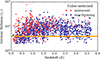 |
Fig. 1. Intrinsic richness, λ*, of detected groups and its trend with redshift. Bright group galaxies (BGGs), classified as quiescent or star-forming based on color-color criteria, are shown with red and blue points, respectively. The dashed horizontal orange line indicates the λ* limit applied in this study. |
2.4. Classification of BGGs: Star-forming and quiescent
To investigate the evolutionary trends of BGGs, we classified them into SFGs and QGs using a combination of rest-frame color-color selection and sSFR thresholds. This dual approach allowed for a more robust classification by accounting for both photometric and physical star formation indicators. To investigate the structural and evolutionary differences between star-forming and quiescent BGGs, we classified our sample using three complementary approaches: (i) a rest-frame color–color diagram, (ii) a redshift-dependent sSFR threshold, and (iii) an integrated method combining both criteria. This multitiered classification ensures robustness against contamination by dusty SFGs and transitional systems.
2.4.1. Color–color classification: NUV–r–J diagram
We employed the rest-frame MNUV − Mr versus Mr − MJ (NUV–r–J) color–color diagram to separate passive from active systems. Following Ilbert et al. 2013, a galaxy is considered quiescent if it satisfies both of the following conditions:
 (1)
(1)
This method effectively distinguishes red, passively evolving systems from those dominated by ongoing star formation or dust-reddened emission. The classification is calibrated and most reliable within the redshift range 0 < z < 4, where the photometric bands and derived rest-frame colors are well constrained by the available multiwavelength data.
2.4.2. Specific star formation rate (sSFR) selection: Redshift-dependent threshold
To complement color-color-based classification and mitigate contamination from dust-obscured star-forming galaxies, we applied a redshift-dependent threshold on the sSFR, following the formalism of Pacifici et al. 2016. A BGG is classified as quiescent if:
 (2)
(2)
where  is given in yr−1, and tobs(z) represents the age of the Universe at the galaxy’s redshift, in Gyr. This threshold evolves with cosmic time and reflects the declining global star formation rate, providing a more physically motivated and redshift-aware definition of quiescence. Figure 2 illustrates the evolution of the sSFR threshold as a function of cosmic time (bottom axis) and redshift (top axis), based on the adopted ΛCDM cosmology. The threshold becomes more stringent at earlier epochs, reflecting the higher star formation activity of galaxies in the early Universe. At later times (lower redshifts), the sSFR threshold declines steadily, consistent with the cosmic decline in star formation rate density.
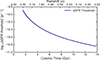 |
Fig. 2. Redshift-dependent sSFR threshold used to classify BGGs as quiescent, defined as log10(sSFR) < log10(0.2/tobs). The bottom x axis shows cosmic time in Gyr, while the top x axis shows the corresponding redshift. The threshold decreases smoothly from early to late cosmic epochs, tracing the decline in global star formation efficiency. |
2.4.3. Hybrid classification: Color-color and sSFR criteria
Although the NUV–r–J diagram and the sSFR threshold each provide effective classification schemes, discrepancies can arise due to photometric uncertainties or atypical dust attenuation. Therefore, we define a final high-confidence classification based on consensus.
-
Quiescent BGGs (QGs) must satisfy both the color–color and sSFR quiescent criteria.
-
Star-Forming BGGs (SFGs) must fail both criteria.
-
BGGs meeting only one criterion are excluded from the final classification to avoid ambiguity.
This conservative approach ensures a clean division between star-forming and passive systems and improves the reliability of subsequent evolutionary analyses.
2.4.4. Final classified sample
Applying the combined classification to our stellar-mass-selected sample of BGGs (log M*/M⊙ > 9 and λstar > 4), we obtained a clean and conservative division into star-forming and quiescent systems across the redshift interval 0.08 < z < 3.7. This refined classification serves as the basis for our structural analysis in subsequent sections. It allows us to explore the redshift evolution of the size–mass relation separately for SFGs and QGs, while minimizing the impact of classification uncertainties.
Figure 3 presents the distribution of BGGs in rest-frame NUV–r versus r–J color space across six redshift bins from z = 0.0 to z = 3.7.0. Each galaxy is color-coded by its log10(sSFR), providing insight into its recent star formation activity. The magenta lines indicate the quiescent region, as defined by the NUV–r–J criteria.
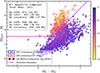 |
Fig. 3. Rest-frame NUV–r versus r–J color–color diagram for all BGGs combined across the full redshift range z = 0 to z = 4. Points are color-coded by their log10(sSFR/yr−1). Magenta lines delineate the quiescent region defined by |

Each panel annotates the number of BGGs classified as quiescent or star-forming according to the three distinct methods.
The open red and blue squares in each panel mark the BGGs that meet both quiescent and star-forming definitions, respectively, and represent the clean sample used for subsequent analysis. We also performed the analysis using both color-color and redshift-dependent sSFR thresholds.
As shown in the panels, at higher redshifts (z ≳ 2), the majority of BGGs reside in the star-forming region of the diagram and exhibit high sSFRs. Toward lower redshifts (z ≲ 1.5), an increasing number of BGGs populate the quiescent region, indicating a buildup of massive, quenched systems over cosmic time. The combined classification method (color + sSFR) filters out transitional or dusty systems, ensuring a more secure division of BGGs into star-forming and quiescent types.
The total number of BGGs identified as star-forming or quiescent in each redshift bin is shown in Table B.1.
This classification framework ensures a high-purity sample of star-forming and quiescent BGGs, free from potential contamination by dusty starbursts or intermediate systems. The robust selection improves the reliability of subsequent structural analyses, such as the size-mass relation and the size evolution presented in Sections 4.1 and 4.3. To ensure that our results were not affected by incompleteness, we applied a stellar mass cut of M⋆ ≥ 1010 M⊙, which guarantees mass completeness for both quiescent and star-forming galaxies up to z = 3.75. This limit was derived using the method of Pozzetti et al. 2010, in which the 30% faintest galaxies in each redshift bin were used to estimate the limiting stellar mass, Mresc, by scaling their F444W magnitudes to the survey’s magnitude limit (27.4 mag). The completeness limit corresponded to the 95th percentile of the Mresc distribution in each bin. We verified that adopting the fixed cut of 1010 M⊙ was more conservative than the calculated limits across all bins.
All key results remain unchanged when the analysis is restricted to this mass-complete subsample. The quiescent fraction as a function of redshift for the mass-complete sample is presented in Appendix F.
3. Structural measurements of BGGs
3.1. Sizes of BGGs
To quantify the structural properties of BGGs, we performed two-dimensional Sérsic profile fitting on JWST/NIRCam imaging. For a comprehensive description of the size measurement pipeline and validation, we refer the reader to Yang et al. 2025, who conducted a systematic structural analysis of galaxies in the COSMOS-Web survey. Here we summarize the most relevant aspects of their methodology, which we adopted for this work.
We modeled the surface brightness distribution of each galaxy using a single-component Sérsic function Sersic 1968:
![Mathematical equation: $$ \begin{aligned} I(r) = I_0 \exp \left[ -b_n \left(\frac{r}{R_e}\right)^{1/n} - 1 \right], \end{aligned} $$](/articles/aa/full_html/2025/11/aa56085-25/aa56085-25-eq6.gif) (3)
(3)
where I0 is the central surface brightness, Re is the effective (half-light) radius, n is the Sérsic index that defines the concentration of the light profile, and bn is a normalization constant dependent on n. The elliptical radius was defined as  , where q is the axis ratio of the light distribution.
We adopted measurements from the COSMOS-Web structural catalog generated with the Galight software package Ding et al. 2020, built on the Lenstronomy lens modeling framework Birrer et al. 2021. This pipeline fits galaxy light profiles while simultaneously modeling neighboring objects and incorporating accurate point spread function (PSF) convolution.
Following Yang et al. 2025, we constructed the PSF for each NIRCam filter using empirical star stacks from the COSMOS-Web field, achieving spatial precision down to ∼0.03 arcsec. Galaxies were fit in all four NIRCam filters (F115W, F150W, F277W, and F444W), and rest-frame optical sizes were selected based on redshift to ensure consistency across cosmic time. We extracted postage stamp images with a size of at least 5 × Re, SE (measured using Source Extractor) to fully encompass the galaxy light.
We retained only galaxies with high-quality fits, based on the following criteria from Yang et al. 2025: (1) no parameters that reach the fitting limits, (2) reduced χ2 < 2, and (3) clean morphological classification free of neighboring contamination. We validated the structural parameters against high-resolution size measurements from COSMOS HST ACS F814W mosaics Koekemoer et al. 2007, which provide a robust optical benchmark over the 1.64 deg2 COSMOS field. These HST observations offer a median PSF of ∼0.09″, enabling precise size determinations of galaxies at faint magnitudes (iAB ∼ 25). Extensive image simulations and cross-checks reveal that the derived sizes from our analysis exhibit a typical uncertainty in log(Re) of 0.1–0.2 dex and no significant bias as a function of redshift, size, or magnitude. This careful calibration ensured that the measured structural parameters were directly comparable to legacy HST results and suitable for tracing galaxy evolution across cosmic time.
The Yang et al. 2025 catalog provides robust, homogeneous structural measurements across a wide redshift baseline, making it ideal for studying the evolution of galaxy size–mass relations. In our study, we extracted BGG sizes directly from this catalog and used them to analyze the morphological evolution of the most massive galaxies in group environments.
We fit the galaxy light profiles using cutouts from the COSMOS-Web mosaics, adopting a 30 mas pixel scale. Cutout sizes were typically five times the SE++-based source radius, with a minimum of 30 pixels and a maximum of 200 pixels to balance computational efficiency and coverage. Each cutout was accompanied by a noise map derived from the ERR extension of the JWST image, which accounted for background, readout, and Poisson noise components.
To ensure robust modeling, contaminating sources near the BGG were masked or fitted simultaneously with additional Sérsic components. We constrained the parameter space to physically meaningful ranges: Re between 0.01 arcsec and the image size, n between 0.3 and 9, and q between 0.1 and 1. These bounds accommodate the diverse morphologies of galaxies while avoiding extreme or unphysical solutions.
We constructed the PSF using PSFEx Bertin 2011 based on empirical stars from the NIRCam images. Accurate PSF modeling is critical for deconvolving the intrinsic light distribution of compact galaxies, particularly at high redshifts.
Fits with reduced χ2 > 15 or those that exceed parameter boundaries were flagged as unreliable and excluded from further analysis. To visually illustrate the quality and diversity of our structural modeling, Figure 4 presents example Sérsic profile fits in four bands for one representative BGG. Each row displays the original data image, the best-fit model, and the normalized residuals, followed by radial surface brightness profiles and fit residuals. These examples highlight the ability of our method to accurately capture the light profiles of both regular and disturbed galaxies across a broad redshift range. We find that the majority of BGGs are well-modeled with a single S’ersic component, while the residuals remain small and symmetric in most cases, confirming reliable fits.
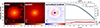 |
Fig. 4. Sersic fit in the F115W band for the example BGG at z = 0.22, shown in the top-left panel of Fig. 5. The F150W, F277W, and F444W bands are available in the attached pdf file through Zenodo in Sect. 6. |
Figure 5 shows a color composite of the central BGGs in COSMOS-Web groups spanning redshifts from z = 0.22 to z = 3.09. For the BGG in the top-left panel, we overlaid diffuse X-ray contours from Chandra and XMM-Newton archival data on the JWST RGB band made using all NIRCam bands (F115W, F150W, F277W, and F444W).
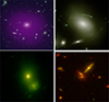 |
Fig. 5. Examples of JWST/NIRCam color composites of BGGs in COSMOS-Web groups spanning redshifts from z = 0.22 to z = 3.09. The images display diverse morphologies and structural features, including compact spheroids, disturbed or merging systems, and prominent lensing arcs in massive group cores. |
For completeness, we include in the appendix the corresponding Sérsic fits for the example BGGs presented in the top-right and lower panels of Fig. 5 (Figure C.1), (Figure C.2), and (Figure C.3). These comparisons provide a consistent view of BGG structures across the near-infrared spectrum, enabling accurate rest-frame optical size estimates for galaxies at different redshifts. The morphological integrity and fit quality observed across these bands further demonstrate the robustness of the Galight pipeline and confirm the fidelity of our structural parameter measurements.
3.2. Rest-frame optical size selection across redshift
A key objective of this work was to study the evolution of BGG sizes in the rest-frame optical regime. Because JWST/NIRCam probes different rest-frame wavelengths depending on redshift, we employed a redshift-dependent filter selection strategy to ensure consistency in rest-frame measurements. Our target rest-frame wavelength was approximately 8000 Å, which lies near the red end of the optical spectrum.
To define rest-frame optical-to-NIR size measurements, for each galaxy we selected the NIRCam filter whose observed wavelength best samples the rest-frame ∼7000–11 000 Å range at its redshift. While this does not always coincide with the canonical rest-frame optical band (4000–6000 Å), it ensures high signal-to-noise morphological measurements across a wide redshift interval, leveraging the deepest COSMOS-Web imaging available.
Rest-frame optical imaging is preferred over the UV for structural analysis because it traces older stellar populations and is less affected by clumpy star formation and patchy dust, resulting in more robust and representative size estimates. Specifically, we adopted the following filter selections:
-
F115W for 0.05 < z ≤ 0.4
-
F150W for 0.4 < z ≤ 1.0
-
F277W for 1.0 < z ≤ 3.0
-
F444W for 3.0 < z ≤ 4.0
These observed-frame filters broadly correspond to rest-frame optical and NIR wavelengths, enabling consistent structural measurements of BGGs over nearly 12 billion years of cosmic time.
After applying all quality cuts and the redshift-based filter mapping, we obtained a high-quality sample of BGGs with rest-frame optical size measurements spanning 0.08 < z < 3.7. Angular sizes were converted to physical sizes in kiloparsecs using the Planck18 cosmology Aghanim et al. 2020.
4. Results
4.1. Size–mass relation of star-forming and quiescent BGGs
We investigated the size–mass relation of BGGs over cosmic time by dividing them into SF or QG populations using the combined classification scheme (Section 2.4), which integrates both rest-frame NUV–r–J colors and redshift-dependent sSFR thresholds. This enabled a clean comparison of structural scaling relations across stellar mass and redshift, minimizing contamination from transitional systems.
To ensure robust measurements when modeling the size-mass relation, we applied a stellar mass cut of log(M*/M⊙) > 10.0 and excluded galaxies with unreliable size estimates, requiring Re > 0.5 kpc. These thresholds were motivated by the completeness of the photometric catalogs, the PSF-limited resolution of NIRCam imaging, and the desire to minimize systematic biases in the structural fits.
 |
Fig. 6. Rest-frame wavelength probed by each COSMOS-Web NIRCam filter as a function of redshift. The shaded region indicates the approximate rest-frame optical window around 8000 Å. |
The size-mass relation is modeled using a power-law form:
![Mathematical equation: $$ \begin{aligned} \log _{10}(R_e/\mathrm{kpc} ) = \log A + \alpha \left[\log _{10}(M_*/ 5 \times 10^{10} M_\odot )\right], \end{aligned} $$](/articles/aa/full_html/2025/11/aa56085-25/aa56085-25-eq8.gif) (4)
(4)
where Re is the effective (half-light) radius in kiloparsecs, and M* is the stellar mass. We normalized the relation at a pivot mass of 5 × 10¹⁰ M⊙, chosen to reduce covariance between the slope α and the intercept log A during regression.
The slope α quantifies the degree to which galaxy size scales with stellar mass, while log A characterizes the typical size at the pivot mass. Together, these parameters provide insights into the structural growth mechanisms of BGGs and their dependence on star formation state and redshift.
The best-fit values of α and log A were obtained by Bayesian Markov Chain Monte Carlo (MCMC) inference, and the shaded bands in the figures represent the 1σ posterior uncertainties from the marginalized distributions of these parameters.
Figure 7 presents the size–mass distributions in ten redshift bins from z = 0 to z = 3.7, with blue circles representing SFGs and red circles indicating QGs. Solid (brown and blue) lines show the best-fit power law relations with shaded bands marking the 1σ uncertainties from the Bayesian fits. The vertical and horizontal dashed lines represent the stellar mass cut of log(M*/M⊙) > 10.0 and the size cut of Re > 0.5 kpc.
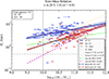 |
Fig. 7. Size–mass relation of BGGs classified using the consensus (color+sSFR) method, shown here for the redshift bin z = 0.5−1.0. Blue circles represent star-forming BGGs, and red hexagons show quiescent BGGs. Solid and dashed lines indicate best-fit power-law relations for QGs and SFGs, respectively, with shaded bands showing the 1σ uncertainties. Dash-dotted cyan and dotted orange lines show comparison relations from Faisst et al. 2017, while dashed lime and magenta lines show results from van der Wel et al. 2014. Vertical and horizontal gray lines mark the stellar mass limit of log10 (M∗/M⊙) > 10 and size cut of Re > 0.5 kpc, which are applied when fitting the relations. While BGGs follow similar evolutionary trends, they tend to be slightly smaller at fixed mass-particularly among quiescent centrals-highlighting the influence of group environments on galaxy structure. The size–mass relations for all other redshift bins are available in Section 6. |
Across the panels, we observe clear trends. At low redshift (z < 1), SFGs display systematically larger effective radii than QGs at fixed mass, with shallower slopes (α ∼ 0.1–0.2 for SFGs vs. α ∼ 0.4–0.5 for QGs), consistent with disk-dominated versus spheroid-dominated structures. Between 1 < z < 2, the SFGs continue to show relatively flat slopes, while the QGs maintain steeper size–mass relations. The difference in normalization persists, but the scatter increases. At high redshift (z > 2), the trends flatten for both populations, with larger dispersion and overlapping distributions. The small QG sample in the highest bin (z > 3.25) limits firm conclusions, but the results hint at compact, early-forming quiescent systems. We compared these trends with measurements from the literature. Dashed-dotted cyan and dotted orange lines show the relations from Faisst et al. 2017, who focused on ultra-massive galaxies (UMGs; log M*/M⊙ > 11.4) using UltraVISTA/3D-HST, while dashed lime (SFGs) and dashed magenta (QGs) lines show the relations from van der Wel et al. 2014, based on CANDELS and 3D-HST data.
Overall, the BGGs in our sample follow broadly similar evolutionary trends, but tend to exhibit slightly smaller sizes at fixed mass compared to field UMGs, especially among the quiescent population. This offset may reflect environmental effects such as earlier assembly, denser merger histories, or suppressed late-time accretion in central group environments. Importantly, while Faisst et al. 2017 focus on the most massive galaxies, our BGG sample extends across a broader mass range (log M*/M⊙ ∼ 10–12), allowing a more detailed view of the mass dependence within group central galaxies.
We also compared our results with the canonical relations from van der Wel et al. 2014, widely used as a reference for the global galaxy population. Our SFGs and QGs generally lie close to these reference tracks, although QGs in particular show a tendency toward more compact sizes at z < 2, reinforcing the idea that environmental quenching leads to more compact quiescent systems compared to field counterparts.
For completeness, we also compute size–mass relations using the individual classification methods: sSFR thresholds and (ii) NUV–r–J color cuts, which yield broadly similar slopes and intercepts, but with slightly elevated scatter, especially at intermediate redshifts (1 < z < 2) where classification uncertainties from dust and photometric noise are higher.
Taken together, these results demonstrate that BGGs follow the general size–mass evolutionary patterns seen in the broader galaxy population but show distinct signatures of environment-driven evolution, particularly among quiescent centrals.
4.2. Redshift evolution of the size–mass relation slope and intrinsic scatter
To quantify how the structural scaling of BGGs evolves over cosmic time, we traced the slope α of the size–mass relation and the intrinsic scatter σ (log Re) across ten redshift bins from z = 0.08 to z = 3.7. These parameters were derived from Bayesian fits (Eq. (4)) applied to BGGs with stellar masses log(M∗/M⊙) > 10.0. The best-fit values are listed in Table D.1 and their evolution is visualized in Fig. 8. Figure 8 presents the redshift evolution of both parameters for star-forming and quiescent BGGs, classified using three schemes: rest frame color–color selection, sSFR threshold, and their intersection. The top panel shows the evolution of the slope α (z), while the bottom panel shows σ (log Re)(z).
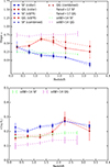 |
Fig. 8. Redshift evolution of the size–mass relation slope α (top panel) and intrinsic scatter σ (log Re) (bottom panel) for BGGs classified using color (solid lines), sSFR (dashed lines), and consensus (dotted lines) methods. Star-forming and quiescent BGGs are shown in blue and red, respectively. Quiescent BGGs display consistently steeper slopes, especially at z ∼ 1–3, while star-forming BGGs maintain nearly flat relations across redshift. The scatter increases toward higher redshift for both types, indicating greater structural diversity and formation variability in the early universe. |
4.2.1. Slope evolution.
Across all classification methods, quiescent BGGs consistently exhibit steeper size–mass slopes than their star-forming counterparts. At intermediate to high redshifts (z ∼ 1–3), quiescent systems reach slopes of αQG ∼ 0.5–0.7, suggesting stronger mass-dependent size growth, likely driven by dry mergers and inside-out structural evolution. These values are broadly consistent with earlier results from Faisst et al. 2017 and van der Wel et al. 2014. Star-forming BGGs, on the other hand, exhibit shallower and more uniform slopes (αSF ∼ 0–0.2) across all redshifts. This supports a scenario in which size growth in these systems is nearly mass independent, likely reflecting disk-dominated morphologies and gradual gas accretion. A mild decline in slope toward higher redshifts suggests a more homogeneous structural state in early epochs, before significant mass-driven morphological differentiation emerges.
4.2.2. Scatter evolution.
The intrinsic scatter σ (log Re) increases with redshift for both types of galaxy, reaching ∼ 0.3 –0.4 dex at z > 2. Star-forming BGGs generally show higher scatter than quiescent ones, especially beyond z ∼ 2, consistent with a broader diversity in morphology and assembly histories, such as clumpy star formation and disturbed stellar structures. In quiescent BGGs, the increase in scatter likely reflects varied evolutionary paths involving compaction, rapid quenching, and merger-driven size buildup. Compared to van der Wel et al. 2014, our quiescent sample shows a systematically larger scatter, potentially highlighting the role of halo mass and environment in shaping the structural diversity of BGGs. Together, the evolving slope and scatter suggest that quiescent BGGs undergo a more mass-dependent, hierarchical assembly, while star-forming systems evolve along more regulated, secular growth tracks. The increasing scatter at high redshift reflects a broader range of formation mechanisms, consistent with the transition from dynamically active early phases to more settled structural relations in the local Universe.
4.3. Size evolution of BGGs at fixed stellar mass
To investigate the redshift evolution of BGG sizes at fixed stellar mass log(M*/M⊙) = 10.7, we fit the relation
 (5)
(5)
where Re and z represent the effective radius and redshift of the galaxy, respectively, and A and α are the intercept and slope of the relation. We performed this analysis separately for star-forming and quiescent BGGs, defined using three different classification schemes: (1) rest-frame NUV-r-J color diagram, (2) sSFR, and (3) a combined color+sSFR criterion.
Figure 9 shows the best-fit size-redshift relations for each population, with shaded bands indicating the 1σ uncertainty envelopes from the model fits. Our results demonstrate that BGGs experience substantial size growth over cosmic time. Across all classification schemes, quiescent BGGs show systematically steeper evolutionary slopes (larger α) than their star-forming counterparts, indicating stronger size growth since high redshift. This suggests that while quiescent BGGs likely underwent an early compaction phase followed by significant size increase-possibly through dissipationless (dry) mergers - star-forming BGGs exhibit a more moderate size evolution, likely reflecting gradual growth through continued star formation and gas accretion.
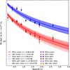 |
Fig. 9. Redshift evolution of the effective radius (Re) of star-forming (blue) and quiescent (red) BGGs at fixed stellar mass M* = 5 × 10¹⁰ M⊙. BGGs are classified using three criteria: rest-frame NUV-r-J color (solid lines), sSFR (dashed lines), and combined color+sSFR (dotted lines). Curves show the best-fit relation Re ∝ (1 + z)−α, with shaded regions indicating 1σ confidence intervals. Star-forming BGGs exhibit stronger size evolution than quiescent ones in all classification schemes. The slight offset seen at z ∼ 0.6 may reflect sample scatter or minor overfitting effects in some models. |
The best-fit slopes (α) for Re ∝ (1 + z)−α are summarized in Table 1. Table 1 also lists the growth factor of the BGG size (Re(zmin)/Re(zmax)) for both SFs and QGs.
Best-fit parameters of the size–mass relation for BGGs.
We note a slight deviation between the model and the data around z ∼ 0.6, particularly for star-forming BGGs. This may indicate overfitting due to increased scatter or sample variance in that redshift interval. Future analyses incorporating larger samples and improved error modeling will help clarify this localized discrepancy.
4.4. Size distribution of BGGs across cosmic time
To better understand the statistical nature and intrinsic scatter of the size distribution of BGGs, we examined the one-dimensional distribution of  for star-forming and quiescent BGGs within seven redshift intervals spanning
  . Figure 10 presents normalized histograms for both populations, without binning by stellar mass, ensuring that the full population-wide size distribution is represented at each epoch.
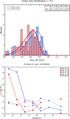 |
Fig. 10. Normalized size distributions of BGGs in log scale for the z = 0.0−0.5 bin and a summary panel tracking the evolution of the fitted parameters across all redshift bins. Star-forming galaxies (SFGs) and quiescent galaxies (QGs) are shown as blue and red histograms, respectively. Dashed lines indicate best-fit skewed normal functions, with annotated parameters-mean μ, standard deviation σ, and skewness a. At low redshift, QGs appear more compact and less scattered than SFGs, which exhibit broader, more asymmetric distributions. The full set of redshift-dependent size distributions is available in Section 6. |
In each panel, SFGs are shown in blue and QGs in red. We fit a skewed normal function to each distribution using maximum likelihood estimation, with the best-fit parameters – mean (μ), standard deviation (σ) and skewness (a) – displayed in the legend of each panel. The summary plot in the bottom-right panel tracks the evolution of μ and σ as a function of redshift.
At low redshift (z ≲ 1.5), the quiescent population exhibits a more compact and narrower distribution (μ ∼ 0.7, σ ∼ 0.25), while the star-forming BGGs tend to be larger and more broadly distributed (μ ∼ 0.8–0.9, σ ∼ 0.3–0.35). The skewness parameter a suggests that QGs typically show low or moderate asymmetry, while SFGs display stronger asymmetry or broadening toward larger sizes.
At higher redshifts (z > 2), the number of quiescent BGGs rapidly declines and their distributions become sparse, making reliable fits more challenging. In contrast, SFGs remain numerous at high redshifts and retain a broad, right-skewed size distribution, reflecting their continued structural diversity and active assembly.
This analysis shows that star-forming and quiescent BGGs occupy distinct structural regimes across cosmic time, with QGs being significantly more compact and tightly distributed, while SFGs maintain broader and more asymmetric size profiles. The width and asymmetry of these distributions provide further evidence of differing evolutionary pathways, likely shaped by differences in gas accretion, star formation activity, and merger histories.
4.5. Size distributions of BGGs across redshift and stellar mass
To further explore the structural properties of BGGs, we investigated the distribution of galaxy sizes within redshift and stellar mass bins. Figure 11 presents histograms of the effective logarithmic radius ( ) for BGGs (SFGs and QGs), classified using the combined rest-frame color–color– and redshift–dependent sSFR criteria. The distributions are shown for two stellar mass intervals (
 and
and  ), across six redshift bins from z = 0 to z = 3.7.
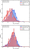 |
Fig. 11. Distributions of |


Each panel displays normalized histograms for SFGs (blue) and QGs (red), overlaid with best-fit skew-normal probability density functions. For each population and bin, we annotate the fitted skewness parameters (a), location (μ), and scale (σ). These provide a detailed statistical summary of the shape, width, and asymmetry of the distribution across cosmic time.
At low redshifts (z < 1.5), quiescent BGGs show compact and narrow size distributions, with peaks around μ ∼ 0.3–0.6, consistent across both mass bins. In contrast, star-forming BGGs show broader and more asymmetric distributions, especially in the lower mass bin, often skewed toward smaller sizes. This reflects the structural diversity and clumpy star-forming morphologies in low-mass SFGs.
In the high-mass bin, a noticeable bimodality is observed between SFGs and QGs up to z ∼ 1.5, where the separation in the median size becomes most distinct. Beyond z > 2, the quiescent population becomes sparse, particularly in the low-mass bin, reflecting delayed quenching in less massive systems. At these redshifts, SFGs dominate the sample and maintain broad, right-skewed size distributions, reflecting active disk growth and gas accretion.
Figure 12 summarizes the redshift evolution of the fitted μ (mean log10Re) and σ (scatter) parameters for each mass bin and galaxy type. For both mass bins, the SFGs show systematically higher mean sizes than the QGs at all redshifts. Both populations show a decline in μ with increasing redshift, but the decline is steeper for SFGs, particularly in the high-mass bin. The scatter σ increases modestly with redshift for both SFGs and QGs, but the increase is more noticeable for SFGs, especially at z > 2, indicating greater structural diversity in earlier epochs. In contrast, QGs maintain consistently narrower scatter across cosmic time, reflecting their more homogeneous and settled morphologies. In summary, these findings emphasize the evolution of BGG sizes based on mass and type, showing diverse, extended growth in SFGs and initial compaction with later passive size changes in QGs.
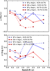 |
Fig. 12. Summary of the redshift evolution of the fitted mean (μ, top) and scatter (σ, bottom) of log10Re distributions for BGGs in two stellar mass bins ( |


For a complementary overview using two broad redshift bins to boost statistical power, see Appendix E. In addition to sizes, we examined the redshift evolution of the Sérsic index and ellipticity for quiescent BGGs, following similar approaches used in recent field and cluster studies De Propris et al. 2016; Mitsuda et al. 2017; Cerulo et al. 2017; Chan et al. 2018. Both parameters show a slight evolution toward diskier morphologies at higher redshift, with BGGs remaining rounder (Δϵ ∼ 0.02 − 0.04) and more concentrated (Δn ∼ 0.2 − 0.5) than field quiescents at fixed z. The complete results are presented in Appendix F.
5. Discussion and conclusions
We present the first comprehensive study of BGG structural evolution from z = 0.08 to z = 3.7 using COSMOS-Web NIRCam observations. Our results reveal that BGGs follow the general size evolution trends observed in field galaxies, but with systematic environmental modifications. The measured size growth slopes (α = 1.11–1.40) are consistent with previous studies of massive galaxies van der Wel et al. 2014; Faisst et al. 2017, confirming that the fundamental processes driving size evolution operate similarly across environments. However, BGGs are systematically more compact than field galaxies at fixed mass, particularly among quiescent systems. This environmental effect likely reflects several mechanisms: (1) earlier assembly in overdense regions, (2) suppressed late-time gas accretion due to environmental heating, and (3) increased merger activity within group-scale halos. The steeper size evolution of quiescent BGGs (α = 1.24) compared to star-forming systems (α = 0.96) supports a two-phase evolutionary scenario in which quiescent BGGs underwent early compaction during their active phase, followed by substantial size growth through minor mergers after quenching. This interpretation is consistent with the higher mass-dependence of their size–mass relations and their systematically compact nature. Star-forming BGGs exhibit more moderate size evolution, suggesting growth through gradual processes such as gas accretion and disk assembly. The shallower size–mass slopes and larger intrinsic scatter in this population reflect ongoing structural evolution and diversity in formation pathways. Our measurements provide crucial constraints for theoretical models of galaxy formation in group-scale environments, highlighting the importance of environmental effects in semi-analytic models and cosmological simulations. The mass-dependent size scaling we observe, particularly for quiescent systems, suggests that merger-driven growth becomes increasingly important above M* ∼ 1011 M⊙, aligning with theoretical predictions for dry merger efficiency in massive halos. Our main conclusions are as follows.
Systematic structural differences: Quiescent BGGs are more compact than star-forming counterparts across all redshifts, with steeper size–mass slopes indicating stronger mass-dependent scaling. In addition to size evolution, we find that quiescent BGGs remain rounder and more centrally concentrated than stellar-mass-matched field quiescents at all redshifts, while both populations become modestly diskier toward high z (Appendix F), consistent with earlier assembly and merger-driven growth in group centrals.
Differential size evolution: At fixed stellar mass, quiescent BGGs show steeper size evolution (α = 1.40 ± 0.09) than star-forming systems (α = 1.11 ± 0.07), suggesting different growth mechanisms.
Environmental effects: BGGs are systematically smaller than field galaxies at fixed mass, particularly quiescent systems, highlighting environmental suppression of size growth.
Increasing structural diversity: Intrinsic scatter in size relations increases toward higher redshift, reaching ∼0.3–0.4 dex at z > 2, reflecting greater formation pathway diversity in the early Universe.
Robustness across methods: The results persist across different classification schemes, confirming the physical reality of the observed trends. These findings establish BGGs as valuable probes of environment-dependent galaxy evolution and provide essential benchmarks for theoretical models. The unprecedented statistical power and redshift baseline of COSMOS-Web enable detailed characterization of structural scaling relations in group environments for the first time. Future work will explore the connection between structural properties and star formation activity in BGGs, investigating how quenching processes drive morphological transformation and the role of the active galactic nucleus (AGN) feedback in regulating galaxy growth. Combined with upcoming surveys, these studies will provide a complete picture of how environment shapes galaxy evolution across cosmic time. A complete bulge-disk decomposition would help unravel the contributions of disk star formation and bulge growth in BGGs. However, such an analysis requires a spatial resolution and S/N higher than those available for the full redshift range considered here; we therefore defer this analysis to future work with next-generation, deep, high-resolution imaging.
Data availability
Tables containing the COSMOS-Web BGG catalog are available at the CDS via https://cdsarc.cds.unistra.fr/viz-bin/cat/J/A+A/703/A129.
The brightest group galaxy (BGG) catalog is available at Zenodo. Additional analysis figures are provided as supplementary material at Zenodo.
Acknowledgments
We acknowledge the contribution of the COSMOS collaboration, consisting of more than 200 scientists. More information about the COSMOS survey can be found at https://cosmos.astro.caltech.edu/. This work was made possible by using the CANDIDE cluster at the Institut d’Astrophysique de Paris. The cluster was funded through grants from the PNCG, CNES, DIM-ACAV, the Euclid Consortium, and the Danish National Research Foundation Cosmic Dawn Center (DNRF140). It is maintained by Stephane Rouberol. Part of this work was supported by the German Deutsche Forschungsgemeinschaft, DFG project number Ts 17/2–1. Part of this research was carried out at the Jet Propulsion Laboratory, California Institute of Technology, under a contract with the National Aeronautics and Space Administration (80NM0018D0004). French COSMOS team members are partly supported by the Centre National d’Etudes Spatiales (CNES). We acknowledge the funding of the French Agence Nationale de la Recherche for the project iMAGE (grant ANR-22-CE31-0007). LM acknowledges the financial contribution from the PRIN-MUR 2022 20227RNLY3 grant “The concordance cosmological model: stress-tests with galaxy clusters" supported by Next Generation EU and from the grant ASI n. 2024-10-HH.0 “Attività scientifiche per lamissione Euclid – fase E”.
References
- Aghanim, N., Akrami, Y., Ashdown, M., et al. 2020, A&A, 641, A6 [NASA ADS] [CrossRef] [EDP Sciences] [Google Scholar]
- Arnouts, S., Moscardini, L., Vanzella, E., et al. 2002, MNRAS, 329, 355 [Google Scholar]
- Bellagamba, F., Roncarelli, M., Maturi, M., & Moscardini, L. 2018, MNRAS, 473, 5221 [NASA ADS] [CrossRef] [Google Scholar]
- Belli, S., Newman, A. B., Ellis, R. S., & Konidaris, N. P. 2014, ApJ, 788, L29 [Google Scholar]
- Belli, S., Newman, A. B., & Ellis, R. S. 2015, ApJ, 799, 206 [NASA ADS] [CrossRef] [Google Scholar]
- Bertin, E. 2011, ASP Conf. Ser., 442, 435 [Google Scholar]
- Bertin, E., Schefer, M., Apostolakos, N., et al. 2020, ASP Conf. Ser., 527, 461 [NASA ADS] [Google Scholar]
- Birrer, S., Shajib, A., Gilman, D., et al. 2021, J. Open Source Software, 6, 3283 [NASA ADS] [CrossRef] [Google Scholar]
- Bocquet, S., Dietrich, J. P., Schrabback, T., et al. 2019, ApJ, 872, 2 [Google Scholar]
- Boquien, M., Burgarella, D., Roehlly, Y., et al. 2019, A&A, 622, A103 [NASA ADS] [CrossRef] [EDP Sciences] [Google Scholar]
- Bruzual, G., & Charlot, S. 2003, MNRAS, 344, 1000 [NASA ADS] [CrossRef] [Google Scholar]
- Calzetti, D., Armus, L., Bohlin, R. C., et al. 2000, ApJ, 533, 682 [NASA ADS] [CrossRef] [Google Scholar]
- Casey, C. M., Kartaltepe, J. S., Drakos, N. E., et al. 2023, ApJ, 954, 31 [NASA ADS] [CrossRef] [Google Scholar]
- Cerulo, P., Couch, W. J., Lidman, C., et al. 2017, MNRAS, 472, 254 [NASA ADS] [CrossRef] [Google Scholar]
- Chan, J. C. C., Beifiori, A., Saglia, R. P., et al. 2018, ApJ, 856, 8 [NASA ADS] [CrossRef] [Google Scholar]
- Cui, W. 2024, ArXiv e-prints [arXiv:2406.03829] [Google Scholar]
- De Lucia, G., & Blaizot, J. 2007, MNRAS, 375, 2 [Google Scholar]
- De Propris, R., Bremer, M. N., & Phillipps, S. 2016, MNRAS, 461, 4517 [CrossRef] [Google Scholar]
- Ding, X., Silverman, J., Treu, T., et al. 2020, ApJ, 888, 37 [NASA ADS] [CrossRef] [Google Scholar]
- Faisst, A. L., Carollo, C. M., Capak, P. L., et al. 2017, ApJ, 839, 71 [NASA ADS] [CrossRef] [Google Scholar]
- Franco, M., Akins, H. B., Casey, C. M., et al. 2024, ApJ, 973, 23 [NASA ADS] [CrossRef] [Google Scholar]
- Franco, M., Casey, C. M., Koekemoer, A. M., et al. 2025, ArXiv e-prints [arXiv:2506.03256] [Google Scholar]
- George, A., Damjanov, I., Sawicki, M., et al. 2025, ApJ, 987, 45 [Google Scholar]
- Gozaliasl, G., Finoguenov, A., Khosroshahi, H. G., et al. 2016, MNRAS, 458, 2762 [NASA ADS] [CrossRef] [Google Scholar]
- Gozaliasl, G., Finoguenov, A., Khosroshahi, H. G., et al. 2018, MNRAS, 475, 2787 [CrossRef] [Google Scholar]
- Gozaliasl, G., Finoguenov, A., Tanaka, M., et al. 2019, MNRAS, 483, 3545 [Google Scholar]
- Gozaliasl, G., Finoguenov, A., Khosroshahi, H. G., et al. 2020, A&A, 635, A36 [EDP Sciences] [Google Scholar]
- Harish, S., Kartaltepe, J. S., Liu, D., et al. 2025, ArXiv e-prints [arXiv:2506.03306] [Google Scholar]
- Ilbert, O., Arnouts, S., McCracken, H. J., et al. 2006, A&A, 457, 841 [NASA ADS] [CrossRef] [EDP Sciences] [Google Scholar]
- Ilbert, O., McCracken, H. J., Le Fèvre, O., et al. 2013, A&A, 556, A55 [NASA ADS] [CrossRef] [EDP Sciences] [Google Scholar]
- Khostovan, A. A., Kartaltepe, J. S., Salvato, M., et al. 2025, ArXiv e-prints [arXiv:2503.00120] [Google Scholar]
- Koekemoer, A. M., Aussel, H., Calzetti, D., et al. 2007, ApJS, 172, 196 [Google Scholar]
- Koester, B. P., McKay, T. A., Annis, J., et al. 2007, ApJ, 660, 239 [NASA ADS] [CrossRef] [Google Scholar]
- Kravtsov, A. V., et al. 2018, MNRAS, 481, L70 [Google Scholar]
- Kriek, M., van Dokkum, P. G., Franx, M., Illingworth, G. D., & Magee, D. K. 2009, ApJ, 705, L71 [NASA ADS] [CrossRef] [Google Scholar]
- Kümmel, M., Bertin, E., Schefer, M., et al. 2020, ASP Conf. Ser., 527, 29 [Google Scholar]
- Maturi, M., Bellagamba, F., Radovich, M., et al. 2019, MNRAS, 485, 498 [Google Scholar]
- Maturi, M., Finoguenov, A., Lopes, P. A. A., et al. 2023, A&A, 678, A145 [NASA ADS] [CrossRef] [EDP Sciences] [Google Scholar]
- Mitsuda, K., Doi, M., Morokuma, T., et al. 2017, ApJ, 834, 109 [NASA ADS] [CrossRef] [Google Scholar]
- Mo, H. J., Mao, S., & White, S. D. M. 1998, MNRAS, 295, 319 [Google Scholar]
- Mosleh, M., Williams, R. J., Franx, M., et al. 2012, ApJ, 756, L12 [NASA ADS] [CrossRef] [Google Scholar]
- Oesch, P. A., Bouwens, R. J., Carollo, C. M., et al. 2010, ApJ, 709, L21 [NASA ADS] [CrossRef] [Google Scholar]
- Oke, J. B. 1974, ApJS, 27, 21 [Google Scholar]
- Pacifici, C., Kassin, S. A., Weiner, B. J., et al. 2016, ApJ, 832, 79 [Google Scholar]
- Peng, C. Y., Ho, L. C., Impey, C. D., & Rix, H.-W. 2010, AJ, 139, 2097 [Google Scholar]
- Pillepich, A., et al. 2021, MNRAS, 500, 120 [Google Scholar]
- Poggianti, B. M., Moretti, A., Calvi, R., et al. 2013, ApJ, 777, 125 [NASA ADS] [CrossRef] [Google Scholar]
- Ponman, T. J., Allan, D. J., Jones, L. R., et al. 1994, Nature, 369, 462 [Google Scholar]
- Pozzetti, L., Bolzonella, M., Zucca, E., et al. 2010, A&A, 523, A13 [NASA ADS] [CrossRef] [EDP Sciences] [Google Scholar]
- Salim, S., Boquien, M., & Lee, J. C. 2018, ApJ, 859, 11 [Google Scholar]
- Scoville, N., Aussel, H., Brusa, M., et al. 2007, ApJS, 172, 1 [Google Scholar]
- Sersic, J. L. 1968, Atlas de Galaxias Australes [Google Scholar]
- Shuntov, M., Ilbert, O., Toft, S., et al. 2024, A&A, 695, A20 [Google Scholar]
- Shuntov, M., Akins, H. B., Paquereau, L., et al. 2025, ArXiv e-prints [arXiv:2506.03243] [Google Scholar]
- Stott, J. P., Collins, C. A., Burke, C., Hamilton-Morris, V., & Smith, G. P. 2011, MNRAS, 414, 445 [Google Scholar]
- Toft, S., van Dokkum, P., Franx, M., et al. 2007, ApJ, 671, 285 [CrossRef] [Google Scholar]
- Toni, G., Gozaliasl, G., Maturi, M., et al. 2025, A&A, 697, A197 [NASA ADS] [CrossRef] [EDP Sciences] [Google Scholar]
- van der Burg, R. F. J., Muzzin, A., Hoekstra, H., et al. 2014, A&A, 561, A79 [NASA ADS] [CrossRef] [EDP Sciences] [Google Scholar]
- van der Wel, A., Franx, M., van Dokkum, P. G., et al. 2014, ApJ, 788, 28 [Google Scholar]
- Williams, R. J., Quadri, R. F., Franx, M., et al. 2010, ApJ, 713, 738 [NASA ADS] [CrossRef] [Google Scholar]
- Yang, L., Silverman, J., Oguri, M., et al. 2024, MNRAS, 531, 4006 [Google Scholar]
- Yang, L., Kartaltepe, J. S., Franco, M., et al. 2025, ArXiv e-prints [arXiv:2504.07185] [Google Scholar]
Appendix A: Detailed brightest group galaxies selection methodology
A.1. Traditional BGG selection methods
Traditionally, BCGs and BGGs have been identified through either luminosity-based selection (choosing the most luminous galaxy in a given band, typically r-band) or stellar mass-based selection (selecting the most massive galaxy in the system) De Lucia & Blaizot 2007; Koester et al. 2007; Gozaliasl et al. 2019. In particular, in the definition of fossil groups, the magnitude of the r band determines the gap between the magnitudes of the two brightest membersPonman et al. 1994.
A.2. Hybrid selection algorithm
We identified BGGs in the COSMOS-Web galaxy group catalog Toni et al. 2025 using a hybrid selection method that combines stellar mass and luminosity criteria. Building on Gozaliasl et al. 2019, 2020, we address two key limitations of traditional approaches: (1) the spatial offset of BGGs from group centers in low-mass systems, and (2) the contamination by starburst galaxies in luminosity-based selections.
Our methodology processes galaxies within fixed apertures of 250 kpc and 500 kpc (also tested at 750 kpc) from the group centers, implementing a two-stage selection algorithm. First, we filter the galaxy sample by applying a redshift constraint, which requires Δz < 0.05(1 + z) relative to the group candidate, to ensure that the selection remains confined to the vicinity of the group in redshift space. Among this filtered sample, we identify the luminosity-selected BGG as the galaxy with the lowest apparent magnitude m in the F150W band, unless the magnitude difference between the first and second brightest galaxies is less than 0.5 mag; in that case, we choose the one with the highest membership probability.
In parallel, we repeat the selection using the median stellar mass derived from LePhare instead of magnitude. Here, we select the most massive galaxy as the mass-selected BGG, unless the logarithmic mass difference between the most massive and the second most massive galaxy is smaller than 0.25 dex; in that case, we again select the one with the higher membership probability. For all detections, we store both the first and second candidates according to these criteria. This approach ensures that each group has both a mass-selected and a luminosity-selected BGG, providing a robust cross-check of group-centric galaxy identification.
For each group, we evaluated two primary candidates: the galaxy with the highest median stellar mass and the brightest galaxy. We then compare the stellar mass and r-band luminosity of both candidates for a given group. The selection incorporates aperture-dependent corrections, preferentially choosing 250 kpc candidates when: (a) for mass-selected BGGs, the mass difference is ≤ 0.1 dex; and (b) for luminosity-selected BGGs, the magnitude difference is ≤ 0.15 mag relative to 500 kpc candidates.
The final hybrid selection applies a tiered decision tree:
-
Selects the mass-dominant galaxy if its stellar mass exceeds the luminosity-selected candidate by ≥ 0.1 dex
-
Chooses the luminosity-dominant galaxy if it is brighter by an equivalent mass margin
-
Defaults to the brighter galaxy when mass differences are < 0.1 dex, weighting recent star formation
A.3. Selection results and validation
Validation includes cross-matching with a master galaxy catalog to eliminate spurious detections, producing three output catalogs: pure mass-selected, pure luminosity-selected, and hybrid-selected BGGs. A total of 1,294 BGGs were selected on the basis of stellar mass, ensuring the identification of the most massive galaxies within each group. Additionally, 384 BGGs were selected using a luminosity-based criterion, which identifies the brightest galaxies. For a more comprehensive selection that accounts for both mass and luminosity, we included 803 BGGs selected within a 250 kpc radius from the group center, and 875 BGGs selected within a 500 kpc radius. This combined approach ensures a more accurate representation of the BGG population, minimizing selection biases and capturing galaxies with both high stellar mass and luminosity.
As shown in Fig. A.1, a luminosity-based selection at the low stellar mass end misses some true BGGs, whereas our hybrid method ensures a more complete sample by balancing both criteria. The accompanying histograms demonstrate how smaller apertures (250 kpc) bias selections toward lower luminosity and mass values, frequently misidentifying satellites as BGGs. By combining mass and luminosity metrics across multiple apertures, we significantly reduce selection biases and more accurately represent the true BGG population across diverse group environments, from compact to loosely bound systems.
Each galaxy group in the catalog is detected using the AMICO algorithm, and galaxies are assigned membership probabilities based on their photometric redshifts and spatial distribution. We consider galaxies with a group membership probability, ensuring a high-confidence sample of true group members. For further information on determining the group membership and assigning a membership probability for each group galaxy we refer the reader to Toni et al. 2025.
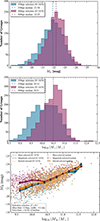 |
Fig. A.1. Selection and characterization of BGGs in the COSMOS-Web galaxy group catalog. The top and middle panels show histograms of the number of groups as a function of log stellar mass (log10(M*/M⊙) and absolute magnitude (MR), comparing selections based on two different aperture sizes: 250 kpc (blue) and 500 kpc (magenta). The bottom panel displays a scatter plot of absolute magnitude (MR) versus log stellar mass (log10(M*/M⊙), with points color-coded by selection method: mass-selected (blue circles), magnitude-selected (red squares), and hybrid-selected (green triangles). The solid brown, blue dash-dotted, and magenta dashed lines represent the medians for mass-selected, magnitude-selected, and hybrid-selected methods. The shaded regions around the median lines show the corresponding confidence bands. |
A.4. Selection method comparison
To assess the consistency and robustness of BGG identification methods, we compared stellar mass- and luminosity-based selection across our sample of galaxy groups. The two methods agreed on the BGG in 48.7% of the systems. For the remaining groups, the stellar mass difference between the selected BGGs, Δlog10(M⋆), has a median of 0 and a standard deviation of 0.46 dex, with 65. 7% of the groups exhibiting differences less than 0.3 dex, and 5.7% showing catastrophic disagreement (Δlog10(M⋆) > 1 dex). The difference in absolute magnitude of the R band, ΔMR, shows a wider spread with a standard deviation of 0.62 mag.
To mitigate inconsistencies between these two approaches, we implemented the hybrid BGG selection strategy that combines stellar mass and luminosity ranking. The hybrid selected BGG matched the mass-based BGG in 77.1% of the groups and the mag-based BGG in 71.6%, demonstrating improved overlap with both selection criteria. These findings confirm that,, while mass and luminosity selections individually perform well in many cases, a hybrid method offers a more robust and consistent approach to BGG identification across a diverse range of environments.
A summary of these comparisons is shown in Figure A.2, which includes violin plots of the stellar mass distributions for each selection method (left), cumulative distribution functions (CDFs) of absolute differences in stellar mass and R-band magnitude between mass- and mag-selected BGGs (center), and a bar chart quantifying the agreement rates between the different selection methods (right). The steep rise in the CDF at Δ = 0 reflects the significant number of exact matches, while the bar chart highlights the strong alignment of the hybrid method with both individual strategies.
To further ensure the robustness of our group and the selection of BGG, we restricted our analysis to groups rich in biodiversity λstar > 4 (see also Fig. 1 ), corresponding to groups with enough mass members to minimize contamination and projection effects. We also apply a stellar mass threshold of log(M*/M⊙) > 9 to ensure completeness across the redshift range.
A.5. BGG catalog
We construct the BGG catalog by identifying the most massive and luminous galaxy within each group in the COSMOS-Web group sample as discussed in Sec. A. Each group is characterized by its central coordinates (RA_GR, DEC_GR), redshift (Z_GR) from Toni et al. 2025, and an associated group radius defined as the hybrid radius derived from the AMICO detection algorithm. The galaxy membership within each group is determined using proximity in both spatial and redshift dimensions.
 |
Fig. A.2. Comparison of BGG selection methods. Left: Violin plots of stellar mass distributions for BGGs selected using mass-based, luminosity-based, and hybrid criteria. Center: Cumulative distribution functions (CDFs) of the absolute differences in stellar mass (Δlog10(M⋆)) and R-band magnitude (ΔMR) between mass- and mag-selected BGGs, showing that ∼65.7% of the sample has Δlog10(M⋆) < 0.3 dex, while ∼5.7% exceeds 1 dex. Right: Agreement rates between selection methods. The hybrid BGG matches the mass-based and mag-based selections in 77.1% and 71.6% of groups, respectively, while the mass and mag selections agree in only 48.7% of cases. |
The full physical properties of BGGs can be obtained from the COSMOS2025 multiwavelength catalog Shuntov et al. 2025 through cross-matching with the SE++ catalog. We use the unique galaxy identifier ID_COSMOS2025_SE++ for matching.
The BGG catalog includes the following columns:
-
Group_ID: Unique identifier of the galaxy group.
-
RA_GR, DEC_GR: Right ascension and declination of the center of the group (in degrees).
-
Z_GR: Redshift of the group.
-
Hybrid_radius: Estimated physical radius of the group in arcminutes.
-
ID_COSMOS2025_SE++: BGG source identifier from the COSMOS2025 SE++ catalog.
-
RA_DETEC, DEC_DETEC: Right ascension and declination of the detected BGG (in degrees).
-
logM: Stellar mass of the BGG, in units of log10(M⊙).
-
MR: Absolute magnitude of the rest frame in the R-band.
-
flag_type: A quality or classification flag indicating the BGG selection type or ambiguity in group membership.
This catalog serves as the basis for our subsequent structural and star-forming analyses of BGGs across cosmic time.
Appendix B: BGGs classification as star forming or quiescent
Table B.1 presents the number of BGGs classified as star-forming (SF) or quiescent (QG) using three approaches: sSFR threshold alone, rest-frame NUV–r–J color criteria alone, and the combined consensus method requiring agreement between both criteria. The consensus classification (color+sSFR) provides the most conservative sample by excluding galaxies that satisfy only one criterion, effectively filtering out transitional or ambiguous systems. Star-forming BGGs dominate at high redshift while quiescent systems become more prevalent toward lower redshifts, reflecting the cosmic evolution of galaxy populations in group environments.
Number of BGGs classified as star-forming or quiescent using color, sSFR, and combined criteria presented in Sec. 2.4 across redshift bins.
Appendix C: Multi-band sérsic fits for BGGs
To complement the structural modeling presented in the main text, we show in this appendix the Sérsic profile fits for the same three other BGGs across four JWST/NIRCam filters: F115W, F150W, F277W, and F444W. These figures provide visual confirmation of the fitting quality and structural consistency across different wavelengths.
Figures C.1-C.3 follow the same format as Figure 4 and include, for each galaxy: the original data cutout, the best-fit Sérsic model, the normalized residual map, and the azimuthally averaged radial profile comparison between data and model. Residuals remain small and symmetric in most cases, indicating robust fits. The light profiles remain stable across filters, although subtle differences in morphology and concentration are apparent due to wavelength-dependent features such as dust attenuation or star-forming clumps.
These multi-band fits allow us to trace rest-frame optical sizes over a wide redshift range and ensure that our structural parameters are not biased by single-band anomalies. Combined, these figures demonstrate the reliability and consistency of the structural measurements used in our analysis.
 |
Fig. C.1. Sersic fits for the BGG showin in lower right panel of Fig. 5 at z = 0.71 across the four JWST band. |
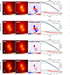 |
Fig. C.2. Sersic fits for the BGG showin in lower left panel of Fig. 5 at z= 0.81 across the four JWST band. |
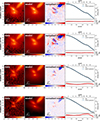 |
Fig. C.3. Sersic fits for the BGG showin in top right panel of Fig. 5 at z = 3.09 across the four JWST band. |
Appendix D: Impact of classification on size-mass relations and best fit parameters
To examine the influence of galaxy classification method, Figures D.2 and D.3 show the size-mass relations using only color-color and sSFR-based classifications, respectively. In both, we plot Re versus stellar mass in ten redshift bins up to z = 3.7, with best-fit relations for star-forming (blue) and quiescent (red) BGGs.
The results broadly agree with those in the main text based on the hybrid classification, but show modest differences in slope and scatter. This highlights the consistency of our findings and the benefit of using a consensus scheme for cleaner separation of galaxy populations. Table D.1 provides the complete set of best-fit parameters for the size–mass relation log10(Re/kpc) = log A + α[log10(M*/5 × 1010 M⊙)] derived from Bayesian MCMC fitting in each redshift bin. Parameters are shown for all three classification methods to demonstrate the robustness of our results. Quiescent BGGs consistently exhibit steeper slopes (α) and lower intercepts compared to star-forming systems across all methods and redshift bins, while intrinsic scatter generally increases toward higher redshift for both populations.
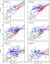 |
Fig. D.1. Size–mass relation of BGGs classified using the consensus (color+sSFR) method, shown across six redshift bins from z = 0.08 to z = 3.7. Blue circles represent star-forming BGGs, and red hexagons show quiescent BGGs. The dashed and solid lines indicate best-fit power-law relations for SFGs and QGs, respectively, with shaded bands showing 1σ uncertainties. Cyan dashed-dotted and orange dotted lines show comparison relations from Faisst et al. 2017, while dashed lime and dashed magenta lines show van der Wel et al. 2014 results. Gray vertical and horizontal lines represent the stellar mass limit of log10(M*/M⊙) > 10 and size cut of Re > 0.5 kpc, applied when fitting size-mass relation. The BGGs generally follow similar evolutionary trends but are slightly smaller at fixed mass, especially among quiescent centrals, highlighting the impact of group environment on galaxy structure. |
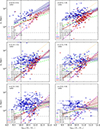 |
Fig. D.2. Size–mass relation of BGGs using color-only classification. Panels show BGGs across six redshift bins from z = 0 to z = 3.7 (Δz = 0.5). Blue circles represent star-forming BGGs and red circles show quiescent BGGs, as identified using rest-frame NUV–r–J colors. The dashed and solid lines represent best-fit size–mass relations for SFGs and QGs, respectively, with shaded regions indicating 1σ uncertainties. SFGs show generally shallower slopes and larger sizes, while QGs are more compact, especially below z ∼ 2. This classification is sensitive to dust reddening and intermediate colors. Results from Faisst et al. 2017 are shown as cyan dashed-dotted (SFGs) and orange dotted (QGs) lines in matching redshift bins for comparison. While dashed lime and dashed magenta lines show van der Wel et al. 2014 results. |
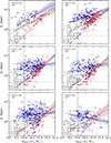 |
Fig. D.3. Size–mass relation of BGGs using sSFR-only classification. Each panel shows results for a redshift bin of width Δz = 0.5 spanning z = 0 to z = 3.7. Star-forming and quiescent BGGs are identified based on whether their log10(sSFR) falls above or below the redshift-dependent threshold log10(0.2/tobs), where tobs is the age of the universe in Gyr. As in previous figures, dashed (SFGs) and solid (QGs) lines show best-fit power-law relations, and shaded regions represent 1σ confidence intervals. The sSFR-based method yields similar trends but may misclassify dusty SFGs at intermediate redshift. Results from Faisst et al. 2017 are shown as cyan dashed-dotted (SFGs) and orange dotted (QGs) lines in matching redshift bins for comparison. While dashed lime and dashed magenta lines show van der Wel et al. 2014 results. |
Best-fit parameters of the size–mass relation for BGGs classified using color–color, sSFR, and combined (color+sSFR) criteria.
Appendix E: Size distributions in two redshift bins
To complement the detailed redshift-binned analysis presented in Section 4.5, we investigate the overall size distributions of BGGs using a simplified two-bin redshift division:  (low redshift) and
  (high redshift). This approach allows us to boost the statistical power, particularly for QGs at high redshift, and to highlight the broad contrast between early and late cosmic epochs.
Figure E.1 shows the distributions of  for BGGs split into two stellar mass bins (
 and
and  ). SFGs and QGs are shown in blue and red, respectively, with skew-normal fits overlaid. The legend in each panel reports the number of galaxies (N) and best-fit parameters for the skewness a, mean μ, and standard deviation σ.
At low redshift, both SFGs and QGs display relatively symmetric size distributions, with QGs typically more compact (lower μ) and narrower (lower σ) than their star-forming counterparts. In contrast, the high-redshift bin reveals notable asymmetry and scatter, particularly among SFGs in the low-mass bin, where the size distribution is strongly negatively skewed (a ∼ −2.9). QGs at high redshift remain small and relatively homogeneous, though their numbers are sparse, especially in the low-mass regime.
Overall, this two-bin analysis reinforces the results from the six-bin main analysis: BGG structural diversity increases at early epochs, with SFGs driving the broad and asymmetric size distributions, while QGs maintain compact, narrow profiles shaped by early quenching and passive evolution.
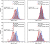 |
Fig. E.1. Distributions of log10(Re/kpc) for Brightest Group Galaxies (BGGs) in two stellar-mass bins (9.25 ≤ log10(M*/M⊙) < 10.75 and 10.75 ≤ log10(M*/M⊙) < 12.25), split into two redshift intervals (0 < z ≤ 1.5 and 1.5 < z ≤ 3.7). Star-forming galaxies (SFGs) and quiescent galaxies (QGs) are shown as blue and red histograms, respectively, with skew-normal fits overlaid (dashed for SFGs, solid for QGs). Legends list the number of galaxies and best-fit parameters a, μ, and σ. |
Appendix F: Sérsic index and ellipticity evolution of quiescent BGGs
We present the redshift evolution of the quiescent fraction, Sérsic index (n), and ellipticity (ϵ = 1 − b/a) for BGGs compared to a stellar-mass-matched field sample. The analysis follows the combined NUV–r–J + sSFR classification described in Section 2.4, ensuring a clean separation between star-forming and quiescent systems.
The Sérsic indices and ellipticities are taken from the same single-component GALIGHT fits used for the size measurements (Section 3.1), with the same PSF modeling and quality cuts applied. For each redshift bin, we compute the median value and the 16th–84th percentile range for QGs only.
Figure F.1 summarizes the results. The quiescent fraction of BGGs and field galaxies for the mass-complete subsample (M⋆ ≥ 1010 M⊙) (bottom panel) declines strongly with redshift for both BGGs and field galaxies, with BGGs remaining more quiescent by ≈5–8 percentage points at fixed redshift. The trends are consistent with those found for the full sample, confirming that our conclusions are robust to stellar mass incompleteness. For QGs, the ellipticity (middle panel) shows a mild increase toward high z, consistent with diskier morphologies in the early universe, while the Sérsic index (top panel) decreases correspondingly De Propris et al. 2016; Mitsuda et al. 2017; Cerulo et al. 2017; Chan et al. 2018; George et al. 2025. At fixed redshift, quiescent BGGs are systematically rounder (Δϵ ≈ 0.02–0.04) and more concentrated (Δn ≈ 0.2–0.5) than their field counterparts.
These trends are consistent with the interpretation that group central galaxies undergo earlier assembly and merger-driven structural evolution, leading to more spheroidal and concentrated morphologies compared to similar-mass QGs in the field.
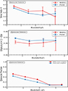 |
Fig. F.1. Redshift evolution of the median Sérsic index (n, top), median ellipticity (ϵ = 1 − b/a, middle), and quiescent fraction (bottom) for Brightest Group Galaxies (BGGs, red circles) and a stellar-mass-matched field sample (blue squares), based on the combined NUV–r–J plus sSFR classification (Sect. 2.4). Error bars represent the 16th–84th percentile range (n and ϵ) or binomial uncertainties (quiescent fraction). |
All Tables
Number of BGGs classified as star-forming or quiescent using color, sSFR, and combined criteria presented in Sec. 2.4 across redshift bins.
Best-fit parameters of the size–mass relation for BGGs classified using color–color, sSFR, and combined (color+sSFR) criteria.
All Figures
|
Fig. 1. Intrinsic richness, λ*, of detected groups and its trend with redshift. Bright group galaxies (BGGs), classified as quiescent or star-forming based on color-color criteria, are shown with red and blue points, respectively. The dashed horizontal orange line indicates the λ* limit applied in this study. |
| In the text | |
|
Fig. 2. Redshift-dependent sSFR threshold used to classify BGGs as quiescent, defined as log10(sSFR) < log10(0.2/tobs). The bottom x axis shows cosmic time in Gyr, while the top x axis shows the corresponding redshift. The threshold decreases smoothly from early to late cosmic epochs, tracing the decline in global star formation efficiency. |
| In the text | |
|
Fig. 3. Rest-frame NUV–r versus r–J color–color diagram for all BGGs combined across the full redshift range z = 0 to z = 4. Points are color-coded by their log10(sSFR/yr−1). Magenta lines delineate the quiescent region defined by |
| In the text | |
|
Fig. 4. Sersic fit in the F115W band for the example BGG at z = 0.22, shown in the top-left panel of Fig. 5. The F150W, F277W, and F444W bands are available in the attached pdf file through Zenodo in Sect. 6. |
| In the text | |
|
Fig. 5. Examples of JWST/NIRCam color composites of BGGs in COSMOS-Web groups spanning redshifts from z = 0.22 to z = 3.09. The images display diverse morphologies and structural features, including compact spheroids, disturbed or merging systems, and prominent lensing arcs in massive group cores. |
| In the text | |
|
Fig. 6. Rest-frame wavelength probed by each COSMOS-Web NIRCam filter as a function of redshift. The shaded region indicates the approximate rest-frame optical window around 8000 Å. |
| In the text | |
|
Fig. 7. Size–mass relation of BGGs classified using the consensus (color+sSFR) method, shown here for the redshift bin z = 0.5−1.0. Blue circles represent star-forming BGGs, and red hexagons show quiescent BGGs. Solid and dashed lines indicate best-fit power-law relations for QGs and SFGs, respectively, with shaded bands showing the 1σ uncertainties. Dash-dotted cyan and dotted orange lines show comparison relations from Faisst et al. 2017, while dashed lime and magenta lines show results from van der Wel et al. 2014. Vertical and horizontal gray lines mark the stellar mass limit of log10 (M∗/M⊙) > 10 and size cut of Re > 0.5 kpc, which are applied when fitting the relations. While BGGs follow similar evolutionary trends, they tend to be slightly smaller at fixed mass-particularly among quiescent centrals-highlighting the influence of group environments on galaxy structure. The size–mass relations for all other redshift bins are available in Section 6. |
| In the text | |
|
Fig. 8. Redshift evolution of the size–mass relation slope α (top panel) and intrinsic scatter σ (log Re) (bottom panel) for BGGs classified using color (solid lines), sSFR (dashed lines), and consensus (dotted lines) methods. Star-forming and quiescent BGGs are shown in blue and red, respectively. Quiescent BGGs display consistently steeper slopes, especially at z ∼ 1–3, while star-forming BGGs maintain nearly flat relations across redshift. The scatter increases toward higher redshift for both types, indicating greater structural diversity and formation variability in the early universe. |
| In the text | |
|
Fig. 9. Redshift evolution of the effective radius (Re) of star-forming (blue) and quiescent (red) BGGs at fixed stellar mass M* = 5 × 10¹⁰ M⊙. BGGs are classified using three criteria: rest-frame NUV-r-J color (solid lines), sSFR (dashed lines), and combined color+sSFR (dotted lines). Curves show the best-fit relation Re ∝ (1 + z)−α, with shaded regions indicating 1σ confidence intervals. Star-forming BGGs exhibit stronger size evolution than quiescent ones in all classification schemes. The slight offset seen at z ∼ 0.6 may reflect sample scatter or minor overfitting effects in some models. |
| In the text | |
|
Fig. 10. Normalized size distributions of BGGs in log scale for the z = 0.0−0.5 bin and a summary panel tracking the evolution of the fitted parameters across all redshift bins. Star-forming galaxies (SFGs) and quiescent galaxies (QGs) are shown as blue and red histograms, respectively. Dashed lines indicate best-fit skewed normal functions, with annotated parameters-mean μ, standard deviation σ, and skewness a. At low redshift, QGs appear more compact and less scattered than SFGs, which exhibit broader, more asymmetric distributions. The full set of redshift-dependent size distributions is available in Section 6. |
| In the text | |
|
Fig. 11. Distributions of |
| In the text | |
|
Fig. 12. Summary of the redshift evolution of the fitted mean (μ, top) and scatter (σ, bottom) of log10Re distributions for BGGs in two stellar mass bins ( |
| In the text | |
|
Fig. A.1. Selection and characterization of BGGs in the COSMOS-Web galaxy group catalog. The top and middle panels show histograms of the number of groups as a function of log stellar mass (log10(M*/M⊙) and absolute magnitude (MR), comparing selections based on two different aperture sizes: 250 kpc (blue) and 500 kpc (magenta). The bottom panel displays a scatter plot of absolute magnitude (MR) versus log stellar mass (log10(M*/M⊙), with points color-coded by selection method: mass-selected (blue circles), magnitude-selected (red squares), and hybrid-selected (green triangles). The solid brown, blue dash-dotted, and magenta dashed lines represent the medians for mass-selected, magnitude-selected, and hybrid-selected methods. The shaded regions around the median lines show the corresponding confidence bands. |
| In the text | |
|
Fig. A.2. Comparison of BGG selection methods. Left: Violin plots of stellar mass distributions for BGGs selected using mass-based, luminosity-based, and hybrid criteria. Center: Cumulative distribution functions (CDFs) of the absolute differences in stellar mass (Δlog10(M⋆)) and R-band magnitude (ΔMR) between mass- and mag-selected BGGs, showing that ∼65.7% of the sample has Δlog10(M⋆) < 0.3 dex, while ∼5.7% exceeds 1 dex. Right: Agreement rates between selection methods. The hybrid BGG matches the mass-based and mag-based selections in 77.1% and 71.6% of groups, respectively, while the mass and mag selections agree in only 48.7% of cases. |
| In the text | |
|
Fig. C.1. Sersic fits for the BGG showin in lower right panel of Fig. 5 at z = 0.71 across the four JWST band. |
| In the text | |
|
Fig. C.2. Sersic fits for the BGG showin in lower left panel of Fig. 5 at z= 0.81 across the four JWST band. |
| In the text | |
|
Fig. C.3. Sersic fits for the BGG showin in top right panel of Fig. 5 at z = 3.09 across the four JWST band. |
| In the text | |
|
Fig. D.1. Size–mass relation of BGGs classified using the consensus (color+sSFR) method, shown across six redshift bins from z = 0.08 to z = 3.7. Blue circles represent star-forming BGGs, and red hexagons show quiescent BGGs. The dashed and solid lines indicate best-fit power-law relations for SFGs and QGs, respectively, with shaded bands showing 1σ uncertainties. Cyan dashed-dotted and orange dotted lines show comparison relations from Faisst et al. 2017, while dashed lime and dashed magenta lines show van der Wel et al. 2014 results. Gray vertical and horizontal lines represent the stellar mass limit of log10(M*/M⊙) > 10 and size cut of Re > 0.5 kpc, applied when fitting size-mass relation. The BGGs generally follow similar evolutionary trends but are slightly smaller at fixed mass, especially among quiescent centrals, highlighting the impact of group environment on galaxy structure. |
| In the text | |
|
Fig. D.2. Size–mass relation of BGGs using color-only classification. Panels show BGGs across six redshift bins from z = 0 to z = 3.7 (Δz = 0.5). Blue circles represent star-forming BGGs and red circles show quiescent BGGs, as identified using rest-frame NUV–r–J colors. The dashed and solid lines represent best-fit size–mass relations for SFGs and QGs, respectively, with shaded regions indicating 1σ uncertainties. SFGs show generally shallower slopes and larger sizes, while QGs are more compact, especially below z ∼ 2. This classification is sensitive to dust reddening and intermediate colors. Results from Faisst et al. 2017 are shown as cyan dashed-dotted (SFGs) and orange dotted (QGs) lines in matching redshift bins for comparison. While dashed lime and dashed magenta lines show van der Wel et al. 2014 results. |
| In the text | |
|
Fig. D.3. Size–mass relation of BGGs using sSFR-only classification. Each panel shows results for a redshift bin of width Δz = 0.5 spanning z = 0 to z = 3.7. Star-forming and quiescent BGGs are identified based on whether their log10(sSFR) falls above or below the redshift-dependent threshold log10(0.2/tobs), where tobs is the age of the universe in Gyr. As in previous figures, dashed (SFGs) and solid (QGs) lines show best-fit power-law relations, and shaded regions represent 1σ confidence intervals. The sSFR-based method yields similar trends but may misclassify dusty SFGs at intermediate redshift. Results from Faisst et al. 2017 are shown as cyan dashed-dotted (SFGs) and orange dotted (QGs) lines in matching redshift bins for comparison. While dashed lime and dashed magenta lines show van der Wel et al. 2014 results. |
| In the text | |
|
Fig. E.1. Distributions of log10(Re/kpc) for Brightest Group Galaxies (BGGs) in two stellar-mass bins (9.25 ≤ log10(M*/M⊙) < 10.75 and 10.75 ≤ log10(M*/M⊙) < 12.25), split into two redshift intervals (0 < z ≤ 1.5 and 1.5 < z ≤ 3.7). Star-forming galaxies (SFGs) and quiescent galaxies (QGs) are shown as blue and red histograms, respectively, with skew-normal fits overlaid (dashed for SFGs, solid for QGs). Legends list the number of galaxies and best-fit parameters a, μ, and σ. |
| In the text | |
|
Fig. F.1. Redshift evolution of the median Sérsic index (n, top), median ellipticity (ϵ = 1 − b/a, middle), and quiescent fraction (bottom) for Brightest Group Galaxies (BGGs, red circles) and a stellar-mass-matched field sample (blue squares), based on the combined NUV–r–J plus sSFR classification (Sect. 2.4). Error bars represent the 16th–84th percentile range (n and ϵ) or binomial uncertainties (quiescent fraction). |
| In the text | |
Current usage metrics show cumulative count of Article Views (full-text article views including HTML views, PDF and ePub downloads, according to the available data) and Abstracts Views on Vision4Press platform.
Data correspond to usage on the plateform after 2015. The current usage metrics is available 48-96 hours after online publication and is updated daily on week days.
Initial download of the metrics may take a while.