| Issue |
A&A
Volume 704, December 2025
|
|
|---|---|---|
| Article Number | A277 | |
| Number of page(s) | 18 | |
| Section | Cosmology (including clusters of galaxies) | |
| DOI | https://doi.org/10.1051/0004-6361/202453253 | |
| Published online | 16 December 2025 | |
The perils of stacking optically selected groups in eROSITA data
The Magneticum perspective
1
European Southern Observatory, Karl Schwarzschildstrasse 2, 85748 Garching bei München, Germany
2
Excellence Cluster ORIGINS, Boltzmannstr. 2, D-85748 Garching bei München, Germany
3
Universitäts-Sternwarte, Fakultät für Physik, Ludwig-Maximilians-Universität München, Scheinerstr.1, 81679 München Germany
4
Max-Planck-Institut für Astrophysik, Karl-Schwarzschildstr. 1, 85741, Garching bei München, Germany
5
Leibniz-Institut für Astrophysik Potsdam (AIP), An der Sternwarte 16, 14482 Potsdam, Germany
6
Universität Innsbruck, Institut für Astro- und Teilchenphysik, Technikerstr. 25/8, 6020 Innsbruck, Austria
7
INAF – Osservatorio Astronomico di Trieste, Via Tiepolo 11, 34143 Trieste, Italy
8
International Centre for Radio Astronomy Research, University of Western Australia, M468, 35 Stirling Highway, Perth, WA 6009, Australia
9
McMaster University, 1280 Main Street West, Hamilton, Ontario L8S 4L8, Canada
10
Tartu University, Ülikooli 18, 50090 Tartu, Estonia
11
Shanghai Astronomical Observatory (SHAO) at the Chinese Academy of Sciences, 80 Nandan Road, Xuhui District, Shanghai 200030, China
12
IFPU – Institute for Fundamental Physics of the Universe, Via Beirut 2, I-34014 Trieste, Italy
13
INAF, Istituto di Astrofisica Spaziale e Fisica Cosmica di Milano, Via A. Corti 12, 20133 Milano, Italy
14
Center for Astrophysics | Harvard & Smithsonian, 60 Garden Street, Cambridge, MA 02138, USA
15
INAF – Osservatorio Astronomico di Bologna, Via Gobetti 93/3, 40129 Bologna, Italy
16
Max-Planck-Institut für Extraterrestrische Physik (MPE), Giessenbachstr. 1, D-85748 Garching bei München, Germany
★ Corresponding author: This email address is being protected from spambots. You need JavaScript enabled to view it.
Received:
2
December
2024
Accepted:
23
July
2025
Abstract
Context. Hydrodynamical simulation predictions are often compared with observational data without fully accounting for systematics and biases specific to observational techniques. In this study, we used the magnetohydrodynamical simulation Magneticum to create a mock dataset that replicates the observational data available for analyzing hot gas properties in extensive galaxy group samples.
Aims. Specifically, we simulated eROSITA eRASS:4 data along with a GAMA-like galaxy spectroscopic survey from the same lightcone and generated mock, optically selected galaxy catalogs using widely employed group-finding algorithms. We then applied an observational stacking technique to the mock eRASS:4 observations, and used the mock group catalogs as priors to determine the average properties of the underlying group population. This approach serves two primary purposes: (i) to produce predictions that incorporate observational systematics, and (ii) to assess these systematics and evaluate the reliability of the stacking technique in deriving the average X-ray properties of galaxy groups from eROSITA data.
Methods. We provide the predicted X-ray emission of the Magneticum divided into all contributions of AGN, X-ray binaries (XRBs), and Intra-Group Medium (IGrM) per bin of halo mass. The predicted AGN and XRB contamination dominates the X-ray surface brightness profile emission in all halos with masses below 1013 M⊙, which contains the majority of low X-ray luminosity AGN. We tested the reliability of the stacking technique in reproducing the input X-ray surface brightness and electron density profile for all tested optical group selection algorithms. We considered completeness and contamination of the prior samples, miscentering of the optical group center, uncertainties in determining the X-ray emissivity due to the assumptions of mean gas temperature and metallicity, and systematics in the available halo mass proxy.
Results. The primary source of systematics in our analysis arises from the precision of the halo mass proxy, which might impact the estimation of X-ray surface brightness profiles when utilized as a prior, and derived scaling relations. Our analysis displays the LX–mass relationships produced by stacking various optically selected group priors and reveals that, in each instance, the slope of these relations appears somewhat flatter than the input relation, though still in agreement with observational data. We retrieve the fgas–mass relation within R500 effectively and find agreement between the predictions and observational data.
Conclusions. These systematic errors must be considered when comparing the results of any stacking technique with other works in the literature based on different prior catalogs, detections, or predictions.
Key words: galaxies: active / galaxies: clusters: general / galaxies: clusters: intracluster medium / large-scale structure of Universe / X-rays: galaxies: clusters / X-rays: general
© The Authors 2025
 Open Access article, published by EDP Sciences, under the terms of the Creative Commons Attribution License (https://creativecommons.org/licenses/by/4.0), which permits unrestricted use, distribution, and reproduction in any medium, provided the original work is properly cited.
This article is published in open access under the Subscribe to Open model. This email address is being protected from spambots. You need JavaScript enabled to view it. to support open access publication.
1. Introduction
Galaxy groups represent the new frontier of modern cosmology, serving as crucial testbeds for predictions of contemporary models of large-scale structure and galaxy formation and evolution (McCarthy et al. 2017). The hot gas content, and consequently the baryonic mass and X-ray appearance of these groups, are significantly influenced by feedback from the supermassive black hole (BH) at the center of the central galaxy. At the cluster mass scale, such effects are typically confined to the central core (Le Brun et al. 2014). However, at the group mass scale, the energy involved is comparable to the system’s binding energy, potentially impacting the entire group volume on a megaparsec scale (Oppenheimer et al. 2021; Eckert et al. 2021).
Modeling mechanisms such as AGN or stellar feedback, which expel baryons from collapsed structures and trigger baryonic exchange, is currently both the major strength and greatest challenge of our galaxy formation and evolution paradigm. Sophisticated numerical simulations have been developed to model the interplay between feedback and gas cooling in massive systems. However, predictions vary significantly regarding the amount and distribution of baryonic mass in groups, ranging from exceedingly hot gas-rich halos to systems entirely devoid of gas (Oppenheimer et al. 2021). These differences stem primarily from variations in feedback implementation. These range from a single feedback mode, where a percentage of BH energy is deposited into neighboring cells via a thermal bump (Eagle, Schaye et al. 2015; BahamasXL, McCarthy et al. 2017; and fiducial model of the FLAMINGO suits of simulations, Schaye et al. 2023), to more sophisticated two-mode implementations. These include thermal dumps or BH-driven outflows at high accretion rates (quasar mode) and kinetic kicks or energy dumping through bubbles at low accretion rates (radio mode), as seen in IllustrisTNG (Pillepich et al. 2019) and Magneticum (Dolag et al. 2016). Firm observational constraints on the X-ray appearance and hot gas content of galaxy groups are essential for navigating these potential solutions and predictions.
Until now, obtaining such observational constraints has been nearly impossible due to the lack of sensitivity in the soft X-ray energy bands or the survey capabilities of previous telescopes. eROSITA, with its high sensitivity below 2 keV and its all-sky survey (eRASS:1, where the 1 indicates the first sky passage Bulbul et al. 2024), will provide unprecedented statistics in the X-ray luminosity and halo mass regimes of galaxy groups. However, using the much deeper eFEDS data, Popesso et al. (2024) have shown that the eROSITA X-ray selection (at the nominal eRASS:8 depth, at the completion of the survey) captures only a marginal fraction of the galaxy group population below halo masses of 1014 M⊙. Additionally, using synthetic eROSITA data based on Magneticum hydrodynamical simulation light-cones, Marini et al. (2024) demonstrate that the eROSITA selection function is biased against galaxy groups with lower surface brightness profiles and higher core entropy. This bias is expected if non-gravitational processes, such as AGN feedback, are strong enough to expel gas beyond the group’s virial radius, thereby lowering the hot gas density and the group’s X-ray appearance and luminosity (LX), which is proportional to the square of the gas density. This aligns with the eROSITA Consortium analysis of the eROSITA selection function of extended sources (Biffi et al. 2018; Clerc et al. 2018; Seppi et al. 2022).
To circumvent such selection effects and study the average properties of the bulk of the group population, many works in the literature use the stacking technique. Stacking X-ray data of groups selected through different and less biased techniques can provide insights into the average properties of the population. The results of stacking are meaningful under the assumption that the scatter around the average value of the chosen property follows a single normal or lognormal distribution. Instead, for a dichotomic distribution, the stacking might lead to non-representative properties. This approach has been applied in the past, particularly by stacking optically selected galaxy group samples in the ROSAT data (see e.g., Anderson et al. 2015; Rozo et al. 2009). Groups are typically binned by optical properties that correlate with halo mass, such as the stellar mass of the central galaxy (Anderson et al. 2015) or group and cluster richness (Rozo et al. 2009). However, due to the large PSF, stacking on ROSAT data has only provided a detection in the X-rays without much spatial information. The higher spatial resolution of eROSITA now allows for the estimation of the average X-ray surface brightness profile, which can infer useful information such as gas mass and spatial distribution. Recently, this technique has been used on eROSITA data to stack SDSS galaxy group catalogs (Zhang et al. 2024) and GAMA-based catalogs (Popesso et al. 2024). Nevertheless, the exact shape and flux level of the retrieved profiles remain uncertain due to the systematics of the stacking analysis, such as the completeness and contamination levels of the prior samples, contamination by other X-ray emitting sources such as AGN and X-ray binaries (XRBs), and the accuracy of the prior properties for binning the groups.
To test these systematics and evaluate the reliability of the stacking technique in inferring the average properties of galaxy groups from eROSITA data, we generated synthetic observations that closely mimic the eROSITA eRASS:4 data (Marini et al. 2024) and optical galaxy catalogs (Marini et al. 2025). These synthetic datasets were constructed using dedicated lightcones from the magneto-hydrodynamical simulation Magneticum (Dolag et al. 2016). By replicating the GAMA selection and employing group finders from Robotham et al. (2011), Yang et al. (2005), and Tempel et al. (2017), we created synthetic samples of optically selected galaxy groups. These synthetic samples were then stacked in bins of the available halo mass proxy derived from the synthetic eROSITA observations, allowing us to assess the reliability of the stacking results.
As a byproduct, this experiment will provide predictions from the Magneticum simulation, both directly from the simulated data and after applying the instrumental and observational effects characteristic of eROSITA observations and optical group selection. In addition to a direct test of the observational technique by comparing input and output, this approach will yield a theoretical benchmark, facilitating a meaningful comparison with real observational data that incorporates the inherent systematics and uncertainties of the observations.
This paper is structured as follows. In Section 2, we describe the synthetic dataset composed of the galaxy catalogs and synthetic eROSITA observations. In Section 3, we provide the predicted X-ray emission of the Magneticum simulation divided into all contributions (AGN, XRB, and IGrM) per bin of halo mass. In Section 4, we test the reliability of the stacking technique in reproducing the input X-ray surface brightness profile and, consequently, the electron density profiles. In Section 5, we compare Magneticum predictions with observational results based on the stacking technique applied to eROSITA data. In Section 6, we present the implications of the systematics of stacking in the analysis of the LX–mass and fgas–mass relations. Section 7 provides our discussion and conclusions. Throughout the paper, we assume a flat ΛCDM cosmology with H0 = 67.74 km s−1 Mpc−1 and Ωm(z = 0) = 0.3089 (Planck Collaboration XIII 2016).
2. The synthetic dataset
To verify each step of the optical group selection and stacking procedure in the eROSITA data, we constructed mock galaxy group catalogs based on different algorithms and a mock eROSITA observation from the same light-cone of the Magneticum simulation, creating analogs of standard observational datasets. A detailed description of the Magneticum lightcones and of the creation of the mock datasets is available in Marini et al. (2024, 2025). Here we provide a brief summary of the relevant aspects.
The Magneticum Pathfinder simulation1 is a comprehensive set of state-of-the-art cosmological hydrodynamical simulations conducted with the P-GADGET3 code (Springel & Hernquist 2003). Significant improvements include a higher-order kernel function, time-dependent artificial viscosity, and artificial conduction schemes (Dolag et al. 2005; Beck et al. 2016). These simulations incorporate various subgrid models to account for unresolved baryonic physics, such as radiative cooling (Wiersma et al. 2009), a uniform time-dependent UV background (Haardt & Madau 2001), star formation and stellar feedback (i.e., galactic winds; Springel & Hernquist 2003), and explicit chemical enrichment from stellar evolution (Tornatore et al. 2007). Additionally, they include models for supermassive black hole (SMBH) growth, accretion, and AGN feedback following established methodologies (Springel & Hernquist 2003; Di Matteo et al. 2005; Fabjan et al. 2010; Hirschmann et al. 2014).
The L30 lightcone derived from the Magneticum simulation includes the optical emission from galaxies and AGN, together with the X-ray emission from hot gas, AGN, and X-ray binaries for all sources in an area of 30 × 30 deg2 at z < 0.2. Detailed information on the generation of the mock eROSITA observations is provided in Marini et al. (2024), while the GAMA-like mock catalog and galaxy group sample are described in Marini et al. (2025). Here, we offer a brief description of the synthetic optical and X-ray datasets to emphasize their similarities with the observed data.
2.1. The GAMA-like mock galaxy catalog and galaxy group samples
The galaxy mock catalog is derived from the light cones of the Magneticum simulation. The galaxy and halo catalogs within Magneticum are identified using the SubFind halo finder (Springel et al. 2001; Dolag et al. 2009), which compiles a comprehensive list of observables (e.g., stellar mass, halo mass, star formation) by integrating the properties of the constituent particles. The mock galaxy catalog generated from the light-cone is limited to the local Universe up to z < 0.2 and covers an area of 30 × 30 deg2. It includes synthetic magnitudes in the SDSS filters (u, g, r, i, z), observed redshifts, stellar mass, and projected positions on the sky (i.e., RA, Dec) for each galaxy. To simulate a GAMA-like survey, we apply an r-band magnitude cut at 19.8 mag. To mimic observational uncertainties, observed redshifts and stellar masses are assigned errors drawn from Gaussian distributions with σ = 45 km s−1 and 0.2 dex, respectively. Additionally, 5% of the galaxies are set to undergo catastrophic failure in the spectroscopic survey (i.e., Δv > 500 km s−1), and a spectroscopic completeness of 95% is simulated.
To create optically selected galaxy group catalogs analogous to those available in the literature, we apply the galaxy group finder algorithm of Robotham et al. (2011, R11, hereafter), applied to the GAMA survey, the Yang et al. (2005, Y05 hereafter) and Tempel et al. (2017, T17 hereafter) algorithms applied to the spectroscopic sample of the SDSS. These approaches use a Friends-of-Friends (FoF) algorithm for galaxy-galaxy linking, which has been extensively tested on synthetic mock catalogs in the corresponding reference paper. The individual algorithm performance has been thoroughly tested in Marini et al. (2025) by matching the input Magneticum halo catalog with the group catalog in terms of coordinates, redshift, and mass. Here, we report the main results regarding the algorithm’s performance in terms of completeness, contamination, and the best halo mass proxy, as these are particularly relevant for the stacking analysis in the corresponding mock eROSITA observations.
2.1.1. Completeness and contamination
Figure 1 shows the completeness and contamination of the sample compared to the input halo catalog. Completeness is estimated as NMatches(M200)/Nhalos(M200), where M200 is the Magneticum input halo mass, NMatches(M200) is the number of detected groups matched in coordinates, redshift, and mass to the input halo catalog, and Nhalos(M200) is the number of halos in the input catalog at M200 (this corresponds to the definition of Eq. (2) in Marini et al. 2025 for more details). Contamination is estimated as Nunmatched(Mobs)/Ngroup(Mobs), where Mobs is the observed mass proxy of the group sample based on the group optical luminosity, Nunmatched(Mobs) is the number of groups without a match in the input halo catalog, and Ngroup(Mobs) is the total number of groups detected at mass Mobs (this corresponds to the definition of Eq. (3) in Marini et al. (2025) for more details). Additional definitions of completeness and contamination are explored in Marini et al. (2025). We refer to that work for more details. As highlighted in Marini et al. (2025), the completeness of the R11 group sample remains above 90% down to log(M200)∼1013.5 M⊙, decreases to 80% at log(M200)∼1013 M⊙, and drops to 50% at log(M200)∼1012 M⊙. The T17 sample exhibits a very similar behavior, while the Y05 sample remains highly complete (> 90%) down to 1012 M⊙. The contamination due to spurious detections remains below 10% down over the entire mass range for all group samples.
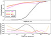 |
Fig. 1. Upper panel: completeness of the optical group catalogs based on the Magneticum mock galaxy catalog per bin of M200, FoF best proxy for R11 (red lines), T17 (orange lines), and Y05 (magenta lines) as obtained in Marini et al. (2024). The black line indicates the completeness of the X-ray selected sample extracted from the eROSITA mock observation with the eSASS detection algorithm as a function of the input M200 of Magneticum, as the X-ray selection algorithm gives no other mass proxy. Bottom panel: contamination of the optical group catalogs based on the Magneticum mock galaxy catalog per bin of original M200 of Magneticum for R11 (red lines), T17 (orange lines), and Y05 (magenta lines) as obtained in Marini et al. (2024). The black line indicates the contamination observed in the eSASS X-ray selected sample. |
These results are qualitatively consistent with those of Robotham et al. (2011). Quantitatively, the levels of completeness and contamination presented here are higher and lower, respectively, than in Robotham et al. (2011), due to the lower redshift cut (z < 0.2) of the mock galaxy sample compared to GAMA, which extends to z ∼ 0.5.
For comparison, we show also the completeness of the X-ray eSASS selection applied to the mock eROSITA observations as described in Marini et al. (2024). In this case, the completeness drops quickly to less than 50% below 1014 M⊙ and below 10% at 1013.5 M⊙, whilst the contamination increases to 20% in the same mass range.
2.1.2. The optical halo mass proxy
According to Marini et al. (2025), the best proxy for the input M200 is the total luminosity, which is converted into a mass proxy, Mlum, using the scaling relation of Popesso et al. (2005), when estimated within the same absolute magnitude range. While total stellar mass is also a good proxy, it has a slightly larger scatter. The mass derived from velocity dispersion is unreliable for groups with fewer than ten galaxy members (see Marini et al. 2025, for a more detailed analysis). Unlike velocity dispersion, total luminosity is independent of group richness and can be accurately estimated even for isolated galaxies, owing to the established correlation between central galaxy luminosity (or stellar mass) and host halo mass (Behroozi et al. 2019).
To test the robustness of the halo mass proxy Mlum from the perspective of a catalog user (e.g., as prior for the stacking analysis) we perform the following test. Since the catalog includes both true and spurious sources–with no additional information provided to the user regarding contamination levels across different observed halo mass bins–we match all detected sources in redhift and coordinates with the input catalog to evaluate the reliability of the halo mass proxy. This approach allows us to assess how well the proxy performs in practice and to quantify the impact of contaminants (i.e., spurious detections and fragmented groups) on halo mass-based analyses, such as binning systems by halo mass.
Contamination of mass proxy for the R11, T17 and Y05 catalogs.
The scatter of the Mlum − M200 relation varies with mass, being relatively small (∼0.14 dex) for Mlum > 1013.5 M⊙ and increasing up to 0.3 dex at lower values of the proxy (Fig. 2). This implies that when stacking the optically selected groups in Mlum bins, there is contamination by both lower and higher mass groups. For a fixed bin width of 0.3 dex in Mlum, this contamination increases steadily from Mlum > 1014 M⊙ to Mlum ∼ 1012.5 M⊙ for all optically selected group samples. The contamination is not symmetrical as shown in Fig. 3. The net effect, as reported in Table 1, is that a bin width of 0.3 dex in ΔMlum corresponds to an actual bin width on average of ∼0.45 for R11 and T17 and ∼0.38 dex in ΔM200 for Y05. The actual bin width is estimated as the width capturing 90% of the systems entering the ΔMlum bin. The median mass of the bin is slightly underestimated for R11. This leads to a larger contamination by more massive systems, while the opposite, a slightly larger contamination by less massive systems, is observed for T17 and Y05. This will be considered when plotting the error bars of the mean Mlum per bin in further analyses.
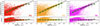 |
Fig. 2. Comparison between the input halo mass M200 and the group mass proxy based on the total luminosity scaled through the scaling relation of Popesso et al. (2005) for the three optically selected galaxy group samples: R11 (left panel), T17 (central panel) and Y05 (right panel. The solid line indicates the 1:1 relation. The green symbols indicate in all panels the mean M200 obtained in bins of 0.3 dex width of Mlum, whilst the error bars indicate the dispersion. The bottom panel shows the residuals Δ = log(Mlum)−log(M200) of the individual points and the mean values (green symbols) for the three group samples. |
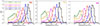 |
Fig. 3. Input halo mass M200 distribution corresponding to different bins of halo mass proxy Mlum. The left panel shows the results of the R11 group sample, the central panel the T17 group sample, and the right panel the results of the Y05 sample. The color code is indicated in the left panel. |
We also note that the largest contamination observed at MW-sized halos (Mlum ∼ 1012.5 M⊙) is mainly due to the lack of any calibration between proxies and M200 at this mass scale. Indeed, all available calibrations extend to relatively massive groups with masses larger than 1013 M⊙.
We note as a caveat that our conclusions are based only on results from the Magneticum simulation, which, while previously validated, inherently assume an accurate modeling of baryonic physics. As even small deviations in the baryon fraction can introduce significant biases in halo mass estimates, this might represent a potential limitation of the current analysis.
2.2. The synthetic eROSITA observations
The photon list of all X-ray emitting components, including hot gas, AGN, and X-ray binaries, is generated using PHOX (Biffi et al. 2012, 2013; Vladutescu-Zopp et al. 2023) for the same light cone L30 used to create the mock galaxy catalog. PHOX computes X-ray spectral emission based on the physical properties of the gas, black hole (BH), and stellar particles in the simulation. The photon list is created for all components up to a redshift z < 0.2, providing the X-ray counterpart of the galaxy mock catalog in the local Universe. As highlighted in Marini et al. (2024), which provides the detailed design of the mock observation, the adopted approach is driven by the need to include all relevant sources of contamination affecting the intra-group medium (IGrM) emission. These contaminants primarily consist of emission from active galactic nuclei (AGN) and X-ray binaries (XRBs).
AGN contamination arises in two forms: (1) detected point sources, and (2) unresolved and undetected AGN, which make up the majority of the cosmic X-ray background. To mitigate the first type, the stacking procedure systematically excludes all galaxy groups that contain a point source within their virial radius–regardless of whether the source lies in the foreground, background, or is physically associated with a group member. As a result, the fact that the light cone simulation includes only halos, galaxies, and AGN populations in the local Universe does not compromise the analysis. High-redshift AGN, which dominate the overall AGN population, would in any case be masked and excluded by the design of the stacking procedure.
The unresolved AGN population has two components: low-luminosity AGN hosted by group members, which are included in the mock observation, and high-redshift, unresolved AGN, which are accounted for in the X-ray background taken directly from the eFEDS eROSITA data. This background is added to the simulated IGrM, AGN, and XRB components.
Contamination from X-ray binaries primarily arises from star-forming galaxies located at similar redshifts and within the same region as the simulated halos. These sources are fully simulated. Any residual contribution from unresolved XRBs at higher redshift–though minor–is also included via the observed eROSITA X-ray background.
In summary, the simulated images include all significant and realistic sources of contamination, ensuring consistency with observational conditions for the stacking procedure. Further details can be found in Marini et al. (2024).
The synthetic photon lists are used as input files for the Simulation of X-ray Telescopes (SIXTE) software package (Dauser et al. 2019, v2.7.2;). SIXTE incorporates all instrumental effects, including the PSF, redistribution matrix file (RMF), and auxiliary response file (ARF) of the instrument (Predehl et al. 2021). It can also model eROSITA’s unvignetted background component due to high-energy particles (Liu et al. 2022a). We perform mock observations of eRASS:4 in scanning mode using the theoretical attitude file for the three components separately, then combine the event files. In LC30, the simulated background in all seven TMs is based on Liu et al. (2022b) and represents the spectral emission from all unresolved sources, rescaled to the eRASS:4 depth in line with the simulated emission of the individual X-ray emitting components.
The simulated eROSITA data is processed through eSASS as described in Merloni et al. (2024). The event files from all emission components and eROSITA TMs are merged and filtered for photon energies within the 0.2 − 2.3 keV band. The filtered events are binned into images with a pixel size of 4″ and 3240 × 3240 pixels. These images correspond to overlapping sky tiles of size 3.6 × 3.6 deg2, with a unique area of 3.0 × 3.0 deg2. The LC30 is covered by 122 standard eRASS sky tiles. A detailed description of the data reduction is provided in Marini et al. (2024), along with the corresponding X-ray catalog of extended and point sources (PT) provided by eSASS.
Marini et al. (2025) thoroughly analyze the completeness and contamination of the extended emission catalog, finding that, after matching the X-ray detections with the input halo catalog, the sample’s completeness drops below 80% at M200 ∼ 1014 M⊙, reaches 45% at ∼1013.5 M⊙, and no sources are detected at ∼1013 M⊙ (see Fig. 1). The contamination is negligible in the cluster mass range and is about 20% for 1013 M⊙ < M200 < 1014 M⊙.
3. The predicted eROSITA X-ray surface brightness profile
In this section, we provide the predicted emission associated with halos generated from PHOX on the L30 light cones. These predictions serve not only as benchmarks for comparison with observations but also as a basis to test the results of the stacking analysis, which underpins the observational findings.
We generate the average X-ray surface brightness profiles of all components associated with halos, including IGM, AGN, and X-ray binaries, in several halo mass bins of 0.3 dex width and convolved with the eROSITA PSF, with HEW = 30 arcsec, averaged in the 0.2–2.3 keV band (Merloni et al. 2024). The individual profiles are created in annuli of r/r200 and averaged azimuthally. Fig. 4 shows the Magneticum prediction in six halo mass bins covering the entire galaxy group mass range, from MW-type galaxy groups to poor clusters with halo masses of 1014 M⊙. Table 2 indicates the fractional contribution of each X-ray emitting component as a function of the halo mass bin.
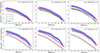 |
Fig. 4. Predicted Magneticum X-ray surface brightness profiles per bin of halo mass. The profiles are obtained by convolving the PHOX projected profiles with the eROSITA PSF. The blue-shaded regions indicate the total X-ray emission within 1σ of the mean. The magenta blue-shaded regions indicate the AGN contribution, while the gray-shaded regions indicate XRB emission. The green-shaded region indicates the IGrM emission. |
As a caveat, we note that in this analysis, we include systems in the lowest halo mass bins, with halo masses in the ranges 1012.2 − 1012.5 M⊙ and 1012.5 − 1012.8 M⊙. These are representative of MW-sized halos, corresponding to galaxies with stellar masses in the range 1010.5 − 1011 M⊙ (Behroozi et al. 2019). However, it is important to mention that the virial temperature of the gas in such low-mass halos is below the effective area of the soft band of eROSITA. Consequently, the X-ray surface brightness profiles provided here in the 0.5 − 2 keV eROSITA soft band reflect the gas at the high-temperature tail of the CGM or IGrM temperature distribution. Nonetheless, we provide this calibration due to recent eROSITA stacking results for this halo and stellar mass range (Comparat et al. 2022; Zhang et al. 2024).
As visible in Fig. 4 and quantified in Table 2, the IGrM and AGN emissions remain the main components at all halo masses. The sum of their contributions accounts for nearly the totality of the group X-ray emission. The contribution from X-ray binaries remains very low due to the low SFR values of nearby galaxies and the dominance of quenched galaxies in the local Universe. This contribution is somewhat significant (10–15%) below M200 ∼ 1013 M⊙ and becomes negligible at higher halo masses. The AGN component is the dominant component for all groups with masses below 1013 M⊙, nearly equals the IGrM contribution for groups at M200 ∼ 1013 M⊙, and becomes less significant at larger halo masses. In all cases, the contribution is primarily due to the AGN activity of the central galaxies, while the sporadic AGN activity of satellites is averaged out azimuthally.
4. Reliability of the stacking procedure
As shown in Fig. 1, the eSASS detections account for only a marginal fraction of the galaxy group population in the local Universe. From an observational perspective, accessing the average properties of the gas in groups requires stacking galaxy groups selected using different techniques. In this section, we test the results of stacking optically selected groups in the eROSITA data.
The result of any stacking procedure and its interpretation highly depends on how well the prior sample is known and characterized in terms of selection effects. Additionally, one should take into account uncertainties due to center coordinates, assumptions of gas temperature and metallicity, the halo mass proxy, and contamination by other X-ray emitting sources such as AGN and XRB.
In this case, the prior catalogs provided by the three different optically selected samples have been thoroughly analyzed in terms of completeness and contamination in Marini et al. (2024). The high level of completeness and low contamination allow the bulk of the halo population at each halo mass through stacking to be captured. Here, we analyze the effect of using optical centers, the impact of assuming an average temperature and metallicity on the gas emissivity, the contamination from other X-ray emitting sources, and the uncertainty of the halo mass proxy in the stacking procedure outlined in Popesso et al. (2024).
Briefly, the stacking is done by averaging the background subtracted surface brightness profiles within the same annuli around the group center. The background is measured in a region between 2 and 3 Mpc from the group center. All events flagged as point source in each annulus are excluded and the corresponding annulus area is corrected for the excluded point source area. All groups containing a point source or contaminated by close neighbors within 2 × r200 are excluded from the prior sample for the stacking. The X-ray luminosity from the stacked signal is derived in the 0.5–2 keV band by selecting only events with a rest frame energy in the selected band at the median redshift of the prior sample. We refer to Popesso et al. (2024) for a more detailed description of the procedure.
4.1. Effect of X-ray-optical center residuals in the stacking procedure
Figure 5 shows the distribution of the residuals ΔRA and ΔDec in kiloparsec between the X-ray center of the eSASS detections and the center of the matched halo in the input catalog. The scatter remains under 10 kpc, which is significantly smaller than the corresponding value in kiloparsec of the FWHM of the eROSITA PSF, approximately 25 arcsec, at all redshifts. These results are consistent with Seppi et al. (2022).
 |
Fig. 5. Difference in ΔRA and ΔDec, estimated in kiloparsec, between the center of the eSASS detected extended emission and the center of the input halo. |
Figure 6 shows the residuals in the center coordinates between the optically detected group center and the input halo center for the three galaxy group samples. For the majority of the R11 and Y05 groups, the center coincides with the position of the brightest group galaxy (BGG) almost at rest. Marini et al. (2025) find that all algorithms are highly efficient in identifying the BGG, with a success rate above 90% at nearly all halo masses. Due to this high efficiency, the detected optical center and the input halo coordinates coincide, with ΔRA and ΔDec close to zero. The standard deviation around the 0 residuals is approximately 15 kpc for R11, 45 kpc for T17, and 7 kpc for Y05. For the remaining 10% of cases, the residuals are below 50 kpc. The slightly larger scatter of T17 might be due to a slightly poorer performance in identifying the BCG at the high and low mass tail of the halo mass distribution, as highlighted in Marini et al. (2025).
 |
Fig. 6. Difference in ΔRA and ΔDec, estimated in kiloparsec, between the center of the detected optical group and the center of the input halo (left panel), the coordinates of the eSASS X-ray detection and the center of the input halo (central panel), and the center of the detected optical group and of the eSASS X-ray detection. |
Figure 7 shows the residuals between the X-ray and the optical center. Interestingly, the scatter of the residuals between the R11 optical center and the X-ray center is very small (less than 15 kpc). This may suggest a correlation in the deviation of the optical and X-ray centers relative to the input halo center. Although the Y05 algorithm is the most efficient in retrieving the input center, the scatter in ΔRA and ΔDec is around 50 kpc. The largest discrepancy is observed for the T17 sample, with an average residual of approximately 78 kpc.
 |
Fig. 7. Difference in ΔRA and ΔDec, estimated in kiloparsec, between the center of the detected optical group and the center of the input halo (left panel), the coordinates of the eSASS X-ray detection and the center of the input halo (central panel), and the center of the detected optical group and of the eSASS X-ray detection. |
Figure 8 illustrates the comparison between the average surface brightness profile derived by averaging the input X-ray surface brightness profiles of PHOX, convolved with the eROSITA PSF by using different centers: the input halo, and the X-ray and the optical centers. This example considers all groups simultaneously identified in the X-rays by eSASS and in the optical by the R11 algorithm, within a halo mass bin of 1013.5 M⊙ < M200 < 1013.8 M⊙. The profiles exhibit remarkable consistency. Very similar results are obtained also for the T17 and Y05 algorithms. The result demonstrates that the effect of the residuals in averaging the X-ray surface brightness profile is washed out by the large eROSITA PSF.
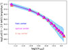 |
Fig. 8. Comparison of the average projected PHOX profiles convolved with the eROSITA PSF and centered on the input halo center (blue points), the center coordinates of the R11 mock optically selected group sample (magenta symbols), and the X-ray center (orange triangle). The shaded region indicates the overlapping 1σ region. |
Since we have not observed any effect on the input PHOX profiles, this ensures that no effects will be propagated into the stacking analysis of the mock eROSITA observations.
4.2. AGN and XRB correction to isolate the IGrM emission
As outlined in Popesso et al. (2024), all groups with a detected eSASS point source within twice r200 are discarded from the prior samples. This is done not only to mitigate the AGN contribution and isolate the IGrM component but also to clean the area around the group to properly measure and remove the background.
Using the input PHOX information, we measure the average contribution of the individual X-ray components in the mean group profile by discarding all halos with an eSASS-detected point source within 2 × r200 from the sample. These systems represent approximately 18% of the total sample. To assess whether excluding this subpopulation affects the stacking results, we compare the average contribution of individual X-ray components within r200 for the full sample and for the sample cleaned of groups contaminated by point sources. The results of this comparison are shown in Table 2. We find that the difference in average values between the full and clean samples is negligible. This is expected, as most of the detected point sources are located in the foreground or background and are rarely (< ∼ 3% of cases) physically associated with group members. This confirms that the exclusion of the groups contaminated by point sources should not affect our conclusion on the average properties of undetected groups. Additionally, it indicates also that the primary source of contamination is not the relatively bright AGN detected by eSASS in our eRASS:4-like mock observations. Rather, the contamination is entirely due to AGN fainter than the eRASS:4 detection threshold that are hosted by group galaxies.
We observe that discarding groups with a PT within 2 × r200 leads to lowering the noise of the background measurement. Indeed, removing PT enables us to improve the accuracy of the background estimate by 35%. We conclude that removing halos contaminated by PT detections has a marginal effect on mitigating AGN contamination but is essential to increase the accuracy of the background estimate.
Nevertheless, correcting for AGN and XRB contamination is essential to properly isolate the IGrM contribution. This can only be done by modeling the halo occupation distribution and the conditional X-ray luminosity function of the AGN population. Many models are available for the halo occupation distribution of AGN at different redshifts (e.g., Georgakakis et al. 2019; Krumpe et al. 2018; Aird & Coil 2021; Powell et al. 2022; Krumpe et al. 2023; Comparat et al. 2023). These models can reproduce the clustering properties and the X-ray luminosity function of the observed AGN population fairly well. However, all models are constrained either by observations at higher redshifts (e.g., Georgakakis et al. 2019; Aird & Coil 2021; Comparat et al. 2023) or by relatively bright local AGN (e.g., Krumpe et al. 2018; Powell et al. 2022). Thus, they require extrapolation to lower redshift, as in our case (z < 0.2), or to lower luminosities. Since there is no easy way to discern which model performs better in this parameter range, we rely on the Magneticum results. Indeed, Hirschmann et al. (2014) show that the AGN model implemented in Magneticum can broadly match observed black hole properties of the local Universe, including the observed soft and hard X-ray luminosity functions of AGN and clustering properties. Marini et al. (2024) also shows that the analysis of the eRASS:4-like mock observations based on the Magneticum light cones reproduces well the soft X-ray AGN luminosity function of Marchesi et al. (2020). We thus correct the X-ray surface brightness profile obtained through the stacking analysis by subtracting a PSF with a signal equal to the percentage of X-ray luminosity due to AGN contamination per halo mass bin, as indicated in Table 2.
Contribution of emitting sources in halos per halo mass bin.
To remove the residual XRB contamination, we apply the following approach. The XRB contribution, in nearly all cases, is due to the mean SFR of the central galaxies. Satellite galaxies in the local Universe tend to be quiescent or highly quenched, occupying regions well below the Main Sequence (MS) of star-forming galaxies (Popesso et al. 2019). Thus, their SFR activity contributes very little to the XRB emission, becoming negligible when averaged azimuthally to obtain the surface brightness profile. Central galaxies in MW-sized halos, on the other hand, tend to be MS galaxies, as shown in Popesso et al. (2019). Therefore, since in most cases, the optical center coincides with the central galaxy location, the XRB contribution due to the star formation activity of the central galaxy can be modeled by a PSF rescaled to reproduce the X-ray luminosity of this contribution.
To estimate this, we use the scaling relation from Lehmer et al. (2016), which links the X-ray luminosity in the 0.5–2 keV band to the galaxy SFR. We use the mean SFR of the central galaxies in each halo mass bin to estimate the corresponding mean X-ray luminosity. We then subtract a PSF rescaled to this luminosity from the stacked profile to remove the IGrM contribution. This approach nicely reproduces the same level of XRB contamination estimated through PHOX in each halo mass bin.
4.3. The group X-ray emissivity
The X-ray emissivity is the energy emitted per time and volume by the hot gas in galaxy systems, typically described as an optically thin plasma in collisional ionization equilibrium. This is a key element when deriving the gas mass profile from the X-ray surface brightness profile of halos. The emissivity is defined as npneΛ(T, Z), where np and ne are the proton and electron densities, respectively, and Λ(T, Z) is the gas cooling function, which depends on the emission process, gas temperature, and metallicity. As shown in Lovisari & Ettori (2021), at temperatures higher than approximately 3 keV, the main emission mechanism is thermal bremsstrahlung. At this scale, the emissivity in the 0.5–2 keV band considered here is nearly independent of temperature and metallicity. However, at lower temperatures, within the group regime, line cooling becomes significant, and the emissivity strongly varies as a function of metallicity and temperature.
The temperature and metallicity of the hot gas in galaxy groups can only be measured by modeling the gas X-ray spectrum and its emission lines. However, this information is not available for the undetected systems in the optically selected prior catalog. Thus, to estimate the emissivity and derive the hot gas mass profile from the observed X-ray surface brightness profile, we must assume a mean temperature and metallicity. While an average temperature for groups can be derived from existing scaling relations (see Lovisari et al. 2015; Lovisari & Ettori 2021), very little is known about the global distribution and average gas metallicity, as well as the shape of possible spatial gradients in low-mass systems (see also Sun et al. 2009; Mernier et al. 2017; Lovisari & Reiprich 2019).
In this analysis, we assume a mean temperature derived from the group halo mass proxy using the Lovisari et al. (2015)M − TX scaling relation, similar to how we would handle real observations. This assumption is justified for our eROSITA mock observations because Magneticum simulations accurately reproduce the Lovisari et al. (2015)M − TX scaling relation, as shown in Marini et al. (2024). We assume a mean metallicity of 0.3 Z⊙ for all groups and neglect any temperature and metallicity profiles within the groups, although they are present in the Magneticum X-ray groups. As shown in Fig. 9, the assumption of 0.3 Z⊙ is reasonable for the Magneticum simulation. The figures shows the distribution of mass-weighted metallicity estimated from the hot gas particles in the simulation within r500 per halo mass bin. This slightly varies from 0.17 Z⊙ at approximately 3 × 10¹² M⊙ to 0.37 Z⊙ at approximately 1014 M⊙, but the trend is poorly significant. Additionally, we point out that the gas metallicities at the group mass scale treated here, from MW-sized halos to massive groups, are very poorly constrained and measured only in X-ray-selected groups, which might provide a biased picture.
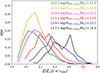 |
Fig. 9. Distribution of the mass-weighted metallicity of the Magneticum halos estimated within r500 in different halo mass bins. The histograms are color coded as described in the figure according to the halo mass bin. |
The upper panels of Fig. 10 compare the input mass-weighted temperature measured from the hot gas particles in the simulation within r500 with the temperature derived from the best halo mass proxy based on the total luminosity of each prior catalog. The temperature proxy agrees well with the input temperature for the R11 catalog. The T17 and Y05 catalogs tend to largely underestimate the temperature below to 0.25 keV and overestimate above this threshold by 20–30%. This aligns with the slight underestimation of the halo mass proxy compared to the input halo mass for the T17 and Y05 catalogs, as shown in Fig. 2. We note that some level of discrepancy is expected, as the M–TX scaling relation used to derive temperature from mass is not fully consistent with the relation found in the Magneticum simulation, as discussed in Marini et al. (2024). The lower panel of the same figure shows how this effect translates into an error in the X-ray emissivity. The red curve in the plot shows the emissivity estimated in the 0.5–2 keV band, assuming a fixed metallicity of 0.3 Z⊙ as in Asplund et al. (2009). The green points indicate, for each prior catalog, the effect on the emissivity at the same metallicity and energy band based on the temperature mass proxy. For the R11 catalog, the use of the temperature proxy leads to a percentage uncertainty in the X-ray emissivity of 23% without evident systematics. For the T17 and Y05 catalogs, the net effect is an overestimation of 20% and 27% of the emissivity below 0.6 keV and an underestimation of approximately 10% between 0.8 and 1.6 keV. Nearly the same values are found at higher metallicity, while at lower values, the effect is marginal in all cases.
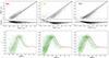 |
Fig. 10. Upper panels: relation between the input mass-weighted gas temperature derived within r500 for the Magneticum halos and the temperature derived from the optical halo mass proxy through the scaling relation of Lovisari et al. (2015) for each prior catalog: R11 (left panel), T17 (central panel), and Y05 (right panel). Each panel also shows the residuals in dex as a function of the gas temperature proxy. Bottom panels: expected temperature–emissivity relation, at fixed metallicity (0.3 Z⊙), estimated at the input mass-weighted gas temperature derived within r500 for the Magneticum halos and the X-ray emissivity (red curve in each panel). The green points indicate the emissivity corresponding to the temperature proxy obtained from the optical halo mass proxy of the different optically selected group samples (R11 left panel, T17 central panel, and Y05 right panel) and estimated for the same metallicity. |
For the sake of this experiment, such variation in metallicity has only a minor effect on the mean emissivity per halo mass bin. Indeed, the effect of the temperature proxy uncertainty is larger. Thus, the assumption of a 0.3 Z⊙ metallicity is reliable. However, we point out that a larger spread might be present in the observed groups.
4.4. The uncertainty of the halo mass proxy
To test the effect of uncertainty in the halo mass proxy, we measured the average PHOX profiles convolved with the eROSITA PSF, binned by halo mass based on the halo mass proxy of different samples.
The retrieved IGrM contribution is shown for each halo mass proxy bin and prior catalog in Fig. 11 and compared with the predicted IGrM profile from Magneticum as shown in Fig. 4. The following results were observed:
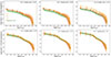 |
Fig. 11. Comparison in different halo mass bins between the PHOX input IGrM profiles convolved with the eROSITA PSF and averaged in input halo mass bins (green shaded region), with profiles averaged in halo mass proxy bins (colored symbols). The green-shaded region indicates the 1σ error. The colored points show the mean PHOX profiles obtained from the different prior catalogs (yellow for R11, orange for T17, and gold for Y05). The error bars indicate the 1σ uncertainty. |
At halo mass proxies below 1013 M⊙ (top three panels in Fig. 11), the IGrM surface brightness profile is consistently overestimated by a factor that varies depending on the prior catalog. This effect is due to the lack of reliable calibration of the halo mass proxy at this scale and the large scatter in the correlation, as highlighted in Fig. 3 and Table 1. Results based on the R11 prior sample exhibit a larger discrepancy, particularly in the 1012.8 − 1013.1 M⊙ halo mass proxy bin. This is likely due to significant contamination from higher mass halos in the bin defined by the halo mass proxy, as shown in Table 1.
At halo mass proxies above 1013 M⊙ (bottom three panels in Fig. 11), the IGrM surface brightness profile is in remarkable agreement with the input surface brightness profile across all three prior samples. We do not observe any significant discrepancies due to the halo mass proxy at this mass scale because the scatter in the proxy calibration is much smaller than at lower masses. Additionally, contamination by lower and higher mass halos decreases by a factor of 2 compared to the lower mass bins (see Table 1), and the contamination tends to be more symmetrical to the bin center (see Fig. 3).
4.5. The stacking results
We test the efficiency of the stacking procedure in retrieving the input IGrM surface brightness profile (see Fig. 4) using the three optically selected group samples analyzed here. The stacking is performed at the coordinates of the optically selected group samples and within halo mass bins determined by each sample’s halo mass proxy. The X-ray emissivity is based on the temperature proxy derived from the mass–temperature relation, as described above, assuming a 0.3 Z⊙ metallicity. The effects of the assumed temperature and metallicity are included in the error budget by summing in quadrature the error estimated via bootstrapping and the effects estimated at different halo mass bins in previous sections. AGN contamination is removed by following the predictions from the simulation estimated in Table 2, while XRB contamination is removed using the Lehmer et al. (2016) scaling relation in the 0.5–2 keV band. The effect of using the optical halo mass proxy is not corrected for, but it will be discussed here.
Figure 12 shows the comparison between the retrieved stacked IGrM X-ray surface brightness profiles based on the three different optical prior catalogs and the input average PHOX IGrM profile obtained in bins of input halo mass as in Fig. 5.
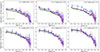 |
Fig. 12. Comparison in different halo mass bins between the PHOX input IGrM profiles convolved with the eROSITA PSF and the results of the stacking procedure on the mock observations. The PHOX profiles are averaged in bins of input halo mass, while the stacked profiles are obtained in bins of halo mass proxy of the related prior catalog (blue for R11, violet for T17, and pink for Y05). |
Despite the large error bars due to the aforementioned effects and the background subtraction, particularly at radii larger than ∼0.7 − 0.9r200, the stacked profiles exhibit remarkably good agreement. The only evident effect is an overestimation of the R11-based stacked profile in the halo mass proxy bin at 1012.8 − 13.1 M⊙, which was also observed in Fig. 11 and is due to the large contamination of high mass halos at halo masses larger than the bin’s upper limit.
The results demonstrate that the stacking procedure can accurately reproduce the average input profile derived from averaging the PHOX profiles of the underlying halo population at the same mass. This implies that:
-
i) The optical selection effectively captures the average properties of the parent halo population.
-
ii) The stacking procedure performs proper background subtraction and accurately captures the shape of the input X-ray surface brightness profile up to r200.
-
iii) The group center location does not statistically affect the profile shape, as the uncertainty is significantly smaller than the FWHM of the PSF, and any differences are mitigated by PSF convolution.
-
iv) The assumed temperature and metallicity do not significantly affect the derived profile but should be considered in the error budget.
-
v) Ignoring any temperature and metallicity spatial profiles does not dramatically affect the shape of the retrieved X-ray surface brightness profile.
-
vi) The main source of uncertainty derives from using the optical halo mass proxy, particularly when contamination is significant. Nevertheless, this seems to affect only a single bin and a single prior catalog.
Therefore, we conclude that utilizing the optically selected sample as a prior catalog for the stacking procedure defined in Popesso et al. (2024) yields a reliable and robust estimate of the average X-ray surface brightness profile of galaxy groups when all selection and contamination effects are considered.
4.6. The reconstruction of the gas mass profile
The X-ray surface brightness profile carries information on how the hot gas is distributed in halos. The hot gas mass profile is usually reconstructed from the X-ray surface brightness profile, by assuming and electron density model. Here we use the Vikhlinin et al. (2006) electron number density model, as usually done in the literature (see also Liu et al. 2022a; Bulbul et al. 2024):
 (1)
(1)
where n0 is the normalization factor, rc and rs are the core and scale radii, β controls the overall slope of the density profile, α controls the slope in the core and at intermediate radii, and ϵ controls the change of slope at large radii. This is used to estimate and integrate along the line of sight the X-ray emissivity, ne(r)2Λ(kT, Z) profile, where Λ(kT, Z) is the cooling function depending on the gas temperature and metallicity. To mimic the observational technique, we estimate the cooling function by assuming a gas temperature from the M − TX relation of Lovisari et al. (2015) at the mean M500 of the halo mass (proxy) bin. As in Liu et al. (2022a), we assumed a metallicity of the ICM of 0.3 Z⊙, adopting the solar abundance table of Asplund et al. (2009), that includes the He abundance. We neglect any temperature and metallicity profile. The projected number density model is convolved with the eROSITA PSF and fitted to the data to retrieve the best-fit parameters.
Figure 13 presents the electron density profile predicted by the Magneticum simulation for a random subsample of halos across six halo mass bins. This is compared to the best-fit electron number density model from Vikhlinin et al. (2006), derived from fitting the stacked X-ray surface brightness profiles in Figure 12. We display the best-fit model for each mock, optically selected galaxy group sample. Despite substantial uncertainties in emissivity due to assumptions about mean gas temperature and metallicity, the profile obtained through the stacking method accurately reproduces the input average profiles.
 |
Fig. 13. Comparison in different halo mass bins between the electron density profiles predicted by Magneticum (light pink points and solid curves) and the best-fit profiles obtained from the stacked X-ray surface brightness profiles of Fig. 12 of the three optical group catalogs of R11 (blue curve), Y05 (magenta curve) and T17 (purple curve). |
5. Comparison with observed IGrM profiles
Here we provide a comparison between the predicted Magneticum IGrM profiles and the one recently obtained from the eROSITA survey and based on the stacking analysis.
Fig. 14 presents the comparison between the average PHOX IGrM profiles of Fig. 4 and the observed stacked profiles obtained in Popesso et al. (2025) by following the same stacking technique tested here and based on the real R11 GAMA optically selected group sample. The observed stacked profiles are obtained in halo mass bins based on the total luminosity halo mass proxy tested here. The AGN and XRB contamination are corrected also in the real data as explained in Section 4.2. In all cases, the predicted PHOX profiles agree within 1–1.5σ with the observed profiles. We observe the largest discrepancy in the highest mass bins where we have the lowest number of systems, due to the limited volume, and the largest uncertainty.
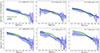 |
Fig. 14. Comparison in different halo mass bins between the PHOX input IGrM profiles convolved with the eROSITA PSF (green-shaded region) and the observed stacked profiles of Popesso et al. (2025, blue-shaded region). The latter profiles were obtained by following the same stacking procedure used here and with the real R11 GAMA optically selected group catalog. The shaded regions indicate the 1σ uncertainty. |
Fig. 15 presents a comparison of the PHOX IGrM profiles (shown in Fig. 4) with the observed stacked profiles from Zhang et al. (2024), derived from the optically selected group catalog of Tinker (2021, hereafter T21). As shown in Fig. 15, the observed profiles do not align with either the Magneticum predictions or the results from Popesso et al. (2025). The primary cause of this discrepancy is the use of different halo mass proxies in the T21 and R11 optical group prior catalogs. Despite both methods applying corrections for AGN contamination and satellite X-ray background (XRB), the underlying issue is a systematic underestimation of X-ray flux in the stacked profiles prior to these corrections, as highlighted in Zhang et al. (2024). This discrepancy is likely attributable to differences in how the halo mass proxy is defined and estimated.
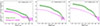 |
Fig. 15. Comparison in different halo mass bins between the PHOX IGrM input profiles convolved with the eROSITA PSF and the observed stacked profiles of Zhang et al. (2024, magenta-shaded region). The latter profiles were obtained by following the stacking procedure outlined in Zhang et al. (2024) and with the real Tinker (2021) optically selected group catalog in the SDSS area. The shaded regions indicate the 1σ uncertainty. |
To investigate this further, we compare the T21 halo mass proxy with the Y05 estimates over the SDSS area, as both algorithms use the same dataset (see appendix). Both rely on total optical luminosity to estimate halo mass via a calibration, but T21 adopts a more complex calibration that depends on galaxy properties (e.g., color), whereas Y05 uses a single power law. A direct comparison of the T21 and Y05 halo mass proxies reveals discrepancies in both the total luminosity estimates and the resulting halo masses (see Fig. A.1). Given that Marini et al. (2025) extensively tested the Y05 algorithm for accurately identifying central and member galaxies and reliably estimating halo masses, we conclude that misidentifications in group membership, coupled with a less accurately tested calibration in T21, likely lead to an over-representation of low-mass, low-X-ray luminosity groups in the T21 catalog at fixed halo masses (see Fig. A.2). This, in turn, results in a reduced mean X-ray flux in the stacked profiles.
This finding emphasizes the importance of carefully considering the halo mass proxy and selection biases in the prior catalog, as these factors significantly influence the outcomes of X-ray stacking analyses (see appendix for further details).
6. Scaling relations
6.1. The LX–mass relation down to MW sized halos
We present the predicted LX–mass relation based on the stacking analysis of the Magneticum-eROSITA mock observation, using the three optically selected prior catalogs considered in this study. Marini et al. (2024) have already shown that the LX–mass relation predicted by Magneticum is consistent with the available observational relations, calibrated down to halo masses of M500 ∼ 1013.5 M⊙ (see e.g., Pratt et al. 2010; Lovisari et al. 2015; Chiu et al. 2022). Here, we demonstrate in Fig. 16 that this relation can be accurately retrieved by our stacking analysis. The stacked relations were derived by integrating the stacked profiles from Fig. 12 within r500. Additionally, we include a data point for clusters with M500 > 1014 M⊙. Nearly all optically selected clusters have been detected as eSASS extended sources.
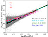 |
Fig. 16. LX–mass relation in the 0.5 − 2.0 keV band based on the stacking analysis applied to the Magneticum-eROSITA mock observations and based on the R11, T17 and Y05 optically selected galaxy group catalog. The relations are color coded as outlined in the figure: orange for R11, magenta for T17, and red for Y05 prior catalogs, respectively. The black symbols indicate the mean relation of the input Magneticum halos, while the black solid line indicates the best-fit obtained by considering input X-ray luminosity and mass for halos with M500 > 1013.5 M⊙. The cyan solid line indicates the relation of Pratt et al. (2009). The green solid line shows the relation of Lovisari et al. (2015) and the blue line the one of Chiu et al. (2022) in the 0.5 − 2.0 keV band. |
All stacked points, irrespective of the group selection algorithm, result in flatter LX–mass relations compared to the input relation, with the greatest discrepancies observed in the lowest halo mass bins, as shown in Fig. 12. According to our analysis of potential sources of systematic errors and uncertainties discussed in the previous sections, this discrepancy is primarily due to the halo mass proxy used for binning the prior samples. Specifically, we employed the same proxy across all three catalogs, the group total optical luminosity, which is poorly calibrated for halo masses below 1013 M⊙. Any systematic errors in this calibration (see Table 1) propagate as systematic errors in the LX–mass slope. Therefore, caution should be exercised when comparing the LX–mass slope obtained from stacked scaling relations with other studies in the literature that utilize different halo mass proxies and predictions.
6.2. The fgas − M500 relation down to MW sized halos
The fgas − M500 relation is a key to understand how much hot gas is locked in massive halos within a given radius. Here we focus on the relation estimated within r500. The mass of the hot gas within each halo mass bin is estimated by integrating the best-fit electron number density model from Vikhlinin et al. (2006) obtained in Fig. 13. The gas mass within r500 is normalized to the M500 estimate based on mass proxy of the corresponding optically selected sample used as prior for the stacking. The predicted relation from Magneticum is, instead, calculated by averaging the predicted hot gas mass fraction within a halo mass bin. This is estimated by considering all gas particle with a tempertaure higher than 105 K.
Fig. 17 shows the comparison between the Magneticum prediction and the relation based in the stacked profiles. The error bars for the Magneticum prediction represent the dispersion around the mean, while the error bars of the gas fraction based on the stacks are obtained by summing in quadrature the error of the best-fit due to the observed error in the stacked surface brightness profiles and the uncertainty due to the assumption of the mean gas temperature and metallicity in the emissivity (see Section 4.3). The input predictions and those retrive by applying the observational technique to the mock dataset are perfectly in agreement within the error bars. This ensures that the stacking technique is capable of retrieving the input average properties of the underlying halo population.
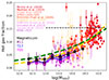 |
Fig. 17. fgas − M500 relation. The filled circles represent a compilation of literature data, color coded as a function of the sample reference as shown in the picture. The black points connected by a solid line represent the Magneticum prediction. The squares indicate the fgas derived from the stacked X-ray surface brightness profiles. This is obtained by integrating the best-fit electron density model of Fig. 13. The dashed yellow and green curves represent the best-fit of Pratt et al. (2009) and Eckert et al. (2016), respectively. The dashed line indicates the value of the cosmic baryon fraction according to the WMAP cosmology implemented in Magneticum. |
In addition, in Fig. 17 we also show a comprehensive compilation of literature data providing the same estimate for z < 0.2 systems. These are the cluster sample of Mulroy et al. (2019), Mahdavi et al. (2013), Eckert et al. (2019), the REXCESS sample of Pratt et al. (2009), the poor cluster and group sample of Arnaud et al. (2007), Vikhlinin et al. (2006), and Sun et al. (2009) used in Pratt et al. (2009) (APP05+V09+S09 in Fig. 17), the XMM-XXL sample of Eckert et al. (2016), the group samples of Gonzalez et al. (2013) and Lovisari et al. (2015), the poor cluster sample of Ragagnin et al. (2022), and the group sample of Rasmussen & Ponman (2009) and Pearson et al. (2017) (RP09+P17 in Fig. 17). We transformed all the values into our adopted cosmology. Given the very different selection functions of the collected data, it is not surprising that the scatter is large. Nevertheless, we find consistency in the distribution of the observed systems and the mean prediction of Magneticum in the group and poor cluster regimes.
7. Discussion and conclusions
The creation of eROSITA mock observations at the eRASS:4 depth and optical galaxy catalogs based on the same Magneticum lightcones in the local Universe (see Marini et al. 2024) allowed us to generate synthetic analogs that mirror the available observational datasets. These datasets are created by combining eROSITA observations with optically selected catalogs such as those by Robotham et al. (2011) in the GAMA area, and Tempel et al. (2017) and Yang et al. (2005) in the SDSS region. We created synthetic analogs of optically selected group catalogs using the selection algorithms from these three reference papers.
We present a thorough analysis of the sources of systematic errors and uncertainties involved in the stacking analysis of optically selected groups in the eROSITA data. In particular, we test the impact of these systematics and uncertainties on the results of the stacking technique by Popesso et al. (2019), applied to the three synthetic optically selected group catalogs considered here. Following the findings of Marini et al. (2024), we use the total optical group luminosity as a halo mass proxy, which exhibits the least scatter when compared with the input halo mass. We discuss the following:
-
The completeness and contamination of the prior optical group catalogs and the effect of any selection biases.
-
The effect of possible optical miscentering when stacking at the coordinates of the optically selected groups.
-
The impact on X-ray emissivity estimation when assuming a temperature based on the TX–mass scaling relation through the halo mass proxy, and a fixed metallicity (0.3 Z⊙).
-
The contamination from AGN and XRB emission.
-
The effect of the scatter between the halo mass proxy and the input halo mass on the contamination within each halo mass bin.
To test these effects, we constructed predicted contributions to the X-ray emission in different halo mass bins and projected X-ray surface brightness profiles. We isolated the IGrM contribution in each halo mass bin and evaluated how effectively the stacking procedure retrieves the input IGrM surface brightness profile. This analysis includes halos with masses below 1013 M⊙. However, we note that the mean virial temperature of the hot gas in such halos is below the energy range of the eROSITA soft band. Therefore, the provided predictions of the IGrM profiles in these halo mass bins only reflect the gas particles in the high-temperature tail of the gas temperature distribution. Consequently, these predictions are not representative of the entire CGM or IGrM emission in low-mass systems.
The analysis leads to the following results:
-
The completeness and contamination of the prior optical group catalogs are such that no significant selection effects are observed.
-
The differences in coordinates (ΔRA and ΔDec) between the input halo center and the optical center are much smaller than the eROSITA PSF at the considered redshifts. Therefore, any mis-centering effect is mitigated when the Magneticum projected PHOX X-ray surface brightness profiles are convolved with the eROSITA PSF. We do not observe significant mis-centering relative to the X-ray center in the eSASS extended source detections matched to the input and optically selected group catalogs.
-
The effect on X-ray emissivity depends on the systematics of the halo mass proxy. If this proxy is used to infer the mean temperature of the gas from the TX–mass relation, the temperature can be over- or underestimated. For the R11 catalog, the total luminosity proxy results in a scatter of 40% in the emissivity estimate at fixed metallicity. For the T17 and Y05 catalogs, we observe an overestimation of approximately 20% below 0.6 keV and an underestimation of 10% above this threshold. The assumption of a fixed metallicity of 0.3 Z⊙ aligns relatively well with the Magneticum simulation, as 85% of the halos in the two orders of magnitude in halo mass considered here exhibit a mean metallicity in the range 0.1 − 0.45 Z⊙, leading to a variation in emissivity of 37%. Since these effects cannot be corrected when estimating the electron number density profile and gas mass, they are included in the error budget and summed in quadrature with the error due to background subtraction.
-
According to the Magneticum predictions, AGN contamination dominates the X-ray surface brightness profile emission in all halos with masses below 1013 M⊙, which contain the majority of low X-ray luminosity AGN. Consistent with Popesso et al. (2024), AGN contamination is limited to the activity of the central galaxy and is well modeled with a PSF rescaled to the percentage of the X-ray emission corresponding to the AGN contribution. Similarly, XRB contamination is mainly due to the central galaxy’s activity and is significant on average only for halos with masses below 1013 M⊙, while it can be neglected for more massive halos. This contamination can also be modeled as a PSF and subtracted from the total X-ray emission.
-
The most significant systematic effect in the stacking analysis is the scatter between the halo mass proxy and the input halo mass. Each halo mass bin sample might be differently contaminated by high and low mass systems depending on the level of agreement between the halo mass proxy and the input mass. This systematic leads to an overall overestimation of the X-ray surface brightness profiles, particularly for halos with masses below 1013 M⊙.
-
When performing the stacking analysis in the mock observations, all these effects tend to compensate for each other to some extent. We confirm an overestimation of the X-ray surface brightness profile for low mass groups below 1013 M⊙ mainly due to contamination in the bins of the halo mass proxy. For halos with masses above 1013 M⊙, we find good agreement between the stacked and input projected PHOX profiles.
-
Any systematic error in the calibration of the halo mass proxy is propagated when estimating the scaling relations based on the stacks. This is more visible in the LX−mass relation. We show the relations based on the stacking of the different optically selected group priors and find that, in all cases, the slope of the relations is flatter than the input relation. Such systematic errors must be considered when comparing the results of any stacking technique with other works in the literature based on different prior catalogs, detections, or predictions.
The comparison of the Magneticum input IGrM PHOX profiles with the observed profiles of Popesso et al. (2025) shows that the predictions align well with the observations. However, when these results are compared with the X-ray surface brightness profile from Zhang et al. (2024), a discrepancy is noted across all considered halo masses, with the corresponding flux level being lower than that of Magneticum and the observed LX–mass relation (e.g., Pratt et al. 2009; Lovisari et al. 2015; Chiu et al. 2022). This discrepancy highlights the impact of systematics in the stacking analysis, which can lead to differences when comparing results based on different prior samples and techniques.
We conclude that overall, the stacking technique is reliable when all systematics are properly considered and corrected where possible. If a correction is not feasible, the uncertainty should be included in the error budget. Once the selection effects of the optical selection algorithms are properly checked, the main source of systematics and uncertainty remains the halo mass proxy chosen for the binning in halo mass. Using the best proxy with the smallest scatter compared to the input halo mass, namely the total optical luminosity, still leads to some contamination in the lowest halo mass bins, which can affect the study of the slope of the LX–mass relation. Overall, Magneticum predictions are consistent with observations of scaling relations and can accurately reproduce the observed X-ray surface brightness profiles over the two decades of halo masses in the group regime below 1014 M⊙.
Acknowledgments
PP acknowledges financial support from the European Research Council (ERC) under the European Union’s Horizon Europe research and innovation programme ERC CoG CLEVeR (Grant agreement No. 101045437). AB acknowledges the financial contribution from the INAF mini-grant 1.05.12.04.01 “The dynamics of clusters of galaxies from the projected phase-space distribution of cluster galaxies”. KD acknowledges support by the COMPLEX project from the European Research Council (ERC) under the European Union’s Horizon 2020 research and innovation program grant agreement ERC-2019-AdG 882679. The calculations for the Magneticum simulations were carried out at the Leibniz Supercomputer Center (LRZ) under the project pr83li. GP acknowledges financial support from the European Research Council (ERC) under the European Union’s Horizon 2020 research and innovation program Hot- Milk (grant agreement No 865637), support from Bando per il Finanziamento della Ricerca Fondamentale 2022 dell’Istituto Nazionale di Astrofisica (INAF): GO Large program and from the Framework per l’Attrazione e il Rafforzamento delle Eccellenze (FARE) per la ricerca in Italia (R20L5S39T9). SVZ and VB acknowledge support by the Deutsche Forschungsgemeinschaft, DFG project nr. 415510302 This work is based on data from eROSITA, the soft X-ray instrument aboard SRG, a joint Russian-German science mission supported by the Russian Space Agency (Roskosmos), in the interests of the Russian Academy of Sciences represented by its Space Research Institute (IKI), and the Deutsches Zentrum für Luft- und Raumfahrt (DLR). The SRG spacecraft was built by Lavochkin Association (NPOL) and its subcontractors and is operated by NPOL with support from the Max Planck Institute for Extraterrestrial Physics (MPE). The development and construction of the eROSITA X-ray instrument was led by MPE, with contributions from the Dr. Karl Remeis Observatory Bamberg & ECAP (FAU Erlangen-Nuernberg), the University of Hamburg Observatory, the Leibniz Institute for Astrophysics Potsdam (AIP), and the Institute for Astronomy and Astrophysics of the University of Tübingen, with the support of DLR and the Max Planck Society. The Argelander Institute for Astronomy of the University of Bonn and the Ludwig Maximilians Universität Munich also participated in the science preparation for eROSITA. The eROSITA data shown here were processed using the eSASS software system developed by the German eROSITA consortium.
References
- Aird, J., & Coil, A. L. 2021, MNRAS, 502, 5962 [NASA ADS] [CrossRef] [Google Scholar]
- Alpaslan, M., & Tinker, J. L. 2020, MNRAS, 496, 5463 [NASA ADS] [CrossRef] [Google Scholar]
- Anderson, M. E., Gaspari, M., White, S. D. M., Wang, W., & Dai, X. 2015, MNRAS, 449, 3806 [NASA ADS] [CrossRef] [Google Scholar]
- Arnaud, M., Pointecouteau, E., & Pratt, G. W. 2007, A&A, 474, L37 [CrossRef] [EDP Sciences] [Google Scholar]
- Asplund, M., Grevesse, N., Sauval, A. J., & Scott, P. 2009, ARA&A, 47, 481 [NASA ADS] [CrossRef] [Google Scholar]
- Beck, A. M., Murante, G., Arth, A., et al. 2016, MNRAS, 455, 2110 [Google Scholar]
- Behroozi, P., Wechsler, R. H., Hearin, A. P., & Conroy, C. 2019, MNRAS, 488, 3143 [NASA ADS] [CrossRef] [Google Scholar]
- Biffi, V., Dolag, K., Böhringer, H., & Lemson, G. 2012, MNRAS, 420, 3545 [NASA ADS] [Google Scholar]
- Biffi, V., Dolag, K., & Böhringer, H. 2013, MNRAS, 428, 1395 [Google Scholar]
- Biffi, V., Dolag, K., & Merloni, A. 2018, MNRAS, 481, 2213 [Google Scholar]
- Bulbul, E., Liu, A., Kluge, M., et al. 2024, A&A, 685, A106 [NASA ADS] [CrossRef] [EDP Sciences] [Google Scholar]
- Chiu, I. N., Ghirardini, V., Liu, A., et al. 2022, A&A, 661, A11 [NASA ADS] [CrossRef] [EDP Sciences] [Google Scholar]
- Clerc, N., Ramos-Ceja, M. E., Ridl, J., et al. 2018, A&A, 617, A92 [NASA ADS] [CrossRef] [EDP Sciences] [Google Scholar]
- Comparat, J., Truong, N., Merloni, A., et al. 2022, A&A, 666, A156 [NASA ADS] [CrossRef] [EDP Sciences] [Google Scholar]
- Comparat, J., Luo, W., Merloni, A., et al. 2023, A&A, 673, A122 [NASA ADS] [CrossRef] [EDP Sciences] [Google Scholar]
- Dauser, T., Falkner, S., Lorenz, M., et al. 2019, A&A, 630, A66 [NASA ADS] [CrossRef] [EDP Sciences] [Google Scholar]
- Di Matteo, T., Springel, V., & Hernquist, L. 2005, Nature, 433, 604 [NASA ADS] [CrossRef] [Google Scholar]
- Dolag, K., Vazza, F., Brunetti, G., & Tormen, G. 2005, MNRAS, 364, 753 [NASA ADS] [CrossRef] [Google Scholar]
- Dolag, K., Borgani, S., Murante, G., & Springel, V. 2009, MNRAS, 399, 497 [Google Scholar]
- Dolag, K., Komatsu, E., & Sunyaev, R. 2016, MNRAS, 463, 1797 [Google Scholar]
- Eckert, D., Ettori, S., Coupon, J., et al. 2016, A&A, 592, A12 [NASA ADS] [CrossRef] [EDP Sciences] [Google Scholar]
- Eckert, D., Ghirardini, V., Ettori, S., et al. 2019, A&A, 621, A40 [NASA ADS] [CrossRef] [EDP Sciences] [Google Scholar]
- Eckert, D., Gaspari, M., Gastaldello, F., Le Brun, A. M. C., & O’Sullivan, E. 2021, Universe, 7, 142 [NASA ADS] [CrossRef] [Google Scholar]
- Erfanianfar, G., Finoguenov, A., Furnell, K., et al. 2019, A&A, 631, A175 [NASA ADS] [CrossRef] [EDP Sciences] [Google Scholar]
- Erfanianfar, G., Popesso, P., Finoguenov, A., et al. 2014, MNRAS, 445, 2725 [Google Scholar]
- Fabjan, D., Borgani, S., Tornatore, L., et al. 2010, MNRAS, 401, 1670 [Google Scholar]
- Georgakakis, A., Comparat, J., Merloni, A., et al. 2019, MNRAS, 487, 275 [NASA ADS] [CrossRef] [Google Scholar]
- Gonzalez, A. H., Sivanandam, S., Zabludoff, A. I., & Zaritsky, D. 2013, ApJ, 778, 14 [Google Scholar]
- Haardt, F., & Madau, P. 2001, ArXiv e-prints [arXiv:astro-ph/0106018] [Google Scholar]
- Hirschmann, M., Dolag, K., Saro, A., et al. 2014, MNRAS, 442, 2304 [Google Scholar]
- Krumpe, M., Miyaji, T., Coil, A. L., & Aceves, H. 2018, MNRAS, 474, 1773 [CrossRef] [Google Scholar]
- Krumpe, M., Miyaji, T., Georgakakis, A., et al. 2023, ApJ, 952, 109 [NASA ADS] [CrossRef] [Google Scholar]
- Le Brun, A. M. C., McCarthy, I. G., Schaye, J., & Ponman, T. J. 2014, MNRAS, 441, 1270 [NASA ADS] [CrossRef] [Google Scholar]
- Lehmer, B. D., Basu-Zych, A. R., Mineo, S., et al. 2016, ApJ, 825, 7 [Google Scholar]
- Liu, A., Bulbul, E., Ghirardini, V., et al. 2022a, A&A, 661, A2 [NASA ADS] [CrossRef] [EDP Sciences] [Google Scholar]
- Liu, T., Buchner, J., Nandra, K., et al. 2022b, A&A, 661, A5 [NASA ADS] [CrossRef] [EDP Sciences] [Google Scholar]
- Lovisari, L., & Ettori, S. 2021, Universe, 7, 254 [NASA ADS] [CrossRef] [Google Scholar]
- Lovisari, L., & Reiprich, T. H. 2019, MNRAS, 483, 540 [Google Scholar]
- Lovisari, L., Reiprich, T. H., & Schellenberger, G. 2015, A&A, 573, A118 [NASA ADS] [CrossRef] [EDP Sciences] [Google Scholar]
- Mahdavi, A., Hoekstra, H., Babul, A., et al. 2013, ApJ, 767, 116 [NASA ADS] [CrossRef] [Google Scholar]
- Mandelbaum, R., Wang, W., Zu, Y., et al. 2016, MNRAS, 457, 3200 [Google Scholar]
- Marchesi, S., Gilli, R., Lanzuisi, G., et al. 2020, A&A, 642, A184 [EDP Sciences] [Google Scholar]
- Marini, I., Popesso, P., Lamer, G., et al. 2024, A&A, 689, A7 [NASA ADS] [CrossRef] [EDP Sciences] [Google Scholar]
- Marini, I., Popesso, P., Dolag, K., et al. 2025, A&A, 694, A207 [NASA ADS] [CrossRef] [EDP Sciences] [Google Scholar]
- McCarthy, I. G., Schaye, J., Bird, S., & Le Brun, A. M. C. 2017, MNRAS, 465, 2936 [Google Scholar]
- Merloni, A., Lamer, G., Liu, T., et al. 2024, A&A, 682, A34 [NASA ADS] [CrossRef] [EDP Sciences] [Google Scholar]
- Mernier, F., de Plaa, J., Kaastra, J. S., et al. 2017, A&A, 603, A80 [NASA ADS] [CrossRef] [EDP Sciences] [Google Scholar]
- Mulroy, S. L., Farahi, A., Evrard, A. E., et al. 2019, MNRAS, 484, 60 [NASA ADS] [CrossRef] [Google Scholar]
- Oppenheimer, B. D., Babul, A., Bahé, Y., Butsky, I. S., & McCarthy, I. G. 2021, Universe, 7, 209 [NASA ADS] [CrossRef] [Google Scholar]
- Pearson, R. J., Ponman, T. J., Norberg, P., et al. 2017, MNRAS, 469, 3489 [CrossRef] [Google Scholar]
- Pillepich, A., Nelson, D., Springel, V., et al. 2019, MNRAS, 490, 3196 [Google Scholar]
- Planck Collaboration XIII 2016, A&A, 594, A13 [NASA ADS] [CrossRef] [EDP Sciences] [Google Scholar]
- Popesso, P., Biviano, A., Böhringer, H., Romaniello, M., & Voges, W. 2005, A&A, 433, 431 [NASA ADS] [CrossRef] [EDP Sciences] [Google Scholar]
- Popesso, P., Concas, A., Morselli, L., et al. 2019, MNRAS, 483, 3213 [Google Scholar]
- Popesso, P., Biviano, A., Bulbul, E., et al. 2024, MNRAS, 527, 895 [Google Scholar]
- Popesso, P., Marini, I., & Dolag, K. 2025, A&A, 704, A278 [NASA ADS] [CrossRef] [EDP Sciences] [Google Scholar]
- Powell, M. C., Allen, S. W., Caglar, T., et al. 2022, ApJ, 938, 77 [NASA ADS] [CrossRef] [Google Scholar]
- Pratt, G. W., Croston, J. H., Arnaud, M., & Böhringer, H. 2009, A&A, 498, 361 [NASA ADS] [CrossRef] [EDP Sciences] [Google Scholar]
- Pratt, G. W., Arnaud, M., Piffaretti, R., et al. 2010, A&A, 511, A85 [NASA ADS] [CrossRef] [EDP Sciences] [Google Scholar]
- Predehl, P., Andritschke, R., Arefiev, V., et al. 2021, A&A, 647, A1 [EDP Sciences] [Google Scholar]
- Ragagnin, A., Andreon, S., & Puddu, E. 2022, A&A, 666, A22 [NASA ADS] [CrossRef] [EDP Sciences] [Google Scholar]
- Rasmussen, J., & Ponman, T. J. 2009, MNRAS, 399, 239 [Google Scholar]
- Robotham, A. S. G., Norberg, P., Driver, S. P., et al. 2011, MNRAS, 416, 2640 [NASA ADS] [CrossRef] [Google Scholar]
- Rozo, E., Rykoff, E. S., Evrard, A., et al. 2009, ApJ, 699, 768 [CrossRef] [Google Scholar]
- Schaye, J., Crain, R. A., Bower, R. G., et al. 2015, MNRAS, 446, 521 [Google Scholar]
- Schaye, J., Kugel, R., Schaller, M., et al. 2023, MNRAS, 526, 4978 [NASA ADS] [CrossRef] [Google Scholar]
- Seppi, R., Comparat, J., Bulbul, E., et al. 2022, A&A, 665, A78 [NASA ADS] [CrossRef] [EDP Sciences] [Google Scholar]
- Springel, V., & Hernquist, L. 2003, MNRAS, 339, 289 [Google Scholar]
- Springel, V., White, S. D. M., Tormen, G., & Kauffmann, G. 2001, MNRAS, 328, 726 [Google Scholar]
- Sun, M., Voit, G. M., Donahue, M., et al. 2009, ApJ, 693, 1142 [NASA ADS] [CrossRef] [Google Scholar]
- Tempel, E., Tuvikene, T., Kipper, R., & Libeskind, N. I. 2017, A&A, 602, A100 [NASA ADS] [CrossRef] [EDP Sciences] [Google Scholar]
- Tinker, J. L. 2021, ApJ, 923, 154 [NASA ADS] [CrossRef] [Google Scholar]
- Tornatore, L., Borgani, S., Dolag, K., & Matteucci, F. 2007, MNRAS, 382, 1050 [Google Scholar]
- Vikhlinin, A., Kravtsov, A., Forman, W., et al. 2006, ApJ, 640, 691 [Google Scholar]
- Vladutescu-Zopp, S., Biffi, V., & Dolag, K. 2023, A&A, 669, A34 [NASA ADS] [CrossRef] [EDP Sciences] [Google Scholar]
- Wiersma, R. P. C., Schaye, J., & Smith, B. D. 2009, MNRAS, 393, 99 [NASA ADS] [CrossRef] [Google Scholar]
- Yang, X., Mo, H. J., van den Bosch, F. C., et al. 2005, MNRAS, 362, 711 [NASA ADS] [CrossRef] [Google Scholar]
- Zhang, Y., Comparat, J., Ponti, G., et al. 2024, A&A, 690, A267 [NASA ADS] [CrossRef] [EDP Sciences] [Google Scholar]
Appendix A: The key role of the halo mass proxy in the stacking
The comparison between Magneticum IGrM profile predictions and eROSITA stacked observations of optically selected groups shows substantial differences in the observational data (see Fig. 15 and 14). This discrepancy appears to stem primarily from the distinct halo mass proxies used in the optical group prior samples.
In particular, we compare the X-ray surface brightness profiles in Zhang et al. (2024) with those of Popesso et al. (2025). Zhang et al. (2024) stacks optically selected groups from the T21 sample (Tinker 2021), while Popesso et al. (2025) employs the R11 sample. Additionally, the stacking methods differ; notably, Zhang et al. (2024) applies AGN contamination corrections using the Comparat et al. (2022) model and subtracts satellite X-ray background (XRB) contributions, although satellite galaxies within groups are generally quiescent (Popesso et al. 2019). However, these adjustments do not seem to account for the observed discrepancies. Instead, the primary issue appears to be the X-ray emission levels in stacks prior to AGN and XRB corrections, which are consistently low. This likely results from differences in halo mass proxies, as well as potential contamination and completeness issues in the T21 prior catalog, not discussed in Zhang et al. (2024) after further galaxy selection refinements.
To explore this, we matched the T21 group catalog with the Y05 sample in the SDSS coverage area. Since the R11 catalog used by Popesso et al. (2025) overlaps minimally with T21 in sky area and redshift, we focus on comparing T21 and Y05. We matched group samples by aligning the central galaxies identified by each algorithm. In 87% of cases, we found correspondence between T21 and Y05 group centrals, suggesting a shared bulk population. However, in 13% of cases, central galaxies in one catalog were satellites in the other. This allows for a direct comparison of group mass and total optical luminosity (Lopt) associated with matched central galaxies.
As shown in Fig. A.1 (right panel), while T21 and Y05 mass proxies exhibit a one-to-one relationship, there is significant scatter (0.68 dex). Both proxies depend on total group Lopt, though definitions differ. For Y05, Lopt includes all group members brighter than 19.5 mag in the r-band, including the central galaxy, while T21 calculates Lopt from satellite luminosities only. In Fig. A.1 (left panel), we see deviations from a one-to-one Lopt relationship, with T21 values consistently lower than Y05’s, even when central galaxies are included. This likely reflects differing Lopt definitions and membership identifications.
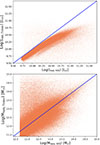 |
Fig. A.1. Upper panel: Comparison between the total optical luminosity provided by T21 and the value provided by Y05. The blue solid line indicates the one-to-one relation. Bottom panel: Comparison between the halo mass proxy provided by T21 and the value provided by Y05 based on the respective Ltot. The blue solid line indicates the one-to-one relation. |
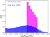 |
Fig. A.2. Distribution of the halo masses of T21 group catalog in the 1013.5 − 1014 M⊙ halo mass bin (magenta histogram) and of the matched groups in the Y05 (blue histogram). |
The greater scatter in mass proxy relations compared to Lopt (0.68 vs. 0.17 dex) indicates that the Lopt-to-halo mass calibration may also contribute. Y05 employs a single power-law for this conversion, while T21 applies distinct calibrations for blue and red galaxy groups (Alpaslan & Tinker 2020). Although weak lensing studies suggest a possible dependence on galaxy color (e.g., Mandelbaum et al. 2016), this trend is absent in local and high-redshift samples, where Lopt and halo mass derived from X-ray data show a consistent single power-law relation across galaxy properties (Erfanianfar et al. 2019, 2014).
In Fig. A.2, we observe that T21’s 1013.5 − 1014Mhalo mass bin (used in Fig. 15, left panel) spans a broader mass range under the Y05 proxy. The Y05 algorithm’s effectiveness in estimating halo mass and identifying central/member galaxies is supported by studies such as Marini et al. (2025), suggesting that T21 calibration may admit significant low-mass contamination across mass bins, potentially lowering mean X-ray flux in stacks by including low-luminosity, low-mass objects. A complete comparison would require incorporating the T21 algorithm into the mock dataset, as done for R11, Y05, and T17 in Marini et al. (2025). In conclusion, our analysis highlights that stacked X-ray results are highly sensitive to halo mass proxy systematics and selection biases in the prior catalog.
All Tables
All Figures
|
Fig. 1. Upper panel: completeness of the optical group catalogs based on the Magneticum mock galaxy catalog per bin of M200, FoF best proxy for R11 (red lines), T17 (orange lines), and Y05 (magenta lines) as obtained in Marini et al. (2024). The black line indicates the completeness of the X-ray selected sample extracted from the eROSITA mock observation with the eSASS detection algorithm as a function of the input M200 of Magneticum, as the X-ray selection algorithm gives no other mass proxy. Bottom panel: contamination of the optical group catalogs based on the Magneticum mock galaxy catalog per bin of original M200 of Magneticum for R11 (red lines), T17 (orange lines), and Y05 (magenta lines) as obtained in Marini et al. (2024). The black line indicates the contamination observed in the eSASS X-ray selected sample. |
| In the text | |
|
Fig. 2. Comparison between the input halo mass M200 and the group mass proxy based on the total luminosity scaled through the scaling relation of Popesso et al. (2005) for the three optically selected galaxy group samples: R11 (left panel), T17 (central panel) and Y05 (right panel. The solid line indicates the 1:1 relation. The green symbols indicate in all panels the mean M200 obtained in bins of 0.3 dex width of Mlum, whilst the error bars indicate the dispersion. The bottom panel shows the residuals Δ = log(Mlum)−log(M200) of the individual points and the mean values (green symbols) for the three group samples. |
| In the text | |
|
Fig. 3. Input halo mass M200 distribution corresponding to different bins of halo mass proxy Mlum. The left panel shows the results of the R11 group sample, the central panel the T17 group sample, and the right panel the results of the Y05 sample. The color code is indicated in the left panel. |
| In the text | |
|
Fig. 4. Predicted Magneticum X-ray surface brightness profiles per bin of halo mass. The profiles are obtained by convolving the PHOX projected profiles with the eROSITA PSF. The blue-shaded regions indicate the total X-ray emission within 1σ of the mean. The magenta blue-shaded regions indicate the AGN contribution, while the gray-shaded regions indicate XRB emission. The green-shaded region indicates the IGrM emission. |
| In the text | |
|
Fig. 5. Difference in ΔRA and ΔDec, estimated in kiloparsec, between the center of the eSASS detected extended emission and the center of the input halo. |
| In the text | |
|
Fig. 6. Difference in ΔRA and ΔDec, estimated in kiloparsec, between the center of the detected optical group and the center of the input halo (left panel), the coordinates of the eSASS X-ray detection and the center of the input halo (central panel), and the center of the detected optical group and of the eSASS X-ray detection. |
| In the text | |
|
Fig. 7. Difference in ΔRA and ΔDec, estimated in kiloparsec, between the center of the detected optical group and the center of the input halo (left panel), the coordinates of the eSASS X-ray detection and the center of the input halo (central panel), and the center of the detected optical group and of the eSASS X-ray detection. |
| In the text | |
|
Fig. 8. Comparison of the average projected PHOX profiles convolved with the eROSITA PSF and centered on the input halo center (blue points), the center coordinates of the R11 mock optically selected group sample (magenta symbols), and the X-ray center (orange triangle). The shaded region indicates the overlapping 1σ region. |
| In the text | |
|
Fig. 9. Distribution of the mass-weighted metallicity of the Magneticum halos estimated within r500 in different halo mass bins. The histograms are color coded as described in the figure according to the halo mass bin. |
| In the text | |
|
Fig. 10. Upper panels: relation between the input mass-weighted gas temperature derived within r500 for the Magneticum halos and the temperature derived from the optical halo mass proxy through the scaling relation of Lovisari et al. (2015) for each prior catalog: R11 (left panel), T17 (central panel), and Y05 (right panel). Each panel also shows the residuals in dex as a function of the gas temperature proxy. Bottom panels: expected temperature–emissivity relation, at fixed metallicity (0.3 Z⊙), estimated at the input mass-weighted gas temperature derived within r500 for the Magneticum halos and the X-ray emissivity (red curve in each panel). The green points indicate the emissivity corresponding to the temperature proxy obtained from the optical halo mass proxy of the different optically selected group samples (R11 left panel, T17 central panel, and Y05 right panel) and estimated for the same metallicity. |
| In the text | |
|
Fig. 11. Comparison in different halo mass bins between the PHOX input IGrM profiles convolved with the eROSITA PSF and averaged in input halo mass bins (green shaded region), with profiles averaged in halo mass proxy bins (colored symbols). The green-shaded region indicates the 1σ error. The colored points show the mean PHOX profiles obtained from the different prior catalogs (yellow for R11, orange for T17, and gold for Y05). The error bars indicate the 1σ uncertainty. |
| In the text | |
|
Fig. 12. Comparison in different halo mass bins between the PHOX input IGrM profiles convolved with the eROSITA PSF and the results of the stacking procedure on the mock observations. The PHOX profiles are averaged in bins of input halo mass, while the stacked profiles are obtained in bins of halo mass proxy of the related prior catalog (blue for R11, violet for T17, and pink for Y05). |
| In the text | |
|
Fig. 13. Comparison in different halo mass bins between the electron density profiles predicted by Magneticum (light pink points and solid curves) and the best-fit profiles obtained from the stacked X-ray surface brightness profiles of Fig. 12 of the three optical group catalogs of R11 (blue curve), Y05 (magenta curve) and T17 (purple curve). |
| In the text | |
|
Fig. 14. Comparison in different halo mass bins between the PHOX input IGrM profiles convolved with the eROSITA PSF (green-shaded region) and the observed stacked profiles of Popesso et al. (2025, blue-shaded region). The latter profiles were obtained by following the same stacking procedure used here and with the real R11 GAMA optically selected group catalog. The shaded regions indicate the 1σ uncertainty. |
| In the text | |
|
Fig. 15. Comparison in different halo mass bins between the PHOX IGrM input profiles convolved with the eROSITA PSF and the observed stacked profiles of Zhang et al. (2024, magenta-shaded region). The latter profiles were obtained by following the stacking procedure outlined in Zhang et al. (2024) and with the real Tinker (2021) optically selected group catalog in the SDSS area. The shaded regions indicate the 1σ uncertainty. |
| In the text | |
|
Fig. 16. LX–mass relation in the 0.5 − 2.0 keV band based on the stacking analysis applied to the Magneticum-eROSITA mock observations and based on the R11, T17 and Y05 optically selected galaxy group catalog. The relations are color coded as outlined in the figure: orange for R11, magenta for T17, and red for Y05 prior catalogs, respectively. The black symbols indicate the mean relation of the input Magneticum halos, while the black solid line indicates the best-fit obtained by considering input X-ray luminosity and mass for halos with M500 > 1013.5 M⊙. The cyan solid line indicates the relation of Pratt et al. (2009). The green solid line shows the relation of Lovisari et al. (2015) and the blue line the one of Chiu et al. (2022) in the 0.5 − 2.0 keV band. |
| In the text | |
|
Fig. 17. fgas − M500 relation. The filled circles represent a compilation of literature data, color coded as a function of the sample reference as shown in the picture. The black points connected by a solid line represent the Magneticum prediction. The squares indicate the fgas derived from the stacked X-ray surface brightness profiles. This is obtained by integrating the best-fit electron density model of Fig. 13. The dashed yellow and green curves represent the best-fit of Pratt et al. (2009) and Eckert et al. (2016), respectively. The dashed line indicates the value of the cosmic baryon fraction according to the WMAP cosmology implemented in Magneticum. |
| In the text | |
|
Fig. A.1. Upper panel: Comparison between the total optical luminosity provided by T21 and the value provided by Y05. The blue solid line indicates the one-to-one relation. Bottom panel: Comparison between the halo mass proxy provided by T21 and the value provided by Y05 based on the respective Ltot. The blue solid line indicates the one-to-one relation. |
| In the text | |
|
Fig. A.2. Distribution of the halo masses of T21 group catalog in the 1013.5 − 1014 M⊙ halo mass bin (magenta histogram) and of the matched groups in the Y05 (blue histogram). |
| In the text | |
Current usage metrics show cumulative count of Article Views (full-text article views including HTML views, PDF and ePub downloads, according to the available data) and Abstracts Views on Vision4Press platform.
Data correspond to usage on the plateform after 2015. The current usage metrics is available 48-96 hours after online publication and is updated daily on week days.
Initial download of the metrics may take a while.