| Issue |
A&A
Volume 704, December 2025
|
|
|---|---|---|
| Article Number | A146 | |
| Number of page(s) | 13 | |
| Section | Extragalactic astronomy | |
| DOI | https://doi.org/10.1051/0004-6361/202557189 | |
| Published online | 09 December 2025 | |
Delving into the depths of NGC 3783 with XRISM
III. Birth of an ultrafast outflow during a soft flare
1
SRON Space Research Organisation Netherlands, Niels Bohrweg 4, 2333 CA Leiden, The Netherlands
2
Leiden Observatory, Leiden University, PO Box 9513 2300 RA, Leiden, The Netherlands
3
RIKEN High Energy Astrophysics Laboratory, 2-1 Hirosawa, Wako, Saitama 351-0198, Japan
4
Department of Physics, Tokyo University of Science, 1-3 Kagurazaka, Shinjuku-ku, Tokyo 162-8601, Japan
5
Department of Physics and Astronomy, James Madison University, Harrisonburg, VA 22807, USA
6
Lawrence Livermore National Laboratory, Livermore, CA 94550, USA
7
University of Maryland College Park, Department of Astronomy, College Park, MD 20742, USA
8
NASA Goddard Space Flight Center (GSFC), Greenbelt, MD 20771, USA
9
Center for Research and Exploration in Space Science and Technology, NASA GSFC (CRESST II), Greenbelt, MD 20771, USA
10
Department of Physics, Technion, Haifa 32000, Israel
11
MIT Kavli Institute for Astrophysics and Space Research, Massachusetts Institute of Technology, Cambridge, MA 02139, USA
12
ESA European Space Astronomy Centre (ESAC), Camino Bajo del Castillo s/n, 28692 Villanueva de la Cañada, Madrid, Spain
13
ESA European Space Research and Technology Centre (ESTEC), Keplerlaan 1, 2201 AZ Noordwijk, The Netherlands
14
Space Telescope Science Institute, 3700 San Martin Drive, Baltimore, MD 21218, USA
15
Science Research Education Unit, University of Teacher Education Fukuoka, Munakata, Fukuoka 811-4192, Japan
16
Institute of Space and Astronautical Science (ISAS), Japan Aerospace Exploration Agency (JAXA), Kanagawa 252-5210, Japan
17
INAF – Osservatorio Astrofisico di Arcetri, Largo Enrico Fermi 5, I-50125 Florence, Italy
18
Graduate School of Science and Engineering, Kagoshima University, Kagoshima 890-8580, Japan
19
Astronomical Institute, Tohoku University, 6-3 Aramakiazaaoba, Aoba-ku, Sendai, Miyagi 980-8578, Japan
20
Department of Astronomy, University of Michigan, 1085 South University Avenue, Ann Arbor, MI 48109-1107, USA
⋆ Corresponding author: This email address is being protected from spambots. You need JavaScript enabled to view it.
Received:
10
September
2025
Accepted:
7
October
2025
Abstract
The 2024 X-ray/UV observation campaign of NGC 3783, led by XRISM, revealed the launch of an ultrafast outflow (UFO) with a radial velocity of 0.19c (57 000 km s−1). This event is synchronized with the sharp decay, within less than half a day, of a prominent soft X-ray/UV flare. Accounting for the look-elsewhere effect, the XRISM Resolve data alone indicate a low probability of 2 × 10⁻⁵ that this UFO detection is due to random chance. The UFO features narrow H-like and He-like Fe lines with a velocity dispersion of ∼1000 km s−1, suggesting that it originates from a dense clump. Beyond this primary detection, there are hints of weaker outflow signatures throughout the rise and fall phases of the soft flare. Their velocities increase from 0.05c to 0.3c over approximately three days, and they may be associated with a larger stream in which the clump is embedded. The radiation pressure is insufficient to drive the acceleration of this rapidly evolving outflow. The observed evolution of the outflow kinematics instead closely resembles that of solar coronal mass ejections, implying magnetic driving and, conceivably, reconnection near the accretion disk as the likely mechanisms behind both the UFO launch and the associated soft flare.
Key words: techniques: spectroscopic / galaxies: active / galaxies: Seyfert / X-rays: galaxies / X-rays: individuals: NGC 3783
© The Authors 2025
 Open Access article, published by EDP Sciences, under the terms of the Creative Commons Attribution License (https://creativecommons.org/licenses/by/4.0), which permits unrestricted use, distribution, and reproduction in any medium, provided the original work is properly cited.
This article is published in open access under the Subscribe to Open model. This email address is being protected from spambots. You need JavaScript enabled to view it. to support open access publication.
1. Introduction
Powerful, highly ionized winds with velocities of 0.1–0.3 times the speed of light and substantial column densities (NH ∼ 1023 cm−2) have been detected in the X-ray and UV spectra of luminous active galactic nuclei (AGNs; Pounds et al. 2003; Reeves et al. 2003; Tombesi et al. 2010; King & Pounds 2015; Nardini et al. 2015; Xrism Collaboration 2025). These so-called ultrafast outflows (UFOs) are primarily identified as highly blueshifted absorption lines in the X-ray spectra of quasars, and some studies indicate their presence in Seyfert galaxies as well (Pounds & Vaughan 2011; Tombesi et al. 2013). With kinetic energies reaching up to 1046 erg s−1, UFOs may be the drivers of AGN feedback, a process in which the central supermassive black hole transfers energy to its host galaxy on a large scale. Research suggests that outflows with mechanical energies exceeding 0.5–5% of the bolometric luminosity have the potential to expel gas and dust from the host galaxy, thereby suppressing star formation and explaining the observed M − σ relation (Hopkins & Elvis 2010; Fabian 2012; King & Pounds 2015). To better understand this feedback mechanism, it is crucial to observationally constrain the momentum and energy of UFOs and link these to larger-scale molecular outflows on kiloparsec scales.
Despite the increasing number of detections of X-ray UFOs, their geometry and formation mechanisms remain poorly understood. Plausible launching mechanisms include thermal driving (Begelman et al. 1983; Balsara & Krolik 1993; Chelouche & Netzer 2005), radiation driving (Ohsuga et al. 2009; Hagino et al. 2015; Ishibashi et al. 2018), magnetic driving (Fukumura et al. 2010, 2017), or a combination thereof. In many sub-Eddington sources with UFOs, the opacity is insufficient for radiative acceleration due to the high ionization state of the outflowing material. Magnetohydrodynamic (MHD) winds there offer a natural explanation for the high velocities of highly ionized material that does not involve line driving. An ultimate, comprehensive understanding of UFO launches and acceleration necessitates a systematic study of their properties (ionization, velocity, and energetics) in relation to fundamental AGN properties like luminosity, accretion rate, and black hole mass (Tombesi et al. 2012). High-resolution X-ray spectroscopy surveys of a broad sample of UFOs are essential for such an analysis.
Before such a comprehensive sample can be assembled, it is essential to determine other properties of UFOs. The equivalent widths and velocities of UFOs vary significantly on timescales down to hours. These variations can arise from the response of the wind to luminosity changes, or be intrinsic to the launching mechanism itself. The most useful observation would be of a newly formed UFO following an intrinsic change in the accretion structure. Utilizing XMM-Newton European Photon Imaging Camera (EPIC) data, Gallo et al. (2019) presented an intriguing case in Markarian 335, where a potential UFO with a velocity of 0.12c appeared after a flare event triggered by a structural change in the corona. The flare increased the radiation pressure by a factor of 5, which is potentially sufficient to launch the outflow. However, the limited spectral resolution with the CCD instruments and the transient nature of such events have generally hampered high-confidence UFO detections in this and the many other attempts made so far.
High-resolution X-ray spectroscopy provided by Resolve (Ishisaki et al. 2025; Kelley 2025) on board XRISM (Tashiro et al. 2025) represents a significant advance for studying UFOs. The micro-calorimeter can fully resolve Fe K-shell transitions in the energy band of interest, revealing the velocity and ionization structures of the outflows. Furthermore, time-resolved spectroscopy will allow the characterization of how UFOs respond to variations in the primary emission components of the AGN. Recent observations of the persistent UFO in PDS 456 revealed an absorption line profile with multiple narrow components, indicating clumpiness within a spherically outflowing wind (Xrism Collaboration 2025). In addition, a potential detection of time-varying UFOs in NGC 4151 has been reported by Xiang et al. (2025) using the Resolve data.
In this work we explore the presence of UFOs in NGC 3783 by utilizing a recent observation campaign involving XRISM. NGC 3783 is a Seyfert 1 galaxy that hosts an AGN powered by a black hole of mass 2.8 × 10⁷ M⊙ (Bentz et al. 2021) and an Eddington accretion rate of 0.07 (Summons et al. 2007). This AGN is well known for its prominent, semi-stable warm absorber outflows, characterized by narrow absorption lines with column densities of up to 1022 cm−2 and outflow velocities typically in the range 500 − 1500 km s−1 (Kaspi et al. 2001, 2002; Behar et al. 2003; Mehdipour et al. 2017; Mao et al. 2019; Gu et al. 2023). Obscuring outflows with higher column densities (up to 1023 cm−2) and faster velocities (around 2000 km s−1) have also occasionally been detected. The search for even faster outflows has led to mixed conclusions (Igo et al. 2020), as X-ray instruments prior to Resolve lacked the energy resolution and sensitivity to reliably detect absorption lines above 7 keV, especially those that vary on timescales shorter than a day.
This paper is arranged as follows. In Sect. 2 we describe the 2024 observational campaign and the search for UFOs. The properties of the possible outflows are discussed in Sect. 3 and summarized in Sect. 4. Throughout the paper, the errors are given at a 68% confidence level.
2. Data analysis and results
2.1. 2024 campaign
A 10-day observing campaign targeting NGC 3783 was carried out in late July 2024, led by XRISM, the new JAXA/NASA/ESA X-ray mission launched in September 2023. XRISM carries two primary instruments: the Resolve X-ray microcalorimeter spectrometer, offering an unprecedented energy resolution of 4.5 eV at 6 keV, and Xtend (Noda et al. 2025), an X-ray CCD imager that, while having lower energy resolution, provides better photon-collecting efficiency. Additional instruments participating in the coordinated campaign include the Reflection Grating Spectrometer (RGS), EPIC MOS and pn on board XMM-Newton, the High Energy Transmission Grating Spectrometer (HETGS) on Chandra, as well as NuSTAR, Swift, NICER, and the Cosmic Origins Spectrograph (COS) on board the Hubble Space Telescope. In this study, we mainly utilized data from XRISM, XMM-Newton, and NuSTAR.
Data reduction was performed using standard pipelines and procedures, in accordance with the cross-calibration paper (XRISM Collaboration 2025, Paper II) for this campaign. Details are not included here. The above paper also provides effective area correction factors for cross-calibration between XRISM, XMM-Newton, and NuSTAR, which have been applied in the current analysis.
Apart from Paper II of the series addressing cross-calibration issues from the 2024 observational campaign, the emission and absorption features of the time-averaged Resolve spectrum were reported in Paper I (Mehdipour et al. 2025). That work provided a detailed characterization of the quasi-steady, highly ionized outflows in NGC 3783. A total of six outflow components were resolved, including five typical warm absorbers with velocities ranging from 500 to 1200 km s−1, while the sixth component features a broad absorption dip with an outflowing velocity of 14 300 km s−1 (0.05c). Building on these existing results, this paper performs a search for time-variable, fast outflows using time-resolved spectra.
2.2. Soft X-ray flare
The Xtend light curves in the 0.3 − 0.6 keV and 3.0 − 6.0 keV energy bands were extracted to track changes in the soft and hard X-ray continua. These energy bands are selected to avoid known major emission and absorption features, such as the Fe unresolved transition array, Fe L-shell transitions, and the neutral Fe Kα line. The X-ray light curves shown in Fig. 1 display a series of significant variability patterns during this campaign. Over the ten days, the X-ray flux increases by about 60% in both the soft and hard X-ray bands, with multiple flares recurring on shorter timescales of around 150 ks (∼1.7 days). Among these variations, the period between 1.5 × 10⁵ s and 4 × 10⁵ s clearly needs particular attention. The hard X-ray intensity rises at t = 2 × 10⁵ s, synchronized with a nearly simultaneous increase in the soft X-ray band. While the hard X-rays peak at 2.6 × 10⁵ s and begin to decline, the soft X-rays continue to increase, peaking approximately 4 × 10⁴ s later. With the signature feature being a peak in soft X-rays, we refer to it as the “soft flare” hereafter. A secondary soft flare-like event appears toward the end of the campaign; however, since the second peak is only partially covered by the campaign, our analysis will focus on the primary soft flare.
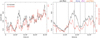 |
Fig. 1. XRISM Xtend light curves from the NGC 3783 campaign. Left: soft- and hard-band light curves, shown in black and red, respectively. The light curve has been binned to multiples of the XRISM orbit (5747 s), and in this paper we count time since the start of the XRISM observation. Right: X-ray variability surrounding the main soft flare at t ∼ 2.8 × 10⁵ s. |
To investigate the spectral variation in the soft flare, we divided the event into five periods as illustrated in Fig. 1 and Table 1. The net Resolve exposure time is approximately 25 ks for the rise, decay, and after-flare phases, 35 ks in the post-flare phase, and about 50 ks in the pre-flare phase.
Results from fitting the outflows.
Figure 2 displays the evolution of the hardness ratio during the soft flare event. The pre-flare phase begins with the hardest spectrum observed throughout the campaign, corresponding to the lowest overall luminosity. During the rise phase, the source transitions to a high state while exhibiting the softest spectrum recorded during the campaign. Throughout the decay and post-flare phases, the source bounced between harder and softer states before gradually relaxing to a stable hardness ratio in the post-flare phase. This flare event clearly exhibits the largest dynamical range in the hardness ratio, a striking contrast to the relatively stable level observed in the rest of the campaign.
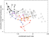 |
Fig. 2. Hardness ratio, defined by the count rates in the 3.0 − 6.0 keV and 0.3 − 0.6 keV bands, plotted against their combined count rate. Each data point represents a single XRISM orbit (5747 s). The data are color-coded by flare phase: pre-flare (black), rise (red), decay (blue), after-flare (magenta), and post-flare (orange). Gray points indicate observations outside the main soft flare. |
2.3. Outflow associated with the soft flare event
The Resolve spectrum during the soft flare period, from t = 1.3 × 10⁵ s to 4.3 × 10⁵ s, is analyzed based on the phases as defined in Fig. 1 and Table 1.
2.3.1. General spectral components applied to all phases
To search for spectral features associated with the soft flare, we modeled the Resolve spectrum in the 4.0 − 10.0 keV band based on the following components. The observed continuum was modeled in the same way as Paper I. A power-law component fits the primary continuum, with the photon index Γ obtained to be 1.79 ± 0.01. To account for potential soft X-ray excess, we included a warm Comptonization component, comt. Although the contribution of comt to the Resolve band is minor, ≈2%, it remains essential as a spectral energy distribution (SED) component for photoionization calculations. Since the comt parameters cannot be constrained with Resolve data, we fixed them to those of the 2001 unobscured model from Mehdipour et al. (2017). The power-law and comt components together form the SED used for photoionization calculations. In our time-resolved analysis, we allowed the normalization of both components and the photon index of the power-law component to vary freely.
Our model includes relevant narrow emission line components: Fe Kα, Fe Kβ, Ni Kα, Fe Lyα, and Fe Lyβ. These components are incorporated using Gaussian lines, following Paper I, including the line widths. We also considered the broad emission component, including the nonrelativistic component from the broad line region, as well as a relativistic component from the inner accretion disk. The broad line component is handled with a broad Gaussian and the relativistic component is accounted for with the Fe Kα convolved with the spei relativistic line profile component. These components are added in the same way as Paper I and Li et al., in prep.
The low-velocity ionized absorbers are modeled with the pion components (Mehdipour et al. 2016; Miller et al. 2015), in the same way as Paper I and Zhao et al., in prep. These components are found to be quasi-stable (Gu et al. 2023), and our analysis is not sensitive to minor variability within these warm absorbers. The pion components are fed with the year 2001 unobscured SED from Mehdipour et al. (2017), which is consistent with the intrinsic UV and X-ray continuum of our observation. The column density, ionization parameters, and kinetic properties of these components are fixed to the values reported in Paper I, which agrees with the full absorption measurement analysis in Zhao et al., in prep. The very high-velocity component X from Paper I, with an outflow velocity of about 0.05c, is not included as a general component in the baseline model, as it already qualifies as a UFO candidate. As shown later in Sect. 2.3.4, the component X likely exhibits significant variability.
As shown in Fig. 3, this model fits the time-average spectrum well during the entire soft flare period. It is established as our baseline, defining the starting point for the subsequent analysis.
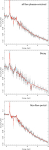 |
Fig. 3. Time evolution of the NGC 3783 Resolve spectra. Top: average spectrum over all flare phases. Middle: spectrum during the decay phase only. Bottom: average spectrum combining all periods outside the soft flare, shown for comparison. The dip at ∼8.4 keV is unique to the decay phase. The light blue curve in the middle panel shows the best-fit model excluding both the UFO and the 3700 km s−1 components. |
2.3.2. Possible detection of an ultrafast outflow
The most striking feature, as shown in Fig. 3, is an absorption dip centered at 8.4 keV during the decay phase. To characterize this feature, we incorporated a pion component on the baseline model. The power-law and comt components serve as the input SED, while the ionization parameter, column density, bulk velocity, and velocity dispersion are allowed to vary for the pion component. The warm absorbers and emission line components in the baseline model remain fixed at their time-averaged best-fit values, since their potential variability did not affect the observed dip. The results from the spectral analysis are summarized in Table 1.
Modeling the dip at 8.4 keV using a Gaussian absorption line reveals a C-stat improvement of 17. Employing the pion model yields a slightly enhanced ΔC of 20. This further improvement is probably caused by the fact that pion tends to include both H- and He-like Fe lines, accounting for the 8.4 keV dip as well as a secondary absorption feature near 8 keV. The best-fit ionization parameter (log ξ), column density, outflow velocity, and velocity dispersion are 3.2 ± 0.2, 1.1 ± 0.4 × 1023 cm−2, 56 780 ± 450 km s−1, and 1170 ± 350 km s−1. The outflow velocity indicates a UFO speed of 0.19c (∼57 000 km s−1).
The instrumental background of Resolve cannot explain the 8.4 keV dip. No instrumental features overlap with this energy, and the energies of the nearest background lines, including Cu Kα at 8.03 and 8.05 keV and Au Lα at 9.71 and 9.63 keV, are too different to explain the feature.
To improve confidence in our results, we cross-checked the detection with data from other instruments. The decay phase is well covered by Xtend, XMM-Newton, and NuSTAR. For these instruments, we conducted data reduction following the procedure described in the cross-calibration paper (XRISM Collaboration 2025). As shown in Fig. 4, the spectra from Xtend, NuSTAR, and XMM-Newton pn were modeled using the same baseline model as Resolve, while allowing the normalization and photon index of the power-law component to vary as to address cross-calibration uncertainties (XRISM Collaboration 2025). In the same plot, we also show the model incorporating the best-fit pion component from Resolve. The parameters of the pion component are fixed to the Resolve values. While the lower spectral resolution of Xtend, NuSTAR, and XMM-Newton pn prevents the narrow feature from being fully resolved, the comparisons demonstrate a statistical preference with the Resolve solution. The inclusion of the pion component results in improvement of C-stat of 4.7, 6.8, and 7.6, with respect to the baseline model, for Xtend, NuSTAR, and XMM-Newton pn. The combined improvement in C-stat across all four instruments, including Resolve, is 39.1.
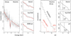 |
Fig. 4. Detailed look at the dip at 8.4 keV and the LEE. Left: Resolve, Xtend, NuSTAR, and XMM-Newton pn spectra from the decay phase. The red line shows the best-fit model to the Resolve data and including the UFO component, while the light blue line represents the model without it. Right: ΔC distribution from 1.3 × 10⁵ runs of the Monte Carlo simulation of the Resolve spectrum, and 1 × 10⁴ times for each of other three instruments (black histograms) and the observed ΔC distribution for the Resolve data (red histograms). Vertical lines mark the observed ΔC values for the other three instruments. |
The ΔC values reported above cannot be directly used to determine the confidence level of the detected feature. This limitation arises because, given the energy range explored during the analysis, the look-elsewhere effect (LEE) associated with detecting a random feature cannot be neglected. To address the LEE, we employed a Monte Carlo simulation approach. Following the methodologies outlined by Kosec et al. (2018) and Pinto et al. (2020), we first simulated a large set of spectra for each instrument, including 1.3 × 10⁵ times for Resolve, and 1 × 10⁴ for the others. The numbers of simulations correspond to the p-values associated with ΔC = 20 and 10, respectively.
The simulations were done with the baseline model for the decay phase and utilizing the actual exposure time. For each simulated spectrum, we scanned the 7.5 − 9.0 keV range with the pion model for the UFO and computed the ΔC relative to the baseline. Since no emission line was detected in the actual data, the scan did not include searches for emission features. The distribution of ΔC values from these simulations, representing the likelihood of random features, is shown in Fig. 4.
For Resolve, the occurrence N can be described as a function of ΔC by N = 10−0.23ΔC + 4.67. Integrating this function over the range of observed ΔC = 20 to infinity results in an expected frequency of ∼2 × 10⁻⁵. This frequency corresponds to an effective ΔC of 18. This suggests that the LEE would reduce the ΔC by 2 for Resolve. As shown in Fig. 4, the same exercise has been done for other instruments, and the effective ΔC of 3.8, 5.1,and 7.1 for Xtend, NuSTAR, and pn data, reducing 0.9, 1.7, and 0.5 from their original values. The combined effective ΔC is 34, leading to a random probability of 3 × 10⁻⁷ after accounting for the LEE.
2.3.3. Potential outflow at 3700 km s−1
Modeling the Resolve spectrum in the decay phase with the baseline model reveals another feature: the narrow Fe Kβ fluorescence line at approximately 7 keV appears to be absent. As shown in Fig. 5, this line is present during other phases of the flare, indicating that the narrow band at 7 keV varies on a timescale of less than or equal to 40 ks. To investigate whether this variability is due to intrinsic changes in the emission component, we allowed the relevant emission components to vary, including the narrow Fe Kβ line and the broad relativistic Fe line, which likely exhibits a cutoff around 7 keV (Li et al., in prep.). For this relativistic component, both the normalization and emissivity slope are set free. The new fit constrained the Fe Kβ/Fe Kα ratio to an upper limit of 0.035, significantly lower than the value with the baseline model of 0.12. This drastic change cannot be caused by the narrow line variation because there is no physical solution for such a line ratio change with a stable line center (Yamaguchi et al. 2014), and the observed 40 ks timescale variability is incompatible with a distant reflector origin of the narrow line.
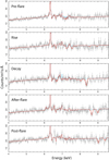 |
Fig. 5. Phase-resolved Resolve spectra during the soft flare. The best-fit models are shown in red. The light blue curves show the model that excludes both the UFO and the 3700 km s−1 component. |
The remaining possibility is that an absorption feature from an outflow overlaps in energy with the narrow Fe Kβ line. To address this, we incorporated two pion components into the baseline model; one for the known outflow at 0.19c and another for the absorption at Fe Kβ. The best-fit parameters for the new pion component are as follows: log ξ = 2.9 ± 0.1, column density = 5.9 ± 1.3 × 1022 cm−2, outflow velocity = 3720 ± 480 km s−1, and velocity dispersion = 1470 ± 530 km s−1. In fact, this additional component absorbs the continuum around 7 keV, causing the Fe Kβ line to appear as if it is missing, because the emission line happens to “fill in” the absorption dip in the continuum.
Including this component improves the C-statistic by 19. Taking into account the LEE, in the same way as for the UFO component (Sect. 2.3.2), yields a random probability of approximately 3 × 10⁻⁵. The outflow velocity associated with this component is significantly higher than that of the normal warm absorbers in NGC 3783, yet lower than the UFO components. Looking at past observations, another transient outflow component that also obscured the Fe Kβ line is the high-ionization component reported in Mehdipour et al. (2017) using XMM-Newton CCD data. This component had a velocity of about 2300 km s−1 and a column density of 1 − 2 × 1023 cm−2, identified during an obscuration event in 2016.
The 3700 km s−1 component appears to be transient, possibly related to the launch of the UFO at 0.19c (∼57 000 km s−1). As this paper focuses on the UFO component, the nature of 3700 km s−1 component will be discussed in a separate paper.
2.3.4. Search for outflows in other phases
A visual examination of Fig. 5 suggests the potential presence of further absorption features in the other phases of the flare. To systematically search for absorbers, we scanned the phase-resolved spectrum using a pion component added to the baseline model. In each iteration (n), the bulk velocity of the pion component was set to n × 1000 km s−1, while its column density, ionization parameter, and velocity dispersion were set as free parameters. The normalization and photon index of the power law, along with the normalization of the comt component, were also left free. Meanwhile, the warm absorbers and emission components remained fixed at their time-averaged values.
As shown in Fig. 6, the statistical significance of the pion component is plotted against the scanning velocity of n × 1000 km s−1. To evaluate the contribution of random variations, we present a comparison in Fig. 7 between the observed ΔC diagram and the expected distribution derived from Poisson data. To maximize statistical significance, we combined the rise, decay, after-, and post-flare phases in the comparison. The pre-flare phase was excluded due to its potential broad absorption features, which would have resulted in bins that are not fully independent. The comparison indicates that features detected with ΔC < 9 are likely due to Poisson noise. Peaks with ΔC ≥ 9 may have a higher likelihood of being real. Their actual significance will be evaluated considering the LEE, which will be detailed in Appendix A. We also attempted to enhance the detection of the potential outflow by combining the Resolve data with those from other instruments. The likelihood presented in Table 1 takes into account the best-fit and the LEE simulations from all instruments. It can be inferred that the CCD instruments show qualitative agreement with the presence of the pion component during all phases, though the overall improvement on the detection significance remains modest except for the decay phase.
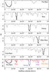 |
Fig. 6. Potential features identified with the pion scan on the Resolve data. The curves show the ΔC obtained in each step of the scan. The most prominent feature in each phase is highlighted with a thick line. In the bottom panel, all individual curves from the upper panels are combined and presented on a common ΔC scale for comparison. |
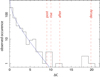 |
Fig. 7. LEE in the pion scan. The black histogram shows the combined ΔC distribution from the rise, decay, after, and post-flare phases. The blue line represents an exponential fit to this histogram, following a form similar to that described in Sect. 2.3.2. The dashed red lines mark the ΔC values of the most prominent features identified in these phases. |
The relatively large uncertainties in the column densities listed in Table 1 suggest a low confidence level for the fast outflow feature, except during the decay phase. However, we caution that the error on the hydrogen column density may not be an ideal indicator of significance, as it can be highly degenerate with the ionization parameter for a single absorption feature.
As detailed in Table 1, the pre-flare phase is characterized by a significant outflow with a velocity of 0.05c and a velocity dispersion of 4500 km s−1. These kinematic parameters show a good agreement with component X, which was identified in the time-averaged Resolve spectrum and reported in Paper I of the NGC 3783 series (Mehdipour et al. 2025).
To enable a direct comparison with component X, we fixed the ionization parameter (log ξ) of the pre-flare component at 4, aligning with the value assumed in Paper I. This yielded a best-fit column density of 1.1 × 1023 cm−2, which agrees with component X. This indicates that, when accounting for the potential degeneracy in the parameter space between the ionization parameter and the column density, the 0.05c component in the pre-flare is indeed consistent with the component X identified in the time-averaged spectrum.
In the post-flare phase, Fig. 5 reveals a potential extra narrow emission component at around 6.6 keV. This feature is well described by a narrow Gaussian with σ ∼ 200 km s−1, improving the C-stat by 18. Since it may form a P-Cygni profile with the adjacent Fe XXV absorption feature from the warm absorber, this emission could be associated with slow outflows.
Although the statistical uncertainties on the outflow velocity are less than 1000 km s−1 from the rise to the post-flare phases, the systematic uncertainties may be larger. Taking the decay spectrum as an example, the current best-fit solution associates the main absorption dip at ∼8.4 keV with Fe XXVI, with a secondary feature at ∼8 keV corresponding to Fe XXV. The overall outflow velocity is then approximately 0.19c. However, as shown in Fig. 6, the pion scan suggests an alternative possibility with an outflow velocity of 0.24c, where the main dip at ∼8.4 keV is instead caused by Fe XXV absorption. Although this alternative model has a ΔC value worse by 8 compared to the best-fit, it can be considered a source of systematic uncertainty on the outflow velocities.
In summary, we identify a potential outflow event during the strong soft flare in NGC 3783, with the most significant feature observed at v ≈ 0.19c during the decay phase. Furthermore, Resolve spectra suggest the potential presence of outflow signatures in other flare phases as well, exhibiting velocities that rise from 0.05c to 0.3c within a total time span of 3 × 10⁵ s.
3. Discussion
In this section we closely examine the observed physical properties of the potential outflow and explore the various processes that could potentially explain its observed kinematics.
3.1. Constraints on the ionization and column density
As shown in Fig. 8, the ionization parameter of the UFO exhibits an increase from 2.7 ± 0.1 during the pre-flare phase to 3.3 ± 0.1 during the rise phase, followed by a smooth decline back to 2.7 ± 0.1. Since the continuum luminosity in the 1 − 1000 Rydberg range approximately doubles from the pre- to rise phases and then decreases by a factor of 1.7 during the rise to post-flare transition, the observed change in ionization parameter broadly agrees with the flaring luminosity variation. This suggests that the upper limit on the temporal change in the product of density and squared distance (nR2) across the flare is approximately a factor of 2.
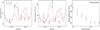 |
Fig. 8. Evolution of outflow parameters during the flare. Left: outflow parameter. Middle: column density. These two panels are overlaid with the soft-band (black) and hard-band (red) X-ray light curves. A horizontal dashed line in the middle panel indicates the average column density excluding the decay phase. Right: column density as a function of the covering factor for the decay phase. |
Figure 8 also shows that the observed column density remains relatively stable within the range 2 − 4 × 1022 cm−2, except possibly during the decay phase, where it is about 3 − 5 times higher than the average. This suggests that while the outflow is generally stable, a denser clump may enter the line of sight during the flare decay. These column densities are consistent with recent XRISM measurements of UFOs in PDS456 (Xrism Collaboration 2025), and higher than the column density of 3 × 1021 cm−2 found in PG 1211+143 with the Chandra grating (Danehkar et al. 2018). Considering relativistic effects as discussed in Luminari et al. (2020), the actual column densities are likely underestimated; applying their correction implies ∼2 × 1023 cm−2 during decay and around 4 × 1022 cm−2 otherwise.
A key systematic uncertainty in the column density measurement arises from the covering factor of the outflow component. In our analysis, we assumed full coverage of the X-ray source, but in principle, the outflow could be only partially covering the source. To investigate this, we refit the spectrum by manually varying the covering factor of the pion component. As shown in Fig. 8, the column density of the UFO increases from ∼1 × 1023 cm−2 to about 4 × 1023 cm−2, while the covering factor decreases from 1 to 0.4. The C-stat remains nearly unchanged across this range. A covering factor below 0.4 results in dips that are too shallow to reproduce the observed 8.4 keV feature. This suggests that the projected area of the outflow cannot be much smaller than the X-ray emitting region at this energy.
3.2. Constraints on the density and location
To better understand the physical properties of the outflow, we estimated the density and distance constraints based on geometrical considerations. Assuming that the cloud thickness (ΔR) equals its distance from the black hole (R), the column density (NH) and the minimum density (nlow) are related by
 (1)
(1)
Combining this with the definition of the ionization parameter yields
 (2)
(2)
where ξ is the ionization parameter and L is the ionizing luminosity. The maximum distance Rupp follows as
 (3)
(3)
Using the observed parameters, the outflow density exceeds 1 × 105 cm−3 during the decay phase and averages around 1 × 104 cm−3 in other phases. Due to the loose lower limit on density, the distance constraint remains broad, with Rupp ∼ 1 × 10⁵Rg.
A second constraint can be obtained by assuming the outflow is just capable of escaping the gravitational potential of the supermassive black hole. The boundary between escaping and failed outflow occurs when the outflow velocity equals  , where G is the gravitational constant, and MBH = 2.8 × 10⁷ M⊙ (Bentz et al. 2021). By substituting the escape velocity-based distance into the ionization parameter definition, the density can be expressed as
 (4)
(4)
where v is the outflow velocity that can be approximated by the radial velocity listed in Table 1 for an order-of-magnitude estimate. As shown in Fig. 9, nesc serves as an upper limit, which in turn provides a lower limit on the distance Resc. During the decay phase, the outflow density is constrained to be below 1012 cm−3, while the corresponding distance is likely above 50 Rg.
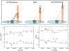 |
Fig. 9. Constraints on the density and distance of the outflow. Top: schematic illustrating a simple scenario: a clumpy outflow stream moving vertically from near the accretion disk, with the clump represented by the circle. Bottom: Density (left) and distance (right) constraints derived from the geometrical limits (nlow and Rupp) and escape velocity (nesc and Resc). Stars mark the density and distance values assuming that a clumpy component, observed during the decay phase, was launched at the pre-flare onset. The dashed line shows the density and distance limits estimated from the duration of the 8.4 keV dip during the decay phase. |
While the above two approaches offer loose constraints on the density and location of the UFO, we next considered a more speculative scenario to obtain a tighter limit. The UFO is a stream − a broad and relatively diffuse outflow launched vertically from the accretion disk (Fukumura et al. 2010). As illustrated in Fig. 9, at each phase a portion of this stream passes through our line of sight within the 6.0 − 10.0 keV energy range. During the pre-flare, rise, after, and post-flare phases, we observe the stream itself, allowing us to track velocity changes over time. We speculate that a dense and discrete clump, which is embedded within and comoving with the stream (Takeuchi et al. 2013), enters our line of sight at the start of the decay phase and exits by its end. The decay phase thus offers a unique ∼40 ks window to directly study the properties of this clump.
Although this is a speculative model, it provides a reasonable explanation for the observed constant column density, which only increases during the decay phase (Fig. 8). An alternative idea is that the clump is always visible but only fully covers the hard X-ray line of sight during the decay phase, with partial covering at other times. While plausible, this alternative scenario would not change the main conclusions derived from our proposed stream model.
Based on the observed radial velocities listed in Table 1, and an inclination angle of 23° reported in GRAVITY Collaboration (2021), we can estimate the vertical velocity of the stream at each phase. Assuming that the main clump was launched at the start of the pre-flare phase and followed the stream velocity during its lift-up, its vertical displacement would reach approximately 120 Rg by the decay phase. This corresponds to a radial distance of roughly 130 Rg. Based on the observed luminosity and ionization parameter, the inferred density is approximately 1 × 1011 cm−3. This value is consistent with the constraints obtained above, nlow and nesc. It is also in agreement with densities reported in other UFO studies (Fukumura et al. 2018).
This geometrical model suggests a launch radius of approximately sin(23° ) × 130 = 50 Rg for the UFO. This location is noteworthy because, according to the standard thin disk model (Shakura & Sunyaev 1973), using the black hole mass of 2.8 × 10⁷ M⊙ (Bentz et al. 2021) and an Eddington accretion rate of 0.07 (Summons et al. 2007), the dynamical timescale of the disk at 50 Rg is estimated to be Tdyn ∼ 1 × 10⁵ s. Interestingly, this timescale closely matches with the observed duration of the soft X-ray flare (Fig. 1). At the same radius, the disk rotation timescale is 2πTdyn ∼ 6× 10⁵ s, suggesting that orbital motion likely has a limited impact on the outflow kinematics over the observed period.
Our geometrical scenario, as illustrated in Fig. 9, further suggests that the clump obscures and passes through the X-ray emission region within the decay phase, over a timescale of no more than 4 × 10⁴ s. This implies that the transverse travel distance is at least equal to the combined diameters of the clump and the X-ray corona at 8 keV. Assuming the clump fully covers the emission region during this phase, both the clump and the hard X-ray corona would have diameters of 12 Rg. If the covering factor is less than 1, the clump size would decrease while the corona size increases. As shown in Fig. 8, the minimal covering factor is about 0.4, corresponding to a clump diameter of 10 Rg and corona size of 16 Rg. Therefore, we considered 12 Rg to be the upper limit for the clump diameter.
Assuming that the outflow stream also has a thickness of 12 Rg, we derive a lower limit on the density of the clump of approximately 3 × 109 cm−3. This places the radial distance of the outflow during the decay phase at less than 1000 Rg (Fig. 9). These constraints are consistent with all the previous limits derived earlier. This estimate is based on the assumption of a spherical clump; if the clump itself is stream-like with a smaller thickness, the actual radial distance could be further smaller.
In summary, the observed properties can be adequately explained by a relativistic outflow originating at about 50 Rg from the innermost region of the disk. This is in broad agreement with the UFO detected in PDS 456 with XRISM (Xrism Collaboration 2025). The prominent feature during the decay phase can be attributed to a major clump within this flow, with a density of about 1 × 1011 cm−3.
3.3. Constraints on the velocity and acceleration
In Fig. 10 we show the evolution of the outflow velocity obtained from the Resolve data, along with the corresponding acceleration. The best-fit velocity increases from 0.05c to 0.3c over about 2 × 10⁵ s, with the acceleration peaking at roughly 0.6 km s−2 around the time of 2.8 × 10⁵ s.
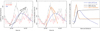 |
Fig. 10. Comparison of UFO and CME dynamics. Left: evolution of the UFO velocity (in black). Middle: evolution of the UFO acceleration (in orange). Both panels are overlaid with the XMM-Newton OM (blue), soft-band (gray), and hard-band (red) X-ray light curves. Right: schematic view of the early dynamic evolution of a typical CME event close to the Sun, adapted from Temmer (2016). We see that the UFO and CME patterns are similar to each other, with the acceleration phase aligning with the hard-band flare and the velocity correlating with the soft-band flare. |
Assuming that the outflow is launched at 50 Rg, the observed radial velocity of 0.05c at the pre-flare phase (Table 1) falls well below the escape velocity of 0.19c. This implies that the outflow in the pre-flare phase would not escape without significant acceleration. The acceleration that in fact occurs during the soft flare, however, propels the outflow to 130 Rg by the decay phase. At this point, its observed velocity of 0.19c (Table 1) now significantly exceeds the local escape velocity of 0.03c, confirming that the outflow has successfully escaped and is propagating away.
The direct acceleration on the wind gained by absorbing or scattering photons can be calculated as
![Mathematical equation: $$ \begin{aligned} a = \frac{\int F(E) [1 - T(E)] dE}{c f m_{\rm p} N_{\rm H}}, \end{aligned} $$](/articles/aa/full_html/2025/12/aa57189-25/aa57189-25-eq6.gif) (5)
(5)
where F(E) is the incoming energy flux, T(E) is the transmission, c is light speed, mp is the proton mass, NH is the column density, and f is the dimensionless factor related to the mass density via ρ = fnHmp, with nH being the hydrogen density. Using the observed flux, column density, and ionization parameter during the decay phase (Table 1), and assuming a wind density of 1 × 1011 cm−3, the resulting acceleration is on the order of 3 m s−2. This is two orders of magnitude smaller than the observed peak acceleration of 600 m s−2 shown in Fig. 10, indicating that radiation pressure alone is unlikely to drive the observed UFO acceleration.
The mass outflow rate can be estimated as
 (6)
(6)
where b is the covering factor of the outflow, v is the velocity at distance R. Taking a density of 1 × 1011 cm−3 and velocity of 0.2c at distance of 50 Rg, the mass loss rate is 7b solar mass per year. The actual value of b is unconstrained with current data, though it is likely small. The corresponding mechanical power is about 8b × 1045 erg s−1, which is roughly the Eddington luminosity scaled by b.
In fact, it is unlikely that the acceleration is fully continuous. A stable acceleration of 600 m s−2 would cause the central velocity of the absorption line to increase continuously by 24 000 km s−1 during the decay phase, far exceeding the observed velocity dispersion of only about 1200 km s−1 (Table 1). This discrepancy suggests that the acceleration is impulsive rather than steady. Instead of a smooth and persistent increase, the outflow probably accelerates in short and intense bursts, followed by periods of much weaker acceleration. Such impulsive behavior is characteristic of energetic solar phenomena (Vršnak et al. 2007 and references therein), which will be discussed in the following section.
3.4. Comparison with coronal mass ejection events
We further compare the evolution of UFO velocity and acceleration with the X-ray and optical/UV light curves in Fig. 10. The optical/UV light curve is derived from XMM-Newton Optical Monitor (OM) data, as outlined in Appendix B. We observe a 6.6% increase in the UV flux of NGC 3783 following the soft X-ray flare, with its temporal behavior consistent with a smooth burst model. Interestingly, the UFO velocity appears to correlate with the rise in UV flux, and the peak outflow acceleration coincides with the maximum in the 0.3 − 0.6 keV band. The hard X-ray light curve reaches its maximum before both the UV and soft X-ray light curves.
It has been proposed that some of the UFOs might originate from MHD acceleration (Fukumura et al. 2018). This scenario may resemble the physics of coronal mass ejections (CMEs), which are massive eruptions of plasma and magnetic fields from stellar coronae into space. CMEs are often observed alongside flares, current sheets, and plasma eruptions, likely driven by rapid magnetic reconnection (Di Matteo 1998; Patel et al. 2020). Statistical analyses of CMEs during their early near-Sun evolution (Zhang & Dere 2006; Temmer 2016) suggest a two-phase process: an initial slow rise lasting tens of minutes, followed by a rapid acceleration to reach maximum velocity. Comparing the temporal evolution of observed UFO and CMEs reveals potential similarities: the velocity appears to track emission in the longer wavelength (soft X-ray for CMEs and UV for the UFO), while the acceleration correlates better with emission at shorter wavelength (hard X-ray for CMEs and soft X-ray for the UFO).
To compare their characteristic outflow velocities, we utilized the Alfvén speed as a proxy,
 (7)
(7)
where B is the field strength, μ0 is permeability of free space, and ρ is the mass density. For CMEs, adopting B = 10 Gauss and ρ = 10−15 g cm−3 in the corona (Aschwanden 2005), the Alfvén speed is about 1000 km s−1. As for the UFO, assuming a magnetic field strength of 104 Gauss and mass density of 10−15 g cm−1 in the AGN corona (Merloni & Fabian 2001), the Alfvén speed becomes about 0.3c. This scaling shows a rough agreement with the observed outflow velocities in typical CMEs and the UFO in NGC 3783. The assumed field strength of 104 Gauss is consistent with the maximum expected value derived from the α-disk prescription (see Shakura & Sunyaev 1973, Eq. (2.19)).
Following, for example, Ohyama & Shibata (1997) and Tsuneta et al. (1997), the total energy release rate from a magnetic reconnection event can be described by
 (8)
(8)
where vinflow is the reconnection inflow speed, Lr is the characteristic scale of the reconnection region, EUFO is the kinetic energy of the UFO, and ER is the total radiative energy enhancement in the flare. The left side represents the energy input from reconnection, which is likely larger than the right side, as some energy may be channeled into other forms such as conductive flux.
Here we assumed that the reconnection region has a scale similar to the clump size of the UFO, Lr = 12Rg (see details in Sect. 3.2). Taking B = 104 Gauss and vinflow = 0.1vA (Di Matteo 1998), the total energy release rate through reconnection is approximately 2 × 1044 erg s−1. This is an order-of-magnitude estimate. Comparing this with the observed broad-band X-ray luminosity enhancement during the flare, which is roughly 2 × 1043 erg s−1, indicates that about 10% of the injected energy is radiated away in X-ray.
Furthermore, as discussed in Sect. 3.3, the kinetic power of the outflow is estimated as 8b × 1045 erg s−1, where b is the UFO covering factor. From Eq. (8), this implies a small covering factor of b ≤ 0.02. The small covering is physically plausible, considering the potential filamentary nature of the outflow suggested in Fig. 9.
As reported in, for example, Kontar et al. (2017), the velocity dispersions of the CME ejecta are on the order of ∼100 km s−1, which are much lower than their bulk velocities of ∼1000 km s−1. This suggests that a coherent magnetic structure driving the CME would suppress small-scale motions. Similarly, as shown in Table 1, the bulk flow represents the dominant form of kinetic energy in the UFO in NGC 3783.
Evidence of CME-like eruptions during soft X-ray flares has been observed in Galactic microquasars (Fender et al. 1999) and in Sgr A*. Although the origin of this correlation remains uncertain, theoretical and simulation studies suggest that rotating magnetic field lines inflate and reconnect above the disk, rapidly heating the corona during flares, while simultaneously expanding and launching plasma-loaded magnetic flux tubes that constitute the UFO (Yuan et al. 2009). Reconnection could involve poloidal fields (El Mellah et al. 2023), toroidal fields on the disk (Machida & Matsumoto 2003), or a combination of the two. A few MHD simulations have also explored the connection between such eruptions and various accretion disk configurations, including magnetically arrested disks (Narayan et al. 2003).
It is plausible that magnetic reconnection-triggered UFOs induce quasi-periodic X-ray flares (Ripperda et al. 2020). The periodicity of these flares is crucial for constraining the reconnection rate. While the X-ray light curve of NGC 3783, shown in Fig. 1, exhibits features resembling quasi-periodic variations, a comprehensive quantitative search for periodicity remains nontrivial and will be addressed in a subsequent study. The XRISM campaign on NGC 3783 offers a promising vision; to fully understand UFO launching and energy transport in the innermost regions of the accretion disk, it is still essential to collect more flare–UFO cases across different systems. Long-term monitoring and high-resolution spectroscopy with XRISM and upcoming missions such as NewAthena (Cruise et al. 2025; Peille et al. 2025) will be vital for advancing this research.
4. Summary
The ten-day spectroscopic campaign that observed NGC 3783, conducted with XRISM in combination with six other X-ray and UV observatories, offered an unprecedented opportunity for unexpected discoveries. The X-ray light curve shows multiple flares, including a major event characterized by initial hard X-ray peaks followed by a strong soft X-ray peak. During the decay of this soft flare, an absorption feature at 8.4 keV in the Resolve spectrum suggests the presence of a UFO with a radial velocity of 0.19c (∼57 000 km s−1). This outflow may not be an isolated event but rather part of a broader outburst that lasted approximately three days. A secondary outflow, with a velocity of about 3700 km s−1, was also detected coincident with the UFO. Based on the physics constraints derived from the Resolve data, it is plausible that magnetic fields within the accretion disk serve as the central engine driving the UFO launch in this low-L/LEdd AGN. This mechanism may also be linked to the observed soft flare.
Acknowledgments
SRON is supported financially by NWO, the Netherlands Organization for Scientific Research. KF acknowledges support from NASA grant 80NSSC23K1021. Part of this work was performed under the auspices of the U.S. Department of Energy by Lawrence Livermore National Laboratory under Contract DE-AC52-07NA27344. The material is based upon work supported by NASA under award number 80GSFC21M0002. EB acknowledges support from NASA grants 80NSSC20K0733, 80NSSC24K1148, and 80NSSC24K1774. M. Mehdipour acknowledges support from NASA grants 80NSSC23K0995 and 80NSSC25K7126. This work was supported by JSPS KAKENHI Grant Numbers JP21K13963, JP24K00672, JP24K00638, JP21K13958, JP24K17104, JP25H00660. AT and the present research are in part supported by the Kagoshima University postdoctoral research program (KU-DREAM). KF is grateful to Emeritus Professor of Kyoto University, Kazunari Shibata, for a fruitful discussion on magnetic reconnection. MS acknowledges support through the European Space Agency (ESA) Research Fellowship Programme in Space Science. M. Mizumoto acknowledges support from Yamada Science Foundation.
References
- Aschwanden, M. J. 2005, Physics of the Solar Corona. An Introduction with Problems and Solutions, 2nd edn. [Google Scholar]
- Balsara, D. S., & Krolik, J. H. 1993, ApJ, 402, 109 [NASA ADS] [CrossRef] [Google Scholar]
- Begelman, M. C., McKee, C. F., & Shields, G. A. 1983, ApJ, 271, 70 [CrossRef] [Google Scholar]
- Behar, E., Rasmussen, A. P., Blustin, A. J., et al. 2003, ApJ, 598, 232 [Google Scholar]
- Bentz, M. C., Williams, P. R., Street, R., et al. 2021, ApJ, 920, 112 [NASA ADS] [CrossRef] [Google Scholar]
- Chelouche, D., & Netzer, H. 2005, ApJ, 625, 95 [NASA ADS] [CrossRef] [Google Scholar]
- Cruise, M., Guainazzi, M., Aird, J., et al. 2025, Nat. Astron., 9, 36 [Google Scholar]
- Danehkar, A., Nowak, M. A., Lee, J. C., et al. 2018, ApJ, 853, 165 [NASA ADS] [CrossRef] [Google Scholar]
- Di Matteo, T. 1998, MNRAS, 299, L15 [NASA ADS] [CrossRef] [Google Scholar]
- El Mellah, I., Cerutti, B., & Crinquand, B. 2023, A&A, 677, A67 [NASA ADS] [CrossRef] [EDP Sciences] [Google Scholar]
- Fabian, A. C. 2012, ARA&A, 50, 455 [Google Scholar]
- Fender, R. P., Garrington, S. T., McKay, D. J., et al. 1999, MNRAS, 304, 865 [Google Scholar]
- Fukumura, K., Kazanas, D., Contopoulos, I., & Behar, E. 2010, ApJ, 715, 636 [NASA ADS] [CrossRef] [Google Scholar]
- Fukumura, K., Kazanas, D., Shrader, C., et al. 2017, Nat. Astron., 1, 0062 [NASA ADS] [CrossRef] [Google Scholar]
- Fukumura, K., Kazanas, D., Shrader, C., et al. 2018, ApJ, 864, L27 [NASA ADS] [CrossRef] [Google Scholar]
- Gallo, L. C., Gonzalez, A. G., Waddell, S. G. H., et al. 2019, MNRAS, 484, 4287 [Google Scholar]
- GRAVITY Collaboration (Amorim, A., et al.) 2021, A&A, 648, A117 [NASA ADS] [CrossRef] [EDP Sciences] [Google Scholar]
- Gu, L., Kaastra, J., Rogantini, D., et al. 2023, A&A, 679, A43 [NASA ADS] [CrossRef] [EDP Sciences] [Google Scholar]
- Hagino, K., Odaka, H., Done, C., et al. 2015, MNRAS, 446, 663 [NASA ADS] [CrossRef] [Google Scholar]
- Hopkins, P. F., & Elvis, M. 2010, MNRAS, 401, 7 [NASA ADS] [CrossRef] [Google Scholar]
- Igo, Z., Parker, M. L., Matzeu, G. A., et al. 2020, MNRAS, 493, 1088 [NASA ADS] [CrossRef] [Google Scholar]
- Ishibashi, W., Fabian, A. C., & Maiolino, R. 2018, MNRAS, 476, 512 [NASA ADS] [Google Scholar]
- Ishisaki, Y., Kelley, R. L., Awaki, H., et al. 2025, J. Astron. Telesc. Instrum. Syst., 11, 042023 [Google Scholar]
- Kaspi, S., Brandt, W. N., Netzer, H., et al. 2001, ApJ, 554, 216 [NASA ADS] [CrossRef] [Google Scholar]
- Kaspi, S., Brandt, W. N., George, I. M., et al. 2002, ApJ, 574, 643 [NASA ADS] [CrossRef] [Google Scholar]
- Kelley, R. L. 2025, JATIS, accepted [Google Scholar]
- King, A., & Pounds, K. 2015, ARA&A, 53, 115 [NASA ADS] [CrossRef] [Google Scholar]
- Kontar, E. P., Perez, J. E., Harra, L. K., et al. 2017, Phys. Rev. Lett., 118, 155101 [NASA ADS] [CrossRef] [Google Scholar]
- Kosec, P., Pinto, C., Fabian, A. C., & Walton, D. J. 2018, MNRAS, 473, 5680 [NASA ADS] [CrossRef] [Google Scholar]
- Luminari, A., Tombesi, F., Piconcelli, E., et al. 2020, A&A, 633, A55 [NASA ADS] [CrossRef] [EDP Sciences] [Google Scholar]
- Machida, M., & Matsumoto, R. 2003, ApJ, 585, 429 [NASA ADS] [CrossRef] [Google Scholar]
- Mao, J., Mehdipour, M., Kaastra, J. S., et al. 2019, A&A, 621, A99 [NASA ADS] [CrossRef] [EDP Sciences] [Google Scholar]
- Mehdipour, M., Kaastra, J. S., & Kallman, T. 2016, A&A, 596, A65 [NASA ADS] [CrossRef] [EDP Sciences] [Google Scholar]
- Mehdipour, M., Kaastra, J. S., Kriss, G. A., et al. 2017, A&A, 607, A28 [NASA ADS] [CrossRef] [EDP Sciences] [Google Scholar]
- Mehdipour, M., Kaastra, J. S., Eckart, M. E., et al. 2025, A&A, 699, A228 [NASA ADS] [CrossRef] [EDP Sciences] [Google Scholar]
- Merloni, A., & Fabian, A. C. 2001, MNRAS, 321, 549 [NASA ADS] [CrossRef] [Google Scholar]
- Miller, J. M., Kaastra, J. S., Miller, M. C., et al. 2015, Nature, 526, 542 [NASA ADS] [CrossRef] [Google Scholar]
- Narayan, R., Igumenshchev, I. V., & Abramowicz, M. A. 2003, PASJ, 55, L69 [NASA ADS] [Google Scholar]
- Nardini, E., Reeves, J. N., Gofford, J., et al. 2015, Science, 347, 860 [Google Scholar]
- Noda, H., Mori, K., Tomida, H., et al. 2025, PASJ, 77, S10 [Google Scholar]
- Ohsuga, K., Mineshige, S., Mori, M., & Kato, Y. 2009, PASJ, 61, L7 [NASA ADS] [Google Scholar]
- Ohyama, M., & Shibata, K. 1997, PASJ, 49, 249 [Google Scholar]
- Patel, R., Pant, V., Chandrashekhar, K., & Banerjee, D. 2020, A&A, 644, A158 [NASA ADS] [CrossRef] [EDP Sciences] [Google Scholar]
- Peille, P., Barret, D., Cucchetti, E., et al. 2025, Exp. Astron., 59, 18 [Google Scholar]
- Pinto, C., Walton, D. J., Kara, E., et al. 2020, MNRAS, 492, 4646 [Google Scholar]
- Pounds, K. A., Reeves, J. N., King, A. R., et al. 2003, MNRAS, 345, 705 [Google Scholar]
- Pounds, K. A., & Vaughan, S. 2011, MNRAS, 413, 1251 [Google Scholar]
- Reeves, J. N., O’Brien, P. T., & Ward, M. J. 2003, ApJ, 593, L65 [Google Scholar]
- Ripperda, B., Bacchini, F., & Philippov, A. A. 2020, ApJ, 900, 100 [NASA ADS] [CrossRef] [Google Scholar]
- Shakura, N. I., & Sunyaev, R. A. 1973, A&A, 24, 337 [NASA ADS] [Google Scholar]
- Summons, D. P., Arévalo, P., McHardy, I. M., Uttley, P., & Bhaskar, A. 2007, MNRAS, 378, 649 [NASA ADS] [CrossRef] [Google Scholar]
- Takeuchi, S., Ohsuga, K., & Mineshige, S. 2013, PASJ, 65, 88 [Google Scholar]
- Tashiro, M., Kelley, R., Watanabe, S., et al. 2025, PASJ [Google Scholar]
- Temmer, M. 2016, Astron. Nachr., 337, 1010 [NASA ADS] [CrossRef] [Google Scholar]
- Tombesi, F., Cappi, M., Reeves, J. N., & Braito, V. 2012, MNRAS, 422, L1 [Google Scholar]
- Tombesi, F., Cappi, M., Reeves, J. N., et al. 2010, A&A, 521, A57 [NASA ADS] [CrossRef] [EDP Sciences] [Google Scholar]
- Tombesi, F., Cappi, M., Reeves, J. N., et al. 2013, MNRAS, 430, 1102 [Google Scholar]
- Tsuneta, S., Masuda, S., Kosugi, T., & Sato, J. 1997, ApJ, 478, 787 [Google Scholar]
- Vršnak, B., Maričić, D., Stanger, A. L., et al. 2007, Sol. Phys., 241, 85 [Google Scholar]
- Xiang, X., Miller, J. M., Behar, E., et al. 2025, ApJ, 988, L54 [Google Scholar]
- XRISM Collaboration (Audard, M., et al.) 2025, A&A, 702, A147 [Google Scholar]
- Xrism Collaboration (Audard, M., et al.) 2025, Nature, 641, 1132 [Google Scholar]
- Yamaguchi, H., Eriksen, K. A., Badenes, C., et al. 2014, ApJ, 780, 136 [Google Scholar]
- Yuan, F., Lin, J., Wu, K., & Ho, L. C. 2009, MNRAS, 395, 2183 [NASA ADS] [CrossRef] [Google Scholar]
- Zhang, J., & Dere, K. P. 2006, ApJ, 649, 1100 [NASA ADS] [CrossRef] [Google Scholar]
Appendix A: Look elsewhere effect in the phase-resolved spectra
In this appendix we present additional information that addresses the LEE in the phase-resolved spectra of the soft flare. The approach has been detailed in Sect. 2.3.2 for the potential detection of UFOs in the decay phase. Here, we applied the same method to the other phases and provide the corresponding significance.
For each phase, we simulated a set of 1.3 × 10⁵ spectra for Resolve, and 1 × 10⁴ for other instruments, based on the baseline model. For each simulated spectrum, we scanned the 7.0 − 9.0 keV range with the pion model for the UFO and computed the ΔC relative to the baseline. In Fig. A.1 we plot the observed and simulated ΔC diagram for Resolve. The original ΔC improvements of 12, 10, 12, and 9 for the pre-, rise, after-, and post- flare phases, become 11.5, 9.5, 11.4, 8.3 after correcting for the LEE. The effect of LEE is reflected in the significance shown in Table 1.
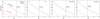 |
Fig. A.1. Histogram of ΔC distributions for Resolve. The black histogram shows the results from 1.3 × 10⁵ Monte Carlo simulations per phase, and the observed distribution is shown in red. Vertical lines mark the positions of the best-fit features. |
For all phases, the data from the CCD instruments agree with the best-fit model shown in Table 1. In the decay phase, the collection of CCD data boosts the significance of the UFO feature. In the other phases, since the possible features are much weaker, the LEE effect becomes more dominant; therefore, the relative boost from the CCD data to the total significance is less pronounced than in the decay phase.
Appendix B: XMM-Newton Optical Monitor data
The XMM-Newton OM observed the AGN using a sequence of different filters, with one filter active at a time. As shown in Fig. A.2, the average UV photometry is broadly consistent with archival UV data from 2000–2001, although the new spectrum appears slightly softer. This likely reflects a change in the disk component.
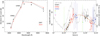 |
Fig. A.2. Left: Comparison of the time-averaged XMM-Newton OM spectrum from the current 2024 campaign with 2001 data. Right: Fluxes of different OM filters, scaled to the UVW1 filter, derived from the 2024 time-average spectrum. The best-fit phenomenological model is shown in red. The 0.3 − 0.6 keV X-ray light curve is overlaid for comparison. |
To construct a continuous light curve from the discontinuous photometric filter data, we calculated the average count rate ratios between UVW1 and the other filters, using the time-averaged data. This enabled us to scale the count rates from other filters to the UVW1 reference. In doing so, we assumed the optical/UV spectral shape remained constant during the observation, while the overall flux varied. As shown in Fig. A.2, the scaled data form a quasi-continuous light curve, capturing both the soft flare and a subsequent period. The scaled UVW1-equivalent count rate exhibits a smooth rise of approximately 6%, peaking at t ∼ 3 − 4 × 10⁵ s, followed by a gradual decline toward t ∼ 5 × 10⁵ s. To model this behavior, we fit the light curve with a smooth burst profile plus a constant component. The fit, shown in Fig. A.2, describes the light curve well, indicating a peak increase of 6.6 × 2.1% at 3.4 × 10⁵ s.
According to Mehdipour et al. (2017), the host galaxy contributes approximately 35% of the total UVW1 flux. Accounting for this, the observed increase in the OM flux corresponds to about 10% of the intrinsic UV disk flux. As shown in Fig. A.2, the OM light curve peaks with a delay of ∼1 × 10⁵ s relative to the peak of the flare in the 0.3 − 0.6 keV.
All Tables
All Figures
|
Fig. 1. XRISM Xtend light curves from the NGC 3783 campaign. Left: soft- and hard-band light curves, shown in black and red, respectively. The light curve has been binned to multiples of the XRISM orbit (5747 s), and in this paper we count time since the start of the XRISM observation. Right: X-ray variability surrounding the main soft flare at t ∼ 2.8 × 10⁵ s. |
| In the text | |
|
Fig. 2. Hardness ratio, defined by the count rates in the 3.0 − 6.0 keV and 0.3 − 0.6 keV bands, plotted against their combined count rate. Each data point represents a single XRISM orbit (5747 s). The data are color-coded by flare phase: pre-flare (black), rise (red), decay (blue), after-flare (magenta), and post-flare (orange). Gray points indicate observations outside the main soft flare. |
| In the text | |
|
Fig. 3. Time evolution of the NGC 3783 Resolve spectra. Top: average spectrum over all flare phases. Middle: spectrum during the decay phase only. Bottom: average spectrum combining all periods outside the soft flare, shown for comparison. The dip at ∼8.4 keV is unique to the decay phase. The light blue curve in the middle panel shows the best-fit model excluding both the UFO and the 3700 km s−1 components. |
| In the text | |
|
Fig. 4. Detailed look at the dip at 8.4 keV and the LEE. Left: Resolve, Xtend, NuSTAR, and XMM-Newton pn spectra from the decay phase. The red line shows the best-fit model to the Resolve data and including the UFO component, while the light blue line represents the model without it. Right: ΔC distribution from 1.3 × 10⁵ runs of the Monte Carlo simulation of the Resolve spectrum, and 1 × 10⁴ times for each of other three instruments (black histograms) and the observed ΔC distribution for the Resolve data (red histograms). Vertical lines mark the observed ΔC values for the other three instruments. |
| In the text | |
|
Fig. 5. Phase-resolved Resolve spectra during the soft flare. The best-fit models are shown in red. The light blue curves show the model that excludes both the UFO and the 3700 km s−1 component. |
| In the text | |
|
Fig. 6. Potential features identified with the pion scan on the Resolve data. The curves show the ΔC obtained in each step of the scan. The most prominent feature in each phase is highlighted with a thick line. In the bottom panel, all individual curves from the upper panels are combined and presented on a common ΔC scale for comparison. |
| In the text | |
|
Fig. 7. LEE in the pion scan. The black histogram shows the combined ΔC distribution from the rise, decay, after, and post-flare phases. The blue line represents an exponential fit to this histogram, following a form similar to that described in Sect. 2.3.2. The dashed red lines mark the ΔC values of the most prominent features identified in these phases. |
| In the text | |
|
Fig. 8. Evolution of outflow parameters during the flare. Left: outflow parameter. Middle: column density. These two panels are overlaid with the soft-band (black) and hard-band (red) X-ray light curves. A horizontal dashed line in the middle panel indicates the average column density excluding the decay phase. Right: column density as a function of the covering factor for the decay phase. |
| In the text | |
|
Fig. 9. Constraints on the density and distance of the outflow. Top: schematic illustrating a simple scenario: a clumpy outflow stream moving vertically from near the accretion disk, with the clump represented by the circle. Bottom: Density (left) and distance (right) constraints derived from the geometrical limits (nlow and Rupp) and escape velocity (nesc and Resc). Stars mark the density and distance values assuming that a clumpy component, observed during the decay phase, was launched at the pre-flare onset. The dashed line shows the density and distance limits estimated from the duration of the 8.4 keV dip during the decay phase. |
| In the text | |
|
Fig. 10. Comparison of UFO and CME dynamics. Left: evolution of the UFO velocity (in black). Middle: evolution of the UFO acceleration (in orange). Both panels are overlaid with the XMM-Newton OM (blue), soft-band (gray), and hard-band (red) X-ray light curves. Right: schematic view of the early dynamic evolution of a typical CME event close to the Sun, adapted from Temmer (2016). We see that the UFO and CME patterns are similar to each other, with the acceleration phase aligning with the hard-band flare and the velocity correlating with the soft-band flare. |
| In the text | |
|
Fig. A.1. Histogram of ΔC distributions for Resolve. The black histogram shows the results from 1.3 × 10⁵ Monte Carlo simulations per phase, and the observed distribution is shown in red. Vertical lines mark the positions of the best-fit features. |
| In the text | |
|
Fig. A.2. Left: Comparison of the time-averaged XMM-Newton OM spectrum from the current 2024 campaign with 2001 data. Right: Fluxes of different OM filters, scaled to the UVW1 filter, derived from the 2024 time-average spectrum. The best-fit phenomenological model is shown in red. The 0.3 − 0.6 keV X-ray light curve is overlaid for comparison. |
| In the text | |
Current usage metrics show cumulative count of Article Views (full-text article views including HTML views, PDF and ePub downloads, according to the available data) and Abstracts Views on Vision4Press platform.
Data correspond to usage on the plateform after 2015. The current usage metrics is available 48-96 hours after online publication and is updated daily on week days.
Initial download of the metrics may take a while.