| Issue |
A&A
Volume 705, January 2026
|
|
|---|---|---|
| Article Number | A100 | |
| Number of page(s) | 29 | |
| Section | Interstellar and circumstellar matter | |
| DOI | https://doi.org/10.1051/0004-6361/202554764 | |
| Published online | 13 January 2026 | |
ALMAGAL
V. Relations between the core populations and the parent clump physical properties
1
INAF – IAPS,
via Fosso del Cavaliere, 100,
00133
Roma, Italy; Istituto Nazionale di Astrofisica (INAF)-Istituto di Astrofisica e Planetologia Spaziali, Via Fosso del Cavaliere 100,
00133
Roma,
Italy
2
Dipartimento di Fisica, Sapienza Università di Roma,
Piazzale Aldo Moro 2,
00185
Roma,
Italy
3
Institut de Ciències de l’Espai (ICE, CSIC), Campus UAB, Carrer de Can Magrans s/n,
08193
Bellaterra (Barcelona),
Spain
4
Institut d’Estudis Espacials de Catalunya (IEEC),
08860
Castelldefels (Barcelona),
Spain
5
Dipartimento di Fisica, Università di Roma Tor Vergata,
Via della Ricerca Scientifica 1,
00133
Roma,
Italy
6
Physikalisches Institut der Universität zu Köln,
Zülpicher Str. 77,
50937
Köln,
Germany
7
SKA Observatory, Jodrell Bank, Lower Withington,
Macclesfield
SK11 9FT,
UK
8
Istituto Nazionale di Astrofisica (INAF), Osservatorio Astrofisico di Arcetri,
Largo E. Fermi 5,
Firenze,
Italy
9
Max Planck Institute for Astronomy,
Königstuhl 17,
69117
Heidelberg,
Germany
10
Institute of Astronomy and Astrophysics, Academia Sinica,
11F of ASMAB, AS/NTU No. 1, Sec. 4, Roosevelt Road,
Taipei
10617,
Taiwan
11
Jodrell Bank Centre for Astrophysics, Department of Physics and Astronomy, The University of Manchester,
Oxford Road,
Manchester
M13 9PL,
UK
12
Universität Heidelberg, Zentrum f|"ur Astronomie, Institut für Theoretische Astrophysik,
Albert-Ueberle-Str. 2,
69120
Heidelberg,
Germany
13
Universität Heidelberg, Interdisziplinäres Zentrum für Wissenschaftliches Rechnen,
Im Neuenheimer Feld 205,
69120
Heidelberg,
Germany
14
Harvard-Smithsonian Center for Astrophysics,
60 Garden Street,
Cambridge,
MA
02138,
USA
15
Elizabeth S. and Richard M. Cashin Fellow at Radcliffe Institute for Advanced Studies at Harvard University,
10 Garden Street,
Cambridge,
MA
02138,
USA
16
Faculty of Physics, University of Duisburg-Essen,
Lotharstraße 1,
47057
Duisburg,
Germany
17
Université Paris-Saclay, Université Paris-Cité, CEA, CNRS, AIM,
91191
Gif-sur-Yvette,
France
18
Jet Propulsion Laboratory, California Institute of Technology,
4800 Oak Grove Drive,
Pasadena,
CA
91109,
USA
19
School of Physics and Astronomy, University of Leeds,
Leeds
LS2 9JT,
UK
20
Department of Astronomy, School of Science, The University of Tokyo,
7-3-1 Hongo, Bunkyo,
Tokyo
113-0033,
Japan
21
SRON Netherlands Institute for Space Research,
Landleven 12,
9747,
AD
Groningen,
The Netherlands
22
Kapteyn Astronomical Institute, University of Groningen,
Landleven 12,
9747
AD
Groningen,
The Netherlands
23
INAF-Istituto di Radioastronomia & Italian ALMA Regional Centre,
Via P. Gobetti 101,
40129
Bologna,
Italy
24
Centro de Astro-Ingeniería UC, Instituto de Astrofísica, Pontificia Universidad Católica de Chile, Avda Vicuña Mackenna
4860,
Macul, Santiago,
Chile
25
Max-Planck-Institut für Radioastronomie,
Auf dem Hügel 69,
53121
Bonn,
Germany
26
University of Connecticut, Department of Physics,
196A Auditorium Road, Unit 3046,
Storrs,
CT
06269,
USA
27
East Asian Observatory,
660 N. A’ohoku, Hilo,
Hawaii,
HI
96720,
USA
28
UK Astronomy Technology Centre, Royal Observatory Edinburgh,
Blackford Hill,
Edinburgh
EH9 3HJ,
UK
29
Dipartimento di Fisica e Astronomia, Università degli Studi di Firenze,
Via G. Sansone 1,
50019
Sesto Fiorentino, Firenze,
Italy
30
Departamento de Astronomía, Universidad de Chile,
Casilla 36-D,
Santiago,
Chile
31
Max-Planck-Institute for Extraterrestrial Physics (MPE),
Garching bei München,
Germany
32
LUX, Observatoire de Paris, Université PSL, Sorbonne Université, CNRS,
75014
Paris,
France
33
Shanghai Astronomical Observatory, Chinese Academy of Sciences,
80 Nandan Road,
Shanghai
200030,
China
34
Leiden Observatory, Leiden University,
PO Box 9513,
2300
RA
Leiden,
The Netherlands
35
National Radio Astronomy Observatory,
520 Edgemont Road,
Charlottesville,
VA
22903,
USA
36
School of Engineering and Physical Sciences, The University of Lincoln, Brayford Way,
Lincoln
LN6 7TS,
UK
37
INAF – Astronomical Observatory of Capodimonte,
Via Moiariello 16,
80131
Napoli,
Italy
38
Dipartimento di Fisica e Astronomia, Alma Mater Studiorum – Università di Bologna Dipartimento di Fisica e Astronomia “Augusto Righi”,
Via Gobetti 93/2,
40129,
Bologna,
Italy
39
Center for Data and Simulation Science, University of Cologne,
Germany
40
Research Center for Astronomical computing, Zhejiang Laboratory,
Hangzhou,
China
41
Universidad Autonoma de Chile,
Av Pedro de Valdivia 425, Providencia,
Santiago de Chile,
Chile
★ Corresponding author: This email address is being protected from spambots. You need JavaScript enabled to view it.
Received:
26
March
2025
Accepted:
7
November
2025
Abstract
Context. The fragmentation of massive molecular clumps into smaller, potentially star-forming cores plays a key role in the processes of high-mass star formation. The ALMAGAL project, using the Atacama Large Millimeter/submillimeter Array (ALMA), offers highr-esolution data to investigate these processes across various evolutionary stages in the Galactic plane.
Aims. This study aims at correlating the fragmentation properties of massive clumps, obtained from ALMA observations, with their global physical parameters (e.g., mass, surface density, and temperature) and evolutionary indicators (e.g., luminosity-to-mass ratio and bolometric temperature) obtained from Herschel observations. It seeks to assess whether the cores evolve in number and mass in tandem with their host clumps and to determine the possible factors influencing the formation of massive cores (M > 24 M⊙).
Methods. We analyzed the masses of 6348 fragments, estimated from 1.4 mm continuum data for 1007 ALMAGAL clumps. Leveraging this unprecedentedly large dataset, we evaluated statistical relationships between clump parameters, estimated over ~0.1 pc scales, and fragment properties, corresponding to scales of a few thousand astronomical units, while accounting for potential biases related to distance and observational resolution. Our results were further compared with predictions from numerical simulations.
Results. The fragmentation level correlates preferentially with clump surface density, supporting a scenario of density-driven fragmentation; however, it does not show any clear dependence on total clump mass. Both the mass of the most massive core and the core formation efficiency exhibit a broad range and increase, on average, by an order of magnitude across intervals defined by evolutionary indicators such as clump-dust temperature and the luminosity-to-mass ratio. This suggests that core growth continues throughout clump evolution, favoring clump-fed over core-fed theoretical scenarios. However, significant scatter in these relationships indicates that multiple factors, including magnetic fields, turbulence, and stellar feedback, not quantifiable with continuum data, influence fragmentation, as also suggested by comparison with numerical simulations.
Key words: methods: observational / techniques: interferometric / stars: formation / ISM: clouds / ISM: structure / submillimeter: ISM
© The Authors 2026
 Open Access article, published by EDP Sciences, under the terms of the Creative Commons Attribution License (https://creativecommons.org/licenses/by/4.0), which permits unrestricted use, distribution, and reproduction in any medium, provided the original work is properly cited.
This article is published in open access under the Subscribe to Open model. This email address is being protected from spambots. You need JavaScript enabled to view it. to support open access publication.
1 Introduction
Understanding the processes that drive the formation of massive stars still represents a key challenge in astronomy, with several critical issues still under debate (Tan et al. 2014; Motte et al. 2018). For instance, it is still unclear how mass accumulates to form a high-mass star, whether specific physical conditions are required for this process, and whether high-mass stars form in conjunction with massive clusters–and, if so, how they influence the subsequent formation of surrounding stars.
The fragmentation of massive condensations (clumps, with diameters ranging from ~0.3 and 3 pc, e.g., Bergin & Tafalla 2007) within molecular clouds plays a pivotal role in the formation of stellar clusters and massive stars, shaping the morphology of their host clouds. This process is not regulated solely by gravity; turbulence (Klessen 2001; Elmegreen 2002; Nakamura & Li 2005; Zhang et al. 2009; Wang et al. 2014; Dunham et al. 2016), magnetic fields (Basu et al. 2009; Hennebelle et al. 2011; Fontani et al. 2016; Beltrán et al. 2019; Añez-López et al. 2020; Palau et al. 2021; Beuther et al. 2024), and protostellar feedback (Krumholz & McKee 2008; Krumholz et al. 2010; Guszejnov et al. 2017; Menon et al. 2024; Sanhueza et al. 2025) also play an important role in counteracting gravity and influencing fragmentation.
Recent advancements in millimeter interferometry have enabled high-resolution imaging capable of spatially resolving the internal structure of clumps that are candidates for massive star formation precursors or active sites of massive star formation. These observations allow direct comparisons with theoretical models. Specifically, dust continuum observations provide valuable insights into clump fragmentation and the masses of resulting fragments. The sizes of these smaller-scale condensations, as resolved by modern interferometers, generally correspond to those of the cores, typically ranging from 0.03 to 0.2 pc (see Bergin & Tafalla 2007).
Fragmentation is a dynamic, time-evolving process, so it is essential to characterize observed targets based on their evolutionary stage. Particular attention has been given to objects selected as representatives of the earliest phases of star formation or those still in a quiescent state. These have been observed using the Submillimeter Array (SMA, Zhang et al. 2009; Wang et al. 2014; Sanhueza et al. 2017), the Atacama Compact Array (ACA, Csengeri et al. 2017), the Atacama Large Millimeter Array (ALMA, Sanhueza et al. 2019; Svoboda et al. 2019; Anderson et al. 2021; Morii et al. 2023), and the Northern Extended Millimeter Array (Rigby et al. 2024).
Other studies have focused on star-forming clumps in more advanced stages. Using ALMA, Liu et al. (2020, 2024) and Xu et al. (2024b) surveyed more than a hundred candidate ultracompact (UC) HII regions, while Xu et al. (2024a) observed 11 massive protoclusters.
Several studies have aimed to cover a broad range of evolutionary stages. These include work by Palau et al. (2013) with the Plateau de Bure Interferometer (PdBI), Beuther et al. (2018a) with NOEMA, (Motte et al. 2022; Olmi et al. 2023; Traficante et al. 2023; Avison et al. 2023; Cheng et al. 2024; Ishihara et al. 2024) with ALMA, and Pandian et al. (2024) with SMA. These observing programs, based on target samples ranging from a few to 146 sources, are summarized in Table 1.
A major step toward a statistical approach to clump fragmentation, covering a wide range of physical conditions and Galactic locations, is represented by ALMAGAL (ALMA Cycle 7 large project; PI: S. Molinari, P. Schilke, C. Battersby, and P. Ho). This survey observed both continuum and line emission down to a scale of 1000 au, targeting a sample of 1017 clumps in the Galactic plane (Molinari et al. 2025; Sánchez-Monge et al. 2025), selected from the catalogs of two far-infrared continuum surveys: the Herschel1 Far-Infrared Galactic Plane Survey (Hi-GAL, Molinari et al. 2010; Elia et al. 2017, 2021), and the Red MSX Source (RMS, Lumsden et al. 2013). The catalog by Coletta et al. (2025), which reports the cores extracted from ALMAGAL continuum maps, represents an important dataset for studying the fragmentation in these clumps.
In this paper, we investigate correlations between key physical properties describing the core populations in ALMAGAL clumps – particularly those quantifying the fragmentation level and the potential for massive star formation – and the clump’s large-scale photometric and physical parameters. The analysis of the mass distribution of cores and their spatial arrangement lies beyond the scope of this study and is addressed in the works by Coletta et al. (2025) and Schisano et al. (2025), respectively.
To interpret our results, we compare our observations with leading high-mass star formation theories, broadly categorized into “core-fed” and “clump-fed” scenarios, based on the mechanisms responsible for mass accumulation. The core-fed model posits that massive stars originate from individual, preexisting gas cores with masses already established at the early fragmentation (e.g., McKee & Tan 2002, 2003). In this scenario, a massive core accumulates material in a quasi-static manner, gradually accreting onto a single protostar. In contrast, the clump-fed scenario envisions star formation in a dynamic, clustered environment where gas is accreted from a larger-scale clump. Models such as competitive accretion (Bonnell et al. 2001), global hierarchical collapse (GHC, Vázquez-Semadeni et al. 2019), and inertial flow (Padoan et al. 2020) fall under this category. In this scenario, gas flows into the protostellar vicinity through accretion streams rather than from a single core, enabling continuous mass accretion that supports growth beyond the initial core mass (e.g., Klessen 2001). In the current paper, we critically compare model predictions of the number and mass distribution of fragments as functions of environmental density and star formation age with our observational findings. As it is instructive to compare observations with numerical simulations of collapsing clumps (e.g., Fontani et al. 2018), we incorporate state-of-the-art simulations by Lebreuilly et al. (2025) into our analysis, focusing on the case of a 500 M⊙ magnetized clump, and comparing the number and total mass of the resulting sink particles during its evolution to the fragmentation level and formation efficiency observed in ALMAGAL clumps, respectively.
The structure of this paper is as follows: Sect. 2 outlines the set of parameters used in the analysis. In Sections 3, 4, and 5, we compare the degree of fragmentation in terms of the number of detected cores, the mass of the most massive core (MMC), and the core formation efficiency (CFE), respectively, against clump properties. In Sect. 6, we present additional combinations of parameters to discuss the possible interplay of physical conditions responsible for the observed fragmentation properties. Finally, in Sect. 7 we draw our conclusions.
Summary of recent studies on clump fragmentation carried out on interferometric data of continuum emission.
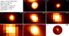 |
Fig. 1 Example of an ALMAGAL target observed from mid-infrared to millimeter. The ALMAGAL ID (AG323.7408-0.2633), its physical parameters (Molinari et al. 2025), and the number of cores detected in ALMAGAL continuum observations (Coletta et al. 2025) are reported in the top-left corner of the figure. Panels a–h: source images (~80″ × 45″) at wavelengths increasing from 24 μm to 1.38 mm. The wavelength in micrometers is reported in the top-right corner of each panel. Panel a: Spitzer-MIPS image of the source (saturated in the center). Panels b and c: Herschel-PACS images. Panels d–f: Herschel-SPIRE images. Panel g: the ATLASGAL image. Panel h: new ALMAGAL image. In this image, 15 fragments were detected by Coletta et al. (2025). Angular resolutions in the different panels are as follows: a: 6″; b: 10.2″ (for this panel and the following four, the resolution value is not the nominal one for Herschel, but rather the one directly measured by Traficante et al. 2011, on Hi-GAL maps, and circularized here); c: 13.5″; d: 23″; e: 30″; f: 42″; g: 19″; and h: 0.5″. Being detected at 70 μm (and also at 24 μm, in this case), this source is classified as star-forming in accordance with the Hi-GAL catalog criteria. |
2 A premise on clump and core properties
2.1 Clump physical parameters
Of the 1017 targets initially present in the ALMAGAL observing plan, 1007 are analyzed in this work. Indeed, Molinari et al. (2025) ruled out four fields due to incorrect target selection or duplication of observations. Additionally, they identified six clumps for which determining physical properties from Hi-GAL data (see below) is not feasible, so these targets are excluded from the present analysis.
For these 1007 objects, physical properties were calculated from Hi-GAL photometry (an example is shown in Figure 1). For the subsample of sources selected directly from the Hi-GAL catalog, we used data from Elia et al. (2021). Based on the physical sizes obtained using the distances estimated by Mège et al. (2021) for ~80% of the entries in the catalog of Elia et al. (2021), it can be affirmed that most of these sources can be classified as clumps.
In Elia et al. (2017, 2021), Hi-GAL clump photometry at 70, 160, 250, 350, and 500 μm was supplemented, where possible, with flux densities at 21, 22, 24, 870, and 1100 μm from MSX (Egan et al. 2003), WISE (Wright et al. 2010), MIPSGAL (Gutermuth & Heyer 2015), ATLASGAL (Schuller et al. 2009), and BGPS (Rosolowsky et al. 2010; Aguirre et al. 2011) surveys, respectively. Sources detected at 70 μm were classified as “star-forming” (as the example shown in Figure 1). In contrast, those undetected at 70 μm-dark were classified as quiescent. The ALMAGAL sample is divided into 891 star-forming and 116 quiescent sources, respectively.
A modified blackbody (e.g., Elia & Pezzuto 2016) with a mass opacity coefficient (hereafter opacity) of κ300 = 10 cm2 g−1 at 300 μm equivalent to 0.1 cm2 g−1 after including a gas-to-dust ratio of 100 Hildebrand (1983), and a spectral index β = 2 was fit to the portion of the spectral energy distribution (SED) at wavelengths λ ≥ 160 μm, to derive temperatures and, where heliocentric distances were available, to estimate masses as well. In this respect, the cataloged temperature represents an average value, dominated by the colder dust present in the outer regions of the clump, and only partially reflecting any potential star formation activity in its inner regions. Correspondingly, the derived mass represents the total mass of the clump, predominantly contained within its large-scale envelope. As a result, the surface density, estimated as the ratio of clump mass to area, provides an average value that does not account for the highly inhomogeneous internal structure expected within a clump. It is noteworthy that in Elia et al. (2017, 2021), the surface density was calculated using the beam-deconvolved, circularized size of the source at 250 μm. In some cases, this method results in extremely high surface densities (Σ ≫ 10 g cm−2), which are not comparable with similar ALMA studies using non-deconvolved sizes (e.g., Morii et al. 2023). For this reason, in this work, we chose to base our discussion of clump surface densities on non-deconvolved sizes. These densities are, by definition, higher than those derived using deconvolved sizes, with the average ratio of the two being 0.56, and a standard deviation 0.18.
The clump bolometric luminosity was obtained as the sum of the integral under the observed SED at λ ≤ 160 μm (if available) and the integral under the best-fitting modified blackbody at λ > 160 μm. The ratio of bolometric luminosity and mass, which is distance-independent, is generally considered a suitable descriptor of the clump evolution (e.g., Molinari et al. 2008, 2016; Smith 2014; Elia et al. 2017) and is used in the current paper as such. At first glance, including both the dust temperature T and the L/M parameter in our analysis may seem redundant, as the two show a good degree of correlation (Elia et al. 2017; Urquhart et al. 2018). However, they are estimated from different datasets, as T is derived from fluxes at λ ≥ 160 μm, while L derives from the integral of the SED extended to shorter wavelengths. This accounts for the spread observed in the aforementioned relation between these two quantities. For this reason, and to facilitate future comparisons with the outputs of possible numerical simulations, we prefer to retain both quantities in our analysis. We also make use of the bolometric temperature, defined by Myers & Ladd (1993) as a weighted average frequency (converted into a temperature) of the observed SED and estimated as described in Elia et al. (2017), as a powerful evolutionary tool.
Once ALMAGAL spectroscopic data became available, it was possible to reconsider the radial velocities quoted by Mège et al. (2021) to ALMAGAL targets. Consequently, heliocentric distances were updated by Benedettini et al. (in prep.) using radial velocities directly extracted from ALMAGAL line observations to obtain an updated and self-consistent set of parameters. Hence, rescaled distance-dependent quantities were listed by Molinari et al. (2025).
Furthermore, for the portion of the ALMAGAL target list directly selected from the RMS survey (Lumsden et al. 2013), rather than from Hi-GAL, Molinari et al. (2025) made an effort to identify possible Hi-GAL counterparts and to derive their physical parameters. We refer to Molinari et al. (2025) for further details on this recovery procedure. As mentioned above, this procedure was not applicable to the six targets, which were therefore excluded from the present analysis.
To enrich the evolutionary characterization of ALMAGAL targets, we searched for possible compact or UC HII (UCHII) region counterparts in the source catalogs of the radio surveys CORNISH (Purcell et al. 2013, obtained for the coordinate range 10° < ℓ < 65°, |b| < 1°) and CORNISH South (Irabor et al. 2023, 295° < ℓ < 350°, |b| < 1°). A total of 340 and 526 ALMAGAL targets fall within the coverage of the former and latter surveys, respectively. Adopting a searching radius of 10″, 24 and 50 matches with ALMAGAL were found in the former and the latter, respectively. As expected, all matched sources are detected at 70 μm, confirming that they constitute a subsample of the star-forming clump class. In the following, UCHII region counterparts are treated as a separate class with respect to that of the generic star-forming clumps.
Figure 2 shows the statistics of clump physical properties, separately for different evolutionary classes (quiescent, star-forming, UCHII region candidates). The initial requirements for selecting the Hi-GAL-selected subsample included a M > 500 M⊙ constraint, so that the presence of smaller masses in the current list of ALMAGAL target properties is due to part of the RMS-selected targets, as well as to Hi-GAL-selected targets for which an update of distance produced a substantial change in mass. As highlighted by Elia et al. (2017, 2021), the evolutionary indicators (dust temperature, L/M, and bolometric temperature) are generally found to be enhanced in star-forming clumps, especially in those associated with compact radio emission.
Remarkably, also after the inclusion of the cross-match with the CORNISH South catalog, a large fraction (83%) of the targets recognized as UCHII region candidates have L/M above 10 L⊙/M⊙, confirming the trend highlighted by Urquhart et al. (2013) and Cesaroni et al. (2015). In particular, 68% of them fulfill the threshold of 22.4 L⊙/M⊙ suggested by Elia et al. (2017) as a conservative requirement for compatibility with the presence of a HII region.
Finally, a further examination of the classification between quiescent and star-forming clumps, considering the specific positions observed in ALMAGAL, is essential. In many star-forming Hi-GAL clumps, a systematic shift in the position of the emission peak across Herschel bands, from 70 to 500 μm, is observed. It can be shown that this migration is intrinsic rather than a result of resolution effects or incorrect astrometric alignment (Elia et al., in prep.). Near-infrared images of these objects often reveal clusters of young stellar objects (YSOs) coinciding with the 70 μm peak. In contrast, emission at SPIRE wavelengths (250–500 μm) generally originates from a near infrared (NIR)-dark region alongside. Consequently, for these sources, the SED collected from the five Hi-GAL bands reflects contributions from spatially connected but physically distinct components. For the Hi-GAL-selected ALMAGAL targets, the ALMA observations were centered on the 250-μm peak position. Therefore, in cases where the angular separation between the 70 μm and 250 μm peaks approaches or exceeds the ALMAGAL field of view (FOV) radius (~17.5″), the ALMAGAL images may capture the quiescent portion of a clump rather than the star-forming region itself. In the ALMAGAL sample, this separation exceeds 15″ for 11 sources, and 18″ for three of these. While these numbers reflect a bias that must be carefully taken into account when analyzing individual sources, their possible influence on overall trends for object classes can be considered statistically negligible.
2.2 Core physical parameters
The morphologic, photometric, and physical properties of fragments detected in ALMAGAL continuum observations were determined by Coletta et al. (2025). The images were produced by combining data from various ALMA configurations (see Sánchez-Monge et al. 2025). Specifically, the compact configurations C-2 and C-3 (collectively referred to as TM2), and the extended configurations C-5 and C-6 (summarized as TM1) were combined with data from the 7 m array of the Atacama Compact Array (ACA, referred to as 7 M). For this reason, the final products considered by Coletta et al. (2025) are called 7M+TM2+TM1 maps.
Heliocentric distances of all cores in a given target are assumed to be the same as the global target distance, assigned as mentioned in Sect. 2.1. Based on the distances available at the time of the ALMA proposal, targets were divided into two samples, to be observed with different configurations of the interferometer to preserve some uniformity in spatial resolution: the “near” distance for d ≤ 4.66 kpc (C2+C5 configurations, 476 targets observed), and the “far” distance for d > 4.66 kpc (C3+C6 configurations, 531 targets observed). The reassessment of distances by Benedettini et al. (in prep.) implied, in a minority of cases, that sources initially observed in the “far” configuration were reassigned a “near” distance, and vice versa. Details are provided by Molinari et al. (2025), Benedettini et al. (in prep.), and Coletta et al. (2025).
The fragment2 detection and photometry in the ALMAGAL fields were carried out with the CuTEx algorithm (Molinari et al. 2011), specifically adapted to the ALMAGAL maps, as detailed in Coletta et al. (2025). CuTEx performs background estimation and subtraction to derive final flux density measurements. Consequently, direct comparisons with core flux densities extracted in other similar ALMA surveys (e.g., Sanhueza et al. 2019; Svoboda et al. 2019; Anderson et al. 2021; Morii et al. 2023) are not straightforward, as those studies include background emission, leading to systematically higher flux density estimates compared to ALMAGAL.
Here, we briefly summarize the overall morphologic features of the cataloged cores, as presented by Coletta et al. (2025). The angular sizes range from 0.15″to 1.4″, with some distinction between the targets observed with the “near” configuration (for which the median angular size is ~0.4″) and the “far” one (median: ~0.2″; best: ~0.15″), respectively. Coupled with distances, this results in a physical size distribution whose 90% is contained in the range 800–3000 au, with a median of 1700 au.
The extracted ALMAGAL flux densities were converted into masses through the modified blackbody formula, assuming an opacity of 0.9 cm2 g−1 at 1.3 mm, suitable for dense environments (Ossenkopf & Henning 1994; Sanhueza et al. 2019), a gas-to-dust ratio of 100 (not included in the aforementioned opacity), and a temperature Tcore established according to the following scheme based on the L/M ratio of the parent clump: Tcore = 20 K for L/M ≤ 1 L⊙/M⊙; Tcore = 35 K for 1 L⊙/M⊙ < L/M ≤ 10 L⊙/M⊙; Tcore ∝ (L/M)0.22 for L/M > 10 L⊙/M⊙, respectively (see Coletta et al. 2025, for details). Core masses are found in the range 0.002–345 M⊙, with a mean value of 1.5 M⊙ and a median of 0.4 M⊙. The 90% flux completeness in the catalog is 0.95 mJy, which translates into 0.13 and 0.37 M⊙ at d = 3.5 and 6 kpc, respectively.
Coletta et al. (2025) investigated whether core flux densities, and consequently core masses, can be overestimated due to contamination by free-free emission. They considered the possible presence of CORNISH and CORNISH South emission (including diffuse emission, not just the compact emission mentioned in Sect. 2.1) within the ALMAGAL fields. Through this approach, they identified 110 targets where at least one core photometry might be affected by such contamination. In Appendix D, we focus on the subsample of ALMAGAL targets confirmed to be free from this contamination. Moreover, we demonstrate that trends observed in the relationships between target properties generally remain unchanged, whether the analysis is performed on this subset or the entire sample.
Finally, we summarize here the approach of Baldeschi et al. (2017) in linking Herschel clump properties to those of the cores they contain, whose results are frequently referenced throughout this paper. To study distance bias in Hi-GAL clump measurements and clump-core connections, they simulated observing nearby (150–500 pc) star-forming regions mapped in the Herschel Gould Belt survey (André et al. 2010) at distances up to 7 kpc by progressively degrading their resolution. At each simulated distance, they re-extracted sources and recalculated physical parameters, comparing them to the original data. This approach revealed how distance affects Herschel-based observables. Similarly, the resolution improvement from Herschel clumps to ALMAGAL fragments discussed in the current paper mirrors the relationship between a clump observed in a map artificially degraded by Baldeschi et al. (2017) to kiloparsec distances and the cores detected in the original Gould Belt map (see also Appendix B).
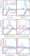 |
Fig. 2 Distributions of ALMAGAL target physical properties: (a) heliocentric distance; (c) mass (common logarithm); (e) surface density (common logarithm); (g) bolometric luminosity over mass ratio (common logarithm); (i) modified blackbody temperature; and (k) bolometric temperature. Panels b, d, f, h, j, and l: corresponding cumulative distributions. Three different populations are shown separately: in red, quiescent (70-μm dark) clumps; in blue, star-forming (70-μm bright) clumps; and in cyan, star-forming clumps associated with an UC HII region (notice that, differently from Elia et al. 2017, 2021, the counts of the third class of objects are not also included in those of the second class). All histograms are normalized by their total (116, 817, and 74 sources, respectively); therefore, they do not mirror the actual number ratios between clump classes. Units on the y-axis are arbitrary. Additionally, in the panels containing the cumulative distributions, the red and dotted curves correspond to the subsamples of quiescent and star-forming clumps with no detection of millimeter cores in ALMAGAL observations (discussed in Sect. 3.5). UCHII regions are not shown, as only one appears devoid of cores inside. |
3 Clump fragmentation level
In this section, we adopt a statistical approach to investigate the level of fragmentation in the ALMAGAL targets and explore its relationship with their photometric, physical, and evolutionary properties. The data are expected to reveal scattered distributions rather than clear-cut trends, indicating that multiple interacting factors contribute to determining the number of substructures within a fragmented clump. However, thanks to the statistical robustness offered by ALMAGAL, it is possible to identify average trends and to evaluate the potential impact of individual clump parameters.
3.1 Clump fragmentation versus photometry
The first question to address is whether it is possible to predict the internal fragmentation level of clumps from a macroscopic property, such as their brightness in the far-infrared. In the top of Figure 3, we investigate the relation between the number of fragments detected within the clumps, Ncore, and the clump Herschel flux densities in the five Hi-GAL bands, averaged in bins of Ncore. An overall increasing trend appears up to Ncore ~ 25, becoming more pronounced as the wavelength decreases from 500 to 160 μm. This is the range in which clump temperatures are estimated, and this imbalance among wavelengths is expected to be mirrored in the temperature distribution. In fact, in the middle of Figure 3, an increase in the average clump temperature derived from the SED-modified blackbody fit, estimated in bins of Ncore, is also seen up to Ncore ~ 25. In contrast, the region for Ncore ≳ 25 is statistically irrelevant, as Coletta et al. (2025) showed that, in this range, bins of ΔNcore = 1 get populated by fewer than ten clumps.
To investigate a possible bias with the distance d on the trends observed in the top panel of Figure 3, the mean flux densities multiplied by d2 (i.e., a quantity proportional to the monochromatic luminosity) are plotted versus the Ncore parameter in the bottom panel of the same figure. An increasing trend similar to that seen in the top panel (although more scattered and shallower) confirms a general correlation between the number of fragments in the clump and the clump brightness at all wavelengths. A higher number of cores appears to be genuinely correlated with increased fluxes. This correlation cannot be trivially attributed solely to the presence of more emitting objects but rather carries evolutionary implications (i.e., more evolved clumps tend, on average, to host a larger number of cores), as suggested by the middle panel of Figure 3 and further explored in Sections 3.4 and 6.2.
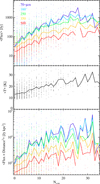 |
Fig. 3 Properties of ALMAGAL targets as a function of the number of cores (Ncore) revealed in their interior. Top: fluxes in the five Hi-GAL bands and their averages in bins of ΔNcore = 1. The core-band correspondence is reported in the legend. Middle: temperature determined using a modified-blackbody fit to the Hi-GAL SEDs and its average. Bottom: as in the top panel, but for the product of flux densities and the squared distance. In both the top and bottom panels, a break in the red curve corresponds to a bin populated by sources without a 500 μm detection. |
3.2 Clump fragmentation versus distance
In principle, the number of detected cores in ALMAGAL targets might be underestimated due to both sensitivity limitations and resolution loss at increasing target distances, leading to confusion and loss of lower-mass fragments. Therefore, the pure count of cores detected in a given field turns out to be a quantity more affected by the distance bias than, for instance, the total mass in cores.
In panel a of Figure 4, Ncore is plotted against distance. Despite a large scatter due to the intrinsic level of fragmentation in various clumps, a slightly decreasing trend is observed in the median of Ncore computed in 1 kpc bins of distance, at least within the interval 2 < d < 8 kpc, in which the statistical basis is rich enough (i.e., at least ten objects per bin), confirming a mild influence of the expected distance bias. However, within this range, no discontinuity is observed, in both the overall scatter plot and the median trend3, in correspondence of d = 4.66 kpc, namely the distance used to separate the two subsamples of ALMAGAL targets to be observed with different ALMA baseline configurations. Therefore, the decreasing trend of Ncore with distance appears a more direct consequence of the decrease in mass sensitivity, related to d−2, rather than in resolution (cf. Coletta et al. 2025). Finally, it is worth noting that analyzing Ncore as a function of distance-independent clump parameters, as in Sects. 3.3 and 3.4, mixes up the ordering of the clumps by distance, thereby mitigating the impact of the bias seen in this context.
3.3 Clump fragmentation versus mass and density
A search for a possible link between the fragmentation level of clumps and their total mass estimated with Herschel, namely the mass available for fragmentation, is illustrated in panel b of Figure 4. Confirming the results of Fontani et al. (2018), Olmi et al. (2023), and Traficante et al. (2023), no clear correlation is observed between these quantities, except for a mildly increasing median trend in the range of masses with higher statistics (500 ≲ M ≲ 2000 M⊙).
A more pronounced correlation is observed, instead, between median Ncore and clump surface density Σ (Figure 4, panel c). Unlike previous scatter plots, there is a noticeable increase in both the maximum and median Ncore values with rising surface density4. Additionally, for Σ > 2 g cm−2 instances of low fragmentation level (say Ncore ≤ 3) are almost absent. These aspects were glimpsed in more limited statistics (11 objects) by Svoboda et al. (2019). More recently, Morii et al. (2024) highlighted a similar correlation between Ncore and Σ in a sample of 39 targets. The ALMAGAL data further reinforce this trend, providing strong statistical significance.
On the one hand, the expression of classical Jeans’ mass has an inverse square-root dependence on volume density, suggesting that fragmentation into further supercritical substructures is favored in conditions of high density (for an assessment of the equivalence of a clump description based on volume or surface density see Appendix A). On the other hand, the theoretical prediction by Krumholz & McKee (2008) indicates that a surface density equal to or greater than 1 g cm−2 is a necessary, though not sufficient, threshold to inhibit further fragmentation, thus promoting high-mass star formation, when a cloud undergoes heating. However, there is no noticeable flattening of the median Ncore versus Σ trend around this value. Instead, such flattening might be glimpsed near 2 g cm−2, but in a less statistically significant region of the diagram.
We note that the behavior of Ncore versus surface density should not be overinterpreted in an evolutionary sense. On the one hand, Elia et al. (2017) showed that, on average, the surface density is larger in star-forming clumps than in quiescent ones; furthermore, among the star-forming population, the densest sources are, on average, those appearing dark at ~20 μm. However, since a high surface density was imposed as a constraint to select ALMAGAL targets, this is not necessarily true in the objects studied here (see Figure 2c). On the other hand, for sources with high L/M (≫ 10 L⊙/M⊙), expected to be the most evolved in the Hi-GAL catalog, a wide range of surface density values is observed, from high values typical of very concentrated envelopes to low ones that may correspond to clumps being cleaned up by internal protostellar activity. This aspect is further discussed in Appendix A. In this context, exploring the Ncore parameter as a function of the parent clump surface density cannot yield clear evolutionary indications, unlike other distance-independent parameters, such as T or L/M. This is confirmed in panel c of Figure 2 and in panel c of Figure 4 by the high degree of scattering shown by the HII regions along the x-direction. The differentiation in fragmentation trends as a function of clump surface density and evolutionary stage is discussed in further detail in Sect. 6.2.
3.4 Clump fragmentation versus evolutionary status
The development of fragmentation with time depends on local conditions, and consequently, the final distribution of masses can strongly vary from case to case. The statistics provided by ALMAGAL offer an interestingly varied picture of fragmentation as a function of clump evolutionary indicators.
The top of Figure 5 shows the distribution of Ncore in the ALMAGAL sample, divided into quiescent clumps, star-forming clumps, and UCHII regions. The UCHII regions exhibit a flatter distribution, with no strong preference for low Ncore values and a median5 of 14. In contrast, the distributions for the other two classes are qualitatively similar, with the histogram of star-forming clumps showing a stronger right skew than that of quiescent ones. The respective medians are 4 and 2, but a two-sample Kolmogorov–Smirnov (K–S) test was required to determine whether the differences between the datasets are statistically significant. In this case, the K–S statistic is D = 0.31, which must be compared with the critical value for rejecting, at a 99% confidence level, the null hypothesis that the two distributions are random samples from the same population. The critical value is given by
![Mathematical equation: $\[D_{m, n, 0.01}=1.63 \times \sqrt{\frac{m+n}{m n}},\]$](/articles/aa/full_html/2026/01/aa54764-25/aa54764-25-eq1.png) (1)
(1)
where m and n are the sizes of the two samples (e.g., Rohatgi & Saleh 2015). For this analysis, the sizes of the quiescent and star-forming clump subsamples are m = 83, n = 684, respectively, yielding D83,684,0.01 = 0.19. The fact that D is larger than this value indicates a statistically significant difference between the Ncore distributions for quiescent and star-forming clumps. Repeating the same exercise for a 99.87% confidence level, i.e., 3 sigma, increases the factor in Equation (1) to 1.92, and consequently increases D to 0.22, which remains below the K–S statistics obtained in this case.
The differences among these distributions become more evident if seen in terms of cumulative functions (Figure 5, bottom). The distribution for quiescent clumps appears more distinctly right-skewed compared to that of star-forming clumps. In contrast, UCHII regions show an almost linear trend over a wide range of Ncore, consistent with the nearly flat histogram.
Furthermore, we investigate whether the fact that several ALMAGAL star-forming targets lie outside the areas covered by the CORNISH and CORNISH South surveys can lead to significant contamination by UCHII regions. The bottom of Figure 5 shows the cumulative curve for star-forming targets within the coverage of these two surveys: this curve differs only negligibly from the overall cumulative distribution, indicating that any potential bias can be considered negligible both here and throughout the rest of the paper.
To obtain a further differentiation of clumps across different evolutionary stages, we discuss below the distribution of Ncore as a function of a few descriptors. Already in the middle panel of Figure 3, an average increase in temperature with Ncore suggests that a larger number of fragments is found in warmer objects.
In panel d of Figure 4, first we analyze the distribution of the number of detected fragments, Ncore, in each clump as a function of the clump L/M ratio. We observe that cases with few or no fragments appear across the entire range of L/M. However, the highest values of Ncore at different regimes of L/M tend to increase with this ratio. Specifically, clumps with low L/M (<1 L⊙/M⊙) reveal a relatively low number (less than ten) of detected cores, whereas higher numbers are increasingly found, in many cases, at larger L/M, thus suggesting a possible evolutionary implication.
This can be summarized in the overall increasing behavior of the median of Ncore in bins of log(L/M), at least for L/M < 100 L⊙/M⊙, in which the statistics are meaningful (more than ten sources per bin). Noticeably, such a trend was not found by Traficante et al. (2023), most likely due to a narrower range of L/M investigated, the much smaller statistics, and the coarser angular resolution (>1″). A further discussion of the relationship between Ncore and L/M in light of numerical simulations is provided in Sect. 6.2.
In panels e and f of Figure 4, Ncore is plotted against the clump dust temperature T and bolometric temperature Tbol, respectively. An increasing level of fragmentation corresponds, on average, to the increase in these two evolutionary indicators, confirming that which emerged from panel d. In the case of T, this may initially seem counterintuitive when considering, for example, the analytical form of the thermal Jeans mass. However, since clump temperature is strongly correlated with other evolutionary parameters (Elia et al. 2017), the observed increase in Ncore as a function of temperature should be regarded as an evolutionary effect rather than a “static” one. Specifically, while the clump’s average density and temperature reflect global conditions, local fluctuations within the clump can lead to lower Jeans masses, facilitating fragmentation. Over time, as a consequence of the global collapse of the clump, these conditions can be achieved in different regions of the clump, resulting in the formation of new fragments. In practice, barring significant episodes of core coalescence, Ncore is expected to increase monotonically with time, or at least to remain constant if strong feedback from newly formed YSOs effectively suppresses further fragmentation throughout the clump. Additionally, we cannot rule out the possibility of a selection effect, where warmer cores naturally exhibit higher continuum flux densities.
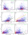 |
Fig. 4 Number of fragments Ncore detected in each ALMAGAL target as a function of the target’s physical parameters: (a) heliocentric distance, with the vertical dotted line separating the distances originally assigned to the “near” and the “far” sample (see text); (b) mass; (c) surface density (logarithm); (d) luminosity over mass ratio, with the orange line representing the model prediction from Lebreuilly et al. (2025) with initial conditions set to M = 500 M⊙, ℳ = 7, and μ = 10 (presented and discussed in Sect. 6.2.2); (e) modified blackbody temperature; and (f) bolometric temperature, respectively. The open red triangles represent quiescent clumps; open dark blue diamonds represent star-forming clumps; and light blue-filled circles represent counterparts of a UCHII region. The symbol under each panel represents the typical error bar associated with the data. In this case, the vertical error bar is replaced by an arrow to indicate the number of detected cores likely representing an underestimate of the “actual” Ncore. The green line connects the medians of Ncore in bins (whose width is specified in green as well); its dotted parts correspond to bins containing low statistics (less than ten values). In panel c, medians calculated in bins of surface densities but based on deconvolved clump sizes are also represented as a dark solid or dotted green line. The mean values are also shown, connected by a magenta line. |
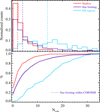 |
Fig. 5 Top: statistical distribution of the fragment number Ncore for the ALMAGAL targets, categorized into quiescent (red histogram), star-forming (blue), and CORNISH-based UCHII regions (light blue). The sum of each histogram is normalized to 1; therefore, all histograms subtend the same area and do not reflect the actual numerical proportions among the classes. The three vertical dashed lines indicate the medians of these distributions, calculated excluding cases where Ncore=0. Bottom: cumulative distributions corresponding to the histograms shown in the top panel. The cumulative distribution of Ncore for star-forming targets located within the regions covered by the CORNISH and CORNISH South surveys is also shown (dotted blue) to highlight the potential impact of contamination from UCHII regions (see text). |
3.5 Properties of clumps without core detections
Complementary to discussing the relations of the number of detected cores in ALMAGAL targets is the investigation of the statistics of parameters, both photometric and physical, for those targets in which Coletta et al. (2025) find no compact emission above 5 σ in the 7M+TM2+TM1 images. The distributions of Herschel flux densities for these sources are shown in the top and middle panel of Figure 6. In all bands, they are clearly centered on significantly lower values compared to the distributions of targets with detected cores. This trend is further highlighted in the bottom of Figure 6 by showing the cumulative distributions of the histograms displayed in the panels above, and quantified in Table 3, which reports lower median flux densities for these sources.
Note that the target heliocentric distance can influence the comparison of fluxes between clumps with and without cores. A lower Herschel flux in the absence of detected cores may reflect either the intrinsically faint nature of the clump or its large distance, as the sensitivity limit, which constrains the observed Ncore, follows the same d−2 dependence on distance. Rather than distinguishing between these scenarios, here we simply test for a possible link between the non-detection of cores and the relatively low flux in one or more Herschel bands.
In this respect, however, among the targets without cores, some cases with high flux densities (>100 Jy in one or more bands) remain. These cases, of course, cannot be explained as unfavorable occurrences of lower sensitivity. Indeed, we checked this by comparing the medians for the rms noise for fields without detected cores and for the subsample of those with F250 > 100 Jy, and for F350 > 100 Jy. In both cases, we find no difference in the distribution of rms values. These considerations prevent us from extracting a stringent recipe for possible lower limits on the Hi-GAL flux densities, ensuring the presence of bright cores inside the clump.
The ALMAGAL clumps without core detections show, in general, lower values of distance-independent parameters such as T, Σ, L/M, and Tbol, as illustrated in Table 3. Although distributions remain wide, clumps without core detection tend to be preferentially found among the less evolved or less dense subsets in the ALMAGAL sample.
For a deeper insight into this aspect, Figure 2 presents the cumulative distributions of the properties of clumps without core detections, shown separately for quiescent and star-forming ones. First, it should be noted that this statistics is based on 33 out of 116 quiescent clumps (28%), and 133 out of 817 star-forming clumps (16%), cf. Table 26. This provides a first indication of an evolutionary trend, non-detections occur more frequently in quiescent than in star-forming targets. In panels h, j, and l of Figure 2, the cumulative distributions of T, L/M, and Tbol, respectively, rise more steeply for clumps without cores than for the entire population, both for quiescent and star-forming clumps. This trend is even more evident for Σ (panel f), confirming what was suggested by the values in Table 3 for the whole ALMAGAL sample. In turn, this is consistent with the general picture that emerged for Ncore as a function of density and evolutionary state in Sects. 3.3 and 3.4, respectively.
Finally, panel b shows that, at least for star-forming clumps, distance can be responsible for a loss of sensitivity, as already discussed above, leading to an apparent increase in the number of cases with low Ncore, while mass does not appear to be systematically affected by this bias (panel d). In summary, the absence of detected cores in an ALMAGAL target may result from a joint effect of sensitivity and distance effects, or may be related to the clump density or evolutionary stage, or to a combination of these factors.
It is also necessary, at this stage, to consider two additional potential causes for the lack of core detections. The first is that the ALMAGAL target may in fact correspond to an evolved star or an external galaxy. A search in SIMBAD revealed only two cases without cores consistent with the former scenario, and none with the latter. The second possibility is that the ALMAGAL pointing, centered on the 250 μm emission peak, is significantly far from the 70 μm peak, causing the most densely core-populated region within the clump to be missed, as discussed in Section 2.1. However, as demonstrated in that section, the number of such cases is not statistically significant enough to produce general trends as those discussed in this section.
Younger, potentially pre-stellar cores, which often exhibit shallower and generally fainter intensity profiles (e.g., Beuther et al. 2002; Giannetti et al. 2013; Gómez et al. 2021), may be more likely to go undetected in the 7M+TM2+TM1 images, whose higher angular resolution results in worse brightness sensitivity (as highlighted by Sánchez-Monge et al. 2025). A scenario in which only such cores are present, ultimately resulting in observing Ncore = 0, is expected to occur in ALMAGAL clumps classified as quiescent. A detailed analysis of the ALMAGAL maps for fields without detected cores is beyond the scope of this paper and will be addressed in a forthcoming study by Coletta et al. (in prep.), through a dedicated analysis using only 7M+TM2 images to identify potential fragments not identified in 7M+TM2+TM1 observations. This approach aligns with the scenario presented here, as clumps with lower densities and/or early evolutionary indicators are likely candidates to host such early-stage cores.
Statistics of core population parameters (namely fragmentation level, mass of the MMC, and CFE).
Median photometric and physical parameters of the entire ALMAGAL sample and subsamples with and without cores.
4 Mass of the most massive core
The mass MMMC of the MMC in a clump is of great interest because it reflects a clump’s ability to concentrate matter and form a massive substructure. As a result of fragmentation, MMMC is inherently correlated with it and serves as a quantitative descriptor (e.g., Kirk et al. 2016; Lin et al. 2019; Sanhueza et al. 2019; Anderson et al. 2021; Morii et al. 2023). Another specific quantity that also accounts for the mass of the parental clump is the fraction fMMC of the clump mass contained within its MMC.
These quantities are analyzed below in relation to various clump properties. Despite significant scatter, some average trends emerge. On the one hand, this suggests that certain parameters may indeed influence the observed MMMC. On the other hand, it is evident that the observed values result from the complex interplay of multiple concomitant factors, making it challenging to disentangle their individual contributions.
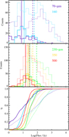 |
Fig. 6 Top: histograms of Hi-GAL PACS flux densities (dark blue: 70 μm; light blue: 160 μm) for ALMAGAL targets with and without the detection of cores (dotted and solid line, respectively). The median values for the two subsamples are shown as vertical dashed and solid lines of the same color, respectively. Middle: same as in the top panel, but for SPIRE flux density distributions (green: 250 μm; yellow: 350 μm; and red: 500 μm). Bottom: cumulative distributions of histograms shown in the top and middle panels, using the same color and line style convention. |
4.1 Mass of the most massive core versus distance
To investigate a possible distance bias in the estimation of the MMC mass, these two quantities are plotted in panel a of Figure 77. The points in the diagram exhibit significant scatter, and no overall increase in the median MMC mass can be observed across the 2 < d < 7 kpc range, where robust statistics are available, nor a break in slope at the separation between the “near” and the “far” subsamples.
Notably, for d > 10 kpc, we find MMMC > 5 M⊙. Further fragmentation of the MMC cannot be excluded in these cases if observed with better spatial resolution.
Despite these minor biases, the subsequent discussion of the MMC mass is not significantly affected. Specifically, the trends observed in the relationships between MMC mass and distance-independent clump parameters (Sects. 4.2, 4.3) appear uncorrelated with distance. For example, as a test, we recalculated all median trends of the other clump parameters shown in panels b to f of Figure 7 by considering only targets located at 2 kpc < d < 6 kpc. The medians based on this subsample exhibit trends identical to those obtained for the full sample and are, over extended ranges, even indistinguishable from them. Thus, while distance bias may introduce some scatter into these plots, it does not impose a systematic effect.
4.2 Mass of the most massive core versus clump mass and density
In panel b of Figure 7, the MMMC detected in each clump is plotted against the total clump mass. A large scatter is found, with a Spearman’s rank correlation coefficient ρS = 0.34. The significance levels of 5% and 0.03% (i.e., 3σ) correspond to critical values ρcrit =0.07 and 0.13, respectively, while 0.34 would correspond to a p-value of ~10−24, so that one might conclude a direct correlation between the two quantities. However, given the discussion in Section 6.1 about the significance of Spearman’s critical values in the presence of large datasets, and the highly scattered appearance of panel b, we consider the degree of correlation in this plot to be very low. In other ALMA-based studies analyzing smaller sample sizes (corresponding to a much higher required ρcrit), Anderson et al. (2021) found ρS = 0.54 for 35 sources (p = 8 × 10⁻⁴), while Sanhueza et al. (2019) found ρS = 0.08 for 12 sources (p = 0.8), and Morii et al. (2023) found ρS = 0.27 for 39 sources (p = 0.15). In all these works, Spearman’s correlation coefficients were considered insufficient by the respective authors to support the presence of a clear correlation.
The lack of correlation is supported by the results of numerical simulations. Based on simulations of turbulence in molecular clouds, Bonnell et al. (2004) found that the MMC mass does not correlate with the clump mass but is determined by how competitive accretion proceeds in forming a cluster in the clump. More recently, in their simulations, Smith et al. (2023) found that the probability of a low-mass cloud forming a star as massive as those often formed from high-mass clouds is quite low. In this respect, if star formation cannot be completely deterministic, it cannot be purely stochastic either, as suggested by Bonnell et al. (2004). By examining the relationship between maximum stellar mass and cluster mass, Smith et al. (2023) identify two distinct power-law regimes: one for cluster masses below 500 M⊙ and one above. In the higher mass regime (which is more comparable to the typical clump masses in ALMAGAL), the slope is 0.11, shallower than the slope found in the lower mass range.
To the contrary, Xu et al. (2024a) found a direct correlation (ρS = 0.73, p = 0.01) between the MMC and the clump mass for their sample of 11 clumps, selected by means of the following constraints on mass and luminosity (in addition to further constraints on spectral line parameters): 8 × 10²M⊙ < M < 2 × 10⁴M⊙, and 1 × 10⁴L⊙ < L < 6 × 10⁵L⊙, respectively. They interpret this correlation as evidence of the coevolution of clumps and the MMCs, namely in massive star-forming objects, gas accretion connects a variety of scales – from filaments to clumps to cores – so that the masses of both the clump and the MMC are expected to increase with evolution. In our data, we only see a mildly increasing trend of the median of MMMC (Figure 7, panel b). However, it is not sufficient to state that MMMC is univocally influenced by the total mass of the clump, and/or coevolving with it.
To allow a direct comparison with the results of Xu et al. (2024a), Figure 8 shows a separated view of the MMC mass versus clump mass, limited to the 142 ALMAGAL sources with M and L fulfilling the constraints imposed by these authors on their sample (see above). The points of Xu et al. (2024a) appear fully embedded in the general scatter of the ALMAGAL subsample ones, whose median shows a behavior similar to that seen for the whole sample. On the one hand, increasing the statistics by one order of magnitude reveals a much larger scatter in our MMC masses, arguing against a scenario of core plus clump mass coevolution. On the other hand, our selection based on mass and luminosity ranges cannot isolate objects with exactly the same characteristics as those in Xu et al. (2024a), which were additionally filtered using spectral line criteria. Therefore, we cannot rule out the possibility that the narrower MMMC observed by them results from the additional constraints we were unable to apply in this study.
A strong correlation between the MMC and the clump mass was also found by Lin et al. (2019), who investigated clump fragmentation using single-dish images at 350 μm. However, it is important to note that the size ratio between the clumps and their fragments (detected at 350 μm at a resolution of 8″.5) was typically around 2, and the average number of detected fragments was also two on average. This suggests that when the sizes of the structures being compared (clumps and their fragments) are relatively similar, these two quantities still exhibit a correlation. In contrast, when analyzing smaller-scale fragments, which correspond to localized regions within the clump, as it happens in ALMAGAL, the mass of the most massive fragments appears to be more strongly influenced by local conditions within the clump’s internal structure, rather than by the clump’s total mass, which represents a global parameter.
Following Anderson et al. (2021), panel b of Figure 7 also includes lines corresponding to specific values of fMMC. The vast majority of cases lie in the range 0.01% < fMMC < 1%, with mean and median values being 0.4% and 0.1%, respectively. This distribution differs significantly from the findings of Anderson et al. (2021), where fMMC was reported to range between 3 and 24%. As noted above, the discrepancy is primarily driven by differences in the numerator, MMMC, which in most cases exceeds 10 M⊙ in Anderson et al. (2021), while the clump masses in the denominator are comparable to those in our study. This can be attributed, in turn, to several factors (listed in possible order of relevance): the coarser angular resolution of their data (2.8″–4.7″, which corresponds to 0.03–0.07 pc when combined with distances) compared with that of ALMAGAL (0.15″–0.3″, corresponding to 0.005–0.01 pc), an approach to flux evaluation that does not imply background subtraction (see Sect. 5), and the adoption of lower core temperatures (12–30 K) in Anderson et al. (2021), which systematically increase the derived masses in the flux-to-mass conversion using the gray-body relation, further amplifying the MMMC values in their analysis with respect to ours.
Another relevant difference compared to Anderson et al. (2021) is that, when examining the two extreme subclasses of our sample, the quiescent clumps and the Hir regions, we observe a distinct trend. In the overall scatter shown in panel b, the HII regions tend to have larger fMMC values than the quiescent clumps, whereas Anderson et al. (2021) reported a mild opposite trend in their sample, where IR-dark sources showed higher fMMC values compared to IR-bright sources. The potential evolutionary implications of MMMC is discussed further in Sect. 4.3.
Conversely, the MMMC shows a slightly clearer upward trend with surface density (Figure 7, panel c, ρS = 0.40). Fitting this trend to a power law, the best-fit exponent is found to be 0.75 ± 0.06 for the entire population (also shown in the panel). A power-law fit to the trend of the average yields an exponent of 0.95 ± 0.08.
The relation between the MMC mass and the surface density supports the idea that high density conditions favor the formation of massive cores (e.g., McKee & Tan 2003; Kumar et al. 2020; Tokuda et al. 2023). Indeed, clump surface density, rather than mass, is indicated in the literature as a parameter found, both theoretically and empirically, to be critical for the formation of high-mass cores (e.g., Fedriani et al. 2023). In fact, the clump average density is expected to mirror, more directly than the mass, the presence of unresolved strong overdensities in the clump internal structure that can give rise to massive cores.
Morii et al. (2023) observed a qualitatively similar relationship between MMC mass and clump mass in a sample of 39 ALMA targets associated with IRDCs. Our findings not only confirm this trend but also extend it with a significantly larger statistical sample and a broader range of evolutionary conditions.
In panel c of Figure 7, we plot the values of Morii et al. (2023)(open yellow triangles). These lie in the upper-left region of the spread of ALMAGAL values. In particular, their MMC mass lies, in all cases, above 1 M⊙, and the spread in surface density is slightly narrower (~1.5 orders of magnitude against ~2 for ALMAGAL). Again, the position of these points is mostly due to overestimating core masses, relative to ALMAGAL, which results from the combination of a coarser resolution – leading to the extraction of larger structures – and the strategy of including background emission in the core flux extraction procedure (see Sect. 5 for a more detailed discussion).
Finally, we use the relation plotted in the panel c of Figure 7 to investigate how predictive the clump surface density is regarding the ability to form massive stars (Krumholz & McKee 2008; Kauffmann & Pillai 2010; Baldeschi et al. 2017). Cores with masses of at least 24 M⊙ (i.e., three times the 8 M⊙ threshold for defining a massive star) are exclusively found in clumps with a surface density exceeding 0.3 g cm−2. This can be interpreted as a threshold within the ALMAGAL sample, although evolutionary effects should not be neglected (Sect. 4.3). Note that, although the ALMAGAL sample is biased toward already high surface densities (Sect. 2.1), this evidence remains statistically relevant, as there are 86 targets with Ncore > 0 and Σ < 0.3 g cm−2.
Moreover, it becomes evident once again that any prescription linking clump surface density to compatibility with massive star formation should be regarded as a necessary but not sufficient condition. Indeed, in most cases, a high surface density satisfying the aforementioned criterion of Krumholz & McKee (2008) for massive star formation is not accompanied by the presence of a high-mass core.
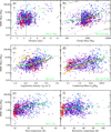 |
Fig. 7 Same as Figure 4, but for the MMC mass along the y-axis of each panel. The symbol under each panel represents the typical error bar associated with the data. The dotted gray lines in panel b indicate the trends for constant fMMC values. In panel c, the solid gray line indicates the power-law fit to the data, and the open yellow triangles represent data from Morii et al. (2023). In panel d, the gray line represents the median mass of the least massive core in each clump. |
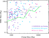 |
Fig. 8 Mass of the MMC vs. clump mass for ALMAGAL (open blue diamonds) and CORNISH (South) (light blue-filled circles) star-forming targets, limited to 8 × 10² M⊙ < M < 2 × 10⁴ M⊙ and 1 × 10⁴ L⊙ < L < 6 × 10⁵ L⊙. The green line connects the medians of MMC mass in logarithmic bins of 0.2 for the entire sample (as in Figure 7, panel b), while the gray line is recalculated only with the points plotted here. Furthermore, magenta-filled squares represent the values by Xu et al. (2024a). |
4.3 Mass of the most massive core versus evolutionary status
Before exploring the behavior of MMMC as a function of specific evolutionary parameters, we show in Figure 9 the distributions of MMMC separated by evolutionary class. While the top panel shows the distributions as histograms along with their respective medians, the bottom panel presents the corresponding cumulative distributions, which highlight the differences between the subclasses.
A systematic shift toward higher values in the median and interquartile ranges is observed (see also Table 2). In particular, the MMC masses in clumps associated with radio counterparts are higher than those in quiescent clumps. Specifically, the average masses for these two subclasses are 5.1 M⊙ (average: 17.4 M⊙) and 0.9 M⊙ (average: 1.8 M⊙), respectively. However, these distributions appear broad, with significant overlap among the classes, making it difficult to define distinct ranges of MMMC for each evolutionary category.
What is clear is that, on the one hand, not all evolved ALMAGAL targets host at least one candidate core capable of forming a massive star (i.e., with a mass of at least 24 M⊙) and, on the other hand, such cores are entirely absent in clumps classified as quiescent. This suggests that the masses of massive cores are not definitely established during the earliest phases of fragmentation (see also below).
Based solely on continuum ALMA photometry, we cannot in turn distinguish between the quiescent and star-forming nature of these massive cores when observed. Further confirmation from ALMAGAL line observations (e.g., Jones et al., in prep.; Benedettini et al., in prep.; Allande et al., in prep.) is required to determine whether these are massive prestellar cores (Xu et al. 2024a, and references therein), or if all of them already host active star formation.
When examining the relationships between the MMC mass and clump evolutionary parameters, an increasing trend is observed in the median MMMC in bins of clump L/M and temperature (Figure 7, panels d and e, respectively), while a possible similar trend for the bolometric temperature is hard to see (panel f). Coletta et al. (2025) already commented on the relation with L/M, highlighting that it is all the more appreciable if compared with the flat trend of the minimum core mass found in the clump. This suggests that the mass of the MMC is not determined at the earliest phases of the clump evolution (as supposed, for example, by Anderson et al. 2021, for clumps coincident with hubs of filaments) but the MMC increases in mass with the advancement of the evolutionary stage. At the same time, the formation of cores of smaller mass is not inhibited (cf. Pillai et al. 2019).
The observations show that the minimum L/M where MMMC > 24 M⊙ occurs at ~1 L⊙/M⊙. We observe no quiescent clumps with cores exceeding this mass (similarly to what was found by Sanhueza et al. 2019; Morii et al. 2023; Cheng et al. 2024). This indicates that many quiescent Herschel clumps, though meeting the necessary (but not sufficient) conditions in surface density for massive star formation (Elia et al. 2021), are unlikely to host massive cores at the current evolutionary stage. Furthermore, Baldeschi et al. (2017) highlighted the potential for misclassifications of such clumps due to distance-related biases.
These findings imply three possible scenarios. In the first one, quiescent clumps capable of forming massive cores evolve so rapidly that this phase becomes practically elusive, or core masses increase over time, as suggested by the trend in panel d. In the second scenario, newly formed cores are initially insufficiently massive to form high-mass stars but grow through continued accretion, which is consistent with the competitive accretion model (Bonnell et al. 2004; Wang et al. 2010). This hypothesis, previously put forward by Sanhueza et al. (2017, 2019), Morii et al. (2021, 2023, 2024), and Li et al. (2023), is here reinforced with a much broader statistical foundation. A third possibility, proposed within the GHC framework by Vázquez-Semadeni et al. (2019), suggests that the earliest fragments to collapse are the most extreme local density fluctuations, with low total masses, and as the mean density of the environment increases, more massive fragments also reach the conditions necessary for collapse.
The relationship between MMC mass and dust temperature is qualitatively similar to the relationship with L/M, while, as noticed above, the link with bolometric temperature looks much weaker. It appears that, as with L/M, the highest MMC mass values occur before the right tail of the highest values of these indicators. This suggests that for the ALMAGAL targets in the most advanced stages, the MMC might be entering the envelope cleaning-up phase, potentially driven by one or more newly formed high-mass stars.
To assess whether the MMC mass is influenced by the fact that the MMC is isolated or, conversely, lies in a cluster with multiple companions, Figure 10 displays the MMC mass against Ncore. While the highest MMC masses (MMMC > 10 M⊙) are observed across a wide range of fragmentation levels, appearing largely insensitive to it, the lower envelope of the MMC mass distribution shows a clear trend of increasing with Ncore. In particular, MMC masses below 1 M⊙ are almost entirely absent for Ncore ≳ 25.
To summarize this evidence, the mass of the MMC within a clump tends, on average, to increase as the core population becomes more numerous, consistent with the basic trend predicted by the competitive accretion Bonnell et al. (2004); Wang et al. (2010) and GHC (Vázquez-Semadeni et al. 2019) scenarios. However, we note that an inverse correlation, albeit based on a significantly smaller statistical sample, has been reported by Pandian et al. (2024).
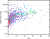 |
Fig. 10 Mass of the MMC versus the level of fragmentation for ALMAGAL targets. The symbol and color-coding used for source subclasses is the same as in Figure 4 and throughout the paper. The green line represents the median in bins of ΔNcore = 2. |
4.4 Maximum core mass versus bolometric luminosity
The analysis of the relationship between MMC mass and the L/M ratio in panel d of Figure 7 underscores the importance of investigating whether the increase in core mass is specifically linked to the bolometric luminosity L. Our aim is to ascertain whether the growth in the mass of the MMC within the clump, potentially indicative of a forming star, significantly drives the overall rise in clump luminosity. It is noteworthy that both parameters exhibit the same analytical dependence on distance.
For this purpose, we build Figure 11 based on the following logic: first, we checked whether an increased number of fragments can produce, in general, an increment of L. This is not necessarily expected, as Ncore can increase due to the fragmentation of larger condensations into smaller and fainter ones. In fact, Palau et al. (2013) find no apparent correlation between these quantities in a sample of 18 objects. At this point, we assessed whether the MMC mass can produce an increment of L and whether a similar behavior can be identified for the total mass of cores.
In the top-left panel of Figure 11, we see that high luminosities (L > 104 L⊙) are found throughout the entire range of Ncore. In contrast, the lowest ones tend to increase with Ncore, so that in the presence of a large number of fragments (say Ncore > 30), only high luminosities (say L > 104 L⊙) are found.
The top-right panel of Figure 11 illustrates the L versus MMMC relation. A clear increasing trend is observed in the median of L, approximable by a power-law behavior, with even more distinct trends evident for the quiescent and HII region counterparts. Performing a linear fit to the logarithms of the data yields an exponent 0.8 (approximately three times shallower than that found in Pandian et al. 2024); the Spearman’s coefficient is ρS = 0.47. To assess whether this trend arises solely from the distance effect spreading L and MMMC along a linear relation, the bottom-left panel of Figure 11 plots these quantities normalized by the distance, namely L/d2 versus MMMC/d2. After normalization, the correlation seen in the top-right panel survives, with a power-law slope 0.7 and a Spearman’s coefficient ρS = 0.45. In conclusion, while a correlation between the lower luminosity limit and the level of fragmentation is apparent, a mild physical correlation between luminosity and MMC mass is identified, which is not significantly affected by the distance effect. Using the total mass in cores instead of the MMC mass (Figure 11, bottom-right panel) yields a result qualitatively similar to that with MMC mass, with the median luminosity showing a nearly linear increase.
5 Core formation efficiency
Another parameter used to quantify the fragmentation of a clump is the CFE, defined as the total mass of the cores identified in a clump divided by the clump’s total mass. In this case, we adopted the clump mass estimate from Elia et al. (2017), although in principle, the mass should be determined before fragmentation begins, since the clump could accrete further mass from the parental cloud or lose mass due to star formation activity. Moreover, as seen above and further elaborated in this section, the mass contained in the cores evolves over time, making it more accurate to refer to the “instantaneous” CFE. Therefore, hereafter we use the term CFE implicitly implying its instantaneous value.
Based on this definition, the derived CFEs range from 0.01% to 15%, with a median of 0.4%. Comparing these results to Anderson et al. (2021), who report a maximum CFE of 33%, a minimum of 12%, and a median of 24%, and Morii et al. (2023), who report a maximum of 16%, a minimum of 0.6%, and a median of 4.4%, respectively, reveals a distinctly different regime of values. This discrepancy arises primarily from differences in observational resolution, source extraction strategy, and assumptions in converting photometry to masses.
First, the dust opacity values used by Elia et al. (2017, 2021) and Coletta et al. (2025) to derive clump and core masses, respectively, differ to account for the distinct characteristics of these two environments. As noted in Sect. 2, assuming the same gas-to-dust ratio, Elia et al. (2017, 2021) adopt 0.9 cm2 g−1 at 1.3 mm, whereas Coletta et al. (2025) adopt 10 cm2 g−1 at 300 μm with a dust emissivity exponent β = 2, which scales to ~0.53 cm2 g−1 at 1.3 mm – a factor of 1.7 lower than in Coletta et al. (2025). Consequently, adopting the same value for both would roughly double the core masses or halve the clump masses, significantly increasing the CFE.
Furthermore, the higher angular resolution of the ALMAGAL images may result in worse brightness sensitivity, potentially hindering the detection of fainter and extended structures. Structures lacking prominent peaks may remain undetected when angular resolution improves, as also seen in ALMAGAL when transitioning from 7M+TM2 to 7M+TM2+TM1 maps (Sánchez-Monge et al. 2025; Coletta et al. 2025). In contrast, in the ASHES survey8, such objects can be detected and cataloged, contributing to a higher number of fragments and, consequently, a higher total mass in cores (cf., e.g., Merello et al. 2015). Additionally, a higher number of cores in ASHES can be surely due to the larger field coverage, as their maps are mosaics obtained from ten pointings. This difference can be checked in the ten overlapping fields between ALMAGAL and ASHES, where fragment counts vary from 0 to 9 in ALMAGAL (with CFE < 1% in all cases) but from 9 to 39 in ASHES (with 0.6 < CFE < 16.4%, Morii et al. 2023). Additionally, the ALMAGAL photometry extraction strategy includes selecting compact sources and subtracting background emission (Sect. 2.2), which results in lower flux estimates compared to algorithms such as Astrodendro (Robitaille et al. 2019). Using background emission values from Coletta et al. (2025), unsubtracted ALMAGAL fluxes are estimated to be, on average, twice as large. Furthermore, Morii et al. (2023) use a temperature of 13.8 K to derive core masses, while ALMAGAL adopts a temperature of 20 K or higher (Section 2.2), resulting in at least 40% lower mass. Lastly, unlike ASHES mosaics, the relatively smaller FOV of ALMAGAL single-pointing maps for the largest clumps may exclude fragments at the edges, underestimating the CFE. However, it is to say that, as shown in the top panel of Figure 12, most clumps have circularized sizes under 35″, i.e., within the ALMAGAL FOV. A decrease in CFE with the clump size (diameter) is observed (Figure 12, top), while no strong link to clump mass is found (Figure 12, bottom), because the mass also depends on surface density and heliocentric distances, and because of the lower cut adopted on clump masses for selecting most of the ALMAGAL sample (Sect. 2.1).
Finally, before examining the relationships between the CFE and clump parameters, it is important to consider the connection between the CFE and the MMMC (Figure 13, top). One might argue that the two quantities are correlated and that discussing both constitutes a circular argument. However, although the mass of the MMC contributes to the numerator in the definition of CFE, much can depend on the contribution from the other cores. Moreover, CFE also depends on the clump mass in the denominator and is distance-independent, unlike MMMC. Nevertheless, the figure reveals a clear, steadily increasing trend, possibly indicating that the presence of a more massive core leads to a higher CFE, irrespective of the total clump mass. This implies that having at least one higher-mass core is associated with increased efficiency in converting clump material into cores, with the MMC playing a primary role in this process. More likely, as discussed in Sect. 4.3 and as shown in Sect. 5.3, both quantities tend to increase as the clump evolves. In this respect, the trend observed in the upper panel of Figure 13 should primarily reflect an evolutionary effect.
To investigate this aspect, in the lower panel of Figure 13 we show the distributions (also in cumulative form) of the ratio between MMMC and the total core mass, excluding the trivial cases with Ncore = 0 or 1. Despite the observed spread, the distributions, even more clearly visible through the cumulative curves and median positions, shift toward lower values as the evolutionary stage of the clumps advances. This indicates that, although MMMCincreases on average with clump age, its relative contribution to the total mass in cores tends to decrease, both because the number of cores grows and because their individual masses also increase.
In conclusion, the correlation observed between MMMC and the CFE in the top of Figure 13 does not appear to be driven solely by the analytical relation between the two quantities, which is also influenced by other parameters. This justifies treating CFE as an independent parameter in the following analysis, exploring its dependence on the clump properties.
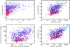 |
Fig. 11 Clump bolometric luminosity L plotted against the fragmentation level (top left), mass of the MMC (top right), mass of the MMC normalized by the square of the distance (with luminosity normalized as well, bottom left), and sum of core masses (bottom right). The symbol and color-coding used for source subclasses is the same as in Figure 4 and throughout the paper. In the top-right and bottom-right panels, the green line represents the median in bins of the quantity on the x-axis. |
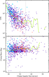 |
Fig. 12 Top: CFE against clump angular size, estimated from Herschel photometry at 250 μm. The symbols are defined as in Figure 4. The green line connects the median of the size estimated in bins of 2″. The vertical dotted line represents the diameter of the ALMAGAL FOV. Bottom: same as in the top panel, but for the clump mass on the y-axis. |
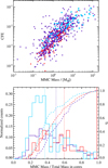 |
Fig. 13 Top: CFE against mass of the MMC (MMMC). Symbols are defined as in Figure 4. Bottom: distribution of the ratio between the mass of the MMC and the total mass contained in cores (excluding clumps with Ncore=0 or 1), shown separately for quiescent (red histogram), star forming (blue), and UCHII regions (cyan). The dashed curves represent the corresponding cumulative distributions, with values referenced to the y-axis on the right side of the plot. The vertical dotted lines mark the median values for each subclass, using the same color scheme as the histograms. |
5.1 CFE versus distance
A high degree of scatter is seen for CFE plotted against heliocentric distance in panel a of Figure 14. The median CFE is seen to slightly decrease with distance in the 2 kpc ≲ d ≲ 6 kpc range. The Spearman’s correlation coefficient for log(CFE) versus d is −0.16 within this distance range, and −0.24 for the entire sample, mildly supporting this trend. In the same distance interval, the level of fragmentation is also observed to decrease (Sect. 3.2). Therefore, also in this case, if one assumes that the observed trend is genuine, it can be interpreted in light of the progressive lack of low-mass cores that fall below the sensitivity limit as the distance increases.
The behavior of CFE of a region as a function of distance as a pure effect of virtually moving it away (so considering the distance bias due to lack of resolution, but not of sensitivity) was described by Baldeschi et al. (2017). They found a constant behavior for CFE at d ≳ 1.5 kpc, with average values varying from region to region in the range 1–20%, again generally higher than CFE we find for ALMAGAL clumps. Finally, we observe no evident break in the CFE behavior at the boundary separating the initial “near” and “far” ALMAGAL sample (d > 4.66 kpc). We conclude that the observed decrease in the median CFE is mostly attributable to the decrease in sensitivity with distance rather than of resolution.
5.2 CFE versus clump mass and density
As expected from Figure 12, the plot of the CFE and the clump mass M (Figure 14, panel b) does not show a correlation between the two; nevertheless, from the analytical point of view, M is present in both quantities. This means that the scatter in the total core mass (numerator of CFE) predominantly produces the observed large scatter of these two quantities.
A slightly more visible correlation, at least in terms of median values, is seen between the CFE and the clump surface density Σ (Figure 14, panel c). Again, the two quantities are inversely related from the analytical point of view (as both depend on the clump mass), so that, in this respect, the CFE should be expected to decrease at increasing mass, then increasing Σ. In contrast, in the ALMAGAL targets, the CFE increases, on average, with increasing Σ, i.e., these two quantities appear correlated in a way overpowering the underlying dependence on the mass. This means that other parameters at play, such as the core masses and the clump sizes, are crucial to establishing the observed behavior.
The mild (ρS = 0.29) increase in median CFE (as well as MMMC) with clump density, as also noted by Palau et al. (2013) and Csengeri et al. (2017), can suggest a growing importance of the role of gravity at increasing densities. If this evidence holds despite the scatter in the data, two alternative scenarios are conceivable. In one, an increased CFE can be interpreted as a consequence of high-density conditions. In the other, a high clump density might simply reflect a structure dominated by compact, dense substructures, and thus associated with a high CFE.
5.3 CFE versus evolutionary status
The distributions of the CFE for the three evolutionary classes of targets exhibit a progressive shift toward higher values from quiescent to star-forming clumps and then to UCHII regions, though with significant overlap (Figure 15, panel a, and Table 2). This is even clearer if shown in terms of cumulative distributions (Figure 15, panel b).
The increase in clump formation efficiency (i.e., the ratio of total mass in clumps to the mass of the containing cloud) as a result of feedback-induced triggering by HII regions has been proposed by Eden et al. (2013) and Xu et al. (2018). The higher median CFE observed for ALMAGAL targets associated with radio emission may suggest an extension of this mechanism to clump-to-core scales. Additionally, the pronounced left skewness in the Ncore distribution for these sources, compared to other classes (Figure 5), would support this interpretation. Also, Zhang et al. (2024) observe the presence of massive and dense cores around Hir regions, although the origin of their large masses remains unclear. However, the large spread in CFE values within this subclass (spanning more than two orders of magnitude) makes it difficult to generalize this scenario to all cases.
The behavior of the CFE as a function of the evolutionary stage can be also examined by means of panels d, e, and f of Figure 14. In all of them, the median CFE exhibits an increasing trend. In particular, the CFE versus L/M plot (panel d) shows a quite regular increase not only of the median CFE, but also of the highest values of the CFE in bins of L/M, whereas the lowest values of CFE (say <3 × 10⁻⁴) appear present practically at all L/M regimes. A power-law fit to the entire population of clumps gives a dependence of the form
![Mathematical equation: $\[\mathrm{CFE}=10^{-2.54 \pm 0.02}\left[\frac{L / M}{\mathrm{~L}_{\odot} / \mathrm{M}_{\odot}}\right]^{0.36 \pm 0.02},\]$](/articles/aa/full_html/2026/01/aa54764-25/aa54764-25-eq2.png) (2)
(2)
(parameter uncertainties are simply derived from least squares fitting to data). A similar behavior is also seen for the dust temperature (panel e):
![Mathematical equation: $\[\mathrm{CFE}=10^{-5.42 \pm 0.13}\left[\frac{T}{\mathrm{~K}}\right]^{2.5 \pm 0.1}.\]$](/articles/aa/full_html/2026/01/aa54764-25/aa54764-25-eq3.png) (3)
(3)
It is expected that the fraction of clump mass contained in cores increases with time (e.g., Chen & Ostriker 2015), under the effect of gradual accretion on cores and formation of further cores, unless this is eventually halted by feedback from the first newly formed stars. However, in the range of evolutionary stages covered by the ALMAGAL sample (up to a few 105 years), we do not see, on average, an evident flattening of the CFE trend against clump evolutionary parameters. The behavior of the CFE as a function of clump evolution, measured by the L/M ratio, can also be analyzed through comparison with numerical simulations (Sect. 6.2).
6 Discussion
6.1 Ranking correlations between two variables
In Sect. 4.2, the Spearman’s coefficient for the MMMC versus clump mass was discussed to provide a quantitative estimate of the possible correlation between the two. We systematically extend this analysis to all relations between clump and corresponding core population properties. In particular, we obtain coefficients ρS by considering the n = 840 ALMAGAL targets with all clump properties defined and Ncore ≥ 1.
Figure 16 contains the matrix of Spearman’s coefficients ρS for pairs of parameters: d, log M, log Σ, log(L/M), T, and Tbol along the x-direction, and Ncore, log MMMC, and log CFE along the y-axis. The matrix of coefficients collects and summarizes the considerations made in Sects. 3, 4, and 5. It can be immediately seen that none of the reported ρS approaches values corresponding to the highest degree of correlation (+1) or anticorrelation (-1), but the range of the coefficients remains between −0.25 and 0.62.
The quantities exhibiting the highest correlation are the surface density (logarithm), the luminosity/mass ratio (logarithm), and the temperature. In more detail, the largest ρS are found for the relations between Ncore, Σ, and T. Temperature and surface density are quantities most correlated with MMMC as well, but with an inverted role, and with a lower correlation degree in general. Finally, for the CFE, the highest correlation is found with T and then with L/M, namely the two evolutionary parameters for which, in fact, an analytical relation was tentatively expressed in Equations (3) and (2), respectively. Generally, T consistently shows a stronger correlation with core population parameters compared to L/M. The third evolutionary parameter considered, Tbol, instead, shows lower values of the ρS coefficient. The mass M has notably less influence on fragmentation indicators than the surface density Σ. Only when combined with MMMC, which shares the M dependence on the square of the distance, do we observe a stronger correlation. Finally, distance itself shows a weak correlation with all core properties.
A similar analysis was conducted by Traficante et al. (2023), but using Pearson coefficients, which specifically indicate the reliability of linear correlations. They found direct correlations between MMMC and Σ, as well as between the CFE and both L/M and Σ, but no significant correlation between Ncore and other quantities, nor between MMMC and L/M. However, a direct comparison with our data is not feasible, as here we use Spearman’s coefficients instead of Pearson coefficients to provide a more general assessment of monotonic trends. Additionally, our analysis is based on a much larger statistical sample, which carries implications discussed below.
To determine whether the obtained Spearman’s coefficients indicate a true correlation between the two physical quantities, rather than a mere apparent association, the Spearman’s test should be invoked. However, this test may have limitations when applied to datasets with a large number of degrees of freedom, which in our case is n − 2, where n = 840 is the number of plotted data points. With a large sample size, Spearman’s rank correlation coefficient can become overly sensitive, detecting statistically significant correlations that may be weak or practically unimportant. This arises because, with large n, even minor deviations from the null hypothesis (no correlation) may yield small p-values9, potentially leading to the so-called Type I errors, i.e., where trivial relationships are flagged as significant. However, in our case, this is not straightforward. First, the critical values for the Spearman’s distribution decrease as the number n of measurements increases. For instance, in a two-tailed test for a positive association at the 5% significance level, the critical value is 0.65 for n = 10, but decreases to 0.36 for n = 30, 0.20 for n = 100, and 0.07 for n = 840, respectively (for details on the calculation of the last value, see Appendix E). Second, we performed a resampling test by extracting 100 random subsamples of 30 data points (out of 840) for each pair of variables, calculating the Spearman’s coefficient for each subsample, and taking the median of these 100 values. The absolute deviations of these median coefficients from the original ones presented in Figure 11 are small, not exceeding 0.06 in the most extreme cases. However, the 95% confidence threshold is more stringent for n=30 than for n = 840, meaning that for the smaller sample size, only the coefficients for Σ, L/M, and T would exceed it and then be statistically significant.
In conclusion, the interpretation of Spearman’s test results depends heavily on the sample size. In this respect, it appears inappropriate to compare coefficients derived from samples of significantly different sizes (Sect. 4.2). Within the same sample, the coefficients remain useful for comparative rather than absolute analysis, as done in the first part of this section.
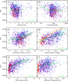 |
Fig. 14 Same as Figure 4, but for the CFE along the y-axis of each panel. In addition, in panels d and e, the gray solid lines represent the best power-law fit to data. |
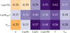 |
Fig. 16 Matrix of Spearman’s correlation coefficient ρS for relationships between clump physical parameters (x-axis) and core population parameters (y-axis). The color scale goes from dark orange (ρS = −1) to dark purple (ρS = 1) through white (ρS = 0). |
6.2 Multiparameter analysis
The analyses in Sects. 3, 4, and 5 focused on examining the relationship between a single overall descriptor of core populations and individual physical parameters of ALMAGAL targets, such as distance, mass, surface density, and evolutionary descriptors. This approach aimed to isolate the influence of each parameter on the observed characteristics of clump fragmentation. In this section, we take a step further by synthesizing those results and presenting them through multidimensional diagrams for a more comprehensive discussion.
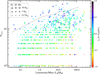 |
Fig. 17 Same as panel d of Figure 7, but with different symbols and color-coding. The color scale is coded according to the logarithm of the clump surface density in grams per square centimeter (color bar on the right), and quiescent clumps (SL in the legend in the top-left corner), star-forming ones (SF), and UCHII counterparts (HII) are displayed by means of open triangles, open diamonds, and filled circles, respectively. The symbol size scales as the logarithm of the mass of the MMC, as shown in the legend. The solid gray line represents the numerical prediction by Lebreuilly et al. (2025) with initial conditions set to M = 500 M⊙, ℳ = 7, and μ = 10, also plotted in panel e of Figure 7 as an orange line. |
6.2.1 Clump fragmentation level
In Figures 4, 7, and 14, we highlighted an increasing trend of Ncore, MMMC, and CFE parameters, respectively, both with increasing L/M, an evolutionary indicator, and Σ, which, as explained in Sect. 3.3 and Appendix A, is not univocally related to the evolutionary stage of the clump (and, consequently, to L/M). To better disentangle the interplay of these two parameters against clump fragmentation, in Figure 17 we show, similarly to panel e of Figure 4, an Ncore (here in logarithmic scale) versus L/M plot, but with symbol colors and sizes encoded according to Σ and MMMC, respectively.
We highlight again that the clearest trends observable in the Ncore versus L/M plot are the increase in the highest values of Ncore at increasing L/M, and the paucity of low fragmentation level (say Ncore < 10) in the (few) cases at L/M > 100 L⊙/M⊙. On the contrary, the correlation between Ncore and Σ appears to be tighter, as also testified by the Spearman’s coefficient analysis contained in Sect. 6.1.
The mass of the MMC appears correlated with L/M and Σ (more strictly with the latter, according to the quantitative analysis in Sect. 6.1). In particular, among the 31 clumps with MMMC > 24 M⊙ – compatible with the formation of a high-mass star – 30 have L/M > 1 L⊙/M⊙, a signature of ongoing star formation according to Molinari et al. (2016), and 24 have L/M > 10 L⊙/M⊙, which the same authors mostly attribute to the appearance of a first zero-age main-sequence star of intermediate or high mass. Among cases with L/M > 1 L⊙/M⊙, 22 of them show Σ > 1 g cm−2 (i.e., the theoretical threshold for compatibility with massive star formation of Krumholz & McKee 2008), while 27 fulfill the condition Σ > 0.5 g cm−2, which is a conservative value, higher than densities empirically found to be consistent with massive star formation (Tan et al. 2013; Urquhart et al. 2014; Traficante et al. 2018). On the contrary, no cores with mass exceeding 24 M⊙ are found in clumps with both L/M < 1 L⊙/M⊙ and Σ < 0.5 g cm−2.
Among the indications given by the plot in Figure 17, therefore, it emerges that the number of fragments is preferentially determined by density conditions in the clump, although Ncore can also increase with the clump evolution due to further fragmentation, or formation of new condensations (e.g., Zhang et al. 2015). Certainly, the growth of the fragment masses (or, at least, that of the most massive fragment) generally proceeds with the clump evolution, as would be expected for a clumpfed accretion scenario, and in particular by the GHC theory (Vázquez-Semadeni et al. 2019). As a further argument in favor of the clump-fed model over the core-fed one, we observe that (i) large-mass cores are not seen at early evolutionary stages, and (ii) isolated large-mass cores (corresponding to Ncore = 1 or 2) are not found at any evolutionary stage, as also shown in Figure 10. This means, indeed, that the mass reservoir available for the formation of a massive star is not set in the core before it collapses (as required by the core-fed model of McKee & Tan 2003), and also that the mass growth of such a core with time takes place in the presence of and in connection with other cores accreting mass from the same clump (Vázquez-Semadeni et al. 2019; Padoan et al. 2020), most likely in a competitive manner (Bonnell et al. 2001, 2004).
Of course, as discussed below, superposed on these overall trends are peculiar conditions in each clump – dictated by magnetic field, turbulence, and protostellar feedback – that can determine the observed fragmentation level and likely account for the high degree of scatter characterizing all plots from Figures 4 to 14. These factors cannot be quantified at this stage, i.e., by means of ALMAGAL continuum photometry alone, but rather need to be further characterized by ALMAGAL spectral line analysis (Jones et al., in prep.; Benedettini et al., in prep.). Finally, it has to be pointed out that, as highlighted in Sect. 3.2, the level of fragmentation is particularly sensitive to the core flux sensitivity limit in the ALMAGAL catalog, so that in principle the Ncore values plotted in various figures might be intended as lower limits for this quantity.
6.2.2 Comparison with simulations
We have the opportunity to compare the ALMAGAL data with predictions from numerical simulations, following an approach similar to that of Fontani et al. (2018). We use recent numerical simulations produced by the Rosetta Stone project (Lebreuilly et al. 2025), aimed at investigating the fragmentation of massive clumps (M ≥ 500 M⊙) and subsequent star formation10. The first step of this project consists of simulating the clump collapse (Lebreuilly et al. 2025) by using the RAMSES code (Teyssier 2002; Fromang et al. 2006) and its extension to radiative transfer in the flux-limited diffusion approximation (Commerçon et al. 2011, 2014). Lebreuilly et al. (2025) simulated the collapse of clumps with 500 and 1000 M⊙, exploring different regimes of turbulence and magnetization, and obtained predictions of fragmentation and star formation efficiency as a function of the clump evolutionary stage, represented by the L/M ratio. We consider, in particular, the case with the following combination of initial parameters, which best matches our data: initial clump size ~0.38 pc (total size of the cube ~1.5 pc), mass M = 500 M⊙, turbulent Mach number ℳ = 7, and mass-to-magnetic flux ratio (in units of the critical mass-to-flux ratio) μ = 10; finally, temperature T = 10 K, which is common to all models. Single forming stars are represented in these models by sink particles (Bleuler & Teyssier 2014) that form above a number density threshold of 109 cm−3. The maximum resolution, in terms of physical scale, from the adaptive mesh refinement is equivalent to ~400 au.
The predicted number of sink particles (gray line in Figure 17, and orange line in Figure 4 (panel d) exceeds most ALMAGAL values by a factor ≳2, though it follows a similar increasing trend to that of the highest values of Ncore. Other parameter combinations yield stronger fragmentation and poorer agreement, particularly for higher masses (1000 M⊙) or weaker fields (μ = 100). An anticorrelation between magnetic field and fragmentation degree was tentatively found in observations by, for example, Cortes et al. (2019), Añez-López et al. (2020), Palau et al. (2021), and Sanhueza et al. (2025). Therefore, an opposite scenario, i.e., a model with μ < 10, might be expected to better reproduce our data (for example, μ = 2 is suggested by Beuther et al. 2018b, based on observations). However, the simulations produced within the Rosetta Stone framework with μ = 3 have offered complementary insights into how strong magnetization influences fragmentation. Lebreuilly et al. (2025), who analyzed the number of sink particles with clump age, report that runs with μ = 3 yield fewer sink particles than those with μ = 10, whereas Nucara et al. (2025) in post-processed versions of the same simulations (at ~7000 au resolution) find that the μ = 3 and μ = 10 models are not clearly distinguishable in terms of their fragmentation properties, seen as a function of L/M. Post-processing of these simulations at the ALMAGAL resolution is among the next planned steps of the Rosetta Stone project and is expected to help resolve this apparent discrepancy.
Turbulence also plays a role: while it supports large-scale stability, it can enhance small-scale compression (Federrath & Klessen 2013). Observations indicate that higher turbulence favors massive core formation (Olmi et al. 2023), whereas simulations show that reducing Mach number increases fragmentation (Fontani et al. 2018); thus, values below ℳ = 7 may better fit ALMAGAL results.
Stellar feedback, not yet included in these simulations, can contribute to suppress fragmentation (Krumholz et al. 2007; Myers et al. 2013; Kruijssen et al. 2019; Hennebelle et al. 2020; Geen et al. 2023), although the relative contributions of these mechanisms remain a subject of active debate (e.g., Dale 2015; Hopkins et al. 2020). Consequently, it may help explain the observed discrepancy, especially in evolved fragments.
Observational biases must also be considered. The number of detected fragments depends on the adopted detection threshold (5 σ, Coletta et al. 2025), which undercounts faint cores. Moreover, while the simulations of Lebreuilly et al. (2025) track sink masses down to 0.001 M⊙, the observational catalog is complete only above 0.2 M⊙ Coletta et al. (2025), likely missing low-mass fragments. Finally, simulations treat sink particles as discrete entities that do not merge, even when in close proximity. In contrast, in the observations, limited angular resolution and projection effects can merge nearby sources, further lowering the observed Ncore.
The clump collapse simulation of Lebreuilly et al. (2025) also accounts for mass accretion onto sink particles (Figure 7, panel d, orange curve). In qualitative terms, the observed increasing trend of MMMC appears similar to that predicted by this model for the mass of the most massive sink particle.
6.2.3 Core formation efficiency
To further examine the CFE (Sect. 5), Figure 18 presents a view of its dependence on clump L/M and Σ (seen also by Pandian et al. 2024). As previously noted in Figure 14, the increasing trend of the CFE with L/M is more pronounced than the corresponding trend in Ncore shown in Figures 4 and 17, and is quantitatively confirmed in Figure 16. Although there is also a contextual increase in the CFE with Σ (cf. Könyves et al. 2015), Figure 16 indicates that this correlation is weaker compared to the CFE-L/M relationship. In other words, the scenario is opposite to what is seen for the number of fragments: compared with Ncore, the CFE appears, in general, more sensitive to the clump evolution than to surface density.
Furthermore, the CFE shows a strong correlation with MMMC, confirming the result of Traficante et al. (2023). The high values of both parameters are prominently found at L/M ≳ 10 L⊙/M⊙, with less regard for the value of Σ.
When examining this evidence in the context of discerning between theories of massive star formation, multiple arguments emerge against a core-fed scenario. In this model, cores appear as preassembled mass reservoirs; therefore, core masses and the CFE are not expected to increase significantly over time, which contrasts with our observations. If cores are prevented from further accreting mass from the clump, as in the core-fed scenario, those with a mass below a threshold to form massive stars would not fulfill that threshold with time, contrary to what is observed for the highest values of MMMC.
In contrast, our analysis suggests a more dynamic evolution of the core population within a clump. The number of cores appears to be primarily determined by the density of the clumps, while both CFE and the mass of the MMC (MMMC) show a more general and systematic increase as the system evolves. This trend indicates continuous accretion from the clump reservoir, supporting a clump-fed model rather than a static core-fed model (see also Contreras et al. 2018; Morii et al. 2024, and references therein). Furthermore, the fact that massive cores (MMMC > 24 M⊙) are only observed in targets where L/M ≳ 1 L⊙/M⊙ (Sect. 4.3) implies that massive star formation cannot be predicted solely from the physical parameters at the onset of clump collapse (as also shown by Klessen & Burkert 2000, 2001; Reid & Wilson 2005, 2006) and initial fragmentation. Instead, the evolution of core masses appears to be a time-dependent process, with sustained accretion playing a crucial role in the formation of massive stars. This conclusion gains further significance when considering that the ALMAGAL sample was specifically selected to represent conditions that are expected to be conducive to massive star formation.
A tentative comparison with model predictions can be carried out by displaying in the CFE versus L/M plot (Figures 14, panel d, and 18) the sink particle formation efficiency versus L/M curves emerging from the simulation of Lebreuilly et al. (2025) described above in this section. Remarkably, the behavior of these theoretical points is to increase at increasing L/M, as well as the median of ALMAGAL data.
Quantitatively speaking, the model prediction becomes definitely larger than the average of observational CFE for L/M > 0.3 L⊙/M⊙. The considerations to explain this discrepancy can be the same given for the Ncore versus L/M case (Sect. 3), such as the limitation imposed by sensitivity in detecting cores in observations, compared to the infinite sensitivity of simulations, as well as the absence of stellar feedback in the considered simulations.
In summary, the distribution of core masses in a clump appears to evolve over time, with cores dynamically gaining mass from their surrounding reservoir. This supports a clump-fed scenario of star formation, where the formation and growth of cores are closely related to the ongoing evolution and accretion processes within the clump. A similar conclusion for ALMAGAL is also reached by Coletta et al. (2025), based on the study of the temporal evolution of the core mass function.
7 Summary and conclusions
This paper investigates the fragmentation characteristics of clumps as described by their internal core populations, as observed in continuum maps at 1.4 mm of the ALMAGAL survey. Using data from an unprecedented sample of 1007 Galactic plane clumps observed by ALMA at high resolution, this study seeks to correlate fragmentation levels and core masses with the clump photometric and physical parameters. Our findings partially confirm earlier results in the literature but provide greater statistical reliability. Moreover, they uncover previously unexplored aspects of fragmentation.
The main results are:
The flux densities of the targets at Herschel wavelengths increase, on average, as a function of the number of hosted fragments (Ncore), particularly for 1 ≤ Ncore ≤ 25. The slope of this increase varies systematically with wavelength (decreasing from 70 to 500 μm), indicating a correlation between Ncore and clump temperature. Clumps without detected cores tend to have lower flux densities. These are typically less evolved or less dense compared to the whole ALMAGAL sample;
The ALMAGAL sample covers a broad range of clump properties (physical, evolutionary, and environmental conditions). This diversity leads to significant scatter in the relationships between these parameters and clump fragmentation descriptors. While continuum observations cannot directly quantify the roles of magnetic fields, turbulence, or protostellar feedback, in the future systematic comparisons with numerical simulations based on theoretical models will provide critical insights;
Although the data are widely scattered, average trends emerge. Fragmentation parameters – namely the number of fragments (Ncore), the mass of the MMC (MMMC), and the CFE – show an increasing trend with both clump surface density (Σ) and evolutionary indicators such as dust mean temperature (T), luminosity/mass ratio (L/M), and bolometric temperature (Tbol). Spearman’s coefficient analysis shows Ncore correlates most strongly with Σ, whereas MMMC and CFE align best with T. Therefore, the number of cores appears to be primarily determined by the density of the clumps, while CFE and MMMC show a more general and systematic increase as the system evolves. Power-law fits quantify relationships between CFE and L/M and T, yielding slopes 0.36 and 2.5, respectively;
In contrast, the fragmentation parameters show no clear dependence on clump mass or heliocentric distance, apart from a mild sensitivity-driven decrease in Ncore with distance;
Dividing the ALMAGAL targets into evolutionary classes (quiescent, SF, and UCHII regions), we observe a greater degree of segregation with respect to certain clump parameters, particularly those with evolutionary significance, compared to core population parameters. While the properties of core populations in SF clumps and UCHII regions appear somewhat intermixed, quiescent cores exhibit clear upper limits: Ncore < 20, MMMC < 8 M⊙, and CFE < 2%. The level of fragmentation and the distribution of CFE observed for UCHII regions may suggest a mechanism of core formation triggering;
When comparing the data with the currently available and debated star formation models, the strong dependence of MMMC and CFE on the clump evolution aligns more closely with the family of models categorized under the clump-fed scenario, indicating lower compatibility with the core-fed model.
Acknowledgements
The authors thank the anonymous referee for their constructive and engaged approach, which, with precise suggestions and insightful remarks, helped us improve the overall quality of this article. The teams at INAF-IAPS and at Heidelberg University acknowledge financial support from the European Research Council via the ERC Synergy Grant “ECOGAL” (project ID 855130). RSK furthermore thanks the German Ministry for Economic Affairs and Climate Action in project “MAINN” (funding ID 50OO2206). RSK also thanks the 2024/25 Class of Radcliffe Fellows for highly interesting and stimulating discussions. A.S-M. acknowledges support from the RyC2021-032892-I grant funded by MCIN/AEI/10.13039/501100011033 and by the European Union ’Next Generation EU’/PRTR, as well as the program Unidad de Excelencia María de Maezto CEZ2020-001058-M, and support from PID2023-144675NB-I00 (MCI-AEI-FEDER, UE). G.A.F. acknowledges support from the Collaborative Research Centre 956, funded by the Deutsche Forschungsgemeinschaft (DFG) project ID 184018867. G.A.F. also gratefully acknowledges the DFG for funding through SFB 1601 “Habitats of massive stars across cosmic time” (subproject B1) and from the University of Cologne and its Global Faculty programme. R.K. acknowledges financial support via the Heisenberg Research Grant funded by the Deutsche Forschungsgemeinschaft (DFG, German Research Foundation) under grant no. KU 2849/9, project no. 445783058. P.S. was partially supported by a Grant-in-Aid for Scientific Research (KAKENHI Number JP22H01271 and JP23H01221) of JSPS. C.B. gratefully acknowledges funding from the National Science Foundation under Award Nos. 2108938, 2206510, and CAREER 2145689, as well as from the National Aeronautics and Space Administration through the Astrophysics Data Analysis Program under Award “3-D MC: Mapping Circumnuclear Molecular Clouds from X-ray to Radio”, Grant No. 80NSSC22K1125. L.B. gratefully acknowledges support by the ANID BASAL project FB210003. Part of this research was carried out at the Jet Propulsion Laboratory, California Institute of Technology, under a contract with the National Aeronautics and Space Administration (80NM0018D0004).
References
- Añez-López, N., Busquet, G., Koch, P. M., et al. 2020, A&A, 644, A52 [NASA ADS] [CrossRef] [EDP Sciences] [Google Scholar]
- Aguirre, J. E., Ginsburg, A. G., Dunham, M. K., et al. 2011, ApJS, 192, 4 [Google Scholar]
- Anderson, M., Peretto, N., Ragan, S. E., et al. 2021, MNRAS, 508, 2964 [NASA ADS] [CrossRef] [Google Scholar]
- André, P., Men’shchikov, A., Bontemps, S., et al. 2010, A&A, 518, L102 [NASA ADS] [CrossRef] [EDP Sciences] [Google Scholar]
- Avison, A., Fuller, G. A., Frimpong, N. A., et al. 2023, MNRAS, 526, 2278 [Google Scholar]
- Baldeschi, A., Elia, D., Molinari, S., et al. 2017, MNRAS, 466, 3682 [NASA ADS] [CrossRef] [Google Scholar]
- Basu, S., Ciolek, G. E., Dapp, W. B., & Wurster, J. 2009, New A, 14, 483 [NASA ADS] [CrossRef] [Google Scholar]
- Beltrán, M. T., Padovani, M., Girart, J. M., et al. 2019, A&A, 630, A54 [Google Scholar]
- Bergin, E. A., & Tafalla, M. 2007, ARA&A, 45, 339 [Google Scholar]
- Beuther, H., Schilke, P., Menten, K. M., et al. 2002, ApJ, 566, 945 [Google Scholar]
- Beuther, H., Mottram, J. C., Ahmadi, A., et al. 2018a, A&A, 617, A100 [NASA ADS] [CrossRef] [EDP Sciences] [Google Scholar]
- Beuther, H., Soler, J. D., Vlemmings, W., et al. 2018b, A&A, 614, A64 [NASA ADS] [CrossRef] [EDP Sciences] [Google Scholar]
- Beuther, H., Gieser, C., Soler, J. D., et al. 2024, A&A, 682, A81 [NASA ADS] [CrossRef] [EDP Sciences] [Google Scholar]
- Bleuler, A., & Teyssier, R. 2014, MNRAS, 445, 4015 [Google Scholar]
- Bonnell, I. A., Bate, M. R., Clarke, C. J., & Pringle, J. E. 2001, MNRAS, 323, 785 [Google Scholar]
- Bonnell, I. A., Vine, S. G., & Bate, M. R. 2004, MNRAS, 349, 735 [Google Scholar]
- Cesaroni, R., Pestalozzi, M., Beltrán, M. T., et al. 2015, A&A, 579, A71 [NASA ADS] [CrossRef] [EDP Sciences] [Google Scholar]
- Chen, C.-Y., & Ostriker, E. C. 2015, ApJ, 810, 126 [Google Scholar]
- Cheng, Y., Lu, X., Sanhueza, P., et al. 2024, ApJ, 967, 56 [Google Scholar]
- Coletta, A., Molinari, S., Schisano, E., et al. 2025, A&A, 696, A151 [NASA ADS] [CrossRef] [EDP Sciences] [Google Scholar]
- Commerçon, B., Hennebelle, P., & Henning, T. 2011, ApJ, 742, L9 [CrossRef] [Google Scholar]
- Commerçon, B., Debout, V., & Teyssier, R. 2014, A&A, 563, A11 [NASA ADS] [CrossRef] [EDP Sciences] [Google Scholar]
- Contreras, Y., Sanhueza, P., Jackson, J. M., et al. 2018, ApJ, 861, 14 [Google Scholar]
- Cortes, P. C., Hull, C. L. H., Girart, J. M., et al. 2019, ApJ, 884, 48 [Google Scholar]
- Csengeri, T., Bontemps, S., Wyrowski, F., et al. 2017, A&A, 600, L10 [NASA ADS] [CrossRef] [EDP Sciences] [Google Scholar]
- Dale, J. E. 2015, New A Rev., 68, 1 [NASA ADS] [CrossRef] [Google Scholar]
- Dunham, M. M., Offner, S. S. R., Pineda, J. E., et al. 2016, ApJ, 823, 160 [NASA ADS] [CrossRef] [Google Scholar]
- Eden, D. J., Moore, T. J. T., Morgan, L. K., Thompson, M. A., & Urquhart, J. S. 2013, MNRAS, 431, 1587 [NASA ADS] [CrossRef] [Google Scholar]
- Egan, M. P., Price, S. D., Kraemer, K. E., et al. 2003, VizieR Online Data Catalog:, 5114, 0 [Google Scholar]
- Elia, D., & Pezzuto, S. 2016, MNRAS, 461, 1328 [Google Scholar]
- Elia, D., Molinari, S., Schisano, E., et al. 2017, MNRAS, 471, 100 [NASA ADS] [CrossRef] [Google Scholar]
- Elia, D., Merello, M., Molinari, S., et al. 2021, MNRAS, 504, 2742 [NASA ADS] [CrossRef] [Google Scholar]
- Elmegreen, B. G. 2002, ApJ, 564, 773 [NASA ADS] [CrossRef] [Google Scholar]
- Federrath, C., & Klessen, R. S. 2013, ApJ, 763, 51 [Google Scholar]
- Fedriani, R., Tan, J. C., Telkamp, Z., et al. 2023, ApJ, 942, 7 [NASA ADS] [CrossRef] [Google Scholar]
- Fontani, F., Commerçon, B., Giannetti, A., et al. 2016, A&A, 593, L14 [NASA ADS] [CrossRef] [EDP Sciences] [Google Scholar]
- Fontani, F., Commerçon, B., Giannetti, A., et al. 2018, A&A, 615, A94 [NASA ADS] [CrossRef] [EDP Sciences] [Google Scholar]
- Fromang, S., Hennebelle, P., & Teyssier, R. 2006, A&A, 457, 371 [NASA ADS] [CrossRef] [EDP Sciences] [Google Scholar]
- Geen, S., Agrawal, P., Crowther, P. A., et al. 2023, PASP, 135, 021001 [NASA ADS] [CrossRef] [Google Scholar]
- Giannetti, A., Brand, J., Sánchez-Monge, Á., et al. 2013, A&A, 556, A16 [NASA ADS] [CrossRef] [EDP Sciences] [Google Scholar]
- Gómez, G. C., Vázquez-Semadeni, E., & Palau, A. 2021, MNRAS, 502, 4963 [CrossRef] [Google Scholar]
- Griffin, M. J., Abergel, A., Abreu, A., et al. 2010, A&A, 518, L3 [EDP Sciences] [Google Scholar]
- Guszejnov, D., Hopkins, P. F., & Krumholz, M. R. 2017, MNRAS, 468, 4093 [CrossRef] [Google Scholar]
- Gutermuth, R. A., & Heyer, M. 2015, AJ, 149, 64 [Google Scholar]
- Hennebelle, P., Commerçon, B., Joos, M., et al. 2011, A&A, 528, A72 [NASA ADS] [CrossRef] [Google Scholar]
- Hennebelle, P., Commerçon, B., Lee, Y.-N., & Chabrier, G. 2020, ApJ, 904, 194 [NASA ADS] [CrossRef] [Google Scholar]
- Hildebrand, R. H. 1983, QJRAS, 24, 267 [NASA ADS] [Google Scholar]
- Hopkins, P. F., GrudiĀ, M. Y., Wetzel, A., et al. 2020, MNRAS, 491, 3702 [CrossRef] [Google Scholar]
- Irabor, T., Hoare, M. G., Burton, M., et al. 2023, MNRAS, 520, 1073 [NASA ADS] [CrossRef] [Google Scholar]
- Ishihara, K., Sanhueza, P., Nakamura, F., et al. 2024, ApJ, 974, 95 [NASA ADS] [CrossRef] [Google Scholar]
- Kauffmann, J., & Pillai, T. 2010, ApJ, 723, L7 [Google Scholar]
- Kirk, H., Johnstone, D., Di Francesco, J., et al. 2016, ApJ, 821, 98 [Google Scholar]
- Klessen, R. S. 2001, ApJ, 556, 837 [NASA ADS] [CrossRef] [Google Scholar]
- Klessen, R. S., & Burkert, A. 2000, ApJS, 128, 287 [NASA ADS] [CrossRef] [Google Scholar]
- Klessen, R. S., & Burkert, A. 2001, ApJ, 549, 386 [Google Scholar]
- Könyves, V., André, P., Men’shchikov, A., et al. 2015, A&A, 584, A91 [Google Scholar]
- Kruijssen, J. M. D., Schruba, A., Chevance, M., et al. 2019, Nature, 569, 519 [NASA ADS] [CrossRef] [Google Scholar]
- Krumholz, M. R., & McKee, C. F. 2008, Nature, 451, 1082 [Google Scholar]
- Krumholz, M. R., Klein, R. I., & McKee, C. F. 2007, ApJ, 656, 959 [NASA ADS] [CrossRef] [Google Scholar]
- Krumholz, M. R., Cunningham, A. J., Klein, R. I., & McKee, C. F. 2010, ApJ, 713, 1120 [Google Scholar]
- Kumar, M. S. N., Palmeirim, P., Arzoumanian, D., & Inutsuka, S. I. 2020, A&A, 642, A87 [EDP Sciences] [Google Scholar]
- Lebreuilly, U., Traficante, A., Nucara, A., et al. 2025, A&A, 701, A217 [NASA ADS] [CrossRef] [EDP Sciences] [Google Scholar]
- Li, S., Sanhueza, P., Zhang, Q., et al. 2023, ApJ, 949, 109 [NASA ADS] [CrossRef] [Google Scholar]
- Lin, Y., Csengeri, T., Wyrowski, F., et al. 2019, A&A, 631, A72 [NASA ADS] [CrossRef] [EDP Sciences] [Google Scholar]
- Liu, T., Evans, N. J., Kim, K.-T., et al. 2020, MNRAS, 496, 2790 [Google Scholar]
- Liu, X., Liu, T., Zhu, L., et al. 2024, Res. Astron. Astrophys., 24, 025009 [CrossRef] [Google Scholar]
- Lumsden, S. L., Hoare, M. G., Urquhart, J. S., et al. 2013, ApJS, 208, 11 [Google Scholar]
- McKee, C. F., & Tan, J. C. 2002, Nature, 416, 59 [CrossRef] [Google Scholar]
- McKee, C. F., & Tan, J. C. 2003, ApJ, 585, 850 [Google Scholar]
- Mège, P., Russeil, D., Zavagno, A., et al. 2021, A&A, 646, A74 [NASA ADS] [CrossRef] [EDP Sciences] [Google Scholar]
- Menon, S. H., Lancaster, L., Burkhart, B., et al. 2024, ApJ, 967, L28 [NASA ADS] [CrossRef] [Google Scholar]
- Merello, M., Evans, II, N. J., Shirley, Y. L., et al. 2015, ApJS, 218, 1 [Google Scholar]
- Molinari, S., Pezzuto, S., Cesaroni, R., et al. 2008, A&A, 481, 345 [NASA ADS] [CrossRef] [EDP Sciences] [Google Scholar]
- Molinari, S., Swinyard, B., Bally, J., et al. 2010, PASP, 122, 314 [Google Scholar]
- Molinari, S., Schisano, E., Faustini, F., et al. 2011, A&A, 530, A133 [NASA ADS] [CrossRef] [EDP Sciences] [Google Scholar]
- Molinari, S., Merello, M., Elia, D., et al. 2016, ApJ, 826, L8 [Google Scholar]
- Molinari, S., Schilke, P., Battersby, C., et al. 2025, A&A, 696, A149 [NASA ADS] [CrossRef] [EDP Sciences] [Google Scholar]
- Morii, K., Sanhueza, P., Nakamura, F., et al. 2021, ApJ, 923, 147 [NASA ADS] [CrossRef] [Google Scholar]
- Morii, K., Sanhueza, P., Nakamura, F., et al. 2023, ApJ, 950, 148 [NASA ADS] [CrossRef] [Google Scholar]
- Morii, K., Sanhueza, P., Zhang, Q., et al. 2024, ApJ, 966, 171 [Google Scholar]
- Motte, F., Bontemps, S., & Louvet, F. 2018, ARA&A, 56, 41 [Google Scholar]
- Motte, F., Bontemps, S., Csengeri, T., et al. 2022, A&A, 662, A8 [NASA ADS] [CrossRef] [EDP Sciences] [Google Scholar]
- Myers, P. C., & Ladd, E. F. 1993, ApJ, 413, L47 [NASA ADS] [CrossRef] [Google Scholar]
- Myers, A. T., McKee, C. F., Cunningham, A. J., Klein, R. I., & Krumholz, M. R. 2013, ApJ, 766, 97 [Google Scholar]
- Nakamura, F., & Li, Z.-Y. 2005, ApJ, 631, 411 [NASA ADS] [CrossRef] [Google Scholar]
- Nucara, A., Traficante, A., Lebreuilly, U., et al. 2025, A&A, 701, A219 [NASA ADS] [CrossRef] [EDP Sciences] [Google Scholar]
- Olmi, L., Brand, J., & Elia, D. 2023, MNRAS, 518, 1917 [Google Scholar]
- Ossenkopf, V., & Henning, T. 1994, A&A, 291, 943 [NASA ADS] [Google Scholar]
- Padoan, P., Pan, L., Juvela, M., Haugbølle, T., & Nordlund, Å. 2020, ApJ, 900, 82 [NASA ADS] [CrossRef] [Google Scholar]
- Palau, A., Fuente, A., Girart, J. M., et al. 2013, ApJ, 762, 120 [NASA ADS] [CrossRef] [Google Scholar]
- Palau, A., Zhang, Q., Girart, J. M., et al. 2021, ApJ, 912, 159 [NASA ADS] [CrossRef] [Google Scholar]
- Pandian, J. D., Chatterjee, R., Csengeri, T., et al. 2024, ApJ, 966, 54 [Google Scholar]
- Pilbratt, G. L., Riedinger, J. R., Passvogel, T., et al. 2010, A&A, 518, L1 [NASA ADS] [CrossRef] [EDP Sciences] [Google Scholar]
- Pillai, T., Kauffmann, J., Zhang, Q., et al. 2019, A&A, 622, A54 [NASA ADS] [CrossRef] [EDP Sciences] [Google Scholar]
- Poglitsch, A., Waelkens, C., Geis, N., et al. 2010, A&A, 518, L2 [NASA ADS] [CrossRef] [EDP Sciences] [Google Scholar]
- Purcell, C. R., Hoare, M. G., Cotton, W. D., et al. 2013, ApJS, 205, 1 [Google Scholar]
- Ramsey, P. H. 1989, J. Educ. Statist., 14, 245 [Google Scholar]
- Reid, M. A., & Wilson, C. D. 2005, ApJ, 625, 891 [Google Scholar]
- Reid, M. A., & Wilson, C. D. 2006, ApJ, 644, 990 [Google Scholar]
- Rigby, A. J., Peretto, N., Anderson, M., et al. 2024, MNRAS, 528, 1172 [NASA ADS] [CrossRef] [Google Scholar]
- Robitaille, T., Rice, T., Beaumont, C., et al. 2019, astrodendro: Astronomical data dendrogram creator, Astrophysics Source Code Library [record ascl:1907.016] [Google Scholar]
- Rohatgi, V., & Saleh, A. 2015, An Introduction to Probability and Statistics, Wiley Series in Probability and Statistics (Wiley) [Google Scholar]
- Rosolowsky, E., Dunham, M. K., Ginsburg, A., et al. 2010, ApJS, 188, 123 [Google Scholar]
- Sánchez-Monge, Á., Brogan, C. L., Hunter, T. R., et al. 2025, A&A, 696, A150 [Google Scholar]
- Sanhueza, P., Jackson, J. M., Zhang, Q., et al. 2017, ApJ, 841, 97 [Google Scholar]
- Sanhueza, P., Contreras, Y., Wu, B., et al. 2019, ApJ, 886, 102 [Google Scholar]
- Sanhueza, P., Liu, J., Morii, K., et al. 2025, ApJ, 980, 87 [Google Scholar]
- Schisano, E., Molinari, S., Coletta, A., et al. 2025, A&A, submitted, arXiv e-prints [arXiv:2512.05914] [Google Scholar]
- Schuller, F., Menten, K. M., Contreras, Y., et al. 2009, A&A, 504, 415 [NASA ADS] [CrossRef] [EDP Sciences] [Google Scholar]
- Smith, J. D., Jaffa, S. E., & Krause, M. G. H. 2023, MNRAS, 525, 6182 [Google Scholar]
- Smith, M. D. 2014, MNRAS, 438, 1051 [NASA ADS] [CrossRef] [Google Scholar]
- Svoboda, B. E., Shirley, Y. L., Traficante, A., et al. 2019, ApJ, 886, 36 [Google Scholar]
- Tan, J. C., Kong, S., Butler, M. J., Caselli, P., & Fontani, F. 2013, ApJ, 779, 96 [Google Scholar]
- Tan, J. C., Beltrán, M. T., Caselli, P., et al. 2014, in Protostars and Planets VI, eds. H. Beuther, R. S. Klessen, C. P. Dullemond, & T. Henning, 149 [Google Scholar]
- Teyssier, R. 2002, A&A, 385, 337 [CrossRef] [EDP Sciences] [Google Scholar]
- Tokuda, K., Harada, N., Tanaka, K. E. I., et al. 2023, ApJ, 955, 52 [NASA ADS] [CrossRef] [Google Scholar]
- Traficante, A., Calzoletti, L., Veneziani, M., et al. 2011, MNRAS, 416, 2932 [Google Scholar]
- Traficante, A., Duarte-Cabral, A., Elia, D., et al. 2018, MNRAS, 477, 2220 [NASA ADS] [CrossRef] [Google Scholar]
- Traficante, A., Jones, B. M., Avison, A., et al. 2023, MNRAS, 520, 2306 [NASA ADS] [CrossRef] [Google Scholar]
- Urquhart, J. S., Thompson, M. A., Moore, T. J. T., et al. 2013, MNRAS, 435, 400 [Google Scholar]
- Urquhart, J. S., Moore, T. J. T., Csengeri, T., et al. 2014, MNRAS, 443, 1555 [Google Scholar]
- Urquhart, J. S., König, C., Giannetti, A., et al. 2018, MNRAS, 473, 1059 [Google Scholar]
- Vázquez-Semadeni, E., Palau, A., Ballesteros-Paredes, J., Gómez, G. C., & Zamora-Avilés, M. 2019, MNRAS, 490, 3061 [Google Scholar]
- Wang, P., Li, Z.-Y., Abel, T., & Nakamura, F. 2010, ApJ, 709, 27 [NASA ADS] [CrossRef] [Google Scholar]
- Wang, K., Zhang, Q., Testi, L., et al. 2014, MNRAS, 439, 3275 [Google Scholar]
- Wright, E. L., Eisenhardt, P. R. M., Mainzer, A. K., et al. 2010, AJ, 140, 1868 [Google Scholar]
- Xu, J.-L., Xu, Y., Zhang, C.-P., et al. 2018, A&A, 609, A43 [NASA ADS] [CrossRef] [EDP Sciences] [Google Scholar]
- Xu, F., Wang, K., Liu, T., et al. 2024a, ApJS, 270, 9 [NASA ADS] [CrossRef] [Google Scholar]
- Xu, F., Wang, K., Liu, T., et al. 2024b, Res. Astron. Astrophys., 24, 065011 [Google Scholar]
- Zar, J. 1999, Biostatistical Analysis, Prentice-Hall international edn. (Prentice Hall) [Google Scholar]
- Zhang, Q., Wang, Y., Pillai, T., & Rathborne, J. 2009, ApJ, 696, 268 [Google Scholar]
- Zhang, Q., Wang, K., Lu, X., & Jiménez-Serra, I. 2015, ApJ, 804, 141 [Google Scholar]
- Zhang, S., Liu, T., Wang, K., et al. 2024, MNRAS, 535, 1364 [Google Scholar]
Herschel (Pilbratt et al. 2010) is an ESA space observatory with important participation from NASA. Its onboard cameras for photometric observations include PACS (Poglitsch et al. 2010) and SPIRE (Griffin et al. 2010).
In this article, we use the terms fragment and core interchangeably to indicate the compact sources detected in such images, with a subtle distinction: fragment denotes the object as it appears in observations and is identified by the detection algorithm, while core emphasizes its physical nature.
In Figure 4, both the medians and averages of Ncore are presented as functions of various clump parameters to appreciate the differences between the two. However, the trends seen across all panels appear qualitatively similar, making it redundant to analyze the two values. Therefore, the discussion hereafter focuses solely on the behavior of the medians.
We note that even when showing the median trend with respect to the surface density calculated from deconvolved sizes (dotted black line in panel c of Figure 4, which is generally higher (see Section 2.1), the behavior does not change qualitatively, and all considerations discussed so far remain valid. The same also applies to the trends of the mass of the MMC (Sect. 4.2) and the CFE (Sect. 5.2), which we do not revisit in detail.
All medians reported in this paragraph are calculated excluding the cases in which Ncore = 0. Results including Ncore = 0 are also provided in Table 2.
For the UCHII regions, only one target appears to lack cores, so this subsample is excluded from the present discussion.
For a plot of all core masses as a function of the heliocentric distance, see Coletta et al. (2025).
Although the resolution is 5 to 10 times worse than in ALMAGAL, these images have better brightness sensitivity, enabling the detection of faint and extended structures. Such structures may potentially be detected in the 7M+TM2 ALMAGAL images (Coletta et al., in prep.).
The p-value represents the probability of obtaining a Spearman’s correlation coefficient at least as extreme as the one observed, assuming that there is no true correlation (the null hypothesis) between the variables.
An accurate comparison between models and observations requires post-processing of 3D simulations with radiative transfer to produce synthetic observations. Such work is currently underway within the Rosetta Stone project (Lebreuilly et al. 2025; Nucara et al. 2025). Accordingly, here we limit our discussion to general trends by directly comparing data and simulations, while noting caveats. Nucara et al. (2025) also provide a more systematic exploration of the simulation parameter space.
Appendix A Comparison of ALMAGAL target physical parameters
This appendix complements the review of clump physical properties given in Sect. 2, showing relations and concepts that are useful for the discussion in the main paper.
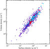 |
Fig. A.1 Volume density vs. surface density relation for ALMAGAL targets. The colors and symbols are the same as in Figure 4. |
First, we use Figure A.1 to motivate our choice of discussing surface density Σ throughout this paper, rather than using a volume density ρ, which could be estimated as the ratio of mass and volume of the sphere with the diameter equal to the circularized (not beam-deconvolved) source size at 250 μm. In the figure, in most cases, the two quantities appear directly correlated, making it quite redundant to consider these two quantities separately.
Another aspect we address here is the relation between the surface density of ALMAGAL targets and their evolutionary stage, expressed by the L/M ratio. A mild general increase in density from the starless to the star-forming phase was highlighted in Elia et al. (2017), and summarized in Sect. 3.3 of this paper. However, the high-pass filter selection criteria applied to both mass and surface density when selecting ALMAGAL targets from the Hi-GAL catalog (Molinari et al. 2025) prevent this trend from being observed within the ALMAGAL sample itself, as seen in Figure A.2 in terms of the Σ versus L/M relation.
A relevant consequence for our analysis is that any trends identified for a given fragmentation parameter as a function of these two quantities (as discussed in Sections 3, 4, and 5) are essentially independent of one another.
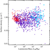 |
Fig. A.2 Surface density against L/M ratio for ALMAGAL targets. The colors and symbols are the same as in Figure 4. Notably, values of Σ < 0.1 g cm−2 are present in the ALMAGAL sample due to i) the inclusion of sources selected from the RMS catalog, which were not subject to the physical parameter constraints applied to sources from the Hi-GAL catalog (see Molinari et al. 2025, and Sect. 2 of this paper), and ii) the use of source sizes in this work that have not been beam-deconvolved when deriving surface densities, differing from the original ALMAGAL target selection criteria. |
Appendix B Testing a prediction for the number of cores versus distance behavior
In this appendix, we test the prediction made by Baldeschi et al. (2017) about the number of cores detected in a clump as a function of the distance. They found
![Mathematical equation: $\[N_{\text {core }}(d)=N_0\left(d_0 / d\right)^\delta,\]$](/articles/aa/full_html/2026/01/aa54764-25/aa54764-25-eq4.png) (B.1)
(B.1)
where N0 is the number of cores detected at a distance d0 < d, and with δ varying with the Herschel band.
The way Eq. (B.1) can be applied here is by considering a clump as a structure appearing as a single object (then N = 1) at its distance d, and imagining the increase in resolution from Hi-GAL (~18″ at 250 μm) to ALMAGAL (using 0″.3 corresponds to a factor of 60), as it was produced by approaching the source by the same factor (i.e., d/d0 = 60). Adopting a typical exponent δ = 1.5 for 250 μm quoted by Baldeschi et al. (2017), one should then expect ~460 cores inside one clump, which is extremely far from what is actually found in the observations (Ncore < 50).
To explain this discrepancy, one has to take into account that:
Both factors opposing fragmentation (turbulence, magnetic field, and feedback) and the decrease in sensitivity with distance (not accounted for in the realizations of Baldeschi et al. 2017) surely contribute to a decrease in the number of observed cores.
Eq. (B.1) was empirically determined by probing shorter ranges of ratios between original and “moved away” distances (d/d0 ≲ 30), and, probably, is not fully adequate for this test.
Connected to the previous point, a limit of this check is to consider that the confusion of the N cores in one clump is achieved at distance d, but actually, depending on the source disposition across the ALMAGAL FOV (35″), it can be observed also at closer distances, making the d/d0 much smaller than 60. That said, however, to extrapolate Ncore = 49 (the maximum value achieved in the ALMAGAL catalog), or – say – 10, much lower distance ratios should be invoked (~13 and ~5, respectively).
Appendix C Comparing surface densities of clumps and cores
The relationship between the clump average surface density (Σ) and the surface density of the cores within is worth examining. By definition, we expect each clump to contain at least one core whose surface density exceeds the clump’s average.
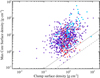 |
Fig. C.1 Surface density of the densest core in a clump versus clump average surface density. The symbols are the same as in Figure 17. The dotted and dashed lines represent the 1:1 and 1:3 relations, respectively. |
To test this, Figure C.1 plots the maximum surface density found in each clump (which in 88% of cases corresponds to the surface density of the MMC) against Σ. The plot reveals no strong correlation between these quantities. The key observation remains that the maximum core surface density generally exceeds the clump’s average surface density. In the remaining 2% of cases where this condition is not met, the ratio between core and clump surface densities falls within a range of 1/3 to 1 (a similar result can be found in Merello et al. 2015).
These discrepancies can be attributed to uncertainties in core mass estimates (and, consequently, surface densities) as discussed by Coletta et al. (2025). Additionally, the systematic difference in the dust opacity values used for calculating core and clump masses, as pointed out in Section 5, can account for a factor of ~2, thereby explaining most of the observed discrepancies.
Appendix D Skimming the ALMAGAL sample for potential free-free emission contamination
Coletta et al. (2025) discuss the impact of free-free emission contamination on millimeter continuum flux measurements of cores, as it can lead to an overestimation of the core mass. Coletta et al. (2025) exclude from their analysis of the core mass function all cores associated with CORNISH or CORNISH South cm free-free emission. Additionally, they also omit cores within ALMAGAL targets falling outside the coverage areas of these two surveys, where information on the possible presence of radio emission is unavailable.
In this appendix, we assess the potential impact of this contamination on our analysis. First of all, it is important to note that the degree of fragmentation is unaffected by this issue, so our focus here is solely on the mass of the MMC (MMMC) and the CFE. In particular, we examine how the plots in Figures 7 and 14 change after excluding ALMAGAL targets where free-free contamination has been confirmed for at least one core by Coletta et al. (2025), as well as targets outside the coverage of the CORNISH and CORNISH South surveys. For conciseness, we present only four of the six clump properties used to construct the aforementioned figures: M, Σ, L/M, and T.
In this context, Figure D.1 contains the plots of MMMC versus these four clump parameters, limited to the sources presenting no radio free-free contamination (or risk thereof). Two potential biases must be considered when comparing Figures D.1 and Figure 7. First, excluding sources possibly contaminated by free-free emission tends to rule out preferentially more evolved targets, which are characterized by higher values of L/M and T, resulting in a relative depopulation of the right side of panels c and d in Figure D.1. Second, if the continuum emission from the MMC of a given clump is affected by contamination, its flux density – and consequently MMMC – will be overestimated. However, removing contaminated objects does not necessarily imply the exclusion of the highest values of MMMC.
That said, the same considerations made in Sect. 4 regarding the trends of MMMC versus clump properties appearing in Figure 7 remain applicable to the plots in this figure, as they exhibit similar qualitative behavior. Noticeably, for this restricted sample, the slope of the power-law fit for MMMC versus Σ changes from 0.75 ± 0.06 (Sect. 4.2) to 0.64 ± 0.07, which remain consistent within the error bars. Furthermore, out of 31 clumps with MMMC > 24 M⊙ (Sect. 6.2.1), only 18 do not present free-free contamination.
A similar behavior can be seen also for CFE, by comparing Figures D.2 and 14, as the monotonic nature of observed median trends remains unchanged across all plots after ruling out possible cases of free-free contamination. In particular, in more quantitative terms, in Sect. 5.3 we fit a power law to the plot of CFE versus L/M and T, obtaining the exponents 0.36 ± 0.02 and 2.5 ± 0.1, respectively. Repeating this procedure for the plots in panels c and d of Figure D.2, we obtain a power-law dependency as 0.37 ± 0.02 and 2.6 ± 0.1, respectively, which are fully consistent with the previous ones, within the error bars.
In conclusion, whereas an analysis based on core masses should ideally exclude instances of possible mass overestimation due to free-free contamination, in practice the general indications taken from the subsample, selected by applying stricter constraints, are consistent with those found in the full sample. Therefore, we can confidently affirm the validity of conclusions drawn in the current paper for the entire ALMAGAL sample.
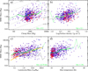 |
Fig. D.1 Plots of MMMC versus clump mass (a), surface density (b), L/M ratio (c), and temperature (d), after ruling out both ALMAGAL targets with at least one contained core found by Coletta et al. (2025) to be contaminated by radio emission from CORNISH or CORNISH South data, as well as ALMAGAL targets lying outside the areas of the sky covered by these two surveys. The symbols, colors, and lines are the same as in panels b, c, d, and e, respectively, of Figure 7. |
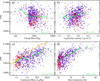 |
Fig. D.2 Same as Figure D.1, but for the CFE on the y-axis. The symbols, colors, and lines are the same as in panels b, c, d, and e, respectively, of Figure 14. |
Appendix E Calculating the Spearman’s critical value for 5% significance level and n = 840 data points
The critical values of Spearman’s rank correlation coefficients (ρS) are typically tabulated for sample sizes up to n = 100 (e.g., Zar 1999). As n further increases, these critical values tend to exhibit asymptotic behavior. For large n, the distribution of Spearman’s approximates that of Student’s t distribution, according to the following relationship(e.g., Ramsey 1989):
![Mathematical equation: $\[t=\rho_{\mathrm{S}} \sqrt{\frac{n-2}{1-\rho_{\mathrm{S}}^2}}.\]$](/articles/aa/full_html/2026/01/aa54764-25/aa54764-25-eq5.png) (E.1)
(E.1)
For n = 840, and a significance level of 5% (corresponding to 2.5% in each tail for a two-sided test, i.e., p = 0.025), the critical t value is tcrit = 1.963. Applying the inverse of the equation above,
![Mathematical equation: $\[\rho_{\mathrm{S}}=\frac{t}{\sqrt{t^2+n-2}},\]$](/articles/aa/full_html/2026/01/aa54764-25/aa54764-25-eq6.png) (E.2)
(E.2)
yields a critical ρS value of ρcrit ≃ 0.07, i.e., the value reported in Sect. 6.1.
Following the same procedure, but at a significance level of 99.7% (i.e., 3-σ), the critical t-value is tcrit = 3.89, yielding ρcrit ≃ 0.13.
All Tables
Summary of recent studies on clump fragmentation carried out on interferometric data of continuum emission.
Statistics of core population parameters (namely fragmentation level, mass of the MMC, and CFE).
Median photometric and physical parameters of the entire ALMAGAL sample and subsamples with and without cores.
All Figures
|
Fig. 1 Example of an ALMAGAL target observed from mid-infrared to millimeter. The ALMAGAL ID (AG323.7408-0.2633), its physical parameters (Molinari et al. 2025), and the number of cores detected in ALMAGAL continuum observations (Coletta et al. 2025) are reported in the top-left corner of the figure. Panels a–h: source images (~80″ × 45″) at wavelengths increasing from 24 μm to 1.38 mm. The wavelength in micrometers is reported in the top-right corner of each panel. Panel a: Spitzer-MIPS image of the source (saturated in the center). Panels b and c: Herschel-PACS images. Panels d–f: Herschel-SPIRE images. Panel g: the ATLASGAL image. Panel h: new ALMAGAL image. In this image, 15 fragments were detected by Coletta et al. (2025). Angular resolutions in the different panels are as follows: a: 6″; b: 10.2″ (for this panel and the following four, the resolution value is not the nominal one for Herschel, but rather the one directly measured by Traficante et al. 2011, on Hi-GAL maps, and circularized here); c: 13.5″; d: 23″; e: 30″; f: 42″; g: 19″; and h: 0.5″. Being detected at 70 μm (and also at 24 μm, in this case), this source is classified as star-forming in accordance with the Hi-GAL catalog criteria. |
| In the text | |
|
Fig. 2 Distributions of ALMAGAL target physical properties: (a) heliocentric distance; (c) mass (common logarithm); (e) surface density (common logarithm); (g) bolometric luminosity over mass ratio (common logarithm); (i) modified blackbody temperature; and (k) bolometric temperature. Panels b, d, f, h, j, and l: corresponding cumulative distributions. Three different populations are shown separately: in red, quiescent (70-μm dark) clumps; in blue, star-forming (70-μm bright) clumps; and in cyan, star-forming clumps associated with an UC HII region (notice that, differently from Elia et al. 2017, 2021, the counts of the third class of objects are not also included in those of the second class). All histograms are normalized by their total (116, 817, and 74 sources, respectively); therefore, they do not mirror the actual number ratios between clump classes. Units on the y-axis are arbitrary. Additionally, in the panels containing the cumulative distributions, the red and dotted curves correspond to the subsamples of quiescent and star-forming clumps with no detection of millimeter cores in ALMAGAL observations (discussed in Sect. 3.5). UCHII regions are not shown, as only one appears devoid of cores inside. |
| In the text | |
|
Fig. 3 Properties of ALMAGAL targets as a function of the number of cores (Ncore) revealed in their interior. Top: fluxes in the five Hi-GAL bands and their averages in bins of ΔNcore = 1. The core-band correspondence is reported in the legend. Middle: temperature determined using a modified-blackbody fit to the Hi-GAL SEDs and its average. Bottom: as in the top panel, but for the product of flux densities and the squared distance. In both the top and bottom panels, a break in the red curve corresponds to a bin populated by sources without a 500 μm detection. |
| In the text | |
|
Fig. 4 Number of fragments Ncore detected in each ALMAGAL target as a function of the target’s physical parameters: (a) heliocentric distance, with the vertical dotted line separating the distances originally assigned to the “near” and the “far” sample (see text); (b) mass; (c) surface density (logarithm); (d) luminosity over mass ratio, with the orange line representing the model prediction from Lebreuilly et al. (2025) with initial conditions set to M = 500 M⊙, ℳ = 7, and μ = 10 (presented and discussed in Sect. 6.2.2); (e) modified blackbody temperature; and (f) bolometric temperature, respectively. The open red triangles represent quiescent clumps; open dark blue diamonds represent star-forming clumps; and light blue-filled circles represent counterparts of a UCHII region. The symbol under each panel represents the typical error bar associated with the data. In this case, the vertical error bar is replaced by an arrow to indicate the number of detected cores likely representing an underestimate of the “actual” Ncore. The green line connects the medians of Ncore in bins (whose width is specified in green as well); its dotted parts correspond to bins containing low statistics (less than ten values). In panel c, medians calculated in bins of surface densities but based on deconvolved clump sizes are also represented as a dark solid or dotted green line. The mean values are also shown, connected by a magenta line. |
| In the text | |
|
Fig. 5 Top: statistical distribution of the fragment number Ncore for the ALMAGAL targets, categorized into quiescent (red histogram), star-forming (blue), and CORNISH-based UCHII regions (light blue). The sum of each histogram is normalized to 1; therefore, all histograms subtend the same area and do not reflect the actual numerical proportions among the classes. The three vertical dashed lines indicate the medians of these distributions, calculated excluding cases where Ncore=0. Bottom: cumulative distributions corresponding to the histograms shown in the top panel. The cumulative distribution of Ncore for star-forming targets located within the regions covered by the CORNISH and CORNISH South surveys is also shown (dotted blue) to highlight the potential impact of contamination from UCHII regions (see text). |
| In the text | |
|
Fig. 6 Top: histograms of Hi-GAL PACS flux densities (dark blue: 70 μm; light blue: 160 μm) for ALMAGAL targets with and without the detection of cores (dotted and solid line, respectively). The median values for the two subsamples are shown as vertical dashed and solid lines of the same color, respectively. Middle: same as in the top panel, but for SPIRE flux density distributions (green: 250 μm; yellow: 350 μm; and red: 500 μm). Bottom: cumulative distributions of histograms shown in the top and middle panels, using the same color and line style convention. |
| In the text | |
|
Fig. 7 Same as Figure 4, but for the MMC mass along the y-axis of each panel. The symbol under each panel represents the typical error bar associated with the data. The dotted gray lines in panel b indicate the trends for constant fMMC values. In panel c, the solid gray line indicates the power-law fit to the data, and the open yellow triangles represent data from Morii et al. (2023). In panel d, the gray line represents the median mass of the least massive core in each clump. |
| In the text | |
|
Fig. 8 Mass of the MMC vs. clump mass for ALMAGAL (open blue diamonds) and CORNISH (South) (light blue-filled circles) star-forming targets, limited to 8 × 10² M⊙ < M < 2 × 10⁴ M⊙ and 1 × 10⁴ L⊙ < L < 6 × 10⁵ L⊙. The green line connects the medians of MMC mass in logarithmic bins of 0.2 for the entire sample (as in Figure 7, panel b), while the gray line is recalculated only with the points plotted here. Furthermore, magenta-filled squares represent the values by Xu et al. (2024a). |
| In the text | |
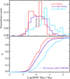 |
Fig. 9 Same as Figure 5, but for the mass of the MMC instead of the number of cores. |
| In the text | |
|
Fig. 10 Mass of the MMC versus the level of fragmentation for ALMAGAL targets. The symbol and color-coding used for source subclasses is the same as in Figure 4 and throughout the paper. The green line represents the median in bins of ΔNcore = 2. |
| In the text | |
|
Fig. 11 Clump bolometric luminosity L plotted against the fragmentation level (top left), mass of the MMC (top right), mass of the MMC normalized by the square of the distance (with luminosity normalized as well, bottom left), and sum of core masses (bottom right). The symbol and color-coding used for source subclasses is the same as in Figure 4 and throughout the paper. In the top-right and bottom-right panels, the green line represents the median in bins of the quantity on the x-axis. |
| In the text | |
|
Fig. 12 Top: CFE against clump angular size, estimated from Herschel photometry at 250 μm. The symbols are defined as in Figure 4. The green line connects the median of the size estimated in bins of 2″. The vertical dotted line represents the diameter of the ALMAGAL FOV. Bottom: same as in the top panel, but for the clump mass on the y-axis. |
| In the text | |
|
Fig. 13 Top: CFE against mass of the MMC (MMMC). Symbols are defined as in Figure 4. Bottom: distribution of the ratio between the mass of the MMC and the total mass contained in cores (excluding clumps with Ncore=0 or 1), shown separately for quiescent (red histogram), star forming (blue), and UCHII regions (cyan). The dashed curves represent the corresponding cumulative distributions, with values referenced to the y-axis on the right side of the plot. The vertical dotted lines mark the median values for each subclass, using the same color scheme as the histograms. |
| In the text | |
|
Fig. 14 Same as Figure 4, but for the CFE along the y-axis of each panel. In addition, in panels d and e, the gray solid lines represent the best power-law fit to data. |
| In the text | |
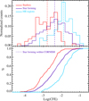 |
Fig. 15 Same as Figure 5, but for the CFE instead of the number of cores. |
| In the text | |
|
Fig. 16 Matrix of Spearman’s correlation coefficient ρS for relationships between clump physical parameters (x-axis) and core population parameters (y-axis). The color scale goes from dark orange (ρS = −1) to dark purple (ρS = 1) through white (ρS = 0). |
| In the text | |
|
Fig. 17 Same as panel d of Figure 7, but with different symbols and color-coding. The color scale is coded according to the logarithm of the clump surface density in grams per square centimeter (color bar on the right), and quiescent clumps (SL in the legend in the top-left corner), star-forming ones (SF), and UCHII counterparts (HII) are displayed by means of open triangles, open diamonds, and filled circles, respectively. The symbol size scales as the logarithm of the mass of the MMC, as shown in the legend. The solid gray line represents the numerical prediction by Lebreuilly et al. (2025) with initial conditions set to M = 500 M⊙, ℳ = 7, and μ = 10, also plotted in panel e of Figure 7 as an orange line. |
| In the text | |
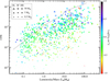 |
Fig. 18 Same as Figure 17, but for the CFE on the y-axis. |
| In the text | |
|
Fig. A.1 Volume density vs. surface density relation for ALMAGAL targets. The colors and symbols are the same as in Figure 4. |
| In the text | |
|
Fig. A.2 Surface density against L/M ratio for ALMAGAL targets. The colors and symbols are the same as in Figure 4. Notably, values of Σ < 0.1 g cm−2 are present in the ALMAGAL sample due to i) the inclusion of sources selected from the RMS catalog, which were not subject to the physical parameter constraints applied to sources from the Hi-GAL catalog (see Molinari et al. 2025, and Sect. 2 of this paper), and ii) the use of source sizes in this work that have not been beam-deconvolved when deriving surface densities, differing from the original ALMAGAL target selection criteria. |
| In the text | |
|
Fig. C.1 Surface density of the densest core in a clump versus clump average surface density. The symbols are the same as in Figure 17. The dotted and dashed lines represent the 1:1 and 1:3 relations, respectively. |
| In the text | |
|
Fig. D.1 Plots of MMMC versus clump mass (a), surface density (b), L/M ratio (c), and temperature (d), after ruling out both ALMAGAL targets with at least one contained core found by Coletta et al. (2025) to be contaminated by radio emission from CORNISH or CORNISH South data, as well as ALMAGAL targets lying outside the areas of the sky covered by these two surveys. The symbols, colors, and lines are the same as in panels b, c, d, and e, respectively, of Figure 7. |
| In the text | |
|
Fig. D.2 Same as Figure D.1, but for the CFE on the y-axis. The symbols, colors, and lines are the same as in panels b, c, d, and e, respectively, of Figure 14. |
| In the text | |
Current usage metrics show cumulative count of Article Views (full-text article views including HTML views, PDF and ePub downloads, according to the available data) and Abstracts Views on Vision4Press platform.
Data correspond to usage on the plateform after 2015. The current usage metrics is available 48-96 hours after online publication and is updated daily on week days.
Initial download of the metrics may take a while.