| Issue |
A&A
Volume 705, January 2026
|
|
|---|---|---|
| Article Number | A191 | |
| Number of page(s) | 30 | |
| Section | Stellar structure and evolution | |
| DOI | https://doi.org/10.1051/0004-6361/202554956 | |
| Published online | 20 January 2026 | |
Validating a non-local stellar convection model with 3D hydrodynamics simulations
1
Heidelberger Institut für Theoretische Studien Schloss-Wolfsbrunnenweg 35 69118 Heidelberg, Germany
2
Max-Planck-Institut für Astrophysik Karl-Schwarzschild-Straße 1 85748 Garching, Germany
3
Zentrum für Astronomie der Universität Heidelberg, Astronomisches Rechen-Institut Mönchhofstr. 12–14 69120 Heidelberg, Germany
4
Zentrum für Astronomie der Universität Heidelberg, Institut für Theoretische Astrophysik Philosophenweg 12 69120 Heidelberg, Germany
★ Corresponding author: This email address is being protected from spambots. You need JavaScript enabled to view it.
Received:
1
April
2025
Accepted:
3
October
2025
Abstract
Context. The efficient transport of energy and chemical elements by convective motions has a profound effect on the structure and evolution of stars. These motions occur on the relatively short dynamical timescale of convection and are intrinsically multi-dimensional. Stellar models usually rely on the one-dimensional mixing-length approximation of these processes, which is known to break down at convective boundaries. The Kuhfuß, R. (1987, Dissertation, Technische Universität München, München) convection model has been shown to handle convective boundaries in a more consistent way.
Aims. We test the assumptions that enter the Kuhfuß model using multi-dimensional hydrodynamics simulations, and we compare the results with existing one-dimensional models. Where possible, we also aim to calibrate the parameters of the Kuhfuß model using the simulations.
Methods. We computed one-dimensional stellar models employing the Kuhfuß model of a 3 M⊙ main-sequence star. These models were compared to three-dimensional hydrodynamic simulations obtained with the code called SEVEN-LEAGUE HYDRO and using the Reynolds-averaged Navier Stokes analysis. We analysed the global convective variables and individual contributions to the equations of the convection model.
Results. The turbulent kinetic energy as predicted by the Kuhfuß model agrees well with the simulation results. Towards the boundary of the convective core, the simulations show a layer of a positive entropy gradient that coincides with a positive convective flux, as predicted by the convection model. The terms involving pressure fluctuations are found to have a non-negligible magnitude.
Conclusions. The agreement of the turbulent kinetic energy equation for the convection model and the simulation is an important sign that the convection model is physically accurate. The gradient of the mean entropy that we found in the multi-dimensional simulations and in the Kuhfuß model confirms the existence of a Deardorff layer, that is, of a layer with a subadiabtic temperature stratification and positive convective flux. This is not predicted by the mixing-length theory. The assumption that turbulence is isotropic and that pressure fluctuations are negligible needs to be revisited in the convection model.
Key words: convection / hydrodynamics / stars: evolution / stars: interiors
© The Authors 2026
 Open Access article, published by EDP Sciences, under the terms of the Creative Commons Attribution License (https://creativecommons.org/licenses/by/4.0), which permits unrestricted use, distribution, and reproduction in any medium, provided the original work is properly cited.
This article is published in open access under the Subscribe to Open model.
Open access funding provided by Max Planck Society.
1. Introduction
Although the assumption of hydrostatic equilibrium is mostly justified, the interiors of stars are inherently dynamic. They are subject to dynamic flows of gas driven by various physical processes. One of the most important contributions stems from convection, which is the transport of matter and energy by bulk fluid motions. The high transport efficiency of convection makes it a crucial ingredient in stellar structure and evolution models because convective layers have a nearly homogeneous composition, and deep convective layers are also nearly adiabatically stratified. In main-sequence stars, in which the nuclear burning is dominated by the CNO cycle, the energy transport in the core becomes convective. The extent of these convectively mixed cores has a direct effect on the luminosity, the chemical yield, and the lifetime of these stars as well as the final fate of the stars as supernovae and potential mergers of the stellar remnants.
The convection in stellar cores is an inherently multi-dimensional turbulent process. The governing equations are too complex for an analytical treatment, and we therefore have to resort to numerical solutions (e.g. Lecoanet & Edelmann 2023). This makes three-dimensional (3D) hydrodynamic simulations a powerful tool for studying stellar convection. These simulations solve the equations of gas dynamics numerically. As a result, the simulations provide us with a time series of hydrodynamic variables such as the velocity field, the mass density, or the specific energy density of the fluid in three spatial dimensions. Compared to other theoretical descriptions of hydrodynamics, 3D simulations apply a limited set of assumptions and approximations. For example, Lecoanet & Edelmann (2023) point out that kinetic energy spectra and average velocities agree well in different simulations. Therefore, 3D simulation results are considered as a rather accurate representation of the physical reality.
Numerical simulations of core convection still include a number of challenges (we refer to Lecoanet & Edelmann 2023 for a review of current simulations of core convection and its limitations; further limitations of core-convection simulations in the context of asteroseismic observations of F- and B-type stars were discussed by Aerts et al. 2021). Some of the main challenges are the long thermal timescale in contrast to the short convective timescale, the effects of rotation and magnetism, and the mixing of chemical elements by waves. Even though we model core convection here, we would like to point out that major challenges have been encountered in modelling convection in the Sun. This circumstance is known as the convective conundrum (e.g. Hanasoge et al. 2012; O’Mara et al. 2016). Currently, rotation and magnetism seem to play major roles in reconciling solar observations and simulations (Käpylä 2024, and references therin), while the helioseismic observations are also actively debated (Birch et al. 2024).
The construction of grids of 3D models that cover the whole range of parameters in stellar convection (stellar mass, age, composition, stratification, etc.) is prohibited by the enormous computing time needed. This necessitates an efficient model that accurately captures the physics of convection without relying on expensive 3D calculations. The first step towards building such a model and testing its accuracy is to compare the convection model to self-consistent 3D simulations. To analyse the 3D simulations and compare them to one-dimensional (1D) stellar models, we used the Reynolds-averaged Navier Stokes (RANS) analysis (e.g. Viallet et al. 2013; Arnett et al. 2015). The RANS equations are based on the so-called Reynolds splitting (Reynolds 1894),
 (1)
(1)
which splits the hydrodynamic variables such as the density ρ or velocities u into a mean part and a fluctuating part, which are denoted with the overbar and with the prime, respectively. Inserting the Reynolds splitting into the hydrodynamic equations allows us to construct the dynamic equations of the fluctuating quantities and higher-order combinations thereof. While the evolution equations of correlation functions of a given order are analytically exact, they cannot be solved self-consistently because correlations of an even higher order always arise from the non-linearity of the Navier-Stokes equation. So-called closure relations are therefore necessary to approximate these and other terms that are not described within the model to obtain a closed system of equations.
In contrast to 3D simulations, stellar structure and evolution models employ various assumptions and approximations, the most prominent being spherical symmetry. Hence, the hydrodynamic flows also need to be described in one spatial dimension. To compute accurate stellar models, it is crucial to ensure that the 1D models capture the most relevant aspects of the hydrodynamic flows. For decades, the most commonly used scheme to describe convection in stellar models has been the mixing-length theory (MLT) (Prandtl 1925; Biermann 1932; Böhm-Vitense 1958). Despite its simplicity as a local and time-independent theory, MLT has described stellar structure and evolution with great success. Evidence has accumulated in recent years, however, that MLT systematically underestimates the size of convective regions from an observational (Maeder & Mermilliod 1981; Bressan et al. 1981; Pietrinferni et al. 2004; Magic et al. 2010; Claret & Torres 2019; Mombarg et al. 2019; Pedersen et al. 2021; Deheuvels et al. 2016; Angelou et al. 2020) and a theoretical side (Roxburgh 1978, 1992; Zahn 1991; Meakin & Arnett 2007; Käpylä 2019; Higl et al. 2021; Anders et al. 2022; Andrassy et al. 2024). This has profound implications for the stellar structure and evolution modelling because the size of convective regions affects for example the properties of convective cores (Moravveji et al. 2015; Pedersen et al. 2021), the lithium abundance of the Sun and Sun-like stars (Carlos et al. 2019; Pinsonneault 1997; Dumont et al. 2021), the location of the base of the solar convection zone (Basu & Antia 2004; Christensen-Dalsgaard et al. 2011; Asplund et al. 2021; Braun et al. 2024), the location of the red giant branch bump (Alongi et al. 1991; Khan et al. 2018), and supernova explosions (Schneider et al. 2023; Heger et al. 2023; Temaj et al. 2024).
These shortcomings led to the introduction of convective overshooting to allow for chemical mixing, and in some descriptions, to also allow for a modified thermal stratification beyond the formal MLT boundaries in stellar models. So far, different approaches have been taken to introduce this convective overshooting in the stellar models, for example by simply extending the convectively mixed region by a fraction of the pressure scale height, by introducing an exponentially decreasing diffusion coefficient at convective boundaries (e.g. Freytag et al. 1996), or by increasing the size of mixed regions through convective entrainment (Turner 1986; Meakin & Arnett 2007). While these approaches are parametrised solutions to the problem, so-called turbulent convection models (TCMs) serve as an alternative description of convection to overcome the fundamental shortcomings of the MLT (Stellingwerf 1982; Kuhfuß 1987; Canuto 1992; Xiong et al. 1997; Canuto & Dubovikov 1998; Li & Yang 2001). Starting from the RANS equations and supplying the necessary closure relations, these models allow for time-dependent convective variables and introduce non-local terms that lead to convective regions extending beyond the formal MLT boundaries defined by a stability criterion.
We compare results from 1D stellar models including the Kuhfuß convection theory (Kuhfuß 1987) to the 3D simulations by constructing the convective variables and the individual equation terms from the 3D data using the RANS analysis. The original Kuhfuß (1987) model has recently been extended by Kupka et al. (2022) and Ahlborn et al. (2022) (K22 and A22 in the following) to include the dissipation by buoyancy waves at convective core boundaries. In this work, we use the version described by K22 and A22. We compare the Kuhfuß model in different ways to the hydrodynamic simulations. The first and simplest comparison is to directly compare the convective variables obtained from the stellar model and as extracted from the hydrodynamic simulations. Here, the turbulent kinetic energy (TKE) and the convective flux are most relevant for stellar structure and evolution because they determine the extent and thermal stratification of convective regions. With this approach, we test how well the stellar models represent the results obtained from the hydrodynamic simulations.
This comparison only shows global discrepancies, however, and does not indicate their physical origin. To study the causes for potential discrepancies of the convective variables in the 1D and 3D data, we compare the individual terms of the RANS equations computed in the simulations and stellar models (see Sects. 2 and 5). These terms can be directly compared to their 1D counterparts, obtained from the TCM, which again allows us to assess the overall physical accuracy of the TCM. Finally, the RANS analysis of 3D simulation data can be used to interpret the results of the simulation, as discussed by Viallet et al. (2013), Arnett et al. (2015), Mocák et al. (2018) or Horst et al. (2021). The comparison of the results of hydrodynamic simulations with the TCM in a stellar model is therefore a powerful way to identify shortcomings of the convection model and understand turbulent convection in stars in general (Grossman 1996; Cai 2020; Arnett et al. 2015; Kupka & Muthsam 2007a,b,c; Snellman et al. 2015).
With this comparison, we determine whether the Kuhfuß model in our current version is an acceptable model to describe convection in stars and if it describes the overshooting zone correctly. In A22 we discuss the agreement between the Kuhfuß model and other 1D descriptions of convective overshooting and observations. An early analysis of the 3D simulations presented in this work can be found in Ahlborn (2022). In Sect. 2 we describe the relevant RANS equations and the TCM by Kuhfuß (1987) and K22 in more detail. In Sect. 3 we describe the simulation code we used and the numerical setup of the simulations. In Sect. 4 we compare the convective variables to their representations computed from the 3D simulations. Subsequently, we compute the terms of the relevant RANS equations and compare them to their counterparts computed in the Kuhfuß model (Sect. 5). Based on the individual terms of the Kuhfuß model computed from the hydrodynamic simulations, we discuss how varying the model parameters might improve the agreement between the model and the simulations in Sect. 6. Because of the theoretical and numerical uncertainties of the hydrodynamic simulations, this analysis can be only carried out in the theoretical limits of the simulations we used (we refer to Sects. 3 and 7).
2. The Kuhfuß (1987) TCM
We used the TCM derived by Kuhfuß (1987) in the implementation described in K22 and A22 (we also refer to Flaskamp 2003). For the sake of completeness, we repeat the most important aspects of the model in this section. As most TCMs, the model of Kuhfuß (1987) is based on the Reynolds splitting (see Eq. (1)), where the fluctuating part refers to the turbulent contribution of the flow. For stellar structure and evolution models, higher-order combinations of these fluctuating parts are of particular interest. The Kuhfuß model features three convective variables that are second-order correlations of fluctuating quantities,
 (2)
(2)
 (3)
(3)
 (4)
(4)
where s′ refers to the fluctuations of the specific entropy. Here and throughout the rest of the paper, the overbar denotes a volume-weighted Reynolds average in contrast to a mass weighted Favre average. In the following, we refer to ω as the TKE, to Π = Πr (the radial component of the convective flux vector) as the convective flux variable and to Φ as the entropy fluctuation variable. By computing the higher-order correlation functions ω, Π and Φ, the Kuhfuß (1987) equations describe bulk properties of the flow in a statistical way. In the following we first describe how to derive the RANS equations by applying the Reynolds splitting to the Navier Stokes (Eq. A.1) and the energy conservation Equation (A.3). Subsequently, we describe the final equations of the Kuhfuß (1987) TCM. The resulting equations are also used to analyse the 3D simulation results.
2.1. The RANS equations
Given the dynamic equations of the fluctuating quantities u′ and s′ (Eqs. (A.2) and (A.4)), the dynamic equations for the second-order moments Eqs. (2)–(4) are derived using the product rule:  and similarly for the other second-order correlation functions where
  . In the following, we give all the terms of the RANS equations and identify their physical meaning next to the term (e.g. Kuhfuß 1987),
 (5)
(5)
where σ is the viscosity tensor and p denotes the pressure. The notion buoyancy term is motivated by the expansion of  in terms of density fluctuations. In the Kuhfuß model the density fluctuations are further expanded in terms of entropy fluctuations to arrive at the convective flux variable Π (see also Kuhfuß 1987; Ahlborn 2022). Here, we have also rewritten
  using the assumption of hydrostatic equilibrium, where g denotes the gravitational acceleration vector.
Similar to the equation for the TKE, the evolution equation for the convective flux variable can be derived as
 (6)
(6)
where  refers to the ith unit vector. Here, we denote the radiative flux with q, the temperature with T and the specific energy generation rate with ε.
Finally, the evolution equation for the entropy fluctuations is given as
 (7)
(7)
The RANS formalism as such is analytically exact. Provided all the data were available, all the terms in the RANS formalism can be evaluated. However, when turning the question around and attempting to use the RANS equations to predict the behaviour of correlation functions relevant for stellar evolution, some terms cannot be computed self-consistently within the theory. As can be seen, the resulting equations for the second-order moments ω, Π and Φ contain a term that is already of third order: The first term on the right-hand side, referred to as the non-local flux, is a third-order moment in the fluctuating quantities. These terms of the next higher order appear as a result of the non-linearity of the Navier Stokes equation. As a consequence, a series of averaged moment equations up to infinite order would be needed to describe the complete problem. This is, of course, computationally infeasible. To compute these terms, approximations and models have to be applied, known as closure relations. Finding suitable closure relations is the task of turbulence theory, which we describe in the next subsection.
2.2. The 3-equation model
In the Kuhfuß model, it is assumed that there are no mean flows, that is  . Furthermore, the spatial distribution of the TKE is assumed to be isotropic. The buoyancy terms are modelled in the Boussinesq approximation and pressure fluctuations are neglected (i.e. p′ = 0). Additionally, molecular viscosity is neglected (σ = 0) in all terms except the viscous dissipation term in Eq. (5). As we discuss below, viscous dissipation is modelled implicitly as a Kolmogorov cascade. This last point also implies that our 3D simulation code solves the same set of equations that the Kuhfuß model tries to describe. For the details, we refer to the original work of Kuhfuß (1987) (a short summary may be found in Appendix A of K22). The final model equations of the 3-equation model read
 (8)
(8)
 (9)
(9)
 (10)
(10)
where ∇, ∇ad, and Hp refer to the dimensionless model and adiabatic temperature gradient and the pressure scale-height, respectively. With cp we refer to the specific heat capacity at constant pressure. The symbol Λ refers to the dissipation length, that is discussed further below, and CD is a model parameter (default value  ). The default parameter values are obtained by calibrating the local and time-independent Kuhfuß model to the MLT. The flux terms of the RANS equations are denoted as ℱa with a = ω, Π, Φ. In the Kuhfuß model, they are described with a down-gradient approximation (Daly & Harlow 1970; Launder & Reece 1975; Xiong 1978; Li & Yang 2007),
 (11)
(11)
where αa are model parameters. We note, however, that there is no a priori argument for a specific value. Kuhfuß (1987) suggested a value of 0.25 for αω based on a ballistic overshooting picture and calibrated αΠ and αΦ to MLT in a local and stationary limit. In agreement with previous work (A22), we select the same value of αω, αΠ, αΦ = 0.3. The heat flux terms of Eqs. (6) and (7) are modelled using a dissipation timescale,
 (12)
(12)
where γR is a model parameter (default value  ), σB refers to the Stefan-Boltzmann constant and κ denotes the Rosseland opacities. A detailed discussion of the model parameters in the 3-equation model may be found in Sect. 6.
Using the convective flux from the convection model, we define the temperature gradient of the stellar model self-consistently from the energy conservation in the stellar model (e.g. Kippenhahn et al. 2012),
 (13)
(13)
The dissipation length-scale Λ is defined according to
 (14)
(14)
where
and
assuming an ideal gas to compute  . Here, c4 = c3/(c2cϵ) and c2 = 1.92, c3 = 0.3 are parameters (see Eq. (21) in K22 and Canuto & Dubovikov 1998) and α is the equivalent to the mixing length parameter in MLT. The parameter cϵ denotes the dissipation parameter of the convection model, that is cϵ = CD. For the details of the implementation of this dissipation length-scale, we refer to Sect. 2.3 of A22 (see also Wuchterl 1995).
The convective chemical mixing was modelled as a diffusive process. The diffusion coefficient is defined as
 (15)
(15)
following Langer et al. (1985), with a parameter αs that is discussed further below.
2.3. The 1-equation model
The 3-equation model may be simplified to a 1-equation model by introducing an approximation for the convective flux variable. Following the description of the MLT (e.g. Biermann 1932; Böhm-Vitense 1958), the convective flux variable is expressed proportional to the entropy gradient and a convective velocity scale. The entropy gradient can be expressed using thermodynamic relations assuming a homogenous composition,
 (16)
(16)
which allows us to express the convective flux variable as
 (17)
(17)
(see e.g. Kuhfuß 1986, 1987, or A22, Sect. 2.1). Here,  is a parameter whose value is calibrated by comparing the 1-equation local model to the MLT. When approximating the convective flux in Eq. (8) in this way it is only necessary to solve for the convective variable ω. We refer to this model as the 1-equation model. When applying the 1-equation model, the dissipation length is computed according to the approximation by Wuchterl (1995), that is c3 = 0 for the computation of Eq. (14).
3. Three-dimensional hydrodynamic simulations of stellar core convection
In this section, we give an overview of the numerical code we used to compute the 3D simulations and the specific setup of our simulations. Furthermore, we describe how the spherical averages are computed from the 3D data.
3.1. Initial stellar models
To set up the hydrodynamic simulation, we used results from 1D stellar structure models. For this purpose, we used the 1D Garching Stellar Evolution Code (GARSTEC, Schlattl & Weiss 1999; Weiss & Schlattl 2008). For the following analysis, we initialised two 3D simulations with different 1D stellar models of a 3 M⊙ main-sequence star at solar metallicity to understand the impact of the initial model on the simulation result. The first simulation was initialised with a model computed employing the Kuhfuß 3-equation theory as described in Sect. 2.2. For this model, we followed the procedure of A22. The second simulation was initialised with a starting model computed using MLT and ad hoc overshooting according to Freytag et al. (1996). For the overshooting we chose a parameter value of fOV = 0.02. For simplicity, we refer to the two 3D hydrodynamic simulations as the sim_k simulation and the sim_m simulation, respectively, for the remainder of this paper1. In Fig. 1 we show the temperature stratification of the convective core of our 1D models as dot-dashed lines. In the 3-equation model, the temperature gradient changes over a finite radial distance from the close to adiabatic regime in the convective core to the radiative regime in the envelope. The local nature of MLT causes a much more abrupt transition in the MLT model. Therefore, it is important to initiate hydrodynamic simulations with both models, in order to understand the influence of the initial temperature stratification on the outcome of the simulations. For long enough simulation times (on the order of the thermal timescale) the simulations are expected to reach a similar solution of the convective core structure. We discuss the implications of the different initial thermal stratification for the simulation results in Sect. 7. We picked stellar models with a central hydrogen abundance of Xc = 0.6975, which means that the star has reduced its initial hydrogen abundance by less than 1% in the centre. The hydrogen profiles of the two initial models are shown in the lower left panel of Fig. B.1. The temperature, pressure, and density of the two initial models can be found in the other panels of Fig. B.1.
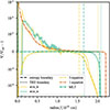 |
Fig. 1. Time-averaged superadiabaticity of the simulations (solid lines) and the initial models (dot-dashed lines). The dot-dashed orange line shows the superadiabaticity of the 1-equation model for comparison. The vertical dashed and dotted lines indicate the position of the entropy and TKE boundary (for definitions, see Sect. 4.1), respectively. |
These 1D models serve not only as initial models for the 3D simulations, but they are also used to directly compare TCM predictions with the simulation results. Following A22, we also constructed a corresponding 1D model with the 1-equation Kuhfuß model, which allows us to compare the simulation results with this TCM. In contrast to the MLT, the 1-equation model self-consistently develops an overshooting region around convective zones, as in the 3-equation model. The temperature gradient in these overshooting regions is close to being adiabatic (see A22 and Fig. 1). The extent of the overshooting region can be controlled by αω. We find that for αω = 0.15 the extent of the overshooting region of the 1-equation model matches the 3-equation model. So in total we compare the 3D simulations with three 1D stellar models, which we refer to as the MLT model, the 1-equation model, and the 3-equation model. As discussed above the MLT model includes ad hoc overshooting.
The 1D models used here do not include the effects of rotation or magnetic fields. Similarly, the sim_k and sim_m simulation do not include these effects. The 1D models do hence make the same assumptions about the underlying physics as the simulations. The Kuhfuß 1- and 3-equation models are a first step beyond MLT to take the effects of the turbulent flows into account. This allows us to study the effects of turbulent convection in isolation.
3.2. Simulation setup and numerics
For our 3D simulations of stellar core convection, we used the fully compressible SEVEN-LEAGUE HYDRO code (SLH, Miczek 2013; Edelmann 2014; Miczek et al. 2015), which solves the inviscid Euler equations of fluid dynamics with a finite volume scheme (see Edelmann et al. 2021, and references therein for the equations that get solved and details on the implementation). The SLH code follows the implicit large eddy simulations (ILES) approach, in which the smallest scales are filtered out, and only the larger, energy containing scales are simulated (e.g. Pope 2000). In ILES the physical dissipation lengthscale is not resolved by the simulation, but rather the numerical methods naturally dissipate the kinetic energy of the turbulent flows at scales close to the grid resolution element. Following Kolmogorov (1942), the flow properties at the integral and inertial scales remain unaffected by the details of the dissipation mechanism. The flows in stellar cores are highly subsonic, which makes compressible explicit time integration schemes computationally prohibitively expensive. We therefore used the implicit time integration scheme ESDIRK23 of Hosea & Shampine (1996). The low Mach number flows in the convective regions also required us to use a specialised flux function in order to avoid excessive dissipation (see for example the discussion in Miczek et al. 2015; Edelmann et al. 2021; Horst et al. 2021). For these simulations we applied the AUSM+-up flux function (advective upstream splitting method, Liou & Steffen 1993; Liou 1996, 2006). Overall the scheme is second-order accurate in time and space. We closed the system of equations with the Helmholtz equation of state including the ideal gas law and radiation pressure (Timmes & Swesty 2000), which differs from the OPAL EOS (Iglesias & Rogers 1996) used in the 1D models. Another important requirement for accurate simulations of hydrodynamic flows in the stellar interior concerns the state of hydrostatic equilibrium. Deviations from the hydrostatic equilibrium caused by an imperfect balance of pressure and gravity terms in the numerical scheme or the initial model may cause spurious flow velocities, which can dominate the physical flow. To avoid this, well-balancing schemes have been developed to numerically preserve the state of hydrostatic equilibrium over longer time. The deviation well-balancing scheme (Berberich et al. 2021) allows maintaining hydrostatic equilibria on the machine precision level by subtracting a reference state from the hydrodynamical quantities. The advantages of this scheme are demonstrated in Edelmann et al. (2021). The radiative flux was taken into account by means of a diffusion approximation. The opacity profiles were taken from the 1D stellar models and are not updated as the simulation evolves. The mean composition of the 1D models was taken over into the 3D simulations. We note, however, that the mixed regions of the 1D models extend further out in radius than the turbulent convective region in the 3D simulations, such that the convective region has uniform composition (see Table 1).
Comparison of different radial locations in the stellar models and simulations.
The SLH code has been used for several applications in stellar astrophysics, for example convective He-shell burning (Horst et al. 2021), the study of internal gravity waves (IGW) (Horst et al. 2020), shear instability (Edelmann et al. 2017), silicon burning (Röpke et al. 2018), convective core boundary mixing (Andrassy et al. 2024), and turbulent dynamo action (Leidi et al. 2023). Recently, Andrassy et al. (2022) carried out a code comparison study including SLH among other codes and demonstrated that all codes are in good agreement with each other for a convection setup of astrophysical relevance. Furthermore, SLH has been successfully applied to various test cases, for example a Gresho Vortex, the Kelvin Helmholtz instability, or a rising hot bubble (Miczek et al. 2015; Edelmann et al. 2021). This is an indication of the robustness of the numerical methods used. We hence conclude that the SLH simulations discussed in this work are fully suited for a comparison with 1D stellar models.
We set up the simulation in a wedge geometry in spherical coordinates with an extent of 45° in the θ direction and 45° in the ϕ direction. Each angular direction was discretised in 96 regularly spaced cells. In the radial direction, the wedge comprises approximately 2.5 × 1010 cm discretised using 384 regularly spaced grid cells. It has been shown previously that ILES results converge to the Kolmogorov scaling described above with increasing resolution (Cristini et al. 2017; Horst et al. 2021; Lecoanet & Edelmann 2023). Horst et al. (2021) used SLH to simulate He-shell burning in a massive star on a very similar grid configuration as in our case. The latter authors show that the RANS analysis already converges at their lowest resolution. Similar conclusions were reached by Cristini et al. (2017) for their RANS analysis. Further results by Andrassy et al. (2022, 2024) demonstrate that SLH results converge to the scaling for an increased resolution, as describe above. In our case, the convection zone is covered by about 300 points in the radial direction, and hence better resolved than in these simulations at their respective lowest resolution.
The multi-dimensional grid spans 1.16 pressure scale heights in the radial direction and 0.38 pressure scale-heights above the formal Schwarzschild boundary of the stellar models. In the very centre, a region of 109 cm (i.e. approximately 4% of the radial extent of the grid) was cut out to avoid the coordinate singularity of spherical coordinates. In the θ and ϕ direction, periodic boundaries were applied. In the radial direction, wall boundaries were used, that is, the velocity component perpendicular to the boundary is set to zero such that the flow turns sideways. The 1D initial stellar models described in Sect. 3.1 were mapped as a background into the 3D simulation following the procedure described by Edelmann et al. (2017). The model was first interpolated from the Lagrangian grid onto the Eulerian grid, which causes deviations from the initially perfect hydrostatic equilibrium. Subsequently, the density of the interpolated model was changed to reinstate a perfect hydrostatic equilibrium. In this process, the temperature stratification was forced to match the temperature stratification of the initial 1D stellar model. This last step is mainly necessary due to small differences of the EOS between GARSTEC and SLH. We did not follow the nuclear evolution of the H-burning core, since the estimated change in hydrogen abundance during the simulation time is completely negligible. Instead, we included the energy generated by nuclear fusion by a time constant heating profile. The radial distribution of the heating rate was taken from the initial stellar model. Both 3D simulations were evolved over approximately 104 h of physical time. The convective flow was seeded by introducing sinusoidal pressure perturbations with a relative amplitude of 10−7. Figure 2 shows the time evolution of the angularly averaged velocity magnitude throughout the domain. This illustrates how this perturbation slowly builds up into a turbulent flow before it reaches a quasi-steady state after approximately 2 × 10³ h. We exclude this initial transient phase from our analysis, such that our averaging interval consists of approximately 8 × 10³ h elapsed time in the simulation. This is only a small fraction of the Kelvin Helmholtz timescale at the Schwarzschild boundary of approximately 2.5 × 10⁵ years. The implications of this mismatch of timescales for the interpretation of the simulation results and the comparison to the 1D models are discussed in Sect. 7. Given current numerical methods it is, however, not possible to simulate a substantial fraction of this timescale at the nominal stellar luminosity.
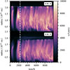 |
Fig. 2. Time evolution of the angularly averaged velocity profile. The top and bottom panels show the sim_m simulation and the sim_k simulation, respectively. The end of the initial transient phase is indicated with a vertical dashed white line. |
In Fig. 3 we show a representation of the convective flow in slices through the computational domain. We indicate the formal Schwarzschild boundary, which we define as the radial location where ∇ad = ∇rad, of the initial models with a white dash-dotted line in each panel. The results of the sim_k and sim_m simulation are shown in the left and right column, respectively. The upper panels show a slice in the x–z plane rotated by π/8 around the vertical axis, and the lower panels show a slice in the x–y plane. The Mach number is colour coded on a logarithmic scale. As discussed above, the Mach number of flows in convective cores on the main sequence is low and indeed does not exceed approximately 3 × 10⁻⁴ in the present simulations. The convective flows shown in Fig. 3 present a clear separation of spatial scales. This result arises from the use of specialised flux functions in SLH, which dramatically reduce the excessive amount of numerical dissipation typical of standard methods for fluid dynamics when used to model highly subsonic flows (Miczek et al. 2015; Edelmann et al. 2021). Without using a low-Mach solver, the problem of core convection in upper main sequence stars could only be studied with the so-called enhanced luminosity method (ELM; e.g. Käpylä et al. 2023, and references therein). The idea behind ELM is to artificially boost the driving luminosity of the convection by a large factor to considerably increase convective velocities and in turn the Mach number. In fact, in mildly subsonic regimes (Ma ∼ 0.01 − 0.1), standard shock-capturing methods can still provide accurate numerical results (Andrassy et al. 2022). However, altering the driving luminosity would also change the thermal structure of the relaxed model, which implies that we would no longer be testing properties of the Kuhfuß model2.
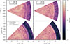 |
Fig. 3. Visualisation of the convective flow from the 3D simulations in the x–z and the x–y plane using the Mach number of the flow in the upper and lower panel, respectively. The results from the sim_k simulation are shown in the left column and the results from the sim_m simulation are shown in the right column. The Mach number is indicated with the logarithmic colour-scale. The Schwarzschild boundary of the initial stellar models is indicated with a white dash-dotted line in each panel. We further indicate the entropy and TKE boundary of each simulation with the dashed and dotted white lines (see Sect. 4.1 and Table 1 for details). The upper row shows the raw simulation data, while a radial smoothing has been applied to the flow velocities in the bottom row (see text). The Cartesian coordinates x, y, z are obtained from the conventional conversion of the spherical coordinates r, θ, ϕ of the simulation grid. |
We note that in the sim_k simulation, the turbulent convective motions seem to cease at a radius of about 1.9 × 1010 cm. Beyond this point, we observe that the motions are more ordered, related to internal gravity waves (e.g. Aerts et al. 2010). Beyond 2.05 × 1010 cm motions substantially decrease related to the formal Schwarzschild boundary of the initial models. In the sim_m simulation the turbulent convective motions extend until the Schwarzschild boundary, whereafter an abrupt drop of motions is visible. At the edge of the turbulent convective region, beyond the formal Schwarzschild boundary, some spurious velocity features are visible in the top row of Fig. 3. Our spatial resolution in the radial direction is 6.3 × 107 cm, yet the radial wavelength of IGW with a frequency corresponding to the convective turnover frequency and an angular degree of l = 8 is 2.6 × 107 cm in the stable layer. Moreover, the expected radial wavelength of IGW scales approximately as 1/l (Ratnasingam et al. 2020). All IGW in the stable layer are therefore critically under-resolved. In our numerical scheme, this leads to an odd-even pattern in the radial velocity with unrealistically large amplitudes. Close to the convective boundary waves with l = 8 are still resolved with five radial grid points per wavelength at the convective turnover frequency. However, higher angular orders and lower frequencies are also under-resolved at the convective boundary. Increasing the spatial resolution to resolve these waves is computationally unfeasible and beyond the scope of this project. However, the numerical effect of under-resolved waves can be easily filtered out of the simulation data by applying a smoothing kernel in the radial direction for cell xi,
 (18)
(18)
We applied this smoothing for the velocity and pressure components of the simulation data. The smoothing reduces the amplitudes of the numerical artefacts by a factor of approximately 100 and reveals the underlying wave motions, as can be seen in the bottom row of Fig. 3. The effect on the convective region is negligible. The extent of the turbulent convective region is discussed in more detail below. No data are available below x = 0.1 × 1010 cm, as this is outside of the lower edge of the computational domain.
3.3. Computation of averages
The hydrodynamic simulations provide us with time series of hydrodynamic variables in three spatial dimensions. To compute the RANS equations described in Sect. 2 and compare the 3D data with the stellar convection models, we need to compute suitable averages. In addition to the spatial average, we also computed a temporal average following Mocák et al. (2018). The resulting average then reads
where dΩ = sin θ dθ dϕ denotes the solid angle in spherical coordinates, τ and ΔΩ refer to the time interval and the solid angle that are averaged over, respectively. The initial time-interval needed for convection to fully establish is denoted as τ0. This interval is excluded from the averaging to avoid spurious results from this transient phase. The final average  is then time-independent, as we integrate over the remaining simulation time. We note that both convection models we want to compare to are time-independent. The MLT is time-independent by construction, and for the Kuhfuß equations we chose to neglect the time-derivatives. Therefore, the time-dependence in the simulations is not of interest for us at the moment. In Appendix C, we give some useful identities for the computation of the averages.
In order to get reliable results, τ has to be chosen large enough to average over statistical fluctuations in the turbulent flow. A natural timescale for this is the convective turnover time τconv defined as
 (19)
(19)
where L is the radial extent of the convective region and  is the space-time average of the velocity magnitude in that region. In our simulations, τconv has a typical value of 1500 h. Space-time averages of quantities directly related to the stratification of the 1D model used to initialise the simulation like density, pressure, or entropy are converged over much smaller timescales than τconv since they evolve on longer timescales and are hence not strongly influenced by turbulent motions. Perturbations of these quantities and dynamical quantities like velocities, on the other hand, evolve on the dynamical timescale and the appropriate size of the time averaging window needs to be estimated.
In Fig. 4 we compare averages of several quantities that evolve on a dynamical timescale. We show averages starting from τ0 = 2267 h with increasing τ ranging from one to five τconv. We find that correlations of perturbations of slowly evolving quantities like  converge quickly to a stable solution. The same cannot be said about the azimuthal component of the velocity vector (uϕ). Even after averaging over five convective turnover times, the values keep changing significantly. The reason for this is that the initial model corresponds to a non-rotating star and hence the averaged angular velocities should be close to 0. However, in non-rotating simulations the formation of a large-scale dipolar feature in the turbulent flow has been observed (see e.g. Gilet et al. 2013; Cristini et al. 2017; Meakin & Arnett 2007; Woodward et al. 2019). As we ran our simulations on a wedge geometry instead of a full-sphere, we cannot resolve this large scale dipolar feature. The non-zero velocity component in
  that we observe in our simulations originates from the periodic boundary conditions employed. Because the adopted numerical scheme introduces little dissipation, the resulting horizontal flow can remain coherent, mimicking a rotational component. This feature evolves slowly over many τconv. We would expect that
  should get close to 0 if we could extend our simulations to a significantly longer timescale. A non-zero mean velocity component is also in conflict with one of the main assumptions of the Kuhfuß model, which assumes
  .
.
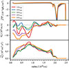 |
Fig. 4. Comparison of |


Despite the non-converging velocity average we find that the azimuthal component of the kinetic energy  still converges once we average over three to five τconv. This indicates that the magnitude of the velocity field is well converged as well. The same is true for the convective variables, and the superadiabaticity in the bulk of the convection zone. This is further discussed in Appendix D. We hence conclude that variables related to the convective velocity field reached a statistically stationary state on the dynamical timescale, given the thermal stratification.
For the following analysis, we averaged all profiles over five τconv. Even though the simulations are converged on the dynamical timescale, we still observe a secular evolution of quantities (e.g. the thermal stratification towards the boundary of the convective core in the lower panels of Fig. D.1 or the radial extent of the turbulent convective region) over the simulation time span. We attribute this to the different thermal stratifications in our two initial stellar models. To arrive at a consistent thermal and velocity structure independent of the initial models, simulation times on the order of the thermal timescale would be needed (e.g. Andrassy et al. 2024). This is illustrated in Fig. 1, which shows that the two simulations still have a different mean thermal stratification in the convective boundary layer. Together with the dynamical convergence, this makes results in the bulk of the convection zone and related to the dynamical evolution more robust than those obtained in the boundary layer and dependent on the thermal stratification. In the following, we use the comparison between the two simulations to understand which results are still influenced by the initial models. This is important when interpreting the results of Sects. 4 and 5. For more details we refer to Sect. 7.
4. Convective variables
Our 3D simulations allow us to directly extract all terms included in the Kuhfuß model by performing space-time averages as described in Sect. 3. We then compare the extracted averaged profiles with the predicted profiles of the 3-equation model as well as the MLT and 1-equation model in order to test the accuracy of these convection models. The two profiles with the largest influence on stellar structure and evolution are the TKE, ω, and the convective flux variable, Π. These quantities control the extent of the convectively mixed region (see Eq. (15)) and the temperature stratification (see Eq. (13)), respectively. The detailed profiles around the convective boundary are especially important for the stellar structure. Therefore, we first define the relevant convective boundaries in our simulations.
4.1. Convective boundary definitions
The first boundary we define is the entropy boundary, which separates regions based on their linear stability to convective motions assuming homogenous composition, which can be assumed in convective regions because the mixing efficiency is high. We determined the entropy boundary of the simulations by a space-time average of the entropy gradient, which we show in Fig. 5. The stratification becomes formally stable to convection for positive entropy gradients (see Eq. (16)). We therefore set the entropy boundary of the simulations at the point where the averaged entropy gradient changes sign. The radial positions of this boundary are given in the second column of Table 1. In one-dimensional stellar models, the dimensionless temperature gradients play an important role to define convective boundaries. In these models, the entropy boundary is equivalent to the point where the model temperature gradient equals the adiabatic temperature gradient (∇ = ∇ad) (see Eq. (16)). In MLT, the entropy boundary is identical to the formal Schwarzschild boundary, which is defined as the radius where the radiative temperature gradient equals the adiabatic temperature gradient (∇rad = ∇ad). In the Kuhfuß 3-equation model and the 3D simulations, the actual temperature gradient may however behave independently of the radiative temperature gradient and become subadiabatic well within the formal Schwarzschild boundary. We do not consider the region with positive entropy gradient at the lower end of the simulation domain in our analysis, as we consider this to be an artefact of the lower boundary and the heating profile.
Another way to define the convective boundary is to look at the velocity field in the simulations. Convective flows that pass through the Schwarzschild boundary into the formally stable layer are slowed down by buoyancy and eventually turn around. At the turn-around point the radial velocities are therefore close to zero, while there are still significant angular velocities. The isotropy factor ξ of the velocity field is hence a good indicator for the convective boundary. We compute  as the ratio of the radial TKE
  to the total TKE. The profile of ξ2 extracted from the simulations is shown in Fig. 6. As expected, ξ2 is dropping for radii greater than the entropy boundary, confirming our picture that radial velocities are converted into angular velocities beyond that point. At some distance from the entropy boundary, the profile of ξ2 flattens out and remains small throughout the rest of the simulation domain. In this flat region, angular velocities are dominating over radial velocities, which is characteristic for an internal wave dominated region (see e.g. Horst et al. 2020). We set the boundary of the convective zone at the base of the wave dominated region, which we assume to start when ξ2 reaches a value of 0.01. We call this the TKE boundary and give the radial position in the fourth column of Table 1.
In Fig. 5, we see that the sign change of the entropy gradient happens well before the boundary of the TKE and the MLT-Schwarzschild boundary are reached. We note that both simulations have the sign change at approximately the same radial location. The entropy gradients also agree for radii greater than the TKE boundary. The transition region, however, is different. Around the sign change, we find a more extended region with an entropy gradient close to zero (i.e. a close to adiabatic temperature gradient) in the sim_m simulation, while in the sim_k simulation the entropy transitions more steeply from the superadiabatic to the subadiabatic regime. Towards the TKE boundary, the entropy gradient of the sim_m simulation drops steeply from the close to adiabatic value to the value in the radiative region. This difference can be attributed to the lack of thermal relaxation as discussed in Sect. 3.3 where the sim_k simulation would evolve towards an almost adiabatic stratification in the transition region for longer simulation times (see also Fig. D.1).
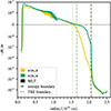 |
Fig. 5. Negative gradient of the mean entropy as a function of radius on a symmetric logarithmic scale. The entropy boundary is indicated with a vertical dashed line in the respective colour. The boundary of the TKE is indicated with a vertical dotted line in the respective colour. The formal Schwarzschild boundary of the initial stellar model computed using MLT is indicated with the dashed dark grey line. |
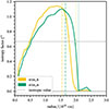 |
Fig. 6. Flow isotropy as a function of radius computed from the RANS data obtained from the sim_k and sim_m simulation in yellow and green, respectively. We indicate the entropy and TKE boundaries with dashed and dotted lines in the respective colour. |
At this point, we also point out that the convective flow in the simulations is not isotropic. Isotropic convection corresponds to ξ2 = 2/3. In the bulk of the convection zone we find ξ2 > 2/3, that is the flow is radially dominated. Similar results have for example been found in simulations by Andrassy et al. (2022), Kupka et al. (2018) or Viallet et al. (2013). This clearly shows that the isotropy assumption of the Kuhfuß model is not valid for convective cores.
4.2. Turbulent kinetic energy
In Fig. 7 we compare the model predictions of the TKE profiles with the results of the sim_k and sim_m simulation in the upper and lower panel, respectively. The same results are shown in Fig. E.1 on a logarithmic scale. For comparison, we show the results of the 1- and 3-equation model in each panel. The vertical lines indicate the different boundaries that we defined in Sect. 4.1. The TKE is not included in the MLT model itself, but can be easily computed based on the MLT velocity estimates if we assume an isotropic velocity field as in the Kuhfuß model. The TKE of the MLT model is then given by
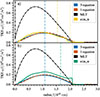 |
Fig. 7. Comparison of the TKE ω as a function of radius. Each panel shows the results obtained from the 1- and 3-equation model and from an MLT model with a blue, orange and black line respectively. The associated RANS correlations extracted from the sim_k and sim_m simulation are shown in the upper panel and lower panel, respectively. We indicate the entropy and TKE boundaries with dashed and dotted lines in the respective colour. |
 (20)
(20)
where uMLT denotes the convective velocity obtained from MLT. We show this profile as a black dash-dotted line in Fig. 7. This estimate for the TKE of the MLT exceeds the amplitude of the simulation results as well as the TKE from the Kuhfuß models by a factor of four. This is due to a difference in the dissipation length as was shown in A22. Therefore, we argue that the MLT does not provide a good estimate of the TKE for the given choice of the mixing length parameter α. We note that the values for α in the MLT and Kuhfuß models are obtained from separate solar calibrations.
Throughout the convection zone, the shape of the averaged TKE in the sim_k and sim_m simulation matches the predictions of the 1- and 3- equation models. The differences in the averaged TKE profiles in the sim_k and sim_m simulation can be largely attributed to the different initial thermal stratifications. The lower value of the entropy boundary in the sim_k simulation leads to a smaller value of the TKE boundary as compared to the sim_m simulation (see Table 1). This can be also seen in the flow field in Fig. 3, where a layer of waves is generated in the sim_k simulation beyond the entropy boundary. Similarly, this behaviour can be illustrated in the TKE profiles shown in Fig. 7. While in the sim_k simulation the TKE shows a step between the entropy and TKE boundary (coinciding with the generation of waves in this simulation), the TKE in the sim_m simulation reaches all the way to the Schwarzschild boundary where it drops sharply. Finally, the amplitude of the TKE is reduced in the sim_k simulation as compared to the sim_m simulation since the super-adiabatic region in the sim_k simulation is expanding. The growth is driven by the entrainment of high entropy material from the stable layer, which requires some kinetic energy. In contrast, the shrinking super-adiabatic region in the sim_m simulation uses less kinetic energy for entrainment. Here, this leads to the amplitude of the TKE of the sim_k simulation being in agreement with the predictions of the Kuhfuß model while the sim_m simulation exceeds these predictions. Towards the outer boundary of the simulation domain we observe another sharp rise in the TKE (see Fig. E.1). This is caused by the outer wall boundary condition. Since no energy is allowed to cross the boundary, the piled up thermal energy at the domain boundary gets converted into kinetic energy. We therefore do not consider the region with radius greater than 2.3 × 1010 cm in our conclusions.
The values for the TKE boundary depend strongly on the chosen definition (see for example discussion in Higl 2019; Higl et al. 2021). According to the definition laid out in Sect. 4.1, the region with significant TKE in the simulations is much less extended than in the stellar models. However, when defining the boundary as the point where the TKE decreased by a substantial fraction (of 10 to a 1000) as compared to the maximum, the TKE boundary is very comparable between simulations and stellar models (see Fig. E.1). While the TKE boundary in the Kuhfuß TCM can be changed by varying αω, the Schwarzschild boundary poses a lower limit for the convective core size, reached for a parameter value of αω = 0. Hence, for the former definition of the TKE boundary it would not be possible to tune αω to match the observations, while for the latter definition the simulations and stellar models are already in good agreement for the chosen parameter value. The TKE boundaries in the different simulations and stellar models are summarised in the fourth column of Table 1 in terms of radius, and in the fifth column in terms of fractional mass. For the MLT model, the TKE boundary coincides with the formal Schwarzschild boundary given in the third column because the nature of the model is local. Therefore, the values quoted in the fourth and fifth column refer to the chemically mixed core size in this case. By construction, the TKE of the 1- and 3-equation model have the same radial extent.
The excellent agreement between the TKE profiles and the model predictions indicates that the Kuhfuß model includes the most relevant physics in convective cores despite its wrong assumption about isotropy. The isotropy factors only seem to become important close to the convective boundary, where we see the largest deviations from the predictions. As the assumptions about the flow isotropy change the behaviour of the non-local terms, they are also expected to have a large impact on the overshooting distance (see K22). A simple solution to include anisotropy effects into the Kuhfuß model would be to include the profile of ξ into the equations. Since we see large differences in the ξ profiles of the sim_k and sim_m simulation (see Fig. 6), this approach does not seem desirable. It is also highly unlikely that different convection zones would lead to the same ξ profile. In order to include the effects of anisotropic flows properly into the Kuhfuß model, it is necessary to separate the radial from the total TKE equation. Other TCMs by Xiong et al. (1997), Li & Yang (2001) or Canuto (1992) already include this additional equation. We refer to Li & Yang (2007), Zhang & Li (2012a), Zhang (2016) for applications of these models discussing the role of the radial to the total TKE. We note, however, that the addition of equations into the implicit solver of a stellar evolution code is technically challenging.
4.3. Convective flux
In Fig. 8 we compare the model predictions of the convective flux variable Π with our simulation results. The model predictions for the 1- and 3-equation model as well as the MLT are almost identical in the bulk of the convection zone. The reason is that the convective flux variable, which represents the energy flux in the stellar model, is set by the energy source terms, since all energy needs to be transported to the surface of the star. The sim_m simulation matches the predictions in the bulk of the convection zone perfectly, while the sim_k simulation reproduces the same shape at an amplitude that is about 20% smaller than the predictions. This is in agreement with the results for the TKE where we found a lower TKE for the sim_k simulation because the super-adiabatic layer still expands. In a stellar model such a reduced convective flux would lead to a very different stellar structure. This can be excluded from an observational point of view.
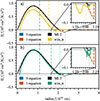 |
Fig. 8. Comparison of the convective flux variable Π as a function of radius. The results obtained from the 1- and 3-equation model and from the MLT model are shown with a blue, orange and black line respectively. The associated RANS correlations extracted from the sim_k and sim_m simulation are shown in the upper panel and lower panel, respectively. We indicate the entropy and TKE boundaries with dashed and dotted lines in the respective colour. |
The stellar model predictions differ at the convective boundary, where the Kuhfuß models show a region with negative convective flux (see inset of Fig. 8). The width and depth of the negative region is related to the region with the strongest braking of fluid motions and the consequent turnaround of plumes. In the MLT convective motions stop instantaneously at the Schwarzschild boundary without turning around. Hence Π does not show such a negative region in the MLT model. In A22, we show that the depth of the negative convective flux is related to the temperature stratification in the overshooting region (see also Eq. (13)). A large negative value of Π indicates that convection is still rather efficient in the overshooting region. The temperature gradient in that case is therefore close to the adiabatic one, which Zahn (1991) describes as a penetration layer. Small negative values indicate an inefficient convection with a temperature gradient close to the radiative one, which can also be seen by comparing Fig. 5 with Fig. 8. We use the ratio of the minimum to the maximum convective flux as an indicator for the convective efficiency in the negative buoyancy region (see Table 2). For the sim_m simulation we use the value of the minimum that is located slightly within the Schwarzschild boundary at about 2.03 × 1010 cm for our calculations. For the sim_k simulation we use the minimum located slightly within the TKE boundary at about 1.85 × 1010 cm. We find that the absolute value of the ratio of the 3-equation model is about one order of magnitude smaller than that of the 1-equation model. The measured ratios in the sim_k and sim_m simulation are smaller than for the 1-equation model and larger than the 3-equation model. Given the lack of thermal relaxation, we, however, cannot draw conclusions about the thermal stratification that would be reached after evolving the simulations over a thermal timescale.
Comparison of the negative convective flux region in the models and simulations.
We use the radial extent of the negative convective flux region as another criterion for a more quantitative comparison between the TCM and the simulations. For our comparison we use the full width at half maximum of the region with negative convective flux. We summarise the results in the fifth to seventh column of Table 2. As can be inferred already from Fig. 8, the radial extent of the negative convective flux is smaller in the 3-equation model than in the 1-equation model. In the sim_k simulation, the radial extent is similar to the value obtained for the 1-equation model. In the sim_m simulation, we observe a very narrow region of negative convective flux as the change in the temperature stratification acts as a stiff barrier and convective motions are braked in a very narrow region. For longer simulation times, the thermal stratification would adjust, also impacting the shape of this transition. Considering the short simulation times discussed here, we can however not draw any conclusions about this. In 1D stellar models a wider region of negative convective flux as in the sim_k simulation would lead to broader transition regions from the nearly adiabatic to the radiative temperature gradient.
Another important aspect of the temperature structure concerns the so-called Deardorff or counter-gradient layer (Deardorff 1966). This is a region in which the convective flux is still positive even though the entropy gradient is already positive (i.e. temperature gradient is subadiabatic). From a theoretical point of view, such a layer is expected because of the non-local term of the Φ equation. This term transports entropy fluctuations beyond the Schwarzschild boundary and acts as a non-local source of entropy fluctuations. The entropy fluctuations Φ then appear as a source in the Π equation. This layer has been observed in several simulations of stellar convection (Chan & Gigas 1992; Muthsam et al. 1995, 1999; Tremblay et al. 2015; Käpylä et al. 2017; Kupka et al. 2018) as well as other Reynolds stress models (Kupka 1999; Xiong & Deng 2001; Kupka & Montgomery 2002; Montgomery & Kupka 2004; Zhang & Li 2012b) and particularly in the 3-equation model (A22). Here, we investigate whether a Deardorff layer emerges in the 3D simulations of Sect. 3 as well. As mentioned before, the entropy boundary denoted by vertical dashed lines in Fig. 8 indicates the point where the sign of the entropy gradient changes and the stratification becomes subadiabatic. Figure 8 shows that the region of positive convective flux extends substantially beyond this entropy boundary in both simulation, that is a Deardorff layer emerges. It is especially important to note, that the initial model of the sim_m simulation did not have a Deardorff layer. It emerged naturally from the fluid dynamics simulation. The entropy boundaries in both simulations are still evolving during the simulation time, that is, the model is not fully thermally relaxed yet, explaining the differences between the sim_k and sim_m simulation. In order to make strong claims about the size and shape of the Deardorff layer, we would need to reach a thermally relaxed state, which is computationally not feasible at nominal stellar luminosity. Nevertheless, we can confirm the prediction of A22 that a TCM needs to include a convective flux and entropy fluctuation equation in order to improve the predictions of the temperature stratification, since Deardorff layers do not emerge in models without the non-local term in the entropy fluctuation equation. For further discussion of the physical relevance of the Deardorff layer we refer to Sect. 7.2.
4.4. Entropy fluctuations
The third equation of the Kuhfuß model computes the auto-correlation of entropy fluctuations, Φ. We show this quantity in Fig. 9. The profile of Φ is a strictly positive smooth function that is tightly correlated with the mean entropy gradient (see Fig. 5). We find a positive correlation between Φ and the entropy gradient in the superadiabatic regions and an anti-correlation in the subadiabatic regions. This is in contrast to the 3-equation model, which predicts a monotonically increasing Φ except for a small region around the entropy boundary. Around the TKE boundary both simulations show a peak in Φ similar to the 3-equation model. The amplitude of the peak that is located at or slightly above the TKE boundary, however, is two to three times larger in the simulations. Here, the sim_k simulation reproduces the overall shape of the peak better, probably because the thermal structure in the sim_k simulation and the 3-equation model is similar.
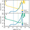 |
Fig. 9. Comparison of the squared entropy fluctuations Φ as a function of radius. The results from the 3-equation model are shown with a blue line. The associated RANS correlations extracted from the sim_k and sim_m simulation are shown in the upper panel and lower panel, respectively. We indicate the entropy and TKE boundaries with dashed and dotted lines in the respective colour. |
5. Analysis of individual terms
In Sect. 4 we compare the predictions for the three variables ω, Π, and Φ of the Kuhfuß model with our simulation results and found a general satisfactory agreement strengthening the usefulness of the Kuhfuß model. Within the Kuhfuß model, however, these unknowns are computed from terms that are individually modelled based on physical assumptions (see Sect. 2). Our 3D simulations offer the possibility to test these assumptions.
5.1. TKE equation
The TKE Equation (8) has three terms on the right-hand side, that originate from buoyancy contributions, non-local fluxes, and a model for viscous dissipation. The remaining terms of the full RANS Equation (5) are neglected. In order to quantify the contribution CXj(r) of each term Xj to the left-hand side of Eq. (5), we compare the absolute magnitudes of each term |Xj(r)| and normalize them as
 (21)
(21)
where we sum over all terms Xi(r) on the right-hand side of Eq. (5). We then integrate CXj(r) over the convective zone to find the total contribution fraction CXj,
 (22)
(22)
where Δr = r1 − r0 and r0, and r1 are the inner radius of the simulation domain and the TKE boundary, respectively. We give CXj of the TKE equation in the first column of Table 3. A visualisation of the radial dependency of CXj(r) can be found in Appendix F.
Contributions of (absolute) individual terms to the total lhs.
Within the Kuhfuß model, the non-local flux term is responsible for setting the size of the convective core (see Ahlborn 2022). In our simulations, we find that it accounts for about 30% of the right-hand side of the TKE equation and dominates towards the TKE boundary (see Fig. F.1). In Fig. 10 we compare the Kuhfuß 1- and 3-equation models, which compute the non-local flux in the downgradient approximation (see Eq. (8)), to the RANS averaged values of the sim_k and sim_m simulation in the upper and lower panel, respectively. To compare consistently with the Kuhfuß model, we transform the non-local term of Eq. (5) using the anelastic approximation (Ogura & Phillips 1962; Gough 1969) into
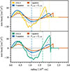 |
Fig. 10. Comparison of the non-local terms of the TKE equation. The results obtained from the 1- and 3-equation model are shown with a blue and orange line, respectively. The associated RANS correlations extracted from the sim_k and sim_m simulation are shown in the upper panel and lower panel, respectively. We indicate the entropy and TKE boundaries with dashed and dotted lines in the respective colour. |
 (23)
(23)
All curves in Fig. 10 reproduce the same wave-like shape with negative non-local flux contributions in the middle of the convection zone and positive contributions close to the stellar centre and convective boundary. The radial positions of the sign changes in the simulation roughly matches the 1D models. In the stable layer, the non-local flux quickly approaches zero. This indicates that the Kuhfuß solution for the non-local flux contains all relevant physics. The two simulations only differ in the radial position of the transition towards the stable layer and the magnitude of the non-local flux around the convective boundary. This could indicate that some of the parameters of the Kuhfuß model need to be tuned differently. Given the evolving thermal stratification, calibrating the parameters of the convection model, however, remains difficult. Another solution to the mismatch could be the inclusion of flow anisotropy into the model (see Sect. 8.1).
The buoyancy term as given in Eq. (5) is expected to dominate the dynamics of (nearly) incompressible flows like stellar core convection (see left column of Table 3). In the Kuhfuß model it is modelled by the Boussinesq approximation, which directly connects the buoyancy flux to the convective flux variable Π (see first term in Eq. (8)). Even though we do not use this approximation for our RANS analysis, we find that the agreement between the sim_m simulation and the 1D models is excellent (see Fig. G.1 in the appendix). The result of the sim_k simulation is slightly rescaled compared to the 1D models, but the overall shape agrees quite well. Therefore, we argue that the Boussinesq approximation is well justified for this term. Moreover, the shape of the curves in Fig. G.1 is almost identical to Fig. 8 and hence the discussion of the features around the convective boundary is analogous to the discussion of Π.
In addition to the gradient of the mean pressure a second component, involving the pressure fluctuations, shows up in Eq. (5). In Fig. 11 we show these buoyancy pressure fluctuations computed from the simulations. There are two things that we can immediately take away from this figure: (i) while this term is neglected in the Kuhfuß model, our results show that, integrated over the whole convective zone, it actually has a substantial contribution to the total TKE (see Table 3), (ii) its shape is very similar to the non-local term, but with opposite sign (see dashed lines in Fig. 11). We discuss in the following why this similarity is expected. In the TKE equation it is only the flux contribution of the pressure fluctuation term that remains,
(e.g. Canuto 1992). To account for this term, Lumley (1978) suggested the following closure  and a = 1/5 making the pressure fluctuations proportional to the third-order moment of velocity such that
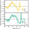 |
Fig. 11. Pressure fluctuation term and non-local term of the 3D simulations as a function of radius. The results of the sim_k and sim_m simulation are shown in the upper and lower panel, respectively. The non-local term is scaled with a factor of −2/5 to demonstrate the quality of the closure for the pressure-fluctuation term. We indicate the entropy and TKE boundaries with dashed and dotted lines in the respective colour. |
Given this closure, the flux component of the pressure fluctuation term and the non-local term have the same functional form. In Fig. 11 we also show the non-local term scaled with this factor of −2a and find a very good agreement, highlighting the quality of this closure. When implicitly solving for the model equations of the 3-equation model, the action of the pressure fluctuation term can be hence absorbed by the non-local term. To make the model more general one would only need to change the definition of the non-local parameter αω to account for the reduction through the pressure fluctuations. For the comparison with the 1- and 3-equation model, this also implies that we need to compare the 1D result to the sum of the non-local and pressure fluctuation term from the simulations. This is shown with the grey lines in Fig. 10. Clearly, the discrepancy between the 1D and 3D results decreases, however, without achieving a complete agreement.
The Kuhfuß model also contains another term in the TKE Equation (8), which describes the dissipation of kinetic energy based on the Kolmogorov scaling of isotropic turbulence. Our 3D simulations do not contain an explicit dissipation term as discussed in Sect. 3.2. The only source of dissipation is of numerical nature. Hence, we cannot extract it directly from the simulation data. However, we can estimate the numerical dissipation by comparing the left-hand side of Eq. (5) to the terms on the right-hand side. In Fig. 12 we see that the residual of the TKE equation as extracted from the simulations has a similar amplitude as the 1D dissipation models. Even though the TKE in the simulation is ultimately dissipated by numerical viscosity, the dissipation in ILES simulations follows a Kolmogorov turbulent cascade (Aspden et al. 2009). Recently, Andrassy et al. (2022) showed that SLH and similar codes have a TKE spectrum that follows the Kolmogorov scaling (see also Cristini et al. 2019; Blouin et al. 2023). As the dissipation term of the Kuhfuß model is also based on the assumption of a turbulent cascade, this explains the agreement between the simulation and the TCM.
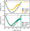 |
Fig. 12. Residual term of the 3D simulations as a function of radius. The results of the sim_k and sim_m simulation are shown in the upper and lower panel, respectively. For comparison, we show the dissipation term from the 1- and 3-equation model with an orange and blue line, respectively. We indicate the entropy and TKE boundaries with dashed and dotted lines in the respective colour. |
Equation (5) contains two more terms that are neglected in the Kuhfuß model. The first is a viscous flux term, which we cannot extract from the simulations because our simulations lack an explicit viscosity. It is contained in the residual term shown in Fig. 12, which has already been discussed. The other neglected term is the shear term, which we can easily measure in the simulations. However, when we integrate its contributions to the TKE over the convective zone, we find that it accounts for less than 1% of the right-hand side of the TKE equation. The simulations therefore confirm that this term can be neglected. The extracted profiles of the neglected terms can be found in the appendix (see Fig. G.2).
5.2. Convective flux equation
In the 3-equation Kuhfuß model the convective flux variable Π is computed by Eq. (9), with the terms on the right-hand side being associated with buoyancy, potential energy, radiative energy transport, and a non-local turbulent flux of entropy fluctuations. Compared with the full RANS Equation (6), the Kuhfuß model therefore neglects terms describing viscous, shear, pressure fluctuation, and nuclear energy effects. We give the integrated contributions of each term to the right-hand side of the convective flux equation in the second column of Table 3. The different contributions as a function of radius are shown in Fig. F.2. As described in Sect. 2.3, the 1-equation model assumes a proportionality between Π and the entropy gradient, which makes Π trivial to compute. Therefore, the 1-equation model does not provide predictions for the terms in Eq. (6). The same applies to the MLT.
In Fig. 13, we compare the radial dependence of the non-local term in the 3-equation model and our 3D simulations. All curves show the same general shape with similar magnitudes. Both simulations show a steep drop close to the TKE boundary. Comparing Fig. 13 with Fig. 8, we find that the steep drop in the non-local flux of Π is located at the same position as the regions with negative values for Π. A similar feature can be found in the 3-equation model, which shows a region with small negative non-local fluxes close to the TKE boundary (see inlet of Fig. 13), corresponding to the radial position of negative Π in Fig. 8. We therefore associate this feature with the ballistic overshooting picture, where convective plumes are breaking and turning around as a result of buoyancy. We conclude that the Kuhfuß model describes all relevant physics of this term correctly, but some parameters still need to be calibrated precisely. To test the dependence of these parameters on the characteristics of individual convection zones, more 3D simulations will be needed. As for the non-local term of the TKE equation, the inclusion of the flow anisotropy is expected to have an impact.
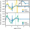 |
Fig. 13. Comparison of the non-local term of the convective flux equation Eq. (6) as a function of radius. The results for the sim_k and sim_m simulation are shown in the upper and lower panel, respectively. The results of the 3-equation model are shown with the blue line. We indicate the entropy and TKE boundaries with dashed and dotted lines in the respective colour. |
The buoyancy term is another important term for the Π equation. Its profile, which accounts for approximately 30% of the right-hand side of Eq. (6), is given in Fig. 14. Close to the TKE boundary, we observe that the buoyancy term turns negative. We attribute these negative values of the buoyancy term to the fact that some terms, especially when related to the thermal stratification, are still evolving over the simulation timescale. Hence, the final average integrated over the whole simulation time is different from the local average of individual snapshots. This can lead to negative values when using the time integrated average, even though results may be still strictly positive when using the local averages.
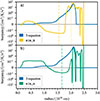
The term describing the potential energy is proportional to the gradient of entropy (see Eq. (6)). Therefore, we see a sign change at the entropy boundary in Fig. 15. In the 3-equation model the sign change is located much closer to the stellar centre. This shows that the temperature stratification in the simulations has significantly evolved compared to the initial state, which indicates that the Kuhfuß model does not provide a fully consistent temperature stratification (the initial stratifications are shown in Fig. 1). However, the 3D simulations are also not able to provide the exact temperature stratification, since they are not in thermal equilibrium yet. Both simulations are still affected by their initial temperature stratification, as can be seen by the fact that the sign change in the sim_k and sim_m simulation is located at different radii. The magnitude of the potential term is similar in the sim_k and sim_m simulation, but the 3-equation model predicts much smaller amplitudes. An increased superadiabaticity in the 1D model would reduce this discrepancy. The discrepancies towards the TKE boundary between the 3D data and the Kuhfuß model arise from the differences in the thermal stratification and the TKE, both entering the potential term of the convective flux equation, which are more pronounced in this region. The simulations also show a sign change close to the stellar centre in Fig. 15. We argue that this is a boundary effect of the simulation setup.
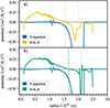
The Kuhfuß model neglects some contributions to Eq. (6). These are shown in Fig. G.4. Analysing the sim_k and sim_m simulation, we find that the shear term and the nuclear energy term can safely be neglected, since they only contribute 7 × 10⁻⁶ and 1 × 10⁻⁴% to the right-hand side of Eq. (6), respectively. From the sim_k and sim_m simulation, we can estimate the viscous contributions by computing the difference of the right and left-hand side terms of Eq. (6) (see Fig. G.5). We find that the amplitude of the residual terms is comparable to the buoyancy term. Similar to the TKE, the convective flux is transferred to smaller and smaller scales on a turbulent cascade before it is eventually dissipated by viscosity. This leads to the large values of the dissipation term, counter balancing the sources of the convective flux equation. Different dissipation models need to be explored to account for such effects in the TCM (e.g. Canuto & Dubovikov 1998). Furthermore, the Kuhfuß model also neglects the pressure fluctuation term in Eq. (6). Similar to the TKE equation, we find that this is an oversimplification, since pressure fluctuations created by buoyant flows do contribute to the dynamics of the flow. The integrated contribution of the pressure fluctuation term is 37.6%.
The radiative dissipation terms found in the sim_k and sim_m simulation show an integrated contribution of 2 × 10⁻³%. In comparison, the prediction of the 3-equation model is about four orders of magnitude smaller than the simulation result, and does also show a different functional form (see Fig. G.3). Despite this discrepancy, the term is not expected to have a substantial impact on the behaviour of the convective flux equation because its magnitude in the 3D simulations and the 1D models is negligible. Different models for the dissipation term, which consider the complete second-order derivatives as suggested by Canuto (1992) and Canuto & Dubovikov (1998) might be able to reduce the discrepancy that was found between the 1D and 3D results.
5.3. Entropy fluctuation equation
Finally, we use our simulations to analyse the terms in Eq. (7), which describes the entropy fluctuations Φ. The different contributions as a function of radius for the Φ equation are shown in Fig. F.3. The corresponding counterpart in the 3-equation Kuhfuß model is Eq. (10). The 1-equation Kuhfuß model as well as the MLT do not make predictions about the entropy fluctuation profile. Therefore, we cannot compare the simulation results to these models.
The predicted and measured profiles of the non-local term are shown in Fig. 16. In contrast to the non-local terms of the TKE and Π-equations, we find significant differences in both shape and magnitude between the simulations and the Kuhfuß model. On the one hand, the Kuhfuß model predicts that the non-local term of Φ is strictly positive throughout the bulk of the convective region. Furthermore, the 1D model shows a large negative peak around the TKE boundary. The simulations, on the other hand, find a similar shape as the previous non-local terms, that is two mainly positive regions in the very centre and close to the TKE boundary in combination with mainly negative fluctuations in the bulk of the convective region. Moreover, the peak around the TKE boundary is about one order of magnitude smaller than in the 3-equation model. This indicates that the parameters of this term need to be recalibrated.
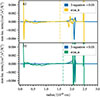
The potential term accounts for 66.9% of the absolute contributions to the right-hand-side of Eq. (7) implying that the superadiabaticity is still the dominant source of entropy fluctuations. The shape of the potential term of the entropy fluctuations in the Kuhfuß model and in the 3D simulations is similar to the potential term of the convective flux equation (compare Figs. 17 and 15). The discussion for the bulk of the convective zone is therefore analogous to the potential term in Sect. 5.2. The discrepancies between the 3D data and the Kuhfuß models between entropy and TKE boundary arise from the differences in the thermal stratification and the convective flux Π that enter the potential term of the entropy fluctuation equation.
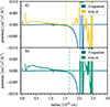
The discussion of the radiative loss term follows that of the convective flux equation (see Fig. G.6). Overall, the contribution of the term is negligibly small, but the simulations find losses with amplitudes five orders of magnitude larger than in the Kuhfuß model. This indicates that the model of radiative losses in Eq. (10) is largely oversimplified, but the effect of an updated term is expected to be negligible. The Kuhfuß model neglects terms related to nuclear energy generation as well as viscosity effect. The neglected terms are shown in Fig. G.7. The former one is negligible, as we find a total integrated contribution of only 9 × 10⁻⁴%. As for the other two equations, we attempt to probe the viscosity effects by looking at the residuals of Eq. (7). We find that the residual is on the order of the potential term and currently not accounted for in the TCM (see Fig. G.8). As for the convective flux equation additional dissipation terms need to be explored. We note however that we do not give any quantitive estimates of these dissipation terms because the statistical fluctuations in the Φ equation are stronger.
6. Parameter variations
The approximation of different physical effects in convection models simplifies the problem at hand at the price of introducing adjustable parameters. These parameters need to be chosen appropriately to ensure the physical accuracy of the convection model solutions. In MLT, the mixing length parameter is left as the only adjustable parameter comprising all physical effects. In most implementations, other parameters take fixed values and as such remain hidden (e.g. Böhm-Vitense 1958; Kippenhahn et al. 2012). In the local and time-independent limit, the Kuhfuß 1- and 3-equation model collapse back to the MLT when choosing appropriate parameter values and therefore also depend already on the hidden parameters in MLT, which differ between different implementations, for example between the widely used Weiss et al. (2004) and the Böhm-Vitense (1958) MLT. The parameter values calibrated to the Böhm-Vitense (1958) MLT are used as default values, as we discuss in Sect. 2.2. Unlike in most implementations and applications of MLT, here we do not only vary the most important parameter of the convection theory (i.e. the dissipation-length parameter, parametrising the dissipation of TKE) but also test the impact of parameters describing other physical effects in the Kuhfuß model.
These closure relations mean that the 3-equation model is left with a number of model parameters. The parameters αω and CD describe the non-local term and the dissipation rate of the TKE equation (Eqs. (8) and (11)). The non-local terms of the convective flux and entropy fluctuation equations contain two additional parameters αΠ and αΦ (Eq. (11)). Additionally, γR (Eq. (12)) parametrises radiative losses and c4 describes the newly introduced dissipation mechanism as described in Sect. 2.2. Lastly, the dissipation length scale Λ is described by the dissipation length parameter α and the parameter βs from the Wuchterl (1995) correction (Eq. (14)). We keep the constants c2 and c3 appearing in βs fixed for this analysis. In Sect. 5 we show that the radiative dissipation term in the simulations and the Kuhfuß model remains negligibly small. An impact of this parameter would therefore only be noted for large changes in its value and hence we keep it fixed at its default value for this analysis as well.
A key advantage of the 3-equation model is its ability to predict the thermal structure of convective zones. Hence, we now explore the behaviour of the potential term of the convective flux equation in Fig. 18, which is proportional to the thermal stratification (Eq. (6)). The results for varying the non-local parameters αω, αΠ, and αΦ are shown in the upper, middle, and lower panel, respectively. While a similar analysis would be possible for the entropy fluctuation equation, we refrain from this analysis because the relative statistical fluctuations in the different terms of this equation are stronger. The results of the sim_k and sim_m simulation are shown for comparison. The only notable change of the potential term when varying the parameter αω concerns the radial extent of the close to adiabatic regime which follows the change of the TKE boundary discussed previously. For the potential term the region with superadiabatic and close to adiabatic values increases for increased parameter values. However, αω cannot be increased arbitrarily as this will lead to unrealistically large convectively mixed cores.
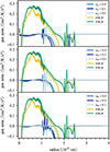 |
Fig. 18. Comparison of potential terms of the convective flux equation of the 3-equation model as a function of radius. The results of the sim_k and sim_m simulation are shown with a yellow and green line, respectively. The potential terms of the convective flux equation obtained from the 3-equation model are shown with the remaining coloured lines (see legend for details). The parameters αω, αΠ and αΦ are varied in the upper, middle and lower panel respectively. The mid-blue line indicates the default parameter values. |
For larger parameter values of αΠ the agreement with the simulations can be improved by increasing the magnitude of the potential term following the increase of the superadiabaticity (see middle panel of Fig. 18). This increase of the superadiabaticity occurs as the potential term needs to counteract the smaller values of the non-local term in the centre of the convection zone that occur for larger values of αΠ. It is however not possible to reach the magnitude of the potential term as found in the simulations.
Finally, αΦ parametrises the non-local term of the Φ-equation. As discussed previously this term is responsible for the occurrence of the Deardorff layer. For decreasing values of this parameter, the non-local transport of entropy fluctuations decreases and hence one would expect the extent of the Deardorff layer to decrease until it vanishes for αΦ = 0. In the lower panel of Fig. 18, we observe this behaviour as the close to adiabatic region increases in size (i.e. decreasing the extent of the Deardorff layer) for decreasing values of αΦ.
The parameters of the 3-equation model have their largest impact on the convective flux variable in the overshooting region. In the bulk of the convection zone, the impact of the parameters is mostly negligible. This weak dependence of the convective flux variable on the model parameters means that the behaviour of the TKE equation to changing αω and CD is very similar in the 1-equation model and the 3-equation model. Increasing CD increases the dissipation rate of the TKE, leading to a smaller magnitude and a TKE boundary located at smaller radii. Because of the dissipation mechanism in the 3-equation model, however, which includes the effects of buoyancy waves, the effect of changing CD is partially cancelled (Sect. 3 of A22). Increasing αω leads to a larger non-local term, transporting more TKE beyond the Schwarzschild boundary, moving the location of the TKE boundary further out in radius. As the non-local term is negative in the bulk of the convection zone, the magnitude of the TKE decreases with increasing αω. We further note that changing αΠ and αΦ does not change the convective core size notably as has been already shown in A22. There is hence some margin in changing αΠ and αΦ to reproduce the thermal structure of the simulation without substantially modifying the properties of the TKE in the 3-equation model. Finally, the strength of the dissipation mechanism introduced in A22 is parametrised by c4. Changing c4 mainly impacts the location of the TKE boundary without changing the TKE magnitude. Therefore, c4 can be kept at its default value.
In Sect. 4 we discuss that the TKE boundaries in the sim_k and sim_m simulation are located further inwards than predicted by the Kuhfuß 1- and 3-equation model. More specifically, the TKE of the simulations does not extend beyond the formal Schwarzschild boundary of the initial stellar models (see Table 1). In the Kuhfuß models, the formal Schwarzschild boundary is the lower limit of the convective core size, obtained for a parameter value of αω = 0. This can be ruled out by observations, as convective overshooting beyond the formal Schwarzschild boundary is expected for the type of star considered here, requiring αω > 0. This behaviour prevents us from calibrating the parameter αω to the 3D simulations. A final conclusion on the location of the TKE boundary remains difficult, however, as the thermal structure of the simulations is still evolving on the simulation timescale.
7. Discussion
The two simulations we discuss in this work show substantial differences in the size of the turbulent convective region (see Sect. 4 and in Table 1). As we used the same code and numerical setup, this result might occur as surprising at first. In the following, we discuss the robustness of our results in the bulk and the boundary of the convective region and also with regard to other potential uncertainties.
The only difference between the two simulations is the stellar model used to initialise the simulations–for the sim_k simulation we used a Kuhfuß 3-equation model, while for the sim_m simulation we used an MLT model with ad hoc overshooting. These initial models were selected to have the same central hydrogen abundance and chemically homogeneous core size. Because of these choices, the most important remaining difference between the two initial models is the thermal stratification (see Fig. 1). We therefore conclude that the observed differences in the location of the TKE boundary between the sim_k and sim_m simulation originate from the different initial thermal stratifications. We note that even though the temperature stratification evolves self-consistently in the hydrodynamic simulations, the thermal adjustment time is much longer than our current simulation time. For the Kelvin–Helmholtz timescale at the Schwarzschild boundary we find approximately 2.5 × 10⁵ years, which is many orders of magnitude larger than the approximately one year of simulation time that we discuss here.
This dependence of the simulation results on the initial stellar models means that we need to understand the aspects of the simulation that can be compared and the aspects that need to be interpreted with some more care.
7.1. Bulk convective region
The comparison of the superadiabaticity in the two simulations in Fig. 1, shows that in the bulk of the convective region both simulations reached qualitatively and quantitatively a very similar thermal stratification. The superadiabaticity is also in good qualitative agreement with the one found in the thermally relaxed simulations of Andrassy et al. (2024) (see their Figs. 7 and 8). As we discuss in Sect. 3.3 and Appendix D, the two simulations reached a dynamically converged state given the thermal stratification. Taking these points together, we conclude that results obtained in the bulk of the convection zone and quantities evolving on a dynamical timescale are robust. This allows us to compare the properties of the simulation and the 1D model that are related to the flow dynamics in the bulk of the convection zone. Notwithstanding, the adjustment of the thermal stratification does also leave imprints in the bulk convective region. One indicator for this is that the sim_m simulation shows both a larger convective flux and TKE than the sim_k simulation. We attribute this reduced flux and TKE in the sim_k simulation to the adjustment of the thermal stratification in the convective boundary region in this simulation, where energy is still required to establish a nearly adiabatic stratification.
7.2. Convective boundary region
As mentioned previously, the simulations did not reach a thermal equilibrium yet. The still evolving thermal stratification and the comparably short simulation time mean that we cannot draw quantitative conclusions about the convective boundary region, for example the extent of the convective core in a real star, as it has been shown that the adjustment of the convective core size takes a substantial fraction of the thermal timescale (e.g. Käpylä 2019; Baraffe et al. 2023; Andrassy et al. 2024). This circumstance must be taken into account when interpreting all results. However, the thermal profiles of both simulations show features that support the conclusion that they are approaching the thermally relaxed state in a self-similar fashion. In both simulations, a Deardorff zone emerged, that is, a region with positive convective flux in conjunction with a subadiabatic stratification, even though the initial MLT 1D stellar model did not show this feature. The radial location of the entropy boundary does approximately agree between both simulations, followed by a Deardorff layer of approximately the same extent. Such a Deardorff layer is a feature that is commonly observed in 3D simulations of convection, (e.g. Käpylä 2019, 2021, 2024) and in the thermally relaxed simulations of core hydrogen burning by Andrassy et al. (2024). Finally, in the superadiabaticity profiles of the sim_k simulation (see lower left panel of Fig. D.1) it can be observed how convection evolves towards an almost adiabatic Deardorff and overshooting zone, as one would expect for the conditions studied here. We hence conclude that we can draw qualitative conclusions about some of the important features of the thermal stratification, while quantitative conclusions are beyond reach given the lack of thermal relaxation.
Given these preliminaries, we can use the discrepant structure between the sim_k and sim_m simulation and the 1D Kuhfuß models to draw conclusions about potential shortcomings of the TCM and what the initial thermal stratification should look like. If the TCM accurately described the physics and predicted a consistent thermal and velocity structure, one would expect the stellar models to reproduce the velocities observed in the simulations. However, for both simulations we observe the thermal structure evolving away from the initial thermal stratification. We find that the entropy boundary–defined as the sign change of the entropy gradient–moved outwards in the sim_k simulation and moved inwards in the sim_m simulation compared to the initial stellar models (see Fig. 5). This indicates that the initial temperature structure predicted by the stellar models is inconsistent with the predicted velocity profiles. We hence conclude that the physics describing the thermal stratification in the TCM is incomplete and needs to be improved.
The impact of the initial thermal structure can be also observed as changes in the behaviour of some of the equation terms for radii greater than 2.05 × 1010 cm, which corresponds to the formal Schwarzschild boundary in the initial models (see Table 1). We associate the change in behaviour with the waves that start travelling beyond the formal Schwarzschild boundary. As our simulations are focussed on the convection in the core, we do not resolve the waves travelling in the stably stratified region. This leads to the presence of TKE in this region. The more abrupt transition of the temperature gradient in the MLT model as compared to the 3-equation model leads to an imprint in some of the simulation terms, for example the gradient of the mean entropy and related terms, the buoyancy term of the convective flux equation, and the squared entropy fluctuations Φ.
As noted above, the simulations have not yet reached a consistent thermal and velocity structure. To evolve into a stationary and consistent configuration of these two quantities longer simulation times, on the order of the thermal timescale, are needed. A potential approach to reach consistent convective structures is suggested in Higl et al. (2021), in which initial stellar models with varying parameters (e.g. the overshooting extent) were used. In the same direction, Anders et al. (2022) suggest to iteratively change the thermal structure of the simulations to accelerate the computations. They bridge larger than the dynamical time step by extrapolating the current thermal structure of the simulation and reinitialising the simulation with the extrapolated structure. In the 3-equation model, the parameters αΠ and αΦ may be varied to change the thermal structure of the stellar model and eventually match the entropy structure of the simulations.
7.3. Further uncertainties
When discussing the extent of the convective region, we have to further take into account that the position of the convective boundary depends on the definition used to compute it. In the two simulations discussed above, the horizontal component of the TKE shows non-zero values further out than the radial component. If we used this horizontal component to estimate the convective core size of the sim_k simulation, we would obtain a larger value in comparison to the estimation from the isotropy profile (which is computed as the ratio of the radial to the total TKE). Similarly, the TKE in the wave dominated region, that is beyond the TKE boundary, has a similar profile as in the Kuhfuß models (compare the location of the TKE minimum in the upper and lower panel of Fig. E.1 with the extent of the orange and blue lines). As these waves remain unresolved in our simulations, the significance of this result remains unclear. Furthermore, given the flow pattern (see Fig. 3) and the different spatial components of the TKE, we conclude that the horizontal component of the TKE observed beyond the TKE boundary most likely has a different origin than convection (e.g. internal gravity waves). Finally, the behaviour of the individual equation terms, for example the region in which they show non-zero values, further supports the choice of the TKE boundary based on the isotropy profile. For example, the non-local terms of the TKE and the convective flux equation vanish at the TKE boundary.
Finally, we note that the RANS data analysed in this work still show statistical fluctuations as a result of the relatively short computation time of five convective turnovers. In some cases, these statistical fluctuations surpass the sensitivity of the convection model to changing the model parameters. Hence, calibrating exact model parameters remains difficult for the current simulations, and we only discussed the dependence of individual terms on variations of the model parameters. For longer simulation times, we expect the statistical fluctuations to decrease and improve the ability to calibrate the model parameters. In case it remains impossible to calibrate model parameter for longer simulation times, this is indicative of more fundamental shortcomings of the convection model. This behaviour can be exemplified for the potential term of the convective flux equation which cannot be matched with the simulations for varying αΠ and αΦ. This discrepancy can potentially be attributed to missing physics describing the thermal stratification like the pressure fluctuation term in the convective flux equation. To reach a final conclusion, longer simulation times are needed.
8. Conclusion
We compare the convective core properties predicted by the Kuhfuß TCM (Kuhfuß 1987; Kupka et al. 2022; Ahlborn et al. 2022) to 3D hydrodynamic simulations. To compute the hydrodynamic simulations, we used the finite-volume code SLH, which solves the inviscid Euler equations. To compare the simulations to the TCM, we used the RANS analysis, which is an ideal tool for testing the physics of convection models and for paving the way for improving them. The RANS analysis of the simulations shows that the TCM in its current formulation describes the physics of convection most relevant for stars accurately. In the following, we summarise our findings for the three equations of the TCM we used.
8.1. TKE equation
For stellar models with convectively burning cores, the TKE is the most important convective variable because it is used to determine the chemical mixing induced by convection (see Eq. (15)). The TKE extracted from the sim_k and sim_m simulation, which differ in the initial 1D stellar model, agrees well with the 1- and 3-equation model in terms of the magnitude (see Fig. 7). The prediction for the TKE computed by MLT in contrast seems to be overestimated. For the radial extent of the convective core, we obtain two different values from the sim_k and sim_m simulation. This discrepancy can be related to the difference in the thermal structure, which still adjusts on the simulation timescale. This behaviour implies that the simulations were not initialised with the correct thermal equilibrium structure, which indicates that the underlying stellar models need to be improved. When we compare the TKE boundaries obtained from the isotropy profile to the entropy boundaries obtained from the entropy gradient, we find an extension of the TKE into the subadiabtic region. This shows that an overshooting zone in the classical sense emerges. We note, however, that the radii of the TKE boundaries of the sim_k and sim_m simulation are smaller than predicted by the Kuhfuß models. At this point, we cannot conclude whether the TKE extent obtained from the 1- and 3-equation model is really discrepant with the TKE boundaries from the simulations because they are prone to the systematic uncertainties described above. To obtain a more reliable estimate of the radial TKE extent, much longer simulation times are required to allow for stationary thermal and TKE profiles.
In the TCM, individual physical effects are parametrised by different terms, which is an important difference compared to the MLT. The comparison of the different terms of the TKE equation as predicted by the 3-equation model with the two hydrodynamic simulations shows an overall agreement of the buoyancy, dissipation, and non-local term. As in the MLT, the buoyancy term is an important source of convective motions in the TCM. The comparison of Figs. G.1 and 8 shows that the buoyancy term of the TKE (ω) equation computed from velocity perturbations, density, and the gradient of the mean pressure (see Eq. (5)) is consistent with the profile of the convective flux variable Π, both extracted from the hydrodynamic simulations. We therefore conclude that the Boussinesq approximation provides a good approximation to the buoyancy term of the TKE equation. Based on the current thermal stratification, the simulations seem to favour the smooth decrease in the non-local term towards the TKE boundary, as seen in the 3-equation model, instead of the steep cut-off in the 1-equation model. This is also supported by the shallower region of negative convective flux found in the simulations. This might change when a thermally relaxed structure is reached, however. Terms that are neglected in the 3-equation model have a negligible magnitude in the simulations, and the only exception is the pressure fluctuation term. For this term, we find a non-negligible magnitude in the convection zone. In turbulent flows, different processes generate pressure fluctuations, with the acceleration by pressure gradient forces (i.e. buoyancy) being the most important process under stellar conditions (e.g. Sander 1998; Viallet et al. 2013, for a further discussion of the pressure fluctuation terms we refer to Launder & Reece 1975; Lumley 1978; Pope 2000). As a result of the buoyant driving of the process, the magnitude of the pressure fluctuations is not negligible. Close to the convective boundary, the compression or contraction of buoyantly rising and sinking material might also generate pressure fluctuations and might thus enhance the pressure fluctuation term. To capture all relevant physics of the TKE, a TCM needs to incorporate the pressure fluctuation term. Following the closure of Lumley (1978) for the flux component of the pressure fluctuation term, the non-local term implicitly absorbs the effects of the pressure fluctuations. To include this component of the pressure fluctuation term in the TCM in a more general way, the definition of the non-local parameter αω would need to be changed and a separate parameter would need to be introduced for the closure of the pressure fluctuation term. We therefore conclude that the TKE equation of the 3-equation model is already a quite accurate representation of the processes in a real star.
In contrast to the 1D Kuhfuß models, the 3D simulations allow us to investigate the spatial distribution of the TKE. In both simulations, we find that the TKE is dominated by radial motions in the bulk of the convection zone but becomes dominated by horizontal motions towards the TKE boundary. This confirms the results from other simulations (e.g. Viallet et al. 2013; Cai 2020; Andrassy et al. 2022) or in a four-equation Reynolds stress model (Li & Yang 2007). Following other Reynolds stress models (Li & Yang 2001, 2007; Xiong 1979; Canuto 1992; Canuto & Dubovikov 1998), a fourth equation might be introduced in the Kuhfuß model to describe the vertical component of the TKE by computing a self-consistent solution of the spatial TKE distribution. In contrast, the introduction of an isotropy profile, for example obtained from 3D simulations, is not desirable because the overshooting distance strongly depends on this profile. We further note that for a different object, a different profile might be obtained, as described by Kupka et al. (2018) for simulations of a white dwarf.
8.2. Convective flux equation
As described before, a theory of convection is needed in stellar structure and evolution models to compute the energy flux and in turn the temperature gradient in convective regions. Globally, the convective flux variable obtained from the simulations and the Kuhfuß models agree well. As in the Kuhfuß models, we find a layer of negative convective flux in our simulations towards the TKE boundary. We note, however, that the depth and radial extent of this region are reproduced neither by the 1- nor the 3-equation model. The comparison of the negative convective flux region between the simulations and the Kuhfuß model indicates a temperature gradient somewhere in between the 1- and 3-equation model. As noted before, this depends on the thermally relaxed structure, which has not been reached in our simulations so far.
The comparison of the convective flux and the entropy gradient shows that a Deardorff layer (i.e. a layer with a positive convective flux and subadiabatic temperature stratification) emerges in both simulations, independently of the initial thermal stratification. From this, we conclude that the temperature stratification in the convection zone and especially around the convective boundary is not as simple as predicted by MLT or the 1-equation model. A Deardorff layer was found in a variety of different setups (Brandenburg 2016; Käpylä et al. 2017; Käpylä 2019; Blouin et al. 2023; Andrassy et al. 2024). This implies that a realistic convection model should predict the existence of a Deardorff layer, as demonstrated for the 3-equation model. In comparison to the 3-equation model, the sim_k simulation suggests that the TCM underestimates the radial extent of the superadiabatic region. In the 3-equation model, the radial extent of the superadiabatic region is influenced by the non-local parameters αΠ and αΦ. We point out that the occurrence of numerical noise in some terms of the 3-equation model prevented us from achieving the parameter values required to match the simulation results (see Sect. 6). The radial extent over which the temperature gradient transitions from the nearly adiabatic to the radiative value remains inconclusive because the simulation time is much shorter than the thermal timescale. We envisage using the 1-equation model as an initial model for the simulations as a useful future extension of this work. In the 1-equation model, the overshooting zone has a close to adiabatic temperature gradient that might be closer to the expected equilibrium stratification. This would allow us to reach more conclusive results.
For the terms of the equation describing the convective flux variable Π, the comparison between the simulation and the TCM becomes more difficult because of the stronger statistical fluctuations. We find a broad agreement for the non-local term and the potential term, however. Comparable to the entropy fluctuation variable Φ, the buoyancy term of the Π equation from the simulations reproduces the global trends of the Kuhfuß model without being in perfect agreement. This can be partly attributed to the still evolving thermal stratification of the simulations. The discussion of the potential terms of the Π equation is analogous to the discussion of the temperature stratification because these terms are proportional to the entropy gradient. As for the TKE equation, the terms neglected in the TCM are indeed negligible in our simulations, except for the pressure fluctuation term and a potential dissipation term (for a further discussion of modelling these terms, we refer for example to Canuto (1992, 1993), Canuto & Dubovikov (1998), Sander (1998), Mironov (2009) and references therein). However, making the TCM more generally applicable would require to include a model for the pressure fluctuation term in the Π equation, which would add a substantial layer of complexity to the TCM. In the stellar model context, the convective flux in the bulk of the convection zone adjusts to transport the necessary stellar luminosity. In the transition region between the almost adiabatic core and the radiative envelope, the behaviour of the convective flux is determined by the details of the convection model. We conclude that except for the pressure fluctuation term, the TCM already contains the necessary ingredients for a more realistic description of the convective flux, even though more quantitative conclusions remain difficult because the two simulations we discuss are not thermally relaxed.
8.3. Entropy fluctuation equation
Finally, the results for the equation of the entropy fluctuation variable Φ are dominated by statistical fluctuations. In the non-local term of the Φ equation, we observe a smaller magnitude and different functional form of the entropy fluctuation variable than in the 3-equation model. For the potential term, we can draw the same conclusions as for the temperature gradient in general, and for the potential term of the equation of the convective flux variable (Π). Again, the residuals of the 3D simulations have a non-negligible magnitude. If we were to interpret this as physical dissipation, this would indicate another source of dissipation that is unaccounted for in the 3-equation model.
8.4. Closing remarks
We show that the physical ingredients of the Kuhfuß TCM successfully pass the comparison with 3D simulations. We consider this an important step towards a more reliable description of the quantities relevant to the long-term nuclear evolution of stars with convective cores on the main sequence. It further proves the importance of going beyond the original MLT and incorporating more physically complete convection models into 1D stellar evolution codes. As observational capabilities improve, the discrepancies between stellar models and observations will become more significant in the future.
Acknowledgments
We would like to thank the anonymous referee for helpful comments to improve this manuscript. We acknowledge support by the Klaus Tschira Foundation and by the Max Planck Computing and Data Facility. F.A. acknowledges funding from the ERC Consolidator Grant DipolarSound (grant agreement # 101000296). F.A. would like to thank Friedrich Kupka for fruitful discussions that helped to improve this manuscript and is grateful for the hospitality of Nordita during the program “Stellar convection: Modelling, Theory and Observations” held in September 2024. R.A. acknowledges funding by the European Union (ERC, ExCEED, project number 101096243). Views and opinions expressed are, however, those of the authors only and do not necessarily reflect those of the European Union or the European Research Council Executive Agency. Neither the European Union nor the granting authority can be held responsible for them.
References
- Aerts, C., Christensen-Dalsgaard, J., & Kurtz, D. W. 2010, Asteroseismology (Dordrecht, Heidelberg, London, New York: Springer) [Google Scholar]
- Aerts, C., Augustson, K., Mathis, S., et al. 2021, A&A, 656, A121 [NASA ADS] [CrossRef] [EDP Sciences] [Google Scholar]
- Ahlborn, F. 2022, Dissertation, Ludwig Maximilians Universität München, München [Google Scholar]
- Ahlborn, F., Kupka, F., Weiss, A., & Flaskamp, M. 2022, A&A, 667, A97 [NASA ADS] [CrossRef] [EDP Sciences] [Google Scholar]
- Alongi, M., Bertelli, G., Bressan, A., & Chiosi, C. 1991, A&A, 244, 95 [NASA ADS] [Google Scholar]
- Anders, E. H., Jermyn, A. S., Lecoanet, D., & Brown, B. P. 2022, ApJ, 926, 169 [NASA ADS] [CrossRef] [Google Scholar]
- Andrassy, R., Higl, J., Mao, H., et al. 2022, A&A, 659, A193 [NASA ADS] [CrossRef] [EDP Sciences] [Google Scholar]
- Andrassy, R., Leidi, G., Higl, J., et al. 2024, A&A, 683, A97 [NASA ADS] [CrossRef] [EDP Sciences] [Google Scholar]
- Angelou, G. C., Bellinger, E. P., Hekker, S., et al. 2020, MNRAS, 493, 4987 [NASA ADS] [CrossRef] [Google Scholar]
- Arnett, W. D., Meakin, C., Viallet, M., et al. 2015, ApJ, 809, 30 [NASA ADS] [CrossRef] [Google Scholar]
- Aspden, A., Nikiforakis, N., Dalziel, S., & Bell, J. 2009, Commun. Appl. Math. Comp. Sci., 3, 103 [Google Scholar]
- Asplund, M., Amarsi, A. M., & Grevesse, N. 2021, A&A, 653, A141 [NASA ADS] [CrossRef] [EDP Sciences] [Google Scholar]
- Baraffe, I., Pratt, J., Vlaykov, D. G., et al. 2021, A&A, 654, A126 [NASA ADS] [CrossRef] [EDP Sciences] [Google Scholar]
- Baraffe, I., Clarke, J., Morison, A., et al. 2023, MNRAS, 519, 5333 [NASA ADS] [CrossRef] [Google Scholar]
- Basu, S., & Antia, H. M. 2004, ApJ, 606, L85 [CrossRef] [Google Scholar]
- Berberich, J. P., Chandrashekar, P., & Klingenberg, C. 2021, Comput. Fluids, 104858 [Google Scholar]
- Biermann, L. 1932, Z. Astrophys., 5, 117 [NASA ADS] [Google Scholar]
- Birch, A. C., Proxauf, B., Duvall, T. L., et al. 2024, Phys. Fluids, 36, 117136 [Google Scholar]
- Blouin, S., Mao, H., Herwig, F., et al. 2023, MNRAS, 522, 1706 [CrossRef] [Google Scholar]
- Böhm-Vitense, E. 1958, Z. Astrophys., 46, 108 [Google Scholar]
- Brandenburg, A. 2016, ApJ, 832, 6 [Google Scholar]
- Braun, T. A. M., Ahlborn, F., & Weiss, A. 2024, A&A, 689, A292 [NASA ADS] [CrossRef] [EDP Sciences] [Google Scholar]
- Bressan, A. G., Chiosi, C., & Bertelli, G. 1981, A&A, 102, 25 [Google Scholar]
- Cai, T. 2020, ApJ, 891, 77 [Google Scholar]
- Canuto, V. M. 1992, ApJ, 392, 218 [Google Scholar]
- Canuto, V. M. 1993, ApJ, 416, 331 [NASA ADS] [CrossRef] [Google Scholar]
- Canuto, V. M., & Dubovikov, M. 1998, ApJ, 493, 834 [NASA ADS] [CrossRef] [Google Scholar]
- Carlos, M., Meléndez, J., Spina, L., et al. 2019, MNRAS, 485, 4052 [Google Scholar]
- Chan, K. L., & Gigas, D. 1992, ApJ, 389, L87 [NASA ADS] [CrossRef] [Google Scholar]
- Christensen-Dalsgaard, J., Monteiro, M. J. P. F. G., Rempel, M., & Thompson, M. J. 2011, MNRAS, 414, 1158 [CrossRef] [Google Scholar]
- Claret, A., & Torres, G. 2019, ApJ, 876, 134 [Google Scholar]
- Cristini, A., Meakin, C., Hirschi, R., et al. 2017, MNRAS, 471, 279 [NASA ADS] [CrossRef] [Google Scholar]
- Cristini, A., Hirschi, R., Meakin, C., et al. 2019, MNRAS, 484, 4645 [NASA ADS] [CrossRef] [Google Scholar]
- Daly, B. J., & Harlow, F. H. 1970, Phys. Fluids, 13, 2634 [NASA ADS] [CrossRef] [Google Scholar]
- Deardorff, J. W. 1966, J. Atmos. Sci., 23, 503 [NASA ADS] [CrossRef] [Google Scholar]
- Deheuvels, S., Brandão, I., Silva Aguirre, V., et al. 2016, A&A, 589, A93 [NASA ADS] [CrossRef] [EDP Sciences] [Google Scholar]
- Dumont, T., Palacios, A., Charbonnel, C., et al. 2021, A&A, 646, A48 [EDP Sciences] [Google Scholar]
- Edelmann, P. V. F. 2014, Ph.D. Thesis, Max-Planck-Institut für Astrophysik, Technische Universität München [Google Scholar]
- Edelmann, P. V. F., Röpke, F. K., Hirschi, R., Georgy, C., & Jones, S. 2017, A&A, 604, A25 [NASA ADS] [CrossRef] [EDP Sciences] [Google Scholar]
- Edelmann, P. V. F., Horst, L., Berberich, J. P., et al. 2021, A&A, 652, A53 [NASA ADS] [CrossRef] [EDP Sciences] [Google Scholar]
- Flaskamp, M. 2003, Ph.D. Thesis, Max-Planck-Institut für Astrophysik, Technische Universität München [Google Scholar]
- Freytag, B., Ludwig, H. G., & Steffen, M. 1996, A&A, 313, 497 [NASA ADS] [Google Scholar]
- Gilet, C., Almgren, A. S., Bell, J. B., et al. 2013, ApJ, 773, 137 [NASA ADS] [CrossRef] [Google Scholar]
- Gough, D. O. 1969, J. Atmos. Sci., 26, 448 [NASA ADS] [CrossRef] [Google Scholar]
- Grossman, S. A. 1996, MNRAS, 279, 305 [NASA ADS] [CrossRef] [Google Scholar]
- Hanasoge, S. M., Duvall, T. L., & Sreenivasan, K. R. 2012, PNAS, 109, 11928 [NASA ADS] [CrossRef] [Google Scholar]
- Heger, A., Müller, B., & Mandel, I. 2023, in The Encyclopedia of Cosmology. Set 2: Frontiers in Cosmology. Volume 3: Black Holes, ed. Z. Haiman (World Scientific), 61 [Google Scholar]
- Higl, J. 2019, Dissertation, Technische Universität München, München [Google Scholar]
- Higl, J., Müller, E., & Weiss, A. 2021, A&A, 646, A133 [NASA ADS] [CrossRef] [EDP Sciences] [Google Scholar]
- Horst, L., Edelmann, P. V. F., Andrássy, R., et al. 2020, A&A, 641, A18 [NASA ADS] [CrossRef] [EDP Sciences] [Google Scholar]
- Horst, L., Hirschi, R., Edelmann, P. V. F., Andrássy, R., & Röpke, F. K. 2021, A&A, 653, A55 [NASA ADS] [CrossRef] [EDP Sciences] [Google Scholar]
- Hosea, M., & Shampine, L. 1996, Appl. Numer. Math., 20, 21 [CrossRef] [Google Scholar]
- Iglesias, C. A., & Rogers, F. J. 1996, ApJ, 464, 943 [NASA ADS] [CrossRef] [Google Scholar]
- Käpylä, P. J. 2019, A&A, 631, A122 [NASA ADS] [CrossRef] [EDP Sciences] [Google Scholar]
- Käpylä, P. J. 2021, A&A, 655, A78 [NASA ADS] [CrossRef] [EDP Sciences] [Google Scholar]
- Käpylä, P. J. 2024, A&A, 683, A221 [NASA ADS] [CrossRef] [EDP Sciences] [Google Scholar]
- Käpylä, P. J., Rheinhardt, M., Brandenburg, A., et al. 2017, ApJ, 845, L23 [CrossRef] [Google Scholar]
- Käpylä, P. J., Browning, M. K., Brun, A. S., Guerrero, G., & Warnecke, J. 2023, Space Sci. Rev., 219, 58 [CrossRef] [Google Scholar]
- Khan, S., Hall, O. J., Miglio, A., et al. 2018, ApJ, 859, 156 [NASA ADS] [CrossRef] [Google Scholar]
- Kippenhahn, R., Weigert, A., & Weiss, A. 2012, Stellar Structure and Evolution (Heidelberg, Dordrecht, London, New York: Springer) [Google Scholar]
- Kolmogorov, A. N. 1942, Izv. Akad. Nauk SSSR, Seria fizicheska, VI, 56 [Google Scholar]
- Kuhfuß, R. 1986, A&A, 160, 116 [NASA ADS] [Google Scholar]
- Kuhfuß, R. 1987, Dissertation, Technische Universität München, München [Google Scholar]
- Kupka, F. 1999, in Theory and Tests of Convection in Stellar Structure:, eds. A. Gimenez, E. F. Guinan, & B. Montesinos, 173, 157 [Google Scholar]
- Kupka, F., & Montgomery, M. H. 2002, MNRAS, 330, L6 [NASA ADS] [CrossRef] [Google Scholar]
- Kupka, F., & Muthsam, H. J. 2007a, in Convection in Astrophysics, eds. F. Kupka, I. Roxburgh, & K. L. Chan, 239, 80 [NASA ADS] [Google Scholar]
- Kupka, F., & Muthsam, H. J. 2007b, in Convection in Astrophysics, eds. F. Kupka, I. Roxburgh, & K. L. Chan, 239, 83 [NASA ADS] [Google Scholar]
- Kupka, F., & Muthsam, H. J. 2007c, in Convection in Astrophysics, eds. F. Kupka, I. Roxburgh, & K. L. Chan, 239, 86 [NASA ADS] [Google Scholar]
- Kupka, F., Zaussinger, F., & Montgomery, M. H. 2018, MNRAS, 474, 4660 [NASA ADS] [CrossRef] [Google Scholar]
- Kupka, F., Ahlborn, F., & Weiss, A. 2022, A&A, 667, A96 [NASA ADS] [CrossRef] [EDP Sciences] [Google Scholar]
- Landau, L. D., & Lifshitz, E. M. 2007, Hydrodynamik (Frankfurt am Main: Verlag Harri Deutsch), Lehrbuch der theoretischen Physik, VI [Google Scholar]
- Langer, N., El Eid, M. F., & Fricke, K. J. 1985, A&A, 145, 179 [NASA ADS] [Google Scholar]
- Launder, B. E., Reece, G. J., & Rodi, W., 1975, J. Fluid Mech., 68, 537 [NASA ADS] [CrossRef] [Google Scholar]
- Lecoanet, D., & Edelmann, P. V. F. 2023, Galaxies, 11, 89 [NASA ADS] [CrossRef] [Google Scholar]
- Leidi, G., Andrassy, R., Higl, J., Edelmann, P. V. F., & Röpke, F. K. 2023, A&A, 679, A132 [NASA ADS] [CrossRef] [EDP Sciences] [Google Scholar]
- Li, Y., & Yang, J.-Y. 2001, Chinese J. Astron. Astrophys., 1, 66 [Google Scholar]
- Li, Y., & Yang, J. Y. 2007, MNRAS, 375, 388 [NASA ADS] [CrossRef] [Google Scholar]
- Liou, M.-S. 1996, J. Comput. Phys., 129, 364 [Google Scholar]
- Liou, M.-S. 2006, J. Comput. Phys., 214, 137 [NASA ADS] [CrossRef] [Google Scholar]
- Liou, M.-S., & Steffen, C. J. 1993, J. Comput. Phys., 107, 23 [Google Scholar]
- Lumley, J. L. 1978, In: Advances in Applied Mechanics. Volume 18. (A79–47538 21–34) New York, 18, 123 [Google Scholar]
- Maeder, A., & Mermilliod, J. C. 1981, A&A, 93, 136 [NASA ADS] [Google Scholar]
- Magic, Z., Serenelli, A., Weiss, A., & Chaboyer, B. 2010, ApJ, 718, 1378 [NASA ADS] [CrossRef] [Google Scholar]
- Meakin, C. A., & Arnett, D. 2007, ApJ, 667, 448 [NASA ADS] [CrossRef] [Google Scholar]
- Miczek, F. 2013, Ph.D. Thesis, Max-Planck-Institut für Astrophysik, Technische Universität München [Google Scholar]
- Miczek, F., Röpke, F. K., & Edelmann, P. V. F. 2015, A&A, 576, A50 [NASA ADS] [CrossRef] [EDP Sciences] [Google Scholar]
- Mironov, D. V. 2009, Lect. Notes Phys., 756, 161 [Google Scholar]
- Mocák, M., Meakin, C., Campbell, S. W., & Arnett, W. D. 2018, MNRAS, 481, 2918 [CrossRef] [Google Scholar]
- Mombarg, J. S. G., Van Reeth, T., Pedersen, M. G., et al. 2019, MNRAS, 485, 3248 [NASA ADS] [CrossRef] [Google Scholar]
- Montgomery, M. H., & Kupka, F. 2004, MNRAS, 350, 267 [NASA ADS] [CrossRef] [Google Scholar]
- Moravveji, E., Aerts, C., Pápics, P. I., Triana, S. A., & Vandoren, B. 2015, A&A, 580, A27 [NASA ADS] [CrossRef] [EDP Sciences] [Google Scholar]
- Muthsam, H. J., Göb, W., Kupka, F., Liebich, W., & Zoechling, J. 1995, A&A, 293, 127 [Google Scholar]
- Muthsam, H. J., Göb, W., Kupka, F., & Liebich, W. 1999, New Astron., 4, 405 [Google Scholar]
- Ogura, Y., & Phillips, N. A. 1962, J. Atmos. Sci., 19, 173 [NASA ADS] [CrossRef] [Google Scholar]
- O’Mara, B., Miesch, M. S., Featherstone, N. A., & Augustson, K. C. 2016, Adv. Space Res., 58, 1475 [CrossRef] [Google Scholar]
- Pedersen, M. G., Aerts, C., Pápics, P. I., et al. 2021, Nat. Astron., 5, 715 [NASA ADS] [CrossRef] [Google Scholar]
- Pietrinferni, A., Cassisi, S., Salaris, M., & Castelli, F. 2004, ApJ, 612, 168 [Google Scholar]
- Pinsonneault, M. 1997, ARA&A, 35, 557 [NASA ADS] [CrossRef] [Google Scholar]
- Pope, S. B. 2000, Turbulent Flows (Cambridge: Cambridge University Press) [Google Scholar]
- Prandtl, L. 1925, ZAMM, 5, 136 [Google Scholar]
- Ratnasingam, R. P., Edelmann, P. V. F., & Rogers, T. M. 2020, MNRAS, 497, 4231 [NASA ADS] [CrossRef] [Google Scholar]
- Reynolds, O. 1894, Philos. Trans. R. Soc. Lond. Ser. A, 186, 123 [Google Scholar]
- Röpke, F. K., Berberich, J., Edelmann, P. F. V., et al. 2018, NIC Ser., 49, 115 [Google Scholar]
- Roxburgh, I. W. 1978, A&A, 65, 281 [NASA ADS] [Google Scholar]
- Roxburgh, I. W. 1992, A&A, 266, 291 [NASA ADS] [Google Scholar]
- Sander, J. 1998, Continuum Mech. Thermodyn., 10, 1 [Google Scholar]
- Schlattl, H., & Weiss, A. 1999, A&A, 347, 272 [NASA ADS] [Google Scholar]
- Schneider, F. R. N., Podsiadlowski, P., & Laplace, E. 2023, ApJ, 950, L9 [NASA ADS] [CrossRef] [Google Scholar]
- Snellman, J. E., Käpylä, P. J., Käpylä, M. J., Rheinhardt, M., & Dintrans, B. 2015, Astron. Nachr., 336, 32 [Google Scholar]
- Stellingwerf, R. F. 1982, ApJ, 262, 330 [NASA ADS] [CrossRef] [Google Scholar]
- Temaj, D., Schneider, F. R. N., Laplace, E., Wei, D., & Podsiadlowski, P. 2024, A&A, 682, A123 [NASA ADS] [CrossRef] [EDP Sciences] [Google Scholar]
- Timmes, F. X., & Swesty, F. D. 2000, ApJS, 126, 501 [NASA ADS] [CrossRef] [Google Scholar]
- Tremblay, P. E., Ludwig, H. G., Freytag, B., et al. 2015, ApJ, 799, 142 [NASA ADS] [CrossRef] [Google Scholar]
- Turner, J. S. 1986, J. Fluid Mech., 173, 431 [NASA ADS] [CrossRef] [Google Scholar]
- Viallet, M., Meakin, C., Arnett, D., & Mocák, M. 2013, ApJ, 769, 1 [NASA ADS] [CrossRef] [Google Scholar]
- Weiss, A., & Schlattl, H. 2008, Ap&SS, 316, 99 [CrossRef] [Google Scholar]
- Weiss, A., Hillebrandt, W., Thomas, H. C., & Ritter, H. 2004, Cox and Giuli’s Principles of Stellar Structure (Cambridge: Cambridge Scientific Publishers) [Google Scholar]
- Woodward, P. R., Lin, P.-H., Mao, H., Andrassy, R., & Herwig, F. 2019, J. Phys. Conf. Ser., 1225, 012020 [Google Scholar]
- Wuchterl, G. 1995, Comp. Phys. Commun., 89, 119 [Google Scholar]
- Xiong, D. R. 1978, Chinese Astronomy, 2, 118 [Google Scholar]
- Xiong, D. R. 1979, Acta Astron. Sin., 20, 238 [Google Scholar]
- Xiong, D. R., & Deng, L. 2001, MNRAS, 327, 1137 [NASA ADS] [CrossRef] [Google Scholar]
- Xiong, D. R., Cheng, Q. L., & Deng, L. 1997, ApJS, 108, 529 [NASA ADS] [CrossRef] [Google Scholar]
- Zahn, J. P. 1991, A&A, 252, 179 [Google Scholar]
- Zhang, Q. S. 2016, ApJ, 818, 146 [NASA ADS] [CrossRef] [Google Scholar]
- Zhang, Q. S., & Li, Y. 2012a, ApJ, 750, 11 [Google Scholar]
- Zhang, Q. S., & Li, Y. 2012b, ApJ, 746, 50 [NASA ADS] [CrossRef] [Google Scholar]
We point out that the names were purely chosen as labels for the 3D simulations and do not imply any methodological relation with the 1D theories other than the computation of the initial models. When referring to 1D results we use the term model in contrast to simulation.
For a recent discussion of the luminosity boosting on the properties of the convective motions we refer to Baraffe et al. (2021, 2023).
Note that ∇ refers to the gradient operator while ∇ refers to the dimensionless temperature gradient.
Appendix A: The RANS equations
The dynamic equation for the velocity fluctuations u′ can be derived by subtracting the averaged from the full the Navier-Stokes equation:
 (A.1)
(A.1)
Then the equation of the velocity fluctuations is given as
 (A.2)
(A.2)
In stars the molecular viscosity is typically very low such that it can be neglected. The set of equations that need to be solved by the hydrodynamic simulations then reduces to the compressible Euler equations (e.g. Miczek 2013). However, in hydrodynamic codes like SLH an artificial viscosity, also referred to as numerical viscosity, is introduced by the discretisation of the physical variables on the finite sized grid. For a discussion of the treatment of the viscosity tensor in our analysis we refer to the main text.
The energy conservation equation can be conveniently rewritten into an equation for the specific entropy (e.g. Landau & Lifshitz 2007):
 (A.3)
(A.3)
where σij refers to the components of the viscosity tensor σ and q refers to the radiative flux. Applying the Reynolds splitting to the energy conservation equation allows us to derive a dynamic equation for the entropy fluctuations s′:
 (A.4)
(A.4)
To derive the dynamic equations (5) to (7), the averaged substantial derivatives have been used. They can be derived as
 (A.5)
(A.5)
 (A.6)
(A.6)
where we define the substantial derivative Dta = ∂a/∂t + (u⋅∇)a and the averaged substantial derivative  . On the right-hand side, advective terms which contain combinations of a and u and averages or fluctuations thereof appear. We note that the third term on the right-hand side of Eq. (A.6) is already of second order in the perturbed quantities. In the subsequent steps of the derivation, it becomes evident that this term is responsible for the occurrence of third-order moments. Hence, the advective terms in the Navier Stokes equation, which are non-linear, give rise to the third-order moments in the final equations of the stellar convection model.
Appendix B: Initial stellar models
We show the stellar structures of the 3-equation and MLT model in Fig. B.1. The two models were chosen at the very beginning of the main sequence such that only a small fraction of the central hydrogen was burnt. This can be seen in the lower left panel of Fig. B.1. Hence, the difference in the convection descriptions did not have enough time to cause substantial differences in the hydrostatic structure of the star. The hydrogen profiles are slightly different at the convective boundary. This is due to the exponential reduction of the diffusion coefficient in the MLT models in contrast to the rather steep drop of the diffusion coefficient in the 3-equation model (see A22).
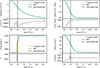 |
Fig. B.1. Comparison of the stellar structures of the initial models of the sim_k and sim_m simulation. Results for the 3-equation model and the MLT model are shown in yellow and green, respectively. We show the temperature, pressure, hydrogen and density profiles from top left to lower right. The difference between the two initial models is shown in the small panels below the profiles. The initial thermal stratifications can be found in Fig. 1. We note that the green and yellow lines largely overlap due to the similarity of the initial stellar models. |
Appendix C: Useful mathematical identities
For the computation of the averages required for the RANS analysis, it is useful to quote a number of identities. Many terms contain averages of at least two fluctuating quantities. These can be conveniently rewritten as
 (C.1)
(C.1)
where we used  . In this way, we avoid computing fluctuations locally to average them subsequently. Instead, we compute averages of the full hydrodynamic variables and reconstruct the correlation functions subsequently. The same procedure may be applied to third-order combinations of fluctuating quantities to obtain

Finally, it is worth noting that taking the average and taking a derivative commute:

(see e.g. Pope 2000, Sect. 3.7). As the averaged quantities only depend on the radius by definition, the second identity has the convenient consequence that applications of the ∇ operator3 reduce to a radial derivative.
Appendix D: Convergence of average values
To understand the robustness of the average values calculated, we analysed how the averages of the different convective variables and the superadiabaticity evolve over the course of the simulation. The results for the sim_k and sim_m simulation are shown in left and right columns of Fig. D.1, respectively. The averaging windows have a length of 1500 h and are offset by 750 h. For the convective variables directly related to the velocity perturbations, that is, the TKE and the convective flux variable, we observe variations that are in agreement with statistical fluctuations as expected for turbulent flows. The same is true for the superadiabaticity and the entropy fluctuations. Towards the TKE boundary, some secular evolution can be observed as the convection is evolving towards a close to adiabatic stratification in the convection zone. This effect is especially pronounced in the sim_k simulation, which had initially a subadiabatic overshooting layer. As the TKE boundary is related to the TKE profile, also the locations of these boundaries do not vary substantially with time. The entropy boundary in the sim_k simulation shows the same behaviour as the superadiabaticity, that is it moves further out with time, as expected. In the sim_m simulation, larger jumps in the location of the entropy boundary can be observed between averaging windows. As we are dealing with an almost flat entropy gradient (i.e. a close to adiabatic stratification) around the entropy boundary, already a small shift in the value of the entropy gradient can shift the location of the boundary by a lot. We can hence conclude that the convective variables have reached a dynamically converged state for the given thermal stratification.
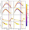 |
Fig. D.1. Analysis of Reynolds averages for the identical length (1500 h) averaging windows, centred at different times. The results of the sim_k and sim_m simulation are given in the left and right panel, respectively. The TKE ω, convective flux variable Π, entropy fluctuation variable Φ and the superadiabaticity are shown from top to bottom. The entropy and TKE boundaries are shown with the dashed and dotted lines, respectively. The colour code correspond to the central time of the averaging windows. |
Appendix E: Convective variables
Figure E.1 shows the TKE of both simulations on a logarithmic scale. For comparison we show the results of the 1D models. On the logarithmic scale it becomes clear that the location of TKE boundary may shift outwards when defining it differently, for example based on the location where a certain fraction of the maximum is reached. For a more detailed discussion of the TKE we refer to Sect. 4.2.
Appendix F: Contributions of individual terms
In this section we show the contributions of the different equation terms to the left-hand side of the equation. We compute the contributions according to Eq. (21). The results for the TKE, the convective flux and the entropy fluctuation equation are shown in Figs. F.1, F.2 and F.3, respectively. The vertical extent of the coloured regions represent the relative importance of each term at each location.
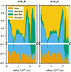 |
Fig. F.1. Radial dependency of the contributions of the absolute values of the terms in Eq. (2). The colours correspond to the individual terms. |
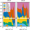
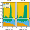
Appendix G: Analysis of individual terms
In this section, we present some additional figures of equation terms that were not shown in the main text.
Appendix G.1: The TKE equation
Figure G.1 shows the buoyancy term of the TKE equation (5). The behaviour of this term is equivalent to the convective flux variable Π discussed in Sect. 4.3. Figure G.2 shows the terms neglected in the TKE equation of the 3-equation model (i.e. Eq. (8)). As discussed before, all terms except for the pressure fluctuation term can be indeed neglected.
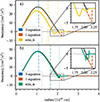 |
Fig. G.1. Comparison of the buoyancy term as a function of radius. The results obtained from the 1- and 3-equation model are shown with a blue and orange line, respectively. The associated RANS correlations extracted from the sim_k and sim_m simulation are shown in the upper panel and lower panel, respectively. We indicate the entropy and TKE boundaries with dashed and dotted lines in the respective colour. The insets show the region of negative convective flux. |
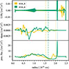 |
Fig. G.2. Comparison of terms neglected in the TKE equation of the Kuhfuß model as a function of radius. The upper panel shows the left hand side of the equation, the middle panels shows the shear term and the lower panel shows the pressure fluctuation terms. The results of the sim_k and sim_m simulation are shown with yellow and green lines, respectively. We indicate the entropy and TKE boundaries with dashed and dotted lines in the respective colour. |
Appendix G.2: Convective flux equation
In Fig. G.3 we show the radiative loss term of the convective flux equation as obtained from the 3D simulations and from the 3-equation model. For visibility reasons we have multiplied the term from the 3-equation model by a factor of 104. Despite this discrepancy between the simulations and the 3-equation model, we find that the radiative loss term is about four orders of magnitude smaller than the other terms in the convective flux equation. Hence, we do not expect a noticeable difference in the results of the 3-equation model if we were to adopt the radiative loss term obtained from the simulations. In Fig. G.4 we show the terms of the convective flux equation that were neglected in the 3-equation model. We again find that the neglecting these term is a justified assumption with the pressure fluctuation term again being the only exception. Finally, Fig. G.5 shows the residuals of the convective flux equation. This can be interpreted as the dissipation of the convective flux in the simulations.
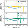
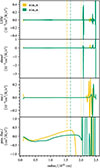 |
Fig. G.4. Comparison of terms neglected in the convective flux equation of the Kuhfuß model as a function of radius. The first panel shows the left hand side of the equation, the second panel shows the shear term, the third panel shows the nuclear energy generation terms and the lower panel shows the pressure fluctuation terms. The results of the sim_k and sim_m simulation are shown with yellow and green lines, respectively. We indicate the entropy and TKE boundaries with dashed and dotted lines in the respective colour. |
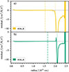 |
Fig. G.5. Comparison of the residuals in the convective flux equation of the Kuhfuß model as a function of radius. The results of the sim_k and sim_m simulation are shown in the upper and lower panel, respectively. We indicate the entropy and TKE boundaries with dashed and dotted lines in the respective colour. |
Appendix G.3: Entropy fluctuation equation
Figure G.6 shows the radiative loss term of the entropy fluctuation equation. This term behaves very similar to the radiative loss term of the convective flux equation. Despite the discrepancy between the 3D simulations and the 3-equation model we do not expect this term to have a big impact on the results of the 3-equation model. In the case of the entropy fluctuation equation all terms that are neglected in the 3-equation model, are indeed found to be negligible in the simulation. Finally, Fig. G.8 shows the residuals of the entropy fluctuation equation.
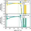
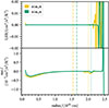 |
Fig. G.7. Comparison of neglected terms in the entropy fluctuation equation of the Kuhfuß model as a function of radius. The upper panel shows the left-hand side of the equation and the lower panel shows the nuclear energy generation terms. The results of the sim_k and sim_m simulation are shown with yellow and green lines, respectively. We indicate the entropy and TKE boundaries with dashed and dotted lines in the respective colour. |
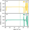 |
Fig. G.8. Comparison of residuals of the entropy fluctuation equation of the Kuhfuß model as a function of radius. The results of the sim_k and sim_m simulation are shown in the upper and lower panel, respectively. We indicate the entropy and TKE boundaries with dashed and dotted lines in the respective colour. |
All Tables
Comparison of the negative convective flux region in the models and simulations.
All Figures
|
Fig. 1. Time-averaged superadiabaticity of the simulations (solid lines) and the initial models (dot-dashed lines). The dot-dashed orange line shows the superadiabaticity of the 1-equation model for comparison. The vertical dashed and dotted lines indicate the position of the entropy and TKE boundary (for definitions, see Sect. 4.1), respectively. |
| In the text | |
|
Fig. 2. Time evolution of the angularly averaged velocity profile. The top and bottom panels show the sim_m simulation and the sim_k simulation, respectively. The end of the initial transient phase is indicated with a vertical dashed white line. |
| In the text | |
|
Fig. 3. Visualisation of the convective flow from the 3D simulations in the x–z and the x–y plane using the Mach number of the flow in the upper and lower panel, respectively. The results from the sim_k simulation are shown in the left column and the results from the sim_m simulation are shown in the right column. The Mach number is indicated with the logarithmic colour-scale. The Schwarzschild boundary of the initial stellar models is indicated with a white dash-dotted line in each panel. We further indicate the entropy and TKE boundary of each simulation with the dashed and dotted white lines (see Sect. 4.1 and Table 1 for details). The upper row shows the raw simulation data, while a radial smoothing has been applied to the flow velocities in the bottom row (see text). The Cartesian coordinates x, y, z are obtained from the conventional conversion of the spherical coordinates r, θ, ϕ of the simulation grid. |
| In the text | |
|
Fig. 4. Comparison of |
| In the text | |
|
Fig. 5. Negative gradient of the mean entropy as a function of radius on a symmetric logarithmic scale. The entropy boundary is indicated with a vertical dashed line in the respective colour. The boundary of the TKE is indicated with a vertical dotted line in the respective colour. The formal Schwarzschild boundary of the initial stellar model computed using MLT is indicated with the dashed dark grey line. |
| In the text | |
|
Fig. 6. Flow isotropy as a function of radius computed from the RANS data obtained from the sim_k and sim_m simulation in yellow and green, respectively. We indicate the entropy and TKE boundaries with dashed and dotted lines in the respective colour. |
| In the text | |
|
Fig. 7. Comparison of the TKE ω as a function of radius. Each panel shows the results obtained from the 1- and 3-equation model and from an MLT model with a blue, orange and black line respectively. The associated RANS correlations extracted from the sim_k and sim_m simulation are shown in the upper panel and lower panel, respectively. We indicate the entropy and TKE boundaries with dashed and dotted lines in the respective colour. |
| In the text | |
|
Fig. 8. Comparison of the convective flux variable Π as a function of radius. The results obtained from the 1- and 3-equation model and from the MLT model are shown with a blue, orange and black line respectively. The associated RANS correlations extracted from the sim_k and sim_m simulation are shown in the upper panel and lower panel, respectively. We indicate the entropy and TKE boundaries with dashed and dotted lines in the respective colour. |
| In the text | |
|
Fig. 9. Comparison of the squared entropy fluctuations Φ as a function of radius. The results from the 3-equation model are shown with a blue line. The associated RANS correlations extracted from the sim_k and sim_m simulation are shown in the upper panel and lower panel, respectively. We indicate the entropy and TKE boundaries with dashed and dotted lines in the respective colour. |
| In the text | |
|
Fig. 10. Comparison of the non-local terms of the TKE equation. The results obtained from the 1- and 3-equation model are shown with a blue and orange line, respectively. The associated RANS correlations extracted from the sim_k and sim_m simulation are shown in the upper panel and lower panel, respectively. We indicate the entropy and TKE boundaries with dashed and dotted lines in the respective colour. |
| In the text | |
|
Fig. 11. Pressure fluctuation term and non-local term of the 3D simulations as a function of radius. The results of the sim_k and sim_m simulation are shown in the upper and lower panel, respectively. The non-local term is scaled with a factor of −2/5 to demonstrate the quality of the closure for the pressure-fluctuation term. We indicate the entropy and TKE boundaries with dashed and dotted lines in the respective colour. |
| In the text | |
|
Fig. 12. Residual term of the 3D simulations as a function of radius. The results of the sim_k and sim_m simulation are shown in the upper and lower panel, respectively. For comparison, we show the dissipation term from the 1- and 3-equation model with an orange and blue line, respectively. We indicate the entropy and TKE boundaries with dashed and dotted lines in the respective colour. |
| In the text | |
|
Fig. 13. Comparison of the non-local term of the convective flux equation Eq. (6) as a function of radius. The results for the sim_k and sim_m simulation are shown in the upper and lower panel, respectively. The results of the 3-equation model are shown with the blue line. We indicate the entropy and TKE boundaries with dashed and dotted lines in the respective colour. |
| In the text | |
|
Fig. 18. Comparison of potential terms of the convective flux equation of the 3-equation model as a function of radius. The results of the sim_k and sim_m simulation are shown with a yellow and green line, respectively. The potential terms of the convective flux equation obtained from the 3-equation model are shown with the remaining coloured lines (see legend for details). The parameters αω, αΠ and αΦ are varied in the upper, middle and lower panel respectively. The mid-blue line indicates the default parameter values. |
| In the text | |
|
Fig. B.1. Comparison of the stellar structures of the initial models of the sim_k and sim_m simulation. Results for the 3-equation model and the MLT model are shown in yellow and green, respectively. We show the temperature, pressure, hydrogen and density profiles from top left to lower right. The difference between the two initial models is shown in the small panels below the profiles. The initial thermal stratifications can be found in Fig. 1. We note that the green and yellow lines largely overlap due to the similarity of the initial stellar models. |
| In the text | |
|
Fig. D.1. Analysis of Reynolds averages for the identical length (1500 h) averaging windows, centred at different times. The results of the sim_k and sim_m simulation are given in the left and right panel, respectively. The TKE ω, convective flux variable Π, entropy fluctuation variable Φ and the superadiabaticity are shown from top to bottom. The entropy and TKE boundaries are shown with the dashed and dotted lines, respectively. The colour code correspond to the central time of the averaging windows. |
| In the text | |
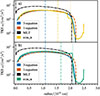 |
Fig. E.1. Same as Fig. 7 on a logarithmic scale. |
| In the text | |
|
Fig. F.1. Radial dependency of the contributions of the absolute values of the terms in Eq. (2). The colours correspond to the individual terms. |
| In the text | |
|
Fig. G.1. Comparison of the buoyancy term as a function of radius. The results obtained from the 1- and 3-equation model are shown with a blue and orange line, respectively. The associated RANS correlations extracted from the sim_k and sim_m simulation are shown in the upper panel and lower panel, respectively. We indicate the entropy and TKE boundaries with dashed and dotted lines in the respective colour. The insets show the region of negative convective flux. |
| In the text | |
|
Fig. G.2. Comparison of terms neglected in the TKE equation of the Kuhfuß model as a function of radius. The upper panel shows the left hand side of the equation, the middle panels shows the shear term and the lower panel shows the pressure fluctuation terms. The results of the sim_k and sim_m simulation are shown with yellow and green lines, respectively. We indicate the entropy and TKE boundaries with dashed and dotted lines in the respective colour. |
| In the text | |
|
Fig. G.4. Comparison of terms neglected in the convective flux equation of the Kuhfuß model as a function of radius. The first panel shows the left hand side of the equation, the second panel shows the shear term, the third panel shows the nuclear energy generation terms and the lower panel shows the pressure fluctuation terms. The results of the sim_k and sim_m simulation are shown with yellow and green lines, respectively. We indicate the entropy and TKE boundaries with dashed and dotted lines in the respective colour. |
| In the text | |
|
Fig. G.5. Comparison of the residuals in the convective flux equation of the Kuhfuß model as a function of radius. The results of the sim_k and sim_m simulation are shown in the upper and lower panel, respectively. We indicate the entropy and TKE boundaries with dashed and dotted lines in the respective colour. |
| In the text | |
|
Fig. G.7. Comparison of neglected terms in the entropy fluctuation equation of the Kuhfuß model as a function of radius. The upper panel shows the left-hand side of the equation and the lower panel shows the nuclear energy generation terms. The results of the sim_k and sim_m simulation are shown with yellow and green lines, respectively. We indicate the entropy and TKE boundaries with dashed and dotted lines in the respective colour. |
| In the text | |
|
Fig. G.8. Comparison of residuals of the entropy fluctuation equation of the Kuhfuß model as a function of radius. The results of the sim_k and sim_m simulation are shown in the upper and lower panel, respectively. We indicate the entropy and TKE boundaries with dashed and dotted lines in the respective colour. |
| In the text | |
Current usage metrics show cumulative count of Article Views (full-text article views including HTML views, PDF and ePub downloads, according to the available data) and Abstracts Views on Vision4Press platform.
Data correspond to usage on the plateform after 2015. The current usage metrics is available 48-96 hours after online publication and is updated daily on week days.
Initial download of the metrics may take a while.