| Issue |
A&A
Volume 705, January 2026
|
|
|---|---|---|
| Article Number | A23 | |
| Number of page(s) | 24 | |
| Section | Extragalactic astronomy | |
| DOI | https://doi.org/10.1051/0004-6361/202555831 | |
| Published online | 08 January 2026 | |
Spatially resolved polarization swings in the supermassive binary black hole candidate OJ 287 with first Event Horizon Telescope observations
1
Instituto de Astrofísica de Andalucía-CSIC, Glorieta de la Astronomía s/n, E-18008 Granada, Spain
2
Korea Astronomy and Space Science Institute, Daedeok-daero 776, Yuseong-gu, Daejeon 34055, Republic of Korea
3
Department of Astronomy, Yonsei University, Yonsei-ro 50, Seodaemun-gu, 03722 Seoul, Republic of Korea
4
Max-Planck-Institut für Radioastronomie, Auf dem Hügel 69, D-53121 Bonn, Germany
5
Massachusetts Institute of Technology Haystack Observatory, 99 Millstone Road, Westford, MA 01886, USA
6
National Astronomical Observatory of Japan, 2-21-1 Osawa, Mitaka, Tokyo 181-8588, Japan
7
Black Hole Initiative at Harvard University, 20 Garden Street, Cambridge, MA 02138, USA
8
Departament d’Astronomia i Astrofísica, Universitat de València, C. Dr. Moliner 50, E-46100 Burjassot, València, Spain
9
Department of Physics, Faculty of Science, Universiti Malaya, 50603 Kuala Lumpur, Malaysia
10
Department of Physics & Astronomy, The University of Texas at San Antonio, One UTSA Circle, San Antonio, TX 78249, USA
11
Physics & Astronomy Department, Rice University, Houston, TX 77005-1827, USA
12
Center for Astrophysics | Harvard & Smithsonian, 60 Garden Street, Cambridge, MA 02138, USA
13
Institute of Astronomy and Astrophysics, Academia Sinica, 11F of Astronomy-Mathematics Building, AS/NTU No. 1, Sec. 4, Roosevelt Rd., Taipei 106216, Taiwan, R.O.C.
14
Observatori Astronòmic, Universitat de València, C. Catedrático José Beltrán 2, E-46980 Paterna, València, Spain
15
Department of Space, Earth and Environment, Chalmers University of Technology, Onsala Space Observatory, SE-43992 Onsala, Sweden
16
Steward Observatory and Department of Astronomy, University of Arizona, 933 N. Cherry Ave., Tucson, AZ 85721, USA
17
Yale Center for Astronomy & Astrophysics, Yale University, 52 Hillhouse Avenue, New Haven, CT 06511, USA
18
Astronomy Department, Universidad de Concepción, Casilla 160-C Concepción, Chile
19
Department of Physics, University of Illinois, 1110 West Green Street, Urbana, IL 61801, USA
20
Fermi National Accelerator Laboratory, MS209, P.O. Box 500 Batavia, IL 60510, USA
21
Department of Astronomy and Astrophysics, University of Chicago, 5640 South Ellis Avenue, Chicago, IL 60637, USA
22
East Asian Observatory, 660 N. A’ohoku Place, Hilo, HI 96720, USA
23
James Clerk Maxwell Telescope (JCMT), 660 N. A’ohoku Place, Hilo, HI 96720, USA
24
California Institute of Technology, 1200 East California Boulevard, Pasadena, CA 91125, USA
25
Institute of Astronomy and Astrophysics, Academia Sinica, Taipei, Taiwan
26
Department of Physics and Astronomy, University of Hawaii at Manoa, 2505 Correa Road, Honolulu, HI 96822, USA
27
Institut de Radioastronomie Millimétrique (IRAM), 300 rue de la Piscine, F-38406 Saint Martin d’Hères, France
28
Perimeter Institute for Theoretical Physics, 31 Caroline Street North, Waterloo, ON N2L 2Y5, Canada
29
Department of Physics and Astronomy, University of Waterloo, 200 University Avenue West, Waterloo, ON N2L 3G1, Canada
30
Waterloo Centre for Astrophysics, University of Waterloo, Waterloo, ON N2L 3G1, Canada
31
Department of Astrophysics, Institute for Mathematics, Astrophysics and Particle Physics (IMAPP), Radboud University, P.O. Box 9010 6500 GL Nijmegen, The Netherlands
32
Department of Astronomy, University of Massachusetts, Amherst, MA 01003, USA
33
Instituto de Astronomia, Geofísica e Ciências Atmosféricas, Universidade de São Paulo, R. do Matão, 1226, São Paulo, SP 05508-090, Brazil
34
Kavli Institute for Cosmological Physics, University of Chicago, 5640 South Ellis Avenue, Chicago, IL 60637, USA
35
Department of Physics, University of Chicago, 5720 South Ellis Avenue, Chicago, IL 60637, USA
36
Enrico Fermi Institute, University of Chicago, 5640 South Ellis Avenue, Chicago, IL 60637, USA
37
Princeton Gravity Initiative, Jadwin Hall, Princeton University, Princeton, NJ 08544, USA
38
Data Science Institute, University of Arizona, 1230 N. Cherry Ave., Tucson, AZ 85721, USA
39
Program in Applied Mathematics, University of Arizona, 617 N. Santa Rita, Tucson, AZ 85721, USA
40
Cornell Center for Astrophysics and Planetary Science, Cornell University, Ithaca, NY 14853, USA
41
Institute of Astronomy and Astrophysics, Academia Sinica, 645 N. A’ohoku Place, Hilo, HI 96720, USA
42
Shanghai Astronomical Observatory, Chinese Academy of Sciences, 80 Nandan Road, Shanghai 200030, People’s Republic of China
43
Key Laboratory of Radio Astronomy and Technology, Chinese Academy of Sciences, A20 Datun Road, Chaoyang District, Beijing 100101, People’s Republic of China
44
WattTime, 490 43rd Street, Unit 221, Oakland, CA 94609, USA
45
Department of Astronomy, University of Illinois at Urbana-Champaign, 1002 West Green Street, Urbana, IL 61801, USA
46
Instituto de Astronomía, Universidad Nacional Autónoma de México (UNAM), Apdo Postal 70-264 Ciudad de México, Mexico
47
Institut für Theoretische Physik, Goethe-Universität Frankfurt, Max-von-Laue-Straße 1, D-60438 Frankfurt am Main, Germany
48
Institute of Astrophysics, Central China Normal University, Wuhan 430079, People’s Republic of China
49
Department of Astrophysical Sciences, Peyton Hall, Princeton University, Princeton, NJ 08544, USA
50
Dipartimento di Fisica “E. Pancini”, Università di Napoli “Federico II”, Compl. Univ. di Monte S. Angelo, Edificio G, Via Cinthia, I-80126 Napoli, Italy
51
INFN Sez. di Napoli, Compl. Univ. di Monte S. Angelo, Edificio G, Via Cinthia, I-80126 Napoli, Italy
52
Wits Centre for Astrophysics, University of the Witwatersrand, 1 Jan Smuts Avenue, Braamfontein, Johannesburg 2050, South Africa
53
Department of Physics, University of Pretoria, Hatfield, Pretoria 0028, South Africa
54
Centre for Radio Astronomy Techniques and Technologies, Department of Physics and Electronics, Rhodes University, Makhanda 6140, South Africa
55
ASTRON, Oude Hoogeveensedijk 4, 7991 PD Dwingeloo, The Netherlands
56
LESIA, Observatoire de Paris, Université PSL, CNRS, Sorbonne Université, Université de Paris, 5 place Jules Janssen, F-92195 Meudon, France
57
JILA and Department of Astrophysical and Planetary Sciences, University of Colorado, Boulder, CO 80309, USA
58
Tsung-Dao Lee Institute, Shanghai Jiao Tong University, Shengrong Road 520, Shanghai 201210, People’s Republic of China
59
National Astronomical Observatories, Chinese Academy of Sciences, 20A Datun Road, Chaoyang District, Beijing 100101, PR China
60
Las Cumbres Observatory, 6740 Cortona Drive, Suite 102, Goleta, CA 93117-5575, USA
61
Department of Physics, University of California, Santa Barbara, CA 93106-9530, USA
62
National Radio Astronomy Observatory, 520 Edgemont Road, Charlottesville, USA
63
Department of Electrical Engineering and Computer Science, Massachusetts Institute of Technology, 32-D476, 77 Massachusetts Ave., Cambridge, MA 02142, USA
64
Google Research, 355 Main St., Cambridge, MA 02142, USA
65
Institut für Theoretische Physik und Astrophysik, Universität Würzburg, Emil-Fischer-Str. 31, Würzburg, Germany
66
Department of History of Science, Harvard University, Cambridge, MA 02138, USA
67
Department of Physics, Harvard University, Cambridge, MA 02138, USA
68
NCSA, University of Illinois, 1205 W. Clark St., Urbana, IL 61801, USA
69
Royal Netherlands Meteorological Institute, Utrechtseweg 297, 3731 GA De Bilt, The Netherlands
70
Dipartimento di Fisica, Università degli Studi di Cagliari, SP Monserrato-Sestu km 0.7, I-09042 Monserrato (CA), Italy
71
INAF – Osservatorio Astronomico di Cagliari, Via della Scienza 5, I-09047 Selargius (CA), Italy
72
INFN, sezione di Cagliari, I-09042 Monserrato (CA), Italy
73
Institute for Mathematics and Interdisciplinary Center for Scientific Computing, Heidelberg University, Im Neuenheimer Feld 205, Heidelberg 69120, Germany
74
Institut für Theoretische Physik, Universität Heidelberg, Philosophenweg 16, 69120 Heidelberg, Germany
75
CP3-Origins, University of Southern Denmark, Campusvej 55, DK-5230 Odense, Denmark
76
Instituto Nacional de Astrofísica, Óptica y Electrónica. Apartado Postal 51 y 216, 72000. Puebla Pue., Mexico
77
Consejo Nacional de Humanidades, Ciencia y Tecnología, Av. Insurgentes Sur 1582, 03940 Ciudad de México, Mexico
78
Key Laboratory for Research in Galaxies and Cosmology, Chinese Academy of Sciences, Shanghai 200030, People’s Republic of China
79
Graduate School of Science, Nagoya City University, Yamanohata 1, Mizuho-cho, Mizuho-ku, Nagoya, 467-8501 Aichi, Japan
80
Mizusawa VLBI Observatory, National Astronomical Observatory of Japan, 2-12 Hoshigaoka, Mizusawa, Oshu, Iwate 023-0861, Japan
81
Department of Physics, McGill University, 3600 rue University, Montréal, QC H3A 2T8, Canada
82
Trottier Space Institute at McGill, 3550 rue University, Montréal, QC H3A 2A7, Canada
83
NOVA Sub-mm Instrumentation Group, Kapteyn Astronomical Institute, University of Groningen, Landleven 12, 9747 AD Groningen, The Netherlands
84
Department of Astronomy, School of Physics, Peking University, Beijing 100871, People’s Republic of China
85
Kavli Institute for Astronomy and Astrophysics, Peking University, Beijing 100871, People’s Republic of China
86
Department of Astronomical Science, The Graduate University for Advanced Studies (SOKENDAI), 2-21-1 Osawa, Mitaka, Tokyo 181-8588, Japan
87
Department of Astronomy, Graduate School of Science, The University of Tokyo, 7-3-1 Hongo, Bunkyo-ku, Tokyo 113-0033, Japan
88
The Institute of Statistical Mathematics, 10-3 Midori-cho, Tachikawa, Tokyo 190-8562, Japan
89
Department of Statistical Science, The Graduate University for Advanced Studies (SOKENDAI), 10-3 Midori-cho, Tachikawa, Tokyo 190-8562, Japan
90
Kavli Institute for the Physics and Mathematics of the Universe, The University of Tokyo, 5-1-5 Kashiwanoha, Kashiwa 277-8583, Japan
91
Leiden Observatory, Leiden University, Postbus 2300 9513 RA Leiden, The Netherlands
92
ASTRAVEO LLC, PO Box 1668 Gloucester, MA 01931, USA
93
Applied Materials Inc., 35 Dory Road, Gloucester, MA 01930, USA
94
Institute for Astrophysical Research, Boston University, 725 Commonwealth Ave., Boston, MA 02215, USA
95
University of Science and Technology, Gajeong-ro 217, Yuseong-gu, Daejeon 34113, Republic of Korea
96
Institute for Cosmic Ray Research, The University of Tokyo, 5-1-5 Kashiwanoha, Kashiwa, Chiba 277-8582, Japan
97
Joint Institute for VLBI ERIC (JIVE), Oude Hoogeveensedijk 4, 7991 PD Dwingeloo, The Netherlands
98
CSIRO, Space and Astronomy, PO Box 76 Epping, NSW 1710, Australia
99
Department of Physics, Ulsan National Institute of Science and Technology (UNIST), Ulsan 44919, Republic of Korea
100
Department of Physics, Korea Advanced Institute of Science and Technology (KAIST), 291 Daehak-ro, Yuseong-gu, Daejeon 34141, Republic of Korea
101
Kogakuin University of Technology & Engineering, Academic Support Center, 2665-1 Nakano, Hachioji, Tokyo 192-0015, Japan
102
Graduate School of Science and Technology, Niigata University, 8050 Ikarashi 2-no-cho, Nishi-ku, Niigata 950-2181, Japan
103
Physics Department, National Sun Yat-Sen University, No. 70, Lien-Hai Road, Kaosiung City 80424, Taiwan, R.O.C.
104
School of Astronomy and Space Science, Nanjing University, Nanjing 210023, People’s Republic of China
105
Key Laboratory of Modern Astronomy and Astrophysics, Nanjing University, Nanjing 210023, People’s Republic of China
106
INAF-Istituto di Radioastronomia, Via P. Gobetti 101, I-40129 Bologna, Italy
107
Common Crawl Foundation, 9663 Santa Monica Blvd. 425, Beverly Hills, CA 90210, USA
108
Instituto de Física, Pontificia Universidad Católica de Valparaíso, Casilla, 4059 Valparaíso, Chile
109
INAF-Istituto di Radioastronomia & Italian ALMA Regional Centre, Via P. Gobetti 101, I-40129 Bologna, Italy
110
Department of Physics, National Taiwan University, No. 1, Sec. 4, Roosevelt Rd., Taipei 106216, Taiwan, R.O.C
111
Instituto de Radioastronomía y Astrofísica, Universidad Nacional Autónoma de México, Morelia 58089, Mexico
112
David Rockefeller Center for Latin American Studies, Harvard University, 1730 Cambridge Street, Cambridge, MA 02138, USA
113
Yunnan Observatories, Chinese Academy of Sciences, Kunming, Yunnan Province, People’s Republic of China
114
Center for Astronomical Mega-Science, Chinese Academy of Sciences, 20A Datun Road, Chaoyang District, Beijing 100012, People’s Republic of China
115
Key Laboratory for the Structure and Evolution of Celestial Objects, Chinese Academy of Sciences, Kunming, People’s Republic of China
116
Anton Pannekoek Institute for Astronomy, University of Amsterdam, Science Park 904, 1098 XH Amsterdam, The Netherlands
117
Gravitation and Astroparticle Physics Amsterdam (GRAPPA) Institute, University of Amsterdam, Science Park 904, 1098 XH Amsterdam, The Netherlands
118
School of Physics and Astronomy, Shanghai Jiao Tong University, Shanghai, China
119
Institut de Radioastronomie Millimétrique (IRAM), Avenida Divina Pastora 7, Local 20, E-18012 Granada, Spain
120
National Institute of Technology, Hachinohe College, 16-1 Uwanotai, Tamonoki, Hachinohe City, Aomori 039-1192, Japan
121
Research Center for Astronomy, Academy of Athens, Soranou Efessiou 4, 115 27 Athens, Greece
122
Department of Physics, Villanova University, 800 Lancaster Avenue, Villanova, PA 19085, USA
123
Physics Department, Washington University, CB 1105, St. Louis, MO 63130, USA
124
Departamento de Matemática da Universidade de Aveiro and Centre for Research and Development in Mathematics and Applications (CIDMA), Campus de Santiago, 3810-193 Aveiro, Portugal
125
School of Physics, Georgia Institute of Technology, 837 State St NW, Atlanta, GA 30332, USA
126
School of Space Research, Kyung Hee University, 1732, Deogyeong-daero, Giheung-gu, Yongin-si, Gyeonggi-do 17104, Republic of Korea
127
Canadian Institute for Theoretical Astrophysics, University of Toronto, 60 St. George Street, Toronto, ON M5S 3H8, Canada
128
Dunlap Institute for Astronomy and Astrophysics, University of Toronto, 50 St. George Street, Toronto, ON M5S 3H4, Canada
129
Canadian Institute for Advanced Research, 180 Dundas St West, Toronto, ON M5G 1Z8, Canada
130
Dipartimento di Fisica, Università di Trieste, I-34127 Trieste, Italy
131
INFN Sez. di Trieste, Trieste, Italy
132
Department of Physics, National Taiwan Normal University, No. 88, Sec. 4, Tingzhou Rd., Taipei 116, Taiwan, R.O.C.
133
Center of Astronomy and Gravitation, National Taiwan Normal University, No. 88, Sec. 4, Tingzhou Road, Taipei 116, Taiwan, R.O.C.
134
Finnish Centre for Astronomy with ESO, University of Turku, FI-20014 Turun Yliopisto, Finland
135
Aalto University Metsähovi Radio Observatory, Metsähovintie 114, FI-02540 Kylmälä, Finland
136
Gemini Observatory/NSF NOIRLab, 670 N. A’ohōkū Place, Hilo, HI 96720, USA
137
Frankfurt Institute for Advanced Studies, Ruth-Moufang-Strasse 1, D-60438 Frankfurt, Germany
138
School of Mathematics, Trinity College, Dublin 2, Ireland
139
Department of Physics, University of Toronto, 60 St. George Street, Toronto, ON M5S 1A7, Canada
140
Department of Physics, Tokyo Institute of Technology, 2-12-1 Ookayama, Meguro-ku, Tokyo 152-8551, Japan
141
Hiroshima Astrophysical Science Center, Hiroshima University, 1-3-1 Kagamiyama, Higashi-Hiroshima, Hiroshima 739-8526, Japan
142
Aalto University Department of Electronics and Nanoengineering, PL 15500, FI-00076 Aalto, Finland
143
Institut de Radioastronomie Millimétrique (IRAM), 300 rue de la Piscine, Saint Martin d’Hères, France
144
Jeremiah Horrocks Institute, University of Central Lancashire, Preston PR1 2HE, UK
145
National Biomedical Imaging Center, Peking University, Beijing 100871, People’s Republic of China
146
College of Future Technology, Peking University, Beijing 100871, People’s Republic of China
147
Tokyo Electron Technology Solutions Limited, 52 Matsunagane, Iwayado, Esashi, Oshu, Iwate 023-1101, Japan
148
Department of Physics and Astronomy, University of Lethbridge, Lethbridge, Alberta T1K 3M4, Canada
149
Netherlands Organisation for Scientific Research (NWO), Postbus 93138 2509 AC Den Haag, The Netherlands
150
Frontier Research Institute for Interdisciplinary Sciences, Tohoku University, Sendai 980-8578, Japan
151
Astronomical Institute, Tohoku University, Sendai 980-8578, Japan
152
Department of Physics and Astronomy, Seoul National University, Gwanak-gu, Seoul 08826, Republic of Korea
153
SNU Astronomy Research Center, Seoul National University, Gwanak-gu, Seoul 08826, Republic of Korea
154
University of New Mexico, Department of Physics and Astronomy, Albuquerque, NM 87131, USA
155
Physics Department, Brandeis University, 415 South Street, Waltham, MA 02453, USA
156
Tuorla Observatory, Department of Physics and Astronomy, University of Turku, FI-20014 Turun Yliopisto, Finland
157
Radboud Excellence Fellow of Radboud University, Nijmegen, The Netherlands
158
School of Natural Sciences, Institute for Advanced Study, 1 Einstein Drive, Princeton, NJ 08540, USA
159
School of Physics, Huazhong University of Science and Technology, Wuhan, Hubei 430074, People’s Republic of China
160
Mullard Space Science Laboratory, University College London, Holmbury St. Mary, Dorking, Surrey RH5 6NT, UK
161
Center for Astronomy and Astrophysics and Department of Physics, Fudan University, Shanghai 200438, People’s Republic of China
162
Astronomy Department, University of Science and Technology of China, Hefei 230026, People’s Republic of China
163
Department of Physics and Astronomy, Michigan State University, 567 Wilson Rd, East Lansing, MI 48824, USA
164
Department of Astronomy and Astrophysics, Tata Institute of Fundamental Research, Mumbai 400005, India
165
Physical Research Laboratory, Mount Abu Observatory, Rajasthan 307501, India
166
INAF – Institute for Space Astrophysics and Planetology, Via Fosso del Cavaliere, 100, 00133 Rome, Italy
★ Corresponding author: This email address is being protected from spambots. You need JavaScript enabled to view it.
Received:
5
June
2025
Accepted:
18
September
2025
Abstract
We present the first Event Horizon Telescope 1.3 mm observations of the supermassive binary black hole candidate OJ 287. The observations achieved an unprecedented angular resolution of 18 μas and reveal significant structural and polarization variability over just five days, marking the shortest timescale on which such changes have been directly imaged in this source. The inner jet exhibits a twisted ridgeline structure, with features displaying apparent superluminal motions up to about 22 c. The linear polarization maps reveal three main polarized features whose electric-vector position angles (EVPAs) change substantially over the time span of our observations, including a component with a radial polarization consistent with being produced by a recollimation shock. Most notably, we directly resolved two innermost jet components whose EVPAs rotate in opposite directions. The faster component, moving at 2.4 ± 0.9 μas/day (17.4 ± 6.5 c), exhibits counterclockwise EVPA swings of roughly 3.7° per day, while the slower component, with a proper motion of 1.4 ± 0.3 μas/day (10.2 ± 2.2 c), rotates clockwise at approximately 2.5° per day. Previous studies inferred helical magnetic fields in AGN jets from time-resolved or integrated polarization variability but lacked the angular resolution to directly image this effect. Our results provide spatially resolved evidence that a helical magnetic field threads the jet’s collimation and acceleration zone, ruling out models based on the superposition of unresolved components. Our analysis suggests that propagating shocks interact with a Kelvin–Helmholtz plasma instability, illuminating different phases of the helical magnetic field and producing the observed polarization spatial and temporal variability. Moreover, our model naturally accounts for the more rapid polarization rotation observed in the faster moving component. Our model predicts even more rapid swings in polarization, which could be tested with future observations featuring a more densely sampled time coverage.
Key words: black hole physics / instabilities / radiation mechanisms: non-thermal / techniques: interferometric / galaxies: active / galaxies: individual: OJ 287
NASAHubble Fellowship Program, Einstein Fellow.
Deceased.
© The Authors 2026
 Open Access article, published by EDP Sciences, under the terms of the Creative Commons Attribution License (https://creativecommons.org/licenses/by/4.0), which permits unrestricted use, distribution, and reproduction in any medium, provided the original work is properly cited.
This article is published in open access under the Subscribe to Open model. This email address is being protected from spambots. You need JavaScript enabled to view it. to support open access publication.
1. Introduction
The BL Lacertae object OJ 287 is an emblematic nearby active galactic nucleus (AGN) with a redshift of z = 0.306 (Stickel et al. 1989), well known for its 12-year quasi-periodic outbursts in the optical regime (e.g., Sillanpää et al. 1988; Villata et al. 1998). These quasi-periodic variations have been interpreted as evidence of a supermassive black hole binary (SMBHB) system where the secondary black hole, in a highly eccentric orbit around the central black hole, modulates the jet emission as it interacts with the primary’s accretion disk. This model was used to explain the quasi-periodic variability (Lehto & Valtonen 1996; Valtaoja et al. 2000; Valtonen et al. 2008), which aligns with theoretical models of an accreting SMBHB based on general relativistic magnetohydrodynamics simulations, which account for dynamic spacetime effects in accreting binary systems (Farris et al. 2012; Gold et al. 2014a,b; Gold 2019; Paschalidis et al. 2021). Supporting the binary scenario, Britzen et al. (2018) identified a 23-year jet precession period that was later corroborated by Britzen et al. (2023), who linked spectral energy distribution (SED) states to the precession phase. On the other hand, the presence of an ultra-massive primary black hole has been put into question by multi-frequency observations and a lack of predicted outbursts (Komossa et al. 2023a,b) in the years 2021 and 2022. The authors raising these doubts showed that the data favor more periodic outbursts with a period of 11.5 ± 1 yr, most recently observed in 2016–2017, and they estimated the mass of the primary to be 108 M⊙.
Variations in the jet position angle can also be explained by alternative scenarios that do not require a SMBHB system. For instance, the precession of a single misaligned accretion disk around a single central supermassive black hole (SMBH) (Mizuno et al. 2012), or a warped accretion disk, not perfectly aligned with the black hole spin axis (Liska et al. 2018). Beyond these mechanisms, several internal processes can generate similar observational signatures in AGN jets. For example, jet instabilities play a fundamental role in AGN jet phenomenology.
Two types of instabilities are mainly encountered in AGN jets: Kelvin-Helmholtz (K-H) instabilities and current-driven instabilities (CDI). The K-H instabilities, which arise from velocity shear between the jet and the ambient medium, can develop in kinetically dominated jets (e.g., Perucho et al. 2004; Hardee 2007). These instabilities can generate helical perturbations that manifest as twisted structures when projected onto the plane of the sky (Perucho et al. 2012; Vega-García et al. 2019). Additionally, CDI kink instabilities can develop in strongly magnetized jets (e.g., Nakamura et al. 2007; Mizuno et al. 2012), further contributing to jet wiggling and bending. These various instability modes, coupled with recollimation shocks and magnetic field compression, can drive internal shocks and turbulence, potentially explaining the observed variability in AGNs (Marscher 2014; Jorstad et al. 2022) and playing a crucial role in particle acceleration mechanisms (Sironi et al. 2015). In fact, OJ 287 constitutes an ideal laboratory for investigating particle acceleration mechanisms, as it has an emission spectrum stretched up to teraelectron-volt energies (e.g., Mukherjee & VERITAS Collaboration 2017; Lico et al. 2022). It also provides a critical platform of testing the validity of different launching scenarios of AGN jets, as theoretical models suggest that relativistic jets are produced by accreting SMBH and driven by their dynamically important magnetic fields, which can be twisted by the ergosphere (Blandford & Znajek 1977) or by the differential rotation of the black hole’s accretion disk (Blandford & Payne 1982).
Very long baseline interferometry (VLBI) observations at the highest possible angular resolution are the ideal method for probing the innermost regions of AGN jets. This can be achieved by either increasing the observing frequency or extending the baselines to include space-based antennas. Indeed, with an apogee of approximately 350 000 km, space VLBI observations with RadioAstron have been capable of imaging blazar jets with unprecedented resolution, on the order of a few tens of microarcseconds (e.g., Gómez et al. 2016; Fuentes et al. 2023). During its operation, RadioAstron observed OJ 287 on several epochs, yielding the highest angular resolution image obtained for this source (Gómez et al. 2022). Most recently, space-based VLBI imaging of OJ 287 with RadioAstron at 22 GHz, together with multi-epoch Very Long Baseline Array (VLBA) observations at 43 GHz, revealed a ribbon-like inner-jet morphology and multi-year swings of the jet position angle that are consistent with a rotating helical jet structure on parsec scales (Traianou et al. 2025).
Event Horizon Telescope (EHT) observations at 1.3 mm have also significantly advanced our understanding of SMBHs and their relativistic jets, culminating in the groundbreaking capture of the first images of a black hole in M87 (Event Horizon Telescope Collaboration 2019a,b,c,d,e,f, 2021a,b, 2023), hereafter M87* Papers I–IX) and Sgr A∗ (Event Horizon Telescope Collaboration 2022a,b,c,d,e,f, 2024a,b, hereafter Sgr A∗ Papers I–VIII) and demonstrating that black holes with masses ranging from millions to billions of solar masses can be consistently described by the Kerr metric. Building on this foundational work, EHT observations of a number of AGNs have provided a crucial window into the physics of jet launching and initial collimation in extragalactic radio jets at scales down to 10–100 gravitational radii, encompassing the processes of jet launch and its initial collimation (e.g., Kim et al. 2020; Janssen et al. 2021; Issaoun et al. 2022; Jorstad et al. 2023; Paraschos et al. 2024; Baczko et al. 2024; Röder et al. 2025).
In April 2017, we conducted the inaugural 1.3 mm VLBI observations of OJ 287 with the EHT in order to probe its structure at scales corresponding to the hypothesized presence of a SMBHB system. These observations were part of an extensive multiwavelength campaign including additional longer wavelength VLBI observations from both ground- and space-based facilities such as RadioAstron (Gómez et al. 2022) and the Global Millimeter VLBI Array (GMVA; Zhao et al. 2022) and alongside observations in optical, UV, and X-ray wavebands (e.g., Komossa et al. 2021a; EHT MWL Science Working Group et al. 2021, on OJ 287 and M 87, respectively). Concurrently, the independent Multiwavelength Observations and Modelling of OJ 287 (MOMO) project, which started in 2015, has provided a framework for these integrated studies (e.g. Komossa et al. 2017, 2021b, 2023a). MOMO provides high-cadence optical, UV, X-ray, and MWL single-dish radio observations and their interpretation. OJ 287 has also been regularly monitored with the VLBA at 43 GHz and 15 GHz for over two decades as part of the BEAM-ME1 (Jorstad & Marscher 2016; Jorstad et al. 2017; Weaver et al. 2022) and MOJAVE2 (Lister et al. 2018) monitoring programs, respectively.
This work is organized as follows: In Section 2, we describe the EHT observations, data reduction, and imaging techniques used to reconstruct the total intensity and polarization structure of the source. Section 3 presents the results, detailing the detected variability in total intensity and polarization over a five-day timescale, the characterization of jet features, and the measured apparent motions. In Section 4, we discuss the implications of these findings in the context of relativistic jet physics, focusing on the role of K-H instabilities, shocks, and a helical magnetic field in explaining the observed variability. We introduce a model that accounts for the rapid polarization swings and outline how future observations with improved time sampling could further test these predictions. In Section 5, we provide a summary of our results. We note that for all the calculations, we adopt a flat ΛCDM cosmology with H0 = 67.4 km s−1 Mpc−1, Ωm = 0.315, and ΩΛ = 0.685 (Planck Collaboration VI 2020). At the redshift of OJ 287, this corresponds to a luminosity distance of 1.642 Gpc, an angular scale of 4.65 pc mas−1, and an apparent speed of 7.25 c for a proper motion of 1 μas day−1.
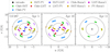 |
Fig. 1. Event Horizon Telescope (u, v)-coverage of the OJ 287 observations on April 5, 10, and 11, 2017. Each colored point corresponds to a single VLBI scan of ∼5 min. Dashed line circles indicate the fringe spacing of 50 μas and 25 μas. “Chile” represents the stations ALMA and APEX. “Hawai’i” represents the stations SMA and JCMT. |
2. Observations and data analysis
2.1. Observations and calibration
The EHT observed OJ 287 on three nights during the 2017 campaign on April 5, 10, and 11. Two of those days, April 5 and 10, offer sufficient (u, v) coverage to fully model the source structure in total intensity and in linear polarization. Additionally, the coverage is similar enough to reliably compare results between days (see Figure 1). The source was observed with the array consisting of seven telescopes located at five geographic sites: the Atacama Large Millimeter/submillimeter Array (ALMA, operating as a phased array; Goddi et al. 2019) and the Atacama Pathfinder Experiment (APEX) telescope in Chile; the Large Millimeter Telescope Alfonso Serrano (LMT) in Mexico; the IRAM 30 m telescope (PV) in Spain; the Submillimeter Telescope (SMT) in Arizona; and the James Clerk Maxwell Telescope (JCMT) and the Submillimeter Array (SMA) in Hawai’i. The source is not visible from the South Pole Telescope (SPT), which also participated in the EHT campaign. The observations were carried out with two 2 GHz-wide frequency bands centered at 227.1 GHz (LO band) and 229.1 GHz (HI band). Right-hand circularly polarized and left-hand circularly polarized signals were recorded for all stations other than ALMA and JCMT. ALMA recorded dual linear polarization, which was subsequently converted at the correlation stage to a circular basis using PolConvert (Martí-Vidal et al. 2016; Goddi et al. 2019). JCMT observed a single circular polarization component, which we used to approximate the total intensity under the assumption that the circular polarization can be neglected, and moreover the JCMT baselines were flagged for the polarimetric imaging. The configuration of the EHT array during the 2017 campaign is described in detail in M87PaperII.
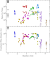 |
Fig. 2. Signal-to-noise ratio of OJ 287 detections on April 10, 2017 (top panel), and the corresponding visibility amplitudes of the calibrated data set (bottom panel). Both frequency bands are shown, with scan-long (typically ∼5 min) averaging. Colors follow the convention of Fig. 1. Circle markers denote baselines with ALMA or SMA, while diamonds denote similar baselines to APEX or JCMT. |
Recorded signals were correlated at the MIT Haystack Observatory in Westford (MA, USA) and the Max-Planck-Institut für Radioastronomie in Bonn (Germany) (Deller et al. 2011; M87PaperII). Subsequent data reduction procedures were described in M87PaperIII; Blackburn et al. (2019), Janssen et al. (2019). There were minor updates to the calibration pipeline with respect to the EHT results published earlier (M87PaperI; Kim et al. 2020), particularly regarding the telescopes sensitivity estimates and complex polarimetric gains calibration. These updates are identical with the ones employed for the EHT Sgr A∗ publications (SgraP1; SgraP2). Flux density on the short intra-site baselines (ALMA-APEX and SMA-JCMT) was gain-calibrated to the simultaneous ALMA-only flux densities reported by Goddi et al. (2021), that is 4.34 Jy on April 5 and 4.22 Jy on April 10. The polarimetric leakage calibration follows procedures outlined in M87PaperVII, with the fiducial D-terms given by M87PaperVII and Issaoun et al. (2022), also verified by Jorstad et al. (2023). Wide observing frequency bands and effective calibration resulted in high signal-to-noise (S/N) ratio detections, reaching ∼1000 on ALMA baselines for data coherently averaged over observing scans, lasting ∼5 minutes (see Figure 2).
2.2. Imaging
Image reconstruction of OJ 287 has been performed in a similar manner to previous EHT results. The images presented in this paper were obtained with three different algorithms: CLEAN, implemented in the software library DIFMAP (Shepherd 1997); regularized maximum likelihood (RML), implemented in the eht-imaging (Chael et al. 2016, 2018), SMILI (Akiyama et al. 2017a,b) and DoG-HiT (Müller & Lobanov 2022) packages; and Bayesian posterior exploration methods, implemented in the modeling frameworks DMC and THEMIS. (Broderick et al. 2020a; Pesce 2021). See Janssen et al. (2022) for an overview of the presently available software for advanced VLBI anlaysis.
The traditionally used algorithm for imaging interferometric data at radio wavelengths, CLEAN, has proved its ability to successfully reconstruct the 1.3 mm emission surrounding the SMBH in M 87, Sgr A∗, and several AGN sources. Based on the assumption that the sky brightness distribution of the observed source can be well described by a set of point sources, CLEAN deconvolves the interferometer point source response (i.e., “dirty beam”) from the so-called dirty-image, i.e., the inverse Fourier transform of the measured visibilities. This task is carried out in a iterative process of “cleaning” and self-calibration. To prevent the dominant influence of the phased-ALMA baselines, which possess a significantly higher S/N, the phase and amplitude self-calibration process employed a down-weighting strategy (correction factor 0.1) on all baselines to phased ALMA, ensuring a more balanced calibration procedure.
In contrast, RML methods do not involve the inverse Fourier transform of the visibilities, V, in the imaging process. Instead, they find an image, I, that best minimizes the objective function:
 (1)
(1)
In this equation, the data likelihood and image regularization terms compete for the image solution, modulated by the relative weighting of the hyperparameters αD and βR. Several data products, D, and image-domain regularizers, R, can be incorporated into the optimization process simultaneously. In particular, RML methods can naturally use closure phases and (log) closure amplitudes in addition to complex visibilities, which allow the algorithms to mitigate the effect of phase- and antenna-based errors in the data (e.g., Chael et al. 2018). For each of these data products, the data likelihood takes the form of a reduced χ2, as described in M87PaperIV. The regularization cost functions, SR, include maximum entropy, total variation, and sparsity priors.
DoG-HiT (Müller & Lobanov 2022) approaches the imaging problem in the framework of RML methods and compressed sensing as well. The image is modeled by a dictionary of difference of Gaussian wavelets. These wavelets define radial filters in the u, v-domain and are fit to the u, v-coverage to allow for a better separation between covered baselines and gaps in the u, v-coverage. DoG-HiT performs amplitude conserving imaging by using closure quantities as data fidelity term and the sparsity promoting l0 norm. of the wavelet coefficients as regularization term. Minimization is done by a proximal-point based forward-backward algorithm.
DMC (Pesce 2021) and THEMIS (Broderick et al. 2020a,b) formulate the imaging problem as one of Bayesian posterior exploration, in which the image structure and station-based calibration quantities are simultaneously modeled. Both DMC and THEMIS fit to complex visibilities, for which the likelihood function is Gaussian, and both codes solve for time-dependent complex station-based gains and time-independent complex station-based leakage terms alongside a pixel-based parameterization of the polarized image structure. The output of each code is a set of MCMC samples from the joint posterior distribution over both the full-Stokes image structure and the calibration quantities.
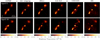 |
Fig. 3. Total intensity images of OJ 287 on April 5 and 10 for different imaging pipelines. The RML imaging methods are separated by a dashed black line, while the Bayesian imaging methods are separated by a solid black line. The DIFMAP images are convolved with a circular Gaussian of 18 μas, corresponding to the maximum of the minor axes of the CLEAN beams (which are approximately circular) of April 5 and 10. For each day, the image resolution of all images are matched with the DIFMAP image resolution as described in Appendix A. |
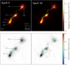 |
Fig. 4. Mean total intensity (top) and linear polarization (bottom) images of OJ 287 on April 5 (left) and 10 (right). Total intensity image is averaged across six different imaging methods for each day using the images from Figure 3. The color scale is the same for both days in units of brightness temperature, as shown at the right color bar. Model-fit components (see Sect. 3.1 and Table 1) are labeled in the April 5 image. Ridgelines (see Sect. 3.1 are shown for both epochs (April 5 and 10 with green and white, respectively). The effective resolution, 18 μas, is shown at the bottom, left corner of the first panel. The linear polarization image is averaged across three imaging methods of DIFMAP, DMC, and eht-imaging (see Appendix B and Figure B.2). The grayscale image shows the total intensity for comparison, while white contours represent polarization intensity at 20, 40, 60, and 80% of the peak value. Ticks indicate linear polarization, with their length corresponding to flux density, angle representing EVPAs, and color denoting fractional polarization, as shown in the color bar on the right. The fit components in polarization (see Sect. 3.2 and Table 2) are labeled in the April 5 image. Components P1, P2, and P3* correspond to the model-fit components C1, C2, and the complex region that includes C3a and C3b, respectively. |
Model-fitting results of OJ 287.
Linear polarization properties of model components showing interday variability.
3. Results
3.1. Total intensity images and model fitting
The total intensity images of OJ 287 from April 5 and 10 are presented in Figure 3, reconstructed using various imaging algorithms. These images showcase the structure of the innermost 200 μas of the jet with an unprecedented angular resolution of 18 μas. DoG-HiT imaging tends to show more compact components, while DMC is more prone to producing more diffuse emission. Similar to previous results at lower frequencies (e.g., Gómez et al. 2022; Zhao et al. 2022), the jet extends in a northwest direction, but the EHT observations at 230 GHz provide a more detailed view, revealing multiple distinct components. The consistency of these structures across six independent reconstructions confirms their robustness, demonstrating that they are not biased by any specific imaging algorithm or parameter settings (Figure 3). Based on their consistency, all the images have been averaged (Figure 4), and subsequent discussions are based on this composite image. It is important to note that, for the averaging process, the center of each image was aligned through normalized cross-correlation, and the different effective resolutions were harmonized (see Appendix A)
We parameterized the flux density distribution along the OJ 287 jet by fitting circular Gaussian model components to the complex visibilities. This was done using the Levenberg-Marquardt algorithm for non-linear least squares minimization in DIFMAP. Prior to fitting, the complex visibilities were self-calibrated for both phases and amplitudes using the averaged image (Figure 4). This analysis successfully described the self-calibrated visibility data with six Gaussian components, achieving an S/N in the residual image (i.e., the ratio of peak to root-mean-squared flux density) of less than five. Although more complex models with additional components were considered, they only added complexity without significantly improving the fit quality. The uncertainties of the model fitting parameters were estimated following the method described by Schinzel et al. (2012). The results of the model fitting are summarized in Table 1 (see also Section 3.3 and Figure 8 for a more visual representation).
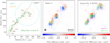 |
Fig. 8. (Left) Fit circular Gaussian model components (full-width half maximum) for April 5 (cyan) and 10 (orange). The relative position of the components are referenced to the innermost component, C0a. The red arrow shows the motion of each component from April 5 to 10, and the solid green line shows the ridgeline of April 10. The broken black line indicates the jet direction obtained by connecting the components’ positions of C0a, C2, and C3a of April 5. (Middle) The Stokes I image difference between epochs (i.e., Iij(Apr. 10) − Iij(Apr. 5), where Iij is the intensity at a pixel (i, j)). The color scale is shown at the bottom of the panel. Note that the flux changes are consistent with the motion of components. (Right) Same as the middle panel but for the linear polarization. The EVPAs at each epoch are shown together (purple and green for April 5 and 10, respectively). The contours in the middle and right panels show the Stokes I structure on April 5 (cyan) and 10 (orange), which are set to 25, 50, 75% of the peak intensity. |
The brightness temperatures for the model fitting components were computed via the relation (e.g., Pushkarev & Kovalev 2012)
 (2)
(2)
where S is the component flux density in Jy, θobs is the size of the emitting region in mas, ν is the observing frequency in GHz, and z is the source redshift. The estimated brightness temperatures in the source frame are listed in Table 1.
In Figure 4, the jet structure consistently extends from southeast to northwest across both observing epochs. The bright emission at the southeastern end of the jet is identified as the VLBI core at 230 GHz, characterized by its compact size, non-polarized nature, and flat spectral profile (see Sect. 4.2). Model fitting in this core area has revealed two distinct components, C0a and C0b. Positions of all components are referenced to C0a, the upstream component, which is assumed to remain stationary over time. Downstream of the core area, the jet bends slightly northward, corresponding to component C1. Further downstream, the jet extends along a position angle roughly estimated at −37° (east of north). This portion of the jet exhibits two prominent features, one labeled C2 and another consisting of two sub-components, C3a and C3b, which we refer to as the C3* complex. Faint jet emission is observed connecting the core with these bright components. To better characterize this, we have employed the filament fitting method described in Fuentes et al. (2023) to determine the jet ridgeline, corresponding to the path traced by the peak brightness along the jet emission. The fitting for both observing epochs reveals a bent structure that resembles a helix in projection, indicating also some structural changes between the two observing epochs (see Sect. 3.3).
3.2. Linear polarization
The bottom part of Figure 4 shows the linear polarization images of OJ 287 from the observations on April 5 and 10, 2017. The images reveal a polarized jet structure dominated by three main features, which are evident in both epochs. These polarization maps highlight the electric vector position angles (EVPAs) overlaid on the total intensity images, providing insights into the underlying magnetic field structure of the jet.
To obtain the polarization images, it is essential to first correct for the instrumental polarization, also known as D-terms. These were corrected using the values derived from the M87∗ observations M87PaperVII. Following this calibration, the polarization images were created by averaging the results from three different methods: CLEAN (DIFMAP), regularized maximum likelihood (eht-imaging), and Bayesian posterior exploration (DMC). This approach was applied consistently to both the polarization and total intensity (Stokes I) images (see also Sect. 3.1), ensuring a uniform treatment across all Stokes parameters (see Appendix B for details on the images from individual pipelines).
The polarization images reveal an unpolarized core region, corresponding to components C0a and C0b. While this could in part be due to the higher opacity observed in the core (see Sect. 4.2), a more likely explanation is beam depolarization from an unresolved helical magnetic field viewed at a small angle (see also Sect. 4.4).
The polarized emission shown in Fig. 4 is dominated by three distinct components: P1, P2, and P3*. These components roughly correspond to C1, C2, and C3* (i.e., C3a + C3b) in the total intensity images. Notably, we observe significant changes in the polarization across these components over the short five-day timescale between the two observing epochs, highlighting the dynamic nature of the jet’s magnetic field structure mapped by these components (see Sect. 3.3).
In Table 2, we list the polarization parameters for the three dominant components, P1, P2, and P3*. These values were computed by averaging the polarization properties over the spatial area corresponding to each component in the images, without weighting the averages by the local polarized intensity. For each component, we also quote an EVPA “error”, defined as the intra-component EVPA dispersion, that is, the standard deviation of pixel-by-pixel EVPAs within the fit component area. This quantity measures EVPA non-uniformity inside the component and is not a systematic or thermal error, which we estimate to be approximately one degree. While this method provides a good representation for P1 and P2, it does not fully capture the complex internal structure of P3*, where significant variations in polarization are present.
Figure 5 shows the details of the C3*/P3* component. On April 5, the EVPAs present a clear radial distribution, while on April 10, the EVPAs follow a curled distribution. We analyze these different patterns by plotting the linear polarization intensity P, the degree of polarization m, and the EVPAs along concentric circular sections centered in the C3*/P3* component (see Figure 6). Both P and m show peaks in the northern direction, which remain consistent across both epochs. However, the EVPA shifts from an almost purely radial field to one where both toroidal and radial components are present. The degree of linear polarization is relatively high across all components. The more homogeneous components, P1 and P2, show mean polarization values of around 20% in both epochs (see Table 2). In contrast, P3* exhibits more variability, with peak polarization values in the northern direction reaching approximately 25%, despite a lower average degree of polarization when integrated over the entire component due to its complex internal EVPA structure. These high polarization values suggest a well-ordered magnetic field structure.
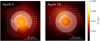 |
Fig. 5. Detail of the C3*/P3* component. The color map represents the total intensity image, while the white ticks represent the polarization vector. The length of the ticks represents the polarization intensity P, while their orientation is that of the EVPA. To analyze the clearly radial/circular pattern of the polarization vector field, we evaluate P, m, and the EVPA along circular sections of the image (see Fig. 6). The shaded area marks the ranges of angles and radii taken into consideration and the circular arrow indicates the convention for the direction and orientation of the angular coordinate ϕ. |
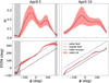 |
Fig. 6. Fractional polarization, m, and EVPA of the C3*/P3* component, evaluated along concentric circular sections (see Fig. 5). The dark red line marks the average values across all range of radii considered, while the red shaded area represents the corresponding standard deviation. The black dotted line shows the EVPA of a purely radial polarization field, while the black dashed line shows the EVPA of a purely tangent polarization field. The gray shaded areas indicate the angles excluded from consideration because they coincide with regions below the noise threshold. |
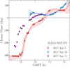 |
Fig. 7. Closure phases measured on a wide triangle between ALMA, SMT, and Pico Veleta. The data shown correspond to the LO band, averaged coherently in 300 s segments before calculating closure products. Continuous lines represent the closure phase values predicted by models obtained by averaging the results from six different imaging algorithms for April 5 and 10, 2017, as shown in Sect. 2.2. The range of modeling predictions for each observing day is shaded. Interday variation of closure phase values indicates the time evolution of the source morphology. |
The very peculiar EVPAs observed in P3* resemble those seen in previous 3 mm VLBI observations of OJ 287 with the GMVA + ALMA (Zhao et al. 2022), indicating a highly structured magnetic field. These EVPAs, combined with the high degree of polarization in P3*, suggest the presence of a recollimation shock, which can compress the magnetic field and produce enhanced polarization and distinct EVPA patterns (e.g., Gómez et al. 1997, 2016; Cawthorne et al. 2013; Mizuno et al. 2015). Notably, at lower frequencies, the jet is observed to bend eastward at P3*/C3* (e.g., Cohen et al. 2018; Gómez et al. 2022), further supporting the presence of a recollimation shock as the jet plasma interacts with the surrounding medium and undergoes changes in pressure.
The source integrated degree of polarization for both days is ∼10% (see Table 2), which is in agreement with the ALMA array results of 7 − 9% presented in Goddi et al. (2021), considering the estimated uncertainties.
3.3. Interday variability
Closure phases encode the structure of the source, making it possible to study potential structural changes across our two observing epochs by examining how the closure phases evolve over time. Figure 7 presents the closure phases measured on a triangle formed by the ALMA, SMT, and Pico Veleta stations, comparing observations from April 5 and 10, 2017. The closure phase data, averaged over 300-second intervals, show clear differences between the two observing dates, providing strong evidence of structural changes in the source over this short timescale, even before the imaging process.
These changes are confirmed through imaging, as seen in Figure 4, where both total intensity and linear polarization reveal clear differences in the source structure between the two observing epochs. The changes are further analyzed in Figure 8, which provides a more detailed comparison of the source’s total intensity and polarization structure across the two dates. This figure highlights the evolving features in both the brightness distribution and the EVPAs, confirming significant structural and magnetic field changes over the five-day interval, which represents the shortest timescale on which such variability has been imaged in OJ 287. Similarly rapid structural changes were also observed in EHT observations of 3C 279 (Kim et al. 2020).
The proper motions of the jet components, listed in Table 1, show a wide range of apparent velocities. In the innermost part of the jet, component C0b exhibits a relatively slow apparent velocity of 2.2 ± 2.2 c, while further downstream, components move significantly faster, with C1 reaching speeds of 17.4 ± 6.5 c. Components C3a and C3b also show very large proper motions, at 22.5 ± 5.1 c and 16.7 ± 9.4 c, respectively. However, these rapid motions may not reflect actual fluid or pattern velocity but could instead be associated with internal changes in the brightness distribution within the C3a + C3b complex, previously associated with a recollimation shock (e.g., Hodgson et al. 2017; Zhao et al. 2022). These values are in agreement with previous estimates from the Boston University monitoring program3, which reports superluminal velocities for OJ 287 jet components reaching up to 19 c (Weaver et al. 2022).
Additionally, the flux density changes between C0a and C0b suggest a possible new injection of plasma into the jet. The increase in flux density in C0b, coupled with a decrease in C0a, indicates a flux transfer between the two components, consistent with new material being injected into the jet that is redistributed as the system evolved over the two days. This flux transfer is also visible in the middle panel of Figure 8, where emission appears to be moving downstream in the inner part of the jet, further supporting this scenario.
The left panel of Figure 8 presents the fit jet ridgeline for April 10, along with the model-fit components for both observing epochs. The ridgeline exhibits a twisted structure, which is evident in both the April 5 and April 10 observations (see also Figure 4). By comparing the proper motions of the components, indicated by arrows, with the local jet direction, we find that their trajectories are neither ballistic, as one might expect from direct ejections from the core, nor do they follow the curvature of the jet ridgeline. This deviation points to more complex dynamics governing the motion of the components within the jet.
In addition to the flux transfer between C0a and C0b, the middle panel of Figure 8 highlights flux density changes in the regions corresponding to C2 and the C3a + C3b complex, consistent with the proper motions of the model-fit components. These variations align with the high apparent velocities described earlier, further confirming the dynamic evolution of the jet structure.
The right panel of Figure 8 highlights the changes in polarization across the two epochs, showing that the variations in linear polarization are consistent with those observed in total intensity. The components exhibit proper motions at an angle to the jet ridgeline, and the EVPAs also align at an angle relative to the ridgeline. Notably, a significant change in the EVPAs is observed between April 5 and April 10, underscoring the dynamic nature of the polarization structure.
The polarization values listed in Table 2 support this variability. Both P1 and P2 maintain relatively stable polarization levels, with their degrees of polarization increasing slightly between the two epochs. However, the EVPAs for these components shift considerably, with P1 rotating by approximately 18° and P2 by about −12°, indicating changes in the orientation of the magnetic field in the regions probed by the components along their motion. As discussed in Sect. 3.2, the polarization structure of C3*/P3* exhibits a complex EVPA pattern, transitioning from an almost purely radial distribution to one that includes both toroidal and radial components.
4. Discussion
In this section, we integrate our findings to construct a detailed understanding of the physical mechanisms underlying the observed variability in OJ 287. We begin by analyzing the optical polarization, which provides critical insights into the magnetic field configuration within the jet. Subsequently, we discuss the nature of the standing feature P3*, its role as a potential recollimation shock, and its implications for downstream jet dynamics. We proceed by examining the spectral index and the position of the core to elucidate the conditions prevailing at the jet base. The link between jet structure and high-energy emission, particularly γ-ray and X-ray activity, is then explored. Additionally, we consider the orientation and evolution of the jet in the context of the binary black hole model, providing a broader astrophysical framework for the system. Lastly, we present a cohesive model that explains the observed interday variability as resulting from K-H instabilities and propagating shocks in a jet threaded by a helical magnetic field.
4.1. Optical polarization and its relationship to the jet features
OJ 287 has been regularly monitored at optical wavelengths by the Boston University blazar group4 with the 1.8 m Perkins telescope (Flagstaff, AZ, USA), and by the St. Petersburg University group with the 0.7 m AZT-8 telescope (CrAO, Crimea). These observations include both photometric and polarimetric measurements in R-band (λeff = 635 nm). A more detailed description of the observations and data reduction can be found in Jorstad et al. (2010).
Figure 9 shows the R-band light curve, degree of polarization, and position angle of polarization of OJ 287 within about a month period around the EHT 2017 campaign. We can see that OJ 287 steadily decreased in optical brightness (as previously reported in the optical band with Swift; Komossa et al. 2021b) from ∼8 mJy down to 4 mJy over ∼25 days. Taking the latter as the timescale of variability (τ) of the optical emission, we can estimate the maximum angular size of the optical emission region as a ≲ cτ(1 + z)δ/DL (Jorstad et al. 2005), where c is the speed of light, DL is the luminosity distance, and δ is the Doppler factor. We adopt δ ∼ 15 based on VLBA monitoring at 43 GHz of superluminal knots near the epoch of the EHT campaign, as found by Weaver et al. (2022). These values yield a compact size of a ≲ 53 μas.
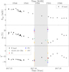 |
Fig. 9. Measurements of the optical light curve, polarization degree, and position angle of OJ 287 by the 1.8 m Perkins telescope during the EHT campaign. Top panel:R-band optical flux density as a function of time. Middle panel: Degree of polarization in the R band (black), at 221 GHz from ALMA (green) and for individual jet components, P1 (red), P2 (blue), and P3* (orange). Bottom panel: Polarization position angle evolution in the R band (black) and the source-integrated value measured by ALMA at 221 GHz (green) and for the same jet components (P1, P2, and P3*). The gray-shaded region highlights the period corresponding to the EHT observations. |
We also detected significant variations of the optical polarization throughout the EHT campaign, with a high degree of polarization, dropping from ∼9% to ∼2% at the end of the observations. The degree of radio polarization at 221 GHz from the entire source, measured by ALMA (Goddi et al. 2021), matches the optical value, mopt ∼ 10%, at the beginning of the EHT campaign, but is higher at the end of the campaign. Moreover, the optical EVPA, χopt, and the EVPA measured by ALMA are well aligned at the beginning of the EHT campaign, but they slightly diverge at the end of the campaign.
We used the polarization parameters of the jet components at 230 GHz listed in Table 2 for comparison with the optical polarization in an attempt to locate the optical emission region in the jet. The two lower panels of Figure 9 display the degree of polarization, and position angle of polarization of polarized jet components P1, P2, and P3*, as well as the optical polarization parameters. The almost unpolarized feature in the jet, located at the southeast end, is associated with the VLBI core at 230 GHz. Knot P3* is the brightest feature in the jet, but also the most diffuse. The degree of polarization of P3* is low and is similar to mopt during the EHT campaign. However, it is important to note that the low polarization in P3* is not simply due to a lack of ordered magnetic field, but rather the result of the complex, radial structure of the EVPA (see Sect. 3.2), which leads to partial cancellation of the polarized emission. Knots P1 and P2, on the other hand, present a homogeneous EVPA with a significantly higher degree of polarization than that observed in the optical. We also note that P1 is the nearest feature to the core and serves as a connector between the core and the downstream jet.
During the EHT campaign, P1 showed EVPA rotations that closely mirrored the optical polarization behavior (see Figure 9). At the start of the campaign, the optical EVPA was χopt = −62.1 ± 1.3°, while χP1 = −64.4 ± 6.7°. By the end of the campaign, the optical EVPA evolved to χopt = −46.7 ± 2.6°, with χP1 also rotating to ∼ − 46.0 ± 3.5°. As discussed previously, on the other hand component P2 rotated in the opposite direction from χP2 = −59.2 ± 5.4° to −71.6 ± 8.5°. Component P3* exhibited a rotation in its integrated EVPA from −53.9 ± 46.1° to −14.4 ± 57.5° over the same period.
During the EHT campaign, the EVPA rotations in the optical closely mirrored those of component P1, suggesting that most of the optical polarization originates from this region in the jet. This is further supported by the expectation that radiative losses in the optical would cause most of the emission to originate from a region close to the core. The compactness of the optical polarization, as discussed earlier, also points to P1 as the primary source of this emission. However, we also note that the optical degree of polarization more closely resembles the integrated degree of polarization observed by the EHT.
4.2. Multi-wavelength activity and recollimation shocks in OJ 287
Approximately two months before the EHT observations, from February 1 to 4, 2017, OJ 287 was detected for the first time at very high energies (VHE; E > 100 GeV) by the ground-based γ-ray observatory VERITAS (Mukherjee & VERITAS Collaboration 2017; O’Brien 2017). The VERITAS observation was scheduled in response to the Swift MOMO project observations of exceptional X-ray outburst activity (Grupe et al. 2016, 2017; Komossa et al. 2017) also seen in the UV and optical bands. This major outburst, already starting in 2016 and peaking at different frequencies at different times, was the brightest X-ray–UV–optical outburst recorded during the last 10 years of high-cadence Swift monitoring of OJ 287 in the course of the MOMO project, and was reported and discussed in great detail (e.g., Komossa et al. 2017, 2020, 2021b). The Swift and VHE event coincided with increased activity across multiple other wavelengths, including cm and mm radio bands (Lico et al. 2022; Komossa et al. 2023a), as well as Fermi γ-ray bands (O’Brien 2017) in 2016, but with no strong γ enhancement accompanying the peak of the X-ray and VHE outburst in 2017 (Komossa et al. 2023a). Using multi-epoch 3 mm GMVA observations, Lico et al. (2022) found evidence of a new jet feature passing through a recollimation shock located approximately 0.1 mas from the core, corresponding to the C2 component (Figure 4), which may have triggered the enhanced VHE activity. By the time of the EHT observations, this new jet feature had moved down the jet toward the northwestern component C3*, possibly explaining the complex evolving structure in both total intensity and polarization observed in this jet region (see Figs. 4 and 5).
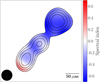 |
Fig. 10. Quasi-simultaneous spectral index map of OJ 287 between 86 GHz and 230 GHz. The 86 GHz data are from GMVA + ALMA observations taken on April 2, 2017 (Zhao et al. 2022). Both frequency maps were convolved with a 40 μas circular beam, as indicated in the bottom-left corner of the plot, corresponding to the resolution of the GMVA + ALMA observations. |
OJ 287 was observed for the first time with ALMA participating in the 3 mm GMVA array on April 2, 2017, just two days before our EHT observations (Zhao et al. 2022). The quasi-simultaneity of these observations allowed us to compare features in the C3*/P3* region and compute the spectral index map between 1.3 and 3.5 mm. As shown in Figure 10, the spectral index of the inner jet ranges from −0.7 to 0.3 (S ∝ ν+α), with the southeastern component C0 exhibiting a flat spectrum (α ∼ 0), consistent with its identification as the millimeter jet core. Downstream components display steeper spectra (α < 0), typical of optically thin jet regions.
The peculiar EVPAs and high degrees of polarization observed in P3* resemble those seen in the GMVA + ALMA observations, indicating a highly structured magnetic field and suggesting the presence of recollimation shocks (Zhao et al. 2022). These shocks, resulting from interactions between jet plasma and pressure imbalances in the surrounding medium, can compress magnetic fields, enhance polarized emission, and produce distinct EVPA patterns and conical jet shapes (e.g., Gómez et al. 1997, 2016; Cawthorne et al. 2013; Mizuno et al. 2015). The observed jet bending in C3*, where the jet shifts eastward at lower frequencies (e.g., Cohen et al. 2018; Gómez et al. 2022), further supports this interpretation and indicates a complex interplay of shock-driven and geometric processes influencing the emission properties in these regions.
4.3. Jet swing and binary black hole models
OJ 287 is among the best-known candidates for hosting a supermassive binary black hole (SMBBH) system and is a potential source of gravitational waves (e.g., Valtonen et al. 2008; Laine et al. 2020; Komossa et al. 2023b, and references therein). The binary hypothesis has been particularly effective in explaining the quasi-periodic light curves. Different variants of binary SMBH scenarios offered different explanations for these optical flares which are proposed to be triggered either by the secondary black hole crossing the accretion disk of the primary or else by variable beaming of the jet.
The orbital motion of the binary system is expected to leave its imprint on the inner jet direction. A comparison between our EHT images and those taken in 2014 with the RadioAstron space VLBI mission (Gómez et al. 2022), which has comparable angular resolution, shows a ∼50° change in the position angle of the inner jet. Similar swings on annual timescales were also observed at longer wavelengths, including the GMVA + ALMA data (Zhao et al. 2022). This directional change aligns well with the findings and predictions of Britzen et al. (2018) and Britzen et al. (2023), who first discovered the correlation between PA changes and jet direction using archival 15 GHz data. A similar binary model was later applied by Dey et al. (2021) using archival VLBI data at 22, 43, and 86 GHz, based on the earlier Lehto & Valtonen (1996) model, which proposes a large primary SMBH mass and strong orbital precession. In contrast, the binary model proposed by Liu & Wu (2002) and the binary model of Britzen et al. (2018) and Britzen et al. (2023) suggest a smaller primary SMBH mass of ∼108 M⊙, a hypothesis confirmed by recent results from broad-band variability and spectroscopy (MOMO project: Komossa et al. 2023a,b) and in particular by a direct measurement of the primary SMBH mass from applying well-established scaling relations between SMBH mass and broad-line emission which gives 108 M⊙ (Komossa et al. 2023b). Alternative binary models (e.g. Valtaoja et al. 2000; Liu & Wu 2002), as well as non-binary models, might also explain the jet’s position angle swing over annual timescales. These include the Lense-Thirring effect due to misalignment between the black hole spin and the accretion disk (e.g., Liska et al. 2018, 2021; Laine et al. 2020), or jet instabilities, such as K-H or current-driven types, which could generate a helical structure in the jet (e.g., Mizuno et al. 2012; Vega-García et al. 2019; Fuentes et al. 2023).
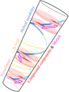 |
Fig. 11. Illustration of the proposed model for the jet structure in OJ 287. The helical magnetic field within the jet drives the formation of filamentary structures through K-H instabilities, which interact with plane-perpendicular shocks propagating downstream. These interactions enhance emission at specific locations, leading to the formation of distinct jet components observed in total intensity and polarization. Different features have a different color coding (see colors at the sides). |
4.4. Jet instabilities and shocks propagating through a jet threaded by a helical magnetic field
Our observations of OJ 287 show a twisted jet structure, prominently displayed in Figs. 4 and 8. This morphology initially suggests the possibility of a precessing jet, potentially caused by a binary black hole system or Lense-Thirring precession due to misalignment between the black hole’s spin axis and the accretion disk. In such precession models, we would expect jet components to move ballistically along paths altered by the precession-induced changes in jet direction. However, our observations indicate non-ballistic motions of the jet components, challenging the precession hypothesis as the sole explanation for the observed source morphology.
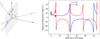 |
Fig. 12. (a, left) Geometry of the emission region, which moves with a velocity β, as seen in the source frame. Synchrotron radiation (electric field eobs) is emitted by relativistic electrons which move in a static magnetic field Bobs. The vector eobs (Bobs) makes an angle ξ (η) with the plane containing β and the observer direction n, and its projection on this plane makes an angle θ (ψ) with the z axis. Reproduced from Blandford & Königl (1979). (b, right) Observed polarization angle, ξ, measured clockwise from the projected jet axis computed for a jet with a bulk Lorentz factor of Γ = 10, viewing angle of 5.7° (i.e., roughly the critical angle 1/Γ), and threaded by a helical magnetic field with a pitch angle of αb = 89° (i.e., mostly toroidal). The time evolution of ξ is computed considering a K-H instability with a projected wavelength of 100 μas, and two perturbations moving at apparent velocities of 10.2 c and 17.4 c, to resemble observed components P1 and P2. The observed polarization angles of components P1 and P2, measured with respect to the jet axis, are also shown. |
An alternative explanation for the twisted jet ridgeline is the development of jet instabilities, specifically K-H instabilities (e.g., Hardee 2007). The fast proper motions we measure suggest that, at the scales probed by our observations (and further downstream), the jet is kinetically dominated–that is, the kinetic energy of the particles exceeds the magnetic energy. This kinetic dominance favors the growth of K-H instabilities, which arise from velocity shear between the jet and the surrounding medium. These instabilities can generate helical distortions that manifest as a twisted structure when projected onto the plane of the sky (e.g., Lobanov & Zensus 2001; Perucho et al. 2012; Cohen et al. 2015; Vega-García et al. 2019, 2020; Bruni et al. 2021).
The jet components we observe exhibit a relatively high degree of polarization, around 20%, and have well-defined magnetic homogeneous field orientations, except for component C3*, which appears to correspond to a recollimation shock. The high polarization observed in components C1/P1 and C2/P2 suggest that they correspond to shock waves traveling downstream within the jet (e.g., Marscher & Gear 1985; Gómez et al. 1997; Beuchert et al. 2018). Such moving shocks have been implicated in high-energy emission events, including the first detection of TeV γ-ray emission from OJ 287 (Lico et al. 2022, see also Subsection 4.2).
The observed twisted jet structure in OJ 287, along with the components’ high degree of polarization and evolving EVPAs, indicates a complex interplay between K-H instabilities and shocks in a jet threaded by a helical magnetic field. Figure 11 illustrates our proposed model, where K-H instabilities generate filamentary structures that interact with propagating shocks. These interactions compress the magnetic field and enhance emission in specific jet regions, explaining the distinct features observed in total intensity and polarization, as well as the rapid EVPA variations.
Previous polarization studies of OJ 287 by Cohen et al. (2018) and Cohen & Savolainen (2020) reported changes in the direction of EVPA rotation in integrated polarization measurements, which were interpreted as the superposition of a variable polarized component on top of a steady jet component. Other models, such as Marscher et al. (2008) for BL Lacertae, attribute EVPA rotations to components moving along helical trajectories, where the emitting region occupies only part of the jet cross-section. We emphasize that EVPA rotations in an axisymmetric jet require the emitting region to be confined to a localized section of the cross-section. In our model, while the moving shock spans the entire jet cross-section, enhanced emission arises from localized interactions with the helical filaments generated by K-H instabilities (see Figure 11). This allows the emitting region to probe varying azimuthal magnetic field structures as it propagates downstream, naturally producing EVPA rotations in the presence of a helical magnetic field. The interaction between the moving shocks and the helical K-H instability also naturally explains the observed non-ballistic apparent motions, even though the jet is straight. For the first time, high-resolution EHT data enable us to directly image these structures, providing concrete evidence of the interplay between jet instabilities, shocks, and helical magnetic fields.
Regarding the origin of the K-H wave, the modeled ridge-lines (see the April 10 ridgeline in Fig. 8) hint a periodical structure with a projected length of ∼100 μas. The corresponding de-projected length, assuming a viewing angle of ∼5° (e.g., Weaver et al. 2022), is therefore ∼ 5.3 pc. A simple translation into periodicity using the speed of light as the upper limit of the wave group velocity, results in a period ≳17 years in the source frame. This is of the order of the jet precession period reported in Britzen et al. (2018). It is possible, though, that the precession reported does not reveal a change in the direction of the PA of the whole jet, but only reveals the change in the ridge-line, as suggested in Perucho et al. (2012) for the quasar S5 0836+710, and confirmed by Lister et al. (2013) for sources monitored by the MOJAVE sample. Future work should aim to understand the coupling between the changes in the position angle of the observed jet and the trigger of the K-H instability, their physical origin, and weather these are the same at scales probed by the EHT and MOJAVE.
4.5. Modeling the time-variable structure in OJ 287
We now apply the previously described model (see also Figure 11) to analyze the time-variable structure observed in OJ 287, focusing particularly on the evolving EVPAs of its components. One of the most restrictive observational constraints is that components P1 and P2 exhibit EVPA rotations in opposite directions–counterclockwise for P1 and clockwise for P2.
When computing the observed synchrotron polarization, it is necessary to account for the characteristic swing in the polarization angle, as discussed previously in the seminal work by Blandford & Königl (1979) (see also Lyutikov et al. 2003). For a magnetic field, B, in the source frame, whose orientation is specified by the angles η and ψ, as shown in Figure 12, the observed polarization angle, ξ, is given by (Blandford & Königl 1979; Lyutikov et al. 2003)
 (3)
(3)
where βc is the velocity of the plasma and θ is the angle between β and the observer’s direction, n. Note that ξ is measured from the projected jet axis and is positive in the clockwise direction.
We could then compute how the polarization angle, ξ, evolves over time in our model. To do this, we considered a cylindrical jet (neglecting a small opening angle for simplicity) threaded by a helical magnetic field with a given pitch angle, αb, defined as the angle between the magnetic field and the jet axis. The helical magnetic field, measured in the source frame and normalized to unit strength, is expressed in Cartesian coordinates as
 (4)
(4)
where ϕ is the phase of the helical field.
To determine how ϕ evolves over time, we consider a helical K-H instability propagating along the jet surface with a projected wavelength of θλ ∼ 100 μas, as estimated previously. For simplicity, we neglect the rotation of the K-H instability over the 5-day time span of our observations. A plane-perpendicular shock travels along the jet with an apparent velocity βapp. The interaction of these moving shocks with the K-H instabilities gives rise to components P1 and P2, as observed (see Figure 11), and determines the evolution of ϕ and, consequently, the observed polarization angle ξ over time.
The phase of the helical magnetic field, ϕ, as a function of the observed time, tobs, is given by
 (5)
(5)
where ϕ0 is an arbitrary initial phase. Substituting this phase into the helical magnetic field expression (Equation (4)). Using Equation (3), where η = arcsin(−By) and ψ = arctan(Bx/Bz), we could obtain the observed polarization angle as a function of time.
Figure 12 shows the simulated time evolution of the polarization angle for components P1 and P2, assuming that the jet in OJ 287 is threaded by a predominantly toroidal magnetic field and is observed at an angle of approximately 1/Γ, with Γ being the jet’s bulk flow Lorentz factor. Due to light aberration, this viewing angle makes the line of sight nearly perpendicular to the jet axis in the plasma frame, leading to EVPAs that are more closely aligned with the jet axis for a predominantly toroidal magnetic field. (See the figure caption for the specific values used in our simulation.)
By examining Figure 12, we observe that, by assuming different initial phases in the magnetic field probed by each component, our model qualitatively reproduces the most salient observational feature: the opposite-direction rotation of the polarization angle in components P1 and P2. This effect occurs when the line of sight in the plasma frame exceeds the pitch angle of the magnetic field. Otherwise, a progressive evolution of the EVPAs is expected as the interaction of the component with the helical instability probes different phases of the helical magnetic field. As discussed in Blandford & Königl (1979), a rapid swing in the polarization angle is expected when β ∼ (cos θ − sin θ tan ψ), which can be tested in the future with more continuous and densely time sampled monitoring of the source.
Although our model can roughly reproduce the observed evolution of the polarization angle in P1 and P2, we note that it is not intended to exactly match the specific values of the observed EVPAs, as any combination of the Lorentz factor and viewing angle satisfying θ = 1/Γ would lead to similar rotations. Additionally, we have made several simplifications, such as assuming a perfectly straight jet with a perfectly helical instability, which is unlikely to hold in reality. Moreover, the model naturally accounts for the more rapid polarization rotation observed in the faster moving component.
Alternative models have explained blazar variability as the result of orientation changes of emitting regions in a twisting jet, which modulate the Doppler factor over time (e.g., Raiteri et al. 2017). In contrast, in our case the jet is straight and viewed at a constant angle, and the observed variability can be explained without invoking time-dependent Doppler factors. Instead, the EVPA rotations and apparent non-ballistic motions arise naturally from the interaction between plane perpendicular shocks and a helical Kelvin–Helmholtz instability in a jet threaded by a helical magnetic field.
On parsec scales, space–VLBI imaging with RadioAstron at 22 GHz, combined with multi-epoch VLBA observations at 43 GHz, revealed a ribbon-like inner jet in OJ 287 and multi-year swings of the jet position angle, consistent with a rotating helical Kelvin–Helmholtz pattern (Traianou et al. 2025), as envisioned in our model. Our EHT observations probe the jet much closer to its origin with tens of μas resolution at 230 GHz and follow its evolution over only a few days in April 2017. Together these data sets provide complementary perspectives, with RadioAstron and the VLBA tracing the parsec-scale multi-year evolution and the EHT capturing the rapid day-scale dynamics at the innermost jet base.
Previous observations of rapid optical polarization rotations in BL Lac by Marscher et al. (2008) inferred the presence of a helical magnetic field in the jet’s collimation and acceleration zone. However, the lack of angular resolution prevented a direct imaging of this effect, leaving its interpretation dependent on time-resolved polarization variability. Similarly, Cohen et al. (2018) and Cohen & Savolainen (2020) reported changes in the direction of EVPA rotation in integrated polarization measurements of OJ 287. Their model attributes these changes to the superposition of a variable polarized component on top of a steady jet component, which can produce apparent rotations in opposite directions when combined. In contrast, our EHT observations at an angular resolution of 18 μas for the first time is capable of directly resolving two distinct jet components, each exhibiting EVPA rotations in opposite directions. This spatially resolved evidence rules out the model based on integrated polarization components and provides direct support for the existence of a helical magnetic field in the jet’s collimation and acceleration zone. The ability to directly resolve these structures with EHT’s unprecedented angular resolution offers new constraints on jet formation, magnetic field evolution, and the role of instabilities in shaping AGN jets at their earliest stages.
5. Summary
We report on the first 1.3 mm observations of the candidate SMBH OJ 287 conducted with the EHT, which achieved an exceptional angular resolution of 18 μas. These observations reveal notable changes in both structural and polarization properties within just five days–the shortest interval over which such variability has been spatially resolved in this source.
The total intensity images reveal a twisted ridgeline structure extending northwest, with jet features displaying apparent superluminal motions reaching velocities up to ∼22 c. These rapid structural variations are also clearly visible in the evolving morphology of the jet ridgeline observed between the two epochs.
Polarimetric imaging identifies three prominent polarized components within the jet, and they show significant evolution in their EVPAs across the five-day interval. One component, located approximately 200 μas northwest from the core, exhibits a radial polarization signature consistent with a recollimation shock.
The observations directly resolve two innermost jet components exhibiting opposite directions of EVPA rotation: the faster-moving component (∼17.4 c) experiences counterclockwise rotations at ∼3.7° per day, whereas the slower-moving component (∼10.2 c) rotates clockwise at ∼2.5° per day. This result provides the first spatially resolved confirmation of a helical magnetic field threading the jet’s collimation and acceleration zones, which were previously inferred but not directly imaged in AGN jets.
The observed polarization variability is best explained by propagating shocks interacting with K-H instabilities, illuminating different phases of a threaded helical magnetic field. This interpretation rules out scenarios based solely on the blending of unresolved polarized components, emphasizing the crucial role of ordered magnetic field structures in driving the observed EVPA swings.
In addition, these millimeter-wavelength observations establish a compelling link to the historically observed highly variable optical polarization behavior in OJ 287. They suggest a common physical mechanism driving polarization variability across different wavelengths.
Acknowledgments
The motivation for the EHT observations originates from an initial proposal led by Gómez (PI), with significant contributions from Krichbaum and Komossa, alongside other coauthors. YYK was supported by the MuSES project, which has received funding from the European Union (ERC grant agreement No 101142396). Views and opinions expressed are however those of the author(s) only and do not necessarily reflect those of the European Union or ERCEA. Neither the European Union nor the granting authority can be held responsible for them. The Event Horizon Telescope Collaboration thanks the following organizations and programs: the Academia Sinica; the Academy of Finland (projects 274477, 284495, 312496, 315721); the Agencia Nacional de Investigación y Desarrollo (ANID), Chile via NCN19_058 (TITANs), Fondecyt 1221421 and BASAL FB210003; the Alexander von Humboldt Stiftung; an Alfred P. Sloan Research Fellowship; Allegro, the European ALMA Regional Centre node in the Netherlands, the NL astronomy research network NOVA and the astronomy institutes of the University of Amsterdam, Leiden University, and Radboud University; the ALMA North America Development Fund; the Astrophysics and High Energy Physics programme by MCIN (with funding from European Union NextGenerationEU, PRTR-C17I1); the Black Hole Initiative, which is funded by grants from the John Templeton Foundation (60477, 61497, 62286) and the Gordon and Betty Moore Foundation (Grant GBMF-8273) – although the opinions expressed in this work are those of the author and do not necessarily reflect the views of these Foundations; the Brinson Foundation; the Canada Research Chairs (CRC) program; Chandra DD7-18089X and TM6-17006X; the China Scholarship Council; the China Postdoctoral Science Foundation fellowships (2020M671266, 2022M712084); ANID through Fondecyt Postdoctorado (project 3250762); Conicyt through Fondecyt Postdoctorado (project 3220195); Consejo Nacional de Humanidades, Ciencia y Tecnología (CONAHCYT, Mexico, projects U0004-246083, U0004-259839, F0003-272050, M0037-279006, F0003-281692, 104497, 275201, 263356, CBF2023-2024-1102, 257435); the Colfuturo Scholarship; the Delaney Family via the Delaney Family John A. Wheeler Chair at Perimeter Institute; Dirección General de Asuntos del Personal Académico-Universidad Nacional Autónoma de México (DGAPA-UNAM, projects IN112820 and IN108324); the Dutch Research Council (NWO) for the VICI award (grant 639.043.513), the grant OCENW.KLEIN.113, and the Dutch Black Hole Consortium (with project No. NWA 1292.19.202) of the research programme the National Science Agenda; the Dutch National Supercomputers, Cartesius and Snellius (NWO grant 2021.013); the EACOA Fellowship awarded by the East Asia Core Observatories Association, which consists of the Academia Sinica Institute of Astronomy and Astrophysics, the National Astronomical Observatory of Japan, Center for Astronomical Mega-Science, Chinese Academy of Sciences, and the Korea Astronomy and Space Science Institute; the European Research Council (ERC) Synergy Grant “BlackHoleCam: Imaging the Event Horizon of Black Holes” (grant 610058) and Synergy Grant “BlackHolistic: Colour Movies of Black Holes: Understanding Black Hole Astrophysics from the Event Horizon to Galactic Scales” (grant 10107164); the European Union Horizon 2020 research and innovation programme under grant agreements RadioNet (No. 730562), M2FINDERS (No. 101018682) and FunFiCO (No. 777740); the European Research Council for advanced grant “JETSET: Launching, propagation and emission of relativistic jets from binary mergers and across mass scales” (grant No. 884631); the European Horizon Europe staff exchange (SE) programme HORIZON-MSCA-2021-SE-01 grant NewFunFiCO (No. 10108625); the Horizon ERC Grants 2021 programme under grant agreement No. 101040021; the FAPESP (Fundação de Amparo á Pesquisa do Estado de São Paulo) under grant 2021/01183-8; the Fondes de Recherche Nature et Technologies (FRQNT); the Fondo CAS-ANID folio CAS220010; the Generalitat Valenciana (grants APOSTD/2018/177 and ASFAE/2022/018) and GenT Program (project CIDEGENT/2018/021); the Gordon and Betty Moore Foundation (GBMF-3561, GBMF-5278, GBMF-10423); the Institute for Advanced Study; the ICSC – Centro Nazionale di Ricerca in High Performance Computing, Big Data and Quantum Computing, funded by European Union – NextGenerationEU; the Istituto Nazionale di Fisica Nucleare (INFN) sezione di Napoli, iniziative specifiche TEONGRAV; the International Max Planck Research School for Astronomy and Astrophysics at the Universities of Bonn and Cologne; the Italian Ministry of University and Research (MUR)– Project CUP F53D23001260001, funded by the European Union – NextGenerationEU; DFG research grant “Jet physics on horizon scales and beyond” (grant No. 443220636); Joint Columbia/Flatiron Postdoctoral Fellowship (research at the Flatiron Institute is supported by the Simons Foundation); the Japan Ministry of Education, Culture, Sports, Science and Technology (MEXT; grant JPMXP1020200109); the Japan Society for the Promotion of Science (JSPS) Grant-in-Aid for JSPS Research Fellowship (JP17J08829); the Joint Institute for Computational Fundamental Science, Japan; the Key Research Program of Frontier Sciences, Chinese Academy of Sciences (CAS, grants QYZDJ-SSW-SLH057, QYZDJSSW-SYS008, ZDBS-LY-SLH011); the Leverhulme Trust Early Career Research Fellowship; the Max-Planck-Gesellschaft (MPG); the Max Planck Partner Group of the MPG and the CAS; the MEXT/JSPS KAKENHI (grants 18KK0090, JP21H01137, JP18H03721, JP18K13594, 18K03709, JP19K14761, 18H01245, 25120007, 19H01943, 21H01137, 21H04488, 22H00157, 23K03453); the MICINN Research Projects PID2019-108995GB-C22, PID2022-140888NB-C22; the MIT International Science and Technology Initiatives (MISTI) Funds; the Ministry of Science and Technology (MOST) of Taiwan (103-2119-M-001-010-MY2, 105-2112-M-001-025-MY3, 105-2119-M-001-042, 106-2112-M-001-011, 106-2119-M-001-013, 106-2119-M-001-027, 106-2923-M-001-005, 107-2119-M-001-017, 107-2119-M-001-020, 107-2119-M-001-041, 107-2119-M-110-005, 107-2923-M-001-009, 108-2112-M-001-048, 108-2112-M-001-051, 108-2923-M-001-002, 109-2112-M-001-025, 109-2124-M-001-005, 109-2923-M-001-001, 110-2112-M-001-033, 110-2124-M-001-007 and 110-2923-M-001-001); the National Science and Technology Council (NSTC) of Taiwan (111-2124-M-001-005, 112-2124-M-001-014 and 112-2112-M-003-010-MY3); the Ministry of Education (MoE) of Taiwan Yushan Young Scholar Program; the Physics Division, National Center for Theoretical Sciences of Taiwan; the National Aeronautics and Space Administration (NASA, Fermi Guest Investigator grant 80NSSC23K1508, NASA Astrophysics Theory Program grant 80NSSC20K0527, NASA NuSTAR award 80NSSC20K0645); NASA Hubble Fellowship Program Einstein Fellowship; NASA Hubble Fellowship grants HST-HF2-51431.001-A, HST-HF2-51482.001-A, HST-HF2-51539.001-A, HST-HF2-51552.001A awarded by the Space Telescope Science Institute, which is operated by the Association of Universities for Research in Astronomy, Inc., for NASA, under contract NAS5-26555; the National Institute of Natural Sciences (NINS) of Japan; the National Key Research and Development Program of China (grant 2016YFA0400704, 2017YFA0402703, 2016YFA0400702); the National Science and Technology Council (NSTC, grants NSTC 111-2112-M-001 -041, NSTC 111-2124-M-001-005, NSTC 112-2124-M-001-014); the US National Science Foundation (NSF, grants AST-0096454, AST-0352953, AST-0521233, AST-0705062, AST-0905844, AST-0922984, AST-1126433, OIA-1126433, AST-1140030, DGE-1144085, AST-1207704, AST-1207730, AST-1207752, MRI-1228509, OPP-1248097, AST-1310896, AST-1440254, AST-1555365, AST-1614868, AST-1615796, AST-1715061, AST-1716327, AST-1726637, OISE-1743747, AST-1743747, AST-1816420, AST-1935980, AST-1952099, AST-2034306, AST-2205908, AST-2307887); NSF Astronomy and Astrophysics Postdoctoral Fellowship (AST-1903847); the Natural Science Foundation of China (grants 11650110427, 10625314, 11721303, 11725312, 11873028, 11933007, 11991052, 11991053, 12192220, 12192223, 12273022, 12325302, 12303021); the Natural Sciences and Engineering Research Council of Canada (NSERC); the National Research Foundation of Korea (the Global PhD Fellowship Grant: grants NRF-2015H1A2A1033752; the Korea Research Fellowship Program: NRF-2015H1D3A1066561; Brain Pool Program: RS-2024-00407499; Basic Research Support Grant 2019R1F1A1059721, 2021R1A6A3A01086420, 2022R1C1C1005255, 2022R1F1A1075115); Netherlands Research School for Astronomy (NOVA) Virtual Institute of Accretion (VIA) postdoctoral fellowships; NOIRLab, which is managed by the Association of Universities for Research in Astronomy (AURA) under a cooperative agreement with the National Science Foundation; Onsala Space Observatory (OSO) national infrastructure, for the provisioning of its facilities/observational support (OSO receives funding through the Swedish Research Council under grant 2017-00648); the Perimeter Institute for Theoretical Physics (research at Perimeter Institute is supported by the Government of Canada through the Department of Innovation, Science and Economic Development and by the Province of Ontario through the Ministry of Research, Innovation and Science); the Portuguese Foundation for Science and Technology (FCT) grants (Individual CEEC program – 5th edition, https://doi.org/10.54499/UIDB/04106/2020, https://doi.org/10.54499/UIDP/04106/2020, PTDC/FIS-AST/3041/2020, CERN/FIS-PAR/0024/2021, 2022.04560.PTDC); the Princeton Gravity Initiative; the Spanish Ministerio de Ciencia, Innovación y Universidades (grants PID2022-140888NB-C21, PID2022-140888NB-C22, PID2023-147883NB-C21, RYC2023-042988-I); the Severo Ochoa grant CEX2021-001131-S funded by MICIU/AEI/10.13039/501100011033; The European Union’s Horizon Europe research and innovation program under grant agreement No. 101093934 (RADIOBLOCKS); The European Union “NextGenerationEU”, the Recovery, Transformation and Resilience Plan, the CUII of the Andalusian Regional Government and the Spanish CSIC through grant AST22_00001_Subproject_10; “la Caixa” Foundation (ID 100010434) through fellowship codes LCF/BQ/DI22/11940027 and LCF/BQ/DI22/11940030; the University of Pretoria for financial aid in the provision of the new Cluster Server nodes and SuperMicro (USA) for a SEEDING GRANT approved toward these nodes in 2020; the Shanghai Municipality orientation program of basic research for international scientists (grant no. 22JC1410600); the Shanghai Pilot Program for Basic Research, Chinese Academy of Science, Shanghai Branch (JCYJ-SHFY-2021-013); the Simons Foundation (grant 00001470); the Spanish Ministry for Science and Innovation grant CEX2021-001131-S funded by MCIN/AEI/10.13039/501100011033; the Spinoza Prize SPI 78-409; the South African Research Chairs Initiative, through the South African Radio Astronomy Observatory (SARAO, grant ID 77948), which is a facility of the National Research Foundation (NRF), an agency of the Department of Science and Innovation (DSI) of South Africa; the Swedish Research Council (VR); the Taplin Fellowship; the Toray Science Foundation; the UK Science and Technology Facilities Council (grant no. ST/X508329/1); the US Department of Energy (USDOE) through the Los Alamos National Laboratory (operated by Triad National Security, LLC, for the National Nuclear Security Administration of the USDOE, contract 89233218CNA000001); and the YCAA Prize Postdoctoral Fellowship. This work was also supported by the National Research Foundation of Korea (NRF) grant funded by the Korea government(MSIT) (RS-2024-00449206). We acknowledge support from the Coordenação de Aperfeiçoamento de Pessoal de Nível Superior (CAPES) of Brazil through PROEX grant number 88887.845378/2023-00. We acknowledge financial support from Millenium Nucleus NCN23_002 (TITANs) and Comité Mixto ESO-Chile. We thank the staff at the participating observatories, correlation centers, and institutions for their enthusiastic support. ALMA is a partnership of the European Southern Observatory (ESO; Europe, representing its member states), NSF, and National Institutes of Natural Sciences of Japan, together with National Research Council (Canada), Ministry of Science and Technology (MOST; Taiwan), Academia Sinica Institute of Astronomy and Astrophysics (ASIAA; Taiwan), and Korea Astronomy and Space Science Institute (KASI; Republic of Korea), in cooperation with the Republic of Chile. The Joint ALMA Observatory is operated by ESO, Associated Universities, Inc. (AUI)/NRAO, and the National Astronomical Observatory of Japan (NAOJ). The NRAO is a facility of the NSF operated under cooperative agreement by AUI. This research used resources of the Oak Ridge Leadership Computing Facility at the Oak Ridge National Laboratory, which is supported by the Office of Science of the U.S. Department of Energy under contract No. DE-AC05-00OR22725; the ASTROVIVES FEDER infrastructure, with project code IDIFEDER-2021-086; the computing cluster of Shanghai VLBI correlator supported by the Special Fund for Astronomy from the Ministry of Finance in China; We also thank the Center for Computational Astrophysics, National Astronomical Observatory of Japan. This work was supported by FAPESP (Fundacao de Amparo a Pesquisa do Estado de Sao Paulo) under grant 2021/01183-8. APEX is a collaboration between the Max-Planck-Institut für Radioastronomie (Germany), ESO, and the Onsala Space Observatory (Sweden). The SMA is a joint project between the SAO and ASIAA and is funded by the Smithsonian Institution and the Academia Sinica. The JCMT is operated by the East Asian Observatory on behalf of the NAOJ, ASIAA, and KASI, as well as the Ministry of Finance of China, Chinese Academy of Sciences, and the National Key Research and Development Program (No. 2017YFA0402700) of China and Natural Science Foundation of China grant 11873028. Additional funding support for the JCMT is provided by the Science and Technologies Facility Council (UK) and participating universities in the UK and Canada. The LMT is a project operated by the Instituto Nacional de Astrófisica, Óptica, y Electrónica (Mexico) and the University of Massachusetts at Amherst (USA). The IRAM 30-m telescope on Pico Veleta, Spain is operated by IRAM and supported by CNRS (Centre National de la Recherche Scientifique, France), MPG (Max-Planck-Gesellschaft, Germany), and IGN (Instituto Geográfico Nacional, Spain). The SMT is operated by the Arizona Radio Observatory, a part of the Steward Observatory of the University of Arizona, with financial support of operations from the State of Arizona and financial support for instrumentation development from the NSF. Support for SPT participation in the EHT is provided by the National Science Foundation through award OPP-1852617 to the University of Chicago. Partial support is also provided by the Kavli Institute of Cosmological Physics at the University of Chicago. The SPT hydrogen maser was provided on loan from the GLT, courtesy of ASIAA. This work used the Extreme Science and Engineering Discovery Environment (XSEDE), supported by NSF grant ACI-1548562, and CyVerse, supported by NSF grants DBI-0735191, DBI-1265383, and DBI-1743442. XSEDE Stampede2 resource at TACC was allocated through TG-AST170024 and TG-AST080026N. XSEDE JetStream resource at PTI and TACC was allocated through AST170028. This research is part of the Frontera computing project at the Texas Advanced Computing Center through the Frontera Large-Scale Community Partnerships allocation AST20023. Frontera is made possible by National Science Foundation award OAC-1818253. This research was done using services provided by the OSG Consortium (Pordes et al. 2007; Sfiligoi et al. 2009), which is supported by the National Science Foundation award Nos. 2030508 and 1836650. Additional work used ABACUS2.0, which is part of the eScience center at Southern Denmark University, and the Kultrun Astronomy Hybrid Cluster (projects Conicyt Programa de Astronomia Fondo Quimal QUIMAL170001, Conicyt PIA ACT172033, Fondecyt Iniciacion 11170268, Quimal 220002). Simulations were also performed on the SuperMUC cluster at the LRZ in Garching, on the LOEWE cluster in CSC in Frankfurt, on the HazelHen cluster at the HLRS in Stuttgart, and on the Pi2.0 and Siyuan Mark-I at Shanghai Jiao Tong University. The computer resources of the Finnish IT Center for Science (CSC) and the Finnish Computing Competence Infrastructure (FCCI) project are acknowledged. This research was enabled in part by support provided by Compute Ontario (http://computeontario.ca), Calcul Quebec (http://www.calculquebec.ca), and the Digital Research Alliance of Canada (https://alliancecan.ca/en). The EHTC has received generous donations of FPGA chips from Xilinx Inc., under the Xilinx University Program. The EHTC has benefited from technology shared under open-source license by the Collaboration for Astronomy Signal Processing and Electronics Research (CASPER). The EHT project is grateful to T4Science and Microsemi for their assistance with hydrogen masers. This research has made use of NASA’s Astrophysics Data System. We gratefully acknowledge the support provided by the extended staff of the ALMA, from the inception of the ALMA Phasing Project through the observational campaigns of 2017 and 2018. We would like to thank A. Deller and W. Brisken for EHT-specific support with the use of DiFX. We thank Martin Shepherd for the addition of extra features in the Difmap software that were used for the CLEAN imaging results presented in this paper. We acknowledge the significance that Maunakea, where the SMA and JCMT EHT stations are located, has for the indigenous Hawaiian people.
References
- Akiyama, K., Kuramochi, K., Ikeda, S., et al. 2017a, ApJ, 838, 1 [NASA ADS] [CrossRef] [Google Scholar]
- Akiyama, K., Ikeda, S., Pleau, M., et al. 2017b, AJ, 153, 159 [NASA ADS] [CrossRef] [Google Scholar]
- Baczko, A.-K., Kadler, M., Ros, E., et al. 2024, A&A, 692, A205 [NASA ADS] [CrossRef] [EDP Sciences] [Google Scholar]
- Beuchert, T., Kadler, M., Perucho, M., et al. 2018, A&A, 610, A32 [NASA ADS] [CrossRef] [EDP Sciences] [Google Scholar]
- Blackburn, L., Chan, C.-K., Crew, G. B., et al. 2019, ApJ, 882, 23 [Google Scholar]
- Blandford, R. D., & Königl, A. 1979, ApJ, 232, 34 [Google Scholar]
- Blandford, R. D., & Payne, D. G. 1982, MNRAS, 199, 883 [CrossRef] [Google Scholar]
- Blandford, R. D., & Znajek, R. L. 1977, MNRAS, 179, 433 [NASA ADS] [CrossRef] [Google Scholar]
- Britzen, S., Fendt, C., Witzel, G., et al. 2018, MNRAS, 478, 3199 [NASA ADS] [Google Scholar]
- Britzen, S., ZajačD;ek, M., Gopal-Krishna, et al. 2023, ApJ, 951, 106 [CrossRef] [Google Scholar]
- Broderick, A. E., Pesce, D. W., Tiede, P., Pu, H.-Y., & Gold, R. 2020a, ApJ, 898, 9 [Google Scholar]
- Broderick, A. E., Gold, R., Karami, M., et al. 2020b, ApJ, 897, 139 [Google Scholar]
- Bruni, G., Gómez, J. L., Vega-García, L., et al. 2021, A&A, 654, A27 [NASA ADS] [CrossRef] [EDP Sciences] [Google Scholar]
- Cawthorne, T. V., Jorstad, S. G., & Marscher, A. P. 2013, ApJ, 772, 14 [NASA ADS] [CrossRef] [Google Scholar]
- Chael, A. A., Johnson, M. D., Narayan, R., et al. 2016, ApJ, 829, 11 [Google Scholar]
- Chael, A. A., Johnson, M. D., Bouman, K. L., et al. 2018, ApJ, 857, 23 [Google Scholar]
- Cohen, M. H., & Savolainen, T. 2020, A&A, 636, A79 [NASA ADS] [CrossRef] [EDP Sciences] [Google Scholar]
- Cohen, M. H., Meier, D. L., Arshakian, T. G., et al. 2015, ApJ, 803, 3 [Google Scholar]
- Cohen, M. H., Aller, H. D., Aller, M. F., et al. 2018, ApJ, 862, 1 [NASA ADS] [CrossRef] [Google Scholar]
- Deller, A. T., Brisken, W. F., Phillips, C. J., et al. 2011, PASP, 123, 275 [Google Scholar]
- Dey, L., Valtonen, M. J., Gopakumar, A., et al. 2021, MNRAS, 503, 4400 [NASA ADS] [CrossRef] [Google Scholar]
- EHT MWL Science Working Group, Algaba, J. C., Anczarski, J., et al. 2021, ApJ, 911, L11 [NASA ADS] [CrossRef] [Google Scholar]
- Event Horizon Telescope Collaboration (Akiyama, K., et al.) 2019a, ApJ, 875, L1 (M87∗ Paper I) [Google Scholar]
- Event Horizon Telescope Collaboration (Akiyama, K., et al.) 2019b, ApJ, 875, L2 (M87∗ Paper II) [Google Scholar]
- Event Horizon Telescope Collaboration (Akiyama, K., et al.) 2019c, ApJ, 875, L3 (M87∗ Paper III) [Google Scholar]
- Event Horizon Telescope Collaboration (Akiyama, K., et al.) 2019d, ApJ, 875, L4 (M87∗ Paper IV) [Google Scholar]
- Event Horizon Telescope Collaboration (Akiyama, K., et al.) 2019e, ApJ, 875, L5 (M87∗ Paper V) [Google Scholar]
- Event Horizon Telescope Collaboration (Akiyama, K., et al.) 2019f, ApJ, 875, L6 (M87∗ Paper VI) [Google Scholar]
- Event Horizon Telescope Collaboration (Akiyama, K., et al.) 2021a, ApJ, 910, L12 (M87∗ Paper VII) [Google Scholar]
- Event Horizon Telescope Collaboration (Akiyama, K., et al.) 2021b, ApJ, 910, L13 (M87∗ Paper VIII) [Google Scholar]
- Event Horizon Telescope Collaboration (Akiyama, K., et al.) 2022a, ApJ, 930, L12 [NASA ADS] [CrossRef] [Google Scholar]
- Event Horizon Telescope Collaboration (Akiyama, K., et al.) 2022b, ApJ, 930, L13 [NASA ADS] [CrossRef] [Google Scholar]
- Event Horizon Telescope Collaboration (Akiyama, K., et al.) 2022c, ApJ, 930, L14 [NASA ADS] [CrossRef] [Google Scholar]
- Event Horizon Telescope Collaboration (Akiyama, K., et al.) 2022d, ApJ, 930, L15 [NASA ADS] [CrossRef] [Google Scholar]
- Event Horizon Telescope Collaboration (Akiyama, K., et al.) 2022e, ApJ, 930, L16 [NASA ADS] [CrossRef] [Google Scholar]
- Event Horizon Telescope Collaboration (Akiyama, K., et al.) 2022f, ApJ, 930, L17 [NASA ADS] [CrossRef] [Google Scholar]
- Event Horizon Telescope Collaboration (Akiyama, K., et al.) 2023, ApJ, 957, L20 [NASA ADS] [CrossRef] [Google Scholar]
- Event Horizon Telescope Collaboration (Akiyama, K., et al.) 2024a, ApJ, 964, L25 [NASA ADS] [CrossRef] [Google Scholar]
- Event Horizon Telescope Collaboration (Akiyama, K., et al.) 2024b, ApJ, 964, L26 [CrossRef] [Google Scholar]
- Farris, B. D., Gold, R., Paschalidis, V., Etienne, Z. B., & Shapiro, S. L. 2012, Phys. Rev. Lett., 109, 221102 [Google Scholar]
- Fuentes, A., Gómez, J. L., Martí, J. M., et al. 2023, Nat. Astron., 7, 1359 [NASA ADS] [CrossRef] [Google Scholar]
- Goddi, C., Martí-Vidal, I., Messias, H., et al. 2019, PASP, 131, 075003 [Google Scholar]
- Goddi, C., Martí-Vidal, I., Messias, H., et al. 2021, ApJ, 910, L14 [NASA ADS] [CrossRef] [Google Scholar]
- Gold, R. 2019, Galaxies, 7, 63 [Google Scholar]
- Gold, R., Paschalidis, V., Etienne, Z. B., Shapiro, S. L., & Pfeiffer, H. P. 2014a, Phys. Rev. D, 89, 064060 [NASA ADS] [CrossRef] [Google Scholar]
- Gold, R., Paschalidis, V., Ruiz, M., et al. 2014b, Phys. Rev. D, 90, 104030 [NASA ADS] [CrossRef] [Google Scholar]
- Gómez, J. L., Martí, J. M., Marscher, A. P., Ibááñez, J. M., & Alberdi, A. 1997, ApJ, 482, L33 [CrossRef] [Google Scholar]
- Gómez, J. L., Lobanov, A. P., Bruni, G., et al. 2016, ApJ, 817, 96 [Google Scholar]
- Gómez, J. L., Traianou, E., Krichbaum, T. P., et al. 2022, ApJ, 924, 122 [Google Scholar]
- Grupe, D., Komossa, S., & Gomez, J. L. 2016, ATel, 9629, 1 [Google Scholar]
- Grupe, D., Komossa, S., & Falcone, A. 2017, ATel, 10043, 1 [Google Scholar]
- Hardee, P. E. 2007, ApJ, 664, 26 [Google Scholar]
- Hodgson, J. A., Krichbaum, T. P., Marscher, A. P., et al. 2017, A&A, 597, A80 [NASA ADS] [CrossRef] [EDP Sciences] [Google Scholar]
- Issaoun, S., Wielgus, M., Jorstad, S., et al. 2022, ApJ, 934, 145 [NASA ADS] [CrossRef] [Google Scholar]
- Janssen, M., Goddi, C., van Bemmel, I. M., et al. 2019, A&A, 626, A75 [NASA ADS] [CrossRef] [EDP Sciences] [Google Scholar]
- Janssen, M., Falcke, H., Kadler, M., et al. 2021, Nat. Astron., 5, 1017 [NASA ADS] [CrossRef] [Google Scholar]
- Janssen, M., Radcliffe, J. F., & Wagner, J. 2022, Universe, 8, 527 [NASA ADS] [CrossRef] [Google Scholar]
- Jorstad, S., & Marscher, A. 2016, Galaxies, 4, 47 [Google Scholar]
- Jorstad, S. G., Marscher, A. P., Lister, M. L., et al. 2005, AJ, 130, 1418 [Google Scholar]
- Jorstad, S. G., Marscher, A. P., Larionov, V. M., et al. 2010, ApJ, 715, 362 [Google Scholar]
- Jorstad, S. G., Marscher, A. P., Morozova, D. A., et al. 2017, ApJ, 846, 98 [Google Scholar]
- Jorstad, S. G., Marscher, A. P., Raiteri, C. M., et al. 2022, Nature, 609, 265 [NASA ADS] [CrossRef] [Google Scholar]
- Jorstad, S., Wielgus, M., Lico, R., et al. 2023, ApJ, 943, 170 [NASA ADS] [CrossRef] [Google Scholar]
- Kim, J.-Y., Krichbaum, T. P., Broderick, A. E., et al. 2020, A&A, 640, A69 [EDP Sciences] [Google Scholar]
- Komossa, S., Grupe, D., Schartel, N., et al. 2017, in New Frontiers in Black Hole Astrophysics, ed. A. Gomboc, IAU Symp., 324, 168 [NASA ADS] [Google Scholar]
- Komossa, S., Grupe, D., Parker, M. L., et al. 2020, MNRAS, 498, L35 [NASA ADS] [CrossRef] [Google Scholar]
- Komossa, S., Grupe, D., Gallo, L. C., et al. 2021b, ApJ, 923, 51 [Google Scholar]
- Komossa, S., Grupe, D., Parker, M. L., et al. 2021a, MNRAS, 504, 5575 [NASA ADS] [CrossRef] [Google Scholar]
- Komossa, S., Grupe, D., Kraus, A., et al. 2023a, MNRAS, 522, L84 [NASA ADS] [CrossRef] [Google Scholar]
- Komossa, S., Kraus, A., Grupe, D., et al. 2023b, ApJ, 944, 177 [NASA ADS] [CrossRef] [Google Scholar]
- Laine, S., Dey, L., Valtonen, M., et al. 2020, ApJ, 894, L1 [NASA ADS] [CrossRef] [Google Scholar]
- Lehto, H. J., & Valtonen, M. J. 1996, ApJ, 460, 207 [NASA ADS] [CrossRef] [Google Scholar]
- Lico, R., Casadio, C., Jorstad, S. G., et al. 2022, A&A, 658, L10 [NASA ADS] [CrossRef] [EDP Sciences] [Google Scholar]
- Liska, M., Hesp, C., Tchekhovskoy, A., et al. 2018, MNRAS, 474, L81 [Google Scholar]
- Liska, M., Hesp, C., Tchekhovskoy, A., et al. 2021, MNRAS, 507, 983 [NASA ADS] [CrossRef] [Google Scholar]
- Lister, M. L., Aller, M. F., Aller, H. D., et al. 2013, AJ, 146, 120 [Google Scholar]
- Lister, M. L., Aller, M. F., Aller, H. D., et al. 2018, ApJS, 234, 12 [CrossRef] [Google Scholar]
- Liu, F. K., & Wu, X. B. 2002, A&A, 388, L48 [NASA ADS] [CrossRef] [EDP Sciences] [Google Scholar]
- Lobanov, A. P., & Zensus, J. A. 2001, Science, 294, 128 [Google Scholar]
- Lyutikov, M., Pariev, V. I., & Blandford, R. D. 2003, ApJ, 597, 998 [Google Scholar]
- Marscher, A. P. 2014, ApJ, 780, 87 [Google Scholar]
- Marscher, A. P., & Gear, W. K. 1985, ApJ, 298, 114 [Google Scholar]
- Marscher, A. P., Jorstad, S. G., D’Arcangelo, F. D., et al. 2008, Nature, 452, 966 [Google Scholar]
- Martí-Vidal, I., Vlemmings, W. H. T., & Muller, S. 2016, A&A, 593, A61 [NASA ADS] [CrossRef] [EDP Sciences] [Google Scholar]
- Mizuno, Y., Lyubarsky, Y., Nishikawa, K.-I., & Hardee, P. E. 2012, ApJ, 757, 16 [Google Scholar]
- Mizuno, Y., Gómez, J. L., Nishikawa, K.-I., et al. 2015, ApJ, 809, 38 [Google Scholar]
- Mukherjee, R., & VERITAS Collaboration. 2017, ATel, 10051, 1 [Google Scholar]
- Müller, H., & Lobanov, A. P. 2022, A&A, 666, A137 [NASA ADS] [CrossRef] [EDP Sciences] [Google Scholar]
- Nakamura, M., Li, H., & Li, S. 2007, ApJ, 656, 721 [NASA ADS] [CrossRef] [Google Scholar]
- O’Brien, S. 2017, ArXiv e-prints [arXiv:1708.02160] [Google Scholar]
- Paraschos, G. F., Kim, J. Y., Wielgus, M., et al. 2024, A&A, 682, L3 [NASA ADS] [CrossRef] [EDP Sciences] [Google Scholar]
- Paschalidis, V., Bright, J., Ruiz, M., & Gold, R. 2021, ApJ, 910, L26 [Google Scholar]
- Perucho, M., Hanasz, M., Martí, J. M., & Miralles, J. A. 2004, A&A, 427, 415 [NASA ADS] [CrossRef] [EDP Sciences] [Google Scholar]
- Perucho, M., Kovalev, Y. Y., Lobanov, A. P., Hardee, P. E., & Agudo, I. 2012, ApJ, 749, 55 [Google Scholar]
- Pesce, D. W. 2021, AJ, 161, 178 [NASA ADS] [CrossRef] [Google Scholar]
- Planck Collaboration VI. 2020, A&A, 641, A6 [NASA ADS] [CrossRef] [EDP Sciences] [Google Scholar]
- Pordes, R., Petravick, D., Kramer, B., et al. 2007, J. Phys.: Conf. Ser., 78, 012057 [CrossRef] [Google Scholar]
- Pushkarev, A. B., & Kovalev, Y. Y. 2012, A&A, 544, A34 [NASA ADS] [CrossRef] [EDP Sciences] [Google Scholar]
- Raiteri, C. M., Villata, M., Acosta-Pulido, J. A., et al. 2017, Nature, 552, 374 [NASA ADS] [CrossRef] [Google Scholar]
- Röder, J., Wielgus, M., Lobanov, A. P., et al. 2025, A&A, 695, A233 [NASA ADS] [CrossRef] [EDP Sciences] [Google Scholar]
- Schinzel, F. K., Lobanov, A. P., Taylor, G. B., et al. 2012, A&A, 537, 70 [Google Scholar]
- Sfiligoi, I., Bradley, D. C., Holzman, B., et al. 2009, in 2009 WRI World Congress on Computer Science and Information Engineering, 2 (Piscataway, NJ: IEEE), 428 [CrossRef] [Google Scholar]
- Shepherd, M. C. 1997, in Astronomical Data Analysis Software and Systems VI, eds. G. Hunt, & H. E. Payne (San Francisco: ASP), ASP Conf. Ser., 125, 77 [Google Scholar]
- Sillanpää, A., Haarala, S., Valtonen, M. J., Sundelius, B., & Byrd, G. G. 1988, ApJ, 325, 628 [NASA ADS] [CrossRef] [Google Scholar]
- Sironi, L., Keshet, U., & Lemoine, M. 2015, Space Sci. Rev., 191, 519 [CrossRef] [Google Scholar]
- Stickel, M., Fried, J. W., & Kuehr, H. 1989, A&AS, 80, 103 [NASA ADS] [Google Scholar]
- Traianou, E., Gómez, J. L., Cho, I., et al. 2025, A&A, 700, A16 [NASA ADS] [CrossRef] [EDP Sciences] [Google Scholar]
- Valtaoja, E., Teräsranta, H., Tornikoski, M., et al. 2000, ApJ, 531, 744 [NASA ADS] [CrossRef] [Google Scholar]
- Valtonen, M. J., Lehto, H. J., Nilsson, K., et al. 2008, Nature, 452, 851 [Google Scholar]
- Vega-García, L., Perucho, M., & Lobanov, A. P. 2019, A&A, 627, A79 [NASA ADS] [CrossRef] [EDP Sciences] [Google Scholar]
- Vega-García, L., Lobanov, A. P., Perucho, M., et al. 2020, A&A, 641, A40 [NASA ADS] [CrossRef] [EDP Sciences] [Google Scholar]
- Villata, M., Raiteri, C. M., Sillanpää, A., & Takalo, L. O. 1998, MNRAS, 293, L13 [NASA ADS] [CrossRef] [Google Scholar]
- Weaver, Z. R., Jorstad, S. G., Marscher, A. P., et al. 2022, ApJS, 260, 12 [NASA ADS] [CrossRef] [Google Scholar]
- Zhao, G.-Y., Gómez, J. L., Fuentes, A., et al. 2022, ApJ, 932, 72 [NASA ADS] [CrossRef] [Google Scholar]
Appendix A: Homogenizing the image resolution
The different pipelines used to image OJ287 produce images with a specific resolution, which varies from pipeline to pipeline. Therefore, we must take care in uniforming the resolution of the images when comparing them one to the other or when averaging them together. This section explains how we define the resolution of an image and what process we use to downgrade the resolution, in order to compare across images.
The resolution of an image is the smallest spatial scale at which there are variations in the image intensity. The resolution is limited, though not determined, by the number of pixels, as pixels can be arbitrarily added to an image without increasing the details present in it. The resolution of an image can also assume different values along different spatial directions. In particular, this is the case of DIFMAP images convolved with an elliptical beam. For an image I(x, y), we estimated the amplitude of the intensity variations at different spatial scales by computing its power spectrum P(k) of the image:
 (A.1)
(A.1)
which is the average over the angular coordinate in the image plane of the Fourier transform S(kx, ky),
 (A.2)
(A.2)
,
of the image autocorrelation function R(x, y):
 (A.3)
(A.3)
The power spectrum of an image has a significant drop at the scale corresponding to the image resolution, meaning that at smaller scales no intensity variation is present. Figure A.1 shows the images as given by each pipeline and their corresponding power spectra are plotted in Figure A.2 (top row panels). It is clear that DIFMAP is the image with the lowest resolution, since the corresponding power spectrum drops at larger scales, so we decided to downgrade the resolution of the other images to the DIFMAP one. To do so, we convolved the images with a Gaussian beam, choosing the full width at half maximum (FWHM) that resulted in the best fit between the power spectrum of the convolved image and the power spectrum of the DIFMAP image. We tested for values of the circular Gaussian with a FWHM ranging from 0 to 47.04 μ as in intervals of 0.47 μ as. The best fit values are presented in Table A.1 for each pipeline and day.
Values of the circular Gaussian FWHM used to convolve the images to the same resolution as that of DIFMAP images.
The power spectra of the convolved images are shown in Figure A.2 (bottom row). After convolution, the drop in the power spectra is located at the same scale for all pipelines, meaning that they have the same resolution. The convolved images are presented in Figure 3.
It is to be noted that, since the power spectrum averages the amplitude of the fluctuations across all different directions, this method for estimating the resolution assumes that the resolution of the image is isotropic. We reckon that this will not represent an issue in our case, as the ellipticity of the DIFMAP beam is low (0.16 for April 5 and 0.13 for April 10).
After uniforming the resolution of the images from the different pipelines, both the total flux and the global image morphology are very similar across the images. Therefore, we averaged them together using equal weights to produce the final images of OJ 287 that we present in this paper.
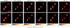 |
Fig. A.1. Total intensity images of OJ 287 on April 5 and 10 for different imaging pipelines without any convolution. The RML imaging methods are separated by a dashed black line while the Bayesian imaging methods are separated by a solid black line. The DIFMAP images are convolved with circular Gaussian of 18 μ as, corresponding to the maximum of the minor axes of the CLEAN beams (which are approximately circular) of April 5 and 10. |
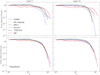 |
Fig. A.2. Top row: Power spectra of the images of different pipelines on April 5 and 10 in Fig. A.1 computed according to Equation A.1. Bottom row: Power spectra after convolving the images according to Table A.1. |
Appendix B: Image fidelity
As described in subsection 2.2, three different imaging approaches were employed: (1) inverse modeling, (2) forward modeling, and (3) Bayesian sampling based on forward models. The CLEAN algorithm, implemented in the DIFMAP software, was used for inverse modeling, while the RML method was applied using eht-imaging, SMILI, and DoG-HiT for forward modeling. In both cases, a parameter search was conducted to identify a fiducial image, with parameters optimized to achieve a reduced χ2 close to 1 for the closure quantities. In contrast, the Bayesian sampling methods THEMIS and DMC do not require a parameter search; instead, they produce a posterior distribution directly.
As a result, images from six methods were obtained, each fitting the various combinations of closure triangles and quadrangles effectively, as demonstrated for selected triangles and quadrangles in Figure B.1. It is worth noting that the models (solid lines) show some deviations in regions without data points. This is a natural consequence of the ill-posed nature of the inverse problem in interferometric imaging, where each image interpolates gaps based on the selected imaging parameters. Nevertheless, these deviations are not significant, as the models explain the data well and produce consistent images (Figure 3).
Three of the six pipelines—DIFMAP, DMC, and eht-imaging—were further utilized for polarization imaging, covering all three distinct imaging and modeling approaches. As with total intensity imaging, a parameter search was conducted for DIFMAP and eht-imaging, while DMC directly provided a posterior distribution. The resulting polarization features were consistent across all three methods (Figure B.2), allowing us to reasonably average these features to produce the final polarization map shown in Figure 4.
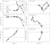 |
Fig. B.1. Closure phases (left) and log closure amplitudes (right) for selected triangles and quadrangles plotted as a function of observing time. The stations forming each triangle or quadrangle are indicated in the top-left corner of each panel. Closure quantities derived from the imaging and modeling results are shown in different colors, demonstrating a good fit to the data. The shaded areas indicate the uncertainty range or variability in the closure quantities. Filled circles represent results from April 5, while open squares correspond to April 10. The antenna codes correspond to AA (ALMA), AZ (Submillimeter Telescope), JC (James Clerk Maxwell Telescope), LM (Large Millimeter Telescope Alfonso Serrano), PV (IRAM 30 m Telescope), JC (James Clerk Maxwell Telescope), SM (Submillimeter Array). |
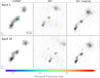 |
Fig. B.2. Polarimetric images of OJ 287, produced using DIFMAP, DMC, and eht-imaging. Total intensity emission is shown in grayscale, while white contours represent polarization intensity at levels of 25%, 50%, and 75% of the peak polarization intensity. Ticks indicate the orientation of the EVPA, with their length representing the magnitude of linear polarization intensity and their color denoting the fractional linear polarization. EVPAs are shown only where the total and linear polarization intensities exceed their respective noise thresholds, which are ∼0.3 mJy/beam for total intensity and ∼0.5 mJy/beam for linear polarized intensity. The field of view for all images is 300 μas. The DIFMAP images for Stokes I, Q, and U were created by convolving the point source model components with a circular Gaussian of 18 μ as FWHM for both April 5 and April 10, matching the maximum minor axes of the CLEAN beams, which are approximately circular. The resolution of DMC and eht-imaging images for each day was matched to the DIFMAP image resolution, as described in section A. |
All Tables
Linear polarization properties of model components showing interday variability.
Values of the circular Gaussian FWHM used to convolve the images to the same resolution as that of DIFMAP images.
All Figures
|
Fig. 1. Event Horizon Telescope (u, v)-coverage of the OJ 287 observations on April 5, 10, and 11, 2017. Each colored point corresponds to a single VLBI scan of ∼5 min. Dashed line circles indicate the fringe spacing of 50 μas and 25 μas. “Chile” represents the stations ALMA and APEX. “Hawai’i” represents the stations SMA and JCMT. |
| In the text | |
|
Fig. 2. Signal-to-noise ratio of OJ 287 detections on April 10, 2017 (top panel), and the corresponding visibility amplitudes of the calibrated data set (bottom panel). Both frequency bands are shown, with scan-long (typically ∼5 min) averaging. Colors follow the convention of Fig. 1. Circle markers denote baselines with ALMA or SMA, while diamonds denote similar baselines to APEX or JCMT. |
| In the text | |
|
Fig. 3. Total intensity images of OJ 287 on April 5 and 10 for different imaging pipelines. The RML imaging methods are separated by a dashed black line, while the Bayesian imaging methods are separated by a solid black line. The DIFMAP images are convolved with a circular Gaussian of 18 μas, corresponding to the maximum of the minor axes of the CLEAN beams (which are approximately circular) of April 5 and 10. For each day, the image resolution of all images are matched with the DIFMAP image resolution as described in Appendix A. |
| In the text | |
|
Fig. 4. Mean total intensity (top) and linear polarization (bottom) images of OJ 287 on April 5 (left) and 10 (right). Total intensity image is averaged across six different imaging methods for each day using the images from Figure 3. The color scale is the same for both days in units of brightness temperature, as shown at the right color bar. Model-fit components (see Sect. 3.1 and Table 1) are labeled in the April 5 image. Ridgelines (see Sect. 3.1 are shown for both epochs (April 5 and 10 with green and white, respectively). The effective resolution, 18 μas, is shown at the bottom, left corner of the first panel. The linear polarization image is averaged across three imaging methods of DIFMAP, DMC, and eht-imaging (see Appendix B and Figure B.2). The grayscale image shows the total intensity for comparison, while white contours represent polarization intensity at 20, 40, 60, and 80% of the peak value. Ticks indicate linear polarization, with their length corresponding to flux density, angle representing EVPAs, and color denoting fractional polarization, as shown in the color bar on the right. The fit components in polarization (see Sect. 3.2 and Table 2) are labeled in the April 5 image. Components P1, P2, and P3* correspond to the model-fit components C1, C2, and the complex region that includes C3a and C3b, respectively. |
| In the text | |
|
Fig. 8. (Left) Fit circular Gaussian model components (full-width half maximum) for April 5 (cyan) and 10 (orange). The relative position of the components are referenced to the innermost component, C0a. The red arrow shows the motion of each component from April 5 to 10, and the solid green line shows the ridgeline of April 10. The broken black line indicates the jet direction obtained by connecting the components’ positions of C0a, C2, and C3a of April 5. (Middle) The Stokes I image difference between epochs (i.e., Iij(Apr. 10) − Iij(Apr. 5), where Iij is the intensity at a pixel (i, j)). The color scale is shown at the bottom of the panel. Note that the flux changes are consistent with the motion of components. (Right) Same as the middle panel but for the linear polarization. The EVPAs at each epoch are shown together (purple and green for April 5 and 10, respectively). The contours in the middle and right panels show the Stokes I structure on April 5 (cyan) and 10 (orange), which are set to 25, 50, 75% of the peak intensity. |
| In the text | |
|
Fig. 5. Detail of the C3*/P3* component. The color map represents the total intensity image, while the white ticks represent the polarization vector. The length of the ticks represents the polarization intensity P, while their orientation is that of the EVPA. To analyze the clearly radial/circular pattern of the polarization vector field, we evaluate P, m, and the EVPA along circular sections of the image (see Fig. 6). The shaded area marks the ranges of angles and radii taken into consideration and the circular arrow indicates the convention for the direction and orientation of the angular coordinate ϕ. |
| In the text | |
|
Fig. 6. Fractional polarization, m, and EVPA of the C3*/P3* component, evaluated along concentric circular sections (see Fig. 5). The dark red line marks the average values across all range of radii considered, while the red shaded area represents the corresponding standard deviation. The black dotted line shows the EVPA of a purely radial polarization field, while the black dashed line shows the EVPA of a purely tangent polarization field. The gray shaded areas indicate the angles excluded from consideration because they coincide with regions below the noise threshold. |
| In the text | |
|
Fig. 7. Closure phases measured on a wide triangle between ALMA, SMT, and Pico Veleta. The data shown correspond to the LO band, averaged coherently in 300 s segments before calculating closure products. Continuous lines represent the closure phase values predicted by models obtained by averaging the results from six different imaging algorithms for April 5 and 10, 2017, as shown in Sect. 2.2. The range of modeling predictions for each observing day is shaded. Interday variation of closure phase values indicates the time evolution of the source morphology. |
| In the text | |
|
Fig. 9. Measurements of the optical light curve, polarization degree, and position angle of OJ 287 by the 1.8 m Perkins telescope during the EHT campaign. Top panel:R-band optical flux density as a function of time. Middle panel: Degree of polarization in the R band (black), at 221 GHz from ALMA (green) and for individual jet components, P1 (red), P2 (blue), and P3* (orange). Bottom panel: Polarization position angle evolution in the R band (black) and the source-integrated value measured by ALMA at 221 GHz (green) and for the same jet components (P1, P2, and P3*). The gray-shaded region highlights the period corresponding to the EHT observations. |
| In the text | |
|
Fig. 10. Quasi-simultaneous spectral index map of OJ 287 between 86 GHz and 230 GHz. The 86 GHz data are from GMVA + ALMA observations taken on April 2, 2017 (Zhao et al. 2022). Both frequency maps were convolved with a 40 μas circular beam, as indicated in the bottom-left corner of the plot, corresponding to the resolution of the GMVA + ALMA observations. |
| In the text | |
|
Fig. 11. Illustration of the proposed model for the jet structure in OJ 287. The helical magnetic field within the jet drives the formation of filamentary structures through K-H instabilities, which interact with plane-perpendicular shocks propagating downstream. These interactions enhance emission at specific locations, leading to the formation of distinct jet components observed in total intensity and polarization. Different features have a different color coding (see colors at the sides). |
| In the text | |
|
Fig. 12. (a, left) Geometry of the emission region, which moves with a velocity β, as seen in the source frame. Synchrotron radiation (electric field eobs) is emitted by relativistic electrons which move in a static magnetic field Bobs. The vector eobs (Bobs) makes an angle ξ (η) with the plane containing β and the observer direction n, and its projection on this plane makes an angle θ (ψ) with the z axis. Reproduced from Blandford & Königl (1979). (b, right) Observed polarization angle, ξ, measured clockwise from the projected jet axis computed for a jet with a bulk Lorentz factor of Γ = 10, viewing angle of 5.7° (i.e., roughly the critical angle 1/Γ), and threaded by a helical magnetic field with a pitch angle of αb = 89° (i.e., mostly toroidal). The time evolution of ξ is computed considering a K-H instability with a projected wavelength of 100 μas, and two perturbations moving at apparent velocities of 10.2 c and 17.4 c, to resemble observed components P1 and P2. The observed polarization angles of components P1 and P2, measured with respect to the jet axis, are also shown. |
| In the text | |
|
Fig. A.1. Total intensity images of OJ 287 on April 5 and 10 for different imaging pipelines without any convolution. The RML imaging methods are separated by a dashed black line while the Bayesian imaging methods are separated by a solid black line. The DIFMAP images are convolved with circular Gaussian of 18 μ as, corresponding to the maximum of the minor axes of the CLEAN beams (which are approximately circular) of April 5 and 10. |
| In the text | |
|
Fig. A.2. Top row: Power spectra of the images of different pipelines on April 5 and 10 in Fig. A.1 computed according to Equation A.1. Bottom row: Power spectra after convolving the images according to Table A.1. |
| In the text | |
|
Fig. B.1. Closure phases (left) and log closure amplitudes (right) for selected triangles and quadrangles plotted as a function of observing time. The stations forming each triangle or quadrangle are indicated in the top-left corner of each panel. Closure quantities derived from the imaging and modeling results are shown in different colors, demonstrating a good fit to the data. The shaded areas indicate the uncertainty range or variability in the closure quantities. Filled circles represent results from April 5, while open squares correspond to April 10. The antenna codes correspond to AA (ALMA), AZ (Submillimeter Telescope), JC (James Clerk Maxwell Telescope), LM (Large Millimeter Telescope Alfonso Serrano), PV (IRAM 30 m Telescope), JC (James Clerk Maxwell Telescope), SM (Submillimeter Array). |
| In the text | |
|
Fig. B.2. Polarimetric images of OJ 287, produced using DIFMAP, DMC, and eht-imaging. Total intensity emission is shown in grayscale, while white contours represent polarization intensity at levels of 25%, 50%, and 75% of the peak polarization intensity. Ticks indicate the orientation of the EVPA, with their length representing the magnitude of linear polarization intensity and their color denoting the fractional linear polarization. EVPAs are shown only where the total and linear polarization intensities exceed their respective noise thresholds, which are ∼0.3 mJy/beam for total intensity and ∼0.5 mJy/beam for linear polarized intensity. The field of view for all images is 300 μas. The DIFMAP images for Stokes I, Q, and U were created by convolving the point source model components with a circular Gaussian of 18 μ as FWHM for both April 5 and April 10, matching the maximum minor axes of the CLEAN beams, which are approximately circular. The resolution of DMC and eht-imaging images for each day was matched to the DIFMAP image resolution, as described in section A. |
| In the text | |
Current usage metrics show cumulative count of Article Views (full-text article views including HTML views, PDF and ePub downloads, according to the available data) and Abstracts Views on Vision4Press platform.
Data correspond to usage on the plateform after 2015. The current usage metrics is available 48-96 hours after online publication and is updated daily on week days.
Initial download of the metrics may take a while.