| Issue |
A&A
Volume 705, January 2026
|
|
|---|---|---|
| Article Number | A175 | |
| Number of page(s) | 20 | |
| Section | Extragalactic astronomy | |
| DOI | https://doi.org/10.1051/0004-6361/202556456 | |
| Published online | 16 January 2026 | |
Black holes in the low-mass galaxy regime
Imprint of active galactic nucleus feedback on the circumgalactic medium of central dwarf galaxies
1
Zentrum für Astronomie der Universität Heidelberg, Astronomisches Rechen-Institut, Mönchhofstr 12-14 69120 Heidelberg, Germany
2
Departamento de Astronomia, Instituto de Física, Universidade Federal do Rio Grande do Sul, 91501-970, Av. Bento Gonçalves 9500 Porto Alegre RS, Brazil
3
Departamento de Física, Centro de Ciências Naturais e Exatas, Universidade Federal de Santa Maria, 97105-900 Santa Maria RS, Brazil
★ Corresponding author: This email address is being protected from spambots. You need JavaScript enabled to view it.
Received:
17
July
2025
Accepted:
2
November
2025
Abstract
Context. Active galactic nuclei (AGNs) have been observed in dwarf galaxies, yet the impact of black hole feedback in these low-mass systems remains unclear.
Aims. To uncover the potential effects of AGNs in the low-mass galaxy regime, we study the properties and demographics of active dwarf galaxies at z = 0, using IllustrisTNG simulations.
Methods. We used data from the TNG50-1 simulation, selecting central galaxies with stellar masses in the range 8 ≤ log(M*/M⊙)≤9.5, along with a selection of AGNs based on their Eddington ratios (λEdd). We analyzed the properties and environment of AGN host galaxies and compared them with inactive control galaxies.
Results. The AGN fractions found in the simulation depend strongly on the threshold for λEdd in the AGN selection, ranging from ∼1% (λEdd ≥ 0.05) to ∼24% (λEdd ≥ 0.01). In comparison with non-AGN galaxies of similar stellar and halo mass, dwarf AGN hosts are deficient in neutral gas, having ∼3.9 times less neutral mass, in qualitative agreement with observations. The dearth in neutral gas is stronger beyond two stellar half-mass radii (r ≳ 3 kpc), and AGN hosts have more extended gas components than non-AGN galaxies, with a gas half-mass radius that is ≳10 kpc larger, on average. AGN hosts also display slightly less star-forming activity, but there are no differences seen in terms of the local environment.
Conclusions. We found that AGNs can significantly decrease the neutral gas component of dwarf galaxies, which is a direct effect of the high-accretion feedback mode employed in IllustrisTNG. However, it is important to test our findings with observations to unveil the complete role of AGNs in dwarf galaxies. In TNG50, dwarf AGN fractions are an order of magnitude larger than those observed, motivating a detailed investigation to precisely quantify the mismatch between simulations and observations.
Key words: methods: numerical / galaxies: active / galaxies: dwarf / galaxies: evolution / galaxies: general
© The Authors 2026
 Open Access article, published by EDP Sciences, under the terms of the Creative Commons Attribution License (https://creativecommons.org/licenses/by/4.0), which permits unrestricted use, distribution, and reproduction in any medium, provided the original work is properly cited.
This article is published in open access under the Subscribe to Open model. This email address is being protected from spambots. You need JavaScript enabled to view it. to support open access publication.
1. Introduction
Dwarf galaxies are usually defined as having stellar masses (M*) below 109.5 M⊙, a limit close to the stellar mass of the Large Magellanic Cloud (van der Marel et al. 2002). They are the most numerous type of galaxies at all epochs (Fontana et al. 2006; Grazian et al. 2015; Davidzon et al. 2017), forming the basis for the galaxy hierarchical formation scenario (White & Frenk 1991; De Lucia & Blaizot 2007). Their evolution is impacted by environmental effects and internal processes (Peng et al. 2010; Woo et al. 2013; Liu et al. 2019), which can regulate, enhance, or halt their stellar mass growth. The increase in the stellar mass due to star formation in galaxies in the Local Universe is thought to be regulated by feedback processes, most commonly from active galactic nuclei (AGNs, Di Matteo et al. 2005; Bower et al. 2006; Sijacki et al. 2007; Cattaneo et al. 2009; Silk 2013; Somerville & Davé 2015; Weinberger et al. 2017) or stellar feedback (Dekel & Silk 1986; Hopkins et al. 2011). At low redshifts (z ≲ 0.1), the feedback on dwarf galaxies is expected to be dominated by supernovae (SNe), with AGNs usually assuming a more dominant role in massive galaxies (Silk & Mamon 2012). However, a few recent studies have been challenging the idea that AGN feedback is important only for the high-mass end (Silk 2017; Dashyan et al. 2018; Kaviraj et al. 2019), proposing that the presence of accreting black holes in dwarf galaxies may have non-negligible effects (e.g., gas heating and star formation suppression) on their evolution (Arjona-Gálvez et al. 2024).
As new facilities become operational and galaxy observations are pushed to fainter luminosities, the importance of accurately quantifying the effect of AGN feedback in the shallower gravitational potentials of dwarf galaxies increases. Throughout the years, dwarf galaxies hosting AGNs were found using multiple methods applied across the different regions of the electromagnetic spectrum (Greene & Ho 2004, 2007; Mezcua et al. 2016; Reines et al. 2020; Birchall et al. 2020; Mezcua & Domínguez Sánchez 2020; Latimer et al. 2021a; Davis et al. 2022; Aravindan et al. 2024; Mezcua & Domínguez Sánchez 2024; Eberhard et al. 2025). In the population of galaxies with log(M*/M⊙)≲9.5 at z < 0.1, it was found that the fraction of galaxies hosting AGN is usually below 1% (Reines et al. 2013; Sartori et al. 2015; Mezcua & Domínguez Sánchez 2020; Birchall et al. 2020). For example, based on spectroscopic optical data from Sloan Digital Sky Survey (SDSS), Reines et al. (2013) found a dwarf AGN fraction of ∼0.5%. In addition, using optical data, a recent analysis of the Dark Energy Spectroscopic Instrument (DESI) early data release (Pucha et al. 2025) identified thousands of active dwarf galaxies, finding an AGN fraction in emission-line galaxies of ∼2%; this is four times higher than prior estimates from SDSS. The recent increase in the number of reported dwarf AGN candidates motivates the investigation of the possible imprints of accreting black holes on the properties of low-mass galaxies. Furthermore, since the fraction of AGNs in low-mass galaxies is not used to calibrate cosmological simulations, this quantity may be useful in differentiating galaxy formation models (Haidar et al. 2022). Moreover, the fraction of AGNs in dwarf galaxies can provide lower limits to the black hole (BH) occupation fraction in the low-mass regime. This occupation fraction at M* ≲ 1010 is an important diagnostic for understanding the BH seeding process (Volonteri et al. 2008; Greene et al. 2020) and it has been explored in the context of simulations and semi-analytical models (Habouzit et al. 2017; Ricarte & Natarajan 2018; Bellovary et al. 2019; Haidar et al. 2022).
On the theoretical side, different works suggest that AGN feedback may have a relevant impact on dwarf galaxies, decreasing their gas mass fractions, suppressing star formation, or contributing to the hindering of cosmic gas inflow (Koudmani et al. 2019, 2021; Sharma et al. 2023; Arjona-Gálvez et al. 2024). Additionally, recent simulations by Koudmani et al. (2025) highlight that the complex interplay between stellar feedback, BH feedback, and cosmic rays can significantly impact the density profiles of dwarf galaxies. Another recent work using the CAMELS simulations (Medlock et al. 2025) found that AGN and SN feedback can be connected in a complex manner, resulting in halo property effects that might seem counterintuitive. This suggests that to reproduce observations, it is important to accurately model the full range of baryonic processes in dwarf galaxy simulations. These results motivate a detailed analysis of widely used cosmological simulations and their predictions for the effect of AGN feedback in the low-mass regime of galaxies.
In this work, we analyze how the presence of accreting black holes impacts the properties of dwarf galaxies within the IllustrisTNG simulations framework (Pillepich et al. 2019; Nelson et al. 2019a). We present the predictions from the TNG50-1 simulation and compare them with trends seen in observational works. The sections of this paper are organized as follows. We present the simulation data and our methods in Section 2, we describe our results for dwarf AGN fractions and properties, along with a comparison to a set of control galaxies in Section 3. We discuss our findings in Section 4 and present our conclusions in Section 5. To remain consistent with the IllustrisTNG simulations, in this work, we adopted the standard ΛCDM cosmology with Ωm, 0 = 0.3089, ΩΛ, 0 = 0.6911, Ωb, 0 = 0.0486, and H0 = 67.74 km s−1 Mpc−1, from Planck Collaboration XIII (2016).
2. Data and methods
2.1. Simulation details
The IllustrisTNG simulation suite (Nelson et al. 2019b; Pillepich et al. 2019) is a series of magnetohydrodynamical simulations developed with the AREPO code (Weinberger et al. 2020). The TNG subgrid model implements different AGN feedback modes, individual chemical element tracing, stellar evolution, and other relevant baryonic processes (Weinberger et al. 2017; Pillepich et al. 2018). The simulation self-consistently evolves the dynamics of dark matter, gas, stars, and magnetic fields within uniform periodic-boundary cubes (in the case of the TNG50-1 run, a cube with a side measurement of ∼51.7 cMpc). TNG50-1 is one of the few hydrodynamic cosmological simulations able to resolve dwarf galaxies while simulating them in a larger cosmological context. Regarding the simulation resolution, the average initial stellar particle mass is 8.5 × 10⁴ M⊙, the dark matter particle mass is 4.5 × 10⁵ M⊙, and the gravitational softening length (ϵ) for both particles is 288 pc at z = 0. Thus, we chose TNG50-1 because of its spatial and mass resolution, while providing a reasonable number of dwarf galaxies for statistical comparisons.
Given the vast range of scales that would need to be resolved to fully simulate black hole formation and accretion within the entire cosmological volume of TNG50-1, it is necessary to employ an effective subgrid model to represent processes occurring below the simulation’s resolution limit. Since this work is focused on the effect of accreting black holes on dwarf galaxies, it is relevant to briefly describe the black hole model employed in IllustrisTNG. Black holes initially have a seed mass of log(Mseed/M⊙) = 6.072 and are seeded on halos of the simulation1 that reach a minimum mass. In case of TNG50-1, this minimum mass is log(MFOF/M⊙) = 10.868, where MFOF is the total mass of the halo. Black holes are then accreting according to an Eddington-limited Bondi-Hoyle-Lyttleton (Hoyle & Lyttleton 1939; Bondi & Hoyle 1944; Bondi 1952) accretion rate (ṀBH) with the radiative efficiency, ϵr, set to 0.2 (Weinberger et al. 2017). Regarding the feedback from BH, it is implemented as a two-mode accretion-rate-dependent model. High-accretion-rate feedback from black holes operates through continuous thermal energy injection into the gas surrounding the black hole. The energy per unit of time injected by this mode is equal to ϵfϵṀBHc, where ϵf = 0.1 is the fraction of energy that couples to the gas, and c is the speed of light. In contrast, low-accretion-rate feedback manifests as a black hole-driven kinetic wind, where the energy is injected into the surroundings as pure kinetic feedback in randomly directed pulses. Both feedback modes will affect the gaseous component differently, either heating or expelling the gas from the galaxies. The transition between the two modes depends on a threshold, χ, for the Eddington ratio2 (λEdd), where χ scales with the black hole mass. Because of the way this transition is implemented, lower mass black holes will likely stay in the high-accretion mode until they reach high enough masses. For more details on the TNG seeding and feedback models, we refer to Weinberger et al. (2017) and Pillepich et al. (2018). This work uses subhalo and halo catalogs, supplementary catalogs, merger trees, and direct snapshot data from TNG50-1. The following subsections describe the quantities used in our analysis and the relevant details.
2.2. Galaxy properties and environment
Throughout this work, we refer to many physical quantities of individual galaxies used for the sample selection or analysis (e.g., stellar mass, halo mass, star formation rate) and we define them in detail in Table 1. Most of the physical quantities can be extracted directly from the subhalo catalogs of IllustrisTNG, but some had to be explicitly computed for this work (e.g., neutral gas mass, gas temperature, bolometric luminosity). One important quantity for this work is the neutral gas mass. To compute it, we simply used Mneutral = ∑ifiXimi, where mi, Xi, and fi are the mass, the hydrogen abundance, and the neutral hydrogen fraction of individual gas cells, respectively. For gas below the star-formation threshold density, we used the exact values of fi computed self-consistently in IllustrisTNG (Vogelsberger et al. 2013), but we assumed fi = 1 for star-forming cells. In the star-forming cells, the cold fraction is predicted to be between 0.9 and 1 (Diemer et al. 2018). In addition, although the radiation of young stars could partially ionize the interstellar medium, we neglected this contribution and assumed that all gas in a star-forming cell is neutral. Here, we refer to the neutral atomic component as H I, and neutral molecular component as H2, with the whole neutral component being the sum of H I and H2. We obtained the masses from the H I and H2 phases from the supplementary catalog of Diemer et al. (2019), which post-processed IllustrisTNG simulations using four different H I/H2 partition models. We used the “volumetric” masses available in their catalog and adopted an agnostic approach regarding the models. Thus, to obtain either MH I or MH2 for a galaxy in the simulation, we computed an average over the four values available for each of these quantities for the given galaxy, giving equal weight to each model. By tracing the individual neutral phases, we can study how AGN feedback can impact the short (H2) and long (H I) term gas reservoirs for star formation in dwarf galaxies.
Definition of simulated galaxy quantities used in this work.
We also traced the thermodynamics of the gas in galaxies using direct snapshot data, with the gas temperature computed as T = (γ − 1)(u/kB)μ, where γ = 5/3 is the adiabatic index, u is the internal energy of the gas cell, μ is the mean molecular weight, and kB is the Boltzmann constant. However, due to resolution limits in TNG50-1, star formation and pressurization of the multiphase interstellar medium are treated following an effective model (Pillepich et al. 2018). Gas cells with hydrogen number density above ∼0.1 cm−3 become star-forming and no longer follow the ideal-gas equation of state. Instead, these cells are governed by a two-phase effective equation of state, accounting for pressurization from unresolved SNe (Springel & Hernquist 2003). To avoid unrealistic temperature values when averaging over many cells to compute a mean temperature, we ignored cells with a star formation rate (SFR) above zero.
To measure the environment of galaxies in the simulation, we used the Euclidean distance to the neighbors of galaxies, assuming different minimum thresholds for the stellar mass of neighbors. These quantities were computed in a previous work by Flores-Freitas et al. (2024) and they are publicly available in the IllustrisTNG supplementary catalogs3.
In the following discussion of the detectability of dwarf AGNs discussed in this work, we also present values for their luminosities. We computed bolometric luminosities for AGNs using  , where ϵc = 0.2 is the radiative efficiency, ṀBH is the black hole instantaneous accretion rate, and c is the speed of light. To obtain their X-ray luminosities (LX, AGN), we apply the bolometric corrections from Shen et al. (2020). The contributions from X-ray binaries (XRBs) were estimated using the following relation from Lehmer et al. (2016), for z = 0, as
 (1)
(1)
with the parameters α0 and β0 having the following values for soft and hard X-ray, respectively: (α0, β0) = (1029.04, 1039.38), (α0, β0) = (1029.37, 1039.28). The total X-ray luminosities shown in Section 4.1 refer to the sum of soft (0.5–2 keV) and hard (2–10 keV) X-ray luminosities. For all the luminosities presented here, extinction is not accounted for.
2.3. Cosmic evolution
To trace the evolution of galaxies and their halos in the simulation, we follow the main progenitor branch of their merger trees, including all available snapshots in the analysis. The snapshots are divided into “full” and “mini” encompassing the entire simulation volume, however, “mini” snapshots only have a subset of gas particle information available. Due to this limitation, we can only compute neutral hydrogen gas masses in “full” snapshots. Thus, when analyzing neutral gas properties quantities across cosmic time, the time interval between snapshots will be ∼1 Gyr. When examining the past evolution of AGNs, we used the black hole seeding time (tseed), which we define as the cosmic time of the earliest snapshot in which a galaxy has a black hole mass above zero. This quantity is defined using the highest time resolution available for both “full” and “mini” snapshots, which are separated by ∼170 Myr. It is also used to rescale cosmic time in the analysis of the evolution of AGN hosts. When comparing the evolution of AGN and non-AGN samples in Section 3.4, not all non-AGN control galaxies host a BH. Thus, for these samples, tseed always refers to the seeding time of AGN hosts.
2.4. Selection of dwarf AGN hosts at z = 0
To select dwarf galaxies in the simulation, we used their stellar masses measured in an aperture with a radius of two stellar half-mass radii. We adopted the M* = 109.5 M⊙ upper limit and, to avoid including the more poorly resolved dwarf galaxies in our analysis, here we selected only the subhalos4 with M* ≥ 108 M⊙. In addition, due to the characteristics of the black hole seeding method employed in TNG, only central galaxies are selected for the main analysis of this work. In TNG catalogs, central galaxies are usually the most massive subhalos in their host halos. More specifically, we considered central galaxies to be the ones that are the first in the halo list of subhalos, ordered in descending total number of bound particles. We also imposed subhalo_flag = 1 and a minimum of 100 dark matter particles for all the selected galaxies, excluding possible tidal dwarf galaxies. For this work, we restricted our sample selection to the last snapshot of the TNG50-1 simulation, corresponding to z = 0.
To classify galaxies as AGN hosts, we used the straightforward criteria of the Eddington ratio. To be considered an AGN, the galaxy must have a black hole accreting with λEdd ≥ λEdd, min, where we adopt λEdd, min = 0.01 as a fiducial value for our selection. The choice of the specific value of 0.01 for the minimum Eddington ratio is motivated by two factors. First, it is similar to thresholds adopted in previous studies (McAlpine et al. 2020; Kristensen et al. 2021; Ward et al. 2022), and thus, facilitates comparison with the other works. Second, with our adopted λEdd, min, we assume that the nuclear sources are radiatively efficient, thin discs, with high X-ray luminosities (Rosas-Guevara et al. 2016; Ward et al. 2022), a type of nuclear source that may be more easily detected in observations of dwarf galaxies.
The adopted Eddington ratio used in the selection and analysis is not instantaneous but a time average over the last three snapshots, corresponding to an average over the timescale of ∼340 Myr. By using the time average, we can more robustly create a sample of control galaxies that is guaranteed to have null or weak black hole accretion in the very recent past. We note that our main results do not change significantly if the selection of AGN hosts and control galaxies is done using the instantaneous value of λEdd at z = 0 (see Appendix B). Additionally, as an exercise to understand the effects of our selection criteria, in Section 3.1, we varied the minimum threshold (λEdd, min) for the AGN selection. Thus, except for the dwarf AGN fractions, the main conclusions of this work are related to our fiducial choice, where λEdd, min = 0.01.
After applying all the criteria described above, we selected a total of 3297 central dwarf galaxies, with 789 of them being AGN hosts by our criteria. We present their stellar and halo mass distributions in Figure 1. It is evident that the distribution of AGN hosts is skewed towards higher masses; thus, we must build control samples of dwarf galaxies with similar M* and M200c to isolate the effect of AGNs.
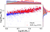 |
Fig. 1. Joint distribution of stellar (M*) and halo masses (M200c) for TNG50-1 central dwarf galaxies at z = 0. All 3297 dwarf galaxies are shown as blue squares, while the 789 dwarf galaxies hosting AGNs are shown as red diamonds. Density histograms represent the marginal distributions of samples in each axis. |
2.5. Control samples
To understand the effect of AGNs, we sought to compare the AGN hosts with non-AGN galaxies. The latter are defined as subhalos where λEdd ≤ 0.1λEdd, min and we used this threshold to ensure that the non-AGN sample is sufficiently different from the AGN sample in terms of black hole accretion rate. All the control samples described below (and represented in Figure 2) are constructed from this sample of non-AGN galaxies (λEdd ≤ 0.001). For clarity, it is relevant to define here the terms used throughout the text. When referring to a dwarf galaxy hosting an AGN, we use the terms “active galaxy” or “AGN host.” Similarly, when we are referring to galaxies that do not host an AGN, we use the terms “inactive galaxy” or “non-AGN galaxy.” The non-AGN galaxies are always part of control samples in our analysis and, thus, they can also be referred to as “control galaxies.” Since many galaxy properties scale with their stellar and halo masses, the non-AGN control samples must have a similar distribution of these variables to isolate the effect of AGN. Motivated by previous works (Ellison et al. 2019) that have demonstrated the importance of considering star formation rate when analyzing AGNs, we also built samples paired by SFR. To evaluate different biases, we created multiple control samples drawn from three different parent samples of non-AGN central galaxies: the set of all non-AGNs (with no restriction, abbreviated as NR), the set of non-AGNs containing gas (WG), and the set of non-AGNs containing black holes (WBH). Galaxies are assigned to these parent samples based on their gas mass (Mgas) and black hole mass (MBH):
-
no restriction (NR): any value of Mgas and MBH;
-
with gas (WG): Mgas > 0 M⊙, any value of MBH;
-
with black holes (WBH): MBH > 0 M⊙, any value of Mgas.
Considering these three sets of non-AGN galaxies, we can independently check if significant differences found in the AGN population still hold if we enforce control galaxies to have gas or black holes. This is important because the simulation can produce dwarf galaxies with no black holes and also dwarf galaxies with no gas reservoir, both of which would be considered non-AGNs by our criteria. On the other hand, by definition, our AGN selection in the simulation will always select dwarf galaxies with Mgas > 0 M⊙ and MBH > 0 M⊙. When comparing the dwarf AGNs with the control galaxies in the NR control samples, we are simply comparing galaxies with and without recent black hole accretion, regardless of their properties. When comparing dwarf AGNs with non-AGN galaxies in the WG control samples, we want to ensure that any differences found will not simply result from control galaxies lacking gas reservoirs. Similarly, when comparing dwarf AGNs with non-AGN galaxies in the WBH control samples, we ensure that any differences found will not simply result from control galaxies lacking a black hole.
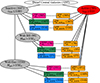 |
Fig. 2. Scheme illustrating the samples referred to in this work. Numbers in parentheses indicate the number of galaxies. From the main sample of dwarf central galaxies in TNG50-1 (white ellipse), we created a sample of AGN hosts (red ellipse). We also created three parent samples of non-AGN galaxies (gray ellipses), one sample of galaxies with no restriction (NR) on their properties, another of galaxies with the restriction of having gas (WG), and another of galaxies with the restriction of having black holes (WBH). Specific non-AGN control samples (pink, green, and blue boxes) are thus drawn from these parent samples, while the corresponding AGN samples (orange boxes) are drawn from the sample of active dwarf galaxies (red ellipse). Dashed lines indicate the pairing of a specific non-AGN control sample and its respective AGN samples, following the method described in Section 2.5. The colors of the boxes of control samples indicate the variables used as control, and correspond to the same colors used in Figure 4. |
To facilitate referencing each specific sample through the text, we adopted the following notation: AGN samples are represented by the letter 𝒮 and non-AGN control samples by the letter 𝒞; subscripts indicate the variables controlled and superscripts represent the parent sample from which galaxies are drawn. For example, the control sample paired by stellar mass and drawn from the parent sample with no restriction (NR) is represented by 𝒞M*NR, while its correspondent AGN sample is represented by 𝒮M*NR. Analogously, the control sample paired by stellar and halo mass, which was drawn from the parent sample of galaxies with gas (WG), is represented by 𝒞M* & M200cWG. To illustrate the structure of the galaxies analyzed here, in Appendix D we present the stellar and mass distributions of a few AGN-control pairs.
To build each control sample, we applied the propensity score matching technique (Rosembaum & Rubin 1983), using the MATCHIT package (Ho et al. 2011). This method allows us to create control samples in which the distributions of the control variables (M*, SFR, M200c) are as similar as possible between AGN and non-AGN samples, with each AGN host paired with a unique inactive galaxy. For the matching parameters, we adopted the Mahalanobis distance (Mahalanobis 2018) approach and the nearest-neighbor method. Additionally, we introduce a final cut ensuring that the maximum difference between individual AGN hosts and their paired control galaxy is 0.1, 0.1, and 0.2 dex in log(M*), log(M200c), and log(SFR), respectively. After the matching process, we perform Anderson-Darling two-sample tests (Anderson & Darling 1952; Scholz & Stephens 1987) to determine whether the properties of control and AGN have similar distributions. This nonparametric statistical test has the null hypothesis that different samples are drawn from the same population, having identical distributions. We chose this specific test in our analysis because it is sensitive to differences in tails of the compared distributions, not only to differences in their central tendencies. When we found a significant difference (up to a significance level of 5%) for a given physical property, we quantify it further through analysis of box plots, and median offsets between AGN and non-AGN samples (see Section 3.2).
Because of the intrinsic distributions of the control variables in TNG50-1 and the adopted criteria for selecting AGNs here, not all dwarf AGN hosts can be paired with a unique non-AGN control galaxy. The direct implication of this is that we can robustly isolate the effect of AGN, with respect to M*, M200c, and SFR, only in a fraction of the dwarf hosts found in the simulation. However, we can guarantee that the effects seen in this subset of dwarf AGNs are due to the recent black hole accretion.
3. Results
3.1. Dwarf AGN fractions
In the stellar mass regime adopted for this work, we found an overall black hole occupation fraction5 of 44% in TNG50-1 at z = 0. When separating the dwarf galaxies by centrals and satellites, we found 53% and 32%, respectively. The overall occupation fraction mentioned above for dwarfs with 8 ≤ log(M*/M⊙)≤9.5 is roughly consistent with some theoretical works (Ricarte & Natarajan 2018; Askar et al. 2022) and observational constraints (Trump et al. 2015; Miller et al. 2015). However, it is worth mentioning that the predictions and constraints for occupation fraction can vary significantly (see the review by Greene et al. 2020). An in-depth comparison of our results with observations requires a careful separation between satellites and central dwarf galaxies in observations, as the satellites in the simulation can have artificially lower fractions. We leave this analysis for future work. For an exhaustive and detailed analysis on the topic of BH occupation fractions in simulations, we refer to the work conducted by Haidar et al. (2022).
Regarding the population of active black holes, after adopting the AGN selection criteria of λEdd ≥ 0.01, we found 1017 AGN hosts from a total of 5909 dwarf galaxies, corresponding to an overall AGN fraction – number of galaxies with active black holes over the total number of galaxies – of 17%. Separating for centrals and satellites, we found 24% and 8%, respectively. The lower AGN fraction on satellite galaxies can be explained mainly by two factors: the absence of bound gas in many satellites and the minimum halo mass for BH seeding. While almost all central galaxies have gas, only half of the satellite dwarf galaxies have a bound gaseous component. Since gas is required for AGN, this prevents many satellite dwarfs from hosting an AGN. Also, due to the black hole seeding model of TNG simulations, if the dwarf galaxy became a satellite before its former host halo reached the minimum halo seeding mass – log(MFoF/M⊙) = 10.868, see Section 2 –, then it will most likely remain without a black hole if it remains a satellite. Thus, a lower occupation fraction is found for the satellite dwarfs, contributing to a lower AGN fraction. For simplicity, in the following analysis and discussions of this work, we focus only on the population of central galaxies.
In Figure 3, we explore how the AGN fraction in central dwarf galaxies changes as a function of the minimum threshold for λEdd and M* in our AGN selection. As the minimum threshold for λEdd increases, the AGN fraction quickly decreases, going from 24% at λEdd, min = 0.01 to 1% at λEdd, min = 0.05 – keeping log (M*,min/M⊙) = 8 constant. The effect of changing the minimum stellar mass is much weaker, since the AGN fraction is mostly constant with respect to M*,min, only changing for more than a few percent at the 9 ≤ log(M*/M⊙)≤9.5 range.
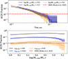 |
Fig. 3. Fraction of central dwarf galaxies hosting AGNs according to different minimum thresholds for variables used in the sample selection. Top panel: AGN fraction as a function of the minimum threshold for λEdd. Bottom panel: AGN fraction as a function of the minimum threshold for stellar mass. In each panel, the solid lines show the fraction for different values of λEdd, min or M*,min, with the shaded regions representing the 95% confidence intervals. The red dashed lines indicate the overall fraction of dwarf AGN candidates from the DESI survey (Pucha et al. 2025), for the whole mass range of 8 ≲ log(M*/M⊙)≤9.5. This value (∼1.2%) is derived from the values presented in their figure 7 (right panel), and is the fraction of dwarf galaxies identified as AGN/Composite in the [N II]–BPT diagram, over the total number of dwarf galaxies (including dwarf galaxies without emission lines). |
A recent work by Pucha et al. (2025) selected dwarf galaxies (log(M*/M⊙)≤9.5) with AGN signatures based on the [N II]–BPT diagram (Baldwin et al. 1981), find an AGN fraction of ∼2.1% among the dwarf galaxies with emission lines. Using the data from their Figure 7 (right panel), we computed the AGN fraction over all dwarf galaxies, regardless of having emission lines, and found a value of ∼1.2% (represented by the red dashed lines in Fig. 3). As it is clear from Fig. 3, the selection of dwarf AGNs in the simulation based simply on λEdd ≥ 0.01 returns a fraction that is more than ten times higher than observations. To reach an AGN fraction comparable to the values from Pucha et al. (2025), the minimum threshold for the Eddington accretion would have to be λEdd, min ≈ 0.05, corresponding to a minimum AGN bolometric luminosity of log(Lbol/ergs s−1) = 43.3 for a host with log(MBH/M⊙) = 6.5 – no obscuration considered. In Section 4.1, we discuss the AGN fractions of TNG50-1 in the broader context of observational works that use different methods for selecting AGNs in real dwarf galaxies.
3.2. Internal properties and environment
Throughout this section, we illustrate the comparison of AGN and non-AGN properties through box plots, assessing the significance of the difference in their distributions with two-sample Anderson-Darling tests. We also use the difference between medians to quantify our statements, noted as Δmed = Med(XAGN)−Med(XControl), where Xsample represents the set of values for a given physical quantity in a given sample. As is shown in the top panel of Figure 4, AGN present higher halo masses when paired only by stellar mass and SFR. This is a direct result of the M* − M200c joint distribution of the dwarf galaxies, as shown in Figure 1, which is a consequence of the halo mass-based seeding model of TNG. This justifies the separate analysis of non-AGN control samples paired by M* and M200c, to guarantee that the differences between AGN and non-AGN are not simply explained by an underlying distinction in their halo mass distributions.
 |
Fig. 4. Box plots of AGN (orange) and non-AGN control (pink, green, blue) sample properties. Each box extends from the first to the third quartile of the data, with a line at the median. The whiskers extend from the box edges to the farthest data point lying within 1.5 times the interquartile range from the box. Data past the end of the whiskers are shown as empty black circles. AGN samples are represented by orange boxes, control samples paired by M*, M* and SFR, or M* and M200c are represented by pink, green, and blue boxes, respectively. Different hatch patterns indicate the different parent samples of non-AGN central galaxies from which the control samples were constructed: no pattern, “x” pattern, and dot pattern refer to the “no restriction” (NR), “with gas” (WG), and “with BH”‘ (WBH) samples, respectively. The legend above the upper panel indicates the color and hatch pattern for each control sample shown in the figure. In each panel, above the boxes, we show the number of AGN hosts (NAGN), the difference between the median of the AGN and control (Δmed), and the p-value of an Anderson-Darling two-sample test performed with the control+AGN paired samples. In the cases where the difference was considered statistically significant (p-value < 0.05), the upper text is highlighted as bold and enclosed in a red box. From top to bottom, the panels show box plots for host halo mass, neutral-to-total gas ratio, and gas half-mass radius. |
The most substantial differences that we found for dwarf AGN properties were in their gas component. In the lower panels of Figure 4, we show the ratio of neutral-to-total gas mass ratio (Mneutral/Mgas) and the gas half-mass radius (Re, gas). It is evident that dwarf AGNs are significantly different from their control in these properties, regardless of the adopted parent sample or control variables, although the differences are less pronounced in control samples with BH. The vast majority of control galaxies have Mneutral/Mgas above 0.25, while the majority of AGNs have Mneutral/Mgas < 0.2. Additionally, for almost all control samples, Δmed of Mneutral/Mgas is close to 0.2, meaning that the dwarf AGN population has approximately 20% less of its gas in the neutral form when compared to the non-AGN sample. If we also compare the extension of the gas radius in AGNs and non-AGNs, especially for 𝒞M* & M200cWG, we find that Re, gas in AGNs is usually more than 10 kpc larger, with the majority of AGNs having Re, gas > 25 kpc. Although some differences in Mneutral/Mgas are systematically more minor for 𝒞M*WBH, 𝒞M* & SFRWBH and 𝒞M* & M200cWBH control samples, they are still not negligible, implying that just the presence of black hole is not enough to explain the distinct gas properties in dwarf AGN. As discussed in Section 3.4, the deficiency in neutral gas is not only connected with the black hole presence in these dwarf galaxies, but also to their recent activity in the radiative mode.
We also analyzed other relevant properties of AGN hosts measured inside 2Re, *, like their metallicity (Z*), age (t50), and specific SFR (sSFR), shown in Figure 5. No significant large differences are found when controlling for halo and stellar mass, except for sSFR. AGN hosts tend to be less star-forming, with the median sSFR of control galaxies being 1.4 times larger than the median sSFR of AGN. Interestingly, observations of AGNs in more massive hosts suggest opposite results (Mountrichas et al. 2024; Riffel et al. 2024). This difference in log(sSFR) is similar (Δmed ≈ 0.1 dex) for other non-AGN control samples where SFR is not controlled, and may be an indirect effect of the AGN hosts having less neutral gas available. In observational studies, it may be challenging to obtain the halo mass of dwarf galaxies, with non-AGN control samples only being able to be paired by stellar mass. When only M* is controlled in our analysis, in addition to having lower sSFR, AGN hosts also have lower stellar metallicities and lower t50. Although statistically significant, the magnitude of these differences is small, as evidenced by the box plots and comparison of the medians in the figure.
 |
Fig. 5. Same as Figure 4, but (from top to bottom), the box plots show the specific star formation rate, stellar metallicity, median stellar formation time, and distance to the first-nearest neighbor (with M* ≥ 108 M⊙). |
Furthermore, we analyzed the distances to nearest neighbors of the galaxies (Figure 5) to explore possible relations between the environment and AGN activity. This analysis is also important to reinforce the results found for the neutral gas, excluding the possibility of AGNs having different neutral gas fractions simply due to perturbations in their immediate vicinity. As shown in the lower panel of Figure 5, for the 1st nearest neighbors (d1, M8), most control samples show no significant difference in their distribution when compared to AGN samples, and those that have statistically significant differences (e.g., the sample 𝒞M*NR), have it very slightly. For example, the sample 𝒞M*WBH shows the largest Δmed for log(d1, M8/kpc), however this difference (0.17 dex) yet large in terms of physical size (∼300 kpc), is not physically relevant due to the typical values of d1, M8. The distances to the first neighbors are larger than 300 kpc for 90% of the galaxies, implying that the gravitational pull from the closest companions is already weak, and the difference found in the median of d1, M8 should not be relevant for the AGN activity. Thus, since the difference in the distributions of distance to neighbors is even smaller for other control samples, it is unlikely that the presence of immediate neighbors at d > 300 kpc significantly impacts black hole activity of the simulated dwarf galaxies. The results remains the same if we consider other metrics to measure environment, such as the distance to the first massive nearest neighbor (d1, M10) or distance to the farthest neighbors (d10, M8 and d10, M10), which probe the environment in slightly larger scales (see Appendix C). In line with the result described above, observational works measuring the small-scale environment of AGN hosts also found that they have similar environments compared to non-AGN control galaxies matched in redshift, stellar mass, and morphology (Rembold et al. 2024). A previous work by Kristensen et al. (2021) analyzes the TNG100-1 simulation run and finds evidence of a non-negligible role of environment for AGN activity in dwarf galaxies with 9 ≤ log(M*/M⊙) < 9.48. We do not find the same trends when analyzing central dwarf galaxies in this work. The difference between the results may come from the absence of satellite galaxies in our analysis, the different stellar mass distribution of the AGN samples, and the difference in simulation volume or resolution.
As described above, the strongest differences between AGNs and non-AGNs are in the gas half-mass radius and neutral gas content. However, the differences between 𝒞M*WBH and 𝒮M*WBH present a different behavior than other non-AGN and AGN paired samples. Although AGN hosts in 𝒮M*WBH are still more deficient than their control counterparts, 𝒞M*WBH shows more pronounced tails towards zero on the distributions of Mneutral/Mgas. When compared to other control samples, 𝒞M*WBH also shows more pronounced tails towards lower values of sSFR and t50. When compared to its AGN counterpart, 𝒞M*WBH contains relatively older and more quiescent galaxies, indicating that if we impose the restriction of having a BH and only control for stellar mass, we may find that active dwarf galaxies formed more recently than inactive ones. The distributions of d10, M8, d10, M10 and d1, M10 for 𝒞M*WBH also present more pronounced tail towards smaller distances, suggesting slightly denser environments than their paired AGN. However, the difference in environment does not seem to be important given the absolute values of the distances to neighbors (≳300 kpc).
3.3. Differences in the gas component at z = 0
In this section, we focus on the comparison of the specific AGN sample 𝒮M* & M200cWG with its respective control sample 𝒞M* & M200cWG. The goal of focusing on this comparison is to ensure that differences in the neutral gas content are not consequences of a stellar or a halo mass bias, and also guarantee that all galaxies being compared have a gaseous component. We first analyze the difference in the gas radial profiles, more specifically, volumetric density (ρgas), neutral-to-total mass ratio, and temperature profiles (Figure 6).
 |
Fig. 6. Spherical gas profiles of AGN (orange) and non-AGN control (blue) samples. From top to bottom, we show the radial profiles of the volumetric gas density, the neutral-to-total gas mass ratio, and the gas temperature. In both panels, the thin semitransparent lines represent the profiles of individual galaxies, the thick solid lines represent the median profile of the whole sample, and the dashed lines indicate the 16th and 84th percentiles. The radial distance to the galaxy center (r) is rescaled by Re, *. The difference between median AGN and non-AGN profiles for a given quantity (Δ) is shown in black on the lower small sub-panels. The samples being compared here are 𝒮M* & M200cWG and 𝒞M* & M200cWG. |
From the comparison of density profiles, we see that AGNs have slightly less dense gas from ∼2Re, * to ∼20Re, *; however, the difference between the median profiles is well within the scatter of both samples. On the other hand, it is evident from the direct comparison of AGN and non-AGN median profiles that the neutral gas deficiency is strong already at the inner parts of the gas component (≲2Re, *), even considering the scatter of the profiles in each sample. The smaller values of Mneutral/Mgas for the dwarf AGNs are more significant in the ∼2Re, * to ∼8Re, * radial interval, where the scatter of AGN and non-AGN profiles do not even overlap. Nonetheless, we can see that the AGN sample has relatively less neutral gas from ∼1Re, * to ∼15Re, *. The temperature of the gas is related to the neutral hydrogen fraction in each gas cell (i.e., hotter cells will usually have less neutral hydrogen), but although we see clear differences in the neutral content for the inner part of the gas component, the same is not true for the gas temperature. The AGNs have hotter gas in their outskirts (r ≳ 10Re, *) and mostly similar temperatures for the gas within ∼5Re, *, where gas cooling is stronger.
In the upper panel of Figure 7, we show the neutral gas masses in AGNs and non-AGNs at different apertures. It is clear that the total amount of neutral gas in the control galaxies is higher, with AGN hosts having, on average, 3.9 times less mass in this component than their matched non-AGN counterparts (from the 𝒞M★ & M200cWG sample). When only the stellar mass is controlled, in an approach that is similar to what is commonly done in observational works (Rembold et al. 2024; Albán et al. 2024; Gatto et al. 2025), we found that the AGN hosts still have, on average, 2.5 times less neutral gas than non-AGN hosts (see Appendix A). To illustrate that the difference in Mneutral is stronger in the circumgalactic medium6 (CGM), we also show histograms of the masses within two stellar half-mass radii. As shown in the figure, the neutral gas mass confined to the inner parts of the galaxies is very similar between AGN and non-AGN samples. This result emphasizes that the strongest imprint the black hole accretion is leaving on dwarf galaxies is in the outskirts of their gaseous halo.
 |
Fig. 7. Histograms of neutral, neutral atomic (H I), and molecular (H2) gas masses for the AGN (orange) and non-AGN control (blue) samples. The upper panel shows the bound neutral gas masses, with the solid line indicating the total amount and the dashed line indicating only the mass within 2Re, *. The middle and lower panels show the total bound gas masses in the form of H I and H2, taken from the TNG supplementary catalog (Diemer et al. 2019). Each line style of the histograms refers to a type of partition model considered by Diemer et al. (2019) in their post-processing: solid lines are from Gnedin & Draine (2014), dashed lines are from Gnedin & Draine (2014), dotted lines are from Krumholz (2013), and dotted-dashed lines are from Sternberg et al. (2014). Here, we show different models to illustrate variations in the values of MH I and MH2. In the upper right of each panel, we show the average pair-wise differences (Δpair) between the AGN and non-AGN logarithmic masses. The samples being compared here are 𝒮M* & M200cWG and 𝒞M* & M200cWG. |
Using the supplementary catalog from Diemer et al. (2019), we also analyze the difference in the individual phases of the neutral gas, that is, we study the mass distributions of H I and molecular gas. As shown in the middle and lower panels of Fig. 7, the deficit of neutral gas is also reflected in a deficit of H I and molecular gas for the AGN, regardless of the partition model adopted. For the neutral atomic component, there is little variation on the distributions of mass with respect to models, and we find that MH I is, on average, 4.8 times lower in AGNs when stellar and halo mass is matched in the control sample (𝒞M* & M200cWG), or 3 times lower when only stellar mass is matched (𝒞M*WG, see Appendix A). For the molecular component, the values of MH2 show a stronger dependence on the adopted model, and on average, MH2 is 2.1 times lower in the AGNs relative to 𝒞M* & M200cWG, and 1.6 times lower relative to 𝒞M*WG. There are a number of modeling choices underlying the values of MH I and MH2 shown in Figure 7, and the exploration of specific effects from each model is beyond the scope of this work, we refer to the works of Diemer et al. (2018) and Diemer et al. (2019) for that. Nonetheless, the current results show that AGN presence in simulated dwarf galaxies of TNG50-1 is possibly associated with a decrease in their total H I and molecular gas masses.
It is also important to note which of the two AGN feedback modes employed in TNG impacts the most. Active dwarf galaxies are selected here to have λEdd ≥ 0.01, and the transition for the low-accretion kinetic mode only happens if λEdd < χ, where χ = min[0.002 × (MBH/108 M⊙)2, 0.1] is a mass-dependent threshold (Weinberger et al. 2017). Since χ ≲ 0.002 for the dwarf galaxies hosting an AGN at z = 0, it is the high-accretion thermal feedback that dominates the liberated feedback energy.
3.4. Evolution of gas properties
In the previous sections, we showed that the AGN hosts at z = 0 have less neutral gas than non-AGN galaxies with similar stellar and halo masses. Since we can follow the complete history of individual galaxies in a simulation, we can explore the causal effects of black hole accretion on the gas phase of the simulated dwarf galaxies. As in the last section, here we focus on the 𝒮M* & M200cWG AGN sample and its 𝒞M* & M200cWG control sample for comparisons.
In Figure 8, we show the evolution of different properties of AGN and non-AGN control samples. It is clear from the evolution of the Mneutral/Mgas that the AGN hosts suffer a sudden decline in their neutral content after the seeding of the black holes, which are actively accreting as soon as they are seeded7. The evolution of the gas temperature also reflects this effect since the AGNs also have higher temperatures compared to the control galaxies at t > tseed. The AGNs essentially stay in the high-accretion regime during their entire evolution. Thus, the direct effect of an AGN is the injection of thermal energy into the gas near the black hole (Weinberger et al. 2017). It could be argued that the decrease in the neutral gas content is related to an increase in the SFR of the galaxies, which in turn would cause more intense stellar feedback. However, as is shown in the bottom left panel of Figure 8, non-AGNs and AGNs have similar SFR before tseed, making it unlikely that star formation processes are solely responsible for the decrease in Mneutral. Indeed, the median SFR of the AGN hosts immediately after tseed is even slightly lower, although the difference is within the scatter of both samples. Furthermore, there is no strong difference in the evolution of the total gas mass or the halo mass, excluding the possibility of the decrease in the neutral gas fraction being a consequence of different halo assembly histories in AGN and non-AGN samples.
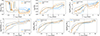 |
Fig. 8. Evolution of properties in AGN (orange) and non-AGN control (blue) samples. The time variable on the horizontal axis is the cosmic time minus the seeding time (tseed) of the AGN host. where the median tseed is 11 Gyr, and the 16th (84th) percentile is 7.3 Gyr (13 Gyr). From top to bottom and left to right, each panel represents the evolution of the neutral-to-total gas ratio, gas temperature, neutral gas mass, star formation rate, total gas mass, and host halo mass. All bound gas particles are considered. The solid lines indicate the median evolution of a given quantity for the whole sample, while the dashed lines indicate the 16th and 84th percentiles. Different from Figure 6, here we choose not to plot the data of each galaxy for better visualization. The samples being compared here are 𝒮M* & M200cWG and 𝒞M* & M200cWG. |
On average, for 𝒞M* & M200cWG, the difference in neutral gas mass is set in place quickly after tseed, being present for several Gyr after. However, by analyzing galaxies in 𝒞M* & M200cWBH – control sample with restriction of having a black hole (see Appendix A) – we found a different picture. The difference in neutral gas does not appear immediately after black hole seeding, but ∼4 Gyr later, when the accretion rates in control galaxies start to decrease (see Figure A.5). Thus, the neutral gas deficiency in dwarf AGNs is not only directly linked to the black hole seeding, but also to its black hole matter accretion history in the last few Gyr.
We can also see the direct effect of AGN feedback in the neutral-to-total gas profiles of individual galaxies, as illustrated with a few examples in Figure 9. We show the profiles at three different times, for randomly selected AGN hosts with different stellar masses and different tseed. In general, all the Mneutral/Mgas profiles suffer a strong decrease in their values after the AGN starts, with the most noticeable difference appearing on the galaxies with recent BH seeding (tseed < 1 Gyr), regardless of stellar mass. Due to the limited size of the sample, a binning of the galaxies in the space of M* and tseed results in only a few galaxies per bin, hindering a robust statistical analysis. Thus, we restrict our analysis of the effect of these variables on the profiles to a qualitative presentation of illustrative random examples. Since the impact of AGNs on Mneutral/Mgas profiles is more evident on the hosts with more recent tseed, it is possible that the AGN does not permanently decrease the neutral gas content on dwarf galaxies.
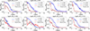 |
Fig. 9. Examples of neutral-to-total gas profile evolution for a few AGNs selected at z = 0. In each panel, we show the profile of a specific galaxy at different times, before and after the black hole seeding. The two latest available profiles before tseed are shown as blue and gray solid lines, the earliest available profile after tseed is shown as a red solid line, and the present profile is shown as a black dotted line. The availability of the profiles depends on the type of simulation snapshot; see Section 2.3 for details. Each row is dedicated to a bin of black hole seeding times, in the top row tseed < 1 Gyr, and in the bottom row tseed > 3 Gyr. From left to right: Stellar mass of the example galaxies increasing in bins of roughly 0.25 dex. |
4. Discussion
4.1. Dwarf AGN demographics
The demographics of AGNs in dwarf galaxies are essential for understanding galaxy evolution (Mezcua & Domínguez Sánchez 2020; Arjona-Gálvez et al. 2024) and may inform studies on massive black hole formation (Greene et al. 2020; Reines 2022). Thus, checking the BH occupation and AGN fractions on state-of-the-art cosmological simulations is important. In observations, the selection of dwarf AGNs is challenging, and the determination of the AGN fraction is subject to several biases (Hainline et al. 2016; Agostino & Salim 2019; Latimer et al. 2021b; Sturm et al. 2025), which can result in significant variations of reported fractions (Haidar et al. 2022). For example, sources identified by X-rays and infrared diagnostics are often not classified as AGNs through optical spectroscopy (Wasleske & Baldassare 2024). This lack of overlap in the samples selected by different techniques can be partly explained by a few factors, such as dilution of the AGN signatures within star formation (Moran et al. 2002; Trump et al. 2015), varying ionizing spectrum with decreasing BH mass (Cann et al. 2019), off-nuclear emission (Thygesen et al. 2023), and changes in the emission line ratios due to low metallicities (Groves et al. 2006).
As shown in Section 3.1, our analysis of the small volume of TNG50 yields an overall BH occupation fraction on dwarf galaxies of 44%, which is broadly consistent with observational constraints for log(M*/M⊙)≤9.5 (Miller et al. 2015; Greene et al. 2020; Cho & Woo 2024). Furthermore, we found AGN fractions that span more than one order of magnitude - ∼1% (λEdd, min = 0.05) to ∼24% (λEdd, min = 0.01) - depending on the minimum accretion rate adopted for the AGN selection. In contrast, different observational estimates, based on X-ray (Schramm & Silverman 2013; Lemons et al. 2015; Miller et al. 2015; Mezcua et al. 2018; Birchall et al. 2020) and optical (Reines et al. 2013; Sartori et al. 2015; Cho & Woo 2024) selection methods, found AGN fractions tend to be below 2% for galaxies with log(M*/M⊙)≤9.5. Only a few exceptions in the literature report fractions of the same order of magnitude as we find in TNG50. For example, Kaviraj et al. (2019) selected AGNs in dwarf galaxies at 0.1 ≤ z ≤ 0.3 using WISE infrared photometry, and found the AGN fraction to be in the range of 10% to 30% for 8 ≤ log(M*/M⊙)≤9.5. A more recent work, by Mezcua & Domínguez Sánchez (2024) analyzed data from MaNGA DR17 and selected AGNs using a combination of [N II]–BPT, [S II]–BPT and [O I]–BPT diagrams and the WHAN diagram (Cid Fernandes et al. 2010). Their initial estimate for AGN fraction in MaNGA was of ∼20%, but after a correction in the stellar masses and SFRs used in their paper (Mezcua & Domínguez Sánchez 2025), considering only galaxies with log(M*/M⊙)≤9.5 in their sample, the updated fraction8 falls to ∼14%. On the other hand, a more recent work by Pucha et al. (2025) presented an analysis of DESI survey, also selecting AGNs using BPT diagrams and finding an AGN fraction of ∼1.2% (computed from their Figure 7) over all dwarfs with log(M*/M⊙)≤9.5. For a comprehensive list of AGN fractions estimated for galaxies with log(M*/M⊙)≤10 at low redshift, we refer to Appendix A of Haidar et al. (2022), which exhaustively lists the reported AGN fractions in the literature.
Except for a few works, most of the AGN fraction estimates in the literature are at least one order of magnitude below the value of 24% that we found in our fiducial selection sample here (λEdd, min = 0.01). This discrepancy between the simulation and observations may arise from a heavy BH seed implemented in TNG (Habouzit et al. 2021; Haidar et al. 2022), but also from an intrinsic difficulty in detecting all active black holes in observed dwarf galaxies, as discussed above. Nonetheless, it is important to be careful when comparing AGN fractions from studies that use different AGN detection techniques, since they can trace different AGN populations (Riffel et al. 2023; Wasleske & Baldassare 2024; Albán et al. 2024; Tian et al. 2025), and also possibly introduce their own specific biases on the estimates of AGN fraction in dwarfs.
As we show in the top panel of Figure 10, the bulk of the dwarf AGNs identified in TNG50 have bolometric luminosities (Lbol) mostly between 1042.5 and 1043.5 erg s−1, with X-ray luminosities mostly in the range of 1041.5–1042.5 erg s−1. It has been argued that the X-ray detection of AGNs in dwarf galaxies could be contaminated by X-ray binaries (Mezcua et al. 2018; Thygesen et al. 2023); thus, it is valid to compare the luminosities of both types of sources to understand which dominates the X-ray emission. We can also see in the lower panel of Figure 10 that XRB luminosities are expected to be more than 100 times fainter than AGN luminosities. Similarly, Schirra et al. (2021) analyzed TNG100 and found that the AGNs usually dominate the X-ray luminosity for log(M*/M⊙) < 10.5. Thus, according to this simple estimate, AGNs should dominate the X-ray luminosities in active dwarf galaxies with similar M* and Lbol as those studied here.
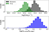 |
Fig. 10. Top: histogram of AGN luminosities, bolometric (black), and total (0.5–10 keV) X-ray (green). Bottom: histogram of the ratio between AGN and X-ray binaries (XRB) luminosities. No extinction or obscuration is considered (see Section 2 for details on calculation). |
In our analysis, the minimum stellar mass chosen for the selection of dwarf AGN galaxies does not strongly affect the AGN fraction, at least in the 8 ≲ log(M*/M⊙)≲9 mass interval. However, as we increase the minimum threshold for the Eddington ratio, the AGN fraction rapidly decreases, and since previous works found a relation between BH accretion rate and H I gas (Li et al. 2025), it is relevant to verify if our results change with λEdd. As shown in Figure 3, the AGN fraction is most similar to observational estimates only when λEdd, min ≳ 0.05. If we consider AGN-only dwarf hosts with λEdd ≥ 0.05, the results for neutral gas deficiency remain the same (see Appendix B).
4.2. Neutral gas deficiency
As shown by the evolution of the global gas properties and the evolution of individual profiles, the decrease in the neutral gas mass is a direct effect of AGN feedback on dwarf galaxies. The reduction of the neutral component is not only caused by the initial triggering of the feedback but is also maintained by the cumulative effect of multiple accretion peaks over a few billion years. Previous theoretical works also find that the cumulative energy injected by the AGN onto the gas can decrease the atomic-to-stellar mass ratio (Weinberger et al. 2017; Ma et al. 2022; Li et al. 2025). While it has been demonstrated that the kinetic feedback mode holds an important role in the quenching of more massive simulated galaxies (Weinberger et al. 2017; Terrazas et al. 2020), this type of feedback is not present in the dwarf AGNs analyzed here. The black hole feedback in action is the high-accretion thermal feedback mode employed in the IllustrisTNG model. Similar results were found by Li et al. (2025), where the authors analyzed larger (but at a lower resolution) simulations (TNG100 and EAGLE) and found that H I gas is regulated mainly by thermal-mode AGN feedback in TNG. Sharma et al. (2020) also finds lower H I content in isolated dwarf galaxies (9 ≤ log(M*/M⊙)≤10), with over-massive black holes in the ROMULUS25 simulation. Furthermore, using the AURIGA galaxy formation physics model, Arjona-Gálvez et al. (2024) compared simulation runs with and without AGN feedback in dwarf galaxies. They found that the feedback in these systems leads to a decrease in the amount of H I gas. However, the reduction in H I is not due to the gas being expelled from the galaxy, but rather due to heating of the gas in the vicinity of the AGN, which lowers the fraction of gas in the cold, neutral phase. However, Koudmani et al. (2022) finds different results regarding the gas content in dwarf AGN. They performed a large suite of zoom-in simulations varying seeding times, seeding masses, and the length of the AGN duty cycle, and founds that the H I gas masses of dwarfs are either completely suppressed or within the scatter of the observed MH I − M* relations for field dwarfs.
In the observational domain, different results are reported on the H I content of AGN hosts. While some studies found that AGN hosts and inactive galaxies have similar MH I/M* for log(M*/M⊙)≥10 (Fabello et al. 2011), others found that AGNs can be even more gas-rich than their non-AGN counterparts (Ho et al. 2008). Furthermore, a few works predict mixed results for the stellar mass range of 9 ≤ log(M*/M⊙)≲10 (Bradford et al. 2018; Ellison et al. 2019). Bradford et al. (2018) investigated the global H I content of isolated galaxies selected from the SDSS spectroscopic survey with optical evidence of AGN activity, identifying a set of galaxies at large distances from the BPT star-forming sequence having lower than expected H I masses. The galaxies in which this H I gas deficit was found are in the stellar mass range of 9.2 < log(M*/M⊙) < 9.5. In another work, Ellison et al. (2019) investigated the H I gas fractions of AGN hosts in the extended GALEX Arecibo SDSS Survey (xGASS), finding that at fixed stellar mass, AGN hosts with 9 < log(M*/M⊙) < 9.6 show an H I deficit that reaches a factor of ∼2 when the control sample is matched by stellar mass and SFR.
To investigate the trend of H I gas deficiency as a function of stellar mass, we selected all central galaxies in TNG50-1 containing neutral gas and computed MH I/M* in logarithmic stellar mass bins of 0.5 dex from log(M*/M⊙) = 8 to log(M*/M⊙) = 11.5. We then created a sample of AGNs (λEdd ≥ 0.01) and a control sample of non-AGNs matched only by stellar mass9, similar to what is commonly done in other observational works (Rembold et al. 2024; Albán et al. 2024; Gatto et al. 2025). The comparison of the atomic-to-stellar mass ratio of AGNs versus non-AGNs is shown in Figure 11 – with MH I being the average of the four volumetric estimates from Diemer et al. (2019). We find a qualitatively similar trend as the observational results from Ellison et al. (2019), that is, the deficiency of H I gas in AGN hosts becomes stronger for lower stellar masses, reaching the maximum difference in MH I/M* at the minimum M* considered here.
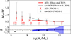 |
Fig. 11. Median atomic-to-stellar mass ratio (MH I/M*) for AGNs (red stars) and non-AGNs (gray circles) in different stellar mass bins (upper panel) of TNG50-1. Error bars mark the 16th and 84th percentiles for each bin. The small lower panel indicates the difference between the medians of the AGN (λEdd ≥ 0.01) and non-AGN samples. The position of the markers on the x-axis corresponds to the median stellar mass of the galaxies in the bin. The number of objects in each mass bin is indicated by their corresponding colors. The samples of AGNs and non-AGNs are paired by stellar mass and contain only central galaxies. We also plot the MH I/M* values (red and gray solid lines) and uncertainties (shaded regions) reported on Ellison et al. (2019) (their Figure 8), which compares AGNs and non-AGNs in fixed stellar-mass bins. In the bottom panel, we show as a blue line the corresponding AGN-to-non-AGN difference from Ellison et al. (2019). |
Our findings could be further tested through a detailed comparison with radio observations. For example, one could combine catalogs of dwarf AGN candidates from SDSS and DESI (Reines et al. 2013; Pucha et al. 2025) with the single-dish mass estimates from the Arecibo Legacy Fast ALFA (ALFALFA) survey (Haynes et al. 2018) or the more recent FAST All Sky H I Survey (FASHI) (Zhang et al. 2024), both with large coverage of the north sky. More than 80% of the dwarf AGNs selected in this work have log (MH I/M⊙ > 8, which are measurable up to z ≈ 0.015 combining ALFALFA and FASHI catalogs, or z ≈ 0.01 assuming only half of the total H I mass is detected. However, for a robust comparison, with a large sample (number of objects > 500) of dwarf AGN candidates, deeper radio observations would be needed to cover redshifts up to z = 0.05.
Regarding molecular gas, studies on local luminous AGNs have found that they are characterized by similar molecular gas fractions to inactive galaxies with similar infrared luminosity (proxy to stellar mass) (Rosario et al. 2018), similar sSFR (Saintonge et al. 2017), or compared to normal star-forming disc-dominated galaxies (Husemann et al. 2017). However, these works address the molecular gas content of AGNs in hosts mostly with log(M*/M⊙)≳9.5, and a similar analysis focusing on a sample of confirmed dwarf AGNs would be useful for testing our results.
As shown in the examples of Figure D.1 and in our results in Section 3.2, the dwarf galaxies hosting AGNs can have similar stellar structures and similar stellar properties as other non-AGN galaxies of comparable stellar and halo masses. However, the distribution and global properties of their CGM can be radically different, especially in terms of the gas thermodynamic properties. A hotter gas reservoir, with less neutral gas available, may entail a decline of future star formation on the central dwarf galaxies that suffered from the black hole feedback. Furthermore, given the frailty of the CGM of dwarf galaxies during interaction with more massive galaxies (Pearson et al. 2016; Zhu et al. 2024), the AGN feedback could aggravate the situation, facilitating further gas removal in case they become satellites in groups or clusters. In this sense, the analysis of the CGM in the low-mass regime may be a powerful approach to understanding the baryon cycle of dwarf galaxies (Piacitelli et al. 2025) and also to test the predictions of cosmological simulations employing completely different subgrid physics (Zinger et al. 2020; Liu et al. 2025; Medlock et al. 2025). Thus, our results contribute to ongoing efforts by providing useful insights into the interaction between AGNs and the gaseous component of central dwarf galaxies, especially in light of upcoming surveys from new facilities (e.g., Vera C. Rubin Observatory, Square Kilometer Array), which will expand our view of galaxies down to lower masses.
5. Conclusions
In this work, we searched for dwarf galaxies hosting AGNs in the TNG50-1 cosmological simulation and investigated their demographics. We also studied the effects of AGN feedback by comparing these active dwarf galaxies with inactive ones using multiple control samples, paired with the stellar and halo mass. Based on our analysis of central dwarf galaxies (8 ≤ log M*/M⊙ ≤ 9.5) at z = 0, we can summarize our conclusions as follows:
-
The fraction of dwarf galaxies hosting AGNs at z = 0 varies from 1% (λEdd, min = 0.05) to 24% (λEdd, min = 0.01), depending on the adopted threshold for Eddington ratio (Figure 3). The simulation may overestimate the fraction of active BHs in dwarf galaxies compared to observations, although different Eddington ratio cuts and AGN detection methods can yield varying reported fractions.
-
AGN hosts are deficient in neutral gas when compared to non-AGN hosts of similar stellar mass, SFR, and halo mass. They also have more extended gas halos, having gas radii that are at least ∼10 kpc larger (Figure 4).
-
The sample of AGN hosts have log(sSFR) lower by ≳0.1 dex gh compared to non-AGNs of similar stellar and halo mass. On the other hand, we found no differences in terms of stellar metallicity and age (Figure 5).
-
We also found no distinguishable difference in the environment of dwarf AGN hosts and control galaxies as measured by the distance to their neighbors (Figure 5).
-
The neutral gas deficiency in AGN hosts is stronger beyond two stellar half-mass radii (2Re, * ≈ 2.8 kpc, typically). The onset of this dearth in neutral gas in the CGM of dwarf galaxies is caused by the BH thermal feedback (Figures 6 and 8).
-
The neutral gas component in the AGN sample is, on average, ∼3.9 times less massive than in the non-AGN control sample (matched by stellar and halo mass). Similarly, the H I mass in AGN hosts is ∼4.8 times lower (Figure 7). If only stellar mass is matched, dwarf AGNs still have, on average, ∼2.5 times less neutral mass and ∼3 times less H I mass.
-
The MH I/M* fraction of dwarf AGNs and non-AGNs becomes increasingly different towards lower stellar masses, with most dwarf AGNs characterized by MH I/M* < 2 for log(M*/M⊙) < 10 (Figure 11).
The high AGN fraction found in this work relative to observations at log(M*/M⊙)≤9.5 highlights the importance of precise black hole seeding models in cosmological simulations, especially for the low-mass regime. Additionally, it motivates a future detailed investigation on AGN selection methods and how each method relates to different cuts in the Eddington ratio. On the other hand, the prediction of lower neutral gas fractions in the gas reservoirs of dwarf galaxies is qualitatively consistent with observational results (Ellison et al. 2019). This is especially important because it represents a direct imprint of the subgrid models employed in IllustrisTNG. Further testing this prediction with future observational works can be valuable with respect to the development of more accurate and effective models in future cosmological simulations. Current and future observational facilities (e.g., JWST, Vera C. Rubin Observatory, SKA, ATHENA) will likely provide a rich and large amount of data on dwarf galaxies across different wavelengths, enabling the study of these galaxies with unprecedented detail. Finally, investigating AGN activity in dwarf galaxies is important for understanding the exact impact of black holes on the low-mass end of the galaxy stellar mass function.
Acknowledgments
The authors thank the referee for the comments that led to an improved version of the manuscript. RFF thanks the support of Conselho Nacional de Desenvolvimento Científico e Tecnológico (CNPq) and the support from Coordenação de Aperfeiçoamento de Pessoal de Nível Superior (CAPES). MT thanks the support of CNPq (process #312541/2021-0). RAR acknowledges the support from CNPq (Proj. 303450/2022-3, 403398/2023-1, & 441722/2023-7) and CAPES (Proj. 88887.894973/2023-00). RR acknowledges support from CNPq (Proj. CNPq-445231/2024-6,311223/2020-6, 404238/2021-1, and 310413/2025-7), Fundação de amparo à pesquisa do Rio Grande do Sul (FAPERGS, Proj. 19/1750-2 and 24/2551-0001282-6) and CAPES (88881.109987/2025-01). BDO acknowledges the support from the CAPES (88887.985730/2024-00). This work was conducted during a scholarship supported by the International Cooperation Program PROBRAL at the Ruprecht Karl University of Heidelberg. Financed by CAPES – Brazilian Federal Agency for Support and Evaluation of Graduate Education within the Ministry of Education of Brazil. The IllustrisTNG simulations were undertaken with compute time awarded by the Gauss Centre for Supercomputing (GCS) under GCS Large-Scale Projects GCS-ILLU and GCS-DWAR on the GCS share of the supercomputer Hazel Hen at the High Performance Computing Center Stuttgart, as well as on the machines of the Max Planck Computing and Data Facility in Garching, Germany.
References
- Agostino, C. J., & Salim, S. 2019, ApJ, 876, 12 [NASA ADS] [CrossRef] [Google Scholar]
- Albán, M., Wylezalek, D., Comerford, J. M., Greene, J. E., & Riffel, R. A. 2024, A&A, 691, A124 [NASA ADS] [CrossRef] [EDP Sciences] [Google Scholar]
- Anderson, T. W., & Darling, D. A. 1952, Ann. Math. Stat., 193 [Google Scholar]
- Aravindan, A., Canalizo, G., Secrest, N., Satyapal, S., & Bohn, T. 2024, ApJ, 975, 60 [Google Scholar]
- Arjona-Gálvez, E., Di Cintio, A., & Grand, R. J. J. 2024, A&A, 690, A286 [NASA ADS] [CrossRef] [EDP Sciences] [Google Scholar]
- Askar, A., Davies, M. B., & Church, R. P. 2022, MNRAS, 511, 2631 [NASA ADS] [CrossRef] [Google Scholar]
- Baldwin, J. A., Phillips, M. M., & Terlevich, R. 1981, PASP, 93, 5 [Google Scholar]
- Bellovary, J. M., Cleary, C. E., Munshi, F., et al. 2019, MNRAS, 482, 2913 [NASA ADS] [Google Scholar]
- Birchall, K. L., Watson, M. G., & Aird, J. 2020, MNRAS, 492, 2268 [NASA ADS] [CrossRef] [Google Scholar]
- Bondi, H. 1952, MNRAS, 112, 195 [Google Scholar]
- Bondi, H., & Hoyle, F. 1944, MNRAS, 104, 273 [Google Scholar]
- Bower, R. G., Benson, A. J., Malbon, R., et al. 2006, MNRAS, 370, 645 [Google Scholar]
- Bradford, J. D., Geha, M. C., Greene, J. E., Reines, A. E., & Dickey, C. M. 2018, ApJ, 861, 50 [NASA ADS] [CrossRef] [Google Scholar]
- Cann, J. M., Satyapal, S., Abel, N. P., et al. 2019, ApJ, 870, L2 [NASA ADS] [CrossRef] [Google Scholar]
- Cattaneo, A., Faber, S. M., Binney, J., et al. 2009, Nature, 460, 213 [NASA ADS] [CrossRef] [Google Scholar]
- Cho, H., & Woo, J.-H. 2024, ApJ, 969, 93 [Google Scholar]
- Cid Fernandes, R., Stasińska, G., Schlickmann, M. S., et al. 2010, MNRAS, 403, 1036 [Google Scholar]
- Dashyan, G., Silk, J., Mamon, G. A., Dubois, Y., & Hartwig, T. 2018, MNRAS, 473, 5698 [CrossRef] [Google Scholar]
- Davidzon, I., Ilbert, O., Laigle, C., et al. 2017, A&A, 605, A70 [NASA ADS] [CrossRef] [EDP Sciences] [Google Scholar]
- Davis, F., Kaviraj, S., Hardcastle, M. J., et al. 2022, MNRAS, 511, 4109 [NASA ADS] [CrossRef] [Google Scholar]
- De Lucia, G., & Blaizot, J. 2007, MNRAS, 375, 2 [Google Scholar]
- Dekel, A., & Silk, J. 1986, ApJ, 303, 39 [Google Scholar]
- Di Matteo, T., Springel, V., & Hernquist, L. 2005, Nature, 433, 604 [NASA ADS] [CrossRef] [Google Scholar]
- Diemer, B., Stevens, A. R. H., Forbes, J. C., et al. 2018, ApJS, 238, 33 [NASA ADS] [CrossRef] [Google Scholar]
- Diemer, B., Stevens, A. R. H., Lagos, C. D. P., et al. 2019, MNRAS, 487, 1529 [Google Scholar]
- Eberhard, J.-M., Reines, A. E., Gim, H. B., Darling, J., & Greene, J. E. 2025, ApJ, 978, 158 [Google Scholar]
- Ellison, S. L., Brown, T., Catinella, B., & Cortese, L. 2019, MNRAS, 482, 5694 [NASA ADS] [CrossRef] [Google Scholar]
- Fabello, S., Kauffmann, G., Catinella, B., et al. 2011, MNRAS, 416, 1739 [NASA ADS] [CrossRef] [Google Scholar]
- Flores-Freitas, R., Trevisan, M., Mückler, M., et al. 2024, MNRAS, 528, 5804 [Google Scholar]
- Fontana, A., Salimbeni, S., Grazian, A., et al. 2006, A&A, 459, 745 [CrossRef] [EDP Sciences] [Google Scholar]
- Gatto, L., Storchi-Bergmann, T., Riffel, R. A., et al. 2025, MNRAS, 539, 3229 [Google Scholar]
- Gnedin, N. Y., & Draine, B. T. 2014, ApJ, 795, 37 [Google Scholar]
- Grazian, A., Fontana, A., Santini, P., et al. 2015, A&A, 575, A96 [NASA ADS] [CrossRef] [EDP Sciences] [Google Scholar]
- Greene, J. E., & Ho, L. C. 2004, ApJ, 610, 722 [NASA ADS] [CrossRef] [Google Scholar]
- Greene, J. E., & Ho, L. C. 2007, ApJ, 670, 92 [NASA ADS] [CrossRef] [Google Scholar]
- Greene, J. E., Strader, J., & Ho, L. C. 2020, ARA&A, 58, 257 [Google Scholar]
- Groves, B. A., Heckman, T. M., & Kauffmann, G. 2006, MNRAS, 371, 1559 [NASA ADS] [CrossRef] [Google Scholar]
- Habouzit, M., Volonteri, M., & Dubois, Y. 2017, MNRAS, 468, 3935 [NASA ADS] [CrossRef] [Google Scholar]
- Habouzit, M., Li, Y., Somerville, R. S., et al. 2021, MNRAS, 503, 1940 [NASA ADS] [CrossRef] [Google Scholar]
- Haidar, H., Habouzit, M., Volonteri, M., et al. 2022, MNRAS, 514, 4912 [NASA ADS] [CrossRef] [Google Scholar]
- Hainline, K. N., Reines, A. E., Greene, J. E., & Stern, D. 2016, ApJ, 832, 119 [CrossRef] [Google Scholar]
- Haynes, M. P., Giovanelli, R., Kent, B. R., et al. 2018, ApJ, 861, 49 [Google Scholar]
- Ho, D., Imai, K., King, G., & Stuart, E. A. 2011, J. Stat. Softw., 42, 1 [Google Scholar]
- Ho, L. C., Darling, J., & Greene, J. E. 2008, ApJ, 681, 128 [NASA ADS] [CrossRef] [Google Scholar]
- Hopkins, P. F., Quataert, E., & Murray, N. 2011, MNRAS, 417, 950 [NASA ADS] [CrossRef] [Google Scholar]
- Hoyle, F., & Lyttleton, R. A. 1939, Proc. Cambridge Phil. Soc., 35, 405 [NASA ADS] [CrossRef] [Google Scholar]
- Husemann, B., Davis, T. A., Jahnke, K., et al. 2017, MNRAS, 470, 1570 [NASA ADS] [CrossRef] [Google Scholar]
- Kaviraj, S., Martin, G., & Silk, J. 2019, MNRAS, 489, L12 [Google Scholar]
- Koudmani, S., Sijacki, D., Bourne, M. A., & Smith, M. C. 2019, MNRAS, 484, 2047 [NASA ADS] [CrossRef] [Google Scholar]
- Koudmani, S., Henden, N. A., & Sijacki, D. 2021, MNRAS, 503, 3568 [CrossRef] [Google Scholar]
- Koudmani, S., Sijacki, D., & Smith, M. C. 2022, MNRAS, 516, 2112 [NASA ADS] [CrossRef] [Google Scholar]
- Koudmani, S., Rennehan, D., Somerville, R. S., et al. 2025, MNRAS, 540, 1928 [Google Scholar]
- Kristensen, M. T., Pimbblet, K. A., Gibson, B. K., Penny, S. J., & Koudmani, S. 2021, ApJ, 922, 127 [Google Scholar]
- Krumholz, M. R. 2013, MNRAS, 436, 2747 [CrossRef] [Google Scholar]
- Latimer, L. J., Reines, A. E., Bogdan, A., & Kraft, R. 2021a, ApJ, 922, L40 [NASA ADS] [CrossRef] [Google Scholar]
- Latimer, L. J., Reines, A. E., Hainline, K. N., Greene, J. E., & Stern, D. 2021b, ApJ, 914, 133 [NASA ADS] [CrossRef] [Google Scholar]
- Lehmer, B. D., Basu-Zych, A. R., Mineo, S., et al. 2016, ApJ, 825, 7 [Google Scholar]
- Lemons, S. M., Reines, A. E., Plotkin, R. M., Gallo, E., & Greene, J. E. 2015, ApJ, 805, 12 [NASA ADS] [CrossRef] [Google Scholar]
- Li, X., Li, C., & Mo, H. J. 2025, ApJ, 980, 145 [Google Scholar]
- Liu, C., Hao, L., Wang, H., & Yang, X. 2019, ApJ, 878, 69 [NASA ADS] [CrossRef] [Google Scholar]
- Liu, K., Guo, H., Wang, S., et al. 2025, A&A, 693, A48 [NASA ADS] [CrossRef] [EDP Sciences] [Google Scholar]
- Ma, W., Liu, K., Guo, H., et al. 2022, ApJ, 941, 205 [NASA ADS] [CrossRef] [Google Scholar]
- Mahalanobis, P. 2018, Sankhya A, 80, 1 [Google Scholar]
- McAlpine, S., Harrison, C. M., Rosario, D. J., et al. 2020, MNRAS, 494, 5713 [NASA ADS] [CrossRef] [Google Scholar]
- Medlock, I., Neufeld, C., Nagai, D., et al. 2025, ApJ, 980, 61 [Google Scholar]
- Mezcua, M., Civano, F., Fabbiano, G., Miyaji, T., & Marchesi, S. 2016, ApJ, 817, 20 [Google Scholar]
- Mezcua, M., Civano, F., Marchesi, S., et al. 2018, MNRAS, 478, 2576 [NASA ADS] [CrossRef] [Google Scholar]
- Mezcua, M., & Domínguez Sánchez, H. 2020, ApJ, 898, L30 [Google Scholar]
- Mezcua, M., & Domínguez Sánchez, H. 2024, MNRAS, 528, 5252 [NASA ADS] [CrossRef] [Google Scholar]
- Mezcua, M., & Domínguez Sánchez, H. 2025, MNRAS, 536, 295 [Google Scholar]
- Miller, B. P., Gallo, E., Greene, J. E., et al. 2015, ApJ, 799, 98 [NASA ADS] [CrossRef] [Google Scholar]
- Moran, E. C., Filippenko, A. V., & Chornock, R. 2002, ApJ, 579, L71 [Google Scholar]
- Mountrichas, G., Masoura, V. A., Corral, A., & Carrera, F. J. 2024, A&A, 683, A143 [NASA ADS] [CrossRef] [EDP Sciences] [Google Scholar]
- Nelson, D., Pillepich, A., Springel, V., et al. 2019a, MNRAS, 490, 3234 [Google Scholar]
- Nelson, D., Springel, V., Pillepich, A., et al. 2019b, Computat. Astrophys. Cosmol., 6, 2 [NASA ADS] [CrossRef] [Google Scholar]
- Pearson, S., Besla, G., Putman, M. E., et al. 2016, MNRAS, 459, 1827 [NASA ADS] [CrossRef] [Google Scholar]
- Peng, Y.-J., Lilly, S. J., Kovač, K., et al. 2010, ApJ, 721, 193 [Google Scholar]
- Piacitelli, D. R., Brooks, A. M., Christensen, C., et al. 2025, ArXiv e-prints [arXiv:2505.08861] [Google Scholar]
- Pillepich, A., Springel, V., Nelson, D., et al. 2018, MNRAS, 473, 4077 [Google Scholar]
- Pillepich, A., Nelson, D., Springel, V., et al. 2019, MNRAS, 490, 3196 [Google Scholar]
- Planck Collaboration XIII 2016, A&A, 594, A13 [NASA ADS] [CrossRef] [EDP Sciences] [Google Scholar]
- Pucha, R., Juneau, S., Dey, A., et al. 2025, ApJ, 982, 10 [Google Scholar]
- Reines, A. E. 2022, Nat. Astron., 6, 26 [NASA ADS] [CrossRef] [Google Scholar]
- Reines, A. E., Greene, J. E., & Geha, M. 2013, ApJ, 775, 116 [Google Scholar]
- Reines, A. E., Condon, J. J., Darling, J., & Greene, J. E. 2020, ApJ, 888, 36 [NASA ADS] [CrossRef] [Google Scholar]
- Rembold, S. B., Riffel, R., Riffel, R. A., et al. 2024, MNRAS, 527, 6722 [Google Scholar]
- Ricarte, A., & Natarajan, P. 2018, MNRAS, 481, 3278 [NASA ADS] [CrossRef] [Google Scholar]
- Riffel, R., Mallmann, N. D., Rembold, S. B., et al. 2023, MNRAS, 524, 5640 [NASA ADS] [CrossRef] [Google Scholar]
- Riffel, R., Dahmer-Hahn, L. G., Vazdekis, A., et al. 2024, MNRAS, 531, 554 [CrossRef] [Google Scholar]
- Rosario, D. J., Burtscher, L., Davies, R. I., et al. 2018, MNRAS, 473, 5658 [NASA ADS] [CrossRef] [Google Scholar]
- Rosas-Guevara, Y., Bower, R. G., Schaye, J., et al. 2016, MNRAS, 462, 190 [CrossRef] [Google Scholar]
- Rosembaum, P. R., & Rubin, D. B. 1983, Biometrika, 70, 41 [CrossRef] [Google Scholar]
- Saintonge, A., Catinella, B., Tacconi, L. J., et al. 2017, ApJS, 233, 22 [Google Scholar]
- Sartori, L. F., Schawinski, K., Treister, E., et al. 2015, MNRAS, 454, 3722 [CrossRef] [Google Scholar]
- Schirra, A. P., Habouzit, M., Klessen, R. S., et al. 2021, MNRAS, 508, 4816 [Google Scholar]
- Scholz, F. W., & Stephens, M. A. 1987, J. Am. Stat. Assoc., 82, 918 [Google Scholar]
- Schramm, M., & Silverman, J. D. 2013, ApJ, 767, 13 [NASA ADS] [CrossRef] [Google Scholar]
- Sharma, R. S., Brooks, A. M., Somerville, R. S., et al. 2020, ApJ, 897, 103 [NASA ADS] [CrossRef] [Google Scholar]
- Sharma, R. S., Brooks, A. M., Tremmel, M., Bellovary, J., & Quinn, T. R. 2023, ApJ, 957, 16 [CrossRef] [Google Scholar]
- Shen, X., Hopkins, P. F., Faucher-Giguère, C.-A., et al. 2020, MNRAS, 495, 3252 [Google Scholar]
- Sijacki, D., Springel, V., Di Matteo, T., & Hernquist, L. 2007, MNRAS, 380, 877 [NASA ADS] [CrossRef] [Google Scholar]
- Silk, J. 2013, ApJ, 772, 112 [Google Scholar]
- Silk, J. 2017, ApJ, 839, L13 [Google Scholar]
- Silk, J., & Mamon, G. A. 2012, Res. Astron. Astrophys., 12, 917 [Google Scholar]
- Somerville, R. S., & Davé, R. 2015, ARA&A, 53, 51 [Google Scholar]
- Springel, V., & Hernquist, L. 2003, MNRAS, 339, 289 [Google Scholar]
- Springel, V., White, S. D. M., Tormen, G., & Kauffmann, G. 2001, MNRAS, 328, 726 [Google Scholar]
- Sternberg, A., Le Petit, F., Roueff, E., & Le Bourlot, J. 2014, ApJ, 790, 10 [CrossRef] [Google Scholar]
- Sturm, M. R., Hayes, B., & Reines, A. E. 2025, ApJ, 979, 36 [Google Scholar]
- Terrazas, B. A., Bell, E. F., Pillepich, A., et al. 2020, MNRAS, 493, 1888 [Google Scholar]
- Thygesen, E., Plotkin, R. M., Soria, R., et al. 2023, MNRAS, 519, 5848 [NASA ADS] [CrossRef] [Google Scholar]
- Tian, J., Zhao, Y., Li, X., & Bai, J. 2025, ApJ, 986, 66 [Google Scholar]
- Trump, J. R., Sun, M., Zeimann, G. R., et al. 2015, ApJ, 811, 26 [NASA ADS] [CrossRef] [Google Scholar]
- van der Marel, R. P., Alves, D. R., Hardy, E., & Suntzeff, N. B. 2002, AJ, 124, 2639 [NASA ADS] [CrossRef] [Google Scholar]
- Vogelsberger, M., Genel, S., Sijacki, D., et al. 2013, MNRAS, 436, 3031 [Google Scholar]
- Volonteri, M., Lodato, G., & Natarajan, P. 2008, MNRAS, 383, 1079 [Google Scholar]
- Ward, S. R., Harrison, C. M., Costa, T., & Mainieri, V. 2022, MNRAS, 514, 2936 [NASA ADS] [CrossRef] [Google Scholar]
- Wasleske, E. J., & Baldassare, V. F. 2024, ApJ, 971, 68 [NASA ADS] [CrossRef] [Google Scholar]
- Weinberger, R., Springel, V., Hernquist, L., et al. 2017, MNRAS, 465, 3291 [Google Scholar]
- Weinberger, R., Springel, V., & Pakmor, R. 2020, ApJS, 248, 32 [Google Scholar]
- White, S. D. M., & Frenk, C. S. 1991, ApJ, 379, 52 [Google Scholar]
- Woo, J., Dekel, A., Faber, S. M., et al. 2013, MNRAS, 428, 3306 [CrossRef] [Google Scholar]
- Zhang, C.-P., Zhu, M., Jiang, P., et al. 2024, Sci. China Phys. Mech. Astron., 67, 219511 [NASA ADS] [CrossRef] [Google Scholar]
- Zhu, J., Tonnesen, S., Bryan, G. L., & Putman, M. E. 2024, ApJ, 974, 142 [NASA ADS] [CrossRef] [Google Scholar]
- Zinger, E., Pillepich, A., Nelson, D., et al. 2020, MNRAS, 499, 768 [CrossRef] [Google Scholar]
Halos are identified with the friends-of-friends (FOF) algorithm (Springel et al. 2001).
Defined as the ratio between the black hole accretion rate and the Eddington accretion rate, λEdd = ṀBH/ṀEdd.
In the context of the simulation data, the terms subhalo and galaxy are used here interchangeably.
The fraction of dwarf galaxies hosting a black hole.
Here defined as the gas outside 2Re, * and still bound to the galaxy.
In the IllustrisTNG BH model, as long as there is gas available, the black holes are accreting at the pure Bondi–Hoyle–Lyttleton rate, limited by the Eddington rate (Weinberger et al. 2017).
Their sample have galaxies with stellar masses up to log(M*/M⊙) = 10, thus using their whole sample to compute the fraction may result in different values than discussed here.
We performed tests pairing also by SFR, and our conclusions remain the same.
Appendix A: Persistence of neutral gas deficiency for different control samples
In this appendix, we show the results for the neutral gas deficiency in dwarf AGNs compared with non-AGN control samples other than 𝒞M* & M200cWG, which was the main focus in Sections 3.3 and 3.4. The following subsections show that our conclusions on the neutral gas deficiency are qualitatively the same as those presented in Section 5, regardless of the control galaxies having black holes or being paired only by stellar mass.
A.1. Pairing only by stellar mass
In Figure A.1, we show the mass distribution for different components of the neutral gas for the samples 𝒞M*WG and 𝒮M*WG where only the stellar mass is used for pairing. This is an important test, because in observational studies, it can be challenging to create control samples of inactive galaxies paired also by halo mass. As it is evident from comparing all the panels in Figures 7 and A.1, our conclusions on active dwarf galaxies having less neutral gas mass remain qualitatively the same. The main difference is that the deficiency is weaker when we only control M*, with the AGN hosts having, on average, 2.5 (3) times less neutral (HI) gas than non-AGN galaxies.
A.2. Control sample of inactive galaxies with BH
In this subsection, we show that if we compare the samples 𝒮M* & M200cWBH and 𝒞M* & M200cWBH where all galaxies have a BH, our conclusions on the neutral gas deficiency remains qualitatively the same. As it is evident from comparing all the panels in Figures 7 and A.2, the main difference is that the deficiency is weaker, with the AGN hosts having, on average, 2.3 (2.7) times less neutral (HI) gas than non-AGN galaxies.
Additionally, we checked if the results for the profiles and evolution of AGN hosts change when considering control galaxies that necessarily have a black hole. The differences between the median profiles of AGN and non-AGN samples shown in Figure A.4 present similar trends as those observed in Figure 6. However, the evolution of the neutral-to-total gas mass ratio is different, as we can see by comparing the upper left panels from Figures 8 and A.3. Differently from 𝒞M* & M200cWG, the 𝒞M* & M200cWBH sample presents a similar decrease in neutral gas as their paired AGNs in 𝒮M* & M200cWBH. However, as time passes, the galaxies in 𝒞M* & M200cWBH accrete more neutral gas (upper right panel of Figure A.3) and their Mneutral/Mgas increases.
As we show in Figure A.5, the median Eddington ratio of the non-AGN control galaxies decreases in the following Gyr after seeding, while the AGN hosts do not, also explaining their difference in neutral gas content at z = 0. Additionally, in Figure A.6 we compare the neutral gas mass evolution of the 𝒞M* & M200cWG and 𝒞M* & M200cWBH samples. It is clear that both control samples (blue lines) show a roughly similar history in the last ∼5 Gyr, which is the period that their AGN counterparts (orange lines) have a decrease in neutral gas mass.
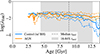 |
Fig. A.5. Eddington ratio AGN (orange) and non-AGN control (blue) samples as a function of the age of the Universe. The solid lines indicate the median evolution for the whole sample, while the dashed lines indicate the 16th and 84th percentiles. The vertical dashed line indicates the median black hole seeding time (AGN and non-AGN), and the shaded region encompasses the values between the 16th and 84th percentiles. The samples being compared here are 𝒮M* & M200cWBH and 𝒞M* & M200cWBH. |
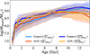 |
Fig. A.6. Comparison of neutral gas mass evolution between different AGN (shades of orange) and non-AGN control (shades of blue) samples. The horizontal axis shows the age of the Universe. The thick solid lines indicate the median evolution for the whole sample, while the shaded regions encompass the values between the 16th and 84th percentiles. |
Appendix B: Different AGN selection criteria
In this appendix, we explore how our main results, regarding the neutral gas component, are affected by changes in our AGN selection in the simulation. More specifically, changes involving the Eddington ratio.
As described in our Methods section, to select AGNs in TNG50-1, we used the Eddington ratio, more specifically, an average of this quantity over the last three snapshots in the simulation. However, we could also use the instantaneous value of the Eddington ratio to select the AGN. Thus, in Figure B.1 we show the histograms of the neutral gas mass for AGN-selected using instantaneous λEdd and its corresponding control sample of inactive dwarf galaxies (paired by stellar and halo mass). As it is clear from the figure, the AGNs still have lower masses than non-AGNs, regardless of the change in the selection method.
To test whether our main results on the neutral gas deficiency remain even if only the strongest AGNs are selected, similarly to Figure 7, we show in Figure B.1 the neutral gas masses of AGNs and non-AGNs. Additionally, in Figure B.2 we show the neutral-to-total gas mass fraction for dwarf galaxies in TNG50-1 with different values of λEdd. As it is clear from the figures, the general trend of our results remains the same if only dwarf AGNs with λEdd ≥ 0.05 are selected.
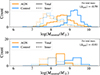 |
Fig. B.1. Histograms of neutral gas mass in the AGN and non-AGN control galaxies. Colors and line styles are as in the upper panel of Figure 7, but changing the selection criteria of AGN. The upper panel shows the mass distributions for AGN-selected using instantaneous λEdd, and the lower panel shows the mass distributions for AGN-selected using the λEdd, min = 0.05. The samples being compared here are 𝒮M* & M200cWBH and 𝒞M* & M200cWBH. |
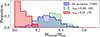 |
Fig. B.2. Histograms of neutral-to-total gas mass fraction for all central dwarf galaxies in TNG50-1 with stellar masses in the range 8 ≤ log(M*/M⊙)≤9.5. |
Appendix C: Other properties and environment measures
In this appendix, we present some extra physical quantities that were not presented in Section 3.2. The upper panel of Figure C.1 shows that all AGN samples are appropriately paired to their respective non-AGN control samples in stellar mass. Continuing from top to bottom in the panels of Figure C.1, we also show the stellar half-mass radius. This stellar radius is similar for AGN host and non-AGN galaxies once the halo mass is controlled. In the third panel from the top, we also present the neutral gas mass outside 2Re, *, which complements the results we found in Figure 6, with the neutral gas deficiency extending to the outskirts of active dwarf galaxies. In the last three lower panels of the figure, we show different distances to neighbors used to measure the environment. As it is clear from the information shown, no significant difference in environment is found once the halo mass is controlled.
 |
Fig. C.1. Same as Figure 4. From top to bottom the panels show box plots for: stellar mass, stellar half-mass radius, neutral gas mass outside 2Re, *, distance to the 10th nearest neighbor with M* ≥ 108 M⊙, distance to the 1st nearest neighbor with M* ≥ 1010 M⊙, distance to the 10th nearest neighbor with M* ≥ 1010 M⊙. |
Appendix D: Examples of AGN & non-AGN pairs
To illustrate the baryonic structures of the dwarf galaxies hosting AGNs and their matched control galaxies, we present a few maps of stellar and gas particles in Figure D.1. The few examples shown here reveal that the two-dimensional distribution of gas density and temperature can be very different between the AGN and non-AGN pairs of the simulations.
 |
Fig. D.1. Examples of three AGN-control pairs. Each row shows the different maps for a given galaxy in the face-on orientation, from left to right, the quantities are: stellar surface density (Σ*), gas surface density (Σgas), and gas temperature (T). Each two rows represent an AGN-control pair, with AGNs in the upper row and non-AGNs in the lower row for each pair. Stellar masses are indicated on the left of the maps. |
All Tables
All Figures
|
Fig. 1. Joint distribution of stellar (M*) and halo masses (M200c) for TNG50-1 central dwarf galaxies at z = 0. All 3297 dwarf galaxies are shown as blue squares, while the 789 dwarf galaxies hosting AGNs are shown as red diamonds. Density histograms represent the marginal distributions of samples in each axis. |
| In the text | |
|
Fig. 2. Scheme illustrating the samples referred to in this work. Numbers in parentheses indicate the number of galaxies. From the main sample of dwarf central galaxies in TNG50-1 (white ellipse), we created a sample of AGN hosts (red ellipse). We also created three parent samples of non-AGN galaxies (gray ellipses), one sample of galaxies with no restriction (NR) on their properties, another of galaxies with the restriction of having gas (WG), and another of galaxies with the restriction of having black holes (WBH). Specific non-AGN control samples (pink, green, and blue boxes) are thus drawn from these parent samples, while the corresponding AGN samples (orange boxes) are drawn from the sample of active dwarf galaxies (red ellipse). Dashed lines indicate the pairing of a specific non-AGN control sample and its respective AGN samples, following the method described in Section 2.5. The colors of the boxes of control samples indicate the variables used as control, and correspond to the same colors used in Figure 4. |
| In the text | |
|
Fig. 3. Fraction of central dwarf galaxies hosting AGNs according to different minimum thresholds for variables used in the sample selection. Top panel: AGN fraction as a function of the minimum threshold for λEdd. Bottom panel: AGN fraction as a function of the minimum threshold for stellar mass. In each panel, the solid lines show the fraction for different values of λEdd, min or M*,min, with the shaded regions representing the 95% confidence intervals. The red dashed lines indicate the overall fraction of dwarf AGN candidates from the DESI survey (Pucha et al. 2025), for the whole mass range of 8 ≲ log(M*/M⊙)≤9.5. This value (∼1.2%) is derived from the values presented in their figure 7 (right panel), and is the fraction of dwarf galaxies identified as AGN/Composite in the [N II]–BPT diagram, over the total number of dwarf galaxies (including dwarf galaxies without emission lines). |
| In the text | |
|
Fig. 4. Box plots of AGN (orange) and non-AGN control (pink, green, blue) sample properties. Each box extends from the first to the third quartile of the data, with a line at the median. The whiskers extend from the box edges to the farthest data point lying within 1.5 times the interquartile range from the box. Data past the end of the whiskers are shown as empty black circles. AGN samples are represented by orange boxes, control samples paired by M*, M* and SFR, or M* and M200c are represented by pink, green, and blue boxes, respectively. Different hatch patterns indicate the different parent samples of non-AGN central galaxies from which the control samples were constructed: no pattern, “x” pattern, and dot pattern refer to the “no restriction” (NR), “with gas” (WG), and “with BH”‘ (WBH) samples, respectively. The legend above the upper panel indicates the color and hatch pattern for each control sample shown in the figure. In each panel, above the boxes, we show the number of AGN hosts (NAGN), the difference between the median of the AGN and control (Δmed), and the p-value of an Anderson-Darling two-sample test performed with the control+AGN paired samples. In the cases where the difference was considered statistically significant (p-value < 0.05), the upper text is highlighted as bold and enclosed in a red box. From top to bottom, the panels show box plots for host halo mass, neutral-to-total gas ratio, and gas half-mass radius. |
| In the text | |
|
Fig. 5. Same as Figure 4, but (from top to bottom), the box plots show the specific star formation rate, stellar metallicity, median stellar formation time, and distance to the first-nearest neighbor (with M* ≥ 108 M⊙). |
| In the text | |
|
Fig. 6. Spherical gas profiles of AGN (orange) and non-AGN control (blue) samples. From top to bottom, we show the radial profiles of the volumetric gas density, the neutral-to-total gas mass ratio, and the gas temperature. In both panels, the thin semitransparent lines represent the profiles of individual galaxies, the thick solid lines represent the median profile of the whole sample, and the dashed lines indicate the 16th and 84th percentiles. The radial distance to the galaxy center (r) is rescaled by Re, *. The difference between median AGN and non-AGN profiles for a given quantity (Δ) is shown in black on the lower small sub-panels. The samples being compared here are 𝒮M* & M200cWG and 𝒞M* & M200cWG. |
| In the text | |
|
Fig. 7. Histograms of neutral, neutral atomic (H I), and molecular (H2) gas masses for the AGN (orange) and non-AGN control (blue) samples. The upper panel shows the bound neutral gas masses, with the solid line indicating the total amount and the dashed line indicating only the mass within 2Re, *. The middle and lower panels show the total bound gas masses in the form of H I and H2, taken from the TNG supplementary catalog (Diemer et al. 2019). Each line style of the histograms refers to a type of partition model considered by Diemer et al. (2019) in their post-processing: solid lines are from Gnedin & Draine (2014), dashed lines are from Gnedin & Draine (2014), dotted lines are from Krumholz (2013), and dotted-dashed lines are from Sternberg et al. (2014). Here, we show different models to illustrate variations in the values of MH I and MH2. In the upper right of each panel, we show the average pair-wise differences (Δpair) between the AGN and non-AGN logarithmic masses. The samples being compared here are 𝒮M* & M200cWG and 𝒞M* & M200cWG. |
| In the text | |
|
Fig. 8. Evolution of properties in AGN (orange) and non-AGN control (blue) samples. The time variable on the horizontal axis is the cosmic time minus the seeding time (tseed) of the AGN host. where the median tseed is 11 Gyr, and the 16th (84th) percentile is 7.3 Gyr (13 Gyr). From top to bottom and left to right, each panel represents the evolution of the neutral-to-total gas ratio, gas temperature, neutral gas mass, star formation rate, total gas mass, and host halo mass. All bound gas particles are considered. The solid lines indicate the median evolution of a given quantity for the whole sample, while the dashed lines indicate the 16th and 84th percentiles. Different from Figure 6, here we choose not to plot the data of each galaxy for better visualization. The samples being compared here are 𝒮M* & M200cWG and 𝒞M* & M200cWG. |
| In the text | |
|
Fig. 9. Examples of neutral-to-total gas profile evolution for a few AGNs selected at z = 0. In each panel, we show the profile of a specific galaxy at different times, before and after the black hole seeding. The two latest available profiles before tseed are shown as blue and gray solid lines, the earliest available profile after tseed is shown as a red solid line, and the present profile is shown as a black dotted line. The availability of the profiles depends on the type of simulation snapshot; see Section 2.3 for details. Each row is dedicated to a bin of black hole seeding times, in the top row tseed < 1 Gyr, and in the bottom row tseed > 3 Gyr. From left to right: Stellar mass of the example galaxies increasing in bins of roughly 0.25 dex. |
| In the text | |
|
Fig. 10. Top: histogram of AGN luminosities, bolometric (black), and total (0.5–10 keV) X-ray (green). Bottom: histogram of the ratio between AGN and X-ray binaries (XRB) luminosities. No extinction or obscuration is considered (see Section 2 for details on calculation). |
| In the text | |
|
Fig. 11. Median atomic-to-stellar mass ratio (MH I/M*) for AGNs (red stars) and non-AGNs (gray circles) in different stellar mass bins (upper panel) of TNG50-1. Error bars mark the 16th and 84th percentiles for each bin. The small lower panel indicates the difference between the medians of the AGN (λEdd ≥ 0.01) and non-AGN samples. The position of the markers on the x-axis corresponds to the median stellar mass of the galaxies in the bin. The number of objects in each mass bin is indicated by their corresponding colors. The samples of AGNs and non-AGNs are paired by stellar mass and contain only central galaxies. We also plot the MH I/M* values (red and gray solid lines) and uncertainties (shaded regions) reported on Ellison et al. (2019) (their Figure 8), which compares AGNs and non-AGNs in fixed stellar-mass bins. In the bottom panel, we show as a blue line the corresponding AGN-to-non-AGN difference from Ellison et al. (2019). |
| In the text | |
 |
Fig. A.1. Same as in Figure 7, but for the samples 𝒮M*WG and 𝒞M*WG. |
| In the text | |
 |
Fig. A.2. Same as in Figure 7, but for the samples 𝒮M* & M200cWBH and 𝒞M* & M200cWBH. |
| In the text | |
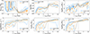 |
Fig. A.3. Same as in Figure 8, but for the samples 𝒮M* & M200cWBH and 𝒞M* & M200cWBH. |
| In the text | |
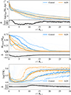 |
Fig. A.4. Same as in Figure 6, but for the samples 𝒮M* & M200cWBH and 𝒞M* & M200cWBH. |
| In the text | |
|
Fig. A.5. Eddington ratio AGN (orange) and non-AGN control (blue) samples as a function of the age of the Universe. The solid lines indicate the median evolution for the whole sample, while the dashed lines indicate the 16th and 84th percentiles. The vertical dashed line indicates the median black hole seeding time (AGN and non-AGN), and the shaded region encompasses the values between the 16th and 84th percentiles. The samples being compared here are 𝒮M* & M200cWBH and 𝒞M* & M200cWBH. |
| In the text | |
|
Fig. A.6. Comparison of neutral gas mass evolution between different AGN (shades of orange) and non-AGN control (shades of blue) samples. The horizontal axis shows the age of the Universe. The thick solid lines indicate the median evolution for the whole sample, while the shaded regions encompass the values between the 16th and 84th percentiles. |
| In the text | |
|
Fig. B.1. Histograms of neutral gas mass in the AGN and non-AGN control galaxies. Colors and line styles are as in the upper panel of Figure 7, but changing the selection criteria of AGN. The upper panel shows the mass distributions for AGN-selected using instantaneous λEdd, and the lower panel shows the mass distributions for AGN-selected using the λEdd, min = 0.05. The samples being compared here are 𝒮M* & M200cWBH and 𝒞M* & M200cWBH. |
| In the text | |
|
Fig. B.2. Histograms of neutral-to-total gas mass fraction for all central dwarf galaxies in TNG50-1 with stellar masses in the range 8 ≤ log(M*/M⊙)≤9.5. |
| In the text | |
|
Fig. C.1. Same as Figure 4. From top to bottom the panels show box plots for: stellar mass, stellar half-mass radius, neutral gas mass outside 2Re, *, distance to the 10th nearest neighbor with M* ≥ 108 M⊙, distance to the 1st nearest neighbor with M* ≥ 1010 M⊙, distance to the 10th nearest neighbor with M* ≥ 1010 M⊙. |
| In the text | |
|
Fig. D.1. Examples of three AGN-control pairs. Each row shows the different maps for a given galaxy in the face-on orientation, from left to right, the quantities are: stellar surface density (Σ*), gas surface density (Σgas), and gas temperature (T). Each two rows represent an AGN-control pair, with AGNs in the upper row and non-AGNs in the lower row for each pair. Stellar masses are indicated on the left of the maps. |
| In the text | |
Current usage metrics show cumulative count of Article Views (full-text article views including HTML views, PDF and ePub downloads, according to the available data) and Abstracts Views on Vision4Press platform.
Data correspond to usage on the plateform after 2015. The current usage metrics is available 48-96 hours after online publication and is updated daily on week days.
Initial download of the metrics may take a while.