| Issue |
A&A
Volume 705, January 2026
|
|
|---|---|---|
| Article Number | A193 | |
| Number of page(s) | 18 | |
| Section | Interstellar and circumstellar matter | |
| DOI | https://doi.org/10.1051/0004-6361/202557609 | |
| Published online | 23 January 2026 | |
Zooming into the water snow line: High-resolution water observations of the HL Tau disk
1
Dipartimento di Fisica, Università degli Studi di Milano,
Via Celoria 16,
20133
Milano,
Italy
2
Departamento de Astronomía, Universidad de Chile,
Camino El Observatorio
1515,
Las Condes, Santiago,
Chile
3
Max-Planck-Institut für Astronomie,
Königstuhl 17,
67117
Heidelberg,
Germany
4
INAF – Istituto di Radioastronomia,
Via Gobetti 101,
40129
Bologna,
Italy
5
European Southern Observatory (ESO),
Karl-Schwarzschild-Straße 2,
85748
Garching bei München,
Germany
★ Corresponding author: This email address is being protected from spambots. You need JavaScript enabled to view it.
Received:
8
October
2025
Accepted:
19
November
2025
Abstract
Context. Water is one of the central molecules for the formation and habitability of planets. In particular, the region where water freezes out, the water snow line, could be a favorable location for planets to form in protoplanetary disks.
Aims. We aimed to spatially resolve the water emission in the HL Tau disk using high-resolution ALMA observations of the H2O 183 GHz line (Eu = 205 K). We compared the spatially resolved H2O emission with that of H13CO+, a chemical tracer of the water snow line, to observationally test their anticorrelation. In addition, we aimed to quantify the fraction of the water reservoir hidden by optically thick dust at ALMA wavelengths versus far- and mid-IR wavelengths.
Methods. We used high-resolution ALMA observations to spatially resolve the H2O 31,3–22,0 line at 183 GHz, H13CO+ J = 2–1, and the SO 44–33 transition in the HL Tau disk. A rotational diagram analysis was used to characterize the water reservoir seen with ALMA and compare it to the reservoir visible at mid- and far-IR wavelengths.
Results. We find that the H2O 183 GHz line has a compact central component and a diffuse component that is seen out to ∼75 au. A radially resolved rotational diagram shows that the excitation temperature of the water is ∼350 K, independent of radius. The steep drop in the water brightness temperature outside the central beam of the observations where the emission is optically thick is consistent with the water snow line being located inside the central beam (≲6 au) at the height probed by the observations. Comparing the ALMA lines to those seen at shorter wavelengths shows that only 0.02–2% of the water reservoir is visible at mid- and far-IR wavelengths due to optically thick dust hiding the emission, whereas 35–70% is visible with ALMA. An anticorrelation between the H2O and H13 CO+ emission is found, but it is likely caused by optically thick dust hiding the H13CO+ emission in the disk center. Finally, we see SO emission tracing the disk and, for the first time in SO, a molecular outflow and the infalling streamer out to ∼2′′. The velocity structure hints at a possible connection between the SO and the H2O emission.
Conclusions. Spatially resolved observations of H2O lines at (sub)millimeter wavelengths provide valuable constraints on the location of the water snow line while probing the bulk of the gas-phase reservoirs.
Key words: astrochemistry / protoplanetary disks / stars: individual: HL Tau / submillimeter: planetary systems
© The Authors 2026
 Open Access article, published by EDP Sciences, under the terms of the Creative Commons Attribution License (https://creativecommons.org/licenses/by/4.0), which permits unrestricted use, distribution, and reproduction in any medium, provided the original work is properly cited.
This article is published in open access under the Subscribe to Open model. This email address is being protected from spambots. You need JavaScript enabled to view it. to support open access publication.
1 Introduction
Water has been a key molecule in the shaping of our Solar System. On a very local scale, water is essential for the life on Earth we know today. On the scale of (our) planetary system, the water snow line, where water freezes out in the protoplanetary disk, could have been a favorable location for planets to start forming (Drążkowska & Alibert 2017; Schoonenberg & Ormel 2017). In addition, water is one of the main carriers of oxygen. Therefore, there is a major shift in the oxygen reservoir from gas to ice across the water snow line, which changes the chemical composition of the planet-forming material (Öberg et al. 2011; Öberg & Bergin 2021).
Locating the water snow line in a protoplanetary disk is difficult. In a typical disk around a T Tauri or Herbig star, the snow line is located at a radius of a few up to ∼10 au from the central star (Harsono et al. 2015). Thus, ground-based observatories, such as the Atacama Large Millimeter/submillimeter Array (ALMA), that can reach the required angular resolution have to look through the Earth’s atmosphere, where gas-phase water can absorb the water emission from a protoplanetary disk or other astronomical objects.
Space based-observatories such as Spitzer, Herschel, and JWST are not limited by the water in the Earth’s atmosphere but lack the spatial resolution to resolve the water snow line. Still, some constraints on the water snow line location have been obtained by analyzing spectrally resolved line profiles (e.g., Pontoppidan et al. 2010; van Dishoeck et al. 2021; Pirovano et al. 2022; Banzatti et al. 2025). In addition, the water emission can be characterized through a rotational diagram analysis or with thermochemical models (e.g., Pirovano et al. 2022; Pontoppidan et al. 2024; Banzatti et al. 2023; Gasman et al. 2023; Temmink et al. 2024; Kaeufer et al. 2024; Vlasblom et al. 2025). These methods can be used to distinguish the three water reservoirs in disks: (1) the thermally desorbed water reservoir at a temperature of 150 K inside the water snow line, (2) the cold photo-desorbed reservoir in the outer disk below the sublimation temperature of water, and (3) the reformed water in the disk surface layers where the gas temperature exceeds 300 K such that OH can react with H2 to form H2O.
To circumvent the Earth’s atmosphere and probe closer to the disk midplane, chemical tracers of the water snow line have been observed with, for example, ALMA. From a chemical point of view, HCO+, or the more optically thin H13CO+ isotopologue, is one of the best tracers of the water snow line since it is very effi-ciently destroyed by gas-phase H2O (Phillips et al. 1992; Bergin et al. 1998). Therefore, no HCO+ emission is expected in the disk center, and a ring of emission is seen outside the water snow line where HCO+ can survive (Leemker et al. 2021). Still, optically thick dust complicates the analysis of HCO+ observations as it can also cause a central hole in the molecular line emission (Isella et al. 2016; Weaver et al. 2018). Therefore, HCO+ isotopo-logues are best used in disks with optically thin dust around the water snow line (Leemker et al. 2021).
Recently, the water snow line has been located directly through emission of H2O or its isotopologues in three bright disks. Spatially resolved emission of HDO and  in the disk around the young, outbursting V883 Ori star drops off at 80 au, confirming the results from other chemical tracers and detailed modeling (van ’t Hoff et al. 2018; Leemker et al. 2021; Tobin et al. 2023; Wang et al. 2025). The main water isotopologue has been used in the disk around the highly accreting AS 205 star, where the water snow line was found to be vertical at a radial distance of 2 au via modeling of the line profile of a high excitation line (1861.3 K upper energy level; Carr et al. 2018; Bosman & Bergin 2021). In the HD 100546 disk, the snow line was found to be at the dust cavity wall (Rampinelli et al. 2026).
ALMA has the potential to resolve the water snow line in quiescent disks without a central cavity via the H2O 183 GHz line. This line has an upper energy level comparable to the sublimation temperature of water (Eu = 205 K) and thus probes the thermally desorbed water reservoir. Facchini et al. (2024) published the first, and to date only, detection of this line in a full and quiescent disk: HL Tau. In this work, we combined these data with new high-resolution observations of this line. HL Tau is a massive Class I/II protoplanetary disk of 0.2 M⊙ surrounded by a protostellar envelope at a distance of 140 pc (Rebull et al. 2004; Robitaille et al. 2007; Furlan et al. 2008; Galli et al. 2018; Booth & Ilee 2020). In addition, a streamer is seen in HCO+ that impacts the disk, liberating SO and SO2 (Yen et al. 2019; Garufi et al. 2022), although no CH3OH is detected (Soave in prep.). In the mid- and far-IR, hot gas-phase water is detected (Riviere-Marichalar et al. 2012; Alonso-Martínez et al. 2017; Salyk et al. 2019) that likely originates from the inner regions of the highly structured dust disk (ALMA Partnership 2015; Carrasco-González et al. 2019; Guerra-Alvarado et al. 2024).
In Sect. 2, the self-calibration of these data is described together with the H13CO+ and SO lines that are detected in the same dataset. Our results are presented in Sect. 4, where we observationally test the H2O–HCO+ anticorrelation due to the water snow line. In addition, we compare the water reservoir visible with ALMA at (sub)millimeter wavelengths to that in the mid- and far-IR. In Sect. 5 the implications for the water snow line location are discussed, and the morphologies of the H2O and SO emission are compared. Our conclusions are summarized in Sect. 6.
2 Observations
The main water isotopologue in the HL Tau disk has been targeted by two separate ALMA projects. In this work we present new, high-spatial-resolution data of the H2O line at 183 GHz in ALMA Band 5 that was observed as part of ALMA project 2022.1.00905.S (PI: S. Facchini, Facchini et al. 2024). These data were combined with ALMA program 2017.1.01178.S data (PI: E. Humphreys, Facchini et al. 2024), which there taken in a more compact configuration to increase the maximum recoverable scale of the combined dataset. In addition, we reimaged the self-calibrated H2O 321 GHz line in ALMA Band 7 observed by the latter program to allow for a uniform analysis with the 183 GHz line. The calibration of these data is presented in Facchini et al. (2024).
HL Tau was observed in the compact configuration for 1.6 hours, corresponding to a single execution block (EB). The spectral setup included a spectral window (spw) centered at the p-H2O 313–220 transition at 183.310 GHz with a spectral resolution of 122 kHz (0.2 km s−1). In addition, a continuum spw centered at 170.004 GHz with a spectral resolution of 977 kHz (1.7 km s−1) and four spws centered at 172.117 GHz, 172.709 GHz, 181.334 GHz, and 182.445 GHz with a spectral resolution of 122 kHz (0.2 km s−1) were included.
The long-baseline data (2022.1.00905.S) consist of seven EBs of 1.7 hours each including calibration. These data cover the same H2O 183 GHz line at the same spectral resolution but also included a spw with a resolution of 122 kHz (0.2 km s−1) centered at the H13CO+ J = 2–1 transition at 173.507 GHz (Eu = 12.5 K). In addition, the SO 44–33 transition at 172.181 GHz (Eu = 33.7 K) is covered in the continuum spw centered at 171.525 GHz (977 kHz or 1.7 km s−1 spectral resolution). A second continuum spw was centered at 185.525 GHz. An overview of both programs is presented in Table 1.
We redid the self-calibration of the data, covering the H2O 183 GHz in the compact configuration (2017.1.01178.S), and we jointly self-calibrated them with the data taken in the extended configuration (2022.1.00905.S) following the methods of the exoALMA large program (Loomis et al. 2025) using modules by Andrews et al. (2018); Czekala et al. (2021). We used CASA version 6.5.4 (McMullin et al. 2007; CASA Team 2022). Before starting the self-calibration, the data within 15 km s−1 of the H2O 183 GHz line and other bright lines were flagged after visual inspection of the data. This resulted in a total continuum bandwidth of 2.4 GHz for the short-baseline (SB) and 4.2 GHz for the long-baseline (LB) data. In addition, a phase-shift was applied to the high-resolution data to align it with the low-resolution data using the phaseshift task in CASA. The coordinate system was fixed to the new phase center using the task fixplanets.
A single round of phase-only self-calibration was applied to each EB of the short- and long-baseline data separately. A model was created by cleaning the emission in each EB down to a 6σ threshold using the task tclean. The phase-only gain solutions were found using the gaincal task where spws, scans, and polarizations were combined to a solution interval with the length of a single EB. In addition, only the antennas with at least three baselines and gain solutions with a signal-to-noise ratio of at least four were included. These solutions were applied to the data with applycal in the “calonly” mode. All long-baseline EBs were then aligned with respect to the EB that was observed with the highest signal-to-noise ratio using the exoALMA alignment procedure (Loomis et al. 2025). The short-baseline data were aligned with the seven concatenated long-baseline EBs.
Before combining the short and long-baseline data, the phases of the short-baseline data were self-calibrated in five subsequent rounds with decreasing solution intervals with the length of a single EB, 360, 120, 60, and 20 seconds. During the first round separate solutions were found for both polarizations whereas in the subsequent rounds the polarizations were combined to improve the signal-to-noise ratio on the solutions. This improved the peak signal-to-noise ratio on the continuum from 955 to 2682.
The resulting self-calibrated short-baseline data were combined with the long-baseline data for a single round of phase-only joint self-calibration. The solution interval for this round was set to the length of a single EB when combining spws and scans, and separate solutions were found for the two polarizations. Additional rounds of self-calibration did not lead to an improvement in the signal-to-noise ratio of the resulting continuum image. Comparing the total flux revealed that the flux measured in all EBs are within 4% of that in LB EB3 except for LB EB 2. Following Loomis et al. (2025), we rescaled the flux in this EB and repeated the joint short- and long-baseline self-calibration.
Finally, we performed two rounds of amplitude and phase-self-calibration on the data. The models for these rounds of self-calibration were obtained by cleaning the image down to a 1σ threshold to include as much flux as possible in the model. Then solutions were found for EB- and scan-long intervals by combining spws, scans, and polarizations and by combining solely spws and polarizations, respectively. This increased the peak signal-to-noise ratio on the continuum from 1102 after the SB self-calibration but before the joint self-calibration to 1365 after the joint self-calibration.
The gain solutions of the self-calibration were applied to the data containing the lines following the same order of the procedures as during the self-calibration. The data were continuum-subtracted using the CASA task uvcontsub_old by fitting a first-order polynomial to the line free channels.
ALMA observations covering the H2O line at 183 GHz.
2.1 Imaging
The data were imaged with the CASA task tclean using Briggs weighting. As the continuum is seen at a very high peak signal-to-noise ratio of 1365 when imaged with a robust parameter of 0.5 used for the self-calibration, the final continuum image is made with a robust parameter of −0.5, providing a high spatial resolution of 0′′.056 × 0′′.035 (−38.7°) without losing too much in the signal-to-noise ratio. The continuum flux density within a 1′′.0 radius circular region centered on the continuum peak is 335±34 mJy, where the uncertainty is dominated by the absolute flux calibration uncertainty of ALMA.
The water line is weaker and therefore imaged with a robust parameter of 0.0 and 2.0 and a channel width of 1 km s−1. The small robust parameter of 0.0 provides a very good spatial resolution of 0′′.083 × 0′′.066 (−21.0°) at the cost of a larger channel rms noise. The weighting scheme with a robust parameter of 2.0 provides a much larger beam of 0′′.35 × 0′′.30 (−8.5°), increasing the sensitivity to the diffuse H2O emission at larger spatial scales (see the top-right and bottom-right panel in Fig. 1). The channel rms of these cubes is frequency-dependent due to telluric around the targeted H2O line. Therefore, the noise in each channel depends on the position of that channel with respect to the telluric at the time of the observations. We refer the reader to Appendix A.1 and Rampinelli et al. (2026) for a detailed discussion. The H2O channel maps are presented in Figs. A.2 and A.3; those in the former are imaged at a spectral resolution of 5 km s−1 to increase the signal-to-noise ratio in the channel maps.
The H13CO+ was only covered by the long-baseline data. The H13CO+ J = 2–1 line (Eu = 12.5 K) was imaged in 1 km s−1 wide channels with a robust parameter of 2.0 and a 0′′.2 uv-taper to increase the sensitivity to extended emission. This resulted in a cube with a channel rms of 0.7 mJy beam−1.
The SO 44 − 33 line (Eu = 33.7 K) was covered by the continuum spw in the long-baseline data only, and was imaged with a robust parameter of 0.5 and a channel width of 2 km s−1. As this line is far from the center of the telluric, the resulting channel rms of the SO cube is only 0.3 mJy beam−1.
Finally, we reimaged the H2O line at 321 GHz using the self-calibrated ms tables of Facchini et al. (2024) to allow for a uniform analysis of the data. The continuum-subtracted image was recreated following Facchini et al. (2024) but with a 1 km s−1 channel width, resulting in a channel rms of 2 mJy beam−1. Non-continuum-subtracted images to measure the brightness temperature of the H2O 183 GHz and 321 GHz lines were made following the same procedure that was used for the continuum-subtracted images.
2.2 JvM-correction
In order to accurately retrieve line fluxes and channel map intensities, we applied the so-called Jorsater–van Moorsel (JvM) correction to the line cubes (Jorsater & van Moorsel 1995). As detailed in Czekala et al. (2021), this is needed in order not to overestimate line fluxes for extended and low signal-to-noise ratio emission morphologies, where a large fraction of the emission is not included in the clean model. In our paper, this is particularly important for the water line flux measurements. We verified that this correction is needed to maintain the uniform line fluxes across a wide range of robust parameters used in tclean. We note that Facchini et al. (2024) did not apply the JvM correction and thus overestimated the 321 GHz water line flux. The 183 GHz water line in Facchini et al. (2024) is significantly less affected due to the higher signal-to-noise ratio in the SB data. Since the JvM correction is known to underestimate the point source rms (Casassus & Cárcamo 2022), uncertainties on flux measurements are estimated on the non-JvM-corrected images (Sect. 3.2). The so-called ϵ factors (used to rescale the residuals in the clean image restoration) are reported in Table 2.
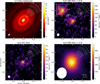 |
Fig. 1 ALMA Band 5 images of the HL Tau disk and the 321 GHz H2O line. Top left: continuum. Right panels: JvM-corrected integrated intensity maps of the H2O line at 183 GHz imaged with r = 0.0 (top) and r = 2.0 (bottom). These maps provide high and moderate spatial resolution. Top-right inset: zoomed-in view of the inner 0′′.2. This highlights the approximate water snow line location derived by Guerra-Alvarado et al. (2024) Bottom left: reimaged H2O 321 GHz line originally presented in Facchini et al. (2024). The beams are indicated in the bottom-left corners of the respective panels. The dust rings and gaps derived from high-resolution ALMA observations are indicated with solid and dashed arcs in each panel (ALMA Partnership 2015; Carrasco-González et al. 2019; Guerra-Alvarado et al. 2024), and a 20 au scale bar is shown in the bottom-right corner of the bottom-right panel. |
3 Methods
To further analyze the data, the image cubes were collapsed to moment maps and spectra, as described below. In addition, the rotational diagram analysis to derive column densities is briefly reiterated.
3.1 Moment maps and integrated fluxes
The moment 0, 1, and 8 maps are computed using the Better Moments package (Teague 2019). No clip was applied to the integrated and peak intensity maps (moment 0 and 8) and a 4σ clip was applied to the cubes before obtaining the moment 1 maps. In addition, a Keplerian mask was applied to the H13CO+ cube before making the integrated intensity map as this line was found to generally follow a Keplerian pattern (see Fig. A.7). This mask predicts where the H13CO+ emission emits in the channel maps based on the disk inclination of 46.7°, the position angle of 138°, a distance of 140 pc, a stellar mass of 2.1 M⊙, and the source velocity of 7.1 km s−1 (Rebull et al. 2004; ALMA Partnership 2015; Galli et al. 2018; Yen et al. 2019; Garufi et al. 2021, 2022). The outer radius of the mask is set to a large radius of 20′′ to include all flux. Finally, the mask is convolved with a Gaussian 1.5 times larger than the beam.
The maps of the H2O lines were created by integrating the cubes from –8.5 to 22.5 km s−1 for the 183 GHz line and from –10.4 to 24.6 km s−1 for the 321 GHz line. The latter velocity range is identical to that in Facchini et al. (2024), but the former is larger as the 183 GHz line is detected out to higher velocity offsets from the systemic velocity of 7.1 km s−1 with the addition of the long-baseline data. The H13CO+ and SO emission are integrated over a range from –8.5 to 22.5 km s−1 and from –5 to 19 km s−1, respectively.
The disk-integrated fluxes were computed using the same velocity limits as were used for the moment maps. We note that the H13CO+ and the SO emission in the channel maps extend to scales up to or beyond the maximum recoverable scale of 1′′.7 of the long-baseline data (see Figs. A.6 and A.9). Therefore, some flux might be resolved out. An overview of the detected lines is presented in Table 2.
Observed molecular lines with ALMA in the HL Tau disk.
3.2 Uncertainties on the disk-integrated flux and azimuthally averaged radial profiles
The uncertainty on the disk-integrated flux was estimated by propagating the channel rms from the non-JvM-corrected cube:
 (1)
(1)
with σchan the rms in the channels, ∆Vchan the channel width, Npix mask the total number of pixels in space and velocity used to calculate the integrated flux (Fν∆V), and Npix beam the number of pixels per beam. The 10% absolute flux calibration uncertainty of ALMA is added in quadrature.
Similarly, the uncertainty on the azimuthally averaged radial profiles obtained using the gofish package (Teague 2019) were estimated from the channel rms. First, the uncertainty map of the integrated intensity was estimated following, for example, Leemker et al. (2023):
 (2)
(2)
with Nchan the number of channels the integrated intensity map is computed over. If a Keplerian mask is used, Nchan depends on the location in the map, with positions close to the star generally having more channels than those farther away. The uncertainty in each bin of the azimuthally averaged radial profile then follows
 (3)
(3)
with Nbeams per bin the number of beams per bin and Npix per bin the number of pixels in each radial bin. As the bins have a width of a quarter of the beam major axis, the number of beams per bin is calculated as the ratio of the circumference of the ellipse that defines the radial bin and the average of the beam major and minor axes.
3.3 Rotational diagram
The resulting H2O 183 GHz line is imaged at a similar spatial scale to the 321 GHz line originally presented in Facchini et al. (2024). As these lines have different upper energy levels, the ratio of their observed flux is a probe of their excitation temperature when convolved to the same beam size. As the 321 GHz line is observed at a slightly higher spatial resolution, this cube is convolved to match the beam size of the 183 GHz line.
The formalism by Goldsmith & Langer (1999) and Loomis et al. (2018) is briefly summarized below. If the emission is optically thin, the integrated flux is directly related to the column density of the upper level (u) as
 (4)
(4)
with Aul the Einstein-A coefficient for spontaneous emission, Ω the assumed emitting region, h the Planck constant, and c the speed of light. For the radially resolved rotational diagram, the emitting area is assumed to be the beam size.
For (marginally) optically thick lines, the assumption of optically thin emission leads to an underestimation of the column density of level u by a factor of C(τν):
 (5)
(5)
 (6)
(6)
with τν the optical depth of the line. This can be approximated as
 (7)
(7)
with ν the frequency of the line, kB the Boltzmann constant, T the excitation temperature, and  the thermal line width for a molecule of mass m.
Under the assumption of local thermodynamical equilibrium (LTE), the level populations follow a Boltzmann distribution:
 (8)
(8)
with gu and Eu the degeneracy and energy of level u, respectively, Ntot the total water column density, and Q(T) the partition function. An overview of the disk-integrated line fluxes is presented in Table 2 for the lines observed with ALMA and in Table 3 for all H2O lines seen in the HL Tau disk with ALMA, Herschel, and Gemini North. In addition, Table 3 includes the line constants for the H2O transitions analyzed in this work. The constants for the lines observed with ALMA and Herschel were taken from the JPL database (Pickett et al. 1998; Yu et al. 2012). However, constants for the high excitation lines seen with Gemini North are not included in the JPL database; they were therefore taken from the LAMDA database (Tennyson et al. 2001; Schöier et al. 2005; Barber et al. 2006; Faure & Josselin 2008) where gu is corrected for the assumed ortho-to-para ratio of 3 used by the partition function in the JPL database and appropriate for H2O that formed in the gas-phase or was thermally desorbed (Cheng et al. 2022).
The uncertainty on the temperature, column density, and optical depth is estimated from the uncertainty on the integrated flux including the 10% absolute flux calibration uncertainty of ALMA as the H2O lines are part of different ALMA projects and compared to lines seen with Herschel and Gemini North. First, the uncertainty on the temperature is estimated. As the temperature cannot be isolated in Eq. (8) due to the dependence in Nu, Q(T), and  , the equation is linearized through a first-order Taylor polynomial around
  :
:
 (9)
(9)
where f is defined as
 (10)
(10)
with subscripts 1 and 2 referring to the two lines used for the rotational diagram analysis. The uncertainty on T is then estimated using the standard propagation of uncertainty on Eq. (9) where the derivatives are calculated numerically over a 5% step size in each parameter. The uncertainty on Ntot and τν are estimated using the standard propagation of uncertainty on Eqs. (7) and (8) taking the error on the temperature and integrated flux into account.
Disk-integrated H2O line fluxes in the HL Tau disk.
4 Results
4.1 H2O morphology
The self-calibrated continuum image and the integrated intensity maps of the H2O 183 GHz and 321 GHz lines are presented in Fig. 1. The H2O emission imaged with a small robust parameter of 0.0 providing high angular resolution and good sensitivity to point sources is presented in the middle panel. The emission is compact and peaks at a projected distance of 5 au in the southwest, consistent with the center of the disk within the size of the beam of 0′′.083 × 0′′.066 (12 × 9 au). Following Fasano et al. (2025), the significance of this offset can be estimated using the uncertainty on the astrometric accuracy: θFWHM/(0.9×S/N), with θFWHM the size of the beam and S/N the signal-to-noise ratio of the peak that we conservatively measured using the peak integrated intensity in the JvM-corrected moment 0 map and the noise in the non-JvM-corrected map. As the astrometric uncertainty of 0′′.03 is comparable to 5 au projected distance, the offset is not significant at the signal-to-noise ratio of the data.
The H2O 183 GHz integrated intensity map imaged at a higher robust parameter of 2.0 is presented in the right hand panel. The water emission in this panel is seen out to much larger radii due to the better sensitivity to diffuse and extended emission. Still, the H2O emission is more compact than the continuum disk. A slight asymmetry is seen in the H2O emission when imaged at moderate angular resolution where the diffuse water emission extends somewhat toward the north or northeast side of the disk.
The azimuthally averaged radial profiles of the high-resolution H2O 183 GHz and 321 GHz lines together with that of the continuum emission are presented in the left panel of Fig. 2. The H2O 183 GHz line is centrally peaked with a steep drop off outward. Imaging the H2O 183 GHz line with higher robust parameters and thus larger beam sizes that are more sensitive to diffuse emission, reveals that the water emission extends out to ∼75 au (see Fig. A.5). Similarly, the hot 321 GHz line shows a bright central component and an extended shoulder of emission between ∼10 and 40 au. This suggests that the central component of the H2O 183 and 321 GHz lines probes a large column of gas-phase H2O inside the water snow line.
This is further supported by the brightness temperature profiles of the lines that are presented in the right panel of Fig. 2 derived using the Rayleigh-Jeans approximation and the peak intensity map extracted from the image cube between −8.5 km s−1 and 22.5 km s−1 without continuum subtraction and without shifting each pixel by the project Keplerian velocity at that location. Similar to the integrated intensity profiles, the shifting and stacking was not applied as this can underestimate the intensity in the inner disk regions where the water snow line is expected to be located. The brightness temperature profiles are only shown in the inner 50 au because the peak intensity in the outer disk regions is dominated by the noise in the data cubes as the peak flux is measured over a large velocity range. The H2O 183 GHz and 321 GHz lines reach a high brightness temperature of 220 K and 160 K in the inner beam, respectively. These temperatures are a lower limit to the kinetic temperature of the gas due to the finite line optical depth, spatial, and spectral resolution of the data (Leemker et al. 2022) and assume LTE emission. Therefore, the gas probed by the central beam of the observations is sufficiently warm for thermal sublimation of water inside the water snow line at T ∼ 150 K. Outside the central beam, the brightness temperature steeply drops, suggesting that the water becomes less optically thick.
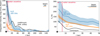 |
Fig. 2 Azimuthally averaged radial profiles of the integrated intensity (left) and brightness temperature (right). The H2O line at 183 GHz imaged with a robust parameter of 0.0 is indicated in blue, the H2O line at 321 GHz in orange, and the continuum emission in black. In the left panel the continuum emission is presented in arbitrary units, and the upper limit on the water snow line location is indicated with the vertical red line. Note the difference in the radial axes. The beams are indicated with the horizontal bars in the top-right corner. |
4.2 Excitation of H2O at submillimeter wavelengths
To analyze the origin of the water in the HL Tau disk, we performed a rotational diagram analysis using the warm 183 GHz and the hot 321 GHz line with upper energy levels of 205 K and 1861 K, respectively. The integrated intensity map of the 321 GHz line was convolved to the beam size of the 183 GHz line to compare the lines on the same spatial scale. The results assuming LTE are presented in Fig. 3. The column density derived from the 183 and 321 GHz lines are identical by construction though their uncertainties are not due to the dependence on the uncertainty on the excitation temperature and the line flux itself. The assumption of LTE is further discussed in Sect. 4.3.
The excitation temperature of the H2O line is ∼350 K and independent of radius within the uncertainty of the data. Following the results from the radial profiles, the rotational diagram can be divided into two regions: the inner beam where the 183 GHz line is optically thick and remaining disk regions. In the inner regions, the optical depth of the 183 GHz line is an order of magnitude higher than that of the 321 GHz line though the precise value is uncertain; see the right panel Fig. 3. As the warm 183 GHz line is more optically thick than the hot 321 GHz line, the rotational temperature in the inner beam overestimates the kinetic temperature of the H2O gas. Therefore, the inner beam likely probes a large column of gas-phase H2O at a temperature of at most 350 K, consistent with the thermally desorbed water reservoir. As the lines are (marginally) optically thick in this region, the observations likely do not probe the disk mid-plane. Thus, the water snow line is likely located inside the inner beam (≲6 au) at the height in the disk probed by the observations.
Outside the central beam, the emission is less optically thick as the brightness temperature drops well below the excitation temperature. The excitation temperature of 350 K is consistent with the expected temperature of 300 K above which water can reform from OH. Therefore, the emission is likely tracing the radially extended warm water reservoir in the disk surface.
The column density and excitation temperature derived from the high-resolution 183 and 321 GHz data presented in this work are roughly consistent with those derived from these lines and the 325 GHz line at lower spatial resolution in Facchini et al. (2024). Their H2O column density assuming that all emission originates from within 17 au is consistent with that in the inner beam within a factor of 2. The excitation temperatures are somewhat different due to the overestimation of the flux of the hot 321 GHz line (see Sect. 2.2) and the addition of the 325 GHz line (Eu = 470 K) in Facchini et al. (2024) that is only available at low spatial resolution and thus not included in the analysis presented in this work.
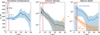 |
Fig. 3 Radially resolved rotational diagram analysis of the H2O emission in the HL Tau disk. The excitation temperature (left), column density (middle), and optical depth (right) of the H2O 183 GHz (blue) and 321 GHz (orange) lines are obtained after convolving the two lines to the same beam size. The dashed lines are derived under the assumption of fully optically thin emission, whereas the solid lines include the correction for the optical depth of the lines. The black scatter points indicate the disk-averaged results from Facchini et al. (2024) assuming an emitting region of 17 au; the upper limit on the water snow line location is indicated with the vertical red line. |
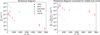 |
Fig. 4 Rotational diagram summarizing the disk-integrated H2O line detections in the HL Tau disk with ALMA in the (sub)millimeter (cyan), Herschel PACS in the far-IR (pink), and Gemini North in the mid-IR (orange). Left: rotational diagram without a correction for the difference in the continuum optical depth for the various lines. Right: rotational diagram with a correction factor derived from a thermochemical model. The shaded points in the right panel are identical to the non-shaded points in the left panel. |
4.3 H2O hidden by optically thick dust
The H2O 183, 321, and 325 GHz lines are the only two spatially resolved water lines detected in the HL Tau disk to date. However, water has been detected in this disk before at a lower angular resolution with other observatories such as Herschel, Gemini North, the Submillimeter Array (SMA), and ALMA (Riviere-Marichalar et al. 2012; Kristensen et al. 2016; Alonso-Martínez et al. 2017; Salyk et al. 2019; Facchini et al. 2024). A rotational diagram of these lines assuming an ortho-to-para ratio of 3 is presented in the left panel of Fig. 4. The H2O line detected with the SMA is not included in this diagram as it is shifted by –20 km s−1 with respect to the source velocity of HL Tau, whereas this line observed with ALMA is centered around the systemic velocity, suggesting that the H2O line observed with the SMA does not trace the same emission as the other water lines (Kristensen et al. 2016; Facchini et al. 2024). The column densities of the upper level are derived by assuming a 17 au emitting region in the disk frame, following the upper limit on the snow line location (Facchini et al. 2024). A different emitting region will shift all data points by a constant factor that is the ratio of the emitting regions but it does not change the relative differences between the data points. An overview of all the lines and the line parameters used is presented in Table 3.
The rotational diagram shows a 2–3 order of magnitude difference between the column density of the H2O lines observed with ALMA and those observed with Herschel despite the upper energy levels being similar (Fig. 4, left). Two possible causes for this difference include masing of the 183, 321, and 325 GHz lines seen with ALMA and water emission being hidden by optically thick dust. These ALMA lines are known to be potential masers if the gas density is lower than ∼1010 cm−3 and, in the case of the 321 GHz line, a temperature exceeding ∼500 K (Gray et al. 2016). In this case, the assumption of LTE to convert the line flux to a column density is no longer valid and the derived column density overestimates the true column density due to the population inversion.
To investigate the second option, we made a simple thermochemical DALI model of a full disk that reproduces the continuum and CO isotopologue flux seen in the HL Tau disk with ALMA within a factor of 2 for most disk regions (see Appendix B for details). We note that the first dust gap in the HL Tau disk lies at 13 au, which is outside the predicted water snow line location (2 au) for this model (black contour in Fig. 5). For each of the lines in Fig. 4, the position in radius r and height z of the τdust = 1 surface is computed. As the continuum optical depth decreases with increasing wavelength, this surface shifts to layers deeper in the disk, revealing more of the water reservoir at longer wavelengths; see Fig. 5. The fraction of the gas-phase H2O molecules above that surface  compared to the total number of gas-phase H2O molecules in the disk (𝒩tot in disk) is a measure for the amount of water hidden below the optically thick dust (see Table 3). The H2O line fluxes themselves are not compared as a number of lines are predicted to be masing in some regions of the disk, which is artificially quenched in DALI by limiting their optical depth.
At mid-IR wavelengths, the continuum optical depth hides most of the thermally desorbed water reservoir and only 0.02% of the total gas-phase water reservoir is accessible with observations (Fig. 5, left). This is similar to what was found in Houge et al. (2025) who used dust evolution models to investigate the observable water reservoir as function of time. At far-IR wavelengths such as those probed by Herschel PACS, the optically thick dust in the model hides the water below z/r of ∼0.15–0.2 depending on the wavelength within the far-IR (Fig. 5 middle). As the gas density is much higher in the disk midplane than in the surface layers, even in the far-IR, only 0.2–2% of the water reservoir in the model resides above the optically thick dust. Only in the (sub)millimeter is the modeled τdust = 1 surface located deep inside the disk, which allows observations to probe the water snow line position close to the disk midplane (Fig. 5 right).
The right panel in Fig. 4 shows the same rotational diagram as in the left panel but with the correction for the fraction of the water reservoir that is visible applied to each line. The H2O lines observed with ALMA only move up by a factor of a few as 35– 70% of the gas-phase water reservoir is visible to observations at those frequencies. In contrast, the mid- and far-IR data points move up by orders of magnitude. The difference in the Nu/gu between the (sub)millimeter and far-IR lines with similar Eu is much smaller (a factor of a few) after correcting for the optical depth of the continuum. Therefore, the 183, 321, and 325 GHz lines in this work and Facchini et al. (2024) are unlikely to be strongly masing.
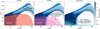 |
Fig. 5 Abundance of gas-phase H2O in a representative model for the HL Tau disk (colored background). The orange, pink, and cyan contours indicate the τdust = 1 surface for the lines in Table 3 in the mid-IR, far-IR, and (sub)millimeter, respectively. In the middle and right panels the solid and dashed lines indicate the long- and short-wavelength ends of the range of lines in Table 3, in the far-IR and (sub)millimeter, respectively. The water snow surface in the model is indicated with the black contour. |
4.4 H2O versus H13CO+
The radial profiles of the high-resolution H2O data suggest that the water snow line is located inside the inner beam of the observations. Another tracer of the water snow line is H13CO+, where ring-shaped emission is expected outside the water snow line as gas-phase water destroys HCO+ (Leemker et al. 2021). Other possible causes for a central hole in the H13CO+ emission include excitation, optically thick dust hiding the line emission, and absorption by the surrounding envelope. In this subsection we present the H13CO+ J = 2–1 line covered by the long-baseline ALMA data (Table 2). The integrated intensity map, the moment 1 map, and the spectrum are presented in Figs. A.7 and A.8.
The normalized azimuthally averaged radial profile of the H13CO+ emission in Fig. 6 shows that the emission is indeed ring-shaped and peaks at ∼80 au from the central star. Even though HL Tau is embedded in an envelope, no strong absorption feature is seen at the systemic velocity in the H2O and H13CO+ spectra (see Fig. A.4 and the right panel of Fig. A.8). Therefore, the effect of the envelope on the central hole in H13CO+ emission is at most marginal.
To investigate the effect of optically thick dust hiding the H13CO+ emission in the center, the H13CO+ J = 2–1 (173.507 GHz) radial profile is compared to that of the 13C17O J = 3–2 emission at 321.852 GHz presented in Booth & Ilee (2020). Under the assumption that the underlying 13C17O column density profile is independent of radius and the line is optically thin, the substructures seen in the 13C17O emission trace the effects of the optically thick dust.
Interestingly, the H13CO+ and 13C17O emission both exhibit a ring at roughly the same radius of ∼80 au, similar to the ring detected in H2CO, H2CS, and CS (Garufi et al. 2021). Inside this radius, both profiles decline, with H13CO+ continuing to decrease steadily toward the central star, while the 13C17O emission rises inward of the 40 au gap. Dust modeling of the HL Tau disk indicates that the continuum becomes optically thick inside ∼60 au for compact grains, or inside ∼115 au if the grains are ∼90% porous (Carrasco-González et al. 2019; Guerra-Alvarado et al. 2024; Ueda et al. 2025). As H13CO+, which is likely optically thin or close to optically thin, primarily emits from the dense disk midplane, the optically thick dust absorbs these line photons, producing the observed central hole (e.g., Bosman et al. 2021).
The contrasting morphology (H13CO+ showing a central cavity, and H2O and 13C17O exhibiting centrally peaked emission) can be explained by the disk’s 3D geometry and the interaction between line and continuum opacity. Line emission from higher disk layers can still escape if the molecule remains abundant above the dust τ = 1 surface. Isella et al. (2016) and Weaver et al. (2018) show that for an optically thick line, the intensity after continuum subtraction reflects the difference between gas and dust temperatures as the gas absorbs part of the continuum emission. Because the gas in the layers where H2O and 13C17O originate is warmer than the dust in the cooler midplane, line photons emitted from above the optically thick dust can still be observed as a central peak in azimuthally averaged radial profiles. The absence of a similar increase in the H13CO+ profile indicates that this line does not become optically thick above the τdust = 1 surface, despite model predictions that the HCO+ column density increases to several ×1013 cm−2 outside the water snow line (Leemker et al. 2021) and despite its lower frequency compared to the 13C17O transition.
In summary, the disk’s 3D structure hides emission from molecules located below the τdust = 1 surface (e.g., H13CO+) while still allowing photons from species abundant above this layer such as H2O and 13C17O to escape. Therefore, the central depression in H13CO+ is likely caused by optically thick dust rather than by the water snow line.
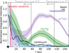 |
Fig. 6 Azimuthally averaged radial profiles of the H2O 183 GHz line imaged with robust = 0, the H13CO+ J = 2–1 line, the 13C17O J = 3–2 line from Booth & Ilee (2020), and the 1.7 mm continuum. The vertical gray lines indicate where the 1.3 mm continuum emission becomes optically thick assuming compact grains or grains with a 90% porosity (Guerra-Alvarado et al. 2024), and the upper limit on the water snow line location is indicated with the vertical red line. |
5 Discussion
5.1 Location of the water snow line in the HL tau disk
The midplane dust temperature derived from modeling high-resolution, multiwavelength continuum observations shows that the water snow line is located around 5 au in the disk midplane (Carrasco-González et al. 2019; Guerra-Alvarado et al. 2024; Ueda et al. 2025). The similarity in the location of the midplane water snow line derived from the dust and the upper limit of ∼6 au based on the H2O emission suggests that the water snow line is close to vertical up to the height where the H2O 183 GHz line becomes optically thick as the ALMA observations likely do not trace down to the disk midplane.
The diffuse H2O emission seen outside the central beam likely traces hot water at an excitation temperature of ∼350 K, consistent with that expected for the reformed water reservoir in the disk surface (T > 300 K). The presence of this reservoir is further supported by the highly excited H2O lines observed with Gemini North (Eu = 4945–5781 K). The line profiles of these transitions are consistent with emission up to at least 5 au where the drop off in the radial profile might be due to the water snow line (Salyk et al. 2019). Finally, the slight asymmetry toward the north or northeast seen in the H2O 183 GHz line emission at moderate spatial resolution could be due to projection effects of this elevated layer, a disk wind traced by H2O emission, or due to the infalling streamer impacting the HL Tau disk in the north.
5.2 H2O and SO
The HL Tau disk is impacted in the north by an infalling streamer seen in HCO+ (Yen et al. 2019; Gupta et al. 2024). The resulting shock releases energy into the disk, liberating SO and SO2 (Garufi et al. 2021). The lower limit of the excitation temperature of the SO2 in the HL Tau inner disk of >350 K is consistent with the excitation temperature of the H2O obtained from the radially resolved rotational diagram, suggesting a possible link between the water and the shock tracers SO and SO2.
In Fig. 7, we present a comparison of the velocity structure of the cold SO 44–33 transition (Eu = 33.7 K) covered by the long-baseline data and the H2O 183 GHz line. The SO shows compact emission on the scale of the disk (r ≲ 0′′.17) and extended emission to the southwest out to ∼2′′. The latter consists of two components: a streamer and a molecular outflow or wind (see also Fig. A.10). The streamer is indicated with the purple contour and overlaps with that seen in HCO+. The outflow or wind component is indicated with the orange contour and is similar to that seen in CO (Lumbreras & Zapata 2014; Bacciotti et al. 2025).
The velocity structure of the SO emission is compared to that of the water imaged with a robust parameter of 0.5 and 2.0 in the middle and right panels of Fig. 7. The high-resolution H2O map in the middle panel shows complex structures in the velocity. A velocity gradient is seen along the disk major axis indicating Keplerian rotation, similar to the SO emission in the inner 0′′.17. In the north, the H2O moment 1 map imaged with a small robust parameter of 0.5 shows some redshifted emission aligning with the redshifted emission seen in the SO streamer at that location. This hints that some of the H2O emission might be due to the shock impacting the disk. In addition, some redshifted H2O emission is seen in the south when imaged at moderate spatial resolution (robust = 2.0). As this image probes the diffuse water in the disk surface layers, the redshifted emission could indicate a connection to the outflow or a disk wind (Lumbreras & Zapata 2014; Bacciotti et al. 2025). All in all, the water shows a highly complex velocity structure with indications of Keplerian rotation in the center, and a possible connection to a streamer, molecular outflow or wind.
 |
Fig. 7 Moment 1 maps of the SO 44–33 transition (left) and the H2O 183 GHz line imaged with a robust parameter of 0.5 (middle) and 2.0 (right). The orange and purple contours indicate the emission above 5σ in the SO channel at 8 and 10 km s−1 tracing primarily the molecular outflow and the streamer, respectively, where 1σ corresponds to 0.3 mJy beam−1. The beam of the respective moment 1 maps is indicated in the bottom-left corner of each panel, and a 20 au scale bar is shown in the right panel. |
6 Conclusions
We have presented the first high-resolution images (∼0′′.08) of the H2O line at 183 GHz in the HL Tau disk. We derived the radially resolved temperature profile of the water emission through a rotational diagram analysis with the 321 GHz line of H2O. In addition, we quantified the fraction of the water reservoir visible at submillimeter wavelengths and compared this to that at far-and mid-IR wavelengths. Finally, H13CO+ emission was examined as a snow line tracer in this disk. In summary, we find that:
The H2O 183 GHz line shows a central, compact, and optically thick component and diffuse emission that extends out to ∼75 au. The emission in the central beam probes the water inside the water snow line at ≲6 au at the height probed by the observations. The disk midplane is hidden due to optical depth effects of the water and dust;
A disk-integrated rotational diagram comparing H2O lines seen at (sub)millimeter wavelengths to those at far- and mid-IR wavelengths demonstrates that the lines seen with ALMA probe a 2–3 order of magnitude higher column density of water. This is primarily due to optically thick dust hiding 98–99.98% of the water reservoir at far-and mid-IR wavelengths;
Correcting the disk-integrated rotational diagram for optically thick dust shows that the H2O 183, 321, and 325 GHz lines are not strongly masing;
Observing the H2O 183 GHz line directly is a better probe of the water snow line than the H13CO+ J = 2–1 line due to the presence of optically thick dust;
Some of the H2O emission might originate due to the infalling streamer impacting the disk, which, for the first time, was detected in SO. This cold SO 44–33 transition traces the disk, the infalling streamer seen in HCO+, and the molecular outflow (Lumbreras & Zapata 2014; Yen et al. 2019; Bacciotti et al. 2025).
This work demonstrates that observing the H2O 183 GHz line at high spatial resolution is the most effective strategy for directly tracing the water snow line in disks. Other tracers such as H13CO+ and CH3OH emission are affected by optically thick dust and/or not detected in this disk (Soave et al. submitted). Similarly, water lines in the mid- and far-IR regime trace the water snow line in the disk surface layers due to the high-continuum optical depth. Instead, the 183 GHz line probes much closer to the disk midplane, providing the best strategy for deriving the water snow line.
Acknowledgements
We thank the referee Shigehisa Takakuwa for the constructive comments. M.L. acknowledges assistance from Allegro, the European ALMA Regional Center node in The Netherlands. M.L., S.F., and L.R. are funded by the European Union (ERC, UNVEIL, 101076613). Views and opinions expressed are however those of the author(s) only and do not necessarily reflect those of the European Union or the European Research Council. Neither the European Union nor the granting authority can be held responsible for them. S.F. acknowledges financial contribution from PRIN-MUR 2022YP5ACE. P.C. acknowledges support by the ANID BASAL project FB210003. M.B. has received funding from the European Research Council (ERC) under the European Union’s Horizon 2020 research and innovation programme (PRO-TOPLANETS, grant agreement No. 101002188). This paper makes use of the following ALMA data: ADS/JAO.ALMA#2017.1.01178.S, #2017.1.01562.S, #2021.1.01310.S, and #2022.1.00905.S. ALMA is a partnership of ESO (representing its member states), NSF (USA) and NINS (Japan), together with NRC (Canada), NSTC and ASIAA (Taiwan), and KASI (Republic of Korea), in cooperation with the Republic of Chile. The Joint ALMA Observatory is operated by ESO, AUI/NRAO and NAOJ.
References
- ALMA Partnership (Brogan, C. L., et al.) 2015, ApJ, 808, L3 [Google Scholar]
- Alonso-Martínez, M., Riviere-Marichalar, P., Meeus, G., et al. 2017, A&A, 603, A138 [EDP Sciences] [Google Scholar]
- Andrews, S. M., Huang, J., Pérez, L. M., et al. 2018, ApJ, 869, L41 [NASA ADS] [CrossRef] [Google Scholar]
- Bacciotti, F., Nony, T., Podio, L., et al. 2025, A&A, 704, A157 [NASA ADS] [CrossRef] [EDP Sciences] [Google Scholar]
- Banzatti, A., Pontoppidan, K. M., Carr, J. S., et al. 2023, ApJ, 957, L22 [NASA ADS] [CrossRef] [Google Scholar]
- Banzatti, A., Salyk, C., Pontoppidan, K. M., et al. 2025, AJ, 169, 165 [Google Scholar]
- Barber, R. J., Tennyson, J., Harris, G. J., & Tolchenov, R. N. 2006, MNRAS, 368, 1087 [Google Scholar]
- Beck, T. L., Bary, J. S., & McGregor, P. J. 2010, ApJ, 722, 1360 [NASA ADS] [CrossRef] [Google Scholar]
- Bergin, E. A., Melnick, G. J., & Neufeld, D. A. 1998, ApJ, 499, 777 [Google Scholar]
- Booth, A. S., & Ilee, J. D. 2020, MNRAS, 493, L108 [NASA ADS] [CrossRef] [Google Scholar]
- Bosman, A. D., & Bergin, E. A. 2021, ApJ, 918, L10 [NASA ADS] [CrossRef] [Google Scholar]
- Bosman, A. D., Bergin, E. A., Loomis, R. A., et al. 2021, ApJS, 257, 15 [NASA ADS] [CrossRef] [Google Scholar]
- Bosman, A. D., Bergin, E. A., Calahan, J., & Duval, S. E. 2022, ApJ, 930, L26 [NASA ADS] [CrossRef] [Google Scholar]
- Briceño, C., Luhman, K. L., Hartmann, L., Stauffer, J. R., & Kirkpatrick, J. D. 2002, ApJ, 580, 317 [NASA ADS] [CrossRef] [Google Scholar]
- Bruderer, S. 2013, A&A, 559, A46 [NASA ADS] [CrossRef] [EDP Sciences] [Google Scholar]
- Bruderer, S., Doty, S. D., & Benz, A. O. 2009, ApJS, 183, 179 [Google Scholar]
- Bruderer, S., van Dishoeck, E. F., Doty, S. D., & Herczeg, G. J. 2012, A&A, 541, A91 [NASA ADS] [CrossRef] [EDP Sciences] [Google Scholar]
- Carr, J. S., Najita, J. R., & Salyk, C. 2018, RNAAS, 2, 169 [Google Scholar]
- Carrasco-González, C., Sierra, A., Flock, M., et al. 2019, ApJ, 883, 71 [Google Scholar]
- CASA Team (Bean, B., et al.) 2022, PASP, 134, 114501 [NASA ADS] [CrossRef] [Google Scholar]
- Casassus, S., & Cárcamo, M. 2022, MNRAS, 513, 5790 [NASA ADS] [CrossRef] [Google Scholar]
- Cheng, Y. C., Bockelée-Morvan, D., Roos-Serote, M., et al. 2022, A&A, 663, A43 [NASA ADS] [CrossRef] [EDP Sciences] [Google Scholar]
- Comrie, A., Wang, K.-S., Hwang, Y.-H., et al. 2024, https://doi.org/10.5281/zenodo.15172686 [Google Scholar]
- Czekala, I., Loomis, R. A., Teague, R., et al. 2021, ApJS, 257, 2 [NASA ADS] [CrossRef] [Google Scholar]
- Drążkowska, J., & Alibert, Y. 2017, A&A, 608, A92 [Google Scholar]
- Facchini, S., Testi, L., Humphreys, E., et al. 2024, Nat. Astron., 8, 587 [Google Scholar]
- Fasano, D., Benisty, M., Curone, P., et al. 2025, A&A, 699, A373 [NASA ADS] [CrossRef] [EDP Sciences] [Google Scholar]
- Faure, A., & Josselin, E. 2008, A&A, 492, 257 [NASA ADS] [CrossRef] [EDP Sciences] [Google Scholar]
- Furlan, E., McClure, M., Calvet, N., et al. 2008, ApJS, 176, 184 [NASA ADS] [CrossRef] [Google Scholar]
- Galli, P. A. B., Loinard, L., Ortiz-Léon, G. N., et al. 2018, ApJ, 859, 33 [Google Scholar]
- Garufi, A., Podio, L., Codella, C., et al. 2021, A&A, 645, A145 [EDP Sciences] [Google Scholar]
- Garufi, A., Podio, L., Codella, C., et al. 2022, A&A, 658, A104 [CrossRef] [EDP Sciences] [Google Scholar]
- Gasman, D., van Dishoeck, E. F., Grant, S. L., et al. 2023, A&A, 679, A117 [NASA ADS] [CrossRef] [EDP Sciences] [Google Scholar]
- Goldsmith, P. F., & Langer, W. D. 1999, ApJ, 517, 209 [Google Scholar]
- Gray, M. D., Baudry, A., Richards, A. M. S., et al. 2016, MNRAS, 456, 374 [NASA ADS] [CrossRef] [Google Scholar]
- Guerra-Alvarado, O. M., Carrasco-González, C., Macías, E., et al. 2024, A&A, 686, A298 [NASA ADS] [CrossRef] [EDP Sciences] [Google Scholar]
- Gupta, A., Miotello, A., Williams, J. P., et al. 2024, A&A, 683, A133 [NASA ADS] [CrossRef] [EDP Sciences] [Google Scholar]
- Harsono, D., Bruderer, S., & van Dishoeck, E. F. 2015, A&A, 582, A41 [NASA ADS] [CrossRef] [EDP Sciences] [Google Scholar]
- Hartmann, L., Calvet, N., Gullbring, E., & D’Alessio, P. 1998, ApJ, 495, 385 [NASA ADS] [CrossRef] [Google Scholar]
- Houge, A., Krijt, S., Banzatti, A., et al. 2025, MNRAS, 537, 691 [CrossRef] [Google Scholar]
- Isella, A., Guidi, G., Testi, L., et al. 2016, Phys. Rev. Lett., 117, 251101 [NASA ADS] [CrossRef] [Google Scholar]
- Jorsater, S., & van Moorsel, G. A. 1995, AJ, 110, 2037 [Google Scholar]
- Kaeufer, T., Min, M., Woitke, P., Kamp, I., & Arabhavi, A. M. 2024, A&A, 687, A209 [NASA ADS] [CrossRef] [EDP Sciences] [Google Scholar]
- Kristensen, L. E., Brown, J. M., Wilner, D., & Salyk, C. 2016, ApJ, 822, L20 [Google Scholar]
- Leemker, M., van’t Hoff, M. L. R., Trapman, L., et al. 2021, A&A, 646, A3 [EDP Sciences] [Google Scholar]
- Leemker, M., Booth, A. S., van Dishoeck, E. F., et al. 2022, A&A, 663, A23 [NASA ADS] [CrossRef] [EDP Sciences] [Google Scholar]
- Leemker, M., Booth, A. S., van Dishoeck, E. F., et al. 2023, A&A, 673, A7 [NASA ADS] [CrossRef] [EDP Sciences] [Google Scholar]
- Liu, Y., Henning, T., Carrasco-González, C., et al. 2017, A&A, 607, A74 [NASA ADS] [CrossRef] [EDP Sciences] [Google Scholar]
- Loomis, R. A., Cleeves, L. I., Öberg, K. I., et al. 2018, ApJ, 859, 131 [Google Scholar]
- Loomis, R. A., Facchini, S., Benisty, M., et al. 2025, ApJ, 984, L7 [Google Scholar]
- Lumbreras, A. M., & Zapata, L. A. 2014, AJ, 147, 72 [NASA ADS] [CrossRef] [Google Scholar]
- Lynden-Bell, D., & Pringle, J. E. 1974, MNRAS, 168, 603 [Google Scholar]
- McMullin, J. P., Waters, B., Schiebel, D., Young, W., & Golap, K. 2007, in Astronomical Society of the Pacific Conference Series, 376, Astronomical Data Analysis Software and Systems XVI, eds. R. A. Shaw, F. Hill, & D. J. Bell, 127 [Google Scholar]
- Milam, S. N., Savage, C., Brewster, M. A., Ziurys, L. M., & Wyckoff, S. 2005, ApJ, 634, 1126 [Google Scholar]
- Miotello, A., van Dishoeck, E. F., Kama, M., & Bruderer, S. 2016, A&A, 594, A85 [NASA ADS] [CrossRef] [EDP Sciences] [Google Scholar]
- Öberg, K. I., & Bergin, E. A. 2021, Phys. Rep., 893, 1 [Google Scholar]
- Öberg, K. I., Murray-Clay, R., & Bergin, E. A. 2011, ApJ, 743, L16 [Google Scholar]
- Phillips, T. G., van Dishoeck, E. F., & Keene, J. 1992, ApJ, 399, 533 [NASA ADS] [CrossRef] [Google Scholar]
- Pickett, H. M., Poynter, R. L., Cohen, E. A., et al. 1998, J. Quant. Spec. Radiat. Transf., 60, 883 [Google Scholar]
- Pinte, C., Dent, W. R. F., Ménard, F., et al. 2016, ApJ, 816, 25 [Google Scholar]
- Pirovano, L. M., Fedele, D., van Dishoeck, E. F., et al. 2022, A&A, 665, A45 [NASA ADS] [CrossRef] [EDP Sciences] [Google Scholar]
- Pontoppidan, K. M., Salyk, C., Blake, G. A., & Käufl, H. U. 2010, ApJ, 722, L173 [NASA ADS] [CrossRef] [Google Scholar]
- Pontoppidan, K. M., Salyk, C., Banzatti, A., et al. 2024, ApJ, 963, 158 [NASA ADS] [CrossRef] [Google Scholar]
- Rampinelli, L., Facchini, S., Leemker, M., et al. 2026, ApJ, 996, L17 [Google Scholar]
- Rebull, L. M., Wolff, S. C., & Strom, S. E. 2004, AJ, 127, 1029 [Google Scholar]
- Riviere-Marichalar, P., Ménard, F., Thi, W. F., et al. 2012, A&A, 538, L3 [NASA ADS] [CrossRef] [EDP Sciences] [Google Scholar]
- Robitaille, T. P., Whitney, B. A., Indebetouw, R., & Wood, K. 2007, ApJS, 169, 328 [Google Scholar]
- Salyk, C., Lacy, J., Richter, M., et al. 2019, ApJ, 874, 24 [NASA ADS] [CrossRef] [Google Scholar]
- Schöier, F. L., van der Tak, F. F. S., van Dishoeck, E. F., & Black, J. H. 2005, A&A, 432, 369 [Google Scholar]
- Schoonenberg, D., & Ormel, C. W. 2017, A&A, 602, A21 [NASA ADS] [CrossRef] [EDP Sciences] [Google Scholar]
- Skinner, S. L., & Güdel, M. 2020, ApJ, 888, 15 [NASA ADS] [CrossRef] [Google Scholar]
- Teague, R. 2019, J. Open Source Softw., 4, 1632 [NASA ADS] [CrossRef] [Google Scholar]
- Temmink, M., van Dishoeck, E. F., Gasman, D., et al. 2024, A&A, 689, A330 [NASA ADS] [CrossRef] [EDP Sciences] [Google Scholar]
- Tennyson, J., Zobov, N. F., Williamson, R., Polyansky, O. L., & Bernath, P. F. 2001, J. Phys. Chem. Ref. Data, 30, 735 [NASA ADS] [CrossRef] [Google Scholar]
- Tobin, J. J., van’t Hoff, M. L. R., Leemker, M., et al. 2023, Nature, 615, 227 [NASA ADS] [CrossRef] [Google Scholar]
- Ueda, T., Andrews, S. M., Carrasco-González, C., et al. 2025, ApJ, 990, 183 [Google Scholar]
- van Dishoeck, E. F., Kristensen, L. E., Mottram, J. C., et al. 2021, A&A, 648, A24 [NASA ADS] [CrossRef] [EDP Sciences] [Google Scholar]
- van ’t Hoff, M. L. R., Tobin, J. J., Trapman, L., et al. 2018, ApJ, 864, L23 [Google Scholar]
- Vlasblom, M., Temmink, M., Sellek, A. D., & van Dishoeck, E. F. 2025, A&A, 703, A52 [NASA ADS] [CrossRef] [EDP Sciences] [Google Scholar]
- Wang, Y., Ormel, C. W., Mori, S., & Bai, X.-N. 2025, A&A, 696, A38 [NASA ADS] [CrossRef] [EDP Sciences] [Google Scholar]
- Weaver, E., Isella, A., & Boehler, Y. 2018, ApJ, 853, 113 [Google Scholar]
- Wilson, T. L. 1999, Rep. Prog. Phys., 62, 143 [Google Scholar]
- Yang, H., Stephens, I. W., Lin, Z.-Y. D., et al. 2025, ApJ, 989, L43 [Google Scholar]
- Yen, H.-W., Gu, P.-G., Hirano, N., et al. 2019, ApJ, 880, 69 [NASA ADS] [CrossRef] [Google Scholar]
- Yu, S., Pearson, J. C., Drouin, B. J., et al. 2012, J. Mol. Spectrosc., 279, 16 [NASA ADS] [CrossRef] [Google Scholar]
Appendix A Observations
A.1 Frequency-dependent noise in the H2O 183 GHz spectra
The H2O 183 GHz line has an upper energy level of 205 K, comparable to the temperature of the water in some layers of the Earth’s atmosphere. Therefore, this line is by definition located in a strong telluric. The effect of this telluric on the noise in the spw covering the 183 GHz H2O line is demonstrated in Fig. A.1, where the left panel presents the spectra as a function of the topocentric velocity where the telluric is at 0 km s−1 and the right panel presents those in the local standard of rest frame. Each spectrum corresponds to one EB of data taken during the short- or long-baseline EBs in Table 1. The spectra are extracted from the cubes imaged with a robust parameter of 0.0 from a 7" square region excluding the inner 1"×0′′.7 elliptical region where the continuum is seen using CARTA (Comrie et al. 2024). The noise in the short-baseline data (purple) is extremely low due to the exceptional weather conditions, with only 0.2 mm of precipitable water vapor (pwv) during the observations, whereas that in each of the seven long-baseline EBs is higher due to the larger pwv of 0.4–0.5 mm (see Table 1). In addition, the velocity where the noise is largest is always at 0 km s−1 in topocentric units but it shifts in the kinematic local standard of rest (LSRK) frame as the conversion between the two frames depends on, for example, the time and date of the observations. Therefore, the channel rms in the combined image is elevated over a larger velocity range than in the individual EBs.
The varying weather conditions across the EBs not only affect the rms in the spectra, but they also affect the bandwidth over which the data are averaged for the bandpass calibration as part of the automated ALMA data reduction pipeline. The EBs where this bandwidth was small (≲ 2 km s−1) show a narrow peak of a few km s−1 in the rms spectra due to the tel-luric whereas those binned over a larger velocity range up to 9.6 km s−1 show a much wider peak where the noise is elevated. All in all, the resulting noise spectrum is complex with frequency-dependent noise depending on, for example, the time between different EBs and under which weather conditions the data were taken.
A.2 Channel maps, moment maps, and spectra
The channel maps of the H2O 183 GHz line imaged at two different spatial resolutions are presented in Figs. A.2 and A.3. The 3σ and 5σ contours in both figures are computed using the rms noise in each channel separately following Appendix A.1. The corresponding spectra extracted from a small 0′′.28 and larger 0′′.7 region are presented in Fig. A.4. The azimuthally averaged radial profile of the H2O 183 GHz line imaged with a larger robust parameters of 0.0 up to 2.0 are presented in Fig. A.5. All radial profiles are JvM-corrected to correct for the non-Gaussian shape of the beam affecting the diffuse, large-scale emission. The H2O emission shows a bright inner component and shelf of diffuse emission extending out to ∼75 au that is only detected when imaged with a larger beam size than the robust = 0 image.
The H13CO+ J = 2 − 1 channel maps are presented in Fig. A.6. The integrated intensity and the moment 1 and 8 maps of the H13CO+ emission are presented in Fig. A.7, where the moment 8 map is converted to brightness temperature using the Rayleigh-Jeans approximation. Even though the line is weak, a ring shaped profile is clearly visible when applying a Keplerian mask to the data before creating the integrated intensity map and in the moment 1 and 8 map without any masking applied. In addition, the moment 1 map shows a velocity gradient along the disk major axis, consistent with what is expected from a Keple-rian rotating disk. Finally, the H13CO+ spectrum extracted from a 1′′.2 × 0′′.8 region is presented in the left panel of Fig. A.8. The middle panel represents the spatially integrated spectrum extracted after shifting each pixel by the local projected Keple-rian velocity in the disk. This effectively removes the Doppler line broadening from the spectrum due to the Keplerian rotation, decreasing the linewidth and increasing the signal-to-noise ratio in the spectrum. The middle panel clearly shows that the H13CO+ emission is detected at the expected velocity. The right panel shows the H13CO+ spectrum extracted from a small elliptical region without shifting and stacking. No strong absorption is detected at the systemic velocity in the disk center, indicating that the hole seen in the H13CO+ moment maps is not primarily due to absorption of emission in the envelope.
The channel maps, integrated intensity maps, and the spectrum of the SO emission are presented in Figs. A.9 and A.10. The left panel of the latter figure shows a zoom in of the disk and the middle panel shows the map integrated over a narrower velocity range of 5 to 13 km s−1 instead of -5 to 19 km s−1 to highlight the SO streamer and molecular outflow. Additionally, the SO spectrum is presented in the right panel.
Appendix B Thermochemical model
To investigate the fraction of the water reservoir accessible to observations at various wavelengths, we constructed a simple thermochemical model reproducing the rare CO isotopologue lines seen with ALMA and the 0.95 mm continuum emission within a factor of 2 in most disk regions. We focused on the C18O, 13C18O, and 13C17O J = 3 − 2 lines seen with ALMA to trace the HL Tau disk and minimize the effect of the surrounding envelope and molecular outflow seen in, for example, CO (Furlan et al. 2008; Lumbreras & Zapata 2014; Bacciotti et al. 2025).
The disk is modeled using the thermo-chemical modeling code DALI (Bruderer et al. 2009, 2012; Bruderer 2013). We used the standard model for a full disk that is described by parameters for a viscously evolving disk between 0.23 and 500 au (Lynden-Bell & Pringle 1974; Hartmann et al. 1998):
![Mathematical equation: ${\Sigma _{{\rm{gas}}}} = {\Sigma _c}{\left( {{r \over {{r_c}}}} \right)^{ - \gamma }}\exp \left[ { - {{\left( {{r \over {{r_c}}}} \right)}^{2 - \gamma }}} \right],$](/articles/aa/full_html/2026/01/aa57609-25/aa57609-25-eq17.png) (B.1)
(B.1)
with Σc setting the surface density at the characteristic radius rc and γ = 1 the power law index of the profile. We set the total disk mass to 0.2 M⊙ based on the 13C17O detection in this disk (Booth & Ilee 2020) and the characteristic radius to 30 au to roughly match the morphology of the CO isotopologue emission. The disk scale height hc is set to 0.1 (Pinte et al. 2016), whereas the grains are settled to the disk midplane with a scale height of 0.05 × hc as the dust disk is generally flat (Guerra-Alvarado et al. 2024; Yang et al. 2025). The disk flaring is parametrized as h = hc(r/rc)ψ, with a flaring index of 0.15.
The stellar spectrum is modeled as a 4000 K black body (Liu et al. 2017), where the mass accretion rate of 8.7 × 10⁻⁸ M⊙ yr−1 is modeled as an additional 10000 K black body spectrum (Beck et al. 2010). The X-ray luminosity of the star is 3.36×1030 erg s−1 (Skinner & Güdel 2020) and a cosmic ray ionization rate of 10−17 s−1 is assumed. The stellar mass is set to 2.1 M⊙ (Yen et al. 2019).
Initially the model is run time independently with a small chemical network consisting of 109 species and 1463 reactions. This network is sufficient to obtain the temperature structure of the disk and includes the H2O self-shielding (Bosman et al. 2022). Then the model is either run with the same network time dependently for 1 Myr, the approximate age of the disk (Briceño et al. 2002), to obtain the water abundance or it is run time-dependently with the CO isotopologue network described in Miotello et al. (2016) to model the emission of the CO isotopologues.
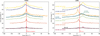 |
Fig. A.1 RMS as a function of frequency in the spws covering the H2O 183 GHz line imaged with a robust parameter of 0.0. Left: Spectra in topocentric coordinates. The telluric due to the water in the Earth’s atmosphere increases the noise at a velocity of 0 km s−1. Right: Same spectra but in the local standard of rest frame. The number within brackets in the labels indicates the velocity width used for the bandpass calibration. |
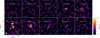 |
Fig. A.2 Channel maps of the H2O line at 183 GHz imaged with a robust parameter of 0.0. The white contours indicate the 3σ and 5σ confidence levels, where 1σ corresponds to 1.5-1.7 mJy beam−1 depending on the velocity channel (see Appendix A.1). The beam and a 20 au scale bar are indicated in the bottom-left panel. |
The CO isotopologue network is suited to model the emission of rare CO isotopologues as isotope selective effects of single CO isotopologues are taken into account, as is the self-shielding of the individual isotopologues. Mutual self-shielding is not included. This network uses a 12C/13C ratio of 70, a 16O/18O ratio of 560, and a 18O/17O ratio of 3.6 (Wilson 1999; Milam et al. 2005).
Figure B.1 presents the resulting azimuthally averaged radial profiles of the C18O, 13C18O, and 13C17O J = 3 − 2 emission predicted by the CO isotopologue network and the 0.95 mm continuum emission. These profiles are compared to the observed profiles from Booth & Ilee (2020) and the product data from ALMA program 2021.1.01310.S (PI: K. Zhang) that will be presented in detail in TorresVillanueva et al. (in preparation). The modeled radial profiles reproduce the data within a factor of < 2 for most disk radii at the resolution of the data.
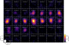 |
Fig. A.3 Channel maps of the H2O line at 183 GHz imaged with a robust parameter of 2.0. The white contours indicate the 3σ and 5σ confidence intervals, where 1σ corresponds to 5-7 mJy beam−1 depending on the velocity channel (see Appendix A.1). The beam and a 20 au scale bar are indicated in the bottom-left panel. |
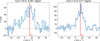 |
Fig. A.4 Spectra of the H2O emission extracted from the same regions used to calculate the disk-integrated flux without shifting and stacking the data. Left: Spectrum of the line imaged with a robust parameter of 0.0. Right: Spectrum when imaging with a robust parameter of 2.0. The source velocity of the HL Tau system is indicated by the vertical red line. |
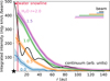 |
Fig. A.5 Azimuthally averaged radial profiles of the H2O line at 183 GHz imaged with a robust parameter of 0 (blue), 0.5 (orange), 1 (green), 1.5 (purple), and 2.0 (pink), all corrected for the non-Gaussian beam shape, and the continuum emission (black). The continuum emission is presented in arbitrary units. The upper limit on the water snow line location is indicated with the vertical red line. The beams are indicated with the horizontal bars in the top-right corner. |
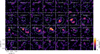 |
Fig. A.6 Channel maps of the H13CO+ J = 2 − 1 transition. The blue contours indicate the Keplerian mask used for the azimuthally averaged radial profile, and the white contours indicate the 3σ and 5σ confidence levels; 1σ corresponds to 0.7 mJy beam−1. |
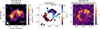 |
Fig. A.7 Moment 0 (left), 1 (middle), and 8 (right) maps of the H13CO+ emission in the HL Tau disk. A Keplerian mask was applied to the data before making the moment 0 map but not before making the moment 1 and 8 maps. |
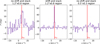 |
Fig. A.8 Spectrum of the H13CO+ J = 2 − 1 line extracted from a 1′′.2 × 0′′.8 elliptical region and an 0′′.5×0′′.3 elliptical region positioned in the hole seen in the H13CO+ moment maps. Left and right: Spectrum without shifting or stacking. Middle: Spectrum with shifting and stacking; each pixel is shifted by the projected Keplerian velocity at that location in the disk. The middle panel shows that the line is detected at the expected velocity. |
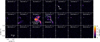 |
Fig. A.9 Channel maps of the SO 44 − 33 line. The channels at 8 and 10 km s−1 primarily trace the molecular outflow and the streamer, respectively. The green line in the 10 km s−1 channel is the fit to the one-arm spiral tracing the streamer in HCO+ (Yen et al. 2019). The white contours indicate the 3σ and 5σ confidence levels, where 1σ corresponds to 0.3 mJy beam−1. We note that the position of the disk is off center with respect to the center of the channel maps. |
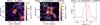 |
Fig. A.10 SO emission in the HL Tau system. Left and middle: Integrated intensity maps of the SO emission. The left panel presents the map integrated from -5 to 19 km s−1 zoomed in on the HL Tau disk, and the middle panel shows the emission integrated over a smaller velocity range from 5 to 13 km s−1, highlighting the emission coming from primarily the streamer (white) and the molecular outflow (orange contour). The green line in the middle panel is the fit to the one-arm spiral tracing the streamer in HCO+ (Yen et al. 2019). Right: SO spectrum. |
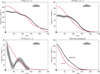 |
Fig. B.1 Azimuthally averaged radial profiles of the C18O, 13C18O, and 13C17O J = 3 − 2 transition in the HL Tau disk together with the 0.95 mm continuum. The data are shown in black and are taken from Booth & Ilee (2020) and the product data from ALMA project 2021.1.01310.S (PI: K. Zhang). The model predictions are shown in red. |
All Tables
All Figures
|
Fig. 1 ALMA Band 5 images of the HL Tau disk and the 321 GHz H2O line. Top left: continuum. Right panels: JvM-corrected integrated intensity maps of the H2O line at 183 GHz imaged with r = 0.0 (top) and r = 2.0 (bottom). These maps provide high and moderate spatial resolution. Top-right inset: zoomed-in view of the inner 0′′.2. This highlights the approximate water snow line location derived by Guerra-Alvarado et al. (2024) Bottom left: reimaged H2O 321 GHz line originally presented in Facchini et al. (2024). The beams are indicated in the bottom-left corners of the respective panels. The dust rings and gaps derived from high-resolution ALMA observations are indicated with solid and dashed arcs in each panel (ALMA Partnership 2015; Carrasco-González et al. 2019; Guerra-Alvarado et al. 2024), and a 20 au scale bar is shown in the bottom-right corner of the bottom-right panel. |
| In the text | |
|
Fig. 2 Azimuthally averaged radial profiles of the integrated intensity (left) and brightness temperature (right). The H2O line at 183 GHz imaged with a robust parameter of 0.0 is indicated in blue, the H2O line at 321 GHz in orange, and the continuum emission in black. In the left panel the continuum emission is presented in arbitrary units, and the upper limit on the water snow line location is indicated with the vertical red line. Note the difference in the radial axes. The beams are indicated with the horizontal bars in the top-right corner. |
| In the text | |
|
Fig. 3 Radially resolved rotational diagram analysis of the H2O emission in the HL Tau disk. The excitation temperature (left), column density (middle), and optical depth (right) of the H2O 183 GHz (blue) and 321 GHz (orange) lines are obtained after convolving the two lines to the same beam size. The dashed lines are derived under the assumption of fully optically thin emission, whereas the solid lines include the correction for the optical depth of the lines. The black scatter points indicate the disk-averaged results from Facchini et al. (2024) assuming an emitting region of 17 au; the upper limit on the water snow line location is indicated with the vertical red line. |
| In the text | |
|
Fig. 4 Rotational diagram summarizing the disk-integrated H2O line detections in the HL Tau disk with ALMA in the (sub)millimeter (cyan), Herschel PACS in the far-IR (pink), and Gemini North in the mid-IR (orange). Left: rotational diagram without a correction for the difference in the continuum optical depth for the various lines. Right: rotational diagram with a correction factor derived from a thermochemical model. The shaded points in the right panel are identical to the non-shaded points in the left panel. |
| In the text | |
|
Fig. 5 Abundance of gas-phase H2O in a representative model for the HL Tau disk (colored background). The orange, pink, and cyan contours indicate the τdust = 1 surface for the lines in Table 3 in the mid-IR, far-IR, and (sub)millimeter, respectively. In the middle and right panels the solid and dashed lines indicate the long- and short-wavelength ends of the range of lines in Table 3, in the far-IR and (sub)millimeter, respectively. The water snow surface in the model is indicated with the black contour. |
| In the text | |
|
Fig. 6 Azimuthally averaged radial profiles of the H2O 183 GHz line imaged with robust = 0, the H13CO+ J = 2–1 line, the 13C17O J = 3–2 line from Booth & Ilee (2020), and the 1.7 mm continuum. The vertical gray lines indicate where the 1.3 mm continuum emission becomes optically thick assuming compact grains or grains with a 90% porosity (Guerra-Alvarado et al. 2024), and the upper limit on the water snow line location is indicated with the vertical red line. |
| In the text | |
|
Fig. 7 Moment 1 maps of the SO 44–33 transition (left) and the H2O 183 GHz line imaged with a robust parameter of 0.5 (middle) and 2.0 (right). The orange and purple contours indicate the emission above 5σ in the SO channel at 8 and 10 km s−1 tracing primarily the molecular outflow and the streamer, respectively, where 1σ corresponds to 0.3 mJy beam−1. The beam of the respective moment 1 maps is indicated in the bottom-left corner of each panel, and a 20 au scale bar is shown in the right panel. |
| In the text | |
|
Fig. A.1 RMS as a function of frequency in the spws covering the H2O 183 GHz line imaged with a robust parameter of 0.0. Left: Spectra in topocentric coordinates. The telluric due to the water in the Earth’s atmosphere increases the noise at a velocity of 0 km s−1. Right: Same spectra but in the local standard of rest frame. The number within brackets in the labels indicates the velocity width used for the bandpass calibration. |
| In the text | |
|
Fig. A.2 Channel maps of the H2O line at 183 GHz imaged with a robust parameter of 0.0. The white contours indicate the 3σ and 5σ confidence levels, where 1σ corresponds to 1.5-1.7 mJy beam−1 depending on the velocity channel (see Appendix A.1). The beam and a 20 au scale bar are indicated in the bottom-left panel. |
| In the text | |
|
Fig. A.3 Channel maps of the H2O line at 183 GHz imaged with a robust parameter of 2.0. The white contours indicate the 3σ and 5σ confidence intervals, where 1σ corresponds to 5-7 mJy beam−1 depending on the velocity channel (see Appendix A.1). The beam and a 20 au scale bar are indicated in the bottom-left panel. |
| In the text | |
|
Fig. A.4 Spectra of the H2O emission extracted from the same regions used to calculate the disk-integrated flux without shifting and stacking the data. Left: Spectrum of the line imaged with a robust parameter of 0.0. Right: Spectrum when imaging with a robust parameter of 2.0. The source velocity of the HL Tau system is indicated by the vertical red line. |
| In the text | |
|
Fig. A.5 Azimuthally averaged radial profiles of the H2O line at 183 GHz imaged with a robust parameter of 0 (blue), 0.5 (orange), 1 (green), 1.5 (purple), and 2.0 (pink), all corrected for the non-Gaussian beam shape, and the continuum emission (black). The continuum emission is presented in arbitrary units. The upper limit on the water snow line location is indicated with the vertical red line. The beams are indicated with the horizontal bars in the top-right corner. |
| In the text | |
|
Fig. A.6 Channel maps of the H13CO+ J = 2 − 1 transition. The blue contours indicate the Keplerian mask used for the azimuthally averaged radial profile, and the white contours indicate the 3σ and 5σ confidence levels; 1σ corresponds to 0.7 mJy beam−1. |
| In the text | |
|
Fig. A.7 Moment 0 (left), 1 (middle), and 8 (right) maps of the H13CO+ emission in the HL Tau disk. A Keplerian mask was applied to the data before making the moment 0 map but not before making the moment 1 and 8 maps. |
| In the text | |
|
Fig. A.8 Spectrum of the H13CO+ J = 2 − 1 line extracted from a 1′′.2 × 0′′.8 elliptical region and an 0′′.5×0′′.3 elliptical region positioned in the hole seen in the H13CO+ moment maps. Left and right: Spectrum without shifting or stacking. Middle: Spectrum with shifting and stacking; each pixel is shifted by the projected Keplerian velocity at that location in the disk. The middle panel shows that the line is detected at the expected velocity. |
| In the text | |
|
Fig. A.9 Channel maps of the SO 44 − 33 line. The channels at 8 and 10 km s−1 primarily trace the molecular outflow and the streamer, respectively. The green line in the 10 km s−1 channel is the fit to the one-arm spiral tracing the streamer in HCO+ (Yen et al. 2019). The white contours indicate the 3σ and 5σ confidence levels, where 1σ corresponds to 0.3 mJy beam−1. We note that the position of the disk is off center with respect to the center of the channel maps. |
| In the text | |
|
Fig. A.10 SO emission in the HL Tau system. Left and middle: Integrated intensity maps of the SO emission. The left panel presents the map integrated from -5 to 19 km s−1 zoomed in on the HL Tau disk, and the middle panel shows the emission integrated over a smaller velocity range from 5 to 13 km s−1, highlighting the emission coming from primarily the streamer (white) and the molecular outflow (orange contour). The green line in the middle panel is the fit to the one-arm spiral tracing the streamer in HCO+ (Yen et al. 2019). Right: SO spectrum. |
| In the text | |
|
Fig. B.1 Azimuthally averaged radial profiles of the C18O, 13C18O, and 13C17O J = 3 − 2 transition in the HL Tau disk together with the 0.95 mm continuum. The data are shown in black and are taken from Booth & Ilee (2020) and the product data from ALMA project 2021.1.01310.S (PI: K. Zhang). The model predictions are shown in red. |
| In the text | |
Current usage metrics show cumulative count of Article Views (full-text article views including HTML views, PDF and ePub downloads, according to the available data) and Abstracts Views on Vision4Press platform.
Data correspond to usage on the plateform after 2015. The current usage metrics is available 48-96 hours after online publication and is updated daily on week days.
Initial download of the metrics may take a while.