| Issue |
A&A
Volume 706, February 2026
|
|
|---|---|---|
| Article Number | A55 | |
| Number of page(s) | 24 | |
| Section | Extragalactic astronomy | |
| DOI | https://doi.org/10.1051/0004-6361/202554407 | |
| Published online | 29 January 2026 | |
The HST-Hyperion Survey: Companion fraction and overdensity in a z ∼ 2.5 proto-supercluster
1
Institute for Astronomy, University of Hawai‘i 2680 Woodlawn Drive Honolulu HI 96822, USA
2
Gemini Observatory, NSF NOIRLab 670 N Aohoku Pl Hilo HI 96720, USA
3
Department of Physics and Astronomy, University of California, Davis One Shields Ave Davis CA 95616, USA
4
Department of Physics and Astronomy, Texas A&M University College Station TX 77843-4242, USA
5
George P. and Cynthia Woods Mitchell Institute for Fundamental Physics and Astronomy, Texas A&M University College Station TX 77843-4242, USA
6
INAF– Osservatorio di Astrofisica e Scienza dello Spazio di Bologna Via Piero Gobetti 93/3 40129 Bologna, Italy
7
INAF – Osservatorio di Padova Vicolo Osservatorio 5 35122 Padova, Italy
8
Department of Astronomy & Astrophysics, University of California, San Diego 9500 Gilman Dr La Jolla CA 92093, USA
9
INAF – IASF Milano Via A. Corti 12 20133 Milano, Italy
10
Italian National Institute for Astrophysics – Trieste Observatory Via GB Tiepolo 11 34143 Trieste, Italy
11
IFPU-Institute for Fundamental Physics of the Universe Via Beirut 2 34014 Trieste, Italy
12
Scuola Internazionale Superiore Studi Avanzati (SISSA), Physics Area Via Bonomea 265 34136 Trieste, Italy
13
Space Telescope Science Institute 3700 San Martin Drive Baltimore MD 21218, USA
14
Observatoire de Sauverny Chemin Pegasi 51 1290 Versoix, Switzerland
15
Tianjin Astrophysics Center, Tianjin Normal University Binshuixidao 393 300384 Tianjin, China
16
Instituto de Astrofísica de Andalucía (CSIC) Apartado 3004 18080 Granada, Spain
★ Corresponding author: This email address is being protected from spambots. You need JavaScript enabled to view it.
Received:
6
March
2025
Accepted:
6
November
2025
Abstract
We present a study of the galaxy merger and interaction activity within the Hyperion Proto-supercluster at z ∼ 2.5 in an effort to assess the occurrence of galaxy mergers and interactions in contrast to the coeval field and their impact on the buildup of stellar mass in high-density environments at higher redshifts. For this work, we utilized data from the Charting Cluster Construction with VUDS and ORELSE Survey (C3VO) along with extensive spectroscopic and photometric datasets available for the COSMOS field – including the HST-Hyperion Survey. To evaluate potential merger and interaction activity, we measured the fraction of galaxies with close kinematic companions (fckc) both within Hyperion and the coeval field by means of a Monte Carlo (MC) methodology developed in this work that probabilistically employs our entire combined spectroscopic and photometric dataset. We validated our fckc MC methodology on a simulated lightcone built from the GAlaxy Evolution and Assembly (GAEA) semi-analytic model, and we determined correction factors that account for the underlying spectroscopic sampling rate of our dataset. We find that galaxies in Hyperion have close kinematic companions ≳2.5× more than galaxies in the field and measure a corrected fckc = 59+9−10% for Hyperion and a corrected fckc = 23+1.7−1.8% for the surrounding field; a ≳3σ difference. The enhancement in fckc likely correlates to an enhancement in the merger and interaction activity within the high-density environment of Hyperion and matches the trend seen in other structures. The rate of merger and interactions within the field implied from our field fckc measurement is well aligned with values measured from other observations in similar redshift ranges. The enhanced fckc measured within Hyperion suggests that merger and interaction activity play an important role in the mass growth of galaxies in denser environments at higher redshifts.
Key words: techniques: photometric / techniques: spectroscopic / galaxies: clusters: general / galaxies: evolution / galaxies: interactions
© The Authors 2026
 Open Access article, published by EDP Sciences, under the terms of the Creative Commons Attribution License (https://creativecommons.org/licenses/by/4.0), which permits unrestricted use, distribution, and reproduction in any medium, provided the original work is properly cited.
This article is published in open access under the Subscribe to Open model. This email address is being protected from spambots. You need JavaScript enabled to view it. to support open access publication.
1. Introduction
Galaxies embedded in large-scale structures are ideal settings for studying a wide variety of astrophysical phenomena. These large-scale structures, including galaxy clusters, help to map out the distribution of matter within our Universe and are interconnected at low redshifts through an underlying filamentary structure (Geller & Huchra 1989; Einasto et al. 1997; Colberg et al. 2000; Colless et al. 2001; Evrard et al. 2002; Dolag 2006). Observations reveal that clusters form at the nodes of this underlying filamentary structure by accreting galaxies and groups of galaxies from the surrounding field (Frenk et al. 1996; Eke et al. 1998).
Galaxy clusters occupy only a small volume fraction in the local Universe, but they have been studied extensively as their high galaxy densities offer a unique perspective into galaxy evolution in contrast to the evolution of “coeval field” galaxies of roughly the same age outside the cluster environment (Goto et al. 2003; Hansen et al. 2009; von der Linden et al. 2010). Previous studies have clearly shown that cluster galaxies have experienced more rapid maturation than their non-cluster counterparts (Oemler 1974; Butcher & Oemler 1978; Dressler 1984), and this galactic maturation is influenced by the variety of mechanisms that affect a cluster galaxy (Treu et al. 2003; Moran et al. 2007). These mechanisms can significantly alter the physical properties of these galaxies, and include, but are not limited to, ram pressure stripping (Gunn & Gott 1972; Hester 2006; Boselli et al. 2009), galaxy strangulation (Peng et al. 2015), and galaxy harassment (Moore et al. 1996, 1998). These external drivers, combined with internal evolutionary processes, cause local cluster galaxies to exhibit early-type morphology more frequently (Dressler 1980), have older stellar populations (Smith et al. 2006; Cooper et al. 2008), redder colors, higher overall stellar masses (Hogg et al. 2004; Kauffmann et al. 2004), and suppressed star formation rates (SFRs) (Lewis et al. 2002; Gómez et al. 2003; Christlein & Zabludoff 2005; Cooper et al. 2008).
Although studies have also probed intermediate-redshift galaxy clusters (0.5 ≲ z ≲ 2), their properties are more diverse and less well understood. In particular, the epoch of onset for many of the local density relations (e.g., the mass-density relation, SFR-density relation, morphology-density relation, etc.) are often disputed. Toward the lower end of this redshift range (0.5 < z < 1.5), most studies see the persistence of the local density relations (Patel et al. 2011; Lin et al. 2014; Ziparo et al. 2014; Lemaux et al. 2017, 2019; Tomczak et al. 2019; Old et al. 2020; McNab et al. 2021), but others see evidence of density relation reversals (Postman et al. 2005; Elbaz et al. 2007; Popesso et al. 2011) or that a galaxy’s SFR and characteristics are largely independent of environment (Grützbauch et al. 2011; Muzzin et al. 2012; Koyama et al. 2013; Darvish et al. 2016). However, toward the higher end of this redshift range (z ≳ 1.5) many studies show a consistent reversal of the local relations for cluster galaxies (Tran et al. 2010; Santos et al. 2015; Wang et al. 2016; Noirot et al. 2018), but some of the hallmarks of lower-redshift clusters – such as massive red late-stage galaxies – are still present (Strazzullo et al. 2013). These discrepancies are related to the variance in mechanisms that effect cluster galaxies and contribute to environmental quenching at intermediate redshifts (Muzzin et al. 2014; Balogh et al. 2016; van der Burg et al. 2020; Baxter et al. 2022, 2023), as well as the intrinsic variance of such structures (Chiang et al. 2013) and the diversity of cluster and cluster galaxy selection criteria (Overzier 2016). However, despite this diversity, we do see the emergence of a dependence of the stellar mass function (SMF) on local environment by at least z ∼ 1 (Tomczak et al. 2017). Altogether, these observations suggest our current understanding of galaxy evolution within dense, high-redshift environments such as clusters is far from complete.
To shed light on the development and diversity of lower-redshift structure – in particular, the evolution and eventual maturation of member galaxies – we must investigate “protoclusters” (i.e., early-stage clusters at z ≳ 2). There is no single definition for what qualifies as or quantifies a protocluster in the literature (Muldrew et al. 2015; Contini et al. 2016), but it is commonly accepted that protoclusters are the structures that will, at some stage, collapse into a galaxy cluster (i.e., a significantly massive virialized object at z ≥ 0, see Overzier 2016 for a substantial discussion). The identification and investigation of protoclusters is critical to understanding the formation and evolution of present-day galaxy clusters (e.g., Toshikawa et al. 2012, 2014; Long et al. 2020; Calvi et al. 2021) as they are predicted and shown to heavily contribute to the star formation rate density at early times (Chiang et al. 2017; Lim et al. 2024; Staab et al. 2024). Recent works have also found that some protoclusters begin to show evidence of environmental effects that eventually result in the formation of the largely quiescent systems we observe in the local Universe (e.g., Boselli et al. 2016; Foltz et al. 2018; McConachie et al. 2022), as well as display enhanced rates of active galactic nucleus (AGN) activity (Shah et al. 2024b) and increased stellar masses of member galaxies (Shimakawa et al. 2018a,b; Forrest et al. 2024; Sikorski et al. 2025).
While members of large-scale structure, galaxies find themselves in close proximity to each other where they can interact and merge, so they evolve not as isolated systems, but as parts of the complex network of the cosmic web (Bond et al. 1996). These galaxy interactions and mergers oftentimes play a key role in a galaxy’s evolution, driving many processes such as galactic mass growth, supermassive black hole (SMBH) accretion, AGN activity, morphological changes, and star formation triggering and quenching (Toomre & Toomre 1972; Hernández-Toledo et al. 2005; Alonso et al. 2007; Woods & Geller 2007; Mesa et al. 2014; Satyapal et al. 2014; Patton et al. 2016; Garduño et al. 2021; Ellison et al. 2022). Protoclusters are naturally an ideal laboratory for investigating mergers and interactions at higher redshift and their dependence on environment, as they represent sites of large galaxy concentrations at these epochs, and their descendant galaxy clusters along with galaxy groups have been shown to impact the properties of merging galaxies and the rate of interactions – both enhancing and prohibiting them depending on factors such as velocity dispersion (Alonso et al. 2004; Ellison et al. 2010; Das et al. 2021). In particular, we see “preprocessing” effects at lower redshifts (z ≲ 1) where many galaxies are quenched as they infall into structures, which often takes place in locations of similar mass, density, and dynamics as high-z protoclusters and includes merger and interaction activity (Hashimoto et al. 1998; Kauffmann et al. 2004; Fujita 2004; Lemaux et al. 2012; Werner et al. 2022). Thus, increased merger and interaction activity could be related to the increased stellar masses and enhanced AGN activity that we are beginning to observe and measure within the environments of galaxy protoclusters, and may offer an important insight into the development of large-scale structure and the mass buildup of their constituent galaxies at higher redshift.
One of the best-mapped protoclusters at high redshift is the Hyperion proto-supercluster at z ∼ 2.5 (Diener et al. 2015; Chiang et al. 2015; Casey et al. 2015; Lee et al. 2016; Wang et al. 2016; Cucciati et al. 2018). First characterized by Cucciati et al. (2018), Hyperion is an immense structure with an estimated total mass of Mtot ∼ 4.8 × 10¹⁵ M⊙ extending over a volume of 60 × 60 × 150  comoving Mpc, making it comparable in size and mass to local superclusters. Hyperion also falls within the Cosmological Evolution Survey (COSMOS) field (Scoville et al. 2007b), so extensive data has been collected for the structure both spectroscopically (Lilly et al. 2007; Brammer et al. 2012; Le Fèvre et al. 2015; Hasinger et al. 2018; Lemaux et al. 2022; Forrest et al. 2024, 2025) and photometrically (Laigle et al. 2016; Weaver et al. 2022). Even though it is seen at a lookback time of ∼10 Gyr, this wealth of data is comparable to that of some local structures making Hyperion a prime candidate to investigate the potential relation of merger and interaction activity to higher-z environment – particularly accelerated mass growth through mergers.
In this work, we present the results of a search for potential merging and interacting galaxies within the Hyperion proto-supercluster based on a combination of galaxies with spectroscopic and photometric redshifts in comparison to potential merger and interaction activity within the coeval field. To quantify the merger and interaction activity in both samples, we calculate a fraction of galaxies with close kinematic companions (fckc) and attempt to disentangle what effect environment has on the incidence and strength of this potential activity. Our work is organized as follows: the data and selection methods employed in this study are described in Section 2 and Section 3, the results in Section 4, a discussion of the implications in Section 5, and conclusions in Section 6. Throughout this paper, we utilize the AB magnitude system (Oke & Gunn 1983) and employ a cosmology with H0 = 70 km s−1 Mpc−1 and Ωm, 0 = 0.27. All distances are in proper h units.
2. Data
The Charting Cluster Construction with VUDS and ORELSE Survey (C3VO; Shen et al. 2021; Lemaux et al. 2022) is an ongoing survey that seeks to map out the growth of structure at 0.5 < z < 5. This survey grew from the VIMOS Ultra Deep Survey (VUDS; Le Fèvre et al. 2013, 2015; Tasca et al. 2017) in combination with the Observations of Redshift Evolution in Large-Scale Environments Survey (ORELSE; Lubin et al. 2009), and recently C3VO has worked to obtain additional visible and near-infrared wavelength spectroscopy of three extensively studied extragalactic fields in an effort to better characterize structure assembly and galaxy evolution within said structures. These fields are as follows: the Cosmic Evolution Survey (COSMOS; Scoville et al. 2007b) field, the Extended Chandra Deep Field South (ECDFS; Lehmer et al. 2005), and the first field of the Canada-France-Hawai’i Telescope Legacy Survey (CFHTLS-D1). Due to the location of the Hyperion proto-supercluster, we focus on the COSMOS field portion of C3VO in this work.
2.1. Photometric data
The photometric data used for galaxy properties and redshifts in this study is drawn from COSMOS2020 Classic Catalog v2.0 (Weaver et al. 2022). COSMOS2020 is the latest data release in a program that has long targeted the COSMOS field (Scoville et al. 2007b; Koekemoer et al. 2007; Capak et al. 2007; Ilbert et al. 2009, 2013; Muzzin et al. 2013) with extensive photometric observations. COSMOS2020 contains over 40 bands of multiwavelength observations ranging from the UV to IR. Far-UV and near-UV data is drawn from GALEX (Zamojski et al. 2007), and U-Band data from Canada-France-Hawaii Telescope (CFHT) MegaCam (Boulade et al. 2003) observations for the CFHT large area U-band deep survey (CLAUDS; Sawicki et al. 2019). Optical data comes from a combination of g,r,i,z,y bands from the Subaru Hyper Suprime-Cam (HSC, Miyazaki et al. 2018) and the HSC Subaru Strategic Program (HSC-SSP; Aihara et al. 2019), along with Subaru Suprime-Cam data used in COSMOS2015 (Taniguchi et al. 2007, 2015). The YJHKs broad-band and NB118 narrow-band data from the fourth data release (DR4) of the UltraVISTA survey (McCracken et al. 2012; Moneti et al. 2023) are used for the near-IR, and the mid-IR data comprise of Spitzer Infrared Array Camera (IRAC; Fazio et al. 2004) channel 1,2,3,4 images from the Cosmic Dawn Survey (Euclid Collaboration: Moneti et al. 2022). Aside from IRAC/channel 3 and IRAC/channel 4, all bands reach a depth of ∼26 mag at 3σ computed on PSF-homogenized images measured in empty 3″ diameter apertures (see Table 1 and Figure 3 of Weaver et al. 2022 for substantial information).
Sources for the COSMOS2020 Classic catalog were extracted using SExtractor (Bertin & Arnouts 1996), and the procedure to homogenize the PSF in the optical/near-infrared images is presented in Laigle et al. (2016) and Weaver et al. (2022). The bright-star masks from HSC-SSP PDR2 (Coupon et al. 2018) are used to mask stars within the COSMOS field. For COSMOS2020, astrometric solutions were computed using the Gaia DR21 astrometric reference (Gaia Collaboration 2016). Further details for the Classic catalog photometry can be found in Weaver et al. (2022).
2.2. Spectroscopic data
The spectroscopic data employed in this study are detailed in Lemaux et al. (2022), as well as Forrest et al. (2024) (particularly Appendix A). This includes public archival redshifts from a variety of surveys (see Section 2.2.1), C3VO observations (Section 2.2.2), and the new HST-Hyperion Survey (Section 2.2.3; Forrest et al. 2025). Apart from the HST-Hyperion Survey – which was obtained and cataloged independently – these combined sources provide us with ∼40 000 galaxies with spectroscopic redshifts (spec-zs). From these sources, we employed in this work only those spec-z sources which have been matched to objects in the COSMOS2020 Classic Catalog v2.0 (∼94.4% of sources) following the method described in Forrest et al. (2024). All spec-z sources from this catalog have assigned spec-z quality flags based on the VUDS quality flag scheme (with some complementary flags from the DEEP2 Galaxy Redshift Survey, see Newman et al. 2013). In this scheme, qflag = X2, X9, X3, or X4 correspond to acceptable quality flags (ranging from 70% to 99.3% confidence) for our study and qflag= X0 or X1 correspond to poor quality flags (see Le Fèvre et al. 2015 as well as Appendix A of Lemaux et al. 2022 for additional information). Of spectroscopic sources from Forrest et al. (2024) matched to COSMOS2020 sources, 66.7% have moderate to high-quality spectroscopic redshift measurements (i.e., acceptable spec-z quality flags).
While there are many additional spectroscopic redshift measurements available for the COSMOS field (see Khostovan et al. 2025), we chose to only utilize those from the Forrest et al. (2024) compilation. We tested our main result (i.e., our reported fckc values) against the inclusion of additional spectroscopic redshifts from the COSMOS Lyα Mapping and Tomography Observations (CLAMATO) Survey (Lee et al. 2018; Horowitz et al. 2022) and MOSFIRE Deep Evolution Field (MOSDEF) Survey (Kriek et al. 2015) (∼260 additional redshifts from 2 < z < 3 that match our sample selection criteria, see Section 3.1, representing a ∼9% increase over our fiducial spec-z sample) as these are the two largest surveys at 2 < z < 3 from Khostovan et al. (2025) that are not included in the Forrest et al. (2024) compilation. The inclusion of these two surveys constitutes ∼42% of the galaxies in the redshift range of interest with secure redshifts that are omitted from Forrest et al. (2024). We then performed an identical analysis using this composite catalog to that presented in this work (Section 3 and subsections) and find no significant change in our derived fckc values for Hyperion and field. Due to the invariance of our primary result – along with the fact that the Forrest et al. (2024) compilation contains more secure redshifts between 2 < z < 3 that match our sample selection than the Khostovan et al. (2025) DR1.0 compilation (2912 versus 2157 redshifts, respectively) – we employed the Forrest et al. (2024) compilation only to ensure a more uniform selection function, as the inclusion of all sources from Khostovan et al. (2025) would result in additional sources from at least 36 other surveys, which are subject to a wide range of selection biases. Additionally, we account for impact of the spectroscopic completeness of our underlying sample on our results regardless of the included surveys in Section 3.4.1.
2.2.1. Archival spectroscopy
Archival spectroscopic redshifts for the Forrest et al. (2024) catalog, and thus this work, are drawn from VUDS (Le Fèvre et al. 2015), zCOSMOS (Lilly et al. 2007), DEIMOS10k (Hasinger et al. 2018), and the Massive Ancient Galaxies at z > 3 Near-Infrared Survey (MAGAZ3NE; Forrest et al. 2020). The details for those studies are as follows:
-
VUDS utilized the VIMOS spectrograph (Le Fèvre et al. 2003) on the 8.2 m Very-Large Telescope (VLT) to target 1 deg2 in 3 separate fields: COSMOS, ECDFS, and VVDS-02h (with 0.5 deg2 solely in COSMOS). Spectroscopic targets for VUDS were chosen primarily on a inclusive combination of photometric redshifts and Lyman-break galaxy (LBG) color-color properties resulting in a sample of ∼104 targets covering 2 < zphot< 6.
-
zCOSMOS targeted the COSMOS field with 600 hours of observations also using the VIMOS spectrograph, and consists of two sub-parts: zCOSMOS-bright, a magnitude-limited I-band IAB< 22.5 survey covering the entire 1.7 deg2 COSMOS ACS field in the redshift range 0.1 < z< 1.2; and zCOSMOS-deep, a color-selected survey bxased on both the BzK criteria of Daddi et al. (2004) and the ultraviolet UGR “BX” and “BM” selection of Steidel et al. (2004), covering the central 1 deg2 and the redshift range 1.3 < z< 3.0.
-
DEIMOS10k employed the DEIMOS spectrograph (Faber et al. 2003) on Keck II to target the COSMOS field. DEIMOS10k targets were selected from a variety of input catalogs based on multiwavelength observations spanning from X-ray to IR, and resulted in a sample with magnitude distribution peaking at IAB∼ 23 and KAB∼ 21, and a redshift range of 0 < z< 6. These sources are primarily included in this work to remove low redshift interlopers and constrain lower-redshift sources (∼4300 at z < 2, see Figure 1) as they sit in similar color phase space as many high redshift sources. Though subject to more complex selection from multiple input catalogs, DEIMOS10k imprints itself similarly on both the structure(s) and field populations from 2 < z < 3 in this work as none of the sub-surveys of DEIMOS10k specifically target protocluster or structure galaxies.
-
The MAGAZ3NE Survey employed Keck/MOSFIRE (McLean et al. 2010, 2012) to spectroscopically follow-up ultra-massive galaxies (log(M*/M⊙) > 11 at z > 3) and their surrounding environments. MAGAZ3NE targets in the COSMSOS field were selected for follow up based on the observed galaxy spectral energy distribution (SED), photometric redshift probability distribution (zPDF), stellar mass, and SFR from the UltraVISTA DR1 and DR3 catalogs (Muzzin et al. 2013).
2.2.2. C3VO observations
The C3VO spec-zs employed in this work are the result of observations with both Keck/DEIMOS and Keck/MOSFIRE that provide comprehensive mapping of six significant overdensities detected in VUDS, including Hyperion (Cucciati et al. 2018), as well as others reported in Lemaux et al. (2014), Cucciati et al. (2014), Lemaux et al. (2018), Shen et al. (2021), Forrest et al. (2023), Shah et al. (2024a), Staab et al. (2024). C3VO optical observations primarily target star-forming galaxies of all types down to iAB< 25.3 (or < LFUV* at z ∼ 2.5) and Lyman-α emitting galaxies to fainter magnitudes. The C3VO observations in the near-infrared (NIR) target sources to mH < 24.5, and, for these NIR observations, continuum redshifts are recoverable for the brighter sources (i.e., mH < 23.5). These magnitude limits were chosen so continuum observations at modest signal-to-noise rations could be achieved, such that Lyα or other emission features are not required to measure a galaxy’s redshift (though Lyα-derived redshifts are incorporated when appropriate), which would bias resulting samples. The overall spectroscopic sampling of the combined C3VO observations and archival spectroscopy is roughly representative of the underlying photometric dataset to ≳109.5 ℳ⊙ in stellar mass, though with a bias toward bluer galaxies at fixed stellar mass and redshift (Lemaux et al. 2022).
2.2.3. HST-Hyperion spectroscopy
In this work, we also employed redshifts measured with WFC3/G141 slitless (grism) spectroscopy from the HST-Hyperion Survey (Forrest et al. 2025). The HST-Hyperion Survey is a Cycle 29 program (PI: Lemaux, PID 16684) consisting of 50 orbits of direct imaging with HST/WFC3/F160W and slitless grism spectroscopy with HST/WFC3/G141 over 25 pointings in the COSMOS field. The pointing locations and position angles were chosen to target the main density peaks of Hyperion, as well as to be complementary to existing grism observations of the COSMOS field from 3D-HST (Brammer et al. 2012; Momcheva et al. 2016). Derived redshifts from this survey are a result of the combination of re-reduced 3D-HST data along with the new HST pointings with all sources passing multiple rounds of visual inspection (see Forrest et al. 2025 for a summary of the methodology). This work resulted in 5629 reliable redshifts that we employ in this study.
Grism redshift quality flags (qfgrism) were assigned for each source based on a visual classification scheme of redshifts and fits measured with GRIZLI version 1.9.5 (Brammer & Matharu 2021). In this scheme, qfgrism ranges from qfgrism = 0 to qfgrism = 5 in steps of 1 with qfgrism = 3, 4, 5 being of reliable quality (67.4%, 80.6%, and 93.2% reliable, respectively) and qfgrism = 0, 1, 2 being unreliable quality redshifts.
3. Methods
3.1. Sample selection and spectroscopic completeness
To create the final sample for this study, we selected sources from our extensive spectroscopic catalog, HST-Hyperion, and COSMOS2020. We primarily selected sources from the spectroscopic and/or grism observations, whereas COSMOS2020 sources are supplementary and are included to increase the completion of our sample and to reduce biases from spectroscopic target selection. However, all sources selected from our spectroscopic catalog and HST-Hyperion have a confirmed match within COSMOS2020. For this, we only employed single match non-blended sources from HST-Hyperion (see Forrest et al. 2025), and, for sources selected from our spectroscopic catalog, we used only single match or the highest-quality multi-match sources (Q3/Q4; see Forrest et al. 2024). Thus, all sources in our final sample have at least a measured photometric redshift from COSMOS2020 with some having additional spectroscopic and/or grism redshifts (see Table 1 and Figure 1 for the redshift breakdowns). We did not employ any redshift cut in our sample selection due to the Monte Carlo (MC) process used in this work (see Section 3.3.1).
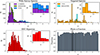 |
Fig. 1. Source breakdown as a function of redshift for objects in our final catalog based on the cuts detailed in Section 3.1. Sources from different methods are shown in different panels: wide field spectroscopic surveys (top left), targeted spectra (top right), and HST Hyperion (bottom left). Rather than including a histogram of photometric redshift counts, we include the photometric redshift fraction (i.e. the fraction of galaxies with only a photometric redshift measured) for reference on the bottom right. The location of Hyperion is included in each panel as a shaded gray region (2.4 < z < 2.7), and insets for this shaded region are included for the spectroscopic and grism redshift panels. Histograms with multiple survey sources are stacked. |
Breakdown of survey sources for all objects in the final catalog.
However, we did make additional cuts for all sources using their IRAC channel 1 (ch1, 3.6 μm) and channel 2 (ch2, 4.5 μm) magnitudes at mIRAC1 < 24.8 or mIRAC2 < 24.8 (roughly 0.03 × M* at z ∼ 2.5, see Weaver et al. 2023). At the redshift of Hyperion (z ∼ 2.5), IRAC ch1 and ch2 correlate strongly with stellar mass by probing rest-frame Y and J bands, respectively, and are largely immune to contributions from dust or young stellar populations. We used both IRAC ch1 and IRAC ch2 (rather than just a single IRAC band) for this cut due to the poor angular resolution of IRAC. The IRCLEAN software (Hsieh et al. 2012) is used to extract photometry from those bands and uses the detection images in other bands as a prior for source extraction. This extraction can result in a non-detection in either IRAC band-pass (particularly for fainter sources), and, thus, to increase the completeness of our final sample we used both IRAC ch1 and ch2. If we were to use only IRAC ch1 for our sample selection, we would lose 10 378 sources or ∼4.7% of our final sample. We chose our IRAC ch1 and ch2 magnitude cuts following the completeness limits for the COSMOS field (see Davidzon et al. 2017; Weaver et al. 2022, 2023) and we chose to make this magnitude cut rather than a stellar mass cut due to the MC process used to obtain our main results (see Section 3.3). This is done to create an overall sample that is stellar mass limited without being reliant on a fitted quantity, as well as to maximize the usefulness of the spectroscopic portion of our sample (i.e., galaxies measured with spectroscopic or grism redshifts in our sample fall off precipitously at IRAC > 24.8). We also found that our main results are invariant to our choice of an IRAC magnitude cut or a LePhare stellar mass cut. We employed the IRAC ch1 and IRAC ch2 values from COSMOS2020 for these cuts and galaxies without measured magnitudes in both IRAC channels by COSMOS2020 are not used.
Additionally, we performed an astrometric cut to limit our sample to the sky region covered by Hyperion (149.6° ≤α ≤ 150.52° and 1.74° ≤δ ≤ 2.73°) utilizing COSMOS2020 astrometry. We also removed all sources designated as stars based on either the spectroscopic catalog or from the COSMOS2020 Classic Catalog LePhare fit (Ilbert et al. 2006; Arnouts & Ilbert 2011). This results in a final sample of 220 356 unique sources. Table 1 gives the source breakdown of our final sample and Figure 1 provides the redshift distribution of our final sample.
In Figure 2, we also provide for reference the stellar mass and the IRAC ch1 magnitude distribution of galaxies in our final sample between 2 < z < 3 (i.e., the redshift range where we examine merger and interaction activity). Values for both the stellar mass and IRAC ch1 magnitude are drawn from COSMOS2020. With our imposed IRAC cuts, the resultant spectroscopic and photometric sample used to assess merger and interaction activity in Hyperion and the surrounding field is roughly 70% complete to a stellar mass limit of log(M*/M⊙) ≳ 9.3 (see also Weaver et al. 2022, 2023).
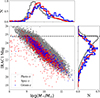 |
Fig. 2. Galaxies in our final sample from 2 < z < 3 plotted in stellar mass and IRAC ch1 magnitude space (lower left) along with individual normalized histograms of stellar mass (top) and IRAC ch1 magnitude (lower right). All values are drawn from COSMOS2020 aside from the redshifts where we employ the best spectroscopic or grism redshift when available. For reference, our imposed IRAC ch1 magnitude cut is plotted as the dotted black line (note: some galaxies in our final sample lie above this line as our IRAC cut is an or cut on both ch1 and ch2). As expected, our spectroscopic and grism redshift sources (spec-z and grism-z, respectively) are primarily at brighter magnitudes and higher stellar masses in comparison to the distribution of photometric redshift only sources. Our final sample has a rough stellar mass limit of log(M*/M⊙)∼9.3 from 2 < z < 3 based on our imposed IRAC cuts. |
Though we do include over 22 000 sources with spectroscopic and/or grism redshifts in our final sample (∼2900 spectroscopic and/or grism sources from 2 < z < 3), the majority of sources in our final sample of 220 356 galaxies are purely photometric sources (∼90%). From Figure 2, we see that the fainter (and low mass) end of our sample from 2 < z < 3 in particular is dominated by photometric sources. This fact in combination with the variety of studies from which we draw spectroscopic redshifts – along with the targeting strategy of HST-Hyperion – suggests the spectroscopic and grism portion of our final sample is subject a complex selection function. Thus, it is important to explore the underlying spectroscopic completeness of our sample as a function of magnitude.
In Figure 3, we plot spectroscopic completeness (or the fraction of sources with a spectroscopic and/or grism redshift, Fspec) as a function of IRAC ch1 magnitude for two distinct populations: the full sample of sources in our final sample from 2 < z < 3 and a sample more specifically targeted to capture the bounds of Hyperion (i.e., the “Hyperion limited” sample). The 2 < z < 3 full sample contains the same sources as shown in Figure 2 and is selected as every source that has their “best” redshift lie within the given redshift range. The Hyperion limited sample contains 3134 galaxies and is selected as all galaxies that have their “best” redshift from 2.4 < z < 2.7 and has an additional astrometric cut of 149.9° ≤α ≤ 150.42° and 2° ≤δ ≤ 2.5° (to match the density contours of Hyperion, see Figure 8). We also include the underlying normalized IRAC ch1 magnitude distributions in Figure 3 for reference.
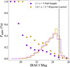 |
Fig. 3. Spectroscopic completeness (or the fraction of sources with a spectroscopic and/or grism redshift, Fspec) as a function of IRAC ch1 magnitude for all sources from 2 < z < 3 in our final sample (purple) and a sub-sample of sources limited to the redshift range of Hyperion with tighter astrometric cuts (gold). Also included for reference are the underlying normalized IRAC ch1 magnitude distributions for each population along with the location of the imposed IRAC ch1 (or ch2) magnitude cut (vertical dashed black line). Spectroscopic completeness for both samples declines sharply as a function of magnitude. However, there is notably higher completeness for galaxies limited more closely to the bounds of Hyperion. |
From Figure 3, we see a sharp decline in spectroscopic completeness as a function of magnitude for both the full sample and the Hyperion limited sample that matches the trends seen in Figure 2. However, we see that the spectroscopic completeness of the Hyperion limited sample is consistently higher than that of the full 2 < z < 3 sample with the Hyperion limited sample seeing ≳10% more completeness until IRAC ch1 ∼23.5 and ∼3 − 5% more completeness until our imposed magnitude cut (i.e., IRAC ch1 < 24.8). Due to the targeting strategies of the included C3VO observations and HST-Hyperion itself, this is expected. Our spectroscopic completeness for both samples is also best where we have lower source counts (IRAC ch1 ≲23) and noticeably lower where the bulk of our sample lies (23 ≲ IRAC ch1 ≲ 24.8). We are sure to account for these varying levels of spectroscopic completeness when making our final close kinematic companion calculations (see Section 3.4.2).
3.2. Environmental measures
3.2.1. Local overdensity
In this work, we differentiate two distinct environments: Hyperion and the coeval field. This definition results from a determination of local overdensity (i.e., log(1 + δgal)) drawn from Voronoi Monte Carlo (VMC) maps made for the Hyperion field (see Tomczak et al. 2017; Lemaux et al. 2017; Hung et al. 2020, 2021; Lemaux et al. 2022; Hung et al. 2025). The Voronoi tessellation technique divides a 2D plane into a number of polygonal regions equal to the number of objects in that plane. A Voronoi cell for each object is then defined as the region closer to it than to any other object in the plane. Objects in the highest-density regions therefore have the smallest Voronoi cells, while objects in lower-density regions have larger cells. The inverse area of the cell sizes can thus be used to measure the local density at the position of the object bounded by the cell.
To obtain the 2D planes for VMC mapping, galaxies are partitioned into thin redshift slices with each slice spanning 7.5 proper  Mpc along the line of sight (approximately 3000–4500 km s−1 or Δz ∼ 0.03 − 0.05 over the redshift range of this study, 2 < z < 3), with a 90% overlap between adjacent slices (see Hung et al. 2020 for a discussion on this choice). Each redshift slice is then projected onto a 2D Voronoi tessellation that is calculated using the positions of the galaxies within it. Local environmental density is defined as the inverse of the area of a Voronoi cell multiplied by the square of the angular diameter distance at the corresponding mean redshift of the slice. The Voronoi maps are then projected onto a 2D grid of pixels sized 75 × 75 proper kpc. The local environmental overdensity at pixel (i,j) is defined as
  where Σi, j is the density at pixel (i, j) and
  is the median density of all the pixels where the map is reliable (i.e., the central 80% of the slice).
A MC process is used to incorporate the redshift uncertainties. The above process of 2D planes partitioned by redshift slices is repeated 100 times, varying the redshifts of the member galaxies in each iteration. Within each iteration, galaxies with a spectroscopic redshift either have that redshift chosen or are cut based on the VUDS-like spectroscopic quality flag (Le Fèvre et al. 2015; Lemaux et al. 2022). Both spectroscopic objects that fail to meet the quality flag cut and objects with no spectroscopic information have a new redshift assigned in each iteration that is sourced from sampling their photometric redshift PDFs in each trial. The voxel values used in final VMC maps are thus the median value of that voxel from these 100 iterations (Hung et al. 2020, 2021; Lemaux et al. 2022). This technique has been employed for a variety of structures across a wide redshift range (0.6 < z < 4.6; Darvish et al. 2015; Shen et al. 2017, 2019; Rumbaugh et al. 2017; Pelliccia et al. 2019; Hung et al. 2020), and is found to be strongly concordant with other density metrics and to trace known structures (Tomczak et al. 2017, 2019; Lemaux et al. 2019; Hung et al. 2025).
3.2.2. Structure definition
Due to the extended nature of high-redshift protoclusters, the possibility exists that the entire field considered in this work may be overdense or underdense in a particular redshift slice, which could bias our overdensity calculations. As such, using the existing VMC maps, we fit a Gaussian to the distribution of overdensity values in each redshift slice, and, based on this fit, calculate the number of standard deviations of a galaxy’s overdensity value above or below the fit mean (σδ; see Forrest et al. 2023, 2024; Shah et al. 2024a for additional information on this calculation). This σδ encodes the 3D statistical significance in overdensity of each particular voxel within our VMC maps and galaxies are assigned overdensity values (and a σδ) based on the nearest Voronoi cell to the galaxy’s coordinates (see Section 3.3.2). Using the σδ values from our VMC maps, we define an overdense structure in a manner analogous to Cucciati et al. (2018), Shen et al. (2021), Shah et al. (2024a), Forrest et al. (2024) by finding all contiguous voxels in our 3D maps with σδ > 2.5 that include extremely overdense peak (σδ > 4, see Sikorski et al. (2025) for the motivation behind these thresholds).
For this study, Hyperion is defined as the most massive overdense structure in our 3D VMC maps from 2 < z < 3 that fits the aforementioned σδ criteria and has a mass of log(M/M⊙)∼15.4 and spans roughly 2.4 < z < 2.7. This structure is similar to the most massive structure first characterized in Cucciati et al. (2018) and the definition of Hyperion used in this work is consistent with Sikorski et al. (2025) There exists other overdense structure from 2.4 < z < 2.7 in our sample and VMC maps, but such structure is associated with separate overdensity peaks and are either unconnected to the structure defined as Hyperion in this work or are connected at low densities (i.e., σδ < 2.5, see Figure 4 and Sikorski et al. 2025 for further discussion). In contrast to our adopted definition of Hyperion and other overdense structure, the coeval field sample used in this work is primarily galaxies at similar redshifts (2 < z < 3) that are not associated with any overdense structure (see Section 3.3.2 and Figure 4).
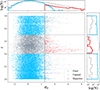 |
Fig. 4. Example of the distribution of galaxies in redshift and overdensity (σδ) space for one MC iteration used in this work (MC #82). Included are only those galaxies in the relevant redshift range for our fraction calculations (i.e., 2 < z < 3). Galaxies associated with Hyperion for this iteration are marked in red and field galaxies for this iteration are marked in blue. Unused galaxies for this iteration are marked in gray (which includes galaxies in the redshift range of Hyperion that are not associated with overdensity and galaxies in the field sample redshift range that are associated with other large structure, see Section 3.3.2). |
3.3. Companion fraction
In order to assess potential merger and interaction activity in Hyperion and the coeval field, we developed a MC methodology to measure the fraction of galaxies with close kinematic companions (fckc). In this methodology, we varied the redshifts of all galaxies in our final sample to find potential companion systems (i.e., galaxies with one or more close kinematic companions) and determined the local environment of such systems. We performed 100 MC iterations based on the following prescription:
-
Vary the redshifts for all sources in our final sample (Section 3.3.1).
-
Determine the environment of all galaxies in the relevant redshift range (Section 3.3.2).
-
Identify galaxies with close kinematic companions (Section 3.3.3).
-
Calculate the fraction of galaxies with close kinematic companions (fckc) for Hyperion and for the coeval field (Section 3.3.4).
Following these steps, we applied a correction factor to obtain our final fckc values (see Section 3.4.2). The choice of this methodology was the result of extensive reliability testing on the feasibility of using photometric redshifts to identify galaxy pairs and galaxies with potential companions. We chose 100 MC iterations to strike a reasonable balance between obtaining a representative sampling of the redshift probability distributions (zPDFs) for our photometric sources and not over-weighing spectroscopic sources. We verified that our 100 MC iterations capture the uncertainty and secondary redshift peaks for a variety of zPDFs (see Appendix A and Figure A.1). The final fckc values reported in this study are the medians of the 100 MC iterations.
3.3.1. Redshift Monte Carlo
We utilized the following procedure to MC the redshifts of our sample for 100 iterations with only galaxies that fall between 2 < z < 3 for that MC iteration being used for further calculations. For each iteration, the redshift variation decision hinged on the type of redshift(s) available and, for sources with a spectroscopic redshift (spec-z) and/or grism redshift (grism-z), the quality flags associated with those redshifts. The 100 MC iterations of the redshifts of our final sample that are detailed in this study are drawn from those presented in Sikorski et al. (2025), and are organized as follows:
-
Galaxies with a spec-z: We either used the available measured spectroscopic redshift or drew from the associated zPDF for that object from COSMOS2020 (v2.0 LePhare fit) for each iteration. To determine whether or not to keep the spec-z or draw from the zPDF, we used the corresponding spectroscopic redshift quality flags. Since we employ the VUDS/DEEP2 quality flag scheme, objects with the highest-quality redshifts (qflag = X3, X4) have their spec-z kept ∼99.3% of the time and sources with other reliable spectroscopic redshifts (qflag = X2, X9) have their spec-z kept in ∼70% of the iterations. Galaxies with low-quality spec-zs (qflag = X0, X1) have their redshifts drawn from the corresponding COSMOS2020 source zPDF each iteration.
-
Galaxies with a grism-z: We used a similar method to that of spec-z sources, where we either drew from a tight Gaussian centered at the grism-z (with a width of 46/14100 × (1 + zgrism), see Forrest et al. 2025), or draw from the source’s COSMOS2020 zPDF for each iteration. For sources with reliable grism redshifts, we sampled from the tight grism-z Gaussian for 93.2% (qfgrism = 5), 80.6% (qfgrism = 4) and 67.4% (qfgrism = 3) of our MC iterations, and draw from the COSMOS2020 zPDF for other iterations. Galaxies with low-quality grism-zs have their redshifts drawn from their COSMOS2020 zPDF each iteration.
-
Galaxies with multiple reliable redshifts: (i.e., a reliable grism-z and a reliable spec-z) We used a hierarchy that prioritizes the most reliable redshifts first. As such, we preferentially used highest-quality spec-zs (99.3% reliable), then the highest-quality grism-zs (93.2% and 80.6% reliable, respectively), then other reliable spec-zs (70% reliable) and finally other reliable grism-zs (67.4% reliable). With this, we employed a similar scheme as already described where, for these sources, we first attempted to take the existing most reliable spec-z or sample from the tight grism-z Gaussian based on the reliability. However, for these sources, if the most reliable spec-z or grism-z was not selected for that iteration, we then utilized the other reliable redshift at a rate that corresponds with its reliability. If neither redshift is chosen, we drew from the corresponding COSMOS2020 zPDF.
-
Galaxies with only a photometric redshift: (photo-z) We drew from the COSMOS2020 zPDF for each iteration.
Once we determined all redshifts for each iteration, we used LePhare to fit the available COSMOS2020 photometry for all galaxies that land in the relevant redshift range (i.e., 2 < z < 3) for that iteration with the redshift fixed to the assigned redshift for that iteration. We used these fits to obtain the stellar masses for each relevant galaxy for each iteration (see Sikorski et al. 2025 for the methodology and substantial discussion).
3.3.2. Environmental determination
Once our redshifts and stellar masses had been determined for each iteration, we also needed to assign the relevant environment for that MC iteration. Thus, for each MC, we identified for each galaxy the σδ corresponding to the nearest voxel based on the galaxy’s astrometric coordinates (COSMOS2020 RA/Dec) and redshift (from that iteration) from the 3D VMC maps that have been created for the COSMOS field (Section 3.2). From these overdensity values, we assigned either “Hyperion”, “field”, or “unused” for each galaxy in redshift range of 2 < z < 3 for that iteration. Galaxies are assigned to Hyperion based on the definition stated in Section 3.2.2 ( galaxies per iteration). All galaxies in the redshift range 2.4 < z < 2.7 that are not assigned to Hyperion are designated “unused” to mitigate the effects of galaxies potentially infalling into the Hyperion structure (see Staab et al. 2024) or galaxies that are associated with other nearby overdense peaks (Cucciati et al. 2018). Field galaxies are thus all sources outside the redshift range of Hyperion (2 < z < 2.4 or 2.7 < z < 3) that are not a part of any significantly massive overdense structure (i.e., do not belong to any σδ > 2.5 voxel that is contiguously connected to a σδ > 4 voxel with an overall structure mass of log(M*/M⊙) > 13). This excludes from our field sample galaxies that belong to other known structures in the COSMOS field at relevant redshifts and astrometric coordinates (Diener et al. 2013; Cucciati et al. 2014; Lemaux et al. 2014; Yuan et al. 2014; Casey et al. 2015; Chiang et al. 2015; Franck & McGaugh 2016; Lee et al. 2016; Wang et al. 2016; Cucciati et al. 2018; Lemaux et al. 2018; Darvish et al. 2020; Koyama et al. 2021; Polletta et al. 2021; Ata et al. 2022; Newman et al. 2022; Hung et al. 2025). This removal of galaxies in known structures from the field sample is done to help isolate the effect of the overdense Hyperion structure in comparison to field galaxies that are not associated with overdense environments. Unused sources for each MC iteration also include galaxies outside the redshift range considered in this work (i.e., 2 < z < 3). In total, unused sources are galaxies outside the relevant z-range, galaxies within the z-range of Hyperion that are not associated with the massive overdense peak, or galaxies that are associated with other large structures in redshift ranges of our field sample. An example of the a full MC of galaxies from this work can be seen in Figure 4.
3.3.3. Companion identification
For each MC iteration, we identified all galaxies with potential companions based on their physical location for that iteration. For this, we followed the typical procedure within the literature and select potential companion galaxies based on on two primary factors: projected spatial separation and velocity difference of the member galaxies (see Lambas et al. 2003, 2012; Robotham et al. 2014; Ferreras et al. 2017; Nottale & Chamaraux 2018). Similar to Shah et al. (2020, 2022), we define companion galaxies as galaxies that are within dproj < 150 kpc and ΔvLoS < 1000 km s−1 of another galaxy. While other studies only consider maximum projected separations of companion galaxies to be in the range of 80–100 kpc (Patton et al. 2011; Scudder et al. 2012; Ellison et al. 2013b), we opt for a larger value of 150 kpc as there are studies that show that interacting galaxies begin to impact one another at such distances (Patton et al. 2013; Shah et al. 2020, 2022), and, as we are interested in future merger and interaction activity in this work, galaxies in our redshift range of 2 < z < 3 at distances of ∼150 kpc have ample time to merge by z ∼ 0 (see Section 4.2). Additionally, we found that our results are invariant with respect to the choice of a lower projected separation criteria, and that a ≳2σ difference in measured fckc between the field and Hyperion persists at smaller rproj (see Section 4, as well as Section 4.2 and Table 4).
Projected separations for companion galaxies were calculated by multiplying the angular separation between the two galaxies by the angular diameter distance of the average redshift of the two galaxies (dproj ≡ θsep * DA). Line-of-sight (LoS) velocities are calculated based on the redshift of each galaxy for that MC iteration. At the redshift range of Hyperion, a ΔvLoS < 1000 km s−1 corresponds to a Δz ≲ 0.01 between two galaxies and a dproj < 150 kpc corresponds to Θsep ≲ 18″. An example of a galaxy with an identified companion based on our selection criteria can be seen in Figure 5. We chose to plot both a 2D and 3D representation of the same galaxy to highlight the importance of our LoS velocity criteria, as that cut is the most crucial in identifying projected companions versus potential true companions – particularly in sky regions of higher galaxy number density.
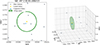 |
Fig. 5. On-sky 2D view and 3D reconstruction of a potential galaxy companion for COSMOS2020 (C20) object #1006523 found during our MC process (MC iteration #87). The central galaxy (C20#1006523) is marked in gold with our 150 kpc search radius centered on that galaxy shown in green. The companion galaxy that meets both the projected separation and LoS velocity difference criteria is denoted in blue. Other nearby galaxies are shown in gray. While multiple galaxies fall within the projected separation criteria for this galaxy, the 3D LoS velocity difference cut helps isolate the single companion from other projected companions. |
We did not make any cuts on the galaxy mass ratio during the companion identification process, but we did cut our final sample of companion systems used for all calculations to only consider major interactions or mergers. To be consistent with the literature, we adopted the definition of mass ratios less than 4 (4:1) to be major interactions and/or mergers and all others to be minor interactions and/or mergers (e.g., the ratio of the mass of the most massive galaxy to the mass of the least massive galaxy, see Ellison et al. 2013a and Mantha et al. 2018). The stellar masses for calculating these mass ratios are the result of the LePhare SED fitting described in Sikorski et al. (2025) and are based on the redshifts obtained in the MC process.
3.3.4. Fraction calculation
For each MC iteration, we calculated a fraction of close kinematic companions (fckc) for both Hyperion and the coeval field considering only galaxies that have companions that would result in a major iteration and/or merger (≤4:1 in mass ratio). This calculation is simply done by taking the unique number of galaxies with companions or that are companions (to mitigate galaxies with multiple potential companions; ∼14.0 ± 8.9% of Hyperion companion galaxies over our 100 MC iterations and ∼3.6 ± 0.8% of field companion galaxies) divided by the total number of galaxies in Hyperion or the field for that MC iteration (fckc = Ncompanions/Ngals). This gives us our uncorrected companion fractions for each MC iteration. Typically, Ncompanions ∼ 43 galaxies for Hyperion and ∼1141 galaxies for field. We then take the median fckc over these 100 MC iterations as the final uncorrected companion fraction: 14 ± 1.8% for Hyperion and 5 ± 0.2% for the field (with the associated error on this measurement being the 1σ spread of the 100 MC iterations, see Section 3.4.2 for full error budget).
3.4. Simulated lightcone
In order to validate and make any potential corrections to our companion methodology, we applied our MC methodology to simulated galaxy observations where the “true” fckc is known. For this, we employed the GAlaxy Evolution and Assembly (GAEA; Hirschmann et al. 2016; De Lucia et al. 2024) semi-analytic model (SAM) to generate simulated galaxy catalogs. We used the GAEA model version described in Xie et al. (2017)1, and applied it to the dark matter merger trees of the Millennium Simulation (Springel et al. 2005). We followed the procedure of Zoldan et al. (2017) to generate a lightcone from the output of the GAEA SAM. The simulated lightcone used in this work is identical to the one used in Hung et al. (2025).
More specifically, we used the 1 × 1 deg2 field denoted “Mock1” from Hung et al. (2025) cut at IRAC/ch1 < 24.8. We chose to use this portion of the simulated lightcone as there are multiple versions of this region created with at different levels of spectroscopic redshift fraction (SzF). To create these different lightcone versions at varying SzF, Hung et al. (2025) broke down that region of the lightcone into bins of magnitude and redshift, and, using statistics that compared the spectroscopic and photometric redshifts within the COSMOS field (see Lemaux et al. 2022), generated “observed” spectroscopic catalogs using different SzF selection functions as a function of the magnitude and redshift from the COSMOS field. Spectroscopic redshifts were assigned randomly to galaxies in each given magnitude and redshift bin (the former of which were chosen to roughly contain an equal number of objects in each bin) and spectroscopic quality flags were assigned to mimic the distribution of quality flags in the real data. The base SzF level for this selection function (SzF 1.0) was modeled at the underlying level of the COSMOS field spectroscopic completeness at the time of the mock catalog creation (∼7%, Hung et al. 2025). The other SzF fractions can be found in Table 2 representing the five different Mock1 simulated lightcone catalog versions.
Mock lightcone and validation statistics.
All objects within each version of the Mock1 region were also assigned a photometric redshift regardless of whether or not they were assigned a spectroscopic redshift using the following formula: zphot = zobs + B(1 + zobs)+Nσpz(1 + zobs), where B is the spectroscopic to photometric redshift bias in the galaxies magnitude and redshift bin, N is a value sampled from a normalized Gaussian distribution for each object, and σpz corresponds to the σNMAD of the photometric redshift scatter within that bin. Photometric redshift uncertainties (at ±1σ) for each simulated galaxy were drawn from the PDF of the fractional photometric redshift error (i.e., (zphot, 1σ, upper − zphot)/(1 + zphot) and (zphot − zphot, 1σ, lower)/(1 + zphot)) that was calculated through the statistics of objects in each magnitude bin in the real COSMOS data (Lemaux et al. 2022). Thus, at the end of this process each simulated galaxy had a photometric redshift with an associated ±1σ uncertainty. The photometric redshifts generated via this parametrization can be seen in Figure 6 for relevant galaxies from the Mock1 region of the simulated lightcone (i.e., from 2 < zobs < 3).
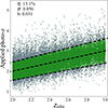 |
Fig. 6. Applied photometric redshifts (photo-zs) versus true simulation redshifts (zobs) for all galaxies in the Mock1 region of the simulated lightcone between 2 < zobs < 3. Galaxies that meet |Δz|< 0.15(1 + zobs) are marked in green (Hildebrandt et al. 2012). The statistics for these galaxies are listed in the upper right hand corner (outlier fraction, scatter, and bias, respectively). Photo-zs are applied to all galaxies in our simulated lightcone based on the observed photo-z statistics in COSMOS2020 as a function of magnitude and redshift. The scatter in photo-zs creates difficulty in recovering companion systems (see Section 3.4.1). |
3.4.1. Lightcone validation
We applied our MC companion methodology to each version of the Mock1 catalog (i.e., at each different SzF) using an identical method to that detailed in Section 3.3 – aside from the determination of environment – in order to estimate how accurately our methodology can recover true galaxy companions based on our observational definition at different levels of spectroscopic completeness. For each Mock1 SzF catalog, we performed 100 MC iterations looking for galaxy companions in the redshift range 2 < z < 3 (i.e., the same redshift range we used for our real observed data). While we tracked companions of all mass ratios, we again considered only companion systems that would potentially result in a major merger or interaction (maximum mass ratio of 4:1) to be consistent with the operational definition adopted for our observed data on what types of systems are included in our fckc and other calculations.
To assess our recovery of true companion galaxies, we used the true redshifts given from the simulation, zobs, a value that incorporates peculiar velocities, and find all galaxies with major companions based on our criteria given in Section 3.3.3. From this, we obtained the true fckc of 24.3% for the simulated galaxies in the lightcone over 2 < zobs < 3 (a value consistent with the literature, see Figure 9). We then calculated the median purity and median completeness of the companion galaxies identified in our 100 MC iterations at each SzF based on the true companion galaxies in the lightcone. As expected, we find that both the median purity and median completeness of companion galaxies identified with our MC methodology increase with SzF as, at lower levels of spectroscopic completeness, larger numbers of galaxies are assigned “observed” photometric redshifts that obscure their true location (which are randomly scattered from their true redshift; see Figure 6) which in turn greatly reduces the likelihood they are identified as companions in our methodology or causes them to be identified in false companion systems. The median purity and median completeness of the companion galaxies identified in our application of the MC methodology at each SzF can be found in Table 2 and in Figure 7 (upper panel).
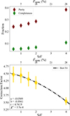 |
Fig. 7. Top: Median purity and median completeness of companion galaxies identified via the application of our MC methodology on the Mock1 lightcone at different levels of SzF. Bottom: Correction factor |
3.4.2. Correction factor
With our MC companion methodology, we see an increase in both the purity and completeness of identified companion galaxies as a function of SzF. This is expected as in our methodology quality spec-zs (which are measured at zobs for the simulated lightcone data) are often kept as the measured redshift value, which in turn results in more frequent recovery with our companion criteria (even a variation of Δz = 0.05 results in no companion) and thus higher completeness and increased purity. However, the purity and completeness achieved with our MC methodology does not approach unity – even at 28% spectroscopic completeness – resulting in the derivation of a correction factor to adjust for the identification of false positives and the lack of true recovery of companion galaxies. We constructed this correction factor to be equivalent to the median purity divided by the median completeness of identified companion galaxies at a given SzF. These correction factors can be found in Table 2 and Figure 7 (bottom panel). We used these calculated correction factors to inform the choice of our final correction factors for the Hyperion and the field.
However, SzF is not constant as a function of astrometric coordinates in our final sample, as the C3VO and HST-Hyperion observations are specifically targeted at the overdense peaks in the Hyperion structure which increases the SzF non-uniformly in RA/Dec space. To explore this effect, we plot SzF as a function of RA/Dec in Figure 8 in 20 × 20 even bins of RA and Dec (approximately ∼2.8′×3.0′) for all galaxies in our final sample with a photometric redshift in the range 2 < z < 3. Plotted for reference are the σδ > 2.5 and σδ > 4 contours of the overdense structure that comprises Hyperion in this work compressed into two-dimensions (i.e., the regions used for the Hyperion fckc).
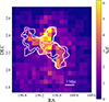 |
Fig. 8. SzF for sources with a photo-z with 2 < z < 3 in our final sample in 20 × 20 bins of even RA and Dec (each bin is approximately ∼2.8′×3.0′). Over-plotted are the 2.5σδ and 4σδ contours of the massive structure defined as Hyperion in this work. As expected from the underlying spec-z surveys used in this study, we see increased SzF in the regions covered by the Hyperion overdensity finding a median SzF of ∼1.78 for Hyperion and a median SzF of ∼0.67 for the field. These median SzFs are used to determine the final correction factors applied to our uncorrected fckc values. |
Using the 20 × 20 RA/Dec grid seen in Figure 8, we calculated a median SzF for pixels inside the Hyperion contours (SzF-Hyp) and a median SzF for pixels outside of the SzF contours (SzF-Field). From this, we obtain an SzF-Hyp ∼1.78 (Fspec ∼ 12.4%) and an SzF-Field ∼0.67 (Fspec ∼ 4.7%). We translate these SzF values to the proper correction factors needed to correct the “raw” Hyperion fckc and field fckc by interpolating between the calculated correction factors via the second-order polynomial fit seen in Figure 7). The correction factor estimates based on this fit and the median SzF of Hyperion and the field are ∼4.25 and ∼4.46, respectively, and are applied to our uncorrected fckc values to obtain our final fckc measurements. Due to the large difference already present in our uncorrected companion fractions (see Section 3.3), our results are immutable to our choice of correction factor over the range of SzF considered in this work.
We carefully account for the uncertainties in our median SzF estimation for Hyperion and the field and its impact on the chosen correction factor, along with the variation in correction factor from applying our MC methodology to the lightcone data (i.e, the variation in the purity and completeness of our identified companion galaxies), into the final error budget of our fckc measurements. To incorporate these uncertainties, we combined all three sources of error in quadrature: (1) the scatter in correction factor from the lightcone at a given SzF, (2) the variation in correction factor based on the σNMAD of the SzF in Hyperion and the field, and (3) the median scatter in uncorrected fckc for Hyperion and the field. The resulting error is then applied to our corrected fckc values to determine the final uncertainties reported in Section 4.
4. Results
By applying the correction factors derived in Section 3.4.2 to our uncorrected companion fractions from Section 3.3, we obtain a final fckc for Hyperion and a final fckc for the field. We find a ≳2.5× enhancement in fckc for galaxies in the overdense structure of Hyperion with over half of all Hyperion galaxies having a nearby companion, as we measure a corrected fckc =  % for Hyperion and an fckc =
  % for the field (a ≳3σ difference). Though an overdense region similar to Hyperion naturally suggests higher fckc – due to many galaxies existing in relatively close proximity – this measurement properly validates that intuition. Additionally, protoclusters at the epoch of Hyperion are still diffuse systems that span many cMpc and sometimes wide redshift ranges (Δz ∼ 0.5 in the case of Hyperion), so satisfying our stringent companion criteria is not easy; particularly in the LoS direction where galaxies are required to be tightly correlated in redshift space (Δz ≲ 0.01).
Though there are relatively few studies in the literature that examine quantities similar to fckc at a relevant redshift range to this work (2 < z < 3), we note that the field fckc derived in this study is in good agreement with other predictions for major merger and interaction fractions, demonstrating the validity of our applied technique (see Figure 9). The dearth of other studies is often attributed to the lack of spectroscopic coverage to confirm galaxies with companions or to the lack of completeness in photometry which makes probabilistic methodologies more difficult. However, we do wish to acknowledge that the methodologies for investigating companions, interactions, and merger activity (i.e., close pair and morphological studies) in the literature are varied, and there is no consensus on the best approach, as data quality and availability varies greatly – particularly for methods that attempt to include sources with photo-zs. We do our best to compare to values in the literature with as similar companion selection criteria to those employed for our fckc methodology whenever possible.
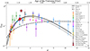 |
Fig. 9. Evolution of fckc and fckc-like measurements as a function of redshift. The values measured in this work are plotted in red with black borders with the star denoting our structure measurement and the circle denoting our field measurement. Other studies that examine merger and interaction rates in relation to overdensity or structure at relevant epochs have their results plotted similarly (i.e., structure or overdensity fraction as a star and field fraction as a circle, Hine et al. 2016; Monson et al. 2021; Liu et al. 2023; Shibuya et al. 2025) Various values from the literature that measure relevant major merger and pair fractions are also plotted for reference (Bundy et al. 2009; Conselice et al. 2009; de Ravel et al. 2009; Xu et al. 2012; López-Sanjuan et al. 2013; Tasca et al. 2014; López-Sanjuan et al. 2015; Ventou et al. 2017; Duncan et al. 2019; Romano et al. 2021; Duan et al. 2025), along with simulation predictions from Qu et al. (2017) and empirical fits from Romano et al. (2021) and Duan et al. (2025). Overall, we find that fckc evolves sharply at low redshift before peaking at z ∼ 4 with the measured fckc for Hyperion, though at lower redshift (z ∼ 2.5), existing above the peak value. Though some scatter exists, the existing measured merger and interaction rates for structures and overdensities are higher than the corresponding field rates at similar redshifts. |
We also wish to highlight the only three other studies in the literature that explore merger and interaction activity in high-z (z > 2) protoclusters from Hine et al. (2016), Monson et al. (2021), and Liu et al. (2023). The most recent work, Liu et al. (2023), finds a similar enhancement in merger and interaction activity in both of their structures (BOSS1244 and BOSS1542) in comparison to their coeval field sample, but their search is limited to only high-mass (log(M*/M⊙)≥10.3) Hα emission-line (HAE) galaxies. Hine et al. (2016) and Monson et al. (2021) both employ observations from the Hubble Space Telescope (HST) to study the SSA22 protocluster at z = 3.1. However, these two studies obtain marginally discrepant results when assessing mergers within SSA22 with Hine et al. (2016) finding an ∼1.5σ enhancement in merger activity in the protocluster relative to the field and Monson et al. (2021) finding statistically equivalent rates of mergers in the field and protocluster. As discussed in Monson et al. (2021), the potential difference in the two results is likely due to small number statistics in combination with the different rest-frame wavelength ranges probed by each study for their morphological merger classification (rest-frame UV from HST/ACS F814W imaging for Hine et al. (2016) and rest-frame optical from HST/WFC3 F160W for Monson et al. 2021). Overall, these three studies offer the most relevant comparisons to this work and are statically in agreement with our results, though with large uncertainties in each case. Our study includes an order of magnitude more galaxies both in terms of overall sample and potential identified galaxies with companions resulting in much tighter uncertainty intervals. The fractions derived in Hine et al. (2016), Monson et al. (2021), and Liu et al. (2023) are included along with their field fractions in Table 3.
Relevant merger rates and pair fractions in the literature.
Also included in Table 3 is the results of Shibuya et al. (2025). This study measures the major merger fraction for galaxies in regions of different galaxy overdensity ( ) in the ∼300 deg2 area of the combined HSC Strategic Survey Program (Aihara et al. 2018a,b, 2019, 2022) and CFHT Large Area U-band Survey (Sawicki et al. 2019) and thus is of interesting comparison for this work. Shibuya et al. (2025) find a roughly linear increase in the fraction of major mergers as a function of overdensity from z ∼ 2 − 5, but the relative increase in merger fraction with increased density is marginal. This overall increase in the merger fraction with increased density aligns well will the results of this study, though the fractional increase in merger and interaction activity indicated by our fckc measurements is much greater. However, a direct comparison in these terms between our work and Shibuya et al. (2025) is difficult as they report their measured merger fractions at different average levels of galaxy density (
 ) rather than at a structure versus field level (a δ ≳ 0.62 roughly corresponds with the threshold we use to discern between structure and field populations based on our VMC mapping technique and definition of structure, see Section 3.2.2). Additionally, Shibuya et al. (2025) employ only photo-zs in their calculations which can create issues in separating out what galaxies belong to a field versus structure population (Hung et al. 2020, 2025).
To summarize our findings in comparison to both other environmental studies and to general merger and interaction studies in the field, we plot our measured fckc values along with various major pair and major merger rates from the literature as a function of redshift in Figure 9. For this figure, we use the studies (and selection criteria) chosen in Romano et al. (2021) along with additional relevant selections from the literature to expand the redshift range and to display the other previously discussed studies that consider environment when calculating their pair and/or merger fractions. For included studies that do consider environmental implications, the assumptions and methods for their field measurements and structure measurements are the same, but the assumptions and applied methodology across studies – regardless of environmental consideration – can vary greatly. Thus, it can be difficult to make specific comparisons between studies though some general trends can be found. From newly obtained measurements of the early Universe (z > 6; Duan et al. 2025), we see a slight evolution of the fraction of merging and interacting galaxies that eventually peaks at z ∼ 4 with a strong drop off in the local Universe after z ∼ 2. This evolution roughly maps the currently known cosmic star-formation history (Madau & Dickinson 2014; Harikane et al. 2023, 2024, 2025) and AGN history (Aird et al. 2015; Kulkarni et al. 2019) of the Universe, though offset to slightly higher redshifts. However, the corrected fckc value measured for Hyperion at z ∼ 2.5 is above the peak of merger and interaction activity at z ∼ 4, and significantly above similar values for the coeval field. In combination with the sparse other literature measurements that are also mostly enhanced compared to the field, this result suggests that merger and interaction activity is more prevalent in dense environments at higher redshifts (z > 2) when structure is still forming and developing.
Given the wide breadth of companion selection criteria currently used in the literature, and to help facilitate future comparison, we also will report corrected fckc values for Hyperion and the field cut at rproj < 50 kpc and at rproj < 100 kpc. To calculate these fckc values, we take our same MC iterations for both the observed data and lightcone data, but cut all identified companion systems at larger projected separation criteria. We then perform the same SzF fitting as seen in Figure 7 for the recovered lightcone companion galaxies at this rproj limit and interpolate to the median SzFs of Hyperion and the field given in Section 3.4.2. We apply these updated correction factors to the “raw” companion fractions from the observed data based on the smaller rproj cuts with the same total error considerations to obtain our final corrected fckc values and errors at reduced projected separations. We find that our result of enhanced merger and interaction activity in Hyperion is not sensitive to the choice of projected separation criteria, and calculate a fckc
 % for Hyperion and a fckc
 % for the field at rproj < 100 kpc. Similarly, we recover a fckc
 % for Hyperion and a fckc
 for the field at rproj < 50 kpc. While our field fckc values begin to deviate from other measurements in the literature at smaller separations, there are additional assumptions we are unable to control for between all studies (namely sample selection and any correction or weighting scheme), and our trend of a significant (≳2σ) increase in merger activity in Hyperion relative to the coeval field still holds.
We also include Figure 10 to compare the distributions of projected separation (dproj), LoS velocity (ΔvLoS), and stellar mass ratio between companion systems found in Hyperion and the coeval field. The plotted distributions are normalized for easier comparison and contain all companion systems found over each of our 100 MC iterations (i.e., companion systems identified in multiple iterations are included multiple times). Over our 100 MC iterations, we see a few trends emerging between companion systems found in Hyperion versus companion systems found in the field. Whereas the occurrence of close kinematic companions for the field monotonically increases with dproj, we find increased numbers of companion systems at dproj ∼ 40 kpc and dproj ∼ 125 kpc for Hyperion. We also find that the underlying distribution of ΔvLoS for companion systems in the field is roughly uniform while companion systems in Hyperion are more tightly correlated in redshift space with many companion systems existing at ΔvLoS < 250 km/s. Lastly, companion systems in the field see a monotonic decrease with stellar mass ratio in contrast to the buildup of companion systems at M* ratio ∼1 for Hyperion. However, since Hyperion sees an increase in spectroscopic completeness in comparison to our field sample, some of the observed trends in the companion system parameters for Hyperion are likely the result of more consistent redshifts being used in our MC process which results the preservation of the same companion systems across MC iterations. Further implications of the differences in these underlying distributions for companion systems in Hyperion and the field are discussed in the following sections (i.e., Section 4.1 and Section 4.2).
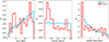 |
Fig. 10. Normalized distributions of projected separation (dproj; left), LoS velocity (ΔvLoS; center), and stellar mass ratio (right) between companion systems found in Hyperion (red) and the coeval field (blue). The plotted distributions contain all companion systems found over each of the 100 MC iterations used to identify close kinematic companions, so companion systems identified in multiple iterations are plotted multiple times. As opposed to the uniform and monotonic distributions seen for companion systems in the field, companion systems in Hyperion exhibit more complex distributions of dproj, ΔvLoS, and stellar mass ratio. |
4.1. Tidal strength
In order to quantify the impact of any potential interaction activity for companion galaxies found in this study, we utilize the tidal strength Q that companion galaxies produces on a central (more massive) galaxy (Dahari 1984; Verley et al. 2007a,b; Sabater et al. 2013; Argudo-Fernández et al. 2013, 2014). This tidal strength parameter attempts to quantify the relationship between the tidal forces exerted on the galaxy,
 (1)
(1)
and the internal binding force of galaxy,
 (2)
(2)
making the tidal strength, Q, equivalent to the ratio of these forces,
 (3)
(3)
where Mi and MP are the stellar masses of the companion and primary galaxy, respectively. DP is the apparent diameter of the primary galaxy, and RiP is the projected physical distance between companion and primary galaxy (Ri, p ≡ rproj). The total tidal strength is thus the summed tidal strength exerted by all companions and is defined as
 (4)
(4)
This logarithm of the sum of the tidal strength created by all nearby companions is thus a dimensionless estimate of the gravitational interaction strength (Verley et al. 2007a), and generally varies between −5 and +2 depending on the mass ratio and projected distance to companion galaxies. Based on this definition of Q, the tidal forces exerted by the companion galaxy on the primary galaxy is equivalent to the binding forces only when Q ≥ 0. However, based on the results of numerical simulations (Athanassoula 1984; Byrd & Howard 1992), as well as observational results (Varela et al. 2004), perturbations may be induced by external tidal forces from companion galaxies when those tidal forces amount to at least 1% of the internal binding force (i.e., Q ≥ −2).
For each of our 100 MC iterations, we calculated the median tidal strength ( ) for all galaxies with companions in the field and in Hyperion. If there are multiple companions in nearby proximity, we find the tidal strength on the most massive galaxy in every system of companions. For this calculation, we used the masses derived in Section 3.3.1 and the projected distances calculated in Section 3.3.3. For the apparent diameter of the primary galaxy (DP), we use 2 × r80 with r80 being estimated from Equation (2) of Mowla et al. (2019) using their best fit parameters from 2 < z < 2.5 or 2.5 < z < 3. From the individual
  values from each of the 100 MC iterations, we calculated the median
  over all 100 MC iterations (
 ) for both companion systems in Hyperion and companion systems in the field. We find a
  for Hyperion companion systems and a
  for the field companion systems. Thus, the tidal strength exerted by companion galaxies in Hyperion (via
  ) is on average enhanced by ∼0.4 dex (∼2.5×) in comparison to the tidal strength exerted by companion galaxies in the field. This comports with the higher average fraction of galaxies with multiple companions in Hyperion (∼14.0 ± 8.9% relative to ∼3.6 ± 0.8% for the field) along with the higher average fraction of companion galaxies within closer proximity in Hyperion (dproj < 50 kpc; ∼28.0 ± 6.5% for Hyperion and ∼17.6 ± 1.4% for the field; also see Figure 10), as those are the key factors in determining the exerted tidal strength.
In Figure 11, we plot the dependence of the tidal strength (Q) on the projected physical distance between companion and primary galaxy (Ri, p) for a variety of mass ratios considered in this work along with the  values for Hyperion and the field. Though we consider a wide range of projected physical distances when selecting companions, the exerted tidal forces only outweigh the binding forces when Ri, p ≲ 10 kpc. The
  exerted by companion galaxies in Hyperion over our 100 MC iterations is indeed stronger than the
  exerted by companion galaxies in our field sample over 100 MC iterations, but neither value indicates a population of companion systems dominated by those which are necessarily inducing extreme tidal forces (i.e., Q ≥ 0). Rather both the companion systems within Hyperion and within the field are primarily well below this threshold and typically have larger physical separations (
 kpc). Therefore, we calculated the median fraction of companion systems where Q ≥ −2 (i.e., the minimum threshold to induce perturbations) over our 100 MC iterations for Hyperion and for the field (
 ) finding a
  % for Hyperion and a
  % for the field. This suggests that the companions within Hyperion are on average inducing more instabilities than their counterpart companion galaxies in the field.
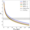 |
Fig. 11. Dependence of the Q (tidal strength) on Ri, p (the projected physical distance between companion and primary galaxy) for range of companion mass ratios considered in this work. The Q value contours are estimated using the typical size of a star-forming galaxy at z ∼ 2.5 from Ribeiro et al. (2016). Also included for reference are the |


4.2. Potential merger timescales
As we select galaxies with close kinematic companions in our sample to estimate future merger activity – rather than selecting galaxies currently undergoing mergers through morphology – it is important that we attempt to quantify the potential timescales associated with any future mergers. We primarily focus on major mergers within this work, so this timescale gives an indication of the timescales by which these galaxies will grow significantly in stellar mass (either through induced star formation or upon coalescence). However, since we consider a wide range of projected physical distances and LoS velocity differences for our companion criteria, calculating a single merger timescale for all close kinematic companions found in our sample is too simplistic and does not accurately capture the full distribution of potential merger timescales.
To calculate the associated merger timescales of the close kinematic companions identified within the 100 MC iterations of our sample, we used the formalism described in Kitzbichler & White (2008)
 (5)
(5)
For this equation, Kitzbichler & White (2008) (hereafter KW+08) performed a two-dimensional linear regression fit on simulated galaxy pair catalogs from the Millennium Simulation to obtain ⟨Tmerge⟩ as a function of stellar mass threshold (for both galaxies) and redshift for major merger systems and provide six discrete sets of coefficients that vary based on the applied companion identification criteria (i.e., projected separation, rproj, and LoS velocity difference, ΔvLoS). The selected rproj and ΔvLoS values that create these fitting coefficients are intended to capture a representative range of projected physical distances used in companion studies (i.e., maximal values of 30, 50 or 100 kpc h−1) and for application to both spectroscopic redshift samples (ΔvLoS < 300 km s−1) and photometric redshift samples (ΔvLoS < 3000 km s−1). The employed companion criteria, and thus the fitting coefficients, have a notable impact on the measured values of ⟨Tmerge⟩ (see Figure 12).
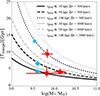 |
Fig. 12. ⟨Tmerge⟩ as a function of stellar mass. Contours represent the six different companion selection criteria and corresponding fitting coefficients from Kitzbichler & White (2008). These contours are all plotted at the median redshift of all pairs over all MC iterations (z ∼ 2.48). We also include the calculated ⟨Tmerge⟩ values for Hyperion (red) and the field (blue) at each of projected separation criteria employed (i.e., rproj ≤ 30 kpc (squares), 30 < rproj ≤ 50 kpc (diamonds), and 50 < rproj ≤ 150 kpc (crosses)). The ⟨Tmerge⟩ values calculated for Hyperion are shorter in each bin due to the larger stellar masses of galaxies in Hyperion companion systems. |
Though we used different criteria in selecting our sample of companion galaxies across our 100 MC iterations, we attempt to mimic the selection criteria of KW+08 when calculating ⟨Tmerge⟩ values. To do this, we split our identified companion systems into three bins of projected physical distance (rproj < 30 [kpc], 30 < rproj < 50 [kpc], and 50 < rproj < 150 [kpc]) for the companion systems in Hyperion and companion systems in the field for each of our 100 MC iterations (i.e., six samples per MC iteration). We then compute the median LoS velocity difference within each of those six bins over all 100 MC iterations, and find that the typical ΔvLoS for each sample is ≲500 km s−1 (see Table 4 and Figure 10). Based on these values, we decide to utilize the coefficients based on ΔvLoS < 300 km s−1 for calculating ⟨Tmerge⟩. We believe this choice is justified as, though we employ a sample of both spectroscopic and photometric redshifts, our MC methodology mitigates the effect of large photometric redshift errors and enforces a stringent ΔvLoS criteria that is in line with studies that only employ spectroscopic redshifts across similar redshift ranges (e.g., Shah et al. 2020, 2022). We also calculate the median galaxy stellar mass ( ) and the median redshift (
 ) for all companion systems in our six bins across the 100 MC iterations.
Using the appropriate rproj and ΔvLoS coefficients per the mimicked companion selection criteria (i.e., rproj ≤ 30 kpc & ΔvLoS < 300 km s−1, rproj ≤ 50 kpc & ΔvLoS < 300 km s−1, rproj ≤ 150 kpc & ΔvLoS < 300 km s−1) along with our measured  and
and  values, we calculated the ⟨Tmerge⟩ for each of our six bins (values reported in Table 4, also see Figure 12). As expected, we find that ⟨Tmerge⟩ decreases with decreasing rproj for both companion systems in Hyperion and companion systems in the field with the companion systems of projected separations of less than 30 kpc having the shortest merger timescales. However, for every bin of projected separation, the average merger timescale for companion systems in Hyperion is shorter than the average merger timescale for the corresponding companion systems in the field. Though a slight offset exists in
  between the Hyperion and field companion systems, we control for variations in the projected separation through our binning and thus the measured difference in ⟨Tmerge⟩ between our Hyperion and field companion systems is primarily due to the varying
  between companion systems in Hyperion and the field. The increased stellar masses for systems in Hyperion results in faster merger timescales in comparison to the field and comports with the increased stellar masses seen in Hyperion (Sikorski et al. 2025).
We also calculated the median fraction of companion systems within each bin ( number of systems at that projected separation divided by the number of total companion systems). This calculation gives us insight into what fraction of companion systems in Hyperion and in the field should be associated with a given merger timescale. Through this calculation, we find similar fractions of companion systems within our smallest projected separation bin (∼8% within rproj ≤ 30 kpc), but diverging fractions of companion systems in our other projected separation bins. Most notably, in the intermediate projected separation bin (30 < rproj < 50 kpc), Hyperion companion systems that meet this criteria account for ∼20% of companion systems across all 100 MC iterations whereas field companion systems in this bin only account for ∼10% of companion systems. Due to the higher density of Hyperion, this is not necessarily surprising, but, since we do not observe a corresponding increase in companions systems within the smallest projected separation bin, this increase in companion systems at intermediate separations is likely physical and supports the increased merger and interaction activity measured by the fckc values found in this work. In fact, the lack of a corresponding increase in companions systems within the smallest projected separation bin in Hyperion could be the result of the closest companion systems having already merged, as this process could accelerated compared to the similar field systems due to increased stellar mass. This is further corroborated by the median σδ (
 ) associated with our projected separation binned companion systems (see Table 4;
  for all Hyperion galaxies both with and without companions over the 100 MC iterations and
  for all field galaxies). Whereas we find a relatively flat trend in
  for companion systems in the field, there is a notable jump in
  for companion systems with intermediate projected separations in Hyperion that suggests the most dense regions are sites of increased merger and interaction activity.
In Figure 12, we plot the evolution of ⟨Tmerge⟩ as a function of stellar mass. To further demonstrate the important contribution of the selected fitting coefficients, we include contours at all six permutations of companion separation criteria from KW+08. As is evident from these contours, the rproj and ΔvLoS criteria that provide these coefficients have a significant impact on the resulting measurement of ⟨Tmerge⟩ – especially at lower companion stellar masses. We also plot the location of our calculated ⟨Tmerge⟩ values for Hyperion (red) and for the field (blue). As discussed above, the increased stellar masses seen in the galaxies that comprise the Hyperion companion systems is primarily responsible for their faster merger timescales in comparison to the field. This increase in timescale is most notable for the largest projected separation bin, but the intermediate projected separation bin sees the largest difference in median stellar mass.
The range of ⟨Tmerge⟩ values calculated in this work follows the wide range of allowed projected separations (i.e., rproj < 150 kpc) used to identify companion systems within our MC methodology. Though the merger timescales associated with companion systems at the widest projected separations are ∼10 Gyr, the age of the Universe at the redshift range of this work is ∼2.7 Gyr (at z ∼ 2.5 via Wright 2006) giving many of our companion systems time to potentially merge by z = 0. Our companion systems identified at closer projected separations have much shorter ⟨Tmerge⟩ values and many will potentially merge by z ∼ 1.
5. Discussion
5.1. Structure development
Local clusters are the sites of incredible stellar mass buildup and some of their member galaxies are the most massive galaxies in the present day – in particular brightest cluster galaxies (BCGs) that dominate cluster systems. Due to their close proximity in the local Universe, we have been able to study such systems to understand their underlying physical mechanisms that result from the high density of galaxies and the presence of the ICM. We find large velocity dispersions (≳1000 km s−1) in the densest regions of local virialized clusters, and such velocity dispersions are large enough that they tend to dissuade member galaxies from merging (Lin et al. 2010). Rather, many galaxies dynamically interact (i.e., galaxy harassment; Moore et al. 1996, 1998) with one another before they continue on along their course through the dense regions of the cluster. We do see some merger activity toward the cluster outskirts (Moran et al. 2007), but those limited mergers and the happenstance interactions in the denser regions only partially help us to understand the current state of these systems, and do not fully explain the large buildup of mass in clusters nor their overall development.
It is well established in the literature that beyond the local Universe (z ≥ 0.1) many of the galaxies that come to lie within cluster systems experience preprocessing as they move along the DM filaments or move from group environments to cluster environments (Zabludoff et al. 1996; Fujita 2004; McGee et al. 2009; De Lucia et al. 2012; Bahé et al. 2019; Kraljic et al. 2019; Salerno et al. 2019; Sarron et al. 2019; Reeves et al. 2021; Baxter et al. 2022; Werner et al. 2022; Baxter et al. 2023) and that these regions oftentimes see more activity than the clusters themselves. Here, there is evidence of more galaxies with spiral morphologies, bluer colors, higher SF, as well as increased rates of mergers in comparison to the clusters that these galaxies are infalling toward (Lemaux et al. 2012; Strazzullo et al. 2013). Therefore, this preprocessing at intermediate densities is often thought to a be dominant component in the development of the galaxies that will come to reside in the denser regions of clusters.
In this work, we offer another significant contribution to the buildup of stellar mass in structure: the direct buildup of mass via enhanced rates of interactions and mergers within the very structures that will become massive clusters (i.e., protoclusters). This contribution appears reasonable as protoclusters are still diffuse in comparison to their cluster descendants with more moderate velocity dispersions (generally ∼ a few hundred kilometers per second and ∼700 km s−1 for Hyperion Cucciati et al. 2018), though are much denser than their coeval surroundings, and thus their member galaxies exist at higher galaxy densities while no longer being subject to the large velocity dispersions that dissuade merger activity in cluster systems. Therefore, there is much less restriction on what galaxies will merge within protoclusters once they reach close enough distances to begin to gravitationally influence one another. There is also emerging evidence within protoclusters for stellar mass buildup as a result of this increased merger and interaction activity, as studied protoclusters are exhibiting increased stellar masses and more developed SMFs (Shimakawa et al. 2018a,b; Forrest et al. 2024) – including the stellar mass maturation seen in Hyperion itself (Sikorski et al. 2025). The increased stellar masses of galaxies in the overdense regions of protoclusters is consistent with a scenario where these protocluster galaxies are undergoing or have already undergone increased stellar mass buildup relative to field galaxies (Forrest et al. 2024).
The observed trend of elevated SMFs in overdense regions relative to the field continues and strengthens at later epochs (z ∼ 1; Tomczak et al. 2017) with the shape of the SMF depending strongly on local environment and increases in the relative numbers in high-mass to low-mass galaxies in denser environments. This observed increase of high-mass galaxies in dense environment implies that the local environment is destroying lower-mass galaxies via merging or stellar stripping and/or high-mass galaxies are experiencing more accelerated growth. In order to explain these potential avenues, many studies have found that star formation alone cannot be responsible and that galaxy-galaxy mergers are essential in the development of these populations and to recreate the SMFs seen in z ∼ 1 clusters (Davidzon et al. 2016; Steinhardt et al. 2017; Tomczak et al. 2017). In particular, Tomczak et al. (2017) found that to reproduce the SMFs of the highest-density regions considered in their study ≳80% of galaxies likely have undergone merger events and that a large majority of these mergers would have to occur in intermediate-density environments.
The enhanced merger and interaction activity at higher densities suggested by the fckc rates measured within this work along with other measurements of increased merger and interaction activity in denser environments at z > 2 (e.g., Hine et al. 2016; Monson et al. 2021; Liu et al. 2023; Shibuya et al. 2025) indicate a scenario where mergers and interactions are potentially a important component for the creation of observed z ∼ 1 cluster populations and eventually z ∼ 0 cluster populations. The timescales associated with potential mergers via the identified companion systems in this work (∼3 − 10 Gyr) roughly correlate with the timescales for a high-z structures such as Hyperion to mature into their low-z descendants (∼3 Gyr and ∼10 Gyr for z = 1 and z = 0 structure, respectively). Massive galaxies in structures, like a BCG, are predicted to have the growth of their accreted mass fractions be dominated by mergers (De Lucia & Blaizot 2007; Ascaso et al. 2014; Lidman et al. 2012; O’Leary et al. 2021; Shen et al. 2021) which again requires long timescales that are in agreement with the merging timescales found for the companion systems in Hyperion in this work. Additionally, increases in the rates of mergers and interactions are also seen in some z ≲ 2 dense environments (Lin et al. 2010; Kampczyk et al. 2013; Lotz et al. 2013; Coogan et al. 2018; Watson et al. 2019) which potentially exhibit moderate velocity dispersions that are in line with those observed for protocluster systems. Together, the high densities, lower velocity dispersions, elevated SMFs, and enhanced merger and interaction rates seen in protocluster systems, in combination with observations of lower-z cluster systems, all suggest an evolution where mergers and interactions are a crucial element within regions of high galaxy density at z ≳ 2.
5.2. Gas reservoirs in Hyperion
Though mergers and interactions may be a potential key mechanism for the transformation from protocluster populations to cluster populations, there are other modes which may be contributing to the observed mass buildup seen in high-z structures including the preferential enhancement of SFR in high-mass galaxies in overdense regions or an underlying bias for galaxies in overdense environments in comparison to those in the field (Ahad et al. 2024). However, the increased number of massive and/or quiescent galaxies found within high-z clusters and protoclusters (e.g., Scoville et al. 2007a; Muzzin et al. 2012; Nantais et al. 2016; van der Burg et al. 2018, 2020; McConachie et al. 2022) suggests that stellar mass buildup happened rapidly, with mergers or large reservoirs of molecular gas being the main candidates.
While this work is primarily concerned with the merger and interaction activity of Hyperion, recent work by Gururajan et al. (2025) has investigated the potential avenue of large molecular gas reservoirs within Hyperion for the buildup of stellar mass seen within this structure. Gururajan et al. (2025) finds decreases in molecular gas fractions with increasing density along with increases in SFR and star-formation efficiency at higher densities within Hyperion. The enhanced star formation seen at higher densities in that work is in line with the observed reversal in the SFR-density at relevant epochs (Lemaux et al. 2022), but the lack of a corresponding increases in molecular gas content at higher densities in Hyperion implies that the molecular gas alone cannot be the trigger for the increased star formation and thus the increased stellar masses within Hyperion (Sikorski et al. 2025). Instead, other mechanisms outside of additional inflowing gas could be contributing – such as the mergers and interactions signified by the fckc values measured within this work. The combination of the internal star formation from previously existing molecular gas and external merger and interaction events are likely together driving the evolution of Hyperion and its member galaxies.
6. Conclusions and future work
In this work, we seek to measure the rate of galaxy interactions and mergers within the Hyperion proto-supercluster (z ∼ 2.5) in comparison to mergers and interactions within the coeval field in order to assess the importance and effect of merger and interaction activity on the mass assembly within large-scale structure at higher redshifts (z ≳ 2). For this, we employed a combined spectroscopically and photometrically selected galaxy sample drawn from variety of sources including COSMOS2020 (Weaver et al. 2022), the C3VO Survey (Lemaux et al. 2022), and VUDS (Le Fèvre et al. 2015) among others. Our sample contains 220 356 galaxies spanning a wide redshift range (0 < z < 7) and the sky region of Hyperion within the COSMOS field (149.6° ≤α ≤ 150.52° and 1.74° ≤δ ≤ 2.73°).
From our sample, we calculated the fraction of galaxies with close kinematic companions (fckc) via the methodology developed in this work. In short, this methodology takes 100 MC realizations of our entire galaxy sample, and, for galaxies that fall in the relevant redshift range (2 < z < 3) in a given iteration, we quantify the environmental density of each galaxy based on VMC maps generated for the COSMOS field and identify potential companions for each galaxy based on projected spatial separation and LoS velocity difference criteria: dproj < 150 kpc and Δvrec < 1000 km s−1, respectively. From this combination of environmental information and identified galaxy companions, we are thus able to calculate a fckc for Hyperion and for the field.
To validate the companion methodology constructed in this study, we applied the exact same approach, without the environmental determination, to a simulated lightcone from the GAEA SAM (Hirschmann et al. 2016; De Lucia et al. 2024) at varying levels of spectroscopic completeness (SzF). We then compared the identified companion galaxies at each level of SzF to the true underlying companion galaxies based on the actual galaxy locations within the simulation. We find that a correction factor is needed to adjust our recovered fckc for all levels of SzF due varying levels of purity and completeness in identified companion galaxies, though this correction factor weakens with increased levels of spectroscopic completeness. We primarily attribute the need for this correction factor to the relatively large redshift uncertainties for photometric sources that wash out potential true galaxy companions within our MC process.
Based on our verified MC companion methodology, our main results are as follows:
-
We measure a ≳2.5× increase in the fraction of galaxies with close kinematic companions in Hyperion relative to the field, finding a corrected fckc =
 % for Hyperion and an fckc =
  % for the field (a difference of ≳3σ). This suggests galaxies in Hyperion experience increased rates of merger and interaction activity in comparison to field galaxies at similar epochs. The rate of merger and interaction activity for field galaxies (via our field fckc measurement) is well aligned with other measured and predicted fractions from the literature at comparable redshifts (Qu et al. 2017; Romano et al. 2021), and the heightened activity we find in the dense structure of Hyperion is similar to earlier works that have investigated the relation between environment and merger and interaction activity at similar epochs (Hine et al. 2016; Monson et al. 2021; Liu et al. 2023; Shibuya et al. 2025).
 -
In measuring the tidal strengths exerted by companion galaxies identified in Hyperion and the field, we find a similar ∼2.5× increase in the median tidal strength exerted by Hyperion companion galaxies over our 100 MC iterations (
 for Hyperion companion systems and a
  for field companion systems). This increase in
  is marginal, but is likely due to the increased number of galaxies with multiple companions in Hyperion as well as the closer proximity of many of companions found within Hyperion. We also calculated the fraction of companion galaxies actively inducing perturbations (i.e., Q ≥ −2) and find an increase for Hyperion companion systems as well (
 % for Hyperion versus a
  % for the field).
 -
After binning the companion systems in Hyperion and the field by projected separation, we estimate the potential merger timescales of our identified companions. As expected, the average merger timescale (⟨Tmerge⟩) decreases at smaller projected separations for companion systems in both Hyperion and the field. However, in each bin of projected separation, the ⟨Tmerge⟩ of Hyperion companion systems is shorter – primarily due to the increased masses of Hyperion galaxies in comparison to the field (Sikorski et al. 2025).
-
In addition to the differences in ⟨Tmerge⟩, we find that companion systems in Hyperion have, on average, lower LoS velocity differences and increased fractions at smaller projected separations. These effects are most pronounced in our intermediate projected separation bin (30 < rproj < 50 kpc) where Hyperion companion systems exist at the highest overdensities.
-
The ⟨Tmerge⟩ values measured for Hyperion are short enough (∼3 − 10 Gyr) to suggest that most of our identified Hyperion companion systems, if indeed merging, will merge by z ∼ 0, with companion systems at rproj < 50 kpc potentially merging by z ∼ 1. This timescale is short enough to contribute to the buildup of stellar mass already seen in z ∼ 1 galaxy clusters (Tomczak et al. 2017) and is in stark contrast the ⟨Tmerge⟩ values estimated for the field where only companion systems at the smallest projected separations (i.e., rproj < 30 kpc) are likely to have time to merge by z ∼ 1.
Overall, the confluence of increased merger and interaction activity in Hyperion (based on the measured enhancement of fckc), the increased tidal strength of these increased interactions in Hyperion, and the shorter timescales associated with future mergers for companion systems in Hyperion all suggest that interactions and mergers within Hyperion may be a dominant and influential element in the assembly and buildup of large-scale structure and their constituent galaxies at higher redshifts (i.e., the regime of the protocluster at z ≳ 2). The increase in merger and interaction activity in high-z structure measured within this work and others (Hine et al. 2016; Monson et al. 2021; Liu et al. 2023; Shibuya et al. 2025) is an important component we need to consider as we continue to seek to fully understand the development of protoclusters into clusters; particularly in providing important contributions to the stellar mass buildup observed in high-z cluster and protocluster systems. Therefore, we plan to build upon this work and apply our developed methodology to a large sample protoclusters – namely the 500+ protostructures identified by Hung et al. (2025) – in the near future. This effort will help to fully disentangle the relation between merger and interaction activity and environment across a wide range of redshifts, dynamical states, and system masses for large-scale structure as they are still forming and maturing. This will provide a definitive insight into whether the currently observed enhancement of mergers and and interactions seen within protostructures is ubiquitous or if the level of enhancement varies with redshift or based on the properties of the overall system. With this larger sample of protoclusters, we will also be able to flesh out the merger and interaction activity at various different density levels (rather than in at a structure versus field level) to determine if similar trends to lower-redshift structure are still prevalent (i.e., “preprocessing” at lower density levels).
Acknowledgments
The authors thank the anonymous referee for the feedback and contributions which have improved the manuscript. BF acknowledges support from JWST-GO-02913.001-A. DCB is supported by an NSF Astronomy and Astrophysics Postdoctoral Fellowship under award AST-2303800. DCB is also supported by the UC Chancellor’s Postdoctoral Fellowship. RA acknowledges financial support from project PID2023-147386NB-I00 and the State Agency for Research of the Spanish MCIU through ‘Center of Excellence Severo Ochoa’ award to the IAA-CSIC (SEV-2017-0709) and CEX2021-001131-S funded by MCIN/AEI/10.13039/501100011033. This work is also based on observations collected at the European Southern Observatory under ESO programmes 175.A-0839, 179.A-2005, and 185.A-0791. This work supported by the National Science Foundation under Grant No. 1908422. This research is based on observations made with the NASA/ESA Hubble Space Telescope obtained from the Space Telescope Science Institute, which is operated by the Association of Universities for Research in Astronomy, Inc., under NASA contract NAS 5–26555. These observations are associated with program GO-16684. Supported by the international Gemini Observatory, a program of NSF NOIRLab, which is managed by the Association of Universities for Research in Astronomy (AURA) under a cooperative agreement with the U.S. National Science Foundation, on behalf of the Gemini partnership of Argentina, Brazil, Canada, Chile, the Republic of Korea, and the United States of America. This work is based in part on data products produced at Terapix available at the Canadian Astronomy Data Centre as part of the Canada-France-Hawaii Telescope Legacy Survey, a collaborative project of NRC and CNRS. This work is based, in part, on observations made with the Spitzer Space Telescope, which is operated by the Jet Propulsion Laboratory, California Institute of Technology under a contract with NASA. Based on observations obtained with MegaPrime/MegaCam, a joint project of CFHT and CEA/IRFU, at the Canada-France-Hawaii Telescope (CFHT) which is operated by the National Research Council (NRC) of Canada, the Institut National des Science de l’Univers of the Centre National de la Recherche Scientifique (CNRS) of France, and the University of Hawaii. This work is based in part on data products produced at Terapix available at the Canadian Astronomy Data Centre as part of the Canada-France-Hawaii Telescope Legacy Survey, a collaborative project of NRC and CNRS. This research is based in part on data collected at the Subaru Telescope, which is operated by the National Astronomical Observatory of Japan. We are honored and grateful for the opportunity of observing the Universe from Maunakea, which has the cultural, historical, and natural significance in Hawaii. Some of the data presented herein were obtained at Keck Observatory, which is a private 501(c)3 non-profit organization operated as a scientific partnership among the California Institute of Technology, the University of California, and the National Aeronautics and Space Administration. The Observatory was made possible by the generous financial support of the W. M. Keck Foundation. The authors wish to recognize and acknowledge the very significant cultural role and reverence that the summit of Maunakea has always had within the indigenous Hawaiian community. We are most fortunate to have the opportunity to conduct observations from this mountain. Facilities: HST(WFC3), Keck(MOSFIRE), Keck(DEIMOS), VLT(VIMOS). Software: Astropy (Astropy Collaboration 2013, 2018, 2022), Matplotlib (Hunter 2007), NumPy (Oliphant 2007; Harris et al. 2020), pandas (The pandas development team 2025), SciPy (Virtanen et al. 2020).
References
- Ahad, S. L., Muzzin, A., Bahé, Y. M., & Hoekstra, H. 2024, MNRAS, 528, 6329 [Google Scholar]
- Aihara, H., Arimoto, N., Armstrong, R., et al. 2018a, PASJ, 70, S4 [NASA ADS] [Google Scholar]
- Aihara, H., Armstrong, R., Bickerton, S., et al. 2018b, PASJ, 70, S8 [NASA ADS] [Google Scholar]
- Aihara, H., AlSayyad, Y., Ando, M., et al. 2019, PASJ, 71, 114 [Google Scholar]
- Aihara, H., AlSayyad, Y., Ando, M., et al. 2022, PASJ, 74, 247 [NASA ADS] [CrossRef] [Google Scholar]
- Aird, J., Coil, A. L., Georgakakis, A., et al. 2015, MNRAS, 451, 1892 [Google Scholar]
- Alonso, M. S., Tissera, P. B., Coldwell, G., & Lambas, D. G. 2004, MNRAS, 352, 1081 [NASA ADS] [CrossRef] [Google Scholar]
- Alonso, M. S., Lambas, D. G., Tissera, P., & Coldwell, G. 2007, MNRAS, 375, 1017 [NASA ADS] [CrossRef] [Google Scholar]
- Argudo-Fernández, M., Verley, S., Bergond, G., et al. 2013, A&A, 560, A9 [NASA ADS] [CrossRef] [EDP Sciences] [Google Scholar]
- Argudo-Fernández, M., Verley, S., Bergond, G., et al. 2014, A&A, 564, A94 [NASA ADS] [CrossRef] [EDP Sciences] [Google Scholar]
- Arnouts, S., & Ilbert, O. 2011, Astrophysics Source Code Library [record ascl:1108.009] [Google Scholar]
- Ascaso, B., Lemaux, B. C., Lubin, L. M., et al. 2014, MNRAS, 442, 589 [NASA ADS] [CrossRef] [Google Scholar]
- Astropy Collaboration (Robitaille, T. P., et al.) 2013, A&A, 558, A33 [NASA ADS] [CrossRef] [EDP Sciences] [Google Scholar]
- Astropy Collaboration (Price-Whelan, A. M., et al.) 2018, AJ, 156, 123 [Google Scholar]
- Astropy Collaboration (Price-Whelan, A. M., et al.) 2022, ApJ, 935, 167 [NASA ADS] [CrossRef] [Google Scholar]
- Ata, M., Lee, K.-G., Vecchia, C. D., et al. 2022, Nat. Astron., 6, 857 [NASA ADS] [CrossRef] [Google Scholar]
- Athanassoula, E. 1984, Phys. Rep., 114, 321 [Google Scholar]
- Bahé, Y. M., Schaye, J., Barnes, D. J., et al. 2019, MNRAS, 485, 2287 [Google Scholar]
- Balogh, M. L., McGee, S. L., Mok, A., et al. 2016, MNRAS, 456, 4364 [NASA ADS] [CrossRef] [Google Scholar]
- Baxter, D. C., Cooper, M. C., Balogh, M. L., et al. 2022, MNRAS, 515, 5479 [NASA ADS] [CrossRef] [Google Scholar]
- Baxter, D. C., Cooper, M. C., Balogh, M. L., et al. 2023, MNRAS, 526, 3716 [NASA ADS] [CrossRef] [Google Scholar]
- Bertin, E., & Arnouts, S. 1996, A&AS, 117, 393 [NASA ADS] [CrossRef] [EDP Sciences] [Google Scholar]
- Bond, J. R., Kofman, L., & Pogosyan, D. 1996, Nature, 380, 603 [NASA ADS] [CrossRef] [Google Scholar]
- Boselli, A., Boissier, S., Cortese, L., & Gavazzi, G. 2009, Astron. Nachr., 330, 904 [NASA ADS] [CrossRef] [Google Scholar]
- Boselli, A., Roehlly, Y., Fossati, M., et al. 2016, A&A, 596, A11 [NASA ADS] [CrossRef] [EDP Sciences] [Google Scholar]
- Boulade, O., Charlot, X., Abbon, P., et al. 2003, Proc. SPIE, 4841, 72 [NASA ADS] [CrossRef] [Google Scholar]
- Brammer, G., & Matharu, J. 2021, https://doi.org/10.5281/zenodo.5012699 [Google Scholar]
- Brammer, G. B., van Dokkum, P. G., Franx, M., et al. 2012, ApJS, 200, 13 [Google Scholar]
- Bundy, K., Fukugita, M., Ellis, R. S., et al. 2009, ApJ, 697, 1369 [NASA ADS] [CrossRef] [Google Scholar]
- Butcher, H., & Oemler, A., Jr. 1978, ApJ, 226, 559 [NASA ADS] [CrossRef] [Google Scholar]
- Byrd, G. G., & Howard, S. 1992, AJ, 103, 1089 [NASA ADS] [CrossRef] [Google Scholar]
- Calvi, R., Dannerbauer, H., Arrabal Haro, P., et al. 2021, MNRAS, 502, 4558 [NASA ADS] [CrossRef] [Google Scholar]
- Capak, P., Aussel, H., Ajiki, M., et al. 2007, ApJS, 172, 99 [Google Scholar]
- Casey, C. M., Cooray, A., Capak, P., et al. 2015, ApJ, 808, L33 [NASA ADS] [CrossRef] [Google Scholar]
- Chiang, Y.-K., Overzier, R., & Gebhardt, K. 2013, ApJ, 779, 127 [Google Scholar]
- Chiang, Y.-K., Overzier, R. A., Gebhardt, K., et al. 2015, ApJ, 808, 37 [NASA ADS] [CrossRef] [Google Scholar]
- Chiang, Y.-K., Overzier, R. A., Gebhardt, K., & Henriques, B. 2017, ApJ, 844, L23 [Google Scholar]
- Christlein, D., & Zabludoff, A. I. 2005, ApJ, 621, 201 [Google Scholar]
- Colberg, J. M., White, S. D. M., Yoshida, N., et al. 2000, MNRAS, 319, 209 [Google Scholar]
- Colless, M., Dalton, G., Maddox, S., et al. 2001, MNRAS, 328, 1039 [Google Scholar]
- Conselice, C. J., Yang, C., & Bluck, A. F. L. 2009, MNRAS, 394, 1956 [NASA ADS] [CrossRef] [Google Scholar]
- Contini, E., De Lucia, G., Hatch, N., Borgani, S., & Kang, X. 2016, MNRAS, 456, 1924 [NASA ADS] [CrossRef] [Google Scholar]
- Coogan, R. T., Daddi, E., Sargent, M. T., et al. 2018, MNRAS, 479, 703 [NASA ADS] [Google Scholar]
- Cooper, M. C., Newman, J. A., Weiner, B. J., et al. 2008, MNRAS, 383, 1058 [Google Scholar]
- Coupon, J., Czakon, N., Bosch, J., et al. 2018, PASJ, 70, S7 [Google Scholar]
- Cucciati, O., Zamorani, G., Lemaux, B. C., et al. 2014, A&A, 570, A16 [NASA ADS] [CrossRef] [EDP Sciences] [Google Scholar]
- Cucciati, O., Lemaux, B. C., Zamorani, G., et al. 2018, A&A, 619, A49 [NASA ADS] [CrossRef] [EDP Sciences] [Google Scholar]
- Daddi, E., Cimatti, A., Renzini, A., et al. 2004, ApJ, 617, 746 [NASA ADS] [CrossRef] [Google Scholar]
- Dahari, O. 1984, AJ, 89, 966 [NASA ADS] [CrossRef] [Google Scholar]
- Darvish, B., Mobasher, B., Sobral, D., Scoville, N., & Aragon-Calvo, M. 2015, ApJ, 805, 121 [NASA ADS] [CrossRef] [Google Scholar]
- Darvish, B., Mobasher, B., Sobral, D., et al. 2016, ApJ, 825, 113 [NASA ADS] [CrossRef] [Google Scholar]
- Darvish, B., Scoville, N. Z., Martin, C., et al. 2020, ApJ, 892, 8 [NASA ADS] [CrossRef] [Google Scholar]
- Das, A., Pandey, B., Sarkar, S., & Dutta, A. 2021, ArXiv e-prints [arXiv:2108.05874] [Google Scholar]
- Davidzon, I., Cucciati, O., Bolzonella, M., et al. 2016, A&A, 586, A23 [NASA ADS] [CrossRef] [EDP Sciences] [Google Scholar]
- Davidzon, I., Ilbert, O., Laigle, C., et al. 2017, A&A, 605, A70 [NASA ADS] [CrossRef] [EDP Sciences] [Google Scholar]
- De Lucia, G., & Blaizot, J. 2007, MNRAS, 375, 2 [Google Scholar]
- De Lucia, G., Weinmann, S., Poggianti, B. M., Aragón-Salamanca, A., & Zaritsky, D. 2012, MNRAS, 423, 1277 [NASA ADS] [CrossRef] [Google Scholar]
- De Lucia, G., Fontanot, F., Xie, L., & Hirschmann, M. 2024, A&A, 687, A68 [NASA ADS] [CrossRef] [EDP Sciences] [Google Scholar]
- de Ravel, L., Le Fèvre, O., Tresse, L., et al. 2009, A&A, 498, 379 [NASA ADS] [CrossRef] [EDP Sciences] [Google Scholar]
- Diener, C., Lilly, S. J., Knobel, C., et al. 2013, ApJ, 765, 109 [NASA ADS] [CrossRef] [Google Scholar]
- Diener, C., Lilly, S. J., Ledoux, C., et al. 2015, ApJ, 802, 31 [NASA ADS] [CrossRef] [Google Scholar]
- Dolag, K. 2006, Astron. Nachr., 327, 575 [Google Scholar]
- Dressler, A. 1980, ApJ, 236, 351 [Google Scholar]
- Dressler, A. 1984, ARA&A, 22, 185 [NASA ADS] [CrossRef] [Google Scholar]
- Duan, Q., Conselice, C. J., Li, Q., et al. 2025, MNRAS, 540, 774 [Google Scholar]
- Duncan, K., Conselice, C. J., Mundy, C., et al. 2019, ApJ, 876, 110 [NASA ADS] [CrossRef] [Google Scholar]
- Einasto, J., Einasto, M., Gottlöber, S., et al. 1997, Nature, 385, 139 [Google Scholar]
- Eke, V. R., Navarro, J. F., & Frenk, C. S. 1998, ApJ, 503, 569 [NASA ADS] [CrossRef] [Google Scholar]
- Elbaz, D., Daddi, E., Le Borgne, D., et al. 2007, A&A, 468, 33 [NASA ADS] [CrossRef] [EDP Sciences] [Google Scholar]
- Ellison, S. L., Patton, D. R., Simard, L., et al. 2010, MNRAS, 407, 1514 [NASA ADS] [CrossRef] [Google Scholar]
- Ellison, S. L., Mendel, J. T., Patton, D. R., & Scudder, J. M. 2013a, MNRAS, 435, 3627 [CrossRef] [Google Scholar]
- Ellison, S. L., Mendel, J. T., Scudder, J. M., Patton, D. R., & Palmer, M. J. D. 2013b, MNRAS, 430, 3128 [NASA ADS] [CrossRef] [Google Scholar]
- Ellison, S. L., Wilkinson, S., Woo, J., et al. 2022, MNRAS, 517, L92 [NASA ADS] [CrossRef] [Google Scholar]
- Euclid Collaboration (Moneti, A., et al.) 2022, A&A, 658, A126 [NASA ADS] [CrossRef] [EDP Sciences] [Google Scholar]
- Evrard, A. E., MacFarland, T. J., Couchman, H. M. P., et al. 2002, ApJ, 573, 7 [NASA ADS] [CrossRef] [Google Scholar]
- Faber, S. M., Phillips, A. C., Kibrick, R. I., et al. 2003, Proc. SPIE, 4841, 1657 [NASA ADS] [CrossRef] [Google Scholar]
- Fazio, G. G., Hora, J. L., Allen, L. E., et al. 2004, ApJS, 154, 10 [Google Scholar]
- Ferreras, I., Hopkins, A. M., Gunawardhana, M. L. P., et al. 2017, MNRAS, 468, 607 [NASA ADS] [CrossRef] [Google Scholar]
- Foltz, R., Wilson, G., Muzzin, A., et al. 2018, ApJ, 866, 136 [NASA ADS] [CrossRef] [Google Scholar]
- Forrest, B., Marsan, Z. C., Annunziatella, M., et al. 2020, ApJ, 903, 47 [NASA ADS] [CrossRef] [Google Scholar]
- Forrest, B., Lemaux, B. C., Shah, E., et al. 2023, MNRAS, 526, L56 [NASA ADS] [CrossRef] [Google Scholar]
- Forrest, B., Lemaux, B. C., Shah, E. A., et al. 2024, ApJ, 971, 169 [NASA ADS] [Google Scholar]
- Forrest, B., Shen, L., Lemaux, B. C., et al. 2025, ApJ, 985, 61 [Google Scholar]
- Franck, J. R., & McGaugh, S. S. 2016, ApJ, 833, 15 [NASA ADS] [CrossRef] [Google Scholar]
- Frenk, C. S., Evrard, A. E., White, S. D. M., & Summers, F. J. 1996, ApJ, 472, 460 [Google Scholar]
- Fujita, Y. 2004, PASJ, 56, 29 [NASA ADS] [Google Scholar]
- Gaia Collaboration (Brown, A. G. A., et al.) 2016, A&A, 595, A2 [NASA ADS] [CrossRef] [EDP Sciences] [Google Scholar]
- Garduño, L. E., Lara-López, M. A., López-Cruz, O., et al. 2021, MNRAS, 501, 2969 [CrossRef] [Google Scholar]
- Geller, M. J., & Huchra, J. P. 1989, Science, 246, 897 [NASA ADS] [CrossRef] [Google Scholar]
- Gómez, P. L., Nichol, R. C., Miller, C. J., et al. 2003, ApJ, 584, 210 [Google Scholar]
- Goto, T., Yamauchi, C., Fujita, Y., et al. 2003, MNRAS, 346, 601 [NASA ADS] [CrossRef] [Google Scholar]
- Grützbauch, R., Conselice, C. J., Bauer, A. E., et al. 2011, MNRAS, 418, 938 [Google Scholar]
- Gunn, J. E., & Gott, J. R., III. 1972, ApJ, 176, 1 [NASA ADS] [CrossRef] [Google Scholar]
- Gururajan, G., Cucciati, O., Lemaux, B. C., et al. 2025, A&A, 698, A312 [NASA ADS] [CrossRef] [EDP Sciences] [Google Scholar]
- Hansen, S. M., Sheldon, E. S., Wechsler, R. H., & Koester, B. P. 2009, ApJ, 699, 1333 [NASA ADS] [CrossRef] [Google Scholar]
- Harikane, Y., Ouchi, M., Oguri, M., et al. 2023, ApJS, 265, 5 [NASA ADS] [CrossRef] [Google Scholar]
- Harikane, Y., Nakajima, K., Ouchi, M., et al. 2024, ApJ, 960, 56 [NASA ADS] [CrossRef] [Google Scholar]
- Harikane, Y., Inoue, A. K., Ellis, R. S., et al. 2025, ApJ, 980, 138 [NASA ADS] [Google Scholar]
- Harris, C. R., Millman, K. J., van der Walt, S. J., et al. 2020, Nature, 585, 357 [NASA ADS] [CrossRef] [Google Scholar]
- Hashimoto, Y., Oemler, A., Jr., Lin, H., & Tucker, D. L. 1998, ApJ, 499, 589 [NASA ADS] [CrossRef] [Google Scholar]
- Hasinger, G., Capak, P., Salvato, M., et al. 2018, ApJ, 858, 77 [Google Scholar]
- Hernández-Toledo, H. M., Avila-Reese, V., Conselice, C. J., & Puerari, I. 2005, AJ, 129, 682 [CrossRef] [Google Scholar]
- Hester, J. A. 2006, ApJ, 647, 910 [Google Scholar]
- Hildebrandt, H., Erben, T., Kuijken, K., et al. 2012, MNRAS, 421, 2355 [Google Scholar]
- Hine, N. K., Geach, J. E., Alexander, D. M., et al. 2016, MNRAS, 455, 2363 [NASA ADS] [CrossRef] [Google Scholar]
- Hirschmann, M., De Lucia, G., & Fontanot, F. 2016, MNRAS, 461, 1760 [Google Scholar]
- Hogg, D. W., Blanton, M. R., Brinchmann, J., et al. 2004, ApJ, 601, L29 [NASA ADS] [CrossRef] [Google Scholar]
- Horowitz, B., Lee, K.-G., Ata, M., et al. 2022, ApJS, 263, 27 [NASA ADS] [CrossRef] [Google Scholar]
- Hsieh, B.-C., Wang, W.-H., Hsieh, C.-C., et al. 2012, ApJS, 203, 23 [NASA ADS] [CrossRef] [Google Scholar]
- Hung, D., Lemaux, B. C., Gal, R. R., et al. 2020, MNRAS, 491, 5524 [NASA ADS] [CrossRef] [Google Scholar]
- Hung, D., Lemaux, B. C., Gal, R. R., et al. 2021, MNRAS, 502, 3942 [NASA ADS] [CrossRef] [Google Scholar]
- Hung, D., Lemaux, B. C., Cucciati, O., et al. 2025, ApJ, 980, 155 [Google Scholar]
- Hunter, J. D. 2007, Comput. Sci. Eng., 9, 90 [NASA ADS] [CrossRef] [Google Scholar]
- Ilbert, O., Arnouts, S., McCracken, H. J., et al. 2006, A&A, 457, 841 [NASA ADS] [CrossRef] [EDP Sciences] [Google Scholar]
- Ilbert, O., Capak, P., Salvato, M., et al. 2009, ApJ, 690, 1236 [NASA ADS] [CrossRef] [Google Scholar]
- Ilbert, O., McCracken, H. J., Le Fèvre, O., et al. 2013, A&A, 556, A55 [NASA ADS] [CrossRef] [EDP Sciences] [Google Scholar]
- Kampczyk, P., Lilly, S. J., de Ravel, L., et al. 2013, ApJ, 762, 43 [NASA ADS] [CrossRef] [Google Scholar]
- Kauffmann, G., White, S. D. M., Heckman, T. M., et al. 2004, MNRAS, 353, 713 [Google Scholar]
- Khostovan, A. A., Kartaltepe, J. S., Salvato, M., et al. 2025, ApJS, 282, 6 [Google Scholar]
- Kitzbichler, M. G., & White, S. D. M. 2008, MNRAS, 391, 1489 [NASA ADS] [CrossRef] [Google Scholar]
- Koekemoer, A. M., Aussel, H., Calzetti, D., et al. 2007, ApJS, 172, 196 [Google Scholar]
- Koyama, Y., Smail, I., Kurk, J., et al. 2013, MNRAS, 434, 423 [CrossRef] [Google Scholar]
- Koyama, Y., Polletta, M. d. C., Tanaka, I., et al. 2021, MNRAS, 503, L1 [NASA ADS] [CrossRef] [Google Scholar]
- Kraljic, K., Pichon, C., Dubois, Y., et al. 2019, MNRAS, 483, 3227 [Google Scholar]
- Kriek, M., Shapley, A. E., Reddy, N. A., et al. 2015, ApJS, 218, 15 [NASA ADS] [CrossRef] [Google Scholar]
- Kulkarni, G., Worseck, G., & Hennawi, J. F. 2019, MNRAS, 488, 1035 [Google Scholar]
- Laigle, C., McCracken, H. J., Ilbert, O., et al. 2016, ApJS, 224, 24 [Google Scholar]
- Lambas, D. G., Tissera, P. B., Alonso, M. S., & Coldwell, G. 2003, MNRAS, 346, 1189 [NASA ADS] [CrossRef] [Google Scholar]
- Lambas, D. G., Alonso, S., Mesa, V., & O’Mill, A. L. 2012, A&A, 539, A45 [NASA ADS] [CrossRef] [EDP Sciences] [Google Scholar]
- Le Fèvre, O., Saisse, M., Mancini, D., et al. 2003, Proc. SPIE, 4841, 1670 [NASA ADS] [CrossRef] [Google Scholar]
- Le Fèvre, O., Cassata, P., Cucciati, O., et al. 2013, A&A, 559, A14 [Google Scholar]
- Le Fèvre, O., Tasca, L. A. M., Cassata, P., et al. 2015, A&A, 576, A79 [Google Scholar]
- Lee, K.-G., Hennawi, J. F., White, M., et al. 2016, ApJ, 817, 160 [NASA ADS] [CrossRef] [Google Scholar]
- Lee, K.-G., Krolewski, A., White, M., et al. 2018, ApJS, 237, 31 [Google Scholar]
- Lehmer, B. D., Brandt, W. N., Alexander, D. M., et al. 2005, ApJS, 161, 21 [NASA ADS] [CrossRef] [Google Scholar]
- Lemaux, B. C., Gal, R. R., Lubin, L. M., et al. 2012, ApJ, 745, 106 [Google Scholar]
- Lemaux, B. C., Cucciati, O., Tasca, L. a. M., et al. 2014, A&A, 572, A41 [NASA ADS] [CrossRef] [EDP Sciences] [Google Scholar]
- Lemaux, B. C., Tomczak, A. R., Lubin, L. M., et al. 2017, MNRAS, 472, 419 [NASA ADS] [CrossRef] [Google Scholar]
- Lemaux, B. C., Le Fèvre, O., Cucciati, O., et al. 2018, A&A, 615, A77 [NASA ADS] [CrossRef] [EDP Sciences] [Google Scholar]
- Lemaux, B. C., Tomczak, A. R., Lubin, L. M., et al. 2019, MNRAS, 490, 1231 [NASA ADS] [CrossRef] [Google Scholar]
- Lemaux, B. C., Cucciati, O., Le Fèvre, O., et al. 2022, A&A, 662, A33 [NASA ADS] [CrossRef] [EDP Sciences] [Google Scholar]
- Lewis, I., Balogh, M., De Propris, R., et al. 2002, MNRAS, 334, 673 [NASA ADS] [CrossRef] [Google Scholar]
- Lidman, C., Suherli, J., Muzzin, A., et al. 2012, MNRAS, 427, 550 [Google Scholar]
- Lilly, S. J., Le Fèvre, O., Renzini, A., et al. 2007, ApJS, 172, 70 [Google Scholar]
- Lim, S., Tacchella, S., Schaye, J., et al. 2024, MNRAS, 532, 4551 [NASA ADS] [CrossRef] [Google Scholar]
- Lin, L., Cooper, M. C., Jian, H.-Y., et al. 2010, ApJ, 718, 1158 [NASA ADS] [CrossRef] [Google Scholar]
- Lin, L., Jian, H.-Y., Foucaud, S., et al. 2014, ApJ, 782, 33 [NASA ADS] [CrossRef] [Google Scholar]
- Liu, S., Zheng, X. Z., Shi, D. D., et al. 2023, MNRAS, 523, 2422 [CrossRef] [Google Scholar]
- Long, A. S., Cooray, A., Ma, J., et al. 2020, ApJ, 898, 133 [NASA ADS] [CrossRef] [Google Scholar]
- López-Sanjuan, C., Le Fèvre, O., Tasca, L. a. M., et al. 2013, A&A, 553, A78 [NASA ADS] [CrossRef] [EDP Sciences] [Google Scholar]
- López-Sanjuan, C., Cenarro, A. J., Varela, J., et al. 2015, A&A, 576, A53 [Google Scholar]
- Lotz, J. M., Papovich, C., Faber, S. M., et al. 2013, ApJ, 773, 154 [NASA ADS] [CrossRef] [Google Scholar]
- Lubin, L. M., Gal, R. R., Lemaux, B. C., Kocevski, D. D., & Squires, G. K. 2009, AJ, 137, 4867 [Google Scholar]
- Madau, P., & Dickinson, M. 2014, ARA&A, 52, 415 [Google Scholar]
- Mantha, K. B., McIntosh, D. H., Brennan, R., et al. 2018, MNRAS, 475, 1549 [NASA ADS] [CrossRef] [Google Scholar]
- McConachie, I., Wilson, G., Forrest, B., et al. 2022, ApJ, 926, 37 [NASA ADS] [CrossRef] [Google Scholar]
- McCracken, H. J., Milvang-Jensen, B., Dunlop, J., et al. 2012, A&A, 544, A156 [NASA ADS] [CrossRef] [EDP Sciences] [Google Scholar]
- McGee, S. L., Balogh, M. L., Bower, R. G., Font, A. S., & McCarthy, I. G. 2009, MNRAS, 400, 937 [Google Scholar]
- McLean, I. S., Steidel, C. C., Epps, H., et al. 2010, Proc. SPIE, 7735, 77351E [Google Scholar]
- McLean, I. S., Steidel, C. C., Epps, H. W., et al. 2012, Proc. SPIE, 8446, 84460J [NASA ADS] [CrossRef] [Google Scholar]
- McNab, K., Balogh, M. L., van der Burg, R. F. J., et al. 2021, MNRAS, 508, 157 [CrossRef] [Google Scholar]
- Mesa, V., Duplancic, F., Alonso, S., Coldwell, G., & Lambas, D. G. 2014, MNRAS, 438, 1784 [CrossRef] [Google Scholar]
- Miyazaki, S., Komiyama, Y., Kawanomoto, S., et al. 2018, PASJ, 70, S1 [NASA ADS] [Google Scholar]
- Momcheva, I. G., Brammer, G. B., van Dokkum, P. G., et al. 2016, ApJS, 225, 27 [Google Scholar]
- Moneti, A., McCracken, H. J., Hudelot, W., et al. 2023, VizieR Online Data Catalog, II/373 [Google Scholar]
- Monson, E. B., Lehmer, B. D., Doore, K., et al. 2021, ApJ, 919, 51 [NASA ADS] [CrossRef] [Google Scholar]
- Moore, B., Katz, N., Lake, G., Dressler, A., & Oemler, A. 1996, Nature, 379, 613 [Google Scholar]
- Moore, B., Lake, G., & Katz, N. 1998, ApJ, 495, 139 [Google Scholar]
- Moran, S. M., Miller, N., Treu, T., Ellis, R. S., & Smith, G. P. 2007, ApJ, 659, 1138 [Google Scholar]
- Mowla, L., van der Wel, A., van Dokkum, P., & Miller, T. B. 2019, ApJ, 872, L13 [NASA ADS] [CrossRef] [Google Scholar]
- Muldrew, S. I., Hatch, N. A., & Cooke, E. A. 2015, MNRAS, 452, 2528 [NASA ADS] [CrossRef] [Google Scholar]
- Muzzin, A., Wilson, G., Yee, H. K. C., et al. 2012, ApJ, 746, 188 [Google Scholar]
- Muzzin, A., Marchesini, D., Stefanon, M., et al. 2013, ApJS, 206, 8 [Google Scholar]
- Muzzin, A., van der Burg, R. F. J., McGee, S. L., et al. 2014, ApJ, 796, 65 [Google Scholar]
- Nantais, J. B., van der Burg, R. F. J., Lidman, C., et al. 2016, A&A, 592, A161 [NASA ADS] [CrossRef] [EDP Sciences] [Google Scholar]
- Newman, J. A., Cooper, M. C., Davis, M., et al. 2013, ApJS, 208, 5 [Google Scholar]
- Newman, A. B., Rudie, G. C., Blanc, G. A., et al. 2022, Nature, 606, 475 [NASA ADS] [CrossRef] [Google Scholar]
- Noirot, G., Stern, D., Mei, S., et al. 2018, ApJ, 859, 38 [NASA ADS] [CrossRef] [Google Scholar]
- Nottale, L., & Chamaraux, P. 2018, AstBu, 73, 310 [Google Scholar]
- Oemler, A., Jr. 1974, ApJ, 194, 1 [NASA ADS] [CrossRef] [Google Scholar]
- Oke, J. B., & Gunn, J. E. 1983, ApJ, 266, 713 [NASA ADS] [CrossRef] [Google Scholar]
- Old, L. J., Balogh, M. L., van der Burg, R. F. J., et al. 2020, MNRAS, 493, 5987 [NASA ADS] [CrossRef] [Google Scholar]
- O’Leary, J. A., Moster, B. P., Naab, T., & Somerville, R. S. 2021, MNRAS, 501, 3215 [Google Scholar]
- Oliphant, T. E. 2007, Comput. Sci. Eng., 9, 10 [NASA ADS] [CrossRef] [Google Scholar]
- Overzier, R. A. 2016, A&AR, 24, 14 [NASA ADS] [CrossRef] [Google Scholar]
- Patel, S. G., Kelson, D. D., Holden, B. P., Franx, M., & Illingworth, G. D. 2011, ApJ, 735, 53 [NASA ADS] [CrossRef] [Google Scholar]
- Patton, D. R., Ellison, S. L., Simard, L., McConnachie, A. W., & Mendel, J. T. 2011, MNRAS, 412, 591 [NASA ADS] [CrossRef] [Google Scholar]
- Patton, D. R., Torrey, P., Ellison, S. L., Mendel, J. T., & Scudder, J. M. 2013, MNRAS, 433, L59 [CrossRef] [Google Scholar]
- Patton, D. R., Qamar, F. D., Ellison, S. L., et al. 2016, MNRAS, 461, 2589 [NASA ADS] [CrossRef] [Google Scholar]
- Pelliccia, D., Lemaux, B. C., Tomczak, A. R., et al. 2019, MNRAS, 482, 3514 [Google Scholar]
- Peng, Y., Maiolino, R., & Cochrane, R. 2015, Nature, 521, 192 [Google Scholar]
- Polletta, M., Soucail, G., Dole, H., et al. 2021, A&A, 654, A121 [NASA ADS] [CrossRef] [EDP Sciences] [Google Scholar]
- Popesso, P., Rodighiero, G., Saintonge, A., et al. 2011, A&A, 532, A145 [NASA ADS] [CrossRef] [EDP Sciences] [Google Scholar]
- Postman, M., Franx, M., Cross, N. J. G., et al. 2005, ApJ, 623, 721 [Google Scholar]
- Qu, Y., Helly, J. C., Bower, R. G., et al. 2017, MNRAS, 464, 1659 [NASA ADS] [CrossRef] [Google Scholar]
- Reeves, A. M. M., Balogh, M. L., van der Burg, R. F. J., et al. 2021, MNRAS, 506, 3364 [NASA ADS] [CrossRef] [Google Scholar]
- Ribeiro, B., Le Fèvre, O., Tasca, L. A. M., et al. 2016, A&A, 593, A22 [NASA ADS] [CrossRef] [EDP Sciences] [Google Scholar]
- Robotham, A. S. G., Driver, S. P., Davies, L. J. M., et al. 2014, MNRAS, 444, 3986 [NASA ADS] [CrossRef] [Google Scholar]
- Romano, M., Cassata, P., Morselli, L., et al. 2021, A&A, 653, A111 [NASA ADS] [CrossRef] [EDP Sciences] [Google Scholar]
- Rumbaugh, N., Lemaux, B. C., Tomczak, A., et al. 2017, MNRAS, 466, 496 [NASA ADS] [CrossRef] [Google Scholar]
- Sabater, J., Best, P. N., & Argudo-Fernández, M. 2013, MNRAS, 430, 638 [Google Scholar]
- Salerno, J. M., Martínez, H. J., & Muriel, H. 2019, MNRAS, 484, 2 [NASA ADS] [CrossRef] [Google Scholar]
- Santos, J. S., Altieri, B., Valtchanov, I., et al. 2015, MNRAS, 447, L65 [NASA ADS] [CrossRef] [Google Scholar]
- Sarron, F., Adami, C., Durret, F., & Laigle, C. 2019, A&A, 632, A49 [NASA ADS] [CrossRef] [EDP Sciences] [Google Scholar]
- Satyapal, S., Ellison, S. L., McAlpine, W., et al. 2014, MNRAS, 441, 1297 [Google Scholar]
- Sawicki, M., Arnouts, S., Huang, J., et al. 2019, MNRAS, 489, 5202 [NASA ADS] [Google Scholar]
- Scoville, N., Aussel, H., Benson, A., et al. 2007a, ApJS, 172, 150 [Google Scholar]
- Scoville, N., Aussel, H., Brusa, M., et al. 2007b, ApJS, 172, 1 [Google Scholar]
- Scudder, J. M., Ellison, S. L., Torrey, P., Patton, D. R., & Mendel, J. T. 2012, MNRAS, 426, 549 [NASA ADS] [CrossRef] [Google Scholar]
- Shah, E. A., Kartaltepe, J. S., Magagnoli, C. T., et al. 2020, ApJ, 904, 107 [NASA ADS] [CrossRef] [Google Scholar]
- Shah, E. A., Kartaltepe, J. S., Magagnoli, C. T., et al. 2022, ApJ, 940, 4 [NASA ADS] [CrossRef] [Google Scholar]
- Shah, E. A., Lemaux, B., Forrest, B., et al. 2024a, MNRAS, 529, 873 [NASA ADS] [CrossRef] [Google Scholar]
- Shah, E. A., Lemaux, B. C., Forrest, B., et al. 2024b, A&A, 704, A101 [Google Scholar]
- Shen, L., Miller, N. A., Lemaux, B. C., et al. 2017, MNRAS, 472, 998 [NASA ADS] [CrossRef] [Google Scholar]
- Shen, L., Tomczak, A. R., Lemaux, B. C., et al. 2019, MNRAS, 484, 2433 [Google Scholar]
- Shen, L., Lemaux, B. C., Lubin, L. M., et al. 2021, ApJ, 912, 60 [NASA ADS] [CrossRef] [Google Scholar]
- Shibuya, T., Ito, Y., Asai, K., et al. 2025, PASJ, 77, 21 [Google Scholar]
- Shimakawa, R., Kodama, T., Hayashi, M., et al. 2018a, MNRAS, 473, 1977 [NASA ADS] [CrossRef] [Google Scholar]
- Shimakawa, R., Koyama, Y., Röttgering, H. J. A., et al. 2018b, MNRAS, 481, 5630 [NASA ADS] [CrossRef] [Google Scholar]
- Sikorski, D., Forrest, B., Lemaux, B. C., et al. 2025, A&A, submitted [arXiv:2509.02714] [Google Scholar]
- Smith, R. J., Hudson, M. J., Lucey, J. R., Nelan, J. E., & Wegner, G. A. 2006, MNRAS, 369, 1419 [Google Scholar]
- Springel, V., White, S. D. M., Jenkins, A., et al. 2005, Nature, 435, 629 [Google Scholar]
- Staab, P., Lemaux, B. C., Forrest, B., et al. 2024, MNRAS, 528, 6934 [NASA ADS] [CrossRef] [Google Scholar]
- Steidel, C. C., Shapley, A. E., Pettini, M., et al. 2004, ApJ, 604, 534 [Google Scholar]
- Steinhardt, C. L., Yurk, D., & Capak, P. 2017, MNRAS, 468, 849 [NASA ADS] [CrossRef] [Google Scholar]
- Strazzullo, V., Gobat, R., Daddi, E., et al. 2013, ApJ, 772, 118 [NASA ADS] [CrossRef] [Google Scholar]
- Taniguchi, Y., Scoville, N., Murayama, T., et al. 2007, ApJS, 172, 9 [Google Scholar]
- Taniguchi, Y., Kajisawa, M., Kobayashi, M. A. R., et al. 2015, PASJ, 67, 104 [NASA ADS] [Google Scholar]
- Tasca, L. A. M., Le Fèvre, O., López-Sanjuan, C., et al. 2014, A&A, 565, A10 [NASA ADS] [CrossRef] [EDP Sciences] [Google Scholar]
- Tasca, L. A. M., Le Fèvre, O., Ribeiro, B., et al. 2017, A&A, 600, A110 [NASA ADS] [CrossRef] [EDP Sciences] [Google Scholar]
- The pandas development team. 2025, https://doi.org/10.5281/zenodo.3509134 [Google Scholar]
- Tomczak, A. R., Lemaux, B. C., Lubin, L. M., et al. 2017, MNRAS, 472, 3512 [NASA ADS] [CrossRef] [Google Scholar]
- Tomczak, A. R., Lemaux, B. C., Lubin, L. M., et al. 2019, MNRAS, 484, 4695 [Google Scholar]
- Toomre, A., & Toomre, J. 1972, ApJ, 178, 623 [Google Scholar]
- Toshikawa, J., Kashikawa, N., Ota, K., et al. 2012, ApJ, 750, 137 [Google Scholar]
- Toshikawa, J., Kashikawa, N., Overzier, R., et al. 2014, ApJ, 792, 15 [NASA ADS] [CrossRef] [Google Scholar]
- Tran, K.-V. H., Papovich, C., Saintonge, A., et al. 2010, ApJ, 719, L126 [CrossRef] [Google Scholar]
- Treu, T., Ellis, R. S., Kneib, J.-P., et al. 2003, ApJ, 591, 53 [Google Scholar]
- van der Burg, R. F. J., McGee, S., Aussel, H., et al. 2018, A&A, 618, A140 [NASA ADS] [CrossRef] [EDP Sciences] [Google Scholar]
- van der Burg, R. F. J., Rudnick, G., Balogh, M. L., et al. 2020, A&A, 638, A112 [NASA ADS] [CrossRef] [EDP Sciences] [Google Scholar]
- Varela, J., Moles, M., Márquez, I., et al. 2004, A&A, 420, 873 [NASA ADS] [CrossRef] [EDP Sciences] [Google Scholar]
- Ventou, E., Contini, T., Bouché, N., et al. 2017, A&A, 608, A9 [NASA ADS] [CrossRef] [EDP Sciences] [Google Scholar]
- Verley, S., Leon, S., Verdes-Montenegro, L., et al. 2007a, A&A, 472, 121 [NASA ADS] [CrossRef] [EDP Sciences] [Google Scholar]
- Verley, S., Odewahn, S. C., Verdes-Montenegro, L., et al. 2007b, A&A, 470, 505 [NASA ADS] [CrossRef] [EDP Sciences] [Google Scholar]
- Virtanen, P., Gommers, R., Oliphant, T. E., et al. 2020, Nat. Methods, 17, 261 [Google Scholar]
- von der Linden, A., Wild, V., Kauffmann, G., White, S. D. M., & Weinmann, S. 2010, MNRAS, 404, 1231 [Google Scholar]
- Wang, T., Elbaz, D., Daddi, E., et al. 2016, ApJ, 828, 56 [NASA ADS] [CrossRef] [Google Scholar]
- Watson, C., Tran, K.-V., Tomczak, A., et al. 2019, ApJ, 874, 63 [NASA ADS] [CrossRef] [Google Scholar]
- Weaver, J. R., Kauffmann, O. B., Ilbert, O., et al. 2022, ApJS, 258, 11 [NASA ADS] [CrossRef] [Google Scholar]
- Weaver, J. R., Davidzon, I., Toft, S., et al. 2023, A&A, 677, A184 [NASA ADS] [CrossRef] [EDP Sciences] [Google Scholar]
- Werner, S. V., Hatch, N. A., Muzzin, A., et al. 2022, MNRAS, 510, 674 [Google Scholar]
- Woods, D. F., & Geller, M. J. 2007, AJ, 134, 527 [NASA ADS] [CrossRef] [Google Scholar]
- Wright, E. L. 2006, PASP, 118, 1711 [NASA ADS] [CrossRef] [Google Scholar]
- Xie, L., De Lucia, G., Hirschmann, M., Fontanot, F., & Zoldan, A. 2017, MNRAS, 469, 968 [Google Scholar]
- Xu, C. K., Shupe, D. L., Béthermin, M., et al. 2012, ApJ, 760, 72 [NASA ADS] [CrossRef] [Google Scholar]
- Yuan, T., Nanayakkara, T., Kacprzak, G. G., et al. 2014, ApJ, 795, L20 [NASA ADS] [CrossRef] [Google Scholar]
- Zabludoff, A. I., Zaritsky, D., Lin, H., et al. 1996, ApJ, 466, 104 [NASA ADS] [CrossRef] [Google Scholar]
- Zamojski, M. A., Schiminovich, D., Rich, R. M., et al. 2007, ApJS, 172, 468 [NASA ADS] [CrossRef] [Google Scholar]
- Ziparo, F., Popesso, P., Finoguenov, A., et al. 2014, MNRAS, 437, 458 [Google Scholar]
- Zoldan, A., De Lucia, G., Xie, L., Fontanot, F., & Hirschmann, M. 2017, MNRAS, 465, 2236 [NASA ADS] [CrossRef] [Google Scholar]
This version includes an enhanced treatment of the partition of cold gas in atomic and molecular hydrogen along with an update to the model used for disc sizes.
Appendix A: Redshift PDF sampling
As a majority of sources in our final sample have only a photometric redshift available, we account for the relatively wide errors on their photo-zs by drawing from the corresponding COSMOS2020 LePhare redshift PDF for each iteration of our MC process (we also occasionally draw from the COSMOS2020 LePhare zPDF for sources with spectroscopic and/or grism redshifts, see Section 3.3.1). To demonstrate that our 100 MC iterations capture the uncertainty of wider zPDFs and secondary redshift peaks, we include here Figure A.1. In this figure, we plot the zPDF of 6 semi-randomly selected photometric (only) sources from our final sample (COSMOS2020 IDs: 1008373, 991850, 845430, 681762, 1231305, and 888775). These sources were selected to show varying levels of complexity in zPDF shape and all have a redshift peak(s) in our relevant redshift range of 2 < z < 3. Also included are histograms of the 100 redshifts sampled from the zPDF during our MC process described in Section 3.3.1 (with a number of bins = the number of redshifts selected from 2 < z < 3) to show how our process samples each PDF. We find that our 100 MCs sample secondary peaks and capture the overall shape of the zPDF.
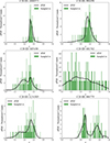 |
Fig. A.1. Redshift PDFs and sampled redshifts from MC process for 6 sources from 2 < z < 3 in our final sample (COSMOS2020 IDs: 1008373, 991850, 845430, 681762, 1231305, and 888775). The corresponding zPDFs from COSMOS2020 (Classic Catalog LePhare) are plotted in black while the selected redshifts from our MC process are shown in the green histograms (with the number of bins = the number of redshifts selected from 2 < z < 3 to better show each chosen redshift). Our 100 MC iterations accurately sample a variety of PDF shapes and capture secondary peaks. For C20 object #681762 (shown in the middle right panel), 6 chosen redshifts fall outside of 2 < z < 3 (which is expected as that PDF has portions outside 2 < z < 3). |
Companion statistics for our identified systems.
While increasing the number of MC iterations could improve our sampling the underlying zPDFs, this will not improve the recovery of true companion galaxies (i.e., it will not improve the overall recovered fraction nor improve the purity or completeness of identified companion galaxies). Satisfying the stringent line-of-sight criteria of Δv < 1000 km/s (or Δz ≲ 0.01) for companion galaxies is difficult, especially when both sources are photometric and need to simultaneously scatter to the ∼same redshift. When we examine the purity and completeness of identified companion galaxies within our 100 MC trials using the mock lightcone (see Section 3.4), we find that the average standard deviation in the purity is ∼0.9% and ∼0.3% for the completeness (these values are obtained by taking the average of the median σ of all 5 SzFs used for testing) and thus with 100 MC iterations we are well sampling the distributions of purity and completeness. With such little scatter in the recovered purity and completeness, increasing the number of MC iterations will not meaningfully change our results.
All Tables
All Figures
|
Fig. 1. Source breakdown as a function of redshift for objects in our final catalog based on the cuts detailed in Section 3.1. Sources from different methods are shown in different panels: wide field spectroscopic surveys (top left), targeted spectra (top right), and HST Hyperion (bottom left). Rather than including a histogram of photometric redshift counts, we include the photometric redshift fraction (i.e. the fraction of galaxies with only a photometric redshift measured) for reference on the bottom right. The location of Hyperion is included in each panel as a shaded gray region (2.4 < z < 2.7), and insets for this shaded region are included for the spectroscopic and grism redshift panels. Histograms with multiple survey sources are stacked. |
| In the text | |
|
Fig. 2. Galaxies in our final sample from 2 < z < 3 plotted in stellar mass and IRAC ch1 magnitude space (lower left) along with individual normalized histograms of stellar mass (top) and IRAC ch1 magnitude (lower right). All values are drawn from COSMOS2020 aside from the redshifts where we employ the best spectroscopic or grism redshift when available. For reference, our imposed IRAC ch1 magnitude cut is plotted as the dotted black line (note: some galaxies in our final sample lie above this line as our IRAC cut is an or cut on both ch1 and ch2). As expected, our spectroscopic and grism redshift sources (spec-z and grism-z, respectively) are primarily at brighter magnitudes and higher stellar masses in comparison to the distribution of photometric redshift only sources. Our final sample has a rough stellar mass limit of log(M*/M⊙)∼9.3 from 2 < z < 3 based on our imposed IRAC cuts. |
| In the text | |
|
Fig. 3. Spectroscopic completeness (or the fraction of sources with a spectroscopic and/or grism redshift, Fspec) as a function of IRAC ch1 magnitude for all sources from 2 < z < 3 in our final sample (purple) and a sub-sample of sources limited to the redshift range of Hyperion with tighter astrometric cuts (gold). Also included for reference are the underlying normalized IRAC ch1 magnitude distributions for each population along with the location of the imposed IRAC ch1 (or ch2) magnitude cut (vertical dashed black line). Spectroscopic completeness for both samples declines sharply as a function of magnitude. However, there is notably higher completeness for galaxies limited more closely to the bounds of Hyperion. |
| In the text | |
|
Fig. 4. Example of the distribution of galaxies in redshift and overdensity (σδ) space for one MC iteration used in this work (MC #82). Included are only those galaxies in the relevant redshift range for our fraction calculations (i.e., 2 < z < 3). Galaxies associated with Hyperion for this iteration are marked in red and field galaxies for this iteration are marked in blue. Unused galaxies for this iteration are marked in gray (which includes galaxies in the redshift range of Hyperion that are not associated with overdensity and galaxies in the field sample redshift range that are associated with other large structure, see Section 3.3.2). |
| In the text | |
|
Fig. 5. On-sky 2D view and 3D reconstruction of a potential galaxy companion for COSMOS2020 (C20) object #1006523 found during our MC process (MC iteration #87). The central galaxy (C20#1006523) is marked in gold with our 150 kpc search radius centered on that galaxy shown in green. The companion galaxy that meets both the projected separation and LoS velocity difference criteria is denoted in blue. Other nearby galaxies are shown in gray. While multiple galaxies fall within the projected separation criteria for this galaxy, the 3D LoS velocity difference cut helps isolate the single companion from other projected companions. |
| In the text | |
|
Fig. 6. Applied photometric redshifts (photo-zs) versus true simulation redshifts (zobs) for all galaxies in the Mock1 region of the simulated lightcone between 2 < zobs < 3. Galaxies that meet |Δz|< 0.15(1 + zobs) are marked in green (Hildebrandt et al. 2012). The statistics for these galaxies are listed in the upper right hand corner (outlier fraction, scatter, and bias, respectively). Photo-zs are applied to all galaxies in our simulated lightcone based on the observed photo-z statistics in COSMOS2020 as a function of magnitude and redshift. The scatter in photo-zs creates difficulty in recovering companion systems (see Section 3.4.1). |
| In the text | |
|
Fig. 7. Top: Median purity and median completeness of companion galaxies identified via the application of our MC methodology on the Mock1 lightcone at different levels of SzF. Bottom: Correction factor |
| In the text | |
|
Fig. 8. SzF for sources with a photo-z with 2 < z < 3 in our final sample in 20 × 20 bins of even RA and Dec (each bin is approximately ∼2.8′×3.0′). Over-plotted are the 2.5σδ and 4σδ contours of the massive structure defined as Hyperion in this work. As expected from the underlying spec-z surveys used in this study, we see increased SzF in the regions covered by the Hyperion overdensity finding a median SzF of ∼1.78 for Hyperion and a median SzF of ∼0.67 for the field. These median SzFs are used to determine the final correction factors applied to our uncorrected fckc values. |
| In the text | |
|
Fig. 9. Evolution of fckc and fckc-like measurements as a function of redshift. The values measured in this work are plotted in red with black borders with the star denoting our structure measurement and the circle denoting our field measurement. Other studies that examine merger and interaction rates in relation to overdensity or structure at relevant epochs have their results plotted similarly (i.e., structure or overdensity fraction as a star and field fraction as a circle, Hine et al. 2016; Monson et al. 2021; Liu et al. 2023; Shibuya et al. 2025) Various values from the literature that measure relevant major merger and pair fractions are also plotted for reference (Bundy et al. 2009; Conselice et al. 2009; de Ravel et al. 2009; Xu et al. 2012; López-Sanjuan et al. 2013; Tasca et al. 2014; López-Sanjuan et al. 2015; Ventou et al. 2017; Duncan et al. 2019; Romano et al. 2021; Duan et al. 2025), along with simulation predictions from Qu et al. (2017) and empirical fits from Romano et al. (2021) and Duan et al. (2025). Overall, we find that fckc evolves sharply at low redshift before peaking at z ∼ 4 with the measured fckc for Hyperion, though at lower redshift (z ∼ 2.5), existing above the peak value. Though some scatter exists, the existing measured merger and interaction rates for structures and overdensities are higher than the corresponding field rates at similar redshifts. |
| In the text | |
|
Fig. 10. Normalized distributions of projected separation (dproj; left), LoS velocity (ΔvLoS; center), and stellar mass ratio (right) between companion systems found in Hyperion (red) and the coeval field (blue). The plotted distributions contain all companion systems found over each of the 100 MC iterations used to identify close kinematic companions, so companion systems identified in multiple iterations are plotted multiple times. As opposed to the uniform and monotonic distributions seen for companion systems in the field, companion systems in Hyperion exhibit more complex distributions of dproj, ΔvLoS, and stellar mass ratio. |
| In the text | |
|
Fig. 11. Dependence of the Q (tidal strength) on Ri, p (the projected physical distance between companion and primary galaxy) for range of companion mass ratios considered in this work. The Q value contours are estimated using the typical size of a star-forming galaxy at z ∼ 2.5 from Ribeiro et al. (2016). Also included for reference are the |
| In the text | |
|
Fig. 12. ⟨Tmerge⟩ as a function of stellar mass. Contours represent the six different companion selection criteria and corresponding fitting coefficients from Kitzbichler & White (2008). These contours are all plotted at the median redshift of all pairs over all MC iterations (z ∼ 2.48). We also include the calculated ⟨Tmerge⟩ values for Hyperion (red) and the field (blue) at each of projected separation criteria employed (i.e., rproj ≤ 30 kpc (squares), 30 < rproj ≤ 50 kpc (diamonds), and 50 < rproj ≤ 150 kpc (crosses)). The ⟨Tmerge⟩ values calculated for Hyperion are shorter in each bin due to the larger stellar masses of galaxies in Hyperion companion systems. |
| In the text | |
|
Fig. A.1. Redshift PDFs and sampled redshifts from MC process for 6 sources from 2 < z < 3 in our final sample (COSMOS2020 IDs: 1008373, 991850, 845430, 681762, 1231305, and 888775). The corresponding zPDFs from COSMOS2020 (Classic Catalog LePhare) are plotted in black while the selected redshifts from our MC process are shown in the green histograms (with the number of bins = the number of redshifts selected from 2 < z < 3 to better show each chosen redshift). Our 100 MC iterations accurately sample a variety of PDF shapes and capture secondary peaks. For C20 object #681762 (shown in the middle right panel), 6 chosen redshifts fall outside of 2 < z < 3 (which is expected as that PDF has portions outside 2 < z < 3). |
| In the text | |
Current usage metrics show cumulative count of Article Views (full-text article views including HTML views, PDF and ePub downloads, according to the available data) and Abstracts Views on Vision4Press platform.
Data correspond to usage on the plateform after 2015. The current usage metrics is available 48-96 hours after online publication and is updated daily on week days.
Initial download of the metrics may take a while.