| Issue |
A&A
Volume 706, February 2026
|
|
|---|---|---|
| Article Number | A115 | |
| Number of page(s) | 17 | |
| Section | Astrophysical processes | |
| DOI | https://doi.org/10.1051/0004-6361/202554846 | |
| Published online | 04 February 2026 | |
Lighting up the nanohertz gravitational wave sky: Opportunities and challenges of multimessenger astronomy with pulsar timing array experiments
1
Dipartimento di Fisica “G. Occhialini” Università degli Studi di Milano-Bicocca Piazza della Scienza 3, I-20126 Milano, Italy
2
INFN, Sezione di Milano-Bicocca Piazza della Scienza 3, 20126 Milano, Italy
3
INAF – Osservatorio Astronomico di Brera via Brera 20 I-20121 Milano, Italy
4
INAF – Osservatorio Astronomico di Cagliari via della Scienza 5 09047 Selargius (CA), Italy
5
Como Lake Center for AstroPhysics, University of Insubria 22100 Como, Italy
6
Donostia International Physics Centre (DIPC) Paseo Manuel de Lardizabal 4 20018 Donostia-San Sebastian, Spain
7
IKERBASQUE, Basque Foundation for Science E-48013 Bilbao, Spain
★ Corresponding author: This email address is being protected from spambots. You need JavaScript enabled to view it.
Received:
28
March
2025
Accepted:
30
November
2025
Abstract
Pulsar timing array (PTA) experiments have the potential to unveil continuous gravitational wave (CGW) signals from individual low-redshift massive black hole binaries (MBHBs). Detecting these objects in both gravitational waves (GWs) and the electromagnetic (EM) spectrum will open a new chapter in multimessenger astronomy. We investigate the feasibility of conducting multimessenger studies by combining the CGW detections from an idealized 30 year Square Kilometer Array Mid telescope PTA and the optical data from the forthcoming Legacy Survey of Space and Time (LSST). To this end, we employed the L-Galaxies semi-analytical model applied to the Millennium simulation. We generated 200 different all-sky light cones that include galaxies, massive black holes, and MBHBs whose emission is consistently modeled based on their star formation histories and gas accretion physics. Our results predict an average of ≈33 CGW detections, with signal-to-noise ratios greater than five. The MBHBs associated with the detections are typically at z < 0.5, with masses of ∼ 3 × 10⁹ M⊙, mass ratios > 0.6, and eccentricities ≲0.2. In terms of EM counterparts, we find less than 15% of these systems to be connected with an active galactic nucleus detectable by LSST, while their host galaxies are easily detectable (< 23 mag) massive (M★ > 1011 M⊙) ellipticals with typical star formation rates (10−15 yr−1 < sSRF < 10−10 yr−1). Although the CGW-EM counterpart association is complicated by poor sky localization (only 35% of these CGWs are localized within 100 deg2), the number of galaxy host candidates can be considerably reduced (from thousands to several tens, depending on the CGW S/N) by applying priors based on the galaxy-MBH correlations. However, picking the actual host among these candidates is highly non-trivial, as they occupy a similar region in any optical color-color diagram. Our findings highlight the considerable challenges entailed in opening the low-frequency multimessenger GW sky.
Key words: gravitational waves / methods: numerical / galaxies: nuclei
© The Authors 2026
 Open Access article, published by EDP Sciences, under the terms of the Creative Commons Attribution License (https://creativecommons.org/licenses/by/4.0), which permits unrestricted use, distribution, and reproduction in any medium, provided the original work is properly cited.
This article is published in open access under the Subscribe to Open model. This email address is being protected from spambots. You need JavaScript enabled to view it. to support open access publication.
1. Introduction
The hierarchical assembly of structures and the presence of massive black holes (MBHs; mass M > 106 M⊙) lurking at the galactic centers hints at the existence of massive black hole binaries (MBHBs). As argued in Begelman et al. (1980), following a galaxy merger, the dynamical friction caused by stellar and gaseous components drags the MBHs of the interacting galaxies toward the nucleus of the newly formed system, enabling the formation of a gravitational bound MBHB at parsec separations (Milosavljević & Merritt 2001; Yu 2002; Mayer et al. 2007; Fiacconi et al. 2013; Bortolas et al. 2020, 2022; Li et al. 2022). Beyond this point, the system keeps shrinking through interaction with individual stars at the galactic center (Quinlan & Hernquist 1997; Sesana et al. 2006; Vasiliev et al. 2014; Sesana & Khan 2015) and/or torques extracted from a circumbinary gaseous disk (Escala et al. 2004; Dotti et al. 2007; Cuadra et al. 2009; Bonetti et al. 2020; Franchini et al. 2021, 2022). These processes are relevant down to milli-parsec separations when the emission of gravitational waves (GWs) becomes the main process of extracting energy and angular momentum from the system, which in turn drives the MBHB to coalescence on timescales between megayears and several gigayears.
Massive black hole binaries with M > 108 M⊙ placed at low redshifts are loud GW sources at nanohertz frequencies (10−9 − 10−7 Hz). This window is currently being probed by pulsar timing array (PTA) experiments through monitoring of the spatially correlated fluctuations in the arrival time of radio pulses from a network of galactic millisecond pulsars (Foster & Backer 1990). There are six different PTA collaborations taking data: the European Pulsar Timing Array (EPTA; Kramer & Champion 2013; Desvignes et al. 2016), the North American Nanohertz Observatory for Gravitational Waves (NANOGrav; McLaughlin 2013; Arzoumanian et al. 2015), the Parkes Pulsar Timing Array (PPTA; Manchester et al. 2013; Reardon et al. 2016), the Indian PTA (InPTA; Susobhanan et al. 2021), the Chinese PTA (CPTA; Lee et al. 2016), and the MeerKAT PTA (MPTA; Miles et al. 2023). All of them have recently reported evidence of a stochastic GW background (sGWB) with amplitude [1.7 − 7] × 10−15 at 1 yr−1 frequency, compatible with the existence of a cosmic MBHB population (EPTA Collaboration and InPTA Collaboration 2023a; Agazie et al. 2023; Reardon et al. 2023; Xu et al. 2023; Miles et al. 2025).
In addition to the eventual detection of the nanohertz sGWB, PTA collaborations also aim to uncover continous GW (CGW) sources, i.e., GWs from individual MBHBs whose deterministic signals can be separated from the sGWB (Sesana et al. 2009; Babak & Sesana 2012; Ravi et al. 2015; Kelley et al. 2018; Falxa et al. 2023). Systematic CGW searches in simulated MBHB populations have shown that PTAs will predominantly select systems > 109 M⊙ at low-z (z < 0.5) emitting GWs at ∼ 108 Hz (Rosado et al. 2015; Kelley et al. 2018; Truant et al. 2025). The abundance of these detections seems to be moderately sensitive to binary evolution parameters such as environmental coupling or MBHB eccentricity (Kelley et al. 2018; Gardiner et al. 2023). For instance, Truant et al. (2025) have demonstrated that the number of sources detectable by PTAs with long observing baselines increases as the eccentricity of the underlying MBHB population rises. The noise characteristics of the PTA also appear to impact CGW detections. As indicated by Cella et al. (2025), PTAs with a large white noise (> 300 ns) will hamper the detection of light MBHBs (≲ 109 M⊙).
The detection of a single MBHB can be complemented with multimessenger studies. These require the electromagnetic (EM) identification of the active galactic nucleus (AGN) or galaxy associated with the CGW. This task is especially challenging for PTAs given their poor sky-localization capabilities (a few to thousands of deg2, depending on S/N, Sesana & Vecchio 2010) and the impossibility, in most cases, of directly constraining the source redshift due to the lack of MBHB frequency evolution within the observing time. There are typically several millions of potential hosts within the localization error box, making the identification of peculiar features associated with the presence of the binary vital for narrowing down the pool of candidates. For example, different studies have shown that CGWs tend to be hosted in massive galaxies (∼ 1011 M⊙) brighter and redder than the overall massive galaxy population (Rosado & Sesana 2014; Simon et al. 2014; Mingarelli et al. 2017; Cella et al. 2025). Apart from studying peculiar features, the physical dependence of the CGW amplitude on the MBHB chirp mass and distance to the observer can be coupled with MBH mass-host galaxy correlations in order to assign to each galaxy a probability of being the actual host. This approach was first introduced by Goldstein et al. (2019), who demonstrated that there is a 90% probability that the true host is among the 0.01% more massive nearby galaxies within the localization error box (usually a few tens to a few thousands of massive ellipticals; see also Petrov et al. 2024).
While multimessenger studies may be feasible with PTAs, there are still important caveats to address. First, most of the pipelines used to detect the hosts of CGWs have been calibrated using galaxy catalogs complete up to z ∼ 0.1 (Arzoumanian et al. 2021; Petrov et al. 2024). However, different studies indicate that resolvable CGWs can also be found at higher redshifts (z ∼ 0.5, Rosado et al. 2015), thus dramatically increasing the number of galaxies within the error box. Second, it is unclear whether the MBHBs detected by PTAs will be associated with an AGN emission (Burke-Spolaor 2013; Charisi et al. 2016, 2018). This latter point is particularly important, as the lower abundance of AGNs with respect to galaxies would help narrow down the number of candidates (Tanaka et al. 2012). In this paper we systematically address these points by means of realistic simulations of the GW and EM sky obtained with the L-Galaxies semi-analytical model (SAM; Izquierdo-Villalba et al. 2022). The simulations are used to construct synthetic full-sky light cones populated with realistic galaxies, MBHs, and MBHBs. From those, we compute the nanohertz GW signal and identify the MBHBs sourcing CGWs that can be resolved by an Square Kilometer Array Mid telescope (SKA)-like PTA. We characterize their AGN emission and study the properties of their host galaxies. We then make use of the Fisher matrix calculations developed by Truant et al. (2025) to compute the sky localization error of each CGW and employ the methodology of Goldstein et al. (2019) to narrow down the number of galaxy host candidates inside this area. We contrast the properties of these candidates with those of the true hosts in search of distinctive signatures that might facilitate the CGW-EM counterpart association. This allows us to make a realistic assessment about the feasibility and challenges entailed in the pursuit of multimessenger astornomy in the nanohertz GW band.
The paper is structured as follows. Section 2 presents the L-Galaxies SAM and the methodology used to generate the used light cones. In Section 3 we describe the approach used to generate synthetic photometry of galaxies, MBHs, and MBHBs. In Sect. 4 we outline the characteristics of the PTA used and describe the methodology for detecting CGWs, including how to identify their parameters. Section 5 shows the methodology used to define the sky-localization area and reduce the number of potential host candidates. We present our results in Section 6, focusing on the properties of the CGW hosts, their AGN counterpart, and the possibility of identifying them in the sky. We summarize our main findings in Section 7. A Lambda cold dark matter cosmology with parameters Ωm = 0.315, ΩΛ = 0.685, Ωb = 0.045, σ8 = 0.9, and h = H0/100 = 67.3/100 km s−1 Mpc−1 is adopted throughout the paper (Planck Collaboration XVI 2014).
2. The virtual universe: A nanohertz light cone
To create the population of galaxies, MBHs and MBHBs used in this work, we employ L-Galaxies, a state-of-the-art SAM calibrated to reproduce a vast array of observational properties such as the galaxy stellar mass function, the cosmic star formation rate density, galaxy colors and the fraction of passive galaxies (Henriques et al. 2015, 2020; Yates et al. 2021). In particular, we make use of L-Galaxies in the version presented in Izquierdo-Villalba et al. (2022) whose modifications improve the physics of MBHs (formation and growth), introduce the formation and dynamical evolution of MBHBs and allow the creation of light cones. In the following, we briefly summarize the main features of the model.
2.1. Dark matter and baryons
The L-Galaxies SAM is built on the subhalo (hereafter just halo) merger trees extracted from N-body dark matter simulations. In particular, L-Galaxies has been tested on the Millennium and TNG-DARK suit of simulations (Guo et al. 2011; Henriques et al. 2015; Ayromlou et al. 2021). Here, we make use of the merger trees from the Millennium-I (MS; Springel et al. 2005), whose minimum particle mass and large cosmological volume allow us to trace the build-up of halos of a wide range of masses. Specifically, MS follows the cosmological evolution of 21603 DM particles of mass 8.6 × 10⁸ M⊙/h inside a periodic box of 500 Mpc/h on a side, from z = 127 to the present. Particle data of MS was stored at 63 different times or snapshots. Structures formed in these outputs were identified by applying the friend-of-fried and SUBFIND algorithms and linked across time as progenitors and descendants in the so-called merger tree via the L-HALOTREE code (Springel et al. 2001). Finally, given the coarse resolution of the DM outputs, L-Galaxies performs an internal time interpolation (∼ 5−50 Myr, depending on redshift) to improve the tracing of the baryonics physics involved in the assembly of galaxies, MBHs, and MBHBs. Concerning the cosmology, originally MS was run with the WMAP1 & 2dFGRS concordance cosmological parameters. However, the version of the merger trees used here is re-scaled with the procedure of Angulo & White (2010) to match the cosmological parameters provided by Planck first-year data (Planck Collaboration XVI 2014).
The evolution of galaxies is traced by L-Galaxies using a sophisticated galaxy formation model able to trace the evolution of the gas and stellar component of structures formed along the mass assembly of DM merger trees. As soon as a DM halo is resolved in the merger tree, L-Galaxies assigns a brayon fraction to it, consistent with the cosmological baryon fraction (White & Frenk 1991). These baryons are initially distributed in a quasi-static hot gas atmosphere which progressively cools down at a rate given by the halo dynamical time. This cooled gas inherits the specific angular momentum from its host DM halo and settles at its center in the form of a disk-like structure. The continuous fuel of cold gas raises the mass of the cold disk triggering star formation events and leading to the assembly of a stellar component distributed in a disk (Croton et al. 2006). The results of this star formation process cause short-lived and massive stars to explode as supernovae, injecting energy and metals into the cold gas disk, heating it and eventually pushing it beyond the virial radius of the DM halo (Guo et al. 2011). The cold gas component is also regulated by the radio-mode feedback of the central MBH, which efficiently reduces or even suppresses cooling flows in massive halos (Croton et al. 2006; Croton 2006). Thanks to the continuous star formation, galaxies can develop massive stellar discs that can be prone to non-axisymmetric instabilities (the so-called disk instabilities) which lead to the formation of a central ellipsoidal component called pseudobulge.
Besides internal processes, galaxies interact among themselves, as a result of the hierarchical growth of DM halos. The time scale of these interactions is given by the dynamical friction experienced by the merging galaxies, accounted for by using the Binney & Tremaine (2008) formalism. The outcome of the interaction depends on the baryonic mass ratio (mR) of the two interacting systems. For large mass ratios (mR > 0.2, major mergers), the interaction destroys the discs of the two galaxies and leads to the formation of pure spheroidal component (elliptical galaxy) whose mass increases as a consequence of a collisional burst (Henriques et al. 2015). Conversely, small mass ratios (mR < 0.2, minor mergers) allow the survival of the most massive galaxy disk component (which undergoes a burst of star formation) and its bulge grows as a consequence of the integration for the entire stellar mass of the satellite galaxy (forming a classical bulge). Besides these two merger types, the version of L-Galaxies used in this work includes a prescription for smooth accretion to deal with the physics of extreme minor mergers (see for more details Izquierdo-Villalba et al. 2019b). Finally, L-Galaxies also models large-scale effects such as ram pressure stripping or galaxy tidal disruption (Henriques et al. 2015).
2.2. Massive black holes
L-Galaxies includes a comprehensive physical model to follow the formation of the first MBHs (Spinoso et al. 2023). It tracks the spatial variation of the Lyman Werner radiation and metals to track the formation of massive (direct collapse) and intermediate-mass (collapse of dense, nuclear stellar clusters) seeds. A sub-grid approach also accounts for the formation of light seeds. This model can only be used when the resolution of the DM merger trees reaches the small halos (< 108.5 M⊙)1 where the genesis of the first MBHs take place. Given the characteristics of the MS simulation, newly resolved DM halos are found as soon as their masses reach 1010 M⊙/h. This hinders the possibility of using the self-consistent seeding model included in L-Galaxies. Since we are interested here in massive, nearby MBHBs, this is not a limitation, because the early growth of MBHs tends to erase the signatures of the seed population. Taking into account the above, when any DM halo is firstly detected in the MS merger trees, L-Galaxies places an MBH seed of initial mass 104 M⊙ and spin, χ, extracted randomly form a uniform distribution ranging between 0 < χ < 0.98. After the seeding, the MBH can grow through three different mechanisms: cold gas accretion, hot gas accretion and mergers with other MBHs. In the following paragraphs, we outline the main characteristics and the default values of free parameters employed in the “Fiducial” model (see also Izquierdo-Villalba et al. 2020, 2022).
-
Cold gas accretion: This mechanism is the main growth channel and it is activated by two processes (see Section 2.1):
-
Galaxy mergers: MBHs can accrete a part of the cold gas component of the galaxy given by
 (1)
(1)where mR < 1 is the ratio between the baryonic mass content of the two interacting galaxies, V200 is the viral velocity of the dark matter halo hosting the interacting galaxies, zmerger is the redshift at with the merger take place, Mgas is the cold gas content of the host galaxy. VBH and
 are two adjustable parameters set to VBH = 280 km/s and 0.025, respectively.
 -
disk instabilities: The gas accreted by any MBH after any instability is given by
 (2)
(2)where
 similarly to a
  is a free parameter that describes the efficiency of the accretion process and it set
  and zDI is the redshift at which the disk instability occurs. Finally,
  is the amount of stars triggering the disk instability. L-Galaxies assumes that the cold gas mass available for accretion after mergers or disk instabilities is not instantaneously accreted. Instead, it is stored in a gas reservoir around the MBH and progressively consumed according to a first phase of Eddington-limited growth followed by a decaying sub-Eddington phase (see the results of Bonoli et al. 2009; Hopkins & Quataert 2010). While this work does not utilize them, we emphasize that the latest modifications of L-Galaxies allow for the possibility that some MBHs undergo episodic super-Eddington accretion episodes (Izquierdo-Villalba et al. 2024). In future works, we will investigate how incorporating these events could impact the detection prospects of CGWs.
-
-
Hot gas accretion: MBHs are fueled by the constant inflow of hot gas that surrounds the galaxy. This hot accretion mode is characterized by a small accretion rate given by (Henriques et al. 2015)
 (3)
(3)where Mhot is the total mass of hot gas surrounding the galaxy and kAGN is a free parameter chosen to reproduce the galaxy luminosity function set to 3.5 × 10⁻³ M⊙/yr. Despite being a constant process, the accretion flow in this regime is orders of magnitude smaller than the MBH Eddington limit and the growth of the MBH is minimal.
2.3. Massive black hole binaries
On top of the evolution of single MBH, L-Galaxies includes analytical prescriptions to deal with the formation and dynamical evolution of MBHBs (Izquierdo-Villalba et al. 2022). Following the seminal work by Begelman et al. (1980), L-Galaxies follows the evolution of these systems in different stages: pairing and hardening & gravitational wave phase. The first one starts after a galaxy merger. During this phase, the dynamical friction caused by the stellar component of the remnant galaxy reduces the initial separation (∼kpc) between the nuclear and the satellite MBHs, moving the latter toward the galactic center. The time spent by the satellite MBH in this phase is set according to the expression of Binney & Tremaine (2008). Once the satellite MBH reaches the galactic nucleus, it binds gravitationally with the central MBH (∼pc separation) and the hardening & GW phase starts. From hereafter, it is assumed that the most massive black hole in the system is the primary one (with mass MBH, 1) whereas the less massive one is tagged as the secondary (with mass MBH, 2). The initial eccentricity of the binary system, e0, is chosen randomly between [0 − 1] and the initial separation, a0, is selected to be the scale at which MBulge(< a0) = 2 MBH, 2, where MBulge(< a0) corresponds to the mass in stars of the hosting bulge within a0. To compute the value of a0, L-Galaxies assumes that the bulge mass density profile follows a Sérsic model (Sersic 1968). During this hardening & GW phase, the separation (aBH) and eccentricity (eBH) of the binary system are evolved depending on the environment in which the MBHB is embedded. If the gas reservoir around the binary is larger than its total mass, the evolution of the system is driven by the interaction with a circumbinary gaseous disk and then GWs emission (Peters & Mathews 1963; Dotti et al. 2015; Bonetti et al. 2019). Otherwise, the system evolves via the interaction with single stars embedded in a Sérsic profile and the emission of GWs (Peters & Mathews 1963; Quinlan & Hernquist 1997; Sesana et al. 2006). In some cases, the lifetime of an MBHB can be long enough that a third MBH can reach the galaxy nucleus and interact with the binary system. In this scenario, the final stage of the MBHB (prompt merger of the MBHB or the ejection of the lightest object) is determined using the probability distributions presented in Bonetti et al. (2018).
Finally, L-Galaxies follows the growth of MBHBs in a different way than the one of single MBHs. In particular, the code assumes that the accretion rates of the two SMBHs of the binary are correlated, as proposed by Duffell et al. (2020):
 (4)
(4)
where  and
and  are respectively the accretion rate of the primary and secondary MBHs and q = MBH, 2/MBH, 1 the binary mass ratio. For simplicity, the latter is set by L-Galaxies to the Eddington limit. Notice that if the cold gas reservoir is depleted, the secondary MBH is not able to accrete anymore. However, the primary MBH is still able to consume matter from the hot gas mode of Eq. (3).
2.4. The Fiducial and Boosted models
The work of Izquierdo-Villalba et al. (2022) showed that the Fiducial model described above ( and
and  ) gives rise to a population of MBHs in agreement with current observational constraints (quasar luminosity functions and black hole mass functions), but the resulting MBHB population produces an sGWB of
  , which is in mild tension with recent PTA observations, although in agreement with most of the theoretical predictions in literature. To address this discrepancy, the authors explored a Boosted model in which the two phases of growth during cold gas accretion were untouched, but the gas accretion efficiency during mergers was raised up to
  . The results showed that this model was able to generate an sGWB amplitude
 ![Mathematical equation: $ A_\mathrm{{yr}^{-1}}\,{\in}\,\left[1.9{-} 2.6 \right]\,{\times}\,10^{-15} $](/articles/aa/full_html/2026/02/aa54846-25/aa54846-25-eq16.gif) in better agreement with the latest PTA results (Agazie et al. 2023; EPTA Collaboration and InPTA Collaboration 2023a; Reardon et al. 2023; Xu et al. 2023). In this work, we make use of both the Fiducial and Boosted models.
in better agreement with the latest PTA results (Agazie et al. 2023; EPTA Collaboration and InPTA Collaboration 2023a; Reardon et al. 2023; Xu et al. 2023). In this work, we make use of both the Fiducial and Boosted models.
2.5. The simulated light cones: Massive black hole binary population selection
To make a more direct comparison with observations and build sky-localization areas, we need to create full-sky light cones from the L-Galaxies outputs. To transform the discrete number of comoving boxes generated by L-Galaxies into a full-sky light cone we use the method presented in Izquierdo-Villalba et al. (2019a). In brief, the methodology takes the comoving boxes of galaxies created at different cosmological times and replicate them 𝒩 times in each Cartesian coordinate. The value of 𝒩 is set in such a way that the last replica displays a comoving distance from the observer as large as the desired redshift depth. The observer is placed in a position inside the first replica of the box (typically the first corner), and each galaxy is placed inside the light cone by making use of the box replica which satisfies the condition that the galaxy crosses the observer past light cone. For this work, we only keep the galaxies within the light cone whose stellar mass M∗ > 1010.3 M⊙. We have checked that this cut does not affect the predictions about the sGWB but it improves the handling of the L-Galaxies outputs. To show the outcome of this procedure, the bottom panel of Fig. 1 presents a slice of one of the full-sky light cone used in this work.
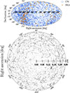 |
Fig. 1. Upper panel: Sky distribution of the SKA PTA pulsars (orange) and the MBHBs detected as CGW (blue) within the 200 MBHB realizations. The size of the blue points corresponds to the S/N of the CGW. Lower panel: Right ascension versus redshift for all the galaxies placed in the light cone within a thin slide of 0.1 deg. For the sake of clarity, we only show the z < 0.3 redshift range. |
We generated a total of ten different light cones: five using the Fidicual model and five employing the Boosted one. Since the observer plays an important role in determining which galaxies enter inside the light cone, each light cone was constructed assuming a different position of the observer in the simulation box. Specifically, the observer was placed in the following random positions: {xObs, yObs, zObs}={0, 0, 0} Lbox; {0.25, 0.96, 0.40} Lbox; {0.36, 0.30, 0.76} Lbox; {0.52, 0.46, 0.82} Lbox; and {0.74, 0.45, 0.10} Lbox, where Lbox corresponds to the box size of the MS simulation. For each of these ten light cones, we created 20 realizations, slightly changing the population of MBHBs. The first ten were generated drawing ten random polarization and inclination of each merging MBHB inside the light cone. The other ten were built by re-drawing each time the total mass of the MBHB according to the Mstellar − MBH relation predicted by the light cone at the redshift in which the binary is placed. In particular, the total mass was assigned randomly between the 10-90 percentile of the scaling relation and the mass of the primary and secondary MBH is assigned by keeping the mass ratio predicted by L-Galaxies. Considering all the variants, we created a total population of 200 merging MBHBs.
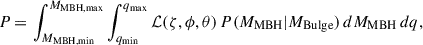
To pitch the most realistic scenario, among the 200 MBHB populations, we selected those consistent with the latest results presented by the EPTA collaboration (EPTA Collaboration and InPTA Collaboration 2023a). Given that the most constraining evidence of nanoHz gravitational waves comes from the lowest frequency bin probed by the array, f = 1/10 yr−1 (f1/10yr), we retained only the MBHB populations predicting an sGWB amplitude that fall within 3σ of the observed posterior distribution. The distribution of the sGWB amplitude at f1/10yr reported by EPTA and the L-Galaxies MBHB population is presented in Fig. 2. As shown, the generated populations are consistent with observational constraints within 3σ confidence level. Despite this, we stress that the characteristic strain produced by the generated MBHB population peaks at slightly lower values.
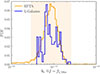 |
Fig. 2. Normalized distribution of the sGWB characteristic strain amplitude at f1/10yr. The orange histogram represents the posterior distribution inferred by the EPTA collaboration (EPTA Collaboration and InPTA Collaboration 2023a), while the orange shaded region represents the ±3σ interval. The blue histogram corresponds to the strains produced by the MBHB population generated by L-Galaxies. |
3. The optical counterpart of galaxies and MBH(B)s
Since we are interested in the optical identification of the CGW hosts, in this section we outline the procedure for computing the photometry of the galaxy stellar component and accreting an MBHs or MBHBs. Notice that the final photometry of the galaxy will be the sum of these two contributions. Among all the optical surveys, we focus on the Vera C. Rubin Observatory’s Legacy Survey of Space and Time (LSST; Ivezić et al. 2019), whose observing strategy will enable the detection of very dim and high-z objects across half of the sky. Specifically, the deep-observing mode of LSST will perform observations in the u, g, r, i, z filters2 with limiting magnitudes corresponds to u ∼ 26.1, g ∼ 27.4, r ∼ 27.5, i ∼ 26.8 and z ∼ 26.1 (LSST Science Collaboration 2009).
3.1. The galaxy photometry: Stellar population synthesis
The galaxy magnitude in the u, g, r, i, z filters is computed self-consistently by L-Galaxies using a simple stellar population synthesis model (SSP) combined with dust-reddening. In short, within a given filter system L-Galaxies creates tabulated grids of the observed luminosity generated by an SSP of fixed mass but different stellar ages and metallicities. Combining these grids with the star formation history of the galaxy and dust attenuation (due to the interstellar medium and molecular clouds) enables the computation of the observed photometry of a galaxy at any redshift. For further information, we refer to Guo et al. (2011) and Henriques et al. (2015). The typical photometry predicted by L-Galaxies for massive galaxies (M∗ > 1011 M⊙) at low-z is shown in the upper panels of Fig. 3, which make clear that these galaxies can be up to two times brighter in the reddest filters. Finally, we stress that the version of the model used here is tuned to reproduce the fraction of passive galaxies at z < 3 and the galaxy colors in the Sloan Digital Sky Survey optical bands (see Henriques et al. 2015).
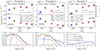 |
Fig. 3. Upper and middle panels: Observed photometry in LSST for three detected MBHBs (upper panels) and the stellar component of their host galaxies (middle panels). Blue, green, red, purple, and brown dots correspond to the flux inside the u, g, r, i, z filters, respectively. The properties of the binary and the host galaxy are indicated in each panel. Lower panels: Observed SED ( |

3.2. The active galactic nucleus photometry: Accreting MBHs and MBHBs
The version of L-Galaxies used in this work does not include any model to compute the photometry of the AGN associated with an accreting MBH. Thus, to determine the magnitude of these objects in a given generic filter “j” we need to determine its spectral energy distribution (SED). In particular, the magnitude (mj) is determined by
 (5)
(5)
where ![Mathematical equation: $ L_{\nu}^\mathrm{{obs}}(\lambda) \, [\rm{erg\, s}^{-1} \, Hz^{-1}] $](/articles/aa/full_html/2026/02/aa54846-25/aa54846-25-eq19.gif) is the observed SED of the source3 at the observed wavelength λ, DL the source luminosity distance, Tj(λ) the transition curve of the “j” filter and λmin and λmax the minimum and maximum wavelength covered by it. Taking into account this, in the upcoming sections we describe the approach used to associate an SED to each accreting MBH/MBHB taking into account the accretion properties of the system.
is the observed SED of the source3 at the observed wavelength λ, DL the source luminosity distance, Tj(λ) the transition curve of the “j” filter and λmin and λmax the minimum and maximum wavelength covered by it. Taking into account this, in the upcoming sections we describe the approach used to associate an SED to each accreting MBH/MBHB taking into account the accretion properties of the system.
3.2.1. The spectral energy distribution of MBHBs
Different hydrodynamical simulations have demonstrated that gas around MBHBs settles in the form of a circumbinary disk (see e.g. Ivanov et al. 1999; Haiman et al. 2009; Lodato et al. 2009). Besides this, it has been shown that the gravitational torque exerted by MBHB is capable of opening a large cavity around the MBHB, with gas streams flowing inside and leading to the formation of mini-discs structures around each MBH (Ragusa et al. 2016; Fontecilla et al. 2017; Franchini et al. 2023). Considering this gas structure, the total rest-frame SED of an MBHB, Lν, can be characterized by
 (6)
(6)
where  is the emission generated by the mini-disk of the primary (i = 1) and secondary (i = 2) MBH,
  is the one originated by the circumbinary disk, and
  is the radiation coming from a non-thermal corona. In the following paragraphs, we outline the procedure used to compute each component of Eq. (6). We stress that we did not model any infrared emission coming from a torus structure surrounding the MBHB. Furthermore, we do not account for any obscuration in the emission of AGNs caused by gas and dust in the galaxy’s interstellar medium. Therefore, the SEDs and photometry of AGNs derived in this work should be regarded as the optimal observing scenario.
3.2.1.1. Circumbinary disk:
The spectral emission radiated by the structure is computed according to the thin disk model (Shakura & Sunyaev 1973):
 (7)
(7)
where kB is the Boltzmann constant, h is the Planck constant, c is the speed of light, and ν is the rest-frame frequency. The variable x is defined as x ≡ r/rSchw, with r being the radial distance to the MBH and rSchw the Schwarzshild radius. The temperature of the circumbinary disk at a given distance x, T(x), is determined by
![Mathematical equation: $$ \begin{aligned} T(x) \,{=}\, \left[ \frac{3\dot{M}_{\rm {BH}}c^6}{64\pi \sigma _{\rm {B}} G^2 M^{2}_{\rm {BH}}} \right]^{\frac{1}{4}} \left[ \frac{1}{x^{3}} \left(1 - \sqrt{\frac{3}{x}}\right)\right]^{\frac{1}{4}}, \end{aligned} $$](/articles/aa/full_html/2026/02/aa54846-25/aa54846-25-eq25.gif) (8)
(8)
where G is the gravitational constant and σB is the Stefan-Boltzmann constant. In this case, MBH = MBH, 1 + MBH, 2, where MBH, 1 (MBH, 2) is the mass of the primary (secondary) MBH. Similarly, ṀBH = ṀBH,1+ ṀBH,2, where ṀBH,1 (ṀBH,2) corresponds to the accretion rate onto the primary (secondary) MBH. Finally, (xin,xout) = (2 aBHB/rSchw,10 aBHB/rSchw), where aBHB is the binary semi-major axis (see similar integration approach in Cocchiararo et al. 2024).
3.2.1.2. Mini-disk:
The emission raised from the mini-disk structures is going to be modeled differently according to the value of fEdd = Lbol/LEdd, predicted by L-Galaxies. Specifically, if fEdd > 0.03 the accretion flow around the MBH can be considered as a thin disk (see Eq. (7)). On the contrary, the accretion was modeled according to an advection-dominated accretion flow where the gas is stored in an optically thin and geometrically thick disk. In the following, we describe the equations used to determine the emission of these structures.
-
Thin disk accretion flow: We followed the modeling of Eq. (7) where the integration is performed from xin = 3 to xout = min(3000,rHill/rSchw). rHill corresponds to the Hill radius and accounts for the fact that the presence of a massive companion can truncate the extension of an MBH mini-disk (see a similar approach in Kelley et al. 2019). Here, we defined rHill as
 (9)
(9)The term MBH, i is the mass of the primary (i = 1) or secondary (i = 2) MBH, and MBHB is the total mass of the binary. We stress that for the sake of simplicity, Eq. (9) ignores the eccentricity of the binary system. As we show in Section 6, we do not expect that this simplification affects our results since the targeted sample features a low eccentricity.
-
Advection-dominated accretion flow: We closely followed the work of Mahadevan (1997), which showed that the SED of an advection-dominated accretion flow (ADAF) process is the result of three physical processes: synchrotron radiation (
 ), inverse Compton scattering (
 ), and bremsstrahlung radiation (
 ):
): (10)
(10)The expression of each component is formulated as


where mi = ṀBH,i/ṀEdd,i is the accretion rate of the i MBH in units of Eddington accretion, we set α = 0.3, β = 0.5, δ = 2000−1, νp is the frequency at which the synchrotron radiation is maximum, Te is the electron temperature, rmin = 3 rSchw, rmax = 103 rSchw and s1, s2, s3, 𝒜 are constants. For the sake of brevity, we refer to Mahadevan (1997) for the specific values and computations of the parameters.
-
Non-thermal corona: We assumed that the non-thermal emission produces a spectrum according to (Regan et al. 2019; Cocchiararo et al. 2024):
 (11)
(11)where τ = − 1.7, νc = 7.2 × 10¹⁹ Hz and
 (12)
(12)where ν0 = 4.8 × 10¹⁶ Hz and νf = 2.4 × 10¹⁸ Hz. The value of LX-ray is the sum of the emission produced by each MBH in the hard X-rays (2-10 KeV), computed after applying the corrections of Shen et al. (2020) to the total bolometric luminosity of the MBHB.
To show the potential of our methodology, in Fig. 3 we present the SED and LSST photometry of three MBHBs inside our light cones. As expected, the ones accreting during the thin disk regimen exhibit a predominantly blue SED, resulting in brighter photometry in the u and g filters. On the contrary, the MBHB accreting in the ADAF mode features a dominant red SED and photometry. Taking into account the above model and the MBH/MBHB accretion physics included in L-Galaxies (Section 2.2 and Section 2.3), there are three possible SED combinations assigned to our MBHBs. The first case occurs when the two MBHs in the binary accrete in the thin disk regime, being very common in binaries with similar mass ratios (see the middle/lower left panel of Fig. 3). The second case happens when the secondary MBH lies in the thin disk regime (always set by default at the Eddington limit) but the primary undergoes ADAF accretion (see the middle/lower center panel of Fig. 3). This case is common for very unequal mass systems. Finally, in the third scenario the secondary is not accreting while the primary is in the ADAF accretion mode due to hot gas accretion (see the middle/lower right panel of Fig. 3).
3.2.2. The spectral energy distribution of MBH
In the case of single MBHs, we employ the same formalism presented in the previous section. Specifically, Eq. (7) (thin disk) and Eq. (10) (ADAF). The main difference is the absence of a circumbinary disk and the transformation of the mini-disk around the MBH into a regular accretion disk with no truncation at the Hill’s radius.
4. Detecting continuous gravitational wave sources
In this section, we summarize the methodology used to detect eccentric MBHBs using an idealized SKA PTA experiment with 30 years of observations. For the sake of brevity, we only refer to the main equations employed in this work. For a detailed computation of the procedure, we refer to Truant et al. (2025).
4.1. Signal-to-noise computation, parameter estimation and noise modeling
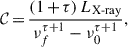
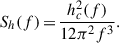
To determine the possibility of detecting the signal of an MBHB in the nHz regime, it is necessary to compute the signal-to-noise ratio. Assuming that a CGW is present in the timing residual of a pulsar, the S/N can be computed as
 (13)
(13)
Here, SK(f) is the noise power spectral density (NPSD) and  represents the time residuals in the frequency domain. Following Truant et al. (2025), the S/N for a generic eccentric MBHB detected with an array of pulsars (NPulsars) can be expressed as
![Mathematical equation: $$ \begin{aligned} \left(\dfrac{S}{N}\right)^2_{\rm {tot}}\,{=}\, \sum _{p = 1}^{N_{\rm {Pulsar}}} \left[\sum _{n = 1}^{\infty } \dfrac{2}{S_{k,p}(f_n)} \int _{t_0}^t dt^{\prime }\, s_{n,p}^2(t^{\prime })\right], \end{aligned} $$](/articles/aa/full_html/2026/02/aa54846-25/aa54846-25-eq38.gif) (14)
(14)
where Sk, p(fn) and sn, p(t′) correspond to the NPSD and the time residuals of the p pulsar.
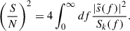
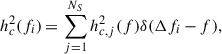
In the case of high S/N, the MBHB parameters can be estimated through the computation of the Fisher information matrix (Γ)4. Specifically, we considered nine free parameters:
 (15)
(15)
We note that ζ is the GW amplitude given ζ = (Gℳz)5/3/c4DL, where ℳz the redshifted chirp mass, DL is the luminosity distance, G is the gravitational constant, and c is the light speed. The term fk represents the orbital angular frequency, e is the binary eccentricity, ι is the inclination angle, ψ is the polarization angle, l0 is the initial phase of orbit, and γ is the direction of the pericenter with respect to 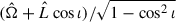 , where
  and
and  correspond to the orbital angular momentum and GW propagation direction, respectively. Finally, (θ,ϕ) = π/2 − Dec,RA), where Dec is the declination and RA is the right ascension. Following Truant et al. (2025), the Fisher information matrix of a generic eccentric binary can be re-written as
![Mathematical equation: $$ \begin{aligned} \Gamma _{ij} \,{\simeq }\, \sum _{p = 1}^{N_{\rm {Pulsar}}} \left[\sum _{n = 1}^{\infty } \dfrac{2}{S_{k,p}(f_n)} \int _{t_0}^{t} dt^{\prime } \, \partial _i s_{n,p}(t^{\prime }) \partial _j s_{n,p}(t^{\prime })\right], \end{aligned} $$](/articles/aa/full_html/2026/02/aa54846-25/aa54846-25-eq43.gif) (16)
(16)
where ∂i and ∂j are the partial derivatives of time residual in the frequency domain, s(f), with respect to the λi and λj parameters, respectively. Notice that the covariance matrix is simply the inverse of the Fisher information matrix (Γ−1). Therefore, the elements on the diagonal correspond to the parameter variance ( ), while the off-diagonal terms represent the correlation coefficients between parameters (
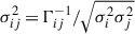 ).
).
Finally, the pulsar NPSD could be characterized by splitting it into two separate terms:
 (17)
(17)
In the equation, the term Sp(f) encapsulates all noise sources related to the telescope sensitivity or intrinsic noise in the pulsar emission mechanism (among many others). It is usually described as a combination of three terms:
 (18)
(18)
Here, Sw accounts for stochastic errors in the measurement of a pulsar arrival time and is modeled as Sw = 2Δtcadσw2. The value of Δtcad corresponds to the observation cadence and σw is determined in such a way that the pulse irregularity is a random Gaussian process described by the root mean square value σw. The terms Sred(f) and SDM(f) are the achromatic and chromatic red noise contributions, respectively. These two red noises are usually modeled as a stationary stochastic process, described as a power law and fully characterized by an amplitude and a spectral index.
The term Sh(f) represents the red noise contributed at each given frequency by the sGWB (Rosado et al. 2015):
 (19)
(19)
Given that PTA estimates the noise at each resolution frequency bin of the array (i.e., Δfi = [i/Tobs, (i + 1)/Tobs], with i = 1, ..., N), the value hc2 of Eq. (19) associated with each frequency resolution element can be written as5
 (20)
(20)
where the sum is over all sources, NS, and δ(Δfi − f) is a delta function that selects only MBHBs emitting within the considered bin. The term hc, j2(f) is the squared characteristic strain of the j − th source. Since we followed Truant et al. (2025) and considered eccentric MBHBs, Eq. (20) can be rewritten as
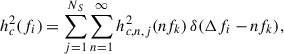 (21)
(21)
where the value of hc, n2 is given by Amaro-Seoane et al. (2010).
4.2. Pulsar timing array: Square Kilometer Array Mid telescope
We used an idealized PTA by employing the SKA (Dewdney et al. 2009), which is planned to be operational in 2027. SKA will be a large radio interferometer telescope whose sensitivity and survey speed will be an order of magnitude greater than any current radio telescope. For this work, we simulate the same array as the one presented in Truant et al. (2025), i.e., a 30 year SKA PTA with 200 pulsars featuring a white noise of σw = 100 ns and an observing cadence of 14 days. Millisecond pulsars are highly stable astrophysical clocks. However, when observed over long timescales, they exhibit intrisic rotational instabilities. In PTAs, these instabilities manifest as a red noise process in the timing residuals, typically at lower frequencies. Specifically, this noise appears as an achromatic red noise process, meaning it is independent of the observed radio frequency. Hence, to ensure a more realistic representation consistent with current observations from PTA datasets, we also included pulsar-intrinsic red noise in the total noise power spectral density in Eq. (18), and we characterized its contribution as a power law (see e.g Lentati et al. 2015):
 (22)
(22)
where Ared corresponds to the amplitude at one year and γred is the spectral index. The red noise properties are chosen to be consistent with those measured in the EPTA DR2Full. To this end, we fit a linear log Ared − γ relation to the measured red noises in Table 4 of EPTA Collaboration and InPTA Collaboration (2023b). Then, we assign Ared and γ parameters according with this relation to 30% of the pulsars in the SKA array, extracting Ared randomly from a uniform log-distribution in the interval −15 < log10(Ared) < − 14, for which the corresponding γ is > 3. In this manner, we mimic the fraction and properties of EPTA DR2Full pulsars in the SKA array with a robust red noise contribution. Note that while the remaining 70% pulsars will likely display some lower level of red noise, this is unlikely to affect the properties of the detected CGWs. In fact, for those pulsars the main stochastic red noise component is going to be the sGWB itself, which is already included in our calculation. We refer to Truant et al. (2025) for the sensitivity curve associated with this PTA experiment. We assume that an MBHB is detected by SKA PTA as a CGW when its S/N ≥ 5.
Finally, the sky position of the 200 pulsars has been set similarly to Truant et al. (2025). In brief, we draw a realistic sky distribution by using the pulsar population synthesis code PsrPopPY6 (Bates et al. 2014). This code generates and evolves realistic pulsar populations drawn from physically motivated models of stellar evolution, calibrated against observational constraints on pulse periods, luminosities, and spatial distributions. The final population of pulsars (105) is selected such that they would be observable (S/N > 9) by a SKA survey with an antenna gain of 140 K/Jy and integration time of 35 minutes. To avoid a particularly (un)fortunate pulsar sky disposition from this distribution, we select a set of 200 pulsars randomly chosen according to a weight given by their radio flux. This procedure is done for each one of the 200 MBHB populations presented in Section 2.5. The sky distribution of one realization of SKA pulsars is presented in the upper panel of Fig. 1. Since PsrPopPy simulates realistic distributions of pulsars generated using theoretical considerations and observational constraints, the bulk of the generated full population of pulsars lies close to the Galactic plane.
5. CGW sky-localization and potential hosts
The success of multimessenger astronomy depends on unequivocally identifying in the sky the AGN or galaxy associated with the detected CGW. This requires having some priors in the source RA and Dec together with its luminosity distance (or its equivalent redshift). In particular, PTA experiments can give constraints in sky localization (θ,ϕ) = (π/2 − Dec,RA) but generally not in luminosity distance. In fact, chirp mass and luminosity distance can only be disentangled by measuring the GW frequency evolution, ḟ, which is typically not possible for the bulk of PTA targets (Sesana & Vecchio 2010). Under these circumstances, it is only possible to constrain the GW amplitude of the source, ζ, i.e., a combination of the chirp mass, ℳz, and the luminosity distance, DL. We acknowledge that ḟ might be detected for some high-frequency, high S/N CGWs, especially for long observation times, such as the 30 years considered here. However, in this work, we make the conservative assumption that ḟ cannot be measured. In the next sections, we describe the selection of the sky-localization area and how we selected the final host candidates to perform multimessenger follow-ups within that sky area.
5.1. Defining the sky localization area
Given the lack of constraints on the luminosity distance, the sky error box associated with the CGW will consist of a region in the (θ, ϕ) plane. To determine the area and shape of this region we follow Goldstein et al. (2019) and make use of a likelihood defined as
![Mathematical equation: $$ \begin{aligned} \mathcal{L} (\theta ,\phi ) \,{=}\, \dfrac{1}{\sqrt{(2\pi )^{^3}\det \Gamma ^{-1}}} \exp {\left[-\dfrac{1}{2} (\boldsymbol{\lambda _i} - \boldsymbol{\lambda _c})^\mathrm{T} \, \Gamma \, (\boldsymbol{\lambda _i} - \boldsymbol{\lambda _c}) \right]}, \end{aligned} $$](/articles/aa/full_html/2026/02/aa54846-25/aa54846-25-eq52.gif) (23)
(23)
where Γ−1 is the 2 × 2 covariance matrix for the θ and ϕ parameters. The vector λi = {θi, ϕi} represents the position of the ith-galaxy in the sky and λc = {θc, ϕc} corresponds to a random point in the sky selected randomly from a 2-dimensional Gaussian probability density function with centers given by the true values of the hosts (θh, ϕh) and variances the ones computed from the Fisher matrix7. Taking into account Eq. (23), the error box associated with a CGW (hereafter Ω90) will be defined as the sky region containing 90% of the likelihood. Similarly, the total number of galaxies or AGNs candidates to be the true hosts (hereafter N100) will be the ones included within Ω90. To guide the reader, in Fig. 4 we present two examples of the sky-localization areas associated with two detected CGWs at different S/N. As expected, the source featuring the larger S/N is better localized.
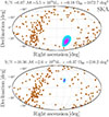 |
Fig. 4. Sky-localization of two different random sources inside our light cones (blue and purple areas). The upper one features a S/N ∼ 6, while the lower one corresponds to S/N ∼ 10. The orange points correspond to the position of the SKA PTA (different from sample to sample as explained in Section 4.2). |
5.2. Reducing the number of candidates within the sky-localization area
The absence of information concerning the luminosity distance of the CGW means that no redshift constraints can be applied to the galaxies within Ω90. This leads to a large number of potential host candidates, even in small areas, which complicates practical multimessenger follow-ups. To lower the value of N100, we follow Goldstein et al. (2019) which showed that the number of potential candidates within Ω90 can be significantly decreased by exploiting the physical dependence of the CGW amplitude with the MBHB chirp mass and distance to the observer, together with empirical MBH mass-host galaxy correlations. Considering this, we assign to the ith-galaxy within Ω90 a probability, 𝒫, of being the true host according to the three-dimensional likelihood function (ℒ(θ, ϕ, lnζ)) and the prior probability (P) which encapsulates the correlation between the galaxy and MBH properties.
Following Section 5.1 and under the assumption of a high S/N, the likelihood marginalized over θ, ϕ, and lnζ (hereafter, ℒ(θ, ϕ, lnζ)) can be written as a 3D multivariate Gaussian centered on the most probable parameter values:
![Mathematical equation: $$ \begin{aligned} \mathcal{L} (\theta ,\phi ,\ln \zeta ) \,{=}\, \dfrac{1}{\sqrt{(2\pi )^{^3}\det \Gamma ^{-1}}} \exp {\left[-\dfrac{1}{2} (\boldsymbol{\lambda _i} - \boldsymbol{\lambda _c})^\mathrm{T} \, \Gamma \, (\boldsymbol{\lambda _i} - \boldsymbol{\lambda _c}) \right]}. \end{aligned} $$](/articles/aa/full_html/2026/02/aa54846-25/aa54846-25-eq53.gif) (24)
(24)
In this case, Γ−1 corresponds to the 3 × 3 covariance matrix for the θ, ϕ, lnζ values8. The vector λc = {θc, ϕc, lnζc} corresponds to a random point in the sky and GW amplitude selected randomly from a 3D Gaussian probability density function with centers given by the true values of the hosts (θh, ϕh, ζh) and its variance being the one computed from the Fisher matrix. For consistency, the values of θc, ϕc were fixed to the ones computed in the Section 5.2. The vector λi = {θi, ϕi, lnζi} represents the sky position and GW amplitude of the possible MBHB placed in the ith-galaxy. The value of ζi was computed according to
![Mathematical equation: $$ \begin{aligned} \zeta _i \,{=}\, \left[\dfrac{G^{5/3}}{c^4 D_{L,i}}\right] \left[\dfrac{(1 \,{+}\, z_i)\,{M}_{\mathrm{{MBH}},i} \,q_i^{3/5} }{(1\,{+}\,q_i)^{6/5}} \right]^{5/3}, \end{aligned} $$](/articles/aa/full_html/2026/02/aa54846-25/aa54846-25-eq54.gif) (25)
(25)
where DL, i is the ith-galaxy luminosity distance assumed to be known once its redshift (zi) is measured, qi is the binary mass ratio selected randomly between [0.01 − 1], and MMBH, i is the total mass of the binary assumed to be placed in the ith-galaxy and drawn from the well-established scaling relation between the MBH and galaxy bulge (MBulge):
 (26)
(26)
Here, α and β set the slope and amplitude of the relation. We relied on the results presented in Chen et al. (2019), which indicated α = 8.40. Concerning the normalization, we followed EPTA Collaboration and InPTA Collaboration (2024) and selected β = 1.01, which led to an agreement with the recent result presented in EPTA Collaboration and InPTA Collaboration (2023a). On top of this, we assumed that the relation presented in Eq. (26) displays an intrinsic scatter, ϵ, set to a conservative number of ϵ = 0.4. We stress that we did not assume any redshift evolution of the scaling relation given that this is still under debate (see Marshall et al. 2020, and references therein).
On the other hand, the prior that we used corresponds to the well-established relation between the MBH mass and the galaxy stellar bulge mass (MBulge):
![Mathematical equation: $$ \begin{aligned}&P({M_{\rm {MBH}} | M_{\rm {Bulge}}}) \,{=}\, \nonumber \\&\dfrac{1}{\sqrt{2\pi \epsilon ^2}} \exp \left\{ - \dfrac{ \biggl [ \log _{10} \dfrac{M_{\rm {MBH}}}{\mathrm{{M}_\odot }} - \biggl ( \alpha + \beta \log _{10} \left( \dfrac{M_{\rm {Bulge}}}{10^{11}\, \mathrm {M}_\odot } \right) \biggr )^2 \Biggr ] }{2 \epsilon ^2} \right\} , \end{aligned} $$](/articles/aa/full_html/2026/02/aa54846-25/aa54846-25-eq56.gif) (27)
(27)
where ϵ corresponds to the intrinsic scatter of the relation. For simplicity, we assumed that the galaxy bulge mass is always know, and we set the ϵ value to the conservative value of 0.4.
By combining Eq. (24) and Eq. (27), the probability P of the ith-galaxy to be the true host can be written as
 (28)
(28)
where q is assumed to have flat prior between the reasonable range [qmin, qmax] = [0.01 − 1] and [MMBH, min, MMBH, max] = [Eq. (26) − 3ϵ, Eq. (26) + 3ϵ]. We refer to Goldstein et al. (2019) for further details about the methodology.
After quantifying the values of P for all galaxies within Ω90, we normalize the total probability across the sky-localization area and rank the galaxies from the most to the least probable. We then calculate the cumulative probability for the entire galaxy sample and select only those objects that contribute to 90% of the total probability. These selected galaxies will be tagged as N90 and will be the only ones used in our search for the true CGW host. By construction, there is a 90% probability that the true host lies within the N90 sample.
6. Results
We present our main results in this section. We investigate the AGN counterparts of the detected MBHBs and the properties of the galaxies in which they are hosted. We then discuss challenges and strategies for unequivocally identifying the MBHB host within its sky-localization error box.
6.1. Resolvable MBHBs and their properties
In Fig. 5 we show the distribution of the number of resolvable sources (Nres) in our light cones. The distribution is broad, with a plateau extending from 15 to 40 and a median value ∼33.
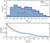 |
Fig. 5. Upper panel: Distribution of the number of MBHBs resolved by the 30 year SKA (Nres) in each light cone generated by L-Galaxies. Lower panel: Cumulative distribution function of the signal-to-noise ratio for the resolved MBHBs. |
In the same plot, we have divided the distribution between the Fiducial and Boosted models, showing that the cases with large Nres correspond to the latter models where the sGWB is larger than the average one of our populations (see Fig. 2). These results agree with the recent work of Truant et al. (2025) which, using populations of MBHBs in agreement with recent PTA results, showed that a 30 year SKA PTA would be able to resolve on average ≈30 CGWs, with a mild dependence on the typical eccentricity of the MBHB population. The lower panel of Fig. 5 displays the cumulative distribution function of the S/N of the resolved sources: 90% of the CGW feature S/N ≲ 15, with a long tail extending to S/N ≈ 100. Considering that, on average the array can detect ≈33 CGWs, the typical highest S/N in a single universe realization is around 20–25.
In Fig. 6 we present the properties of the detected MBHBs. As we can see, the detected sources can be found up to z ∼ 2 but the bulk of the CGWs are sourced by MBHBs at z < 0.5. The minimum chirp is ℳ ∼ 108.5 M⊙, but typical values are in the range 109 M⊙ − 109.5 M⊙. The mass ratios are distributed in the range 0.1 < q < 1, with a peak toward equal masses.
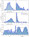 |
Fig. 6. Properties of the detectable sources by 30 year SKA: Chirp mass distribution (ℳ, upper left panel), redshift (z, upper right panel), twice the observed Keplerian frequency (f2, center left panel), eccentricity (e, center right panel), mass ration (q, lower left panel), and inclination angle (i, lower right panel) of the detected MBHBs. The term NBin represents the number of objects in a given bin of the histogram, while Ntot is the total number of objects analyzed. For reference, we present with black lines the distribution of eccentricity and inclination angle for all the MBHBs presented inside the light cone. |
Eccentricities tend to be small, with a clear predominance of values e < 0.2, although a long tail of eccentric binaries extends up to e ≳ 0.8 The fundamental GW frequency (i.e., twice the Keplerian frequency, f2) of the MBHBs peaks at 10−8 Hz and declines rapidly toward larger values. Interestingly, there are a few cases where the frequency is smaller than the one associated 1/Tobs. As described in Truant et al. (2025), these sources are eccentric MBHBs that can enter inside the PTA band thanks to the power emission along many different harmonics. Finally, the inclination distribution features a bimodality, having a preference for face-on/face-off binaries. This can be simply explained by the angular pattern emission of GWs, which are stronger along the binary orbital angular momentum axis. These properties along with previous results indicate that future detection of nanohertz MBHBs will unveil the most massive population of MBHBs in the local Universe (see similar results in, e.g., Rosado et al. 2015; Kelley et al. 2018; Cella et al. 2025).
Once the properties of the detected MBHBs have been characterized, it is interesting to explore their emission properties. The upper panel of Fig. 7 presents the cumulative distribution function of the associated AGN magnitudes in the optical u, g, r, i, z filters. As we can see, less than 20% of them feature an optical emission with magnitude mag < 30 independently of the filter. This implies that a large fraction of our detected MBHBs will be essentially inactive, hindering the identification of the CGW-EM counterpart based on AGN selection. This fraction decreases down to ≈10% when we request that the AGN counterpart associated with the MBHB is optically detectable by LSST. In the lower panel of Fig. 7 we present the cumulative distribution function of the X-ray counterpart associated with the MBHB9. As shown, only 50% of the sources display hard 2−10 keV and soft 0.5−2 keV X-ray fluxes > 10−19 erg s−1 cm−2. This value drops down to 5% when fluxes > 10−14 erg s−1 cm−2 are imposed. The X-ray emission is compared with the detection limit of eRosita (Merloni et al. 2012). As we can see, only ∼3% of the sources will be detected in the soft X-rays and none in the hard X-rays by eRosita. Considering next-generation X-ray observatories such as Athena (Piro et al. 2023) yields more promising results. With flux limits of 2 × 10⁻¹⁷ erg s−1 cm−2 and 10−16 erg s−1 cm−2 in the soft and hard X-ray respectively, up to 20% of the systems might be within reach for Athena. However, as we show below, the tipical source localization in the sky is poor, and tailing the location error region with long Athena exposures might be unfeasible. As discussed in Section 3, we stress that the X-ray results should be considered upper limits since attenuation due to neutral gas has not been included.
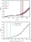 |
Fig. 7. Upper panel: Cumulative distribution function of the AGN magnitude associated with the MBHB sourcing the CGWs. Each color corresponds to a different LSST filter: u, g, r, i, z. Dashed vertical lines represent the limiting magnitudes of the LSST in each filter. Lower panel: Cumulative distribution function of the X-ray flux in the soft (0.5–2 KeV, green) and hard X-ray (2–10 KeV, purple) bands. Dashed vertical lines highlight the detection limit of eRosita. |
Based on the results presented above and considering an average number of 33 resolved CGWs, three-four of them might be associated with weak optical AGNs and only one might be associated with soft-X AGN activity within the eROSITA sensitivity limits. This suggests that multimessenger studies with PTA should also consider the search for the galaxy host rather than focusing exclusively on AGNs.
6.2. Host galaxy properties
In Fig. 8 we present the properties of the galaxies hosting the detected MBHBs. As shown, these systems are typically harbored in massive M★ > 1011 M⊙ elliptical (bulge-to-total ratio B/T > 0.9) galaxies, although there are cases where the galaxy can be disk-dominated (B/T < 0.4). Fig. 8 also depicts the specific star formation rate (sSFR) of these galaxies. The values are typical for massive galaxies, with most hosts lying in the range 10−12 yr−1 < sSRF < 10−10 yr−1. However, there is a long tail (> 50%) of passive hosts extending down to sSRF ∼ 10−15 yr−1.
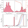 |
Fig. 8. Properties of the galaxies hosting the MBHBs sourcing the CGWs detected by 30 year SKA: Galaxy stellar mass (M*, upper left), sSFR (upper right), bulge-to-total ratio (B/T, lower left), and stellar magnitude in the (u, g, r, i, z) set of filters (lower right). In the panel with the sSFR, the vertical line highlights the 10−11 yr−1 value. On the other hand, the blue line corresponds to the cumulative distribution. Finally, the vertical lines correspond to the magnitude limits of LSST in the u, g, r, i, z filters. |
The lower panel of Fig. 8 presents the cumulative distribution function of the galaxy magnitude in the (u, g, r, i, z) filter set. As we can see, the detection of galaxies in the bluer filters (u, g) is disfavored with respect to the redder ones (r, i, z) given that their distributions are shifted toward larger magnitudes (i.e., lower fluxes). For instance, ∼90% of the sources in the r filter feature < 23 mag while only ∼50% feature the same limit in the u filter band. These results, together with the sSFR distributions, imply that the hosts of the detected MBHBs will be placed in red galaxies (see similar results in Cella et al. 2025). Finally, when comparing the magnitude distributions with the LSST expected magnitude limits, we can see that the vast majority of the objects will be detected. This value reaches ≈100% for (g, r, i, z) filters and ≈85% for the u filter.
6.3. Host identification
In this section, we explore the feasibility of unequivocally identifying the galaxy host of the MBHB sourcing the CGW detected by the SKA PTA. To this end, we explored the typical sky localization area, the number of galaxies within it, and different selection techniques to reduce the number of host candidates. We stress that we only considered galaxies that are observable in the r-band, which is the deepest of the LSST filters10. We refer to Appendix A for the magnitude distribution of the host candidates.
6.3.1. Potential hosts: Number and properties
Figure 9 presents the distribution of Ω90 for all SKA PTA resolvable CGW sources. The distribution peaks at ≈ 300 deg2 indicating that the search of the galaxy hosting the MBHB can be strongly disfavored. Despite that, ∼35% of the detected sources feature Ω90 < 100 deg2. From hereafter, we examine the feasibility of unequivocally identifying the CGW hosts for those systems with Ω90 < 100 deg2. To guide the reader, the left and right panels of Fig. 10 depict two examples of galaxy distributions within the sky-localization regions associated to a detected CGW with Ω90 < 100 deg2. As shown, the lack of redshift constrains results in the true host being buried among hundreds of thousands of galaxies observable by LSST. However, as demonstrated in the middle panel of Fig. 10, by applying the methodology described in Section 5 we can significantly reduce the number of potential candidates.
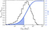 |
Fig. 9. Histogram and cumulative density function (in blue) of Ω90 of the resolved sources. The light blue area represents the CGW with an Ω90 < 100 deg2 for which we consider for a possible EM follow-up. |
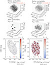 |
Fig. 10. Distribution in the (RA, Dec, z) space of the galaxies with M∗ > 1010.3 M⊙ and the r-band < 27.5 mag placed within the sky-localization area constrained by SKA PTA. Top panel: Distribution of the galaxies when no probability selection is performed. N100 indicates the total number of these galaxies. Middle panel: Same as top panel but when presenting only the galaxies that contribute to the 90% probability of being the true host (see Section 5). The size of the circle is proportional to the probability. Lower panel: Right ascension and declination plane. The gray (colored) points correspond to all the galaxies in the N100 (N90) sample. The color encodes the photometric color i − z. |
To quantify the trend presented above, in Fig. 11 we present the number of candidates within the sky-localization area depending on the source S/N (see similar results in Tanaka et al. 2012). Without any selection procedure, the total number of candidates (N100) varies between 3 × 10⁴ − 2 × 10⁵, being the CGWs with larger S/N the ones featuring the lowest values. These large numbers would hinder a viable search for the true host. However, when we select only galaxies contributing 90% (N90) and 50% (N50) of the whole probability, the number of candidates drops by 2−5 dex, depending on the S/N. Despite this improvement, CGWs detected at S/N ≲ 25 still have a large number of potential hosts (> 100). Conversely, the origin of the rarer CGWs detected with S/N > 25 can be traced to < 100 potential candidates, making them promising targets for multimessenger studies.
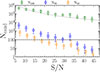 |
Fig. 11. Number of candidates (Ncand) within the sky-localization area depending on the S/N of the detected CGW source. Green circles correspond to the total number of galaxies with M∗ > 1010.3 M⊙ within the detection area (N100). Blue and orange circles represent the same thing, but only including the galaxies contributing 90% and 50% of the total probability of being the true host. To improve the plot clarity, orange points have been shifted by a factor of 0.5. The gray line corresponds to the expected 1/(S/N)2 relation. |
6.3.2. Strategies for identifying hosts of CGWs with S/N< 25: Galaxy color cuts
As shown in the previous section, CGWs detected at S/N > 25 have N90 ≲ 100, making them the perfect targets for multimessenger follow-ups. However, these cases are rare, accounting for less than 5% of the future detections (i.e., ≈1 CGW in a 30 yr SKA PTA, see Fig. 5). On the other hand, CGWs with S/N < 25 represent the most common scenarios, but they typically features 102 < N90 < 104. Therefore, it is crucial to investigate whether candidates linked to CGWs with S/N < 25 show any differences in the optical properties compared to the true host, that can be easily identified by LSST11.
In Fig. 12 we present the distribution of the optical color of the candidate galaxies (N90) and true CGW hosts. Specifically, we have explored u − g, g − r, r − i and i − z12. For instance, while the former color encodes the current star formation activity of the galaxy, the latter traces its past star formation history (see, e.g., Strateva et al. 2001). As presented in the figure, the distributions of the two samples overlap in all the presented colors and feature two predominant peaks at comparable values. For example, in the case of u − g, the true hosts exhibit a primary peak at 0.1 and a secondary one at 2.5. Host candidates also display a similar bi-modality, but their primary peak occurs at u − g = 2.5. This behavior stems from the fact that galaxies composing the two samples are formed by star-forming (bluer colors) and passive (redder colors) systems. However, the relative abundance of these two classes of galaxies varies between the CGW hosts and N90. While the predominant peak in the colors of the CGW hosts rises due to the predominance of passive galaxies, the peak in the N90 sample is made of star-forming galaxies. We observed a similar trend in the r − i and i − z colors, although the two peaks convey slightly different information. The peaks at lower values correspond to galaxies that have undergone a recent star formation event, which is now nearly complete or already finished, resulting in a mix of old and young stellar populations. For instance, in the case of CGW hosts, this last star formation process is likely associated with the galaxy merger that led to the formation of the MBHB. In contrast, the peaks at higher values represent galaxies with very evolved and old stellar populations that have not experienced any significant star formation activity in the past gigayear.
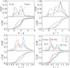 |
Fig. 12. Upper panels: Probability distribution function of the u − g, g − r, r − i, and i − z colors for the galaxies within the sky-localization area (N100, green), the galaxies within the sky-localization area contributing to the 90% probability of being the true host (N90, blue), and the true host (Host, red). Lower panel: Cumulative distribution function of the u − g, g − r, r − i, and i − z colors for N100, N90, and true host. In all the plots, the distributions correspond to the galaxies associated with CGWs whose S/N < 25. |
To determine if a simple color cut can reduce a significant fraction of the N90 galaxies, in the lower panels of Fig. 12 we present the cumulative distribution function (CDF). As shown, the g − r color is the one that provides the worst candidate reduction, since the CDF of candidates and true hosts are very similar. In contrast, the i − z and r − i colors are the most effective ones at distinguishing between candidates and true hosts. For instance, in the case of i − z (r − i), we can reduce the number of sources by focusing on the 65% of candidates that have colors ≲0.80 (≲1.15) which are compatible with those of the CGW hosts. In Table. 1 we summarize the color cut required to minimize the risk of excluding the true host while reducing the number of potential candidates. As depicted in the table, the most promising scenario only envisions the reduction of ∼37% of the sources, which does not add decisive information for efficient multimessenger follow-up of low S/N CGWs (see Fig. 11). Due to the absence of a single color cut that could effectively narrow down the candidate pool, in Fig. 13 we investigate whether the potential candidates and true host galaxies occupy distinct regions in color-color space. As shown, no significant differences are seen in any of the color diagrams explored.
Fraction of N90 galaxies removed after applying different optical color cuts with LSST filters.
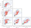 |
Fig. 13. Color-color diagrams for the galaxies hosting the CGW (Hosts, red circles) and the galaxies inside the sky-localization area contributing to 90% probability (N90, blue contours). In all the plots, the distributions correspond to the galaxies associated with CGWs with S/N < 25. Green circles represent the region where AGNs are expected to be placed in the color-color diagram. |
Considering the results presented above, the absence of a definitive method to significantly narrow down the candidate pool underlines the complexities involved in identifying suitable PTA CGW sources for multimessenger follow-up observations.
7. Conclusions
In this paper, we have investigated the feasibility of performing multimessenger astronomy with continuous CGWs detected by an idealized 30 year SKA PTA. To this end, we employed the L-Galaxies SAM applied to the Millennium simulation. Specifically, we generated 200 different all-sky light cones that include galaxies, MHBs, and MBHBs whose emission has been modeled consistently based on their star formation histories and gas accretion physics. By applying the detection methodology presented in Truant et al. (2025) in our simulated universes, we found the following:
-
The SKA PTA is expected to detect an average of ∼33 CGWs. The majority of these detections (> 90%) have an S/N lower than 15.
-
The detected CGW signals come from MBHBs placed at a low-z (z < 0.5) with masses of ∼ 3 × 10⁹ M⊙, mass ratios > 0.1, and eccentricities ≲0.2.
-
Only 10% of the detected CGWs are related to an AGN with an optical magnitude of ≲ 27 mag, i.e., the typical detection limit of the deep-observing mode of LSST. Furthermore, only about 3% of the CGWs reach the detection limit of the e-Rosita X-ray telescope.
-
Detected CGWs are hosted in massive (M★ > 1011 M⊙) elliptical (B/T > 0.9) galaxies with a typical sSFR easily detectable by LSST in the redder bands (< 23 mag).
In light of these results, our study suggests that the unequivocal EM detection of PTA CGW counterparts should prioritize the search for galaxies over AGNs. With this in mind, we explored the potential of conducting multimessenger astronomy using the legacy data of LSST, which will allow us to create complete sky galaxy catalogs over about half of the sky. Our findings have shown that the typical sky-localization of our CGW sources is ∼ 300 deg2, with about 35% of them associated with areas < 100 deg2. Given the large sky-localization regions, we have only investigated the feasibility of unequivocally identifying the CGW hosts in the cases where the restricted area is less than 100 deg2. The results can be summarized as follows:
-
The total number of candidates detectable by LSST (N100) varies between 3 × 10⁴ − 2 × 10⁵. As expected, the CGWs with larger S/N ratios are the ones that feature the lowest N100 values because of their better sky-localization areas.
-
The number of potential candidates within the sky-localization area can be significantly reduced by using the methodology outlined in Goldstein et al. (2019). This approach assigns a probability of being the true hosts by examining the physical relationship between the CGW amplitude and the MBHB chirp mass, alongside empirical correlations between MBH mass and its host galaxy. By selecting only those candidates that contribute to the 90% of the total probability (N90), we find that for systems with S/N < 25, the values of N90 falls between 103 − 100. For sources with an even higher S/N, N90 decreases to a range between 100 − 5, making them the perfect sources for multimessenger follow-ups.
-
In cases where CGWs are detected with a low S/N (< 25), applying certain optical color cuts can help reduce the number of N90. Specifically, the i − z color is the most effective for this purpose, as it distinguishes between galaxies with an old or mixed stellar population. For example, by selecting only galaxies with colors of i − z < 0.80, we can eliminate up to 37% of galaxies within the N90 while having only a 20% chance of mistakenly discarding the true host. Similar results have been found for the r − i color. Despite this improvement, the number of candidates is still large. Color-color diagrams can also help in reducing N90, but no strong improvement with respect to a single color cut has been noticed.
-
In cases where CGWs are detected with a large S/N (> 25), optical color cuts are more efficient in reducing the number of N90 candidates. In these cases, a cut in i − z < 0.33 can eliminate up to 70% of galaxies within the N90 with a 20% chance of mistakenly discarding the true host. This means that in these cases, the number of candidates can typically be reduced to less than 50.
We stress that these findings are based on a few conservative assumptions. One important caveat is that we assumed that PTAs cannot measure the frequency evolution (ḟ) of the CGW. Although this is a realistic assumption in most cases, it might be possible for an SKA array to measure ḟ for some high S/N, high-frequency CGWs. This would allow a constraint to be placed on the source luminosity distance, possibly substantially narrowing down the number of candidate host galaxies within the (now 3D) error volume. Furthermore, in our Fisher analysis we ignored the CGW pulsar terms, which might significantly improve source sky localization and distance measurement. It should be noted, however, that identification of individual pulsar terms, especially in the presence of multiple overlapping CGWs in the data, might be extremely challenging, and moreover, it has not been demonstrated.
In summary, our investigation indicates that CGWs detected with a high S/N will serve as ideal sources for conducting multimessenger studies with optical follow-ups. However, these studies will be more challenging for MBHBs detected with a low S/N, as there is no definitive methodology to significantly reduce the pool of candidates within their sky-localization areas. Since CGW detections will be dominated by low S/N systems, multimessenger astronomy involving PTA sources is anticipated to be challenging.
Acknowledgments
We thank the B-Massive group at Milano-Bicocca University for useful discussions and comments. R.T., D.I.V., A.S. and G.M.S acknowledge the financial support provided under the European Union’s H2020 ERC Consolidator Grant B Massive (Grant Agreement: 818691) and Advanced Grant PINGU (Grant Agreement: 101142097). M.B. acknowledges support provided by MUR under grant “PNRR – Missione 4 Istruzione e Ricerca - Componente 2 Dalla Ricerca all’Impresa – Investimento 1.2 Finanziamento di progetti presentati da giovani ricercatori ID:SOE_0163” and by University of Milano-Bicocca under grant “2022-NAZ-0482/B”. S.B. acknowledges support from the Spanish Ministerio de Ciencia e Innovación through project PID2021-124243NB-C21.
References
- Agazie, G., Anumarlapudi, A., Archibald, A. M., et al. 2023, ApJ, 951, L8 [NASA ADS] [CrossRef] [Google Scholar]
- Amaro-Seoane, P., Sesana, A., Hoffman, L., et al. 2010, MNRAS, 402, 2308 [NASA ADS] [CrossRef] [Google Scholar]
- Angulo, R. E., & White, S. D. M. 2010, MNRAS, 405, 143 [NASA ADS] [Google Scholar]
- Arzoumanian, Z., Brazier, A., Burke-Spolaor, S., et al. 2015, ApJ, 810, 150 [NASA ADS] [CrossRef] [Google Scholar]
- Arzoumanian, Z., Baker, P. T., Brazier, A., et al. 2021, ApJ, 914, 121 [Google Scholar]
- Ayromlou, M., Nelson, D., Yates, R. M., et al. 2021, MNRAS, 502, 1051 [NASA ADS] [CrossRef] [Google Scholar]
- Babak, S., & Sesana, A. 2012, Phys. Rev. D, 85, 044034 [NASA ADS] [CrossRef] [Google Scholar]
- Bates, S. D., Lorimer, D. R., Rane, A., & Swiggum, J. 2014, MNRAS, 439, 2893 [NASA ADS] [CrossRef] [Google Scholar]
- Begelman, M. C., Blandford, R. D., & Rees, M. J. 1980, Nature, 287, 307 [Google Scholar]
- Binney, J., & Tremaine, S. 2008, Galactic Dynamics: Second Edition (Princeton, NJ USA: Princeton University Press) [Google Scholar]
- Bonetti, M., Haardt, F., Sesana, A., & Barausse, E. 2018, MNRAS, 477, 3910 [Google Scholar]
- Bonetti, M., Sesana, A., Haardt, F., Barausse, E., & Colpi, M. 2019, MNRAS, 486, 4044 [NASA ADS] [CrossRef] [Google Scholar]
- Bonetti, M., Rasskazov, A., Sesana, A., et al. 2020, MNRAS, 493, L114 [Google Scholar]
- Bonoli, S., Marulli, F., Springel, V., et al. 2009, MNRAS, 396, 423 [NASA ADS] [CrossRef] [Google Scholar]
- Bortolas, E., Capelo, P. R., Zana, T., et al. 2020, MNRAS, 498, 3601 [Google Scholar]
- Bortolas, E., Bonetti, M., Dotti, M., et al. 2022, MNRAS, 512, 3365 [NASA ADS] [CrossRef] [Google Scholar]
- Burke-Spolaor, S. 2013, Class. Quant. Grav., 30, 224013 [Google Scholar]
- Cella, K., Taylor, S. R., & Zoltan Kelley, L. 2025, Class. Quant. Grav., 42, 025021 [Google Scholar]
- Charisi, M., Bartos, I., Haiman, Z., et al. 2016, MNRAS, 463, 2145 [Google Scholar]
- Charisi, M., Haiman, Z., Schiminovich, D., & D’Orazio, D. J. 2018, MNRAS, 476, 4617 [Google Scholar]
- Chen, S., Sesana, A., & Conselice, C. J. 2019, MNRAS, 488, 401 [NASA ADS] [CrossRef] [Google Scholar]
- Cocchiararo, F., Franchini, A., Lupi, A., & Sesana, A. 2024, A&A, 691, A250 [NASA ADS] [CrossRef] [EDP Sciences] [Google Scholar]
- Croton, D. J. 2006, MNRAS, 369, 1808 [NASA ADS] [CrossRef] [Google Scholar]
- Croton, D. J., Springel, V., White, S. D. M., et al. 2006, MNRAS, 365, 11 [Google Scholar]
- Cuadra, J., Armitage, P. J., Alexander, R. D., & Begelman, M. C. 2009, MNRAS, 393, 1423 [Google Scholar]
- Desvignes, G., Caballero, R. N., Lentati, L., et al. 2016, MNRAS, 458, 3341 [Google Scholar]
- Dewdney, P. E., Hall, P. J., Schilizzi, R. T., & Lazio, T. J. L. W. 2009, IEEE Proc., 97, 1482 [Google Scholar]
- Dotti, M., Colpi, M., Haardt, F., & Mayer, L. 2007, MNRAS, 379, 956 [NASA ADS] [CrossRef] [Google Scholar]
- Dotti, M., Merloni, A., & Montuori, C. 2015, MNRAS, 448, 3603 [NASA ADS] [CrossRef] [Google Scholar]
- Duffell, P. C., D’Orazio, D., Derdzinski, A., et al. 2020, ApJ, 901, 25 [NASA ADS] [CrossRef] [Google Scholar]
- EPTA Collaboration and InPTA Collaboration (Antoniadis, J., et al.) 2023a, A&A, 678, A50 [CrossRef] [EDP Sciences] [Google Scholar]
- EPTA Collaboration and InPTA Collaboration (Antoniadis, J., et al.) 2023b, A&A, 678, A49 [Google Scholar]
- EPTA Collaboration and InPTA Collaboration (Antoniadis, J., et al.) 2024, A&A, 685, A94 [NASA ADS] [CrossRef] [EDP Sciences] [Google Scholar]
- Escala, A., Larson, R. B., Coppi, P. S., & Mardones, D. 2004, ApJ, 607, 765 [NASA ADS] [CrossRef] [Google Scholar]
- Falxa, M., Babak, S., Baker, P. T., et al. 2023, MNRAS, 521, 5077 [NASA ADS] [CrossRef] [Google Scholar]
- Fiacconi, D., Mayer, L., Roškar, R., & Colpi, M. 2013, ApJ, 777, L14 [NASA ADS] [CrossRef] [Google Scholar]
- Fontecilla, C., Chen, X., & Cuadra, J. 2017, MNRAS, 468, L50 [Google Scholar]
- Foster, R. S., & Backer, D. C. 1990, ApJ, 361, 300 [NASA ADS] [CrossRef] [Google Scholar]
- Franchini, A., Sesana, A., & Dotti, M. 2021, MNRAS, 507, 1458 [NASA ADS] [Google Scholar]
- Franchini, A., Lupi, A., & Sesana, A. 2022, ApJ, 929, L13 [NASA ADS] [CrossRef] [Google Scholar]
- Franchini, A., Lupi, A., Sesana, A., & Haiman, Z. 2023, MNRAS, 522, 1569 [NASA ADS] [CrossRef] [Google Scholar]
- Gardiner, E. C., Kelley, L. Z., Lemke, A. M., & Mitridate, A. 2023, arXiv e-prints [arXiv:2309.07227] [Google Scholar]
- Goldstein, J. M., Sesana, A., Holgado, A. M., & Veitch, J. 2019, MNRAS, 485, 248 [NASA ADS] [CrossRef] [Google Scholar]
- Guo, Q., White, S., Boylan-Kolchin, M., et al. 2011, MNRAS, 413, 101 [Google Scholar]
- Haiman, Z., Kocsis, B., & Menou, K. 2009, ApJ, 700, 1952 [CrossRef] [Google Scholar]
- Henriques, B. M. B., White, S. D. M., Thomas, P. A., et al. 2015, MNRAS, 451, 2663 [Google Scholar]
- Henriques, B. M. B., Yates, R. M., Fu, J., et al. 2020, MNRAS, 491, 5795 [NASA ADS] [CrossRef] [Google Scholar]
- Hopkins, P. F., & Quataert, E. 2010, MNRAS, 407, 1529 [Google Scholar]
- Husa, S. 2009, Gen. Rel. Grav., 41, 1667 [Google Scholar]
- Ivanov, P. B., Papaloizou, J. C. B., & Polnarev, A. G. 1999, MNRAS, 307, 79 [Google Scholar]
- Ivezić, Ž., Kahn, S. M., Tyson, J. A., et al. 2019, ApJ, 873, 111 [Google Scholar]
- Izquierdo-Villalba, D., Angulo, R. E., Orsi, A., et al. 2019a, A&A, 631, A82 [NASA ADS] [CrossRef] [EDP Sciences] [Google Scholar]
- Izquierdo-Villalba, D., Bonoli, S., Spinoso, D., et al. 2019b, MNRAS, 488, 609 [NASA ADS] [CrossRef] [Google Scholar]
- Izquierdo-Villalba, D., Bonoli, S., Dotti, M., et al. 2020, MNRAS, 495, 4681 [NASA ADS] [CrossRef] [Google Scholar]
- Izquierdo-Villalba, D., Sesana, A., Bonoli, S., & Colpi, M. 2022, MNRAS, 509, 3488 [Google Scholar]
- Izquierdo-Villalba, D., Sesana, A., Colpi, M., et al. 2024, A&A, 686, A183 [NASA ADS] [CrossRef] [EDP Sciences] [Google Scholar]
- Kelley, L. Z., Blecha, L., Hernquist, L., Sesana, A., & Taylor, S. R. 2018, MNRAS, 477, 964 [Google Scholar]
- Kelley, L. Z., Haiman, Z., Sesana, A., & Hernquist, L. 2019, MNRAS, 485, 1579 [NASA ADS] [CrossRef] [Google Scholar]
- Kramer, M., & Champion, D. J. 2013, Class. Quant. Grav., 30, 224009 [NASA ADS] [CrossRef] [Google Scholar]
- Lee, K. J. 2016, in Frontiers in Radio Astronomy and FAST Early Sciences Symposium 2015, eds. L. Qain, & D. Li, ASP Conf. Ser., 502, 19 [Google Scholar]
- Lentati, L., Taylor, S. R., Mingarelli, C. M. F., et al. 2015, MNRAS, 453, 2576 [Google Scholar]
- Li, K., Bogdanović, T., Ballantyne, D. R., & Bonetti, M. 2022, ApJ, 933, 104 [NASA ADS] [CrossRef] [Google Scholar]
- Lodato, G., Nayakshin, S., King, A. R., & Pringle, J. E. 2009, MNRAS, 398, 1392 [NASA ADS] [CrossRef] [Google Scholar]
- LSST Science Collaboration (Abell, P. A., et al.) 2009, arXiv e-prints [arXiv:0912.0201] [Google Scholar]
- Mahadevan, R. 1997, ApJ, 477, 585 [NASA ADS] [CrossRef] [Google Scholar]
- Manchester, R. N., Hobbs, G., Bailes, M., et al. 2013, PASA, 30, e017 [NASA ADS] [CrossRef] [Google Scholar]
- Marshall, M. A., Mutch, S. J., Qin, Y., Poole, G. B., & Wyithe, J. S. B. 2020, MNRAS, 494, 2747 [NASA ADS] [CrossRef] [Google Scholar]
- Mayer, L., Kazantzidis, S., Madau, P., et al. 2007, Science, 316, 1874 [NASA ADS] [CrossRef] [Google Scholar]
- McLaughlin, M. A. 2013, Class. Quant. Grav., 30, 224008 [NASA ADS] [CrossRef] [Google Scholar]
- Merloni, A., Predehl, P., Becker, W., et al. 2012, arXiv e-prints [arXiv:1209.3114] [Google Scholar]
- Miles, M. T., Shannon, R. M., Bailes, M., et al. 2023, MNRAS, 519, 3976 [NASA ADS] [CrossRef] [Google Scholar]
- Miles, M. T., Shannon, R. M., Reardon, D. J., et al. 2025, MNRAS, 536, 1489 [Google Scholar]
- Milosavljević, M., & Merritt, D. 2001, ApJ, 563, 34 [Google Scholar]
- Mingarelli, C. M. F., Lazio, T. J. W., Sesana, A., et al. 2017, Nat. Astron., 1, 886 [Google Scholar]
- Peters, P. C., & Mathews, J. 1963, Phys. Rev., 131, 435 [Google Scholar]
- Petrov, P., Taylor, S. R., Charisi, M., & Ma, C.-P. 2024, ApJ, 976, 129 [Google Scholar]
- Piro, L., Colpi, M., Aird, J., et al. 2023, MNRAS, 521, 2577 [NASA ADS] [CrossRef] [Google Scholar]
- Planck Collaboration XVI. 2014, A&A, 571, A16 [NASA ADS] [CrossRef] [EDP Sciences] [Google Scholar]
- Quinlan, G. D., & Hernquist, L. 1997, New Astron., 2, 533 [NASA ADS] [CrossRef] [Google Scholar]
- Ragusa, E., Lodato, G., & Price, D. J. 2016, MNRAS, 460, 1243 [CrossRef] [Google Scholar]
- Ravi, V., Wyithe, J. S. B., Shannon, R. M., & Hobbs, G. 2015, MNRAS, 447, 2772 [NASA ADS] [CrossRef] [Google Scholar]
- Reardon, D. J., Hobbs, G., Coles, W., et al. 2016, MNRAS, 455, 1751 [NASA ADS] [CrossRef] [Google Scholar]
- Reardon, D. J., Zic, A., Shannon, R. M., et al. 2023, ApJ, 951, L6 [NASA ADS] [CrossRef] [Google Scholar]
- Regan, J. A., Downes, T. P., Volonteri, M., et al. 2019, MNRAS, 486, 3892 [CrossRef] [Google Scholar]
- Rosado, P. A., & Sesana, A. 2014, MNRAS, 439, 3986 [NASA ADS] [CrossRef] [Google Scholar]
- Rosado, P. A., Sesana, A., & Gair, J. 2015, MNRAS, 451, 2417 [NASA ADS] [CrossRef] [Google Scholar]
- Sersic, J. L. 1968, Atlas de Galaxias Australes (Cordoba, Argentina: Observatorio Astronomico) [Google Scholar]
- Sesana, A., & Khan, F. M. 2015, MNRAS, 454, L66 [Google Scholar]
- Sesana, A., & Vecchio, A. 2010, Phys. Rev. D, 81, 104008 [NASA ADS] [CrossRef] [Google Scholar]
- Sesana, A., Haardt, F., & Madau, P. 2006, ApJ, 651, 392 [Google Scholar]
- Sesana, A., Vecchio, A., & Volonteri, M. 2009, MNRAS, 394, 2255 [NASA ADS] [CrossRef] [Google Scholar]
- Shakura, N. I., & Sunyaev, R. A. 1973, A&A, 24, 337 [NASA ADS] [Google Scholar]
- Shen, X., Hopkins, P. F., Faucher-Giguère, C.-A., et al. 2020, MNRAS, 495, 3252 [Google Scholar]
- Simon, J., Polin, A., Lommen, A., et al. 2014, ApJ, 784, 60 [Google Scholar]
- Spinoso, D., Bonoli, S., Valiante, R., Schneider, R., & Izquierdo-Villalba, D. 2023, MNRAS, 518, 4672 [Google Scholar]
- Springel, V., White, S. D. M., Tormen, G., & Kauffmann, G. 2001, MNRAS, 328, 726 [Google Scholar]
- Springel, V., White, S. D. M., Jenkins, A., et al. 2005, Nature, 435, 629 [Google Scholar]
- Strateva, I., Ivezić, Ž., Knapp, G. R., et al. 2001, AJ, 122, 1861 [CrossRef] [Google Scholar]
- Susobhanan, A., Maan, Y., Joshi, B. C., et al. 2021, PASA, 38, e017 [Google Scholar]
- Tanaka, T., Menou, K., & Haiman, Z. 2012, MNRAS, 420, 705 [Google Scholar]
- Truant, R. J., Izquierdo-Villalba, D., Sesana, A., Shaifullah, G. M., & Bonetti, M. 2025, A&A, 694, A282 [NASA ADS] [CrossRef] [EDP Sciences] [Google Scholar]
- Vasiliev, E., Antonini, F., & Merritt, D. 2014, ApJ, 785, 163 [Google Scholar]
- White, S. D. M., & Frenk, C. S. 1991, ApJ, 379, 52 [Google Scholar]
- Xu, H., Chen, S., Guo, Y., et al. 2023, Res. Astron. Astrophys., 23, 075024 [CrossRef] [Google Scholar]
- Yates, R. M., Henriques, B. M. B., Fu, J., et al. 2021, MNRAS, 503, 4474 [NASA ADS] [CrossRef] [Google Scholar]
- Yu, Q. 2002, MNRAS, 331, 935 [Google Scholar]
These masses are covered by the merger trees extracted from the Millennium-II, TNG-DARK00 and TNG-DARK50 simulations.
We stress that in this work we do not consider the y filter since we only used the filters in common with the Sloan Digital Sky Survey.
Notice that  , being z the redshift of the source and Lν(λ) its rest-frame SED.
The inverse of the Fisher matrix provides a lower limit to the error covariance of unbiased estimators. For further details about the Fisher information matrix, we refer to Husa (2009) and Sesana & Vecchio (2010).
We stress that when evaluating the detectability of a given MBHB, we did not take into account the contribution of its hc, j2(f) when computing the value of Sh(f).
Notice that we select the random values of λh within the ± 3σ, where σ is the variance associated to each parameter.
Note that we construct our Fisher matrix by taking the logarithmic derivative of the S/N with respect to the amplitude ζ. This ensures a physical range of the gravitational wave amplitude, avoiding negative values.
To estimate the luminosity in the soft (0.5−2 keV) and hard (2−10 keV) X-ray band we have adopted the bolometric correction presented in Shen et al. (2020). Specifically, log10(LHx/Lbol) = − 1.69 − 0.257ℒ − 0.0078ℒ2 + 0.0018ℒ3 and log10(LSx/Lbol) = − 1.84 − 0.260ℒ − 0.0071ℒ2 + 0.0020ℒ3, where ℒ = log10(Lbol/L⊙) − 12 and Lbol the total SMBHB luminosity bolometric luminosity.
Similar results are found if we use different detection bands.
We refer to Appendix B for the same analysis but for sources with S/N > 25.
We have checked that (u − r,u − i,u − z) colors show similar trends of u − g. Similarly, (g − i,g − z) are analogous to g − r and r − z to r − i.
Appendix A: Optical magnitude of the N90 candidates
In this appendix, we study the magnitude distribution of the galaxies composing the N90 sample. To this end, in Fig. A.1 we present the cumulative distribution of the u, g, r.i, z bands. As we can see, the redder the filter the brighter the galaxies. For instance, only ∼ 20% of the galaxies feature a magnitude of 23 in the u-band. This number rises to ∼ 80% in the case of z-band. The distribution is compared with the LSST detection limits. As occurred with the true hosts (see Section 6.1) all the N90 galaxies are detectable in the g, r, i, z-bands.
Finally, the distributions are compared with the ones of the true hosts. Interestingly, N90 galaxies tend to be slightly dimmer with respect to the true hosts. This is caused by the fact that the latter population is concentrated at z ≲ 1 whereas the former can reach larger redshifts (z > 1) and, thus, intrinsically dimmer. Despite these differences, there is not a clear magnitude cut that can remove a significant number of N90 without losing an important fraction of the true hosts.
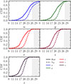 |
Fig. A.1. Cumulative distribution function of the optical magnitudes (u, g, r, i, z) of the galaxies included in the N90 sample (dashed lines). For comparison, we have included the CDF of the true hosts (solid lines). Shaded areas correspond to the magnitudes that LSST cannot detect. |
Appendix B: Strategies for identifying hosts of CGWs with S/N > 25: Galaxy color cuts
In this Appendix, we explore the possibilities of decreasing the number of potential candidates (N90) within the sky-localization area restricted for CGWs detected with S/N > 25. To this end, in Fig. B.1 we present the u − g, g − r, r − i and i − z color distributions. As we can see, the distributions of candidates and true hosts are very different. This is particularly evident when we show in the lower panels of Fig. B.1 the cumulative distribution functions. These differences can be used to perform a color cut and reduce a large number of candidates. To quantify this, we presented Table B.1. As shown, with a cut in the r − i or i − z we can diminish the potential host candidates ∼ 70%. These results suggest that a color-cut is a viable approach for reducing the number of potential host candidates in cases where CGWs are detected with a high S/N.
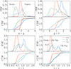 |
Fig. B.1. Color distribution of the galaxies within the sky-localization area (N100, green), galaxies within the galaxies within the sky-localization area contribution to the 90% probability of being the true host (N90, blue) and the true host (Host, red). Upper panel: Cumulative distribution function (CDF) of the u − g, g − r, r − i and i − z colors for N100, N90 and true host. The horizontal black line corresponds to the value where the CDF of the Host reaches 10%. Lower panels: Probability distribution function (PDF) of the u − g, g − r, r − i and i − z colors for the three samples studied. In all the plots, the distributions correspond to the galaxies associated with CGWs whose S/N > 25. |
Fraction of N90 galaxies removed after applying different optical color cuts with LSST filters.
All Tables
Fraction of N90 galaxies removed after applying different optical color cuts with LSST filters.
Fraction of N90 galaxies removed after applying different optical color cuts with LSST filters.
All Figures
|
Fig. 1. Upper panel: Sky distribution of the SKA PTA pulsars (orange) and the MBHBs detected as CGW (blue) within the 200 MBHB realizations. The size of the blue points corresponds to the S/N of the CGW. Lower panel: Right ascension versus redshift for all the galaxies placed in the light cone within a thin slide of 0.1 deg. For the sake of clarity, we only show the z < 0.3 redshift range. |
| In the text | |
|
Fig. 2. Normalized distribution of the sGWB characteristic strain amplitude at f1/10yr. The orange histogram represents the posterior distribution inferred by the EPTA collaboration (EPTA Collaboration and InPTA Collaboration 2023a), while the orange shaded region represents the ±3σ interval. The blue histogram corresponds to the strains produced by the MBHB population generated by L-Galaxies. |
| In the text | |
|
Fig. 3. Upper and middle panels: Observed photometry in LSST for three detected MBHBs (upper panels) and the stellar component of their host galaxies (middle panels). Blue, green, red, purple, and brown dots correspond to the flux inside the u, g, r, i, z filters, respectively. The properties of the binary and the host galaxy are indicated in each panel. Lower panels: Observed SED ( |
| In the text | |
|
Fig. 4. Sky-localization of two different random sources inside our light cones (blue and purple areas). The upper one features a S/N ∼ 6, while the lower one corresponds to S/N ∼ 10. The orange points correspond to the position of the SKA PTA (different from sample to sample as explained in Section 4.2). |
| In the text | |
|
Fig. 5. Upper panel: Distribution of the number of MBHBs resolved by the 30 year SKA (Nres) in each light cone generated by L-Galaxies. Lower panel: Cumulative distribution function of the signal-to-noise ratio for the resolved MBHBs. |
| In the text | |
|
Fig. 6. Properties of the detectable sources by 30 year SKA: Chirp mass distribution (ℳ, upper left panel), redshift (z, upper right panel), twice the observed Keplerian frequency (f2, center left panel), eccentricity (e, center right panel), mass ration (q, lower left panel), and inclination angle (i, lower right panel) of the detected MBHBs. The term NBin represents the number of objects in a given bin of the histogram, while Ntot is the total number of objects analyzed. For reference, we present with black lines the distribution of eccentricity and inclination angle for all the MBHBs presented inside the light cone. |
| In the text | |
|
Fig. 7. Upper panel: Cumulative distribution function of the AGN magnitude associated with the MBHB sourcing the CGWs. Each color corresponds to a different LSST filter: u, g, r, i, z. Dashed vertical lines represent the limiting magnitudes of the LSST in each filter. Lower panel: Cumulative distribution function of the X-ray flux in the soft (0.5–2 KeV, green) and hard X-ray (2–10 KeV, purple) bands. Dashed vertical lines highlight the detection limit of eRosita. |
| In the text | |
|
Fig. 8. Properties of the galaxies hosting the MBHBs sourcing the CGWs detected by 30 year SKA: Galaxy stellar mass (M*, upper left), sSFR (upper right), bulge-to-total ratio (B/T, lower left), and stellar magnitude in the (u, g, r, i, z) set of filters (lower right). In the panel with the sSFR, the vertical line highlights the 10−11 yr−1 value. On the other hand, the blue line corresponds to the cumulative distribution. Finally, the vertical lines correspond to the magnitude limits of LSST in the u, g, r, i, z filters. |
| In the text | |
|
Fig. 9. Histogram and cumulative density function (in blue) of Ω90 of the resolved sources. The light blue area represents the CGW with an Ω90 < 100 deg2 for which we consider for a possible EM follow-up. |
| In the text | |
|
Fig. 10. Distribution in the (RA, Dec, z) space of the galaxies with M∗ > 1010.3 M⊙ and the r-band < 27.5 mag placed within the sky-localization area constrained by SKA PTA. Top panel: Distribution of the galaxies when no probability selection is performed. N100 indicates the total number of these galaxies. Middle panel: Same as top panel but when presenting only the galaxies that contribute to the 90% probability of being the true host (see Section 5). The size of the circle is proportional to the probability. Lower panel: Right ascension and declination plane. The gray (colored) points correspond to all the galaxies in the N100 (N90) sample. The color encodes the photometric color i − z. |
| In the text | |
|
Fig. 11. Number of candidates (Ncand) within the sky-localization area depending on the S/N of the detected CGW source. Green circles correspond to the total number of galaxies with M∗ > 1010.3 M⊙ within the detection area (N100). Blue and orange circles represent the same thing, but only including the galaxies contributing 90% and 50% of the total probability of being the true host. To improve the plot clarity, orange points have been shifted by a factor of 0.5. The gray line corresponds to the expected 1/(S/N)2 relation. |
| In the text | |
|
Fig. 12. Upper panels: Probability distribution function of the u − g, g − r, r − i, and i − z colors for the galaxies within the sky-localization area (N100, green), the galaxies within the sky-localization area contributing to the 90% probability of being the true host (N90, blue), and the true host (Host, red). Lower panel: Cumulative distribution function of the u − g, g − r, r − i, and i − z colors for N100, N90, and true host. In all the plots, the distributions correspond to the galaxies associated with CGWs whose S/N < 25. |
| In the text | |
|
Fig. 13. Color-color diagrams for the galaxies hosting the CGW (Hosts, red circles) and the galaxies inside the sky-localization area contributing to 90% probability (N90, blue contours). In all the plots, the distributions correspond to the galaxies associated with CGWs with S/N < 25. Green circles represent the region where AGNs are expected to be placed in the color-color diagram. |
| In the text | |
|
Fig. A.1. Cumulative distribution function of the optical magnitudes (u, g, r, i, z) of the galaxies included in the N90 sample (dashed lines). For comparison, we have included the CDF of the true hosts (solid lines). Shaded areas correspond to the magnitudes that LSST cannot detect. |
| In the text | |
|
Fig. B.1. Color distribution of the galaxies within the sky-localization area (N100, green), galaxies within the galaxies within the sky-localization area contribution to the 90% probability of being the true host (N90, blue) and the true host (Host, red). Upper panel: Cumulative distribution function (CDF) of the u − g, g − r, r − i and i − z colors for N100, N90 and true host. The horizontal black line corresponds to the value where the CDF of the Host reaches 10%. Lower panels: Probability distribution function (PDF) of the u − g, g − r, r − i and i − z colors for the three samples studied. In all the plots, the distributions correspond to the galaxies associated with CGWs whose S/N > 25. |
| In the text | |
Current usage metrics show cumulative count of Article Views (full-text article views including HTML views, PDF and ePub downloads, according to the available data) and Abstracts Views on Vision4Press platform.
Data correspond to usage on the plateform after 2015. The current usage metrics is available 48-96 hours after online publication and is updated daily on week days.
Initial download of the metrics may take a while.