| Issue |
A&A
Volume 706, February 2026
|
|
|---|---|---|
| Article Number | A73 | |
| Number of page(s) | 25 | |
| Section | Numerical methods and codes | |
| DOI | https://doi.org/10.1051/0004-6361/202556909 | |
| Published online | 03 February 2026 | |
Optimized smoothing kernels for smoothed particle hydrodynamics
Institute of Theoretical Astrophysics, University of Oslo,
Postboks 1029,
0315
Oslo,
Norway
★ Corresponding author: This email address is being protected from spambots. You need JavaScript enabled to view it.
Received:
19
August
2025
Accepted:
1
December
2025
Abstract
We present a set of new smoothing kernels for smoothed particle hydrodynamics (SPH) that improve the convergence of the method without any additional computational cost. These kernels are generated through a linear combination of other SPH kernels combined with an optimization strategy to minimize the error in the Gresho-Chan vortex test case. To facilitate the different choices in gradient operators for SPH in the literature, we performed this optimization for both geometric density average force SPH (GDSPH) and linear-corrected gradient SPH (ISPH). In addition to the Gresho-Chan vortex, we also performed simulations of the hydrostatic glass, Kelvin-Helmholtz instability, Sod shocktube case, and Evrard collapse as well as a subsonic blob test. At low neighbor numbers (<128), there is a significant improvement across the different tests, with the greatest impact shown for GDSPH. Apart from the popular Wendland kernels, we also explored other positive-definite kernels in this paper, which include the “missing” Wendland kernels, Wu kernels, and the Buhmann kernel. In addition, we also present a method for producing arbitrary non-biased initial conditions in SPH. This method uses the SPH momentum equation together with an artificial pressure combined with a global and local relaxation stage to minimize local and global errors.
Key words: hydrodynamics / methods: numerical
© The Authors 2026
 Open Access article, published by EDP Sciences, under the terms of the Creative Commons Attribution License (https://creativecommons.org/licenses/by/4.0), which permits unrestricted use, distribution, and reproduction in any medium, provided the original work is properly cited.
This article is published in open access under the Subscribe to Open model. This email address is being protected from spambots. You need JavaScript enabled to view it. to support open access publication.
1 Introduction
Smoothed particle hydrodynamics (SPH) is a Lagrangian particle method that has been applied to a wide range of topics within astrophysics. The traditional SPH method can be derived from the principle of least action and the Euler-Lagrange equations (Monaghan 1988; Price 2012), resulting in a numerical scheme for hydrodynamics that spatially conserves linear momentum, angular momentum, entropy, and energy exactly and that leaves the error in conservation mainly dependent on the time integration scheme1. Many of the drawbacks of the traditional SPH method, such as handling shocks, shear flow, convergence issues, and density gradients, have been greatly improved over the years. In addition, there are still numerous aspects of the method that remain unexplored, with the potential for even more improvements in the future. In this article we focus on improving the convergence qualities of SPH.
Since SPH is a particle-based method, the fluid is discretized by mass elements rather than volume elements, as in grid-based codes. A smoothing kernel is used to interpolate the fluid quantities at any point in space. This includes the density, which determines the effective volume of the particles. While the sum of volume elements in a grid code remains constant, the sum of particle volumes in an SPH code is highly dependent on the accuracy of the interpolation. This accuracy is mainly determined by the smoothing kernel and how well the particles are distributed within the kernel. An optimally distributed set of particles satisfies, for each particle a, the following constraints:
 (1)
(1)
 (2)
(2)
where the summation runs over neighboring particles, b, with mass mb, density ρb, and kernel weighting function Wab. Here Q0 represent the partition of unity, and Q1 indicates that there is no preferred direction or bias in the distribution of particles. The larger the deviation from these values, the worse the interpolation of fluid quantities. Related to this is the effective area between particles, which is analogous to the flux area between volume elements in grid-based codes. In a grid-based code, the areas fully enclose the volume of the resolution element ( ), where S is the bounding surface of the resolution element and
  is the unit normal vector pointing outward from the surface. However, in SPH this is not necessary true and will again depend on the particle distribution such that there can be a non-canceling of particle areas (
 ). As momentum flux is made to be symmetric in SPH (such that momentum is conserved), non-canceling of particle areas leads to an automatic re-meshing mechanism in SPH. This causes particles to move to minimize this error and move toward a more optimal particle dis-tribution2. This will occur even in the absence of hydrodynamic forces (constant pressure) and has thus come to be known as the zeroth order error of SPH. Particles that are optimally distributed fulfill the cancellation of areas and the following conditions:
 (3)
(3)
 (4)
(4)
Here E0 is the zeroth order error3 and E1 is the linear gradient error. The indices i, j ∈ {x, y, z} denote Cartesian vector components and δij the Kronecker delta. Here we use the GDSPH gradient operator (Wadsley et al. 2017), which we continue to use for the rest of this paper. The momentum equation for SPH is derived from the Euler equations and given by
 (5)
(5)
To get the error terms of this function, we can Taylor expand Pb around ra :
 (6)
(6)
It can be seen that our momentum equation is of the second order if the particle fulfills the E0 and E1 conditions. Most of the time this is not the case, but we can develop optimizations to try and minimize these kinds of errors. These optimization often involve different smoothing kernels, numbers of neighbors, corrections to the gradients, different gradient operators, or different choices of effective particle volume.
Linear-exact gradient corrections have become popular in recent times due to the increased accuracy they offer in subsonic flows and in shearing flows. Here, a matrix inversion of the E1 condition is performed and then applied to the gradient of the kernel to ensure that the E1 condition is fulfilled. There are a few variations to this correction. The most straightforward is to simply invert E1 in Eq. (4) (Bonet 1999; Price & Monaghan 2004). In the CRKSPH formulation (Frontiere et al. 2017) and the SPH method presented by Rosswog (2025), the kernel and its derivatives are reproduced to enforce both the zeroth order and the linear order; however, when deriving the pairwise forces to uphold linear momentum conservation, the zeroth order correction is effectively lost, and only the linear correction remains. There might be benefits in these reproducing kernels over other linear correction methods, but that remains to be seen. Another way of constructing linear-exact gradients for SPH was devised by García-Senz et al. (2012). In their proposal, gradients are calculated from an integral expression so that there is no need to explicitly calculate the analytic derivative of the kernel function. Similarly to Bonet (1999); Price & Monaghan (2004), a matrix inversion is then performed to linearly correct for the gradients. This method is known as the integral smoothed particle hydrodynamics (ISPH) scheme (García-Senz et al. 2012). Integral-based estimates have been readily applied in the past for second derivatives, as they are much less noisy than analytical second derivatives of the smoothing kernel (Brookshaw 1985; Monaghan 2005). Moreover, ISPH have shown great advantages over regular SPH in subsonic flows (García-Senz et al. 2012; Rosswog 2015; Valdarnini 2016). The disadvantages of these linear corrections include the additional computational cost and the discrepancy in errors between the density estimate and velocity gradients, potentially leading to entropy errors. Global angular momentum is also no longer fully conserved in these formulations, as the pairwise force is not always radially aligned between particles. This becomes a resolution-dependent error, and it has been stated to remain relatively small (Frontiere et al. 2017); however, this error is dependent on both resolution and the given particle distribution. On the other hand, this is offset by more precise local angular momentum transport due to more accurate gradients.
The interpolation kernel is the foundation of the SPH method and is ever present in determining the accuracy of a simulation, even when applying the optimizations mentioned above. For a long time, B-splines were the most popular smoothing kernel to use due to their compact support, good interpolation, and flexibility in polynomial degree. However, an issue with these kernels has always been that they are susceptible to the pairinginstability. The pairing-instability occurs when the number of neighbors exceeds a certain critical value, causing particles to clump together and consequently reducing the resolution of the simulation (Thomas & Couchman 1992; Morris 1996; Børve et al. 2004; Price 2012; Dehnen & Aly 2012). This critical value will depend on the kernel, but for the cubic kernel, it lies in the region of Nsmooth = 50. Increasing the number of neighbors leads to more accurate low-order errors (E0, E 1, Q0, Q1) and less particle noise. This is particularly desirable when modeling subsonic flows, where smooth velocity fields are essential4. This is why Wendland kernels have become very popular in recent times, as they are stable against the pairing instability at all neighbor numbers. It was shown in Dehnen & Aly (2012) that a positive Fourier transform is a necessary condition for stability against the pairing instability, though it is still unclear why negative values in the Fourier transform triggers the pairing instability. It has been hypothesized that this is a consequence of the particles trying to re-order themselves in order to minimize the total internal energy (U) given a fixed entropy. While the uniform particle distribution always represents a local minimum, if a paired particle distribution results in a lower internal energy, then the uniform particle distribution is only meta-stable. Cubic spline kernels are hypothesized to exhibit this meta-stable property, as it has an oscillating over-under estimation of density given a uniform particle distribution for varying neighbor numbers. The Wendland kernel and other kernels with positive definite Fourier transform seem to exhibit an overestimation of the density, which continuously decreases as number of neighbors increases. Dehnen & Aly (2012) hypothesized that pairing occurs when the following condition is fulfilled: ρ(Nsmooth/f ) < p(Nsmooth); for 1 < f ≤ 2. The overestimation of the density by the Wendland kernel can be especially high when using low neighbor numbers. Nevertheless, one can correct for the kernel bias by adjusting the self-interaction term (W(0, h)), thus effectively removing this bias from the density estimate while leaving the gradients unaffected. Though the Wendland kernels have been popularized, there are many other interpolation kernels that meet the criteria of having a positive Fourier transform, Gaussian shape, and compact support. These include the Wu family of kernels (Wu 1995), the missing Wendland kernels (Schaback 2011), and the Buhmann family of kernels (Buhmann 1998). Another family of kernels is the Sinc kernels,  (Cabezón et al. 2008; García-Senz et al. 2014), which is directly linked to the Dirac-δ function. Sinc kernels, as with the B-spline family of kernels, can be subject to the pairing instability. However, the critical neighbor number for the instability can be pushed higher by increasing the sharpness of the kernel, which is controlled by the kernel exponent n. A consequence of increasing the sharpness is that it usually gives a worse interpolation at lower neighbor numbers. This is likely related to the larger difference in weight between the inner and outer regions produced by sharper kernels. Recently, a linear combination of two Sinc kernels was proposed by Cabezón & García-Senz (2024) to generate a kernel that is more resistant to the pairing instability while retaining good interpolation properties over a wide range of neighbors numbers. In this work, we aim to design smoothing kernels specifically optimized for SPH rather than using interpolation kernels developed for other purposes. Our approach involves optimizing a linear combination of kernels, similar to the method in Cabezón & García-Senz (2024), to produce the most accurate kernel for a given neighbor number. A big challenge in this work was determining the most natural initial conditions to minimize any kind of bias.
Lattice initial conditions are often used to provide an initially optimal distribution of particles. In this case, particles are put in a cubic or closed package lattice. At first this might seem to be a nice solution, as the E0 and E1 conditions are fulfilled. But there are many disadvantages to actually using a lattice for the initial condition. First, the lattice structure is easily broken by shocks and shear flows, which will generate aggressive noise as the particles move off the lattice structure, and this will cascade through the simulation volume. Second, particle lattice distributions can introduce directional bias and simulation artifacts. For instance, a shock wave propagating along a preferred direction of the lattice can disproportionately gather particles in that direction, leading to undesirable oscillations. Third, the two issues above are exacerbated when dealing with density gradients in the initial conditions. Lattice particle distributions can give both an artificial positive result for SPH, as it provides very high accuracy as long as the lattice holds up, but also an artificial negative result, as significant noise is generated when the lattice breaks down. A much more natural distribution for SPH is the glass distribution, which SPH will always strive to re-mesh toward as particles are disturbed by such forces as shocks and shear flows. Glass distributions are often obtained by letting the particles relax, beginning with a lattice or random distribution, adding some random velocities, and using a velocity damping term to eventually approach a steady state. This can be done with the influence of gravity to generate collapsed density structures or without it to generate uniform distributions. However, this method has limitations and downsides. First, one cannot generate density contrasts for setups that are purely hydrodynamic5 (the Kelvin-Helmholtz setup for example). Second, glass generation performed in this way can be costly, as oscillations can take a long time to damp. Third, damping the velocities too quickly can lead to inaccurate distributions. In this paper, we have instead developed a glass generator that relies on the SPH method to find a relaxed glass distribution for arbitrary density gradients.
The use of lattice initial conditions is especially problematic when it comes to assessing the quality of a smoothing kernel, as the results do not reflect the natural distribution of particles and give a positive bias toward smoother kernels, which usually have larger E0 errors in glass distributions (given the same neighbor count). In Dehnen & Aly (2012), the correction for the kernel bias was made based on the bias when interpolating a closed-packed lattice distribution. The bias was also given by a simple power law. In this paper we calculate a new correction to the kernel bias for all our kernels that is based on the generated glass that each kernel itself produces. We also give a piecewise function to capture the kernel bias more accurately over a wider-range of neighbor numbers.
In Sect. 2 we present all the smoothing kernels used in this paper. In Sect. 3 we go through the methods used in this paper, including the SPH methods, the IC generator, adjustment of density bias, and the optimization strategy. In Sect. 4 we present the results from the tests. And finally in Sect. 5 we discuss our results.
2 Kernel properties
All the kernels we go through in this section go to zero at
 (7)
(7)
even if not stated explicitly in the equations. All kernels are normalized with
 (8)
(8)
A useful tool for analyzing kernels is their Fourier transform. Despite having similar shapes, kernels can exhibit quite different Fourier transforms. As previously mentioned, negative values in the Fourier transform are responsible for the pairing instability. The lower the wave numbers at which these negative values appear, the lower the critical number of neighbors required to trigger this instability. The Fourier transform is defined as
=4\pi k^{-1} \int_0^{\infty} \sin(kr)W(r)r{\rm d}r,](/articles/aa/full_html/2026/02/aa56909-25/aa56909-25-eq13.png) (9)
(9)
where W(r) is the smoothing kernel and k is the wave number. All the kernels that we mention in this section are positivedefinite, which means that they have as strictly positive Fourier transform. Positive definite kernels all produce a general overbias in their density estimation, which become more prominent at low neighbor numbers, as the bias is dominated by the self contribution. The neighbor number at which this bias becomes negligible depends on the smoothing kernel (higher order/more peaked kernels give higher bias). This self contribution can be corrected for as described in Sect. 3.3.
2.1 Generalized Wendland kernel
The Wendland kernels is a family of compactly supported radial functions generated by a dimension walk (integration) of a truncated power function (Wendland 1995).
 (10)
(10)
Here k is the smoothness parameter, l(k) is the order of the kernel, and  is the floor operator. We set l(k) so that the generated function is strictly positive definite and radial on R3 (following D ≤ 2l - 1 for D dimensions). The Wendland kernels produce the minimal polynomial degree for a given space dimension and smoothness. While initially only determined for positive integer smoothness parameters, this property has been generalized for non-integer smoothness parameters in the generalized Wendland functions (Chernih & Hubbert 2014):
![Mathematical equation: \begin{multline} \phi_k(r) = \frac{\Gamma[l(k) + 1]}{2^{l(k) + k} \Gamma[l(k) + k + 1]} \left(1 - r^2\right)^{l(k) + k} r^{-l(k)} \\ \times \, {}_2F_1\left(\frac{l(k)}{2}, k + \frac{l(k) + 1}{2}, l(k) + k + 1, 1 - \frac{1}{r^2}\right). \end{multline}](/articles/aa/full_html/2026/02/aa56909-25/aa56909-25-eq16.png) (11)
(11)
Here Γ is the gamma function and 2F1 is the hyper-geometric function. The family of Wendland kernel functions for 3D is then defined as
 (12)
(12)
Positive integers of k represent the classic Wendland kernels, where the resulting kernels have polynomial structure. The Wendland kernels with positive integers used in this paper (k = 0,1,2,3) are
 (13)
(13)
 (14)
(14)
 (15)
(15)
 (16)
(16)
Positive half-integers are known as the missing Wendland kernels (Schaback 2011). They are compactly supported and polynomial but with additional logarithmic and square-root terms ( k = 0.5):
 (17)
(17)
Positive non-integer kernels can also be generated; these involve a more complicated form (k = 0.4):
 (18)
(18)
To avoid handling hyperbolic functions within our code we approximate this function with a polynomial fit. Higher-order kernels have smoother derivatives, which in combination with higher neighbor numbers act to decrease the sensitivity to particle disorder. The trade-off of using a higher-order kernel is that it becomes less accurate than its lower-order counterpart at low neighbor numbers (Monaghan 1992; Rosswog 2015). We refer to the Wendland kernels as C2, C4, C6, CM05, and CM04 throughout this paper.
2.2 Wu kernel
The Wu approach starts with the function (Wu 1995)
 (19)
(19)
Another function is then generated by convolution:
 (20)
(20)
Using this function, the Wu family of kernels is generated by dimension walk (derivative):
 (21)
(21)
The Wu kernel (φl,k) is strictly positive definite and radial in Rd for D ≤ 2k + 1, with polynomial of degree 41 - 2k + 1 and smoothness of C2(l-k), which indicates how many times the kernel is continuously differentiable (2(l - k) times). The polynomial degree is higher for the Wu kernel than the Wendland kernel at a certain smoothness. In this paper we have chosen to look at the φ1,2 and φ1,3:
 (22)
(22)
 (23)
(23)
For a prescribed smoothness the polynomial degree of Wendland kernels are lower than that of Wu kernels. An interesting thing about Wu kernels is that their Fourier transform is positive, decays quickly, and goes to zero in periodic intervals. We refer to the Wu kernels as WU2 and WU4 throughout this paper.
2.3 Buhmann kernel
Buhmann’s approach (Buhmann 1998) involves integrating a positive function f(t) = tα(1 - tδ)ρ+ against a strictly positive definite kernel  . Buhmann’s family of kernels thus take the general form
 (24)
(24)
Here 0 < δ ≤ 0.5, ρ > 0.5 and the kernel is strictly positive and radial in RD ≤ 3 for λ ≥ 0 and  . Buhmann’s family of kernels consists of a polynomial and an additional logarithmic term. The Buhmann kernel that we include in this paper is (α =
  ρ = 1 λ = 2 from Buhmann 2003):
 (25)
(25)
We refer to this kernel as BUH throughout this paper.
3 Method
3.1 SPH methods
We performed the optimization using both the GDSPH and ISPH methods. We did this because the “best” kernel may differ between the two methods due to the removal of the linear error term. The density of both GDSPH and ISPH was calculated using the standard density estimate
 (26)
(26)
We used the same artificial viscosity scheme for all the simulations. To keep things as simple as possible, we implemented a classic SPH artificial viscosity (Monaghan 1992) with constant α and β. We used α = 1 and β = 2 for the shock cases (Sod-shocktube and Evrard collapse), and for the subsonic cases (Gresho-Chan, Kelvin-Helmholtz, and the subsonic blob test) we used α = 0.05 and β = 2.
3.1.1 GDSPH gradient
We implemented the GDSPH gradient operators of Gasoline2 (Wadsley et al. 2017) in this paper. This variant of SPH is identical to regular SPH when the density is uniform, but it improves gradient accuracy in cases involving sharp density gradients. The momentum equation and internal energy equation in GDSPH is written as:
![Mathematical equation: \frac{{\rm d} \mathbf{v}_a}{{\rm d}t} = - \sum_b m_b \left[ \frac{f_a P_a+f_b P_b}{\rho_a\rho_b} \overline{\nabla_a W_{ab}} \right],](/articles/aa/full_html/2026/02/aa56909-25/aa56909-25-eq35.png) (27)
(27)
 (28)
(28)
Here, fa are entropy correction terms to remove the linear entropy error caused by a mismatch between GDSPH operators and the density estimate (see Wadsley et al. 2017).
3.1.2 Integral based gradient
In ISPH (García-Senz et al. 2012), the gradients are calculated from an integral expression so that there is no need to explicitly calculate the analytic derivative of the kernel. The kernel gradients are also linear-corrected by the use of a matrix inversion of the E1 error. Effectively, we replace the kernel gradients of Eqs. (27) and (28) with ( ):
):
 (29)
(29)
 (30)
(30)
where j is either a or b.
 (31)
(31)
 (32)
(32)
The linear correction matrix, C, is calculated with
 (33)
(33)
This form is slightly different than the one proposed by previous authors(García-Senz et al. 2012; Rosswog 2020). This is because it involves the symmetric kernel  within the linear correction matrix, instead of the one-sided kernel gradient
  . The momentum and internal energy equations become
![Mathematical equation: \frac{{\rm d}\mathbf{v}_a}{{\rm d}t} = - \sum_b m_b \left[ \frac{ P_a \overline{G_{a}^k}+ P_b \overline{G_{b}^k}}{\rho_a\rho_b} \right],](/articles/aa/full_html/2026/02/aa56909-25/aa56909-25-eq45.png) (34)
(34)
 (35)
(35)
This matrix inversion requires us to do an extra neighbor loop and requires us to save six additional quantities per particle (symmetric matrix). This linear correction can introduce a global angular momentum error as pairwise torques can be generated between particles. This is because the forces between particles are no longer ensured to be aligned along the line connecting particles. This is in general true for any kernel correction of order greater than zero. This effectively results in a resolution/kernel dependent error in global angular momentum conservation.
3.2 Initial condition: Glass generator
As discussed in the introduction, producing natural and nonbiased initial conditions are important for SPH. Of particular difficulty is the generation of non-uniform density distributions. Lattice initial conditions can be used in non-uniform density distributions, by either varying particle mass (Lombardi et al. 1999) or stretching a uniform lattice (Rosswog 2009; Price et al. 2018). The main issue with these methods are the use of the lattice initial condition, which as discussed are artificial, biased and experience excessive noise when the lattice breaks. Varying particle masses are undesirable as well, due to particles having more difficulty in balancing the particle distribution and generally leading to larger gradient errors and noise. In Diehl et al. (2015) a more general initial condition generator is proposed, using the concept of weighted Voronoi tessellation. This works well in generating non-uniform density distributions. The main issue with this approach is that the generated distribution does not necessarily correspond to the same natural particle distribution that a given SPH method would produce, as it does not take into account the smoothing kernel or the gradient operators. This means that it will also represent a slightly biased initial condition. In Rosswog (2020), a more SPH-like version of this method is applied, where the SPH momentum equation is used, together with an artificial pressure based on the current density error. This is an excellent approach for generating non-biased initial conditions for SPH, as it ensures a near noise free distribution at the start of your simulation (as one is using the same momentum equation to evolve the system). We propose a similar method in this paper, but add some important alterations to ensure that both local and global errors are minimized. In addition, this method will relax to a given density profile, no matter what your starting initial condition is (given that the mass of the system is correct). Similar to Rosswog (2020), we used an iterative method where during each iteration, i, we updated the position directly for each particle:
 (36)
(36)
The displacement of each particle is determined by the following equations:
 (37)
(37)
 (38)
(38)
The term Kglobal,i will determine the largest multiple of the smoothing length that a particle can be displaced. The variables  and ρi are calculated with the chosen density estimate and gradient operator (in this paper GDSPH (Eq. (27)) and ISPH (Eq. (34))). Hence the produced glass will represent the relaxed distribution of the chosen gradient operator, smoothing kernel and neighbor number. The pressure in the momentum equation is replaced by an artificial pressure given by
 (39)
(39)
Here ρtar is the target density at the current position and ρa is the estimated density for the particle (Eq. (26)). Higher n means that fitting to the density is more important than balancing the particle distribution, that is, reducing E0. This is because a minimization in density error does not necessary mean a minimization in E0. As such, density errors and particle distribution errors will drive the particles into a position that minimizes these errors, just as the case for SPH naturally6. The term Kglobal,iis adjusted after each step following the instructions outlined below:
If the step leads to an overall worse mean
 , then decrease
  .
.If the step leads to an overall better mean
 , then increase
  .
.Relaxation requires that d1 > d2 > 1.0. We set d1 = 1.8 and d2 = 1.1 during the global relaxation and d1 = 1.1 and d2 = 1.002 during local relaxation.
The global relaxation stage quickly reduces the step size to interparticle size to get a good gradient estimate of the current global density profile. The step size is then increased again to a factor of the initial (Cloop,nKglobal,0). Here we set Cloop,0 to 0.5 and reduce it by half each time Cloop,n = 0.5Cloop,0 if there is no improvement to the global density error. If one starts from an IC that captures the global IC well, then this step is not necessary, and only local relaxation is needed.
In the local relaxation stage, which occurs when global relaxation stage is finished, the Kglobal,i in Eq. (37) is near the average interparticle scale. From here on we slow down the rate of relaxation to ensure a more accurate local particle distribution. We stop the IC generator when max(∆ra/ha) < 2 ∙ 10−3, at which point particle motions are negligible, and we consider the distribution relaxed.
The initial value of Kglobal,i is a parameter that can be chosen, but by default it is set to half the system size, as this ensures that the desired density profile is obtained regardless of the input IC. A much lower value can be used if one has an IC that is close to the desired density profile.
Results from the IC generator in the case of the ∆ρ = 8, nx = 64, Nsmooth = 64 Kelvin-Helmholtz IC of Sect. 4.3 can be seen in Fig. 1. From this we can see that we have a proper glass structure in the particle distribution that follows the analytical density profile very closely. As different relaxed glasses will be produced by different smoothing kernels and neighbor numbers, we run the relaxation process for each new kernel and neighbor number when generating ICs in this paper.
3.3 Adjusting density bias
Before we optimized our linear combined kernel, we adjusted the self-bias of all our kernels. This mainly effects the density, giving us a corrected density estimate:
 (40)
(40)
This density correction is a constant and is applied uniformly to all particles. We adjust e so that the density of a relaxed hydrostatic glass is as close as possible to ρ = 1.0 (given that Mtot/Vtot = ρ = 1.0) for a wide range of neighbor numbers. A uniform glass produced by the IC generator will locally be independent of the resolution and only be a function of the number of neighbors and the given kernel. As such we can run low resolution cases with our IC generator and adjust the kernel bias until we produce a glass with a mean density error of around ρerr ≈ 10−5, which is much less than the general SPH density noise. We run this for a wide range of neighbor numbers (Nsmooth ∈ {16,24,32,48,64,96,128,256,512}). After 512 neighbors, the kernel bias is set to 1. We could then interpolate between ranges using a linear piecewise function to correct the kernel:
 (41)
(41)
Here, ci is the e value at Nsmooth = Nmin,i. This was performed for both GDSPH and ISPH. The coefficients and neighbor number can be found in Table B.1 for GDSPH and Table B.2 for ISPH.
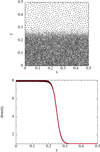 |
Fig. 1 Relaxed glass IC generated by the IC generator outlined in Sect. 3.2. Here we model the IC of the Kelvin Helmholtz instability (Sect. 4.3), with a density contrast of ∆ρ = 8. Top : particle distribution within a thin slice of thickness ∆ z = 0.015. Bottom : density profile in the y direction. The red line depicts the analytical density profile and the black dots the density of the particles. The glass generated density profile is in excellent agreement with the analytical solution. |
3.4 Optimization strategy
In this method, we generate a new kernel by linear combination:
 (42)
(42)
Here, αi and αi + 1 are the coefficients that we optimized for. The process starts with i = 1 and an initial kernel Wnew,0. After determining αi, αi + 1 by minimizing some cost function, we generated a new kernel (Wnew,i). We then repeated this process with the newly generated kernel and two other kernels. This iterative process continued until we used all the kernels that we wished to include in our linear combination. We used the differential evolution method to find the global minimum of the two parameters for each iteration. We set the initial parameter value to (αi,αi+1) = [0.0,0.0], and we set the minimum and maximum parameter boundaries to be bnds = [(−3.0, 3.0), (−3.0,3.0)].
After the optimization was completed, we fit the linearcombination of kernels to a polynomial in the form
 (43)
(43)
 (44)
(44)
During the work of this paper we used two different cost functions and two different cases to optimize the kernel for. These are described in the sections below.
3.4.1 Optimized for hydrostatic glass
Perhaps, one of the simplest cases to determine the quality of a smoothing kernel comes from it’s ability to generate a hydrostatic glass that minimizes the leading errors of SPH. The hydrostatic glass models a homogeneous system in pressure equilibrium. A cubic box with length L = 1 and total mass Mbox = 1 is setup. Particles are randomly distributed throughout the box. Due to the inherent re-meshing property of SPH, the particles will be reorganized to a glass-like structure by the low order errors (Eqs. (3) and (4)). At some point the distribution will be organized into a relaxed glass, where the errors have been minimized (there is minimal/oscillatory change in the mean errors from this point onward). The distribution and the magnitude of the errors in this final relaxed state will depend on both the smoothing kernel, number of neighbors and the SPH method. The leading order error (E0) will locally be independent of the resolution (for uniform density), so we use a relatively low resolution of N = 323 particles. We hypothesized that the relaxed glass with the smallest errors/noise would provide the best result in dynamic cases as well. We defined our cost function for this case as
 (45)
(45)
Here E0 and E1 are given by the norm of the error vectors defined in (Eqs. (3) and (4)) respectively. The term δρerr is given by
 (46)
(46)
Each kernel has had its self-bias adjusted, so that ρmean will be within 10−5 of ρ = 1.0, for their respective glass and kernel (see Sect. 3.3), such that we accurately measure the density noise. We only optimized this case with the GDSPH formula, and we refer to these kernels as Oglass,Nsmooth (Nsmooth = 32, 64, 128, 256) for the rest of the paper. The resulting polynomial coefficients for the optimization are given in Table C.1.
The kernel function, its derivative and its Fourier transform can be seen in Fig. 2 for the optimized hydrostatic glass kernels together with WU2, BUH, CM04, CM05 kernels. All the optimized kernels for different Nsmooth look very similar to each other, and they are a bit steeper than the WU2 kernels. However, some differences can be seen in the Fourier transform, where Oglass,32 has quite a flat trend (similar to BUH kernel), the higher Nsmooth kernels experience stronger oscillations (behavior somewhere in-between the WU2 kernel and the BUH kernel). Even though we allow for the linear combination to result in negative Fourier transforms, we only end up with one kernel that has negative Fourier transform in the high wave number regime (Oglass,64). The performance of these kernels are discussed more in the next section.
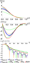 |
Fig. 2 Top : optimized kernel functions for a glass distribution (Sect. 3.4.1) together with the missing Wendland kernels (CM04, CM05), the Buhmann kernel (BUH), and the Wu kernel (WU2). Middle : corresponding derivative of these kernel function. Bottom: fourier transform of these kernels, scaled by k/10. The optimized kernels are quite similar, with some small variations being seen in the Fourier transform. The Oglass,32 kernel deviates the most from the other kernel, with less deep troughs in the Fourier transform. These kernel’s generate excellent glass distributions but degrade significantly in dynamical simulations. |
3.4.2 Optimized for Gresho-Chan vortex
Initially, we assumed that a smoothing kernel with minimal errors in its final relaxed glass state would also yield the best results in dynamic simulations, but this turned out to not be the case. As different kernels have different sensitivity when it’s glass gets disturbed. This was clearly seen when testing out the Gresho-Chan vortex test case. Here, even though the density is uniform, the particle distribution is continuously disturbed by a shear flow.
The Gresho-Chan vortex simulates an inviscid fluid vortex in force equilibrium (Gresho & Chan 1990). The setup is as follows: We setup a 3D thin periodic box with length  , here nx is the average number of particles in the x direction, and the z boundary is set to be roughly 24 particle spacings. The pressure profile is setup following
 (47)
(47)
and the velocity profile follows
 (48)
(48)
Even though conservation of angular momentum within SPH is near exact, the test is challenging for SPH due to the artificial viscosity induced by the particle noise and the errors in the linear gradient (Eq. (4)). The artificial viscosity will cause angular momentum transport, which will lead to mass accretion toward the center and a loss in kinetic energy. Increasing the number of neighbors (Read & Hayfield 2012; Rosswog 2015), using artificial viscosity switches (Cullen & Dehnen 2010), and doing linear gradient corrections (García-Senz et al. 2012; Valdarnini 2016; Cabezón et al. 2017) all improve the convergence of this case.
While testing the Gresho-Chan vortex we found that only Oglass,32 outperformed the other kernels for the Nsmooth it had been optimized for, while all the other Oglass kernels performed rather badly (can be seen in Fig. 5). Similarly, we saw bad result for all kernels that exhibit strong oscillatory behavior in their Fourier transform, such as the WU2 kernel (Fig. 2). Therefore we decided to additionally optimize kernels based on results from the Gresho-Chan vortex following the procedure laid out in the previous sections. The main difference is the cost function, which we set to be the L1,error at t = 1:
 (49)
(49)
 (50)
(50)
Here  stands for the analytical, and
  is the result from the simulation. Similarly to all other setups, we used the IC generator (Sect. 3.2) to generate an initial glass for each kernel and neighbor number before each run. We optimize both GDSPH and ISPH for this case; here the kernels optimized with GDSPH are given by ONsmooth and with ISPH OI,Nsmooth, which was done for Nsmooth = 32, 64, 128, 256. The kernels and the resulting coefficients that were used for the optimization are given in Tables C.2 and C.3.
The kernel function, its derivative and its Fourier transform can be seen in Fig. 3 for the optimized kernels together with C2 and C4 kernels. All the resulting kernels have similar amplitude and form as the Wendland C2 kernel (except for OI,32), but with a minima in its derivative being a bit offset from the C2 kernel. Looking at the Fourier transform we can see quite a clear trend with both the ONsmooth and OI,Nsmooth as we increase Nsmooth ∙ Both O32 and OI,32 drop the fastest within k ∝ 0 - 3π but remain higher than the other kernels as we go to larger wave numbers. As we increase Nsmooth we have a higher power between k ∝ 0 - 3π but lower for higher wave numbers. We have two resulting kernels with regions of negative Fourier transform. The OI,32 kernel, which goes negative in the region k ∝ 4 - 5π, and becomes susceptible to the pairing instability as we go to higher Nsmooth (we see instability at Nsmooth = 128 and Nsmooth = 256). The O256 also has regions of negative Fourier transform at much higher wave numbers (k ∝ 10 - 12π). However, we did not see any sort of instability occurring in this kernel, at least up to Nsmooth = 512. The performances of these kernels are discussed more in Sect. 4.
4 Results
In the following section we discuss the performance of these optimized smoothing kernels on a select number of test cases. First we go through the hydrostatic glass and the Gresho-Chan vortex, both of which we outlined and used for optimization of the kernels in Sects. 3.4.1 and 3.4.2. We then go through four additional tests to see how well the optimized kernels perform in general by testing the Kelvin-Helmholtz instability for two different density contrasts (∆ρ = 2, ∆ρ = 8), the classic Sod shocktube test, Evrard collapse and the subsonic blob test. The hydrostatic glass and Gresho-Chan vortex are run for all the optimized kernels. The ones optimized to hydrostatic glass with GDSPH: Oglass,32, Oglass,64, Oglass,128, Oglass,256. The ones optimized for Gresho-Chan vortex with GDSPH O32, O64, O128, O256 and with ISPH OI,32, OI,64, OI,128, OI,256. We also compare with a select number of kernel’s mentioned in Sect. 2 (CM04, WU2, BUH, CM05, C2, C4, C6). This is done for Nsmooth = 32,64,128,256. For the Kelvin-Helmholtz instability, Sod shocktube, Evrard collapse and subsonic blob test we compare the best-performing kernel at a given Nsmooth with the popular Wendland C2 and C4 kernel, for both GDSPH and ISPH. The optimized kernels was implemented in both the Gasoline2 code (Wadsley et al. 2017) and the ChaNGa code (Menon et al. 2015). Results are from simulations performed with Gasoline2, but we have also confirmed that ChaNGa gives the same results in many of these cases.
4.1 Hydrostatic glass
The setup of this test case is outlined in Sect. 3.4.1. The system is evolved for a long enough time to reach a relaxed glass state. The quality of the resulting glass is quantified with the SPH errors (E0 Eq. (3) E1 Eq. (4)) and the density error (Eq. (46)). These are given for all kernels and chosen neighbor numbers in Fig. 4. While the kernel’s optimized for the hydrostatic glass perform in average the best considering the cost function (Eq. (45)), we can see that it loses out to some other kernels for specific errors. All the GDSPH optimized kernels for the Gresho-Chan vortex perform fairly well, similar to the BUH, CM05 and C2 kernel for the δρerr and E0 error. The O kernels does in general have smaller E1 errors than the standard kernels. The only exception is the O32 kernel that has higher E1 error but has the smallest density and E0 error out of all the kernels for N32. The WU2 kernel performs very well for higher neighbor numbers and is close to the results of the optimized kernel Oglass,128 and Oglass,256. The biggest improvement that can be seen when comparing the Oglass and O kernels with the Wendland C2 kernels, is in the E1 errors that are significantly reduced. We can see that the OI,32 kernel performs very badly when relaxing to a hydrostatic glass with the GDSPH gradient operator, even at Nsmooth = 32. This is, however, not the case when relaxing with ISPH at Nsmooth = 32, indicating that glass relaxation is different when using ISPH.
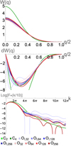 |
Fig. 3 Top : optimized kernel functions for the Gresho-Chan vortex (Sect. 3.4.2), for both GDSPH and ISPH together with the popular Wendland kernels (C2, C4). Middle : corresponding derivative of these kernel function. Bottom : fourier transform of these kernels, scaled by k/10. The optimized kernel exhibit a clear trend in it’s Fourier transform, where the kernels optimized for higher Nsmooth emphasizes lower power beyond k > 3π. The general form of the optimized kernel is quite similar to the Wendland C2 kernel. In general GDSPH produces lower power than ISPH in the high wave number regime for a given Nsmooth. The OI,32 kernel is the only optimized kernel that exhibits a negative Fourier transform at low wavenumbers. Among the other optimized kernels, only O256 has a negative Fourier transform, but this occurs at higher wavenumbers and remains stable to pairing instability up to at least Nsmooth < 500. |
 |
Fig. 4 Relative increase or decrease of the δρerr (top), E0 (middle), and E1 (bottom) of the hydrostatic glass when relaxed for different kernels in respect to the corresponding error of the C2 kernel. The simulations here were performed with only the GDSPH method. The terms N32, N64, N128, and N256 refer to the number of neighbors: Nsmooth = 32,64,128,256, respectively. The δρerr, E0 and E1 of the C2 kernel for each Nsmooth is δρerr = 5.539 × 10−3,3.747 × 10−3,1.243 × 10−3,5.860 × 10−4, E0 = 2.763 × 10−3,2.024 × 10−3, 6.797 × 10−4,4.253 × 10−4, and E1 = 2.210 × 10−2,1.484 × 10−2,2.557 × 10−3,8.305 × 10−4. The optimized kernels can in general be seen to drastically reduce the E1 error relative to the C2 kernel. For the glass optimized kernel’s we can also see a general decrease in both δρ and E0 for their given Nsmooth. |
 |
Fig. 5 Relative increase or decrease of the L1,error of the Gresho-chan vortex at t = 1 and nx = 64 for different kernels in respect to the L1,error of the C2 kernel. The terms N32, N64, N128, and N256 refer to the number of neighbors: Nsmooth = 32,64,128,256. Left : simulations done with the GDSPH method. Right : simulations done with the ISPH method. The L1,error of the C2 kernel for each Nsmooth is L1,error = 1.49375 × 10⁻¹, 9.57342 × 10⁻², 4.70888 × 10⁻², 2.99816 × 10⁻² for GDSPH and L1,error = 9.34635 × 10⁻², 4.66192 × 10⁻², 2.64744 × 10⁻², 2.22268 × 10⁻² for ISPH. An improvement for the optimized kernel at a given Nsmooth across all Nsmooth can be seen for both methods, where the biggest improvements are for the N64 and N128 for GDSPH and N32 and N64 for ISPH. Of the non-optimized kernels, we observed that the C2 kernel performs best, except for Nsmooth = 32 (GDSPH), Nsmooth = 32,64 (ISPH), where CM05 performs better and C4 performs slightly better at Nsmooth = 256 (ISPH). |
4.2 Gresho-Chan vortex
The setup of this test case is outlined in Sect. 3.4.1. We run the Gresho-Chan vortex up to t = 3. We also perform a convergence study, to see if the optimized kernels still perform well as we increase/decrease the resolution, as the optimization was performed at nx = 64 resolution. For this convergence study we only compare with the Wendland C2 and C4 kernels. The optimization of the ON smooth kernels was done at t = 1, we can see the result of the L1,error (see Eq. (50)) at t = 1 in Fig. 5 for both GDSPH and ISPH. From this table we can see that the optimized kernels for the Gresho-Chan vortex perform the best for their given Nsmooth. The difference in L1,error is more pronounced for lower Nsmooth and for the GDSPH method compared to the ISPH method. A comparison of the azimuthal velocity structure (nx = 64, t = 3) between the optimized kernel and the Wendland C2 and C4 kernel can be be seen in Fig. 6 for GDSPH and ISPH. For GDSPH we can see that the optimized kernel mitigates the decay of the vortex structure (in particular for Nsmooth = 64). For ISPH the effect of the optimized kernels can mainly be seen as less noise in the vortex structure, while the general decay is similar across all the kernels (as this is highly dependent on the linear gradient estimate). A convergence study at t = 3 of the L1,error can be seen in Fig. 7 for GDSPH and Fig. 8 for ISPH. Looking at the convergence study, we can see that the improvement of the optimized kernels in general stays true for higher and lower resolution.
Looking at the GDSPH results, we can see that while the O128 kernel proved to be the best at t = 1, this is no longer true at t = 3 and Nsmooth = 128, where the O256 performs better across all resolutions at this time. And looking at the result at the earlier time of t = 1, the O128 just barely performed better at Nsmooth = 128 nx = 64, but worse than O256 for higher resolution. We can also see that the O256 performs better than the O64 at Nsmooth = 64 for the higher resolutions(nx = 128, 256) at both t = 1 and t = 3. The improvement seen in Nsmooth = 64 for GDSPH is the largest improvement that we see in across all our Gresho-Chan cases, where the optimized kernels effectively half the L1,error compared to the Wendland C2 and C4 kernels, resulting in errors similar to Nsmooth = 128 errors of the Wendland kernels (at both t = 1 and t = 3). This is quite clearly seen in Fig. 6, when comparing the O64 Nsmooth = 64 vortex structure with the Nsmooth = 128, C2 and C4 vortex structure. A quite surprising result is that the C4 kernel performs better than the C2 kernel for Nsmooth = 64, while performing worse for Nsmooth = 32,128, where at Nsmooth = 32 it performs drastically worse. For Nsmooth = 32, we can see that the C2 kernel performs relatively well, but with O32 being about a 20-30% improvement at t = 1 and the only kernel with some sort of vortex structure at t = 3 (as can be seen in Fig. 6).
Looking at the result from ISPH, we can see a much less difference between all the different kernels, especially at high neighbor number (Nsmooth = 128,256). At t = 3 and Nsmooth = 256 we can see that the C4 kernel actually performs better than all other kernels, including the optimized kernel OI,256. This is quite surprising, as the OI,256 performs better at earlier times, and looking at the E0 errors at t = 3 in Fig. 9, we can see that they are higher for C4 compared to all other kernels. This likely means that C4 has smaller higher order errors, compared to the other kernels. The OI,32 kernel performs significantly better than all the other kernels at Nsmooth = 32 and is the only optimized kernel with negative Fourier transform at relatively low wave number, which means that it becomes unstable to pairing instability at higher neighbor numbers (above Nsmooth = 64). The Wendland C4 kernel is by far the worst kernel at lower neighbor numbers (Nsmooth = 32,64) for ISPH. For Nsmooth = 64 at both t = 1 and t = 3, the OI,64 produce a significant improvement compared to the Wendland kernels.
The convergence scaling seems to be similar between kernels, but with some experiencing a flattening at higher resolution. The C4 kernel seems to scale a bit better than other kernels at higher resolution, though still being worse in general. The scaling will also depend on the given dissipation scheme/parameters used. We have also run the Gresho-Chan vortex with different dissipation parameters (α = 0.01,0.05,0.1) and the relative results seen in this section remains the same.
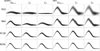 |
Fig. 6 Azimuthal velocity in the radial direction of the Gresho-Chan vortex at t = 3. Here the resolution is nx = 64 and simulation was performed with GDSPH (left three columns) and ISPH (right three columns). We compare the optimized kernel at a given Nsmooth to the popular Wendland C2 and C4 kernels, and vary the number of neighbors in each row (Nsmooth = 32,64,128,256), referred here to N32, N64, N128, N256. The solid black line show the analytical solution and the black dots show the results from the simulation. The X axis (cylindrical radius) extends from 0.0 to 0.7, and the vertical extent from the top to the bottom of the analytical solution is 1. We can see a significant improvement in the optimized kernels for the GDSPH method for Nsmooth = 32,64,128, where the vortex structure becomes more pronounced. Overall less noise can be seen for all Nsmooth. The ISPH method captures the overall vortex structure well for all Nsmooth, due to exact linear gradients. But we can see significant improvement in the noise level of the optimized kernels, compared to the C2 and C4 kernels. |
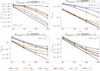 |
Fig. 7 Convergence study of the Gresho-Chan vortex with the GDSPH method for Nsmooth = 32,64,128,256. Here we plot the L1,error over resolution elements in the x direction (nx) at t = 3. Significant improvements can be seen for all optimized kernels compared to the Wendland C2 and C4 kernels. The kernels were optimized in respect to an earlier time t = 1 and we can see that O256 have an improved result over O128 for Nsmooth = 128 at this later time, even beating out O64 for Nsmooth = 64 at higher resolution (nx > 128). The C4 kernel exhibits slightly better convergence slope at high Nsmooth and nx > 128, likely due to it’s higher order properties (fewer O(h2) errors). |
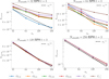 |
Fig. 8 Convergence study of the Gresho-Chan vortex with the ISPH method for Nsmooth = 32,64,128,256. Here we plot the L1,error over the resolution elements in the x direction (nx) at t = 3. Significant improvements can be seen for the optimized kernels at Nsmooth = 32,64 compared to the Wendland C2 and C4 kernels. While at higher Nsmooth, there is much less difference between all the kernels. The kernels were optimized in respect to an earlier time, t = 1, and we observed that C4 performs better at this later time for Nsmooth = 256 than all the optimized kernels at all resolutions. This is surprising, as E0 errors of the optimized kernels are much lower than the C4 kernel (see Fig. 9), which might indicate that long-term behavior at this Nsmooth is heavily determined by the higher order errors (O(h2)). |
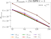 |
Fig. 9 Convergence study of the Gresho-Chan vortex with the ISPH method for Nsmooth = 256. Here we plot the E0 error versus the number of resolution elements in the x direction (nx) at t = 3. Much lower zeroth order errors for the optimized kernel and C2 kernel can be seen compared to the higher order C4 kernel. Note here that even though being zeroth order (dependent on local particle order), the error still decreases with increasing resolution ( |

4.3 Kelvin Helmholtz
The Kelvin-Helmholtz (KH) instability occurs when there is a shearing flow between two fluid interfaces. The instability quickly generates a series of rolling waves at the interface between the two fluids, which eventually breaks down into turbulence, mixing the two fluids. The instability plays a significant role in all kinds of fluids and is a crucial component for any hydrodynamical code to model, as it effectively allows two fluids to mix and generate turbulence. However, traditional SPH methods have been known to struggle with triggering the KH instability, particularly when there are significant density contrasts between the fluids. In this paper we model the KH instability using a similar setup to the ones outlined in McNally et al. (2012); Lecoanet et al. (2016); Tricco (2019), using a thin periodic box (![Mathematical equation: $L=[1,1,2\frac{\sqrt{6}}{n_x}]$](/articles/aa/full_html/2026/02/aa56909-25/aa56909-25-eq71.png) ), here nx is the average number of particles in the x direction, and the z boundary is set to be roughly 24 particle spacings. A smoothing function was applied to the density and the shearing velocity accordingly:
), here nx is the average number of particles in the x direction, and the z boundary is set to be roughly 24 particle spacings. A smoothing function was applied to the density and the shearing velocity accordingly:
 (51)
(51)
 (52)
(52)
 (53)
(53)
 (54)
(54)
Here we set ρouter = 1, δ = 0.025, vx,outer = −0.5, and vx,inner = 0.5. We simulated the KH instability with two different density contrasts (ρinner = ∆ρ = 2 and ρinner = ∆ρ = 8). The pressure was initially uniform ( ), where Γ is the adiabatic index and M is the Mach number. We used an adiabatic equation of state with adiabatic index of Γ = 5/3 and a Mach number of
  . The IC is setup using the IC glass generator as described in Sect. 3.2 for all the different kernels. We ran the simulation until t = 4 for each of the optimized kernels at their specific Nsmooth = 32, 64, 128, 256 and SPH method. We then compared these kernels with the Wendland C2 and C4 kernel.
In Fig. 10 we show the rendered structure of the KH instability for the GDSPH ∆ρ = 2 and ∆ρ = 8 at t = 2 and t = 4. Due to the Nsmooth = 256 simulations producing near identical results to the Nsmooth = 128 we only show the results of Nsmooth = 128. For both the low and high density contrast cases, we can see a clear improvement in the growth of the instability for the optimized kernels, producing similar structure as the C4 kernel at half the Nsmooth. In Fig. 12 we show the amplitude growth of the k = 2π mode, using the same procedure as outlined in McNally et al. (2012), which more quantitatively show the improvement of the optimized kernel for GDSPH.
In general, the difference between the kernels in the ISPH method is very minor for the KH case, across the different Nsmooth, density contrasts and times. The only exception is for Nsmooth = 32 at t = 4 (see Fig. 11), where in the ∆ρ = 2 case the C4 experiences significant non-conservation of angular momentum, leading to the flow rotating (still capturing the rolling vortex waves). For ∆ρ = 8, t = 4 the optimized kernel, produces a vortex structure (seen at higher Nsmooth for all kernels), while the C4 kernel fails to capture the vortex. The optimized kernel also produces sharper density structure compared to C2 kernel.
We have also performed more comparisons and a resolution study between GDSPH and ISPH for the KH test, which can be found in Appendix A.
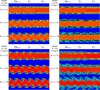 |
Fig. 10 Density rendering of the Kelvin-Helmholtz instability at t=2 (left column) and t=4 (right column) for an initial density contrast of ∆ρ = 2 (top panels) and ∆ρ = 8 (bottom panels) with the GDSPH method. The X and Y axes have a length of one. Here one can see a comparison in the development of the instability between the optimized kernel at a given Nsmooth and the popular Wendland C2 and C4 kernels. We observed a clear improvement in the optimized kernel, reproducing a similar behavior of the C4 kernel at double the neighbor count (Nsmooth). For the high density contrast ∆ρ = 8, there are only minor differences between the different kernels at Nsmooth = 128. These can be compared to the higher resolution cases given in Appendix A. |
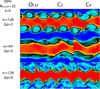 |
Fig. 11 Density rendering of the Kelvin-Helmholtz instability at t = 4 for Nsmooth = 32 with the ISPH method. The X and Y axes have a length of one. Here one can see a comparison in the development of the instability between the optimized kernel (OI, 32) and the popular Wendland C2 and C4 kernels. We have selected three cases where discernible differences can be seen (nx = 128, ∆ρ = 2; nx = 64, ∆ρ = 2; nx = 128, ∆ρ = 8). For the ∆ρ = 2 cases we observed that the C2 and C4 kernels exhibit more angular momentum errors (inherent to ISPH) compared to the OI,32 kernel, where the inner stream becomes significantly twisted, deviating from the high resolution and high Nsmooth results (see Appendix A). For the high density case nx = 128, ∆ρ = 8, we observed that C4 is unable to generate the same vortex structure in the upper plane of the stream and exhibit some asymmetry around the plane. |
4.4 Sod shock tube
Here we test the classic Sod shock tube (Sod 1978), where a fluid medium is initially divided into two separate regions with different pressures and densities. The initial conditions are ρleft = 1, Pleft = 1 for x < 0 and ρright = 0.25, Pright = 0.1795 for x > 0. We use an adiabatic equation of state with adiabatic index of Γ = 5/3. At the start of the simulation, we imagine removing a wall between the two regions creating a discontinuous state between the fluid’s generating a shockwave. The produced shockwave has three distinct regions, the right-moving shock front, the left-moving rarefaction wave, and the contact discontinuity. Here there are once again many ways to setup the initial distribution of particles. This case is particularly difficult due to the discontinuous density profile, as it is not possible to follow a discontinuous solution with the smooth density estimate. That is, even if two different density glasses or lattices are set up, the density should still be smoothed at the interface. One could either try one’s best to relax a glass following the discontinuous solution or smooth the initial shock by a tiny amount (proportional to the smoothing length). An argument against the complete discontinuous solution (in density) would be that it would rarely happen in a dynamic SPH simulation, as it would always be accompanied with some smoothing. Other quantities, such as velocities and thermal energy, of course occur discontinuously in simulations. We chose to smooth the discontinuity on the scale of the smoothing length. We used a thin periodic 3D box to approximate the 1D test, with Lx = 2.0 and Ly = Lz set to be roughly 16 particle spacings in the low density region. We used Lx = 2.0 due to using periodic boundary conditions such that the shock generated at the periodic boundary does not interact with the central shock. We used a resolution of around nx = 64 × 2 in the initial high density region (the factor of two is to account for the box extension). We used a constant α = 1 and β = 2 for the artificial viscosity.
As the velocity shows the biggest difference, we highlight the velocity structure between the different kernels in Fig. 13 for Nsmooth = 64. From this figure we can see that the optimized kernel’s exhibit less noise in the post-shock region compared to the Wendland C2 and C4 kernels for both GDSPH and ISPH. Other than that, there is not much difference between the kernels in this case.
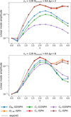 |
Fig. 12 Amplitude of the k = 2π mode over time for different smoothing kernels and density contrasts: ∆ρ = 2 (top) and ∆ρ = 8 (bottom). The ISPH method shows little difference between the different smoothing kernels, capturing a growth rate of roughly γ ∝ π in ∆ρ = 2 case and a slightly lower growth rate for ∆ρ = 8 (as expected). The GDSPH method of Nsmooth = 64 struggles to capture the same growth rate as the ISPH method, but we observed that the optimized kernel improves the growth rate of the KH mode for both ∆ρ = 2 and ∆ρ = 8. |
 |
Fig. 13 Velocity structure of the Sod-shocktube test at t = 0.2 performed at nx = 64 and Nsmooth = 64. The thin black line shows the exact solution. One can see that the optimized kernel exhibit less noise in the post-shock region compared to the C2 and C4 kernel. |
4.5 Evrard collapse
The Evrard collapse test (Evrard 1988; Steinmetz & Mueller 1993; Wadsley et al. 2017; Mandal et al. 2023), simulates the collapse of adiabatic gas, which include a high Mach shock and a cold pre-shock infall. The density is defined as
 (55)
(55)
where the initial cloud radius is R = 1 and the initial cloud mass is M = 1. The internal energy is u = 0.05GM/R and we use an adiabatic index of γ = 5/3. We setup the initial density using our IC generator, using roughly 28 000 particles. As this is an open boundary IC, we need to assume an initial low density medium for the IC generator to fit against. This is because the IC generator uses only the SPH forces to fit the density profile, this requires a periodic boundary and density to be defined everywhere. After the IC generator has fitted the density profile, we remove all particles beyond R = 1 and ensure that particle mass sum up to M = 1.
The biggest difference in the Evrard collapse (at t = 0.08) between the two methods GDSPH and ISPH and the different kernels can be seen in the noise level, similar to the Sod shocktube test. In Fig. 14 we can see the velocity structure of the two SPH methods and kernels. The noise level of C4 is slightly larger than the C2 and the optimized kernels. With C4 having a slightly sharper shock front than the other two.
4.6 Subsonic blob test
The blob test consist out of a high density spherical cloud at rest within a uniformly flowing low density medium. As the high density blob is accelerated by the surrounding medium, fluid instabilities such as Kelvin-Helmholtz and Rayleigh-Taylor instabilities disrupts the cloud and mixes it with the surrounding medium. The original blob test of Agertz et al. (2007), models a wind with a super sonic Mach number of M = 2.7. However, we have seen from the Sod shock tube and Evrard collapse tests, that the quality of the smoothing kernel does not have much effect on high Mach tests. Particle noise and kernel errors are more relevant for subsonic flows, and as such we decided to instead model a subsonic blob test with a Mach number of M = 0.5 to test the effect of the kernels on the mixing in the subsonic regime. The domain is periodic, with dimensions (10,10,40) in units of cloud radius. The cloud was put in pressure equilibrium and has a density ratio of Pρ = ρcloud/ρwind = 100. The wind velocity was set by the Mach number vwind = Mcs, and we defined the characteristic cloud crushing time to be  and ran the simulation for 10tcrush. In our analysis of the blob test, we defined the cloud mass to be Mcloud = M(ρ > ρcloud/3) and the intermediate temperature mass as in Braspenning et al. (2023); Sandnes et al. (2025):
 (56)
(56)
Here, mi is mass of the particle, Ti is the temperature of the particle, and Tmix is the geometric mean temperature:  .
.
From the top panel of Fig. 16, we can see that all models disrupts the cloud and reduces the high density mass in a few cloud crushing times (3-5 tcrush). However, it is clear from the rendering of the simulation at t = 5tcrush in Fig. 15 that the mixing of the gas with the surrounding medium differs between the different SPH methods and smoothing kernels. This can also be seen in the intermediate temperature mass evolution, where initially this mass increase is similar in all models, but the subsequent mixing of this mass with the warm medium evolves very differently. ISPH mixes the cloud more aggressively than GDSPH, where for ISPH at t = 5tcrush most of the intermediate temperature mass have mixed with the surrounding medium, while GDSPH have majority of the initial cloud mass in this intermediate temperature. The result of the intermediate temperature mass, is reminiscent of the KH mode amplitude growth dependency that we saw in Fig. 12.
 |
Fig. 14 Velocity structure of the Evrard collapse at t = 0.8 performed with 28000 particles and Nsmooth = 64. The thin black line shows the reference solution from a 1D PPM simulation with 8192 grid points (Mandal et al. 2023). One can see that the optimized kernel and the C2 kernel exhibit less noise in the post-shock region compared to the C4 kernel. |
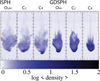 |
Fig. 15 Density rendering of the subsonic blob test (∆ρ = 100, M = 0.5 Rcloud = 0.1) at t = 5tcrush with a resolution of nx = 64 in the low density medium. The three left columns depict the cloud state with the ISPH method and the kernels (OI,64, C2, C4), and three right columns show the GDSPH method and the kernels (O64, C2, C4). The X axis has a length of one, and Y axis has a length of three. One can see that the ISPH method disrupts and mixes the cloud more aggressively than the GDSPH method. We also observed that we increase mixing with the optimized kernels compared to the C2 and C4 kernel in both the GDSPH and ISPH method. |
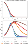 |
Fig. 16 Time evolution of the cloud mass ( |

5 Discussion
In this paper we have generated a set of new optimized kernels through the linear combination of other positive-definite kernels whose coefficients were optimized for the GDSPH method for the hydrostatic glass, the Gresho-Chan vortex, and for the ISPH method for the Gresho-Chan vortex. We find that the kernels optimized for the hydrostatic glass perform significantly worse for dynamical cases. We find that all kernels that had regular large oscillations in their Fourier transform performed worse for the Gresho-Chan vortex. The kernels produced by optimizing to the Gresho-Chan vortex all produce a quite steady decreasing Fourier transform with very slight oscillatory behavior and with a very similar functional form to that of the C2 kernel. However, compared to the C2 kernel, the majority of optimized kernels have a Fourier transform that decreases more rapidly with wave numbers (past k > 3π). We observed that in general, the Fourier transform decreases faster past k > 3π for the kernels optimized at a higher neighbor number, and it decreases faster before k < 3π for the kernels optimized at a lower neighbor number. Having a lower power at a high wave number seems to be important for higher neighbor numbers, while a lower power at low wave numbers is important for smaller neighbor numbers.
The new optimized kernels produce significant improvements for the GDSPH method, showing an improvement for the Gresho-Chan vortex (nx = 64 t = 1) L1,error of −20, −41, −31, and −17% relative to the L1,error of the C2 kernel for Nsmooth = 32,64,128,256, respectively. The optimized kernel for Nsmooth = 64 gives roughly the same L1,error as that of Nsmooth = 128 for the C2 kernel. At the later time, we observed that the O256 kernel performs better than O128 for all nx and even better than O64 at higher resolution (nx = 128,256), as O256 performs quite well even at t = 1 for both Nsmooth = 64 and Nsmooth = 128. One could use O256 for all Nsmooth > 64. The C4 kernel has the steepest improvement for Nsmooth = 256, remaining near linear with resolution, while O256 starts to flatten out beyond nx = 256. This is likely due to the fact that O256 reduces zero- and first-order errors a lot, while C4 reduces higher-order errors more than O256. For ISPH, we also observed improvements of the L1,error in the Greso-Chan vortex, which are −30, −21, −11, and −8% relative to the L1,error of the C2 kernel for Nsmooth = 32,64,128,256, respectively. This is visible mainly in a reduction of noise. At the later time, there is much less difference between the kernels at the higher Nsmooth = 128,256, while a significant improvement can still be seen for Nsmooth = 32, 64. The C2 kernel is in general the best-performing smoothing kernel from the non-optimized kernels for most Nsmooth. At later times, at t = 3, we observed that C4 performs better at Nsmooth = 64 for GDSPH, the reason for which is not fully clear, and Nsmooth = 256 for the ISPH method, where C4 is the best-performing kernel of all at t = 3, likely due to the leading orders being much lower and thus giving more importance to higher-order errors. The noise of Nsmooth = 256 for the ISPH method for C4 is still greater than the OI,256 kernel, as can be seen in Fig. 6. But the peak of the vortex is slightly higher with the C4 kernel. We can compare the convergence rate ( ) to Cabezón & García-Senz (2024), who used ISPH and mix Sinc kernels to provide a more accurate and stable kernel against pairing instability. Those authors show a convergence rate of p = 0.2 at Nsmooth = 60 to p = 1.03 at Nsmooth = 400 after t = 1. For ISPH/GDSPH(t = 3)[t = 1] and the optimized kernels, we show a convergence rate of (p = 0.5/p = 0.3)[p = 0.4/p = 0.3] at Nsmooth = 32, /(p = 0.6/p = 0.5)[p = 0.5/p = 0.5] at Nsmooth = 64, (p = 0.9/p = 0.7)[p = 0.8/p = 0.7] at Nsmooth = 128 to (p = 1.1/p = 0.9)[p = 1.0/p = 0.9] at Nsmooth = 256 after (t = 3)[t = 1]. In Wadsley et al. (2017), with modern artificial viscosity switches, they found a convergence rate of p = 0.8 for Nsmooth = 200 with the C4 kernel at t = 3. The moving mesh code AREPO in Springel (2010) yields a convergence rate of p = 1.4. Note that comparison to other modern SPH codes is slightly unfair, as we used a classic artificial viscosity scheme with constant α and β values, where we have chosen a low α value that gives a good result for the Gresho-Chan vortex.
For the Kelvin-Helmholtz instability, the biggest improvement could be seen for the GDSPH method, where the new optimized kernels captured similar results to that of the C4 kernel at double Nsmooth (both at ∆ρ = 2 and ∆ρ = 8 density contrast). For the ISPH method, the main improvement could be seen in angular momentum conservation of the low Nsmooth runs, where OI,32 performs better than C2 and C4. For the Sod-shocktube and Evrard collapse test, the main improvement of the optimized kernels could be seen as a reduction of the noise in the post-shock region.
In conclusion, we find that the linear-combination of kernels generates optimized kernels that significantly improve results, particularly in the low Nsmooth regime. This can give a result similar to doubling the Nsmooth of previous smoothing kernels (C2, C4) without any additional computational cost.
For ISPH, the results of the linear fluid behavior is only weakly dependent on the smoothing kernel and neighbor number (as seen in the Gresho-Chan vortex and the KH instability). We could see that the particle noise, angular momentum errors, and the mixing of the subsonic blob test improved with the new optimized kernels. For GDSPH, we observed an overall improvement with the optimized kernels for all test cases. From these tests we observed that ISPH give a significant improvement in convergence and behavior for subsonic flows compared to GDSPH. Results from the high Mach tests such as the Sod shocktube and Evrard collapse are much more insensitive to the SPH method and smoothing kernel used. For GDSPH, we recommend using O32 for Nsmooth <= 32, O64 for Nsmooth <= 96, and O256 for higher values of Nsmooth. For ISPH, we recommend using OI,32 for Nsmooth <= 32, OI,64 for Nsmooth <= 96, and OI,256 for higher values of Nsmooth.
We have introduced a new IC generator to generate glass distributions of arbitrary density profiles in SPH. We have also introduced self-bias corrections to the kernel, that have been adjusted to the glass distribution instead of the lattice distribution of earlier work. This ensures more accurate density interpolation for the glass distribution of positive-definite kernels used in this paper.
This work shows that targeted kernel optimization can enhance SPH convergence beyond what is achievable with the standard compact kernels commonly used. It also demonstrates that the most effective kernel for a given problem depends on the specific SPH formulation used. These findings motivate future exploration of new optimization strategies and further improvements to both the smoothing kernels and the SPH method as a whole.
Data availability
The initial condition generator, optimized kernels, and test cases used in this work are publicly available at: https://github.com/robertwissing/testsuite.
Acknowledgements
We acknowledge support from the European High Performance Comput- ing Joint Undertaking (EuroHPC JU) and the Research Council of Norway through the funding of the SPACE Center of Excellence (grant agreement N0 101093441). Parts of the simulations were performed using the resources from the National Infrastructure for High Performance Computing and Data Storage in Norway, UNINETT Sigma2, allocated to Project NN9477K. We acknowledge the use of SPLASH (Price 2007) for the visualization of the results.
References
- Agertz, O., Moore, B., Stadel, J., et al. 2007, MNRAS, 380, 963 [NASA ADS] [CrossRef] [Google Scholar]
- Bonet, J. 1999, Comp. Methods Appl. Mech. Eng., 180, 97 [Google Scholar]
- Børve, S., Omang, M., & Trulsen, J. 2004, ApJS, 153, 447 [Google Scholar]
- Braspenning, J., Schaye, J., Borrow, J., & Schaller, M. 2023, MNRAS, 523, 1280 [Google Scholar]
- Brookshaw, L. 1985, PASA, 6, 207 [NASA ADS] [CrossRef] [Google Scholar]
- Buhmann, M. D. 1998, Proc. Edinburgh Math. Soc., 41, 33 [Google Scholar]
- Buhmann, M. D. 2003, Radial Basis Functions (Cambridge: Cambridge University Press) [Google Scholar]
- Cabezón, R. M., & García-Senz, D. 2024, MNRAS, 528, 3782 [Google Scholar]
- Cabezón, R. M., García-Senz, D., & Relaño, A. 2008, J. Comput. Phys., 227, 8523 [CrossRef] [Google Scholar]
- Cabezón, R. M., García-Senz, D., & Figueira, J. 2017, A&A, 606, A78 [NASA ADS] [CrossRef] [EDP Sciences] [Google Scholar]
- Chernih, A., & Hubbert, S. 2014, J. Approx. Theory, 177, 17 [Google Scholar]
- Cullen, L., & Dehnen, W. 2010, MNRAS, 408, 669 [NASA ADS] [CrossRef] [Google Scholar]
- Dehnen, W., & Aly, H. 2012, MNRAS, 425, 1068 [NASA ADS] [CrossRef] [Google Scholar]
- Diehl, S., Rockefeller, G., Fryer, C. L., Riethmiller, D., & Statler, T. S. 2015, PASA, 32, e048 [Google Scholar]
- Evrard, A. E. 1988, MNRAS, 235, 911 [Google Scholar]
- Frontiere, N., Raskin, C. D., & Owen, J. M. 2017, J. Comput. Phys., 332, 160 [NASA ADS] [CrossRef] [Google Scholar]
- García-Senz, D., Cabezón, R. M., & Escartín, J. A. 2012, A&A, 538, A9 [NASA ADS] [CrossRef] [EDP Sciences] [Google Scholar]
- García-Senz, D., Cabezón, R. M., Escartín, J. A., & Ebinger, K. 2014, A&A, 570, A14 [NASA ADS] [CrossRef] [EDP Sciences] [Google Scholar]
- Gresho, P. M., & Chan, S. T. 1990, Int. J. Numer. Methods Fluids, 11, 621 [Google Scholar]
- Lecoanet, D., McCourt, M., Quataert, E., et al. 2016, MNRAS, 455, 4274 [NASA ADS] [CrossRef] [Google Scholar]
- Lombardi, J. C., Sills, A., Rasio, F. A., & Shapiro, S. L. 1999, J. Comput. Phys., 152, 687 [Google Scholar]
- Mandal, A., Mukherjee, D., & Mignone, A. 2023, ApJS, 268, 40 [NASA ADS] [CrossRef] [Google Scholar]
- McNally, C. P., Lyra, W., & Passy, J.-C. 2012, ApJS, 201, 18 [NASA ADS] [CrossRef] [Google Scholar]
- Menon, H., Wesolowski, L., Zheng, G., et al. 2015, Comput. Astrophys. Cosmol., 2, 1 [NASA ADS] [CrossRef] [Google Scholar]
- Monaghan, J. J. 1988, Comp. Phys. Commun., 48, 89 [Google Scholar]
- Monaghan, J. J. 1992, ARA&A, 30, 543 [Google Scholar]
- Monaghan, J. J. 2005, Rep. Prog. Phys., 68, 1703 [NASA ADS] [CrossRef] [Google Scholar]
- Morris, J. P. 1996, PASA, 13, 97 [Google Scholar]
- Price, D. J. 2007, PASA, 24, 159 [Google Scholar]
- Price, D. J. 2012, J. Comput. Phys., 231, 759 [NASA ADS] [CrossRef] [Google Scholar]
- Price, D. J., & Monaghan, J. J. 2004, MNRAS, 348, 123 [Google Scholar]
- Price, D. J., Wurster, J., Tricco, T. S., et al. 2018, PASA, 35, e031 [Google Scholar]
- Read, J. I., & Hayfield, T. 2012, MNRAS, 422, 3037 [NASA ADS] [CrossRef] [Google Scholar]
- Rosswog, S. 2009, New A Rev., 53, 78 [Google Scholar]
- Rosswog, S. 2015, MNRAS, 448, 3628 [NASA ADS] [CrossRef] [Google Scholar]
- Rosswog, S. 2020, MNRAS, 498, 4230 [NASA ADS] [CrossRef] [Google Scholar]
- Rosswog, S. 2025, Comp. Model. Eng. Sci., 143, 1713 [Google Scholar]
- Sandnes, T. D., Eke, V. R., Kegerreis, J. A., et al. 2025, J. Comput. Phys., 532, 113907 [Google Scholar]
- Schaback, R. 2011, Adv. Comput. Math., 34, 67 [Google Scholar]
- Shen, S., Wadsley, J., & Stinson, G. 2010, MNRAS, 407, 1581 [NASA ADS] [CrossRef] [Google Scholar]
- Sod, G. A. 1978, J. Comput. Phys., 27, 1 [CrossRef] [MathSciNet] [Google Scholar]
- Springel, V. 2010, MNRAS, 401, 791 [Google Scholar]
- Steinmetz, M., & Mueller, E. 1993, A&A, 268, 391 [NASA ADS] [Google Scholar]
- Thomas, P. A., & Couchman, H. M. P. 1992, MNRAS, 257, 11 [Google Scholar]
- Tricco, T. S. 2019, MNRAS, 488, 5210 [NASA ADS] [CrossRef] [Google Scholar]
- Valdarnini, R. 2016, ApJ, 831, 103 [NASA ADS] [CrossRef] [Google Scholar]
- Wadsley, J. W., Keller, B. W., & Quinn, T. R. 2017, MNRAS, 471, 2357 [NASA ADS] [CrossRef] [Google Scholar]
- Wendland, H. 1995, Adv. Comput. Math., 4, 389 [CrossRef] [MathSciNet] [Google Scholar]
- Wu, Z. 1995, Adv. Comput. Math., 4, 283 [Google Scholar]
This is in regard to constant smoothing length or accounting for changes in smoothing length, h, through ∇h terms.
When equal flux enters through each surface area between particles (e.g., for constant pressure), a disparity in effective area on either side results in movement toward the side with a smaller effective area. This occurs because the sum of the effective areas between particles and their normals do not cancel out.
The gradient of the smoothing kernel gives the effective area between two particles.
The drawbacks of using a high number of neighbors is the additional computational cost and the increase in smoothing length (h), which can lead to excessive smoothing of sharp features in the flow.
One can take two glass boxes with different densities and put them next to each other; however, the interface in such a setup is not in a relaxed distribution. And if one wants to smooth the density contrast, this also becomes problematic.
One could even set n = 0, that is Pa = 1 and relax the distribution, this would disregard the density estimate and instead assume an exact value of the density. This could be used if one evolves the density from the continuity equation  for example, to minimize gradient errors.
Appendix A Differences between GDSPH and ISPH
In this appendix we include a resolution study between GDSPH and ISPH for the KH instability using the new optimized kernels for each respective Nsmooth, which can be seen in Fig. A.1 for ∆ρ = 2 and Fig. A.2 for ∆ρ = 8. From these figures it is clear that the result for ISPH is highly independent of Nsmooth, producing the same solution for Nsmooth = 32 and Nsmooth = 128. The GDSPH results are on the other hand, much more dependent on Nsmooth, and exhibit severe damping of the instability at Nsmooth = 32. At Nsmooth = 128, the GDSPH method produces similar structures to that of the ISPH method at ∆ρ = 2. For high density contrast ∆ρ = 8, we can see that high Nsmooth for the ISPH method generates more noise at the boundary layer at t = 2 compared to GDSPH in this case. We can also see that at later time, the high density structures are more dissipate in the ISPH method compared to the GDSPH method. We still see much more consistent behavior in the ISPH method compared to GDSPH method.
The high density contrast KH instability, is interesting as it is usually accompanied with strong surface tension effects in the Lagrangian formalism of SPH, due to high E0 and E1 errors at the discontinuous boundary. In GDSPH, these errors are reduced by doing a geometric density weighting in the gradient operator, reducing the errors at the density contrast. This sort of correction, deviates from the density estimate derivation of Lagrangian SPH and will thus introduce an entropy error. In GDSPH this is corrected for so that the method remains second-order accurate in entropy. ISPH removes the linear gradient error from it’s gradients, which effectively removes more of the "partition" force that exist in SPH and only have E0 error forces to remain ordered. This sort of correction also introduces entropy errors, which would potentially be first order in this case. In Fig. A.3, we show how one of the KH swirls develops when not using diffusion versus using diffusion for both the GDSPH and ISPH methods. Significant amounts of entropy bubbles can be seen in the ISPH version without diffusion, and a few can be seen in GDSPH. Adding thermal diffusion (Shen et al. 2010) allows for local mixing between the cold and hot phases, and we can see that we get good behavior in both ISPH and GDSPH. Slight numerical surface tension effects can be seen for GDSPH, while none can be seen for ISPH.
Appendix B Kernel self-bias correction coefficients
In this section we present the self-correction bias coefficients present in
 (B.1)
(B.1)
 (B.2)
(B.2)
where Nmin,i ∈ {16,24,32,48,64,96,128,256,512). The ci coefficients can be found in Table B.1 for all kernels.
Appendix C Kernel tables
The linear-combination of kernels after optimization are fitted are fitted to a polynomial in the form
 (C.1)
(C.1)
 (C.2)
(C.2)
The polynomial coefficients for all the optimized kernels are given in C.1 and C.2.
Appendix D Code implementation
A simple code snippet of the kernel function is included for clarification and for easier implementation, for both GDSPH and ISPH.
 |
Fig. A.1 Density rendering of the Kelvin-Helmholtz instability (∆ρ = 2) at t = 2 (three left columns) and t = 4 (three right columns) for varying resolution (nx = 64,128,256), Nsmooth = 32,64,128, and method (GDSPH upper three rows and ISPH bottom three rows). The X and Y axis have a length of 1a. These simulations were all run with the optimized kernel for each ONsmooth GDSPH and OI,Nsmooth for ISPH. We can see that ISPH manages to generate the same vortex structure, regardless of the number of neighbors if the resolution is high enough, while GDSPH struggles with lower number of neighbors even at the highest resolution. |
 |
Fig. A.2 Density rendering of the Kelvin-Helmholtz instability (∆ρ = 8) at t = 2 (three left columns) and t = 4 (three right columns) for varying resolution (nx = 64,128,256), Nsmooth = 32,64,128, and method (GDSPH upper three rows and ISPH bottom three rows). The X and Y axis have a length of 1. These simulations were all run with the optimized kernel for each ONsmooth GDSPH and OI,Nsmooth for ISPH. Similar as the low density version of Fig. A.1, we can see that ISPH captures instability well regardless of neighbor number. We can see additional diffusion from the ISPH runs compared to the GDSPH runs, even with the highest resolution. There also seem to be additional noise in the small-scale density structures as we increase the number of neighbors for ISPH. Potentially related to the issue found in Fig. A.3 |
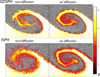 |
Fig. A.3 Particle density rendering of Kelvin-Helmholtz instability swirl at t = 2 for ∆ρ = 8. The figures shows the different behavior of not using diffusion versus using diffusion for the GDSPH and ISPH methods. A significant number of entropy clumps can be seen being generated in the low density medium for ISPH, as the removal of linear gradient together with sharp boundaries causes chaotic noise at the boundary. Lagrangian SPH formalisms that are derived directly from the density estimate, provide full spatial conservation of entropy. However, deviation from the Lagrangian formalism, while still using the traditional density estimate means that we will introduce entropy errors in our solution. GDSPH corrects for firstorder errors in entropy making it second-order in entropy. ISPH removes linear-gradient errors and will thus only be first-order accurate with entropy. The issue might be further aggravated by the use of average gradient kernels within ISPH. Adding thermal diffusion allows for local mixing between the cold and hot phase, and we can see that we get good behavior in both ISPH and GDSPH. Slight numerical surface tension effect can be seen for GDSPH, while none can be seen for ISPH. |
Polynomial coefficients for all the optimized kernels based on the hydrostatic glass test case.
Polynomial coefficients for all the optimized kernels based on the Gresho-Chan test case.
Contribution of each kernel in the linear combination used to optimize all kernels for the Gresho-Chan test case.


All Tables
Polynomial coefficients for all the optimized kernels based on the hydrostatic glass test case.
Polynomial coefficients for all the optimized kernels based on the Gresho-Chan test case.
Contribution of each kernel in the linear combination used to optimize all kernels for the Gresho-Chan test case.
All Figures
|
Fig. 1 Relaxed glass IC generated by the IC generator outlined in Sect. 3.2. Here we model the IC of the Kelvin Helmholtz instability (Sect. 4.3), with a density contrast of ∆ρ = 8. Top : particle distribution within a thin slice of thickness ∆ z = 0.015. Bottom : density profile in the y direction. The red line depicts the analytical density profile and the black dots the density of the particles. The glass generated density profile is in excellent agreement with the analytical solution. |
| In the text | |
|
Fig. 2 Top : optimized kernel functions for a glass distribution (Sect. 3.4.1) together with the missing Wendland kernels (CM04, CM05), the Buhmann kernel (BUH), and the Wu kernel (WU2). Middle : corresponding derivative of these kernel function. Bottom: fourier transform of these kernels, scaled by k/10. The optimized kernels are quite similar, with some small variations being seen in the Fourier transform. The Oglass,32 kernel deviates the most from the other kernel, with less deep troughs in the Fourier transform. These kernel’s generate excellent glass distributions but degrade significantly in dynamical simulations. |
| In the text | |
|
Fig. 3 Top : optimized kernel functions for the Gresho-Chan vortex (Sect. 3.4.2), for both GDSPH and ISPH together with the popular Wendland kernels (C2, C4). Middle : corresponding derivative of these kernel function. Bottom : fourier transform of these kernels, scaled by k/10. The optimized kernel exhibit a clear trend in it’s Fourier transform, where the kernels optimized for higher Nsmooth emphasizes lower power beyond k > 3π. The general form of the optimized kernel is quite similar to the Wendland C2 kernel. In general GDSPH produces lower power than ISPH in the high wave number regime for a given Nsmooth. The OI,32 kernel is the only optimized kernel that exhibits a negative Fourier transform at low wavenumbers. Among the other optimized kernels, only O256 has a negative Fourier transform, but this occurs at higher wavenumbers and remains stable to pairing instability up to at least Nsmooth < 500. |
| In the text | |
|
Fig. 4 Relative increase or decrease of the δρerr (top), E0 (middle), and E1 (bottom) of the hydrostatic glass when relaxed for different kernels in respect to the corresponding error of the C2 kernel. The simulations here were performed with only the GDSPH method. The terms N32, N64, N128, and N256 refer to the number of neighbors: Nsmooth = 32,64,128,256, respectively. The δρerr, E0 and E1 of the C2 kernel for each Nsmooth is δρerr = 5.539 × 10−3,3.747 × 10−3,1.243 × 10−3,5.860 × 10−4, E0 = 2.763 × 10−3,2.024 × 10−3, 6.797 × 10−4,4.253 × 10−4, and E1 = 2.210 × 10−2,1.484 × 10−2,2.557 × 10−3,8.305 × 10−4. The optimized kernels can in general be seen to drastically reduce the E1 error relative to the C2 kernel. For the glass optimized kernel’s we can also see a general decrease in both δρ and E0 for their given Nsmooth. |
| In the text | |
|
Fig. 5 Relative increase or decrease of the L1,error of the Gresho-chan vortex at t = 1 and nx = 64 for different kernels in respect to the L1,error of the C2 kernel. The terms N32, N64, N128, and N256 refer to the number of neighbors: Nsmooth = 32,64,128,256. Left : simulations done with the GDSPH method. Right : simulations done with the ISPH method. The L1,error of the C2 kernel for each Nsmooth is L1,error = 1.49375 × 10⁻¹, 9.57342 × 10⁻², 4.70888 × 10⁻², 2.99816 × 10⁻² for GDSPH and L1,error = 9.34635 × 10⁻², 4.66192 × 10⁻², 2.64744 × 10⁻², 2.22268 × 10⁻² for ISPH. An improvement for the optimized kernel at a given Nsmooth across all Nsmooth can be seen for both methods, where the biggest improvements are for the N64 and N128 for GDSPH and N32 and N64 for ISPH. Of the non-optimized kernels, we observed that the C2 kernel performs best, except for Nsmooth = 32 (GDSPH), Nsmooth = 32,64 (ISPH), where CM05 performs better and C4 performs slightly better at Nsmooth = 256 (ISPH). |
| In the text | |
|
Fig. 6 Azimuthal velocity in the radial direction of the Gresho-Chan vortex at t = 3. Here the resolution is nx = 64 and simulation was performed with GDSPH (left three columns) and ISPH (right three columns). We compare the optimized kernel at a given Nsmooth to the popular Wendland C2 and C4 kernels, and vary the number of neighbors in each row (Nsmooth = 32,64,128,256), referred here to N32, N64, N128, N256. The solid black line show the analytical solution and the black dots show the results from the simulation. The X axis (cylindrical radius) extends from 0.0 to 0.7, and the vertical extent from the top to the bottom of the analytical solution is 1. We can see a significant improvement in the optimized kernels for the GDSPH method for Nsmooth = 32,64,128, where the vortex structure becomes more pronounced. Overall less noise can be seen for all Nsmooth. The ISPH method captures the overall vortex structure well for all Nsmooth, due to exact linear gradients. But we can see significant improvement in the noise level of the optimized kernels, compared to the C2 and C4 kernels. |
| In the text | |
|
Fig. 7 Convergence study of the Gresho-Chan vortex with the GDSPH method for Nsmooth = 32,64,128,256. Here we plot the L1,error over resolution elements in the x direction (nx) at t = 3. Significant improvements can be seen for all optimized kernels compared to the Wendland C2 and C4 kernels. The kernels were optimized in respect to an earlier time t = 1 and we can see that O256 have an improved result over O128 for Nsmooth = 128 at this later time, even beating out O64 for Nsmooth = 64 at higher resolution (nx > 128). The C4 kernel exhibits slightly better convergence slope at high Nsmooth and nx > 128, likely due to it’s higher order properties (fewer O(h2) errors). |
| In the text | |
|
Fig. 8 Convergence study of the Gresho-Chan vortex with the ISPH method for Nsmooth = 32,64,128,256. Here we plot the L1,error over the resolution elements in the x direction (nx) at t = 3. Significant improvements can be seen for the optimized kernels at Nsmooth = 32,64 compared to the Wendland C2 and C4 kernels. While at higher Nsmooth, there is much less difference between all the kernels. The kernels were optimized in respect to an earlier time, t = 1, and we observed that C4 performs better at this later time for Nsmooth = 256 than all the optimized kernels at all resolutions. This is surprising, as E0 errors of the optimized kernels are much lower than the C4 kernel (see Fig. 9), which might indicate that long-term behavior at this Nsmooth is heavily determined by the higher order errors (O(h2)). |
| In the text | |
|
Fig. 9 Convergence study of the Gresho-Chan vortex with the ISPH method for Nsmooth = 256. Here we plot the E0 error versus the number of resolution elements in the x direction (nx) at t = 3. Much lower zeroth order errors for the optimized kernel and C2 kernel can be seen compared to the higher order C4 kernel. Note here that even though being zeroth order (dependent on local particle order), the error still decreases with increasing resolution ( |
| In the text | |
|
Fig. 10 Density rendering of the Kelvin-Helmholtz instability at t=2 (left column) and t=4 (right column) for an initial density contrast of ∆ρ = 2 (top panels) and ∆ρ = 8 (bottom panels) with the GDSPH method. The X and Y axes have a length of one. Here one can see a comparison in the development of the instability between the optimized kernel at a given Nsmooth and the popular Wendland C2 and C4 kernels. We observed a clear improvement in the optimized kernel, reproducing a similar behavior of the C4 kernel at double the neighbor count (Nsmooth). For the high density contrast ∆ρ = 8, there are only minor differences between the different kernels at Nsmooth = 128. These can be compared to the higher resolution cases given in Appendix A. |
| In the text | |
|
Fig. 11 Density rendering of the Kelvin-Helmholtz instability at t = 4 for Nsmooth = 32 with the ISPH method. The X and Y axes have a length of one. Here one can see a comparison in the development of the instability between the optimized kernel (OI, 32) and the popular Wendland C2 and C4 kernels. We have selected three cases where discernible differences can be seen (nx = 128, ∆ρ = 2; nx = 64, ∆ρ = 2; nx = 128, ∆ρ = 8). For the ∆ρ = 2 cases we observed that the C2 and C4 kernels exhibit more angular momentum errors (inherent to ISPH) compared to the OI,32 kernel, where the inner stream becomes significantly twisted, deviating from the high resolution and high Nsmooth results (see Appendix A). For the high density case nx = 128, ∆ρ = 8, we observed that C4 is unable to generate the same vortex structure in the upper plane of the stream and exhibit some asymmetry around the plane. |
| In the text | |
|
Fig. 12 Amplitude of the k = 2π mode over time for different smoothing kernels and density contrasts: ∆ρ = 2 (top) and ∆ρ = 8 (bottom). The ISPH method shows little difference between the different smoothing kernels, capturing a growth rate of roughly γ ∝ π in ∆ρ = 2 case and a slightly lower growth rate for ∆ρ = 8 (as expected). The GDSPH method of Nsmooth = 64 struggles to capture the same growth rate as the ISPH method, but we observed that the optimized kernel improves the growth rate of the KH mode for both ∆ρ = 2 and ∆ρ = 8. |
| In the text | |
|
Fig. 13 Velocity structure of the Sod-shocktube test at t = 0.2 performed at nx = 64 and Nsmooth = 64. The thin black line shows the exact solution. One can see that the optimized kernel exhibit less noise in the post-shock region compared to the C2 and C4 kernel. |
| In the text | |
|
Fig. 14 Velocity structure of the Evrard collapse at t = 0.8 performed with 28000 particles and Nsmooth = 64. The thin black line shows the reference solution from a 1D PPM simulation with 8192 grid points (Mandal et al. 2023). One can see that the optimized kernel and the C2 kernel exhibit less noise in the post-shock region compared to the C4 kernel. |
| In the text | |
|
Fig. 15 Density rendering of the subsonic blob test (∆ρ = 100, M = 0.5 Rcloud = 0.1) at t = 5tcrush with a resolution of nx = 64 in the low density medium. The three left columns depict the cloud state with the ISPH method and the kernels (OI,64, C2, C4), and three right columns show the GDSPH method and the kernels (O64, C2, C4). The X axis has a length of one, and Y axis has a length of three. One can see that the ISPH method disrupts and mixes the cloud more aggressively than the GDSPH method. We also observed that we increase mixing with the optimized kernels compared to the C2 and C4 kernel in both the GDSPH and ISPH method. |
| In the text | |
|
Fig. 16 Time evolution of the cloud mass ( |
| In the text | |
|
Fig. A.1 Density rendering of the Kelvin-Helmholtz instability (∆ρ = 2) at t = 2 (three left columns) and t = 4 (three right columns) for varying resolution (nx = 64,128,256), Nsmooth = 32,64,128, and method (GDSPH upper three rows and ISPH bottom three rows). The X and Y axis have a length of 1a. These simulations were all run with the optimized kernel for each ONsmooth GDSPH and OI,Nsmooth for ISPH. We can see that ISPH manages to generate the same vortex structure, regardless of the number of neighbors if the resolution is high enough, while GDSPH struggles with lower number of neighbors even at the highest resolution. |
| In the text | |
|
Fig. A.2 Density rendering of the Kelvin-Helmholtz instability (∆ρ = 8) at t = 2 (three left columns) and t = 4 (three right columns) for varying resolution (nx = 64,128,256), Nsmooth = 32,64,128, and method (GDSPH upper three rows and ISPH bottom three rows). The X and Y axis have a length of 1. These simulations were all run with the optimized kernel for each ONsmooth GDSPH and OI,Nsmooth for ISPH. Similar as the low density version of Fig. A.1, we can see that ISPH captures instability well regardless of neighbor number. We can see additional diffusion from the ISPH runs compared to the GDSPH runs, even with the highest resolution. There also seem to be additional noise in the small-scale density structures as we increase the number of neighbors for ISPH. Potentially related to the issue found in Fig. A.3 |
| In the text | |
|
Fig. A.3 Particle density rendering of Kelvin-Helmholtz instability swirl at t = 2 for ∆ρ = 8. The figures shows the different behavior of not using diffusion versus using diffusion for the GDSPH and ISPH methods. A significant number of entropy clumps can be seen being generated in the low density medium for ISPH, as the removal of linear gradient together with sharp boundaries causes chaotic noise at the boundary. Lagrangian SPH formalisms that are derived directly from the density estimate, provide full spatial conservation of entropy. However, deviation from the Lagrangian formalism, while still using the traditional density estimate means that we will introduce entropy errors in our solution. GDSPH corrects for firstorder errors in entropy making it second-order in entropy. ISPH removes linear-gradient errors and will thus only be first-order accurate with entropy. The issue might be further aggravated by the use of average gradient kernels within ISPH. Adding thermal diffusion allows for local mixing between the cold and hot phase, and we can see that we get good behavior in both ISPH and GDSPH. Slight numerical surface tension effect can be seen for GDSPH, while none can be seen for ISPH. |
| In the text | |
Current usage metrics show cumulative count of Article Views (full-text article views including HTML views, PDF and ePub downloads, according to the available data) and Abstracts Views on Vision4Press platform.
Data correspond to usage on the plateform after 2015. The current usage metrics is available 48-96 hours after online publication and is updated daily on week days.
Initial download of the metrics may take a while.