| Issue |
A&A
Volume 706, February 2026
|
|
|---|---|---|
| Article Number | A249 | |
| Number of page(s) | 27 | |
| Section | Stellar structure and evolution | |
| DOI | https://doi.org/10.1051/0004-6361/202557113 | |
| Published online | 13 February 2026 | |
Analysis of mass-transferring binary candidates in the Milky Way
1
Departament de Física Quà ntica i Astrofísica (FQA), Universitat de Barcelona (UB), c. Martí i Franquès 1 08028 Barcelona, Spain
2
Institut de Ciències del Cosmos (ICCUB), Universitat de Barcelona (UB), c. Martí i Franquès 1 08028 Barcelona, Spain
3
Institut d’Estudis Espacials de Catalunya (IEEC), Edifici RDIT, Campus UPC 08860 Castelldefels (Barcelona), Spain
4
DTU Space, Technical University of Denmark, Elektrovej 327 2800 Kgs. Lyngby, Denmark
5
Royal Observatory of Belgium, Avenue Circulaire Ringlaan 3 1180 Brussels, Belgium
6
University of Liège, Allée du 6 Août 19c (B5C) 4000 Sart Tilman Liège, Belgium
★ Corresponding author: This email address is being protected from spambots. You need JavaScript enabled to view it.
Received:
5
September
2025
Accepted:
26
November
2025
Abstract
Mass transfer between stars in binary systems profoundly impacts their evolution, yet many aspects of this process–especially the stability, mass loss, and eventual fate of such systems–remain poorly understood. One promising avenue to constrain these processes is through the identification and characterisation of systems undergoing active mass transfer. Inspired by the slow brightening preceding stellar merger transients, we worked on a method to identify Galactic mass-transferring binaries in which the donor is a Hertzsprung gap (HG) star. We constructed an initial sample of HG stars using the Gaia Early Data Release 3 contribution Starhorse catalogue, and we identified candidate mass-transferring systems by selecting sources that exhibit Balmer emission features (as seen in the low-resolution Gaia XP spectra), mid-infrared excess (from WISE photometry), and photometric variability (inferred from the error in the GaiaG-band magnitude). This multi-criteria selection yielded a sample of 67 candidates, which we further analysed using complementary photometric and spectroscopic data, as well as information from cross-matched archival catalogues. Among our candidates, we identified at least nine eclipsing binaries and some sources that are potential binaries as well. Three sources in our sample are strong candidates for mass-transferring binaries with a yellow component, and three more are binaries with a Be star. Notably, three sources in our sample are strong candidates for hosting a compact companion, based on their ultraviolet or X-ray signatures. The main sources of contamination in our search are hot but highly reddened stars–primarily Oe and Be stars–as well as regular pulsating stars such as δ Scuti and Cepheid variables. As an additional outcome of this work, we present a refined new catalogue of 308 HG stars, selected using improved extinction corrections and stricter emission-line criteria. This enhanced sample is expected to contain a significantly higher fraction of scientifically valuable mass-transferring binaries.
Key words: binaries: close / binaries: eclipsing / stars: emission-line / Be / Hertzsprung-Russell and C-M diagrams
© The Authors 2026
 Open Access article, published by EDP Sciences, under the terms of the Creative Commons Attribution License (https://creativecommons.org/licenses/by/4.0), which permits unrestricted use, distribution, and reproduction in any medium, provided the original work is properly cited.
This article is published in open access under the Subscribe to Open model. This email address is being protected from spambots. You need JavaScript enabled to view it. to support open access publication.
1. Introduction
A large fraction of stars in the observable Universe are found in binary or multiple systems, with the likelihood of multiplicity increasing with stellar mass (Sana et al. 2012; de Mink et al. 2014; Moe & Di Stefano 2017). The evolution of most of these systems is significantly influenced by mass transfer between the components. How mass transfer unfolds and its eventual outcome strongly depend on the initial configuration of the binary and the nature of the mass transfer process. Broadly, two scenarios are considered: stable mass transfer, in which the mass exchange occurs without disrupting the system, and unstable mass transfer, where the accreting star is unable to absorb all the material from the donor, resulting in the formation of a common envelope that engulfs both stars (Kuiper 1941; Paczynski 1976).
Mass transfer is an accepted explanation for the creation of many astrophysical phenomena, such as the Algol-type binaries (Crawford 1955), the evolution of closely orbiting stellar binaries into X-ray binaries (Verbunt 1993), cataclysmic variable stars (Kraft 1964), supernovae (Wang & Han 2012; Yoon et al. 2010), accretion-induced collapse (Ivanova & Taam 2004), and gravitational wave sources (Schneider et al. 2001), among others. However, the details of mass transfer and the possible mass and angular momentum loss of the process, as well as the fate of the evolving stars, are not well established and modelled yet.
In recent years, the study of mass transfer has gained renewed attention due to its fundamental link to the formation of compact binaries and, ultimately, gravitational wave sources. To constrain these processes, detailed studies of systems currently undergoing mass exchange are crucial. These efforts span a wide range of approaches: observational analyses of interacting systems such as TZ Dra (Kahraman Aliçavuş et al. 2022), AU Monocerotis (Armeni & Shore 2022), and the contact binary V2840 Cygni (Pothuneni et al. 2023); modelling well-studied binaries such as β Lyrae A (Mourard et al. 2018; Brož et al. 2021); and theoretical work aimed at understanding the underlying physics of mass transfer and common envelope evolution (Cehula & Pejcha 2023; Podsiadlowski 2001; Ivanova et al. 2001; Marchant et al. 2021; Röpke & De Marco 2023).
The outcome of unstable mass transfer has recently been linked to a class of optical transients known as luminous red novae (LRNe), whose peak luminosities lie between those of novae and supernovae (Munari et al. 2002; Soker & Tylenda 2003; Tylenda et al. 2011; Pejcha 2014; Pejcha et al. 2016). These transients are generally interpreted as the observational signatures of stellar coalescence events, providing rare but direct evidence of binary interaction and merger processes.
Over the last two decades, LRNe have been studied both in our Galaxy and in nearby galaxies. Despite the proximity, the only five confirmed and studied stellar mergers in the Milky Way (MW) include V4332 Sagittarii (discovered in 1994; Martini et al. 1999), V838 Monocerotis (2002; Munari et al. 2002; Bond et al. 2003), OGLE-2002-BLG-360 (2002; Tylenda et al. 2013), CK Vul (1670; Kato 2003), and, most notably, V1309 Scorpii (2008, Mason et al. 2010), whose pre-outburst photometry captured the final inspiral of a contact binary system (Tylenda et al. 2011). Additionally, about two dozen extra-galactic LRNe were found (see Pastorello & Fraser 2019, Blagorodnova et al. 2021, Reguitti et al. 2026, and references therein). These events share a number of defining characteristics: a rapid rise and redward evolution in colour, usually a double-peaked light curve followed by a plateau, and the presence of strong and narrow emission lines for hydrogen and low-ionisation elements.
Archival data taken prior to the outburst have shown that most confirmed LRN progenitors are predominantly yellow giants (YGs) or yellow supergiants (YSGs) with spectral types G, F, or, to a lesser extent, A (Blagorodnova et al. 2017; MacLeod et al. 2017; Blagorodnova et al. 2021; Cai et al. 2022; Pastorello et al. 2023). These stars are evolving off the main sequence (MS) and crossing the Hertzsprung gap (HG) on their way to the red giant branch (RGB). This phase is characterised by a rapid increase in the stellar radius of the evolving star. Given the presence of a nearby companion, the donor can overfill its Roche lobe and initiate unstable mass transfer, finally resulting in a stellar merger and a transient. In the few cases where pre-outburst data exist, the progenitor shows a gradual brightening lasting years, interpreted as mass loss and the formation of an extended pseudo-photosphere before coalescence. Despite these key discoveries, LRN progenitors remain largely unexplored (Pastorello & Fraser 2019).
Guided by the location of known LRN progenitors on the Hertzsprung-Russell (HR) diagram, a recent study presented a method for identifying Galactic LRN candidates likely to outburst within the next 1–10 years (Addison et al. 2022). The selection of candidates was based on the position in the HR diagram and the variability of the sources. The study first identified a set of stars falling in a low stellar density area between the MS and the RGB from the Gaia Data Release 2 (DR2; Gaia Collaboration 2016, 2018) and Gaia Early Data Release 3 (EDR3; Gaia Collaboration 2021), and explored their variability in different time-domain surveys to select slowly brightening sources. From an initial set of approximately 107 initial sources, 21 LRN precursor candidates were selected. Most of them shared similar characteristics: the presence of Hα and (sometimes) Hβ emission lines together with the existence of an infrared (IR) excess. One of the limitations of that study was the lack of reliable estimates for Galactic extinction in Gaia DR2 and EDR3, implying that the true colours of the sources were rather uncertain.
The release of extinction estimates in Gaia Data Release 3 (DR3; Gaia Collaboration 2023) and Gaia-related catalogues, such as Starhorse (Anders et al. 2022), opened the possibility to revise the previous work with more accurate colours and astrophysical parameters. In this paper, we make use of these catalogues to present a selection and characterisation of HG stars in the Milky Way (MW) with characteristics compatible with known LRN precursors and mass-transferring systems. We first make a selection of candidates, followed by an analysis using archival and new follow-up data to find binary systems during the unstable mass transfer phase, which could become LRNe in the near future. In addition, we aim to characterise the variability of stars in the HG to understand what other systems can mimic the behaviour expected for LRN precursor systems. Finding unstable mass-transferring binaries will be of great interest to the theoretical and observational communities studying the stability of mass transfer and its impact on the final fate of binary stars.
2. Sample selection
Our initial selection strategy made use of Gaia DR3 data and the Gaia EDR3 StarHorse catalogue, in combination with mid-IR photometry from the AllWISE catalogue (Cutri et al. 2021). The selection steps are listed below:
-
To select HG stars, we used StarHorse, which (among other astrophysical parameters) contains absolute magnitudes in the G band and de-reddened BP − RP colours. Based on MESA Isochrones & Stellar Tracks (Paxton et al. 2011; Dotter 2016), we selected sources with absolute magnitudes MG < 1.5 mag, to avoid contamination from lower MS stars with masses ≲2 M⊙, and we also applied two cuts to select stars between the MS and the RGB. Finally, we removed a portion of the colour-magnitude diagram populated by Red Clump stars, known red giants in the horizontal branch. In Fig. 1a our initial parameter space is shown.
-
To select sources with emission in Hα or Hβ, we used the method developed by Weiler et al. (2023) to derive the equivalent width (EW) of the lines using the internally calibrated Gaia XP spectra (Carrasco et al. 2021; De Angeli et al. 2023) (see Fig. 1b, which shows the XP spectrum of one of our sources alongside the corresponding follow-up spectrum). We first tested this method with the candidates in Addison et al. (2022). The sources with Hα emission had positive EW values (as expected), but some of these sources showed high errors and low statistical significance in our EW calculation, even though they had clear emission in both the Gaia XP spectrum and a higher resolution follow-up spectrum. Therefore, we selected sources with a positive Hα or Hβ EW, without taking into account the EW error or the statistical significance.
-
To select sources with mid-IR excess associated with warm dust emission (likely from a disk), we used the AllWISE catalogue. We applied the following recommended quality cuts1: cc_flags = 0000, making sure the sources are unaffected by known artefacts; ext_flag = 0, indicating that the sources’ shape is consistent with a point-source, and ph_qual =A, B or C, selecting sources with a flux signal-to-noise ratio better than 2. We selected sources with W1(3.4 μm)−W4(22 μm) > 1, based on the distribution of sources in the W1(3.4 μm)−W4(22 μm) vs W1(3.4 μm)−W2(4.6 μm) colour-colour diagram (see Fig. 1c).
-
As the photometry listed in the main Gaia DR3 catalogue is a weighted average of the individual measurements taken in different transits (Riello et al. 2021), one expects that variable stars have higher photometric uncertainties (as seen in Andrew et al. 2021 or Maíz Apellániz et al. 2023). Thus, we placed our initial HG sample in the log10(Gerr) vs G plane (see Fig. 1d) and selected sources above the 90th percentile.
-
As a final step, we removed the sources with a known type in the SIMBAD (Wenger et al. 2000) database, for which the variability was associated with pulsations rather than binarity (such as RR Lyrae or Cepheids).
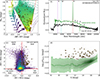 |
Fig. 1. Initial selection of our sample of mass-transferring candidates, based on a) the Gaia EDR3 StarHorse colour-magnitude diagram, b) the Gaia XP spectra, c) the AllWISE colour-colour diagram, and d) the GaiaG-band variability. In a, c, and d, we show the final sample of 67 candidates as orange stars. The red lines in a show the cuts used to select stars between the MS and the RGB based on MESA Isochrones & Stellar Tracks. In b, we show the Gaia XP spectrum of one of the sources in our sample as an example, and we compare it with our follow-up spectrum taken with CAFOS (see Section 3.2), and the ⊕ symbols represent telluric absorption (absorption by the Earth’s atmosphere). The red dashed lines in panel c indicate the zero levels and divide the plot into four regions: warm dust, hot dust, both hot and warm dust, and no hot or warm dust. The shaded green region in d corresponds to the 90th percentile of the initial HG sample. |
We first applied step 1 to select the initial HG sample, then performed steps 2, 3, and 4 on this initial sample separately. Finally, step 5 was applied to the intersection of steps 2, 3, and 4, resulting in our final sample of 67 sources selected for further analysis. This process is summarised in Fig. 2, and a summary of the constraints used is presented in Table 1. The 67 sources in the final sample are highlighted in Fig. 1, and their positions in the sky are shown in Fig. 3. In Table B.1 we gathered information on the targets in the final sample, such as their sky positions, distances and apparent magnitudes. In the following section, we describe the observational data used to characterise this sample.
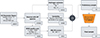 |
Fig. 2. Overview of the selection process with the number of sources at each stage of the selection. |
Constraints and parameter space cuts made for the selection of our candidates.
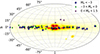 |
Fig. 3. Sky map showing the position of the 67 sources in our initial sample with reference to the Galactic density of stars, constructed with a Gaia DR3 random data set containing 100 000 sources. Different ranges of absolute magnitude are shown with different markers. |
3. Observational data
3.1. Photometry
In optical wavelengths, we retrieved light curves from the Zwicky Transient Facility (ZTF) (Masci et al. 2019), the All Sky Automated Survey for SuperNovae (ASAS-SN) (Hart et al. 2023), the Asteroid Terrestrial-impact Last Alert System (ATLAS) (Tonry et al. 2018; Heinze et al. 2018), and the Transiting Exoplanet Survey Satellite (TESS) (Ricker et al. 2015). In the near-infrared, we retrieved light curves from the NEO Wide-Field Infrared Survey Explorer (NEOWISE) (Mainzer et al. 2011). We cleaned all the photometric data using the recommended flags in the documentation of each catalogue. The TESS processed light curves were retrieved from catalogues that used different reduction pipelines. The main ones used in this work were the TESS Light Curves From Full Frame Images (SPOC) (Caldwell et al. 2020) and the Quick-Look Pipeline (QLP) (Huang et al. 2020; Kunimoto et al. 2021). In addition, we also inspected TESS light curves from the TESS Asteroseismic Science Operations Center (TASOC) (Lund et al. 2021), the TESS FFI-Based Light Curves from the GSFC Team (GSFC-ELEANOR-LITE) (Powell et al. 2022), and the Cluster Difference Imaging Photometric Survey (CDIPS) (Bouma et al. 2019). In Fig. C.1 we show the light curves of all the sources in our sample, in 50-day bins.
3.2. Spectroscopy
Spectra were obtained using the following instruments:
-
The low-resolution instrument CAFOS (Meisenheimer 1994) at the Calar Alto Observatory (CAHA) 2.2 m telescope (Sánchez et al. 2007, 2008), with Grism G-200 (R ∼ 300, 4000–8500 Å). We reduced the data using a custom-developed Python pipeline, adapted by our team.
-
The HERMES high-resolution spectrograph (Raskin et al. 2011) (R = 85 000, 3770–9000 Å) at the Mercator telescope2 (Proposal ID: 5 (ROB service time), PI: Britavskiy, N.). These spectra were flux calibrated using the flux retrieved from the Gaia DR3 low-resolution XP spectra.
-
The FIES instrument (Telting et al. 2014) at the Nordic Optical Telescope (NOT) (Djupvik & Andersen 2010), with the medium-resolution setup (R = 46 000, 3700–8300 Å) and with the low-resolution setup (R = 25 000, 3700–8300 Å) (Proposal ID: P69-854, PI: Wichern, H.; Proposal ID: P70-203, PI: Garcia-Moreno, G.).
-
The ALFOSC instrument at the NOT, with Grism G4 (R = 710 and R = 360, 3200–9600 Å), Grism G7 (R = 650, 3650–7110 Å), and Grism G19 (R = 1940, 4400–6950 Å) (Proposal ID: P70-203, PI: Garcia-Moreno, G.; Proposal ID: P71-209, PI: Blagorodnova, N.). We reduced the data using the Python package PypeIt (Prochaska et al. 2020).
-
Low-resolution (R = 1800, 3700–9000 Å) archival spectra from the Large Sky Area Multi-Object Fibre Spectroscopic Telescope (LAMOST) (Cui et al. 2012).
-
The low-resolution Mookodi spectrograph and imager mounted on the South African Astronomical Observatory (SAAO) 1 m Lesedi telescope (Worters et al. 2016; Erasmus et al. 2024), with a 4″ slit (R ≈ 175, 4 000–8 000 Å). We reduced the data using a Mookodi-specific pipeline developed using the ASPIRED toolkit (Lam et al. 2023), which performs standard long slit reductions including trace fitting, spectral extraction, wavelength calibration and flux calibration.
In Fig. 4 we show single epoch spectra of the 26 candidates that we characterised spectroscopically, and the normalised flux of the Hα and the Hβ profiles in velocity space is shown in Fig. 5. Details of the observations can be found in Table B.2.
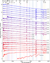 |
Fig. 4. Optical spectra for the subsample of spectroscopically characterised sources. Each spectrum, except for the Mookodi spectrum, is de-reddened for visualisation purposes using the best extinction values (see Sect. 6.1, Table B.1), with Fitzpatrick (1999) dust extinction function and RV = 3.1. The main emission and absorption lines are indicated. The areas with strong telluric absorption are shown by the shaded rectangles. On the right, the number in parentheses indicates the index associated with each source (see Table B.2), and this index is followed by the instrument used to take each spectrum: CAFOS (CAF) from the Calar Alto Observatory 2.2 m telescope, HERMES from the Mercator telescope, FIES and ALFOSC (ALF) from the Nordic Optical Telescope, and Mookodi from the South African Astronomical Observatory 1 m Lesedi telescope. |
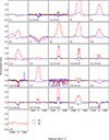 |
Fig. 5. Flux normalised Hα and Hβ velocity profiles for the subsample of observed sources. All sources are shown on the same scale. The index corresponding to each source (see Table B.2) is shown in the bottom left corner of each spectrum. Medium- and high-resolution spectra have been binned using 10 km s−1 bins for improved visual representation. |
4. Analysis
To verify the spectral type and binary nature of our candidates, we performed a light curve analysis and a spectroscopic analysis, in addition to a multi-wavelength characterisation using ultraviolet (UV) and X-ray catalogues from the literature. In this section, we describe the methodology of this analysis.
4.1. Light curve analysis
4.1.1. Visual inspection
We visually inspected the retrieved light curves of every source in our sample. We labelled the observed features in the light curves using the following categories:
-
Different kinds of variability (Diff): sources showing mixed, distinct variability patterns, including different oscillation modes or a combination of periodic and non-periodic variations, for example.
-
Outbursts (Outb): sources showing sudden brightening once or more than once, which could be linked to outbursts.
-
Slow-rising in brightness (SR): sources that are slowly increasing in brightness. This increase can be observed in the optical bands, in the IR bands, or in both. We only give this label to sources that have been increasing in brightness during the observed time frame or are brightening at later times and do not show any signs of a previous brightening.
An example lightcurve for each of these three labels is shown in Fig. 6.
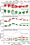 |
Fig. 6. Light curves of three sources in our sample illustrating the types of variability defined in this work (see Sect. 4.1.1). Circles represent the ZTF g band (green) and r band (red), while grey diamonds correspond to the NEOWISE W2 band. For clarity, the g-band and the W2-band light curves are vertically offset in all three panels, and the SR example is binned to better show its long-term evolution. The reference modified Julian date (MJD) corresponds to the start of the ZTF survey. |
4.1.2. Periodicity analysis
We performed a periodicity search using FINKER (Stoppa et al. 2024), a nonparametric kernel regression code, applied to the ZTF, the ASAS-SN, and the ATLAS light curves. Frequencies from 0.001 d−1 (1000 days) to 100 d−1 (14.4 minutes) with steps of 0.0004 d−1 were tested for all sources. Alternative frequency grids were also explored, but they did not yield improved results. We performed an additional search for periods as short as five minutes for some sources where no successful longer period was found. FINKER allows uncertainty estimation in frequency determination via bootstrapping, but in our case, the errors given by this method were insignificant, and we do not report them. Lomb-Scargle periodograms (Lomb 1976; Scargle 1982) were used for TESS light curves, which helped us find the shorter periods in our sample. Lomb-Scargle periodograms were also applied to the ZTF, the ASAS-SN, and the ATLAS light curves, but no significantly better results when compared with FINKER were obtained. In all attempts, we removed data points that were more than 5σ away from the median magnitude of all the observations. Outlier removal was performed carefully to avoid excluding short-duration eclipses. Finally, all periods were tested by visually inspecting the folded light curves.
We labelled the sources based on their periodic variability as sinusoidal (Sin), non-sinusoidal pulsations (Puls), or eclipsing (ECL). Sources were labelled as eclipsing only when the eclipses could be clearly identified. Consequently, contact binaries were classified as sinusoidal variables, since in most cases their eclipses are indistinguishable from the sinusoidal variability of pulsators.
4.2. Spectroscopic analysis
To verify the spectral type of our stars and their location in the HG, we carried out a spectroscopic follow-up campaign targeting the most promising sources with periodic or peculiar light curves. While higher-resolution spectra would allow a more detailed study of specific spectral features, the low resolution obtained for some systems was adequate for our primary objectives: assessing whether the stars are ’yellow’ and verifying the presence of Balmer emission.
4.2.1. Spectroscopic classification
Our sources were given a spectral class by visually inspecting their spectra, and comparing them with theoretical spectra and spectra from standard stars, following Gray & Corbally (2009). We only report temperature types (O-type, B-type, etc.) in our classification, as our only aim is to determine if the spectral type is compatible with being a yellow star. Additionally, to obtain a complementary spectral classification, we used NutMaat (El-Kholy & Hayman 2024), a Python implementation of the MKClass code (Gray & Corbally 2014). These classifications were also compared with the spectral classification provided by Gaia DR3.
4.2.2. Hydrogen line profiles
We inspected the spectral region around Hα and Hβ and labelled each source, given the properties of their hydrogen profiles:
-
P-Cygni profile (PCyg)
-
Emission or absorption in Hα (Hα abs/emi): from the 26 sources with new spectra, this label tells which show emission or absorption in Hα, also indicating if it has a two-peak (2p) profile.
4.2.3. Extinction estimation
For the spectra with the high and medium resolution, we estimated the extinction from the absorption caused by the diffuse interstellar bands (DIBs) at 5780 Å and 6614 Å following Carvalho & Hillenbrand (2022), where they derive an empirical relation between the line-of-sight extinction and the EW of these two DIBs. To convert line-of-sight extinctions to visual extinctions, we used RV = AV/E(B − V) = 3.1. The resulting AV values were then converted to extinctions in the Gaia passbands using the gaia_edr3_photutils package3. To use this method, we needed precise measurements of the EWs of the DIBs, which we could not get with our low-resolution spectra.
4.3. Characterisation with auxiliary catalogues
We cross-matched our sample with the UV catalogue GALEX (Martin et al. 2005) (with a search radius of 10 arcseconds), and X-ray catalogues from Swift (Evans et al. 2020) (with a search radius of 10 arcseconds), Chandra (Evans et al. 2010) (with a search radius of 50 arcseconds), eROSITA (Merloni et al. 2024) (with a search radius of 10 arcseconds), and 4XMM (Webb et al. 2020) (with a search radius of 12 arcseconds). In all cases, the search radius was chosen to be enough to contain the positional error of the catalogues. We labelled the sources with X-ray (Hard X-ray) or UV (Far UV) detections.
To test for known variable stars, we also cross-matched our sample with a catalogue containing a cross-match of over 8 million Gaia sources with variable objects in 152 different catalogues from the literature (Gavras et al. 2023, or GVXM from now on). This catalogue provides over 100 variability (sub)types and periods, if available.
5. Results
5.1. Light curve analysis
We observe variability in the light curves of all 67 sources in our sample, but not all show signs of periodicity. Among all the sources, 19 show multiple types of variability, the majority of them likely associated with more than one pulsation mode (e.g. sources 2164630463117114496 or 4281886474885416064); ten show a fast decrease in magnitude (e.g. sources 526939882463713152 or 2027563492489195520), and 11 sources present a slow increase in brightness over several hundreds or thousands of days (e.g. source 4263591911398361472). For some of the latter, the gradual brightening may be linked to long-term variability; future light curve data will help determine whether this is the case.
The folded light curves of the 36 candidates for which we determined a period are shown in Fig. C.2 and Fig. C.3. Periods of one day or less were found for 19 candidates, periods between one and eight days for ten candidates, and periods longer than ten days for the remaining seven, with the longest period being ≈106.76 days. Among these 36 sources with periodic variability, 26 show sinusoidal variability, nine show eclipses, and we identify pulsations for one (see Fig. 7).
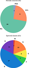 |
Fig. 7. Top: Pie chart with the types of periodic variables identified in our sample. Bottom: Pie chart with the spectral classes in our sample, combining the results of our classification and the classes reported in the Gaia DR3. |
We note that periods detected exclusively in TESS light curves should be interpreted with caution. Given the large plate scale of TESS (21″ pixel−1), light curve contamination from nearby bright variables is possible when sources lie within the same pixel. This is a known issue discussed, for example, by Pedersen & Bell (2023) in the context of fast yellow pulsating supergiants. In our case, the short period of ≈0.171 days initially found for source 5962956195185292288 using TESS data was later traced to an eclipsing binary located ≈42″ away, identified as Gaia DR3 5962956229545027712.
5.2. Spectroscopic analysis
The estimated spectral types we report from our visual inspection can be grouped into three main groups: hotter stars (O- and B-type), yellow stars (F- and G-type), and colder stars (K- or M-type). Out of the 26 candidates with spectra, we identified 17 as hotter stars, most of them Be stars. On the other side, we identified one source as a K-type star, and one as an M-type star. Overall, only four sources were finally assigned a spectral type compatible with being a YG or YSG: three F-type stars and one G-type star. The spectra obtained for three of the sources showed no clear features (apart from the main hydrogen lines), and we did not assign a spectral class to them. The NutMaat classifications rated as ’good’ or better were consistent with our spectroscopic results, yielding the same temperature types as those we derived.
A comparison of our spectral classification with the one available in the Gaia DR3 showed consistent results for 18 stars. For two, Gaia identified them as G-type stars, whereas we classified them as B-type based on the presence of He I absorption lines. Another source was classified as an O-type star by Gaia, but our analysis indicates that its spectrum matches a B-type better. Additionally, Gaia had spectral types for 38 sources in our sample for which we lacked spectra. These 38 spectral types are distributed as follows: 8 O-type, 13 B-type, 2 F-type, 5 G-type, and 10 K-type stars. All the spectral types identified are summarised in Fig. 7.
We note that our spectral classification was based on single stellar spectra. In the case of binaries, this approach is reasonable when one component dominates the system’s light, which we consider to be the case for our sources. Indeed, most of our spectra showed no evidence of composite features, suggesting that the contribution of a secondary component is negligible. However, this effect could explain the peculiar spectra observed in the three candidates for which no spectral type was assigned (sources 2061252975440642816, 2164630463117114496, and 2175699216614191360).
From the Hα and Hβ profiles shown in Fig. 5, we identified Hα emission in 19 sources (ten of which had a two-peak profile), Hα absorption in five sources, and no discernible features in two of them. Five sources had Hβ emission in addition to Hα emission. Additionally, in Fig. C.4 we present a comparison between the Hα profiles obtained from the Gaia XP low-resolution spectra and our follow-up spectra, degraded to match the XP resolution. In most cases, the profiles show good agreement, while in others they differ significantly, suggesting that the Hα emission may be transitory or variable over time.
Following the method described in Sect. 4.2.3, we estimated the extinction for each source, resulting in AV values reported in Table 2. Updated extinction values have enabled us to revisit the locations of nine sources in the Gaia colour-magnitude diagram, as shown in Fig. 8. The discussion of these results and a comparison of our extinction estimates with those from two external catalogues are discussed in Sections 6.1 and 6.2.
Results of our extinction estimates using diffuse interstellar bands (DIBs).
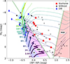 |
Fig. 8. Positions of the nine sources for which we re-estimated extinction (see Sect. 4.2.3) in the colour-magnitude diagram. Red squares indicate the positions derived using StarHorse, while blue diamonds show the positions computed using our extinction estimates based on diffuse interstellar bands, averaging the results from the 5780 Å and 6614 Å lines. For comparison, we also show the positions of all sources in our sample using the SHBoost catalogue (black stars; see Sect. 6.1). The schematic boxes denote the typical locations of different stellar types. |
5.3. Characterisation with auxiliary catalogues
Our cross-match with UV and X-ray catalogues allowed the identification of three sources with X-ray emission, and one source with UV excess. The source with the UV detection in GALEX was 6123873398383875456, which presented UV excess in the far UV channel (1350–1750 Å). This detection matched the optical counterpart at 0.44 arcseconds (within positional errors and with no other optical counterpart nearby).
The X-ray detections came from 4XMM and Swift: one detection in Swift’s 2SXPS catalogue matching source 4054010697162430592 at 0.93 arcseconds (within positional errors and with no other optical counterpart nearby), and two detections in 4XMM-DR14, matching source 5866345647515558400 at 1.1 arcseconds and source 2083649030845658624 at 1.9 arcseconds, with both within positional errors. However, 2083649030845658624 had other optical counterparts within a few arcseconds (also within positional errors), so it is not clear if the X-ray emission is from our source.
Our search for periods reported in the literature provided 18 catalogued periods. Comparing these with the periods derived in this work, we found that eight sources had consistent values. For one eclipsing binary, our analysis yielded half the reported period. We were able to reproduce the reported period for four sources, while for the remaining five, the periods published in GVXM could not be confirmed with our data. The unconfirmed periods correspond to relatively long timescales, which may not be reproduced with our data either due to the limited observational baseline or because the literature periods themselves are uncertain, as the cross-matched values in GVXM are not independently verified.
The main results of our photometric and spectroscopic analysis are summarised in Fig. 7, and all the results of our analysis are provided in Table B.3, where we present the spectral types identified in this work together with the types listed by Gaia, the main properties in the light curves and the spectra, the classes from the literature (from the GVXM and SIMBAD), and the periods found in this work and the literature. Literature periods that could not be confirmed with our data are marked with an asterisk in the last column of these tables.
6. Discussion
The goal of our selection was to identify mass-transferring binaries in the HG. However, our sample includes a variety of spectral types, most of which are contaminants. In this section, we first discuss how line-of-sight extinction affected our selection process, and then examine the nature of our candidates.
6.1. The effect of extinction
The most significant limitation of our method for selecting our sample of HG stars was the lack of reliable extinction estimates in the literature. As a result, for more than half of the sources in our sample, the extinction was underestimated, implying that the MS O- and B-type sources appeared fainter and redder. Consequently, many of our candidates were stars such as Oe or Be stars, which share some characteristics with our objects of interest but are generally not expected to lie in the HG Cochetti et al. (2020). Therefore, obtaining precise extinction estimates is essential for reliably selecting sources within the narrow region of the colour-magnitude diagram occupied by the HG.
Luckily, during the preparation of this work, several new astrophysical parameter catalogues derived from Gaia XP spectra became available (e.g. Zhang et al. 2023; Fallows & Sanders 2024; Huson et al. 2025). Of particular interest for us was the new SHBoost catalogue (Khalatyan et al. 2024), which contains stellar parameters (effective temperature, surface gravity, mass, metallicity) and line-of-sight extinctions computed using Gaia DR3 XP spectra, derived through supervised machine learning trained on a large high-quality dataset comprising the StarHorse results for spectroscopic stellar surveys (Queiroz et al. 2023) as well as complementary datasets of hot stars, white dwarfs, hot subdwarfs, among others. Particularly relevant for this work is that SHBoost contains more reliable characterisation (including extinction) for high-mass stars than the StarHorse catalogue, based on Gaia EDR3.
6.2. Revisiting our first selection with SHBoost
To assess the position of our sources in the colour-magnitude diagram with better extinction values, we cross-matched our sample with the SHBoost catalogue to obtain more accurate absolute magnitudes and colours. A comparison with the extinction corrected magnitudes from DIB spectroscopy is shown in Fig. 8, where we highlight two key observations: first, many of the Oe and Be stars now lie on the MS or just beyond the terminal-age MS, while the cooler stars (K- and M-types) are located on the RGB; second, all but one of the extinction values derived from our spectroscopic analysis are higher than those reported in SHBoost, with AV values larger by approximately 0.7 mag on average. However, the values remain comparable within uncertainties, and we therefore consider the SHBoost estimates to be reliable. Figure 8 also shows that from the initial 67 candidates selected based on the EDR3 StarHorse catalogue, only 25 remain in our HG parameter space. Given these results, we can now discuss the true nature of the sources in our sample.
6.3. Nature of our candidates
6.3.1. Oe and Be stars
Oe and Be stars are rapidly rotating, moderately massive stars (M ∼ 3.6–20 M⊙) with Balmer emission associated with a gaseous envelope, and with an equatorial disk likely formed through pulsations or by radiatively driven winds (Porter & Rivinius 2003; Rivinius et al. 2013). Moreover, these stars show IR excess caused by free–free and free–bound emission from the gas in the disk (Gehrz et al. 1974). Oe and Be stars are also known to exhibit different kinds of photometric variability (Diago et al. 2009; Labadie-Bartz et al. 2017).
Among the O- and B-type stars identified in our sample, 15 are strong candidates for Oe or Be stars based on the presence of Balmer emission. In some cases, Oe and Be stars also display Ca II triplet and Paschen emission (e.g. Polidan 1976; Banerjee et al. 2021), an emission we identify in, for example, sources 2013187240507011456 and 2074693061975359232. Only two B-type stars in our sample do not show Balmer emission in our follow-up spectra. As noted by Negueruela et al. (2004), the emission lines in Oe and Be stars are variable and can transition from emission to absorption as the star temporarily exits the Be phase. This may explain the case of source 508419369310190976, for which Hα emission is visible in the Gaia XP spectrum (see Fig. C.4), but it is absent in our follow-up spectrum.
Additionally, for the 44 sources for which we could not assign a spectral classification, either because we did not have follow-up spectra or because the spectra did not show enough features, 21 were classified as O- or B-type stars by Gaia. Based on the selection criteria of our search and the results obtained, there is a strong reason to believe that most, if not all, of these sources are Oe or Be stars.
6.3.2. Regular variables
Regular variables cannot be discarded as possible contaminants in our search. We discuss source 6123873398383875456 in Sect. 6.3.4, which we think is most likely a close binary misclassified as an RRc, but we found two other sources classified as regular pulsator stars in the literature: 460686648965862528, classified as a δ Scuti by Chen et al. (2020), and 4076568861833452160, classified as a Cepheid by Jayasinghe et al. (2019). These kinds of variables reside in the instability strip, which crosses the HG, so it is expected to find them in our parameter space. Examples of different kinds of variables placed in the Gaia HR diagram can be found in Gavras et al. (2023).
Mid-IR excess is also expected in Cepheid variables (Kervella et al. 2006; Hocdé et al. 2020), and Balmer emission has been observed in the type II Cepheid W Virginis (Kovtyukh et al. 2011). Pre-MS δ Scuti variable stars have been observed before (Díaz-Fraile et al. 2014), and strong IR-excess and emission are expected in this type of star, linked to active accretion processes. Therefore, the selection of these variables with our search criteria is possible, and a new identification method will be needed to trace and remove them from our sample, especially if we want to distinguish them from close binaries, which can have similar light curves.
6.3.3. Binaries with compact companions
As described in Sect. 5.3, we identify one source with far UV excess and three sources with hard X-ray emission. From the three sources with X-ray detections, it is not clear if the X-ray detection of source 2083649030845658624 corresponds to its optical counterpart, whereas sources 4054010697162430592 (reported as a single-lined spectroscopic binary in Makarov & Unwin 2015) and 5866345647515558400 are good candidates for X-ray binaries.
Interestingly, the source with far UV excess–source 473575777103322496–is identified as a Be star, has sinusoidal variability with a period of 0.45878 days (Fig. C.3), and shows two peaks in the IR light curve, one between 2014 and 2016 and a second one between 2018 and 2020 (Fig. C.1). We suggest this source is a Be star with a hot companion (a subdwarf OB star or a white dwarf, for example), which is potentially accreting mass during a second mass transfer stage (as discussed in Gies et al. 2023 for γ Cas stars), based on the UV emission and the observed variability.
6.3.4. Mass transferring systems
One possible method for assessing whether our candidates were undergoing mass transfer in a binary system was to compare their observed orbital period with the theoretical period at which Roche lobe overflow would occur (PRLO). Therefore, we take advantage of the improved parameters given by SHBoost to calculate this period,
 (1)
(1)
The masses are provided directly by SHBoost, while the radii are computed using the log g values also given in SHBoost. We adopted a fixed mass ratio of q = 0.5 but accounting for the dependence on q in the error bars by also computing the period at q = 0.01 (indicating that 99% of the system’s mass resides in the primary star) and at q = 1 (representing an equal-mass binary). The dependence of PRLO on q is weak, and adopting different q values does not significantly affect our results. It is to be noted that the masses in SHBoost are computed assuming single stars. In case the second component contributes to the total light, this may affect the final PRLO, adding an additional uncertainty that we can not verify straightforwardly.
We compared the PRLO to the periods found in this work, and we show this in Fig. 9, where we also mark different kinds of variables found among our candidates, their spectral class, and whether they remain in the HG using the extinctions from the SHBoost catalogue. Points above the diagonal correspond to sources with an observed period shorter than the period they would have if they were a binary and one of the components had filled its Roche lobe, whereas the opposite is true for points below the diagonal. Binaries in this region, with observed periods longer than PRLO, are most likely detached binaries. Nonetheless, an interesting example of a source in this area–the G-type star 2060841448854265216–shows, in its folded light curve, eclipses akin to an Algol star with an accretion disk around the gainer (see C.2). Algol binaries are systems where the mass gainer is the more massive star that is still in the MS, and the donor is the cooler, fainter and larger star (Peters 2001). In this case, we could be seeing the less evolved star (or a combination of the two), which would mean PRLO is underestimated. Consequently, we would not rule out 2060841448854265216 as a potential mass-transferring binary.
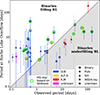 |
Fig. 9. Comparison of the observed period and the theoretical period of a binary in which one star fills its Roche lobe (see Sect. 6.3.4). Different marker shapes correspond to different types of stars, and colours represent spectral classes (using our classification when available, and Gaia’s otherwise). Sources that lie, based on SHBoost values, within our defined HG parameter space are highlighted with circles. |
The most relevant sources for our study are those located near the line where the observed period equals PRLO, as these represent the strongest candidates for ongoing mass transfer in binary systems. Among them, perhaps the most intriguing is source 6228685649971375616, a yellow HG star with a folded light curve characteristic of an interacting binary and an orbital period of 1.274 days. The light curves in different bands are shown in Fig. 10, together with the folded ATLAS o-band and ZTF g-band light curves. We also present the Gaia XP spectrum and compare it with a model spectrum of a late F-type star (Teff = 6100 K). The model was generated using pysynphot (STScI Development Team 2013) with the Castelli–Kurucz Atlas (Castelli et al. 2003), adopting log g = 3.75, as reported by SHBoost (see Table B.1). The comparison shows a good agreement between the observed and model spectra, confirming that this is indeed a yellow source. Although no clear Hα emission is detected in the Gaia XP spectrum, the absence of a well-defined absorption feature suggests that the expected absorption is partially filled.
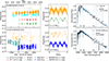 |
Fig. 10. Light curve (left column), phase-folded light curve (middle column), and spectrum (right column) of our two best candidates for mass-transferring merger progenitors: 6228685649971375616 (top row) and 6123873398383875456 (bottom row). For both sources, a model spectrum from the Castelli–Kurucz Atlas (Castelli et al. 2003), with Teff = 6100 K and log g = 3.75, is shown for comparison. The ZTF and NEOWISE data in the light curves (left column) are offset for visual clarity, and the reference modified Julian date (MJD) in the light curve corresponds to the start of observations by ZTF. Although we report a sinusoidal period of 0.39674 d for 6123873398383875456, the phase-folded light curve is shown using twice this period, consistent with our interpretation of the source as a contact eclipsing binary. The ⊕ symbols and shaded areas in the spectra (right column) represent telluric absorption (absorption by the Earth’s atmosphere). |
If this source is indeed evolving towards a merger (and a subsequent LRN), and assuming its progenitor behaves similarly to that of V1309 Sco (Tylenda et al. 2011), we would expect to observe three key signatures in its light-curve evolution: (1) a steady, monotonic brightening over several years (of ≈1 mag in the I band for V1309 Sco) prior to outburst; (2) a progressive decrease in the orbital period as the components spiral in; and (3) a transition in the folded light-curve morphology from an EW-type with two maxima per cycle to an asymmetric single maxima profile (see Figures 1–3 in Tylenda et al. 2011). Such behaviour is not observed in 6228685649971375616. A slight increase in brightness is seen in the ATLAS bands (of about 0.1 mag over approximately 10 years), but this trend is not evident in other bands. Moreover, we detect no significant evolution in the folded light curve, which consistently shows two maxima and two minima per cycle across all epochs. We measured the period across different epochs, but any variations detected were smaller than the associated uncertainties. Investigating potential period evolution would require high-cadence observations over an extended timespan, which are not available for this source. If this object is indeed similar to the progenitor of V1309 Sco, we do not expect its outburst to occur in the near future.
While for the source discussed above we could clearly distinguish the two minima corresponding to the eclipses, this is not the case for some contact binaries. Contact binaries and regular pulsators can exhibit similarly sinusoidal light curves with short periods. Therefore, some of our candidates showing sinusoidal variability may in fact be close binary systems. One such case is 6123873398383875456, an F-type star identified in the ASAS-SN catalogue of variable stars (Jayasinghe et al. 2019) as an RRc-type pulsator, although it is not included in the RR Lyrae table of Gaia DR3. Notably, this source has a re-normalised unit weight error (RUWE) of nearly 6.5 in the Gaia DR3 catalogue, a value well above the nominal threshold and often indicative of unresolved binarity (Castro-Ginard et al. 2024). The folded light curve displays two symmetric minima with slightly different depths but the same periodicity. Although this behaviour could be attributed to period doubling in an RR Lyrae star, it could also correspond to the two eclipses of a contact binary. If the latter interpretation is correct, the star would lie just above the 1:1 line in Fig. 9, further supporting the hypothesis that it is a mass-transferring binary.
Similarly to 6228685649971375616, source 6123873398383875456 does not show the behaviour expected for an LRN progenitor approaching outburst. In Fig. 10, we show its light curves across different bands, along with the folded ATLAS o-band and ASAS-SN g-band light curves. We also present the follow-up spectrum, which we compare to a model of a late F-type star (the same model described above).
The case of source 6228685649971375616, however, appears to be an exception rather than the rule, as we do not find any evidence of binarity in other sinusoidal sources. As discussed in the subsections above, regular variables and OBe stars can also be selected by our criteria. These likely account for the majority of stars with sinusoidal light curves located in the leftmost region of the PRLO-observed period diagram.
Interestingly, among all the O- and B-type stars in our sample, we identify at least seven in binary systems, including three Be stars: 527155253604491392, 2006088484204609408, and 2166378312964576256. The formation channel of Oe and Be stars remains a topic of debate, although several studies suggest that close binary interactions are an important channel for their formation (e.g. Pols et al. 1991; Shao & Li 2014; Dodd et al. 2024). These three Be stars in binary systems are therefore particularly compelling targets for investigating this formation channel. Two of them–527155253604491392 and 2166378312964576256–appear to be in wide binaries, possibly having acquired their Be characteristics through past binary interaction, as suggested by their location in Fig. 9. In contrast, 2006088484204609408 may represent an actively interacting binary system, where the accreting star is currently evolving into a Be star.
7. New sample of HG objects
The analysis of our initial sample showed that uncertainties in the extinction were the main cause of including contaminants in our selection process. Given the appearance of new catalogues, we redid the same selection steps described in Sect. 2, but this time on the SHBoost input catalogue instead of StarHorse. In this case, we only looked at Hα EW values for the selection of hydrogen emitters, and we removed false positives by visual inspection of the calibrated XP spectra. We did not remove any further sources that might have a classification in SIMBAD or other catalogues. The other selection steps were kept the same.
The filtering process provided a new preliminary sample composed of 444 sources. After visually inspecting the XP spectra of the preliminary sample, we finished with a new sample composed of 308 HG stars that fit our criteria. We will explore this new sample in future research. We present this new sample in a table made available in its entirety via CDS/VizieR.
8. Summary and conclusions
In this work, we aimed to identify Galactic mass-transferring binaries with quickly evolving donors in the HG with yellow spectral types that showed Balmer emission, mid-IR excess, and variability. After our initial selection, we obtained a sample of 67 candidates that we analysed using photometric data and spectroscopic data, along with multi-wavelength photometric archival data. We present a summary of the nature of our candidates (identified by their Gaia DR3 IDs):
-
We computed periods for 36 sources, among which 26 showed sinusoidal variability, nine were eclipsing binaries, and one showed pulsations.
-
The spectral types we identified from our follow-up spectra and the spectral types given by Gaia were in agreement in 18 out of 21 cases. Combining our spectral types and the ones reported by Gaia, the distribution of spectral classes in our sample was: 11 O-type, 27 B-type, 5 F-type, 6 G-type, 11 K-type, and 1 M-type star.
-
Among the O- and B-type stars in our sample, 15 are strong candidates for Oe or Be stars based on the presence of Balmer emission. These reddened Oe and Be stars contributed the most to the contaminants in our sample.
-
Regular variables cannot be discarded as possible contaminants, and we identified two in our sample: a δ Scuti (460686648965862528), and a Cepheid (4076568861833452160).
-
Three sources in our sample showed associated hard X-ray emission. Two of them had good matches with their optical counterpart (sources 4054010697162430592 and 5866345647515558400), and are strong candidates for X-ray binaries. Source 2083649030845658624 had other optical counterparts within the positional errors of the X-ray detection.
-
Source 473575777103322496 shows far UV excess. This source was identified as a Be star, and we suggest it is in a binary system with a hot companion (subdwarf OB star or a white dwarf, for example), and it is potentially mass-transferring.
-
The strongest candidates for mass-transferring binaries with a bright yellow primary are 2060841448854265216, a G-type star whose light curve resembles that of an Algol-type eclipsing binary with an accretion disk; 6228685649971375616, an F-type star in a close binary, and 6123873398383875456, an F-type contact binary that was previously misclassified as an RRc Lyrae star.
-
Among all the O- and B-type stars in our sample, we identify seven in binary systems, including three Be stars: 527155253604491392, 2006088484204609408, and 2166378312964576256. These three Be stars in binary systems are particularly compelling targets for investigating the formation channel of Oe and Be stars through close binary interactions.
Most of the sources in our analysed sample are not yellow stars. Of the initial 67 candidates selected using the EDR3 StarHorse catalogue, only 25 remain within our HG parameter space when using the more reliable SHBoost extinction values. This underscores a key challenge in our original goal of identifying yellow HG stars as potential LRN progenitors: the large uncertainties in extinction estimates from Gaia and StarHorse, which were central to defining our selection space.
Comparing the observations of the two best candidates for stellar-merger progenitors in our sample–6228685649971375616 and 6123873398383875456–with those of the progenitor of V1309 Sco, the best-studied case of a stellar merger to date, suggests that if these systems are indeed potential merger progenitors, they are still far from the merger phase. Nevertheless, both remain interesting targets that deserve further investigation.
As an additional outcome of this work, we present a refined selection of 308 HG candidate stars using the improved extinction correction from the SHBoost catalogue. This new sample was derived using the same overall methodology but incorporates improved extinction estimates and visual inspection of the Gaia XP spectra, ensuring that each selected object displays, at a minimum, clear Hα emission. From this revised sample, we expect to identify a significantly larger fraction of scientifically valuable mass-transferring binary systems.
This new sample gives new opportunities to explore HG stars with interesting features. We encourage other teams to pursue follow-up observations of promising sources in this newly identified sample, and also of interesting sources in our initial sample. Additionally, forthcoming data releases, particularly Gaia DR4, expected by the end of 2026, will substantially enhance the search for HG mass-transferring binaries by providing improved spectrophotometric and astrometric data, including BP/RP spectra for all sources down to G ≈ 19 mag, RVS spectra for sources brighter than G ≈ 14.5 mag, and epoch photometry. These additions will offer a richer dataset for identifying and characterising evolved binaries and their emission features with greater precision.
Data availability
The new HG sample presented in Sect. 7 is available at the CDS via https://cdsarc.cds.unistra.fr/viz-bin/cat/J/A+A/706/A249
References
- Addison, H., Blagorodnova, N., Groot, P. J., et al. 2022, MNRAS, 517, 1884 [NASA ADS] [CrossRef] [Google Scholar]
- Anders, F., Khalatyan, A., Queiroz, A. B. A., et al. 2022, A&A, 658, A91 [NASA ADS] [CrossRef] [EDP Sciences] [Google Scholar]
- Andrew, S., Swihart, S. J., & Strader, J. 2021, ApJ, 908, 180 [NASA ADS] [CrossRef] [Google Scholar]
- Armeni, A., & Shore, S. N. 2022, A&A, 664, A103 [NASA ADS] [CrossRef] [EDP Sciences] [Google Scholar]
- Astropy Collaboration (Price-Whelan, A. M., et al.) 2022, ApJ, 935, 167 [NASA ADS] [CrossRef] [Google Scholar]
- Banerjee, G., Mathew, B., Paul, K. T., et al. 2021, MNRAS, 500, 3926 [Google Scholar]
- Blagorodnova, N., Kotak, R., Polshaw, J., et al. 2017, ApJ, 834, 107 [NASA ADS] [CrossRef] [Google Scholar]
- Blagorodnova, N., Klencki, J., Pejcha, O., et al. 2021, A&A, 653, A134 [NASA ADS] [CrossRef] [EDP Sciences] [Google Scholar]
- Bond, H. E., Henden, A., Levay, Z. G., et al. 2003, Nature, 422, 405 [CrossRef] [Google Scholar]
- Bouma, L. G., Hartman, J. D., Bhatti, W., Winn, J. N., & Bakos, G. Á. 2019, ApJS, 245, 13 [Google Scholar]
- Brož, M., Mourard, D., Budaj, J., et al. 2021, A&A, 645, A51 [EDP Sciences] [Google Scholar]
- Cai, Y. Z., Pastorello, A., Fraser, M., et al. 2022, A&A, 667, A4 [Google Scholar]
- Caldwell, D. A., Tenenbaum, P., Twicken, J. D., et al. 2020, Res. Notes Am. Astron. Soc., 4, 201 [Google Scholar]
- Carrasco, J. M., Weiler, M., Jordi, C., et al. 2021, A&A, 652, A86 [NASA ADS] [CrossRef] [EDP Sciences] [Google Scholar]
- Carvalho, A. S., & Hillenbrand, L. A. 2022, ApJ, 940, 156 [NASA ADS] [CrossRef] [Google Scholar]
- Castelli, F., & Kurucz, R. L. 2003, in Modelling of Stellar Atmospheres, eds. N. Piskunov, W. W. Weiss, & D. F. Gray, IAU Symp., 210, A20 [Google Scholar]
- Castro-Ginard, A., Penoyre, Z., Casey, A. R., et al. 2024, A&A, 688, A1 [NASA ADS] [CrossRef] [EDP Sciences] [Google Scholar]
- Cehula, J., & Pejcha, O. 2023, MNRAS, 524, 471 [NASA ADS] [CrossRef] [Google Scholar]
- Chen, X., Wang, S., Deng, L., et al. 2020, ApJS, 249, 18 [NASA ADS] [CrossRef] [Google Scholar]
- Cochetti, Y. R., Zorec, J., Cidale, L. S., et al. 2020, A&A, 634, A18 [EDP Sciences] [Google Scholar]
- Crawford, J. A. 1955, ApJ, 121, 71 [NASA ADS] [CrossRef] [Google Scholar]
- Cui, X.-Q., Zhao, Y.-H., Chu, Y.-Q., et al. 2012, Res. Astron. Astrophys., 12, 1197 [Google Scholar]
- Cutri, R. M., Wright, E. L., Conrow, T., et al. 2021, VizieR Online Data Catalog, II/328 [Google Scholar]
- De Angeli, F., Weiler, M., Montegriffo, P., et al. 2023, A&A, 674, A2 [NASA ADS] [CrossRef] [EDP Sciences] [Google Scholar]
- de Mink, S. E., Sana, H., Langer, N., Izzard, R. G., & Schneider, F. R. N. 2014, ApJ, 782, 7 [Google Scholar]
- Diago, P. D., Gutiérrez-Soto, J., Auvergne, M., et al. 2009, A&A, 506, 125 [NASA ADS] [CrossRef] [EDP Sciences] [Google Scholar]
- Díaz-Fraile, D., Rodríguez, E., & Amado, P. J. 2014, A&A, 568, A32 [NASA ADS] [CrossRef] [EDP Sciences] [Google Scholar]
- Djupvik, A. A., & Andersen, J. 2010, in Highlights of Spanish Astrophysics V, Astrophys. Space Sci. Proc., 14, 211 [NASA ADS] [CrossRef] [Google Scholar]
- Dodd, J. M., Oudmaijer, R. D., Radley, I. C., Vioque, M., & Frost, A. J. 2024, MNRAS, 527, 3076 [Google Scholar]
- Dotter, A. 2016, ApJS, 222, 8 [Google Scholar]
- El-Kholy, R. I., & Hayman, Z. M. 2024, NutMaat: A Python library for classifying stellar spectra based on the MKCLASS package [Google Scholar]
- Erasmus, N., Steele, I. A., Piascik, A. S., et al. 2024, J. Astron. Telesc. Instrum. Syst., 10, 025005 [Google Scholar]
- Evans, I. N., Primini, F. A., Glotfelty, K. J., et al. 2010, ApJS, 189, 37 [NASA ADS] [CrossRef] [Google Scholar]
- Evans, P. A., Page, K. L., Osborne, J. P., et al. 2020, ApJS, 247, 54 [Google Scholar]
- Fallows, C. P., & Sanders, J. L. 2024, MNRAS, 531, 2126 [CrossRef] [Google Scholar]
- Fitzpatrick, E. L. 1999, PASP, 111, 63 [Google Scholar]
- Gaia Collaboration (Prusti, T., et al.) 2016, A&A, 595, A1 [NASA ADS] [CrossRef] [EDP Sciences] [Google Scholar]
- Gaia Collaboration (Brown, A. G. A., et al.) 2018, A&A, 616, A1 [NASA ADS] [CrossRef] [EDP Sciences] [Google Scholar]
- Gaia Collaboration (Brown, A. G. A., et al.) 2021, A&A, 649, A1 [NASA ADS] [CrossRef] [EDP Sciences] [Google Scholar]
- Gaia Collaboration (Vallenari, A., et al.) 2023, A&A, 674, A1 [NASA ADS] [CrossRef] [EDP Sciences] [Google Scholar]
- Gavras, P., Rimoldini, L., Nienartowicz, K., et al. 2023, A&A, 674, A22 [NASA ADS] [CrossRef] [EDP Sciences] [Google Scholar]
- Gehrz, R. D., Hackwell, J. A., & Jones, T. W. 1974, ApJ, 191, 675 [Google Scholar]
- Gies, D. R., Wang, L., & Klement, R. 2023, ApJ, 942, L6 [NASA ADS] [CrossRef] [Google Scholar]
- Ginsburg, A., Sipőcz, B. M., Brasseur, C. E., et al. 2019, AJ, 157, 98 [Google Scholar]
- Gray, R. O., & Corbally, C. J. 2009, Stellar Spectral Classification (Princeton University Press) [Google Scholar]
- Gray, R. O., & Corbally, C. J. 2014, AJ, 147, 80 [CrossRef] [Google Scholar]
- Harris, C. R., Millman, K. J., van der Walt, S. J., et al. 2020, Nature, 585, 357 [NASA ADS] [CrossRef] [Google Scholar]
- Hart, K., Shappee, B. J., Hey, D., et al. 2023, arXiv e-prints [arXiv:2304.03791] [Google Scholar]
- Heinze, A. N., Tonry, J. L., Denneau, L., et al. 2018, AJ, 156, 241 [Google Scholar]
- Hocdé, V., Nardetto, N., Lagadec, E., et al. 2020, A&A, 633, A47 [NASA ADS] [CrossRef] [EDP Sciences] [Google Scholar]
- Huang, C. X., Vanderburg, A., Pál, A., et al. 2020, Res. Notes Am. Astron. Soc., 4, 204 [Google Scholar]
- Hunter, J. D. 2007, Comput. Sci. Eng., 9, 90 [NASA ADS] [CrossRef] [Google Scholar]
- Huson, D., Cowan, I., Sizemore, L., Kounkel, M., & Hutchinson, B. 2025, ApJ, 984, 58 [Google Scholar]
- Ivanova, N., & Taam, R. E. 2004, ApJ, 601, 1058 [Google Scholar]
- Ivanova, N., Podsiadlowski, P., & Spruit, H. 2001, in Evolution of Binary and Multiple Star Systems, eds. P. Podsiadlowski, S. Rappaport, A. R. King, F. D’Antona, & L. Burderi, ASP Conf. Ser., 229, 261 [Google Scholar]
- Jayasinghe, T., Stanek, K. Z., Kochanek, C. S., et al. 2019, MNRAS, 485, 961 [Google Scholar]
- Kahraman Aliçavuş, F., Handler, G., Aliçavuş, F., et al. 2022, MNRAS, 510, 1413 [Google Scholar]
- Kato, T. 2003, A&A, 399, 695 [NASA ADS] [CrossRef] [EDP Sciences] [Google Scholar]
- Kervella, P., Mérand, A., Perrin, G., & Coudé du Foresto, V. 2006, A&A, 448, 623 [NASA ADS] [CrossRef] [EDP Sciences] [Google Scholar]
- Khalatyan, A., Anders, F., Chiappini, C., et al. 2024, A&A, 691, A98 [NASA ADS] [CrossRef] [EDP Sciences] [Google Scholar]
- Kovtyukh, V. V., Wallerstein, G., Andrievsky, S. M., et al. 2011, A&A, 526, A116 [NASA ADS] [CrossRef] [EDP Sciences] [Google Scholar]
- Kraft, R. P. 1964, ApJ, 139, 457 [Google Scholar]
- Kuiper, G. P. 1941, ApJ, 93, 133 [NASA ADS] [CrossRef] [Google Scholar]
- Kunimoto, M., Huang, C., Tey, E., et al. 2021, Res. Notes Am. Astron. Soc., 5, 234 [Google Scholar]
- Labadie-Bartz, J., Pepper, J., McSwain, M. V., et al. 2017, AJ, 153, 252 [NASA ADS] [CrossRef] [Google Scholar]
- Lam, M. C., Smith, R. J., Arcavi, I., et al. 2023, AJ, 166, 13 [NASA ADS] [CrossRef] [Google Scholar]
- Lomb, N. R. 1976, Ap&SS, 39, 447 [Google Scholar]
- Lund, M. N., Handberg, R., Buzasi, D. L., et al. 2021, ApJS, 257, 53 [NASA ADS] [CrossRef] [Google Scholar]
- MacLeod, M., Macias, P., Ramirez-Ruiz, E., et al. 2017, ApJ, 835, 282 [NASA ADS] [CrossRef] [Google Scholar]
- Mainzer, A., Bauer, J., Grav, T., et al. 2011, ApJ, 731, 53 [Google Scholar]
- Maíz Apellániz, J., Holgado, G., Pantaleoni González, M., & Caballero, J. A. 2023, A&A, 677, A137 [NASA ADS] [CrossRef] [EDP Sciences] [Google Scholar]
- Makarov, V. V., & Unwin, S. C. 2015, MNRAS, 446, 2055 [NASA ADS] [CrossRef] [Google Scholar]
- Marchant, P., Pappas, K. M. W., Gallegos-Garcia, M., et al. 2021, A&A, 650, A107 [NASA ADS] [CrossRef] [EDP Sciences] [Google Scholar]
- Martin, D. C., Fanson, J., Schiminovich, D., et al. 2005, ApJ, 619, L1 [Google Scholar]
- Martini, P., Wagner, R. M., Tomaney, A., et al. 1999, AJ, 118, 1034 [NASA ADS] [CrossRef] [Google Scholar]
- Masci, F. J., Laher, R. R., Rusholme, B., et al. 2019, PASP, 131, 018003 [Google Scholar]
- Mason, E., Diaz, M., Williams, R. E., Preston, G., & Bensby, T. 2010, A&A, 516, A108 [CrossRef] [EDP Sciences] [Google Scholar]
- McKinney, W., et al. 2010, in Proceedings of the 9th Python in Science Conference, 445, 51, Austin, TX [Google Scholar]
- Meisenheimer, K. 1994, Sterne und Weltraum, 33, 516 [Google Scholar]
- Merloni, A., Lamer, G., Liu, T., et al. 2024, A&A, 682, A34 [NASA ADS] [CrossRef] [EDP Sciences] [Google Scholar]
- Moe, M., & Di Stefano, R. 2017, ApJS, 230, 15 [Google Scholar]
- Mourard, D., Brož, M., Nemravová, J. A., et al. 2018, A&A, 618, A112 [NASA ADS] [CrossRef] [EDP Sciences] [Google Scholar]
- Munari, U., Henden, A., Kiyota, S., et al. 2002, A&A, 389, L51 [NASA ADS] [CrossRef] [EDP Sciences] [Google Scholar]
- Negueruela, I., Steele, I. A., & Bernabeu, G. 2004, Astron. Nachr., 325, 749 [Google Scholar]
- Paczynski, B. 1976, in Structure and Evolution of Close Binary Systems, eds. P. Eggleton, S. Mitton, & J. Whelan, 73, 75 [NASA ADS] [CrossRef] [Google Scholar]
- Pastorello, A., & Fraser, M. 2019, Nat. Astron., 3, 676 [Google Scholar]
- Pastorello, A., Valerin, G., Fraser, M., et al. 2023, A&A, 671, A158 [NASA ADS] [CrossRef] [EDP Sciences] [Google Scholar]
- Paxton, B., Bildsten, L., Dotter, A., et al. 2011, ApJS, 192, 3 [Google Scholar]
- Pedersen, M. G., & Bell, K. J. 2023, AJ, 165, 239 [NASA ADS] [CrossRef] [Google Scholar]
- Pejcha, O. 2014, ApJ, 788, 22 [NASA ADS] [CrossRef] [Google Scholar]
- Pejcha, O., Metzger, B. D., & Tomida, K. 2016, MNRAS, 455, 4351 [Google Scholar]
- Peters, G. J. 2001, in The Influence of Binaries on Stellar Population Studies, ed. D. Vanbeveren, Astrophys. Space Sci. Lib., 264, 79 [Google Scholar]
- Podsiadlowski, P. 2001, in Evolution of Binary and Multiple Star Systems, eds. P. Podsiadlowski, S. Rappaport, A. R. King, F. D’Antona, & L. Burderi, ASP Conf. Ser., 229, 239 [NASA ADS] [Google Scholar]
- Polidan, R. S. 1976, in Be and Shell Stars, ed. A. Slettebak, 70, 401 [Google Scholar]
- Pols, O. R., Cote, J., Waters, L. B. F. M., & Heise, J. 1991, A&A, 241, 419 [NASA ADS] [Google Scholar]
- Porter, J. M., & Rivinius, T. 2003, PASP, 115, 1153 [Google Scholar]
- Pothuneni, R. R., Devarapalli, S. P., & Jagirdar, R. 2023, Res. Astron. Astrophys., 23, 025017 [Google Scholar]
- Powell, B. P., Kruse, E., Montet, B. T., et al. 2022, Res. Notes Am. Astron. Soc., 6, 111 [Google Scholar]
- Prochaska, J., Hennawi, J., Westfall, K., et al. 2020, J. Open Source Software, 5, 2308 [NASA ADS] [CrossRef] [Google Scholar]
- Queiroz, A. B. A., Anders, F., Chiappini, C., et al. 2023, A&A, 673, A155 [NASA ADS] [CrossRef] [EDP Sciences] [Google Scholar]
- Raskin, G., van Winckel, H., Hensberge, H., et al. 2011, A&A, 526, A69 [CrossRef] [EDP Sciences] [Google Scholar]
- Reguitti, A., Pastorello, A., & Valerin, G. 2026, A&A, 706, A154 [NASA ADS] [CrossRef] [EDP Sciences] [Google Scholar]
- Ricker, G. R., Winn, J. N., Vanderspek, R., et al. 2015, J. Astron. Telesc. Instrum. Syste., 1, 014003 [Google Scholar]
- Riello, M., De Angeli, F., Evans, D. W., et al. 2021, A&A, 649, A3 [NASA ADS] [CrossRef] [EDP Sciences] [Google Scholar]
- Rivinius, T., Carciofi, A. C., & Martayan, C. 2013, A&A Rev., 21, 69 [NASA ADS] [CrossRef] [Google Scholar]
- Röpke, F. K., & De Marco, O. 2023, Liv. Rev. Comput. Astrophys., 9, 2 [CrossRef] [Google Scholar]
- Sana, H., de Mink, S. E., de Koter, A., et al. 2012, Science, 337, 444 [Google Scholar]
- Sánchez, S. F., Aceituno, J., Thiele, U., Pérez-Ramírez, D., & Alves, J. 2007, PASP, 119, 1186 [CrossRef] [Google Scholar]
- Sánchez, S. F., Thiele, U., Aceituno, J., et al. 2008, PASP, 120, 1244 [Google Scholar]
- Scargle, J. D. 1982, ApJ, 263, 835 [Google Scholar]
- Schneider, R., Ferrari, V., Matarrese, S., & Portegies Zwart, S. F. 2001, MNRAS, 324, 797 [NASA ADS] [CrossRef] [Google Scholar]
- Shao, Y., & Li, X.-D. 2014, ApJ, 796, 37 [Google Scholar]
- Soker, N., & Tylenda, R. 2003, ApJ, 582, L105 [NASA ADS] [CrossRef] [Google Scholar]
- Stoppa, F., Johnston, C., Cator, E., Nelemans, G., & Groot, P. J. 2024, A&A, 686, A158 [NASA ADS] [CrossRef] [EDP Sciences] [Google Scholar]
- STScI Development Team 2013, pysynphot: Synthetic photometry software package, Astrophysics Source Code Library [record ascl:1303.023] [Google Scholar]
- Telting, J. H., Avila, G., Buchhave, L., et al. 2014, Astron. Nachr., 335, 41 [Google Scholar]
- Tonry, J. L., Denneau, L., Heinze, A. N., et al. 2018, PASP, 130, 064505 [Google Scholar]
- Tylenda, R., Hajduk, M., Kamiński, T., et al. 2011, A&A, 528, A114 [NASA ADS] [CrossRef] [EDP Sciences] [Google Scholar]
- Tylenda, R., Kamiński, T., Udalski, A., et al. 2013, A&A, 555, A16 [NASA ADS] [CrossRef] [EDP Sciences] [Google Scholar]
- Verbunt, F. 1993, ARA&A, 31, 93 [NASA ADS] [CrossRef] [Google Scholar]
- Wang, B., & Han, Z. 2012, New Astron. Rev., 56, 122 [CrossRef] [Google Scholar]
- Webb, N. A., Coriat, M., Traulsen, I., et al. 2020, A&A, 641, A136 [NASA ADS] [CrossRef] [EDP Sciences] [Google Scholar]
- Weiler, M., Carrasco, J. M., Fabricius, C., & Jordi, C. 2023, A&A, 671, A52 [NASA ADS] [CrossRef] [EDP Sciences] [Google Scholar]
- Wenger, M., Ochsenbein, F., Egret, D., et al. 2000, A&AS, 143, 9 [NASA ADS] [CrossRef] [EDP Sciences] [Google Scholar]
- Worters, H. L., O’Connor, J. E., Carter, D. B., et al. 2016, in Ground-based and Airborne Instrumentation for Astronomy VI, eds. C. J. Evans, L. Simard, & H. Takami, SPIE Conf. Ser., 9908, 99083Y [Google Scholar]
- Yoon, S. C., Woosley, S. E., & Langer, N. 2010, ApJ, 725, 940 [NASA ADS] [CrossRef] [Google Scholar]
- Zhang, X., Green, G. M., & Rix, H.-W. 2023, MNRAS, 524, 1855 [NASA ADS] [CrossRef] [Google Scholar]
Appendix A: Acknowledgements
G. G. M. would like to thank H. Tranin for assistance with the X-ray data, F. Stoppa for support with the use of FINKER, G. Iorio and S. Malhotra for valuable discussions, and D. Jones, V. Vuolteenaho, T. Pursimo, and M. Gort for their help during the observations and data reduction. G. G. M. and N. B. acknowledge to be funded by the European Union (ERC, CET-3PO, 101042610). Views and opinions expressed are however those of the author(s) only and do not necessarily reflect those of the European Union or the European Research Council Executive Agency. Neither the European Union nor the granting authority can be held responsible for them. F. A. acknowledges financial support from MCIN/AEI/10.13039/501100011033 through a RYC2021-031638-I grant co-funded by the European Union NextGenerationEU/PRTR. The authors acknowledge financial support from grant CEX2024-001451-M funded by MICIU/AEI/10.13039/501100011033. This work has made use of data from the European Space Agency (ESA) mission Gaia https://www.cosmos.esa.int/gaia), processed by the Gaia Data Processing and Analysis Consortium (DPAC, https://www.cosmos.esa.int/web/gaia/dpac/consortium). Funding for the DPAC has been provided by national institutions, in particular the institutions participating in the Gaia Multilateral Agreement. This publication makes use of data products from the Wide-field Infrared Survey Explorer, which is a joint project of the University of California, Los Angeles, and the Jet Propulsion Laboratory/California Institute of Technology, and NEOWISE, which is a project of the Jet Propulsion Laboratory/California Institute of Technology. WISE and NEOWISE are funded by the National Aeronautics and Space Administration. Based on observations obtained with the Samuel Oschin Telescope 48-inch and the 60-inch Telescope at the Palomar Observatory as part of the Zwicky Transient Facility project. ZTF is supported by the National Science Foundation under Grants No. AST-1440341 and AST-2034437 and a collaboration including current partners Caltech, IPAC, the Oskar Klein Center at Stockholm University, the University of Maryland, University of California, Berkeley, the University of Wisconsin at Milwaukee, University of Warwick, Ruhr University, Cornell University, Northwestern University and Drexel University. Operations are conducted by COO, IPAC, and UW. This work has made use of data from the Asteroid Terrestrial-impact Last Alert System (ATLAS) project. The Asteroid Terrestrial-impact Last Alert System (ATLAS) project is primarily funded to search for near earth asteroids through NASA grants NN12AR55G, 80NSSC18K0284, and 80NSSC18K1575; byproducts of the NEO search include images and catalogues from the survey area. This work was partially funded by Kepler/K2 grant J1944/80NSSC19K0112 and HST GO-15889, and STFC grants ST/T000198/1 and ST/S006109/1. The ATLAS science products have been made possible through the contributions of the University of Hawaii Institute for Astronomy, the Queen’s University Belfast, the Space Telescope Science Institute, the South African Astronomical Observatory, and The Millennium Institute of Astrophysics (MAS), Chile. This paper includes data collected by the TESS mission. Funding for the TESS mission is provided by the NASA’s Science Mission Directorate. Based on observations collected at Centro Astronómico Hispano en Andalucía (CAHA) at Calar Alto, operated jointly by Junta de Andalucía and Consejo Superior de Investigaciones Científicas (IAA-CSIC). Based on observations made with the Nordic Optical Telescope, owned in collaboration by the University of Turku and Aarhus University, and operated jointly by Aarhus University, the University of Turku and the University of Oslo, representing Denmark, Finland and Norway, the University of Iceland and Stockholm University at the Observatorio del Roque de los Muchachos, La Palma, Spain, of the Instituto de Astrofisica de Canarias. The NOT data were obtained under programme IDs P69-854, P70-203, and P71-209. The data presented here were obtained [in part] with ALFOSC, which is provided by the Instituto de Astrofisica de Andalucia (IAA) under a joint agreement with the University of Copenhagen and NOT. This article is based on observations made in the Observatorios de Canarias del IAC with the Mercator telescope operated on the island of La Palma by KU Leuven in the Observatorio del Roque de los Muchachos. This research is based on observations made with the Galaxy Evolution Explorer, obtained from the MAST data archive at the Space Telescope Science Institute, which is operated by the Association of Universities for Research in Astronomy, Inc., under NASA contract NAS 5–26555. This research is based on observations made with the Neil Gehrels Swift Observatory, obtained from the MAST data archive at the Space Telescope Science Institute, which is operated by the Association of Universities for Research in Astronomy, Inc., under NASA contract NAS 5–26555. This research has made use of data obtained from the 4XMM XMM-Newton serendipitous source catalogue compiled by the XMM-Newton Survey Science Centre consortium. This research has made use of the VizieR catalogue access tool, CDS, Strasbourg, France (DOI: 10.26093/cds/vizier). This work made extensive use of Python, specially the packages NumPy (Harris et al. 2020), pandas (McKinney et al. 2010), astropy (Astropy Collaboration 2022), matplotlib (Hunter 2007), and astroquery (Ginsburg et al. 2019).
Appendix B: Additional tables
Information of the candidates in our sample: sky position, distance, apparent magnitude, colour, line-of-sight extinction, mass, surface gravity and effective temperature.
Observation date, instrument and instrument details for the follow-up spectra obtained for a subsample of our candidates.
Summary of our results, where the spectral classification and properties observed in the light curve and spectra of our candidates, together with the periods found, are reported.
Appendix C: Additional figures
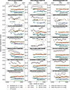 |
Fig. C.1. Optical and infrared light curves for the sources in our sample, binned in 50-day intervals. The reference modified Julian date (MJD) corresponds to the start of observations by ZTF. The number shown above each panel corresponds to the Gaia DR3 source ID. |
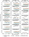 |
Fig. C.1. continued. |
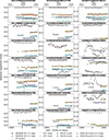 |
Fig. C.1. continued. |
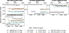 |
Fig. C.1. continued. |
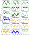 |
Fig. C.2. Folded light curves of the periodic variables in our sample. Colours represent different bands: ZTF g-band (green), ASAS-SN V-band (cyan) and g-band (blue), and ATLAS o-band (orange). The periods used to fold the light curves are shown in the bottom-left corner of each subplot. |
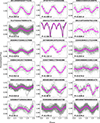 |
Fig. C.3. Same figure as Fig. C.2, but with the light curve data from TESS. Grey points represent the original unbinned data, while pink points show the data binned into 50 bins, each with a width of 0.04 in phase space. |
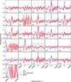 |
Fig. C.4. Flux normalised Hα velocity profiles for the subsample of observed sources (similar to Fig. 5). We compare the Gaia low-resolution BP/RP spectrum (red solid line) with our new follow-up spectrum, degraded to match the BP/RP resolution (blue dashed line). The original-resolution follow-up spectrum is plotted in grey for comparison. All sources are shown on the same scale. The index corresponding to each source (see Table B.2) is shown in the bottom left corner of each spectrum. |
All Tables
Information of the candidates in our sample: sky position, distance, apparent magnitude, colour, line-of-sight extinction, mass, surface gravity and effective temperature.
Observation date, instrument and instrument details for the follow-up spectra obtained for a subsample of our candidates.
Summary of our results, where the spectral classification and properties observed in the light curve and spectra of our candidates, together with the periods found, are reported.
All Figures
|
Fig. 1. Initial selection of our sample of mass-transferring candidates, based on a) the Gaia EDR3 StarHorse colour-magnitude diagram, b) the Gaia XP spectra, c) the AllWISE colour-colour diagram, and d) the GaiaG-band variability. In a, c, and d, we show the final sample of 67 candidates as orange stars. The red lines in a show the cuts used to select stars between the MS and the RGB based on MESA Isochrones & Stellar Tracks. In b, we show the Gaia XP spectrum of one of the sources in our sample as an example, and we compare it with our follow-up spectrum taken with CAFOS (see Section 3.2), and the ⊕ symbols represent telluric absorption (absorption by the Earth’s atmosphere). The red dashed lines in panel c indicate the zero levels and divide the plot into four regions: warm dust, hot dust, both hot and warm dust, and no hot or warm dust. The shaded green region in d corresponds to the 90th percentile of the initial HG sample. |
| In the text | |
|
Fig. 2. Overview of the selection process with the number of sources at each stage of the selection. |
| In the text | |
|
Fig. 3. Sky map showing the position of the 67 sources in our initial sample with reference to the Galactic density of stars, constructed with a Gaia DR3 random data set containing 100 000 sources. Different ranges of absolute magnitude are shown with different markers. |
| In the text | |
|
Fig. 4. Optical spectra for the subsample of spectroscopically characterised sources. Each spectrum, except for the Mookodi spectrum, is de-reddened for visualisation purposes using the best extinction values (see Sect. 6.1, Table B.1), with Fitzpatrick (1999) dust extinction function and RV = 3.1. The main emission and absorption lines are indicated. The areas with strong telluric absorption are shown by the shaded rectangles. On the right, the number in parentheses indicates the index associated with each source (see Table B.2), and this index is followed by the instrument used to take each spectrum: CAFOS (CAF) from the Calar Alto Observatory 2.2 m telescope, HERMES from the Mercator telescope, FIES and ALFOSC (ALF) from the Nordic Optical Telescope, and Mookodi from the South African Astronomical Observatory 1 m Lesedi telescope. |
| In the text | |
|
Fig. 5. Flux normalised Hα and Hβ velocity profiles for the subsample of observed sources. All sources are shown on the same scale. The index corresponding to each source (see Table B.2) is shown in the bottom left corner of each spectrum. Medium- and high-resolution spectra have been binned using 10 km s−1 bins for improved visual representation. |
| In the text | |
|
Fig. 6. Light curves of three sources in our sample illustrating the types of variability defined in this work (see Sect. 4.1.1). Circles represent the ZTF g band (green) and r band (red), while grey diamonds correspond to the NEOWISE W2 band. For clarity, the g-band and the W2-band light curves are vertically offset in all three panels, and the SR example is binned to better show its long-term evolution. The reference modified Julian date (MJD) corresponds to the start of the ZTF survey. |
| In the text | |
|
Fig. 7. Top: Pie chart with the types of periodic variables identified in our sample. Bottom: Pie chart with the spectral classes in our sample, combining the results of our classification and the classes reported in the Gaia DR3. |
| In the text | |
|
Fig. 8. Positions of the nine sources for which we re-estimated extinction (see Sect. 4.2.3) in the colour-magnitude diagram. Red squares indicate the positions derived using StarHorse, while blue diamonds show the positions computed using our extinction estimates based on diffuse interstellar bands, averaging the results from the 5780 Å and 6614 Å lines. For comparison, we also show the positions of all sources in our sample using the SHBoost catalogue (black stars; see Sect. 6.1). The schematic boxes denote the typical locations of different stellar types. |
| In the text | |
|
Fig. 9. Comparison of the observed period and the theoretical period of a binary in which one star fills its Roche lobe (see Sect. 6.3.4). Different marker shapes correspond to different types of stars, and colours represent spectral classes (using our classification when available, and Gaia’s otherwise). Sources that lie, based on SHBoost values, within our defined HG parameter space are highlighted with circles. |
| In the text | |
|
Fig. 10. Light curve (left column), phase-folded light curve (middle column), and spectrum (right column) of our two best candidates for mass-transferring merger progenitors: 6228685649971375616 (top row) and 6123873398383875456 (bottom row). For both sources, a model spectrum from the Castelli–Kurucz Atlas (Castelli et al. 2003), with Teff = 6100 K and log g = 3.75, is shown for comparison. The ZTF and NEOWISE data in the light curves (left column) are offset for visual clarity, and the reference modified Julian date (MJD) in the light curve corresponds to the start of observations by ZTF. Although we report a sinusoidal period of 0.39674 d for 6123873398383875456, the phase-folded light curve is shown using twice this period, consistent with our interpretation of the source as a contact eclipsing binary. The ⊕ symbols and shaded areas in the spectra (right column) represent telluric absorption (absorption by the Earth’s atmosphere). |
| In the text | |
|
Fig. C.1. Optical and infrared light curves for the sources in our sample, binned in 50-day intervals. The reference modified Julian date (MJD) corresponds to the start of observations by ZTF. The number shown above each panel corresponds to the Gaia DR3 source ID. |
| In the text | |
|
Fig. C.1. continued. |
| In the text | |
|
Fig. C.1. continued. |
| In the text | |
|
Fig. C.1. continued. |
| In the text | |
|
Fig. C.2. Folded light curves of the periodic variables in our sample. Colours represent different bands: ZTF g-band (green), ASAS-SN V-band (cyan) and g-band (blue), and ATLAS o-band (orange). The periods used to fold the light curves are shown in the bottom-left corner of each subplot. |
| In the text | |
|
Fig. C.3. Same figure as Fig. C.2, but with the light curve data from TESS. Grey points represent the original unbinned data, while pink points show the data binned into 50 bins, each with a width of 0.04 in phase space. |
| In the text | |
|
Fig. C.4. Flux normalised Hα velocity profiles for the subsample of observed sources (similar to Fig. 5). We compare the Gaia low-resolution BP/RP spectrum (red solid line) with our new follow-up spectrum, degraded to match the BP/RP resolution (blue dashed line). The original-resolution follow-up spectrum is plotted in grey for comparison. All sources are shown on the same scale. The index corresponding to each source (see Table B.2) is shown in the bottom left corner of each spectrum. |
| In the text | |
Current usage metrics show cumulative count of Article Views (full-text article views including HTML views, PDF and ePub downloads, according to the available data) and Abstracts Views on Vision4Press platform.
Data correspond to usage on the plateform after 2015. The current usage metrics is available 48-96 hours after online publication and is updated daily on week days.
Initial download of the metrics may take a while.