| Issue |
A&A
Volume 706, February 2026
|
|
|---|---|---|
| Article Number | A163 | |
| Number of page(s) | 20 | |
| Section | Galactic structure, stellar clusters and populations | |
| DOI | https://doi.org/10.1051/0004-6361/202557231 | |
| Published online | 11 February 2026 | |
The mysterious globular cluster population of MATLAS-2019
1
Instituto de Astrofísica de Canarias,
c/ Vía Láctea s/n,
38205
La Laguna, Tenerife,
Spain
2
Departamento de Astrofísica, Universidad de La Laguna,
38206
La Laguna, Tenerife,
Spain
3
Institute of Space Sciences (ICE, CSIC), Campus UAB,
Carrer de Can Magrans, s/n,
08193
Barcelona,
Spain
★ Corresponding author: This email address is being protected from spambots. You need JavaScript enabled to view it.
Received:
12
September
2025
Accepted:
10
December
2025
Abstract
MATLAS-2019 (also known as NGC5846-UDG1) has attracted significant attention due to the ongoing debate surrounding its globular cluster (GC) population, with several studies addressing the issue, yet reaching little consensus. For this paper, we took advantage of HST’s multi-wavelength coverage (F475W, F606W, and F814W observations) with the addition of deep u-band imaging from the Gran Telescopio Canarias (GTC), to perform the most detailed study and estimation to date of the GC population of the ultra-diffuse galaxy MATLAS-2019. The improved constraints provided by the combination of high spatial resolution and better coverage of the GC spectral energy distribution has allowed us to obtain a clean sample of GCs in this galaxy. We report a number of 33 ± 3 GCs in MATLAS-2019, supporting the previous lower estimates for this galaxy. The GC population of this galaxy is highly concentrated with ∼80% of the GCs inside the effective radius (Re) of the galaxy, and the GC half-number radius Re,GC is 0.7 × Re. Using the GC-halo mass relation, we estimate a halo mass for MATLAS-2019 of (1.14 ± 0.1) × 1011 M⊙. The GC luminosity function and the distribution of effective radii of the GCs favour a distance to the galaxy of 20.0 ± 0.9 Mpc. In agreement with previous findings, we find that the distribution of GCs is highly asymmetric even though the distribution of stars in the galaxy is symmetric. This suggests that assumptions about the symmetry of the GC distribution may be incorrect when used to calculate the number of GCs with such low statistics.
Key words: galaxies: dwarf / galaxies: formation / galaxies: individual: MATLAS-2019 / galaxies: photometry / galaxies: star clusters: general / galaxies: structure
© The Authors 2026
 Open Access article, published by EDP Sciences, under the terms of the Creative Commons Attribution License (https://creativecommons.org/licenses/by/4.0), which permits unrestricted use, distribution, and reproduction in any medium, provided the original work is properly cited.
This article is published in open access under the Subscribe to Open model. This email address is being protected from spambots. You need JavaScript enabled to view it. to support open access publication.
1 Introduction
Ultra-diffuse galaxies (UDGs) are a subset of dwarf galaxies with two identifying characteristics: a faint central surface brightness (µg(0) ≳ 24 mag arcsec−2) and a large effective radius (Re ≳ 1.5 kpc; van Dokkum et al. 2015). They have been found in a wide range of environments: clusters (e.g. Coma: van Dokkum et al. 2015, Fornax: Muñoz et al. 2015, Virgo: Lim et al. 2020, Perseus: Marleau et al. 2025), groups (e.g. Román & Trujillo 2017; Trujillo et al. 2017; Galinski & Romanowsky 2023; Fielder et al. 2024), and the field (e.g. Greco et al. 2018; Román et al. 2019; Marleau et al. 2021; Jones et al. 2023). Two main hypotheses have been proposed to explain the origin of objects with such properties. The first is that they are normal dwarf galaxies that underwent some process that ‘puffed’ them up: high initial spins (Amorisco & Loeb 2016), stellar feedback (Di Cintio et al. 2017), early mergers (Wright et al. 2021), tidal heating of dwarf galaxies (Fielder et al. 2024), effects of clusters’ tides (Sales et al. 2020), or tidal disruption (Žemaitis et al. 2023). The second hypothesis is that they were going to host a larger stellar content but were prematurely quenched and ceased to form stars. Consequently, they are now embedded in dark matter haloes that are more massive than expected given their stellar mass (van Dokkum et al. 2015, 2016; Beasley & Trujillo 2016; Toloba et al. 2018).
One way to distinguish between these formation scenarios would be to infer the mass of the dark matter halos, as it would give us valuable insights into the nature of these objects. However, using direct methods, such as stellar velocity dispersion or rotation curves, is usually not feasible for such faint systems, and indirect measurements of the masses need to be employed. For example, the number of globular clusters (GCs; NGC) appears to correlate with the total mass of the galaxy (e.g. Blakeslee et al. 1997; Spitler & Forbes 2009; Hudson et al. 2014; Harris et al. 2017; Forbes et al. 2018; Le & Cooper 2025). If this relation also holds for UDGs, then this will provide a relatively easy way to infer the amount of dark matter of these systems.
Studies of UDGs have found both rich GC systems (van Dokkum et al. 2017; Forbes et al. 2020; Müller et al. 2021; Danieli et al. 2022; Marleau et al. 2024) and systems in line with typical dwarf galaxies of the same stellar masses (Amorisco et al. 2018; Saifollahi et al. 2021; Marleau et al. 2021). But there is one particular galaxy that stands out for its abundant GC system. This object, NGC5846-UDG1 or MATLAS-2019, was identified as a very low surface brightness (VLSB) galaxy with the name NGC 5846-156 by Mahdavi et al. (2005) but later re-classified as an UDG in Forbes et al. (2019) and Poulain et al. (2021). It has an effective radius (Re) of 17.″2 (Müller et al. 2020) and its systemic velocity (2156 ± 9 km s−1, Müller et al. 2020) is consistent with the velocity of the NGC 5846 group, which suggests that it is a member of the group.
Forbes et al. (2021) estimated a number of ∼45 GCs using ground-based imaging from the VEGAS survey, which is compatible with Danieli et al. (2022), who found 54 ± 9 GCs, using high-resolution Hubble Space Telescope (HST) imaging (WFC3; F475W and F606W bands), which is more than any previously known galaxy with similar properties. In contrast, Müller et al. (2021), using another set of observations from the HST (ACS; F606W and F814W bands), found a population of 26 ± 6 using a Bayesian approach (36 ± 6 using a non-Bayesian approach), which places MATLAS-2019’s GC system in line with the systems of other UDGs. A more recent study from Marleau et al. (2024) finds, using also HST (ACS; F606W and F814W), 38 ± 7 GCs for MATLAS-2019, which is somewhere in between previous studies.
In addition to the disagreement in the number of GCs, the distance to the galaxy is still an open question. Using surface brightness fluctuations (SBF), Danieli et al. (2022) measured a distance of 21 ± 5 Mpc to MATLAS-2019 but ended up using the group’s distance due to the low signal-to-noise ratio of the measurement (i.e. 26.5 Mpc from the weighted average distance of the members from the Cosmicflows-3 catalogue; Tully et al. 2016; Kourkchi & Tully 2017; Danieli et al. 2022). On the other hand, Müller et al. (2021), using the peak of the GC luminosity function (GCLF), found a distance of  Mpc.
Mpc.
For this work, we took advantage of all of HST’s high-resolution, multi-band imaging to revise the estimation of the number of GCs of MATLAS-2019. The improved constrains provided by the high spatial resolution and better sampling of the spectral energy distribution of these objects were necessary to minimise contamination from foreground and background sources. We also used deep data from the Gran Telescopio Canarias (GTC) to refine the identification of GCs and to characterise the stellar body of this galaxy. We compare our results with previous estimates of the GC population from the literature and explore its implications for our understanding of UDG formation. Throughout this work we adopt a standard cosmological model with the following parameters: H0 = 70 km s−1 Mpc−1, Ωm = 0.3 and ΩΛ = 0.7. All magnitudes are given in the AB system unless otherwise specified.
2 Data
The data used in this paper come from two different facilities: the Hubble Space Telescope (HST) and the 10.4m Gran Telescopio Canarias (GTC). The details of the observations are described below.
2.1 Hubble Space Telescope imaging
MATLAS-2019 was observed with HST as part of two different sets of observations. One using the Advance Camera for Surveys (ACS) and the other using the Wide Field Camera 3 (WFC3). Both datasets were retrieved from the MAST archive1.
2.1.1 Advanced Camera for Surveys
The ACS images were obtained using the Wide Field Channel (WFC) as part of the programme GO-16082 (PI: Müller). The galaxy was observed in the F606W and F814W bands, although in this paper we will only use F814W. The reason for this is deeper F606W data exist taken with the WFC3. The total exposure time of the images is 1030 seconds for both bands. We used the charge-transfer efficiency (CTE) corrected images (.drc.fits files) produced by the standard pipeline.
2.1.2 Wide Field Camera 3
The images from the WFC3 were obtained using the UVIS channel as part of the programme GO-16284 (PI: Danieli). The galaxy was observed in the F475W and F606W bands, with a total exposure time of 2349 and 2360 seconds respectively. The CTE corrected images (.drc.fits files) produced by the standard pipeline are used as well.
5σ limiting depths using apertures twice the FWHM of the GC profiles for each of the images used to identify the GC candidates of MATLAS-2019.
2.2 GTC images
In order to improve our identification of GCs and study the light distribution of MATLAS-2019, we obtained deep optical and multi-band imaging with GTC, using the upgraded camera Optical System for Imaging and low-Intermediate-Resolution Integrated Spectroscopy (OSIRIS+). The galaxy was observed between the 18 and 26 of April 2023 in the u, g and r filters as part of the programme GTC57-22B (PI: Trujillo). The final exposure times on-source are 5580, 5940 and 5760 seconds, respectively. The observational strategy and data reduction of the observations are described in Appendix D.
2.3 Image depth
The aim of this work is to obtain the most accurate sample of GC candidates of MATLAS-2019. To achieve this, we first need to estimate the limiting depth of our images which characterises the magnitude to which is reasonable to trust our detections. Since we are interested in characterising the limits for detecting GCs, we compute this limiting depth on our images using apertures based on the full-width-at-half-maximum (FWHM) that the spectroscopically confirmed GCs have in the images (see Sect. 3.1). Thus, we randomly place, after masking all the sources in the images, 20 000 apertures of diameter twice the FWHM of the GC profiles in each image. That is: 0.″216 (5.4 px) for the WFC3 data, 0.″270 (5.4 px) for the ACS data, and 2.″2 (8.6 px) for the OSIRIS+ data. We calculate the resulting distributions and its 5σ values, which are listed in Table 1.
Due to the difference in resolution and depth between the HST and GTC data, HST imaging will be used to detect and select the GC candidates of this galaxy. The OSIRIS+ images will be used to characterise the stellar body of the galaxy, while the u-band will also be used to clean up the initial catalogue of GC candidates. In Table 2 details of the OSIRIS+ data are provided.
3 The globular cluster system of MATLAS-2019
The task of identifying GCs in galaxies is not trivial. Foreground and background contamination makes it difficult to characterise the overall GC system of the host galaxy with accuracy. Recent works have shown the increased effectiveness of identifying GCs using more information from their spectral energy distributions (e.g. Montes et al. 2014; Muñoz et al. 2014) to help separate them from contaminants. Müller et al. (2020) already identified 11 GCs in MATLAS-2019 using spectroscopy, and Haacke et al. (2025) further extended the sample of spectroscopically confirmed GCs to 20. Here, we aim to find objects that are similar (both in morphology and colours) to the spectroscopically confirmed GCs, taking into account sources that may have been too faint for spectroscopic follow-up or that are located outside the coverage of the spectroscopic observations. Note that the faintest spectroscopically confirmed GCs in Haacke et al. 2025 are well below 2σ from the expected GCLF, see Sect. 3.4.
Characteristics of the OSIRIS+ ultra-deep imaging of MATLAS-2019.
3.1 Characterising the light profiles of the GCs
At the distance of MATLAS-2019, the resolution of HST allows to resolve the GCs of this galaxy, i.e. objects with an effective radius of ∼3 pc. The FWHM of the point spread function (PSF) of the images (measured directly from stars both in WFC3 and ACS) is ∼2.2 px while the typical FWHM of a spectroscopically confirmed GC is ∼2.7 px (see below). Therefore, it is crucial to study the light profiles of the spectroscopically confirmed GCs in order to define the parameters needed to perform accurate photometry: aperture, aperture correction and distance from the centre of the GC to perform the local background estimation.
3.1.1 GC 1D radial profiles
Light profiles of the spectroscopically confirmed GCs are derived in sufficiently large stamps (81px × 81px), which allow us to explore the profiles until they fade away in the noise. On these stamps we measure the centroid of the objects using centroid_2dg from the photutils package (Bradley et al. 2023). We then characterise the local background in order to subtract it from the stamps. To do this, we explore different radii and widths for the background annulus, looking to minimise the root mean square (RMS) of the background region for each GC profile. The minimum RMS on the background region is found using an annulus with a width of 6 px (0.″24 in WFC3 and 0.″3 in ACS imaging) and with an inner radius of diameter 64 px (2.″56) for the WFC3, and 60 px (3.″00) for the ACS. Once we have the background subtracted stamps, we derive the radial profiles using the RadialProfile routine from photutils. We compute the average GC profile, weighting the profiles at each radius by their total fluxes (i.e. wi = Fi/Fmax). Fig. 1 shows the radial profiles for the 20 confirmed GCs from Müller et al. (2020) and Haacke et al. (2025) (grey), the S/N-weighted mean profile (blue), the region where the background is estimated (light blue region), the profile of the empirical PSF provided by STScI2 (green), and the profile of the PSF obtained directly from stars of the images (orange). All profiles are normalised to the unit at the centre. Finally, to define the limiting radius of the profiles, we truncate the profiles when they reach 5 times the value of the standard deviation of the background. To avoid any colour bias, we use the same limit for all the bands, which is the shallowest i.e. 0.″60 arcsec in F814W.
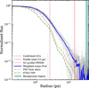 |
Fig. 1 GC radial profiles in the WFC3/F606W band for the 20 spectroscopically confirmed GCs (grey). The blue line shows the S/N weighted mean profile of the GCs. We also plot the profile of the empirical PSF provided by the STScI in green, and the profile of the PSF obtained directly from stars of the images in orange. The vertical dashed red line (0.″6, equivalent to 15 px in WFC3 imaging) indicates where the profile is truncated, the vertical dotted brown line shows the FWHM of the mean GC profile, and the light blue region indicates where the background has been estimated. |
3.1.2 PSF of the images
The PSF has been modelled in a similar way as the mean profile of the GCs (see previous section), but this time combining bright, non-saturated, and non-contaminated stars from the images. Thus, we derive the 1D radial profiles of the stars, and obtain the mean profile weighting them by their total fluxes at each radius.
In order to be more robust in our analysis of the PSF, we will take both our PSF model and the empirical PSFs provided by STScI into account (more details in Sect. 3.1.3). Thus, the PSF built with stars from the image has a FWHM of 2.2 px and the PSF given by STScI has a FWHM of 1.75 px.
3.1.3 Photometric and aperture corrections
After obtaining the weighted mean radial profile of the GCs in each of the filters, we derive the photometric apertures. We defined the apertures here to have a diameter of 2 times the FWHM of the GCs. We estimate this FWHM from the mean GC profile. The FWHM is 2.7 px, both in the WFC3 and ACS images.
We also use the GC radial profiles to derive the aperture corrections up to infinity, in order to obtain the most accurate photometry of the GCs. We divide this step into two parts – defined in terms of diameters – from 2 × FWHM to 1.″2 and from 1.″2 to infinity. The first correction, from 2 × FWHM to 1.″2, is derived from the mean GC profile as follows. We compare the amount of flux enclosed in 2 × FWHM with the amount of total flux of the profile up to 1.″2, which gives us the first correction.
For the second step, the correction to infinity, we need to extend the GC radial profile derived above, i.e. we need to estimate the slope in the outer parts of the GC profile. The slope of the outer parts of the GC profiles at large radii is assumed to be the same to that of the PSF in the outermost region. Therefore, we fit a power law to the outer parts (from 3 px to 10 px) of the empirical PSFs provided by STScI and our PSF constructed from stars in the images. The slope we use is the average of the two derived slopes, while the difference between them is included as the uncertainty of the correction. Once we have radially extended our GC profiles, we calculate the corrections to infinity. Table 3 gives the corrections for the two steps, which are applied as mcorr = mini + mcorr1 + mcorr2.
Photometric corrections based on the properties of the GCs in the images.
3.2 GC pre-selection
Once we have defined the parameters for performing photometry, we can build a preliminary catalogue of candidate GCs. As a first step, we take advantage of the high-resolution HST data to select them based on their morphology. First, we build catalogues of objects by running SExtractor (Bertin & Arnouts 1996) in the HST images3. To perform the photometry, we use the python package photutils with apertures of diameter 2 × FWHM of the confirmed GCs, estimating the background and performing the corrections described in Sect. 3.1.1 and Sect. 3.1.3. The Galactic extinction correction is applied afterwards (AF475W = 0.171, AF606W = 0.131, AF814W = 0.081)4. We match the catalogues in the three HST filters (F475W, F606W and F814W) using their sky position with a tolerance based on the typical extension of the brightest GCs of the galaxy (i.e. 0.5 arcsec).
We identify GC candidates based on their effective radius (Re), ellipticity, and magnitude in the F606W band (mF606W). This pre-selection criteria is modelled upon the properties of the confirmed GCs of MATLAS-2019 as well as local GCs (Harris 1996; Georgiev et al. 2009a). We select sources between mF606W = 19.5 mag and mF606W = 27.1 mag5. The faint limit corresponds to the 5σ limiting depth calculated in Sect. 2.3. The bright limit corresponds to the magnitude of the brightest GC from the MW and from nearby dwarfs (Harris 1996; Georgiev et al. 2009a) in the case that MATLAS-2019 is at 20.7 Mpc (this is a conservative limit, since a GC this bright would be fainter if MATLAS-2019 is at 26.5 Mpc; see Appendix F.3 for a comparison between the MW and nearby dwarfs GCs and the GCs of MATLAS-2019).
The effective radius and magnitude are taken from our deepest image (WFC3/F606W) while the ellipticity used is the average between the ellipticity from the three HST bands in order to maximise the reliability of the measurement. The ellipticity and effective radius are measured using SExtractor. To obtain an approximate value for the Re, we analytically deconvolve the FWHM of the candidate GC obtained from SExtractor with the FWHM of the PSF of the images under a Gaussian assumption. To convert to a physical size, we assume a distance of 20.7 Mpc6.
The pre-selection criteria is the following:
0 pc ≤ Re ≤ 10 pc
0 ≤ ellipticity ≤ 0.2
19.5 mag ≤ mF606W ≤ 27.1 mag
Fig. 2 shows the histograms of Re, ellipticity and mF606W of all the sources detected with SExtractor (grey), the confirmed GCs in Müller et al. (2020) and Haacke et al. (2025) (hashed red) and the GC candidates based in our preliminary selection (blue). A total of 128 objects, including the 20 spectroscopically confirmed GCs, fulfil the criteria above.
3.3 Colour-colour selection
Once we have our GC candidates, the next step is to narrow down the selection based on the colours of the GCs. Fig. 3 shows the (mF475W − mF606W)0 vs. (mF606W − mF814W)0 colour-colour diagram. The 20 spectroscopically confirmed GCs in Müller et al. (2020) and Haacke et al. (2025) are indicated as red squares. All the spectroscopically confirmed GCs but one occupy a small region in the colour-colour space. This anomalous object was already pointed out by Haacke et al. (2025) as an object with a remarkable different colour. This object has a (mF475W − mF606W)0 colour at ∼7.8σ and a (mF606W − mF814W)0 colour at ∼2.7σ from the rest of the GCs. In light of this anomaly, we assume that this object is intrinsically different from the rest of the GC system (perhaps an intragroup GC) and will not be considered as a bona fide GC for the rest of the analysis. In Appendix A we explore how the results change if we include it in the analysis.
We select objects with colours between 0.34 < (mF475W − mF606W)0 < 0.54 mag and, simultaneously, 0.26 < (mF606W − mF814W)0 < 0.55 mag (orange box). Similar to Montes et al. (2020, 2021), this selection region is based on the ±3σ around the median colours of the 20 confirmed GCs (i.e. (mF475W − mF606W)0 ∼ 0.44 and (mF606W − mF814W)0 ∼ 0.41), with σ being their colour dispersion (σ(mF475W−mF606W)0 ∼ 0.034 and σ(mF606W−mF814W)0 ∼ 0.049). The violet star in Fig. 3 shows the colour predictions using the simple stellar population models from Bruzual & Charlot (2003) based on the metallicities (![Mathematical equation: $([{\rm{Fe/H}}] = - 1.44_{ - 0.07}^{ + 0.10}dex)$](/articles/aa/full_html/2026/02/aa57231-25/aa57231-25-eq2.png) ) and ages (
) and ages ( ) of the confirmed GCs of MATLAS-2019 obtained in Müller et al. (2020). The colours of the model are:
  and
and  , in agreement with our selection region. After the colour-colour selection, only 38 potential GC candidates match our criteria.
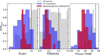 |
Fig. 2 Normalised histograms of the effective radius (in parsecs, assuming a distance of 20.7 Mpc), ellipticity and F606W magnitude of different samples of sources; N is the number of sources in each bin and Nmax the maximum of their respective histograms. The grey histogram shows all the sources of the catalogues in grey (446 sources), the red hatched histogram the 20 spectroscopically confirmed GCs and the blue histogram the sources which fulfil the selection criteria (128 sources). The vertical dashed lines indicate the ranges of the GC selection, in each of the parameters. |
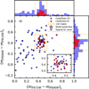 |
Fig. 3 (mF475W − mF606W)0 vs (mF606W − mF814W)0 colour-colour diagram of the initial sample of GC candidates. The 20 spectroscopically confirmed GCs (Müller et al. 2020; Haacke et al. 2025) are shown as red squares. The orange dashed box indicates the region we have selected for our next sample of GC candidates and corresponds to ±3σ around the median colours of the confirmed GCs (excluding the anomalous object, see Sect. 3.3). The violet star, and its error bar, shows the prediction from Bruzual & Charlot (2003) models for an SSP of [Fe/H] = –1.44 dex and 9.1 Gyr (Müller et al. 2020). The inset shows a zoom-in into the dashed orange box for ease of viewing. The error bars shown in the upper-left corner are the errors of an object located at the peak of the GCLF (mF606W = 23.77 mag, assuming a distance of 20.7 Mpc to the galaxy). |
OSIRIS+ u-band photometry
We take advantage of the availability of the u-band from OSIRIS+ to further refine our GC candidate sample. The u-band is especially useful to separate GCs from other sources such as foreground stars, as horizontal branch stars present in these metal-poor GCs contribute to its flux (e.g. Taylor et al. 2017). As mentioned in Sect. 2.3, this colour criterion is applied separately because of the different properties of the GTC and HST data.
The photometry in the u-band data is performed at the locations where the sources were detected in the HST images. The apertures used are based on the PSF of the OSIRIS+ image, modelled in the same way as the PSF in the HST bands (Sect. 3.1.2). Thus, the diameter used for the aperture is 2 × FWHM of the PSF (D = 2.″2 = 8.6 pix). Analogous corrections to those explained in Sect. 3.1.3 have been calculated for the u-band. Thus, we obtain that a correction of −0.4 mag is needed for the first step (from the aperture to the end of the profile), and a second correction of −0.04 mag when extrapolating to infinity. Again, these are applied as mcorr = mini + mcorr1 + mcorr2. Afterwards, the photometry has also been corrected from extinction (Au = 0.269 mag).
Fig. 4 shows the same colour-colour diagram as in Fig. 3, but in this case the GC candidates are colour-coded by the (mu − mF475W)0 colour. We obtain a median (mu − mF475W)0 colour of 1.20 mag and a standard deviation of 0.15 mag for the spectroscopically confirmed GCs. The expected (mu − mF475W)0 colour based on the properties of the spectroscopically confirmed GCs and on the Bruzual & Charlot (2003) models is  . We select those objects within a range of ±3σ (i.e. 0.75 < (mu − mF475W)0 < 1.65). Note that we can only apply this selection to objects that are observed in the u-band, i.e. mu < 25.8 mag (see Appendix B). Applying this colour selection, we end up with 35 GC candidates. We highlight the GCs rejected by including the u-band in Fig. 4. Fig. 5 shows the distribution of the (mu − mF475W)0 colours for the candidates and for the spectroscopically confirmed GCs.
To summarise, the colour ranges used in this work are:
0.34 mag < (mF475W − mF606W)0 < 0.54 mag
0.26 mag < (mF606W − mF814W)0 < 0.55 mag
0.75 mag < (mu − mF475W)0 < 1.65 mag.
The coordinates and parameters measured of all the objects are compiled in Table C.1 and Fig. 6 shows a smoothed WFC3/F606W MATLAS-2019 image with the GC candidates marked as open blue circles.
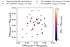 |
Fig. 4 (mF475W −mF606W)0 vs (mF606W −mF814W)0 colour-colour diagram of GC candidates, colour-coded with the (mu − mF475W)0 colour. The 20 spectroscopically confirmed GCs (Müller et al. 2020; Haacke et al. 2025) are shown as squares and the candidates as circles. The size of the marker indicates the mF606W of the source, as shown in the legend. The sources in grey are objects that are too faint to be measured in the u-band. The blue open circles highlight those objects rejected based on their (mu − mF475W)0 colour. |
 |
Fig. 5 Normalised histograms of the (mu − mF475W)0 colour of the GCs of MATLAS2019; N is the number of sources in each bin and Nmax the maximum of their respective histograms. The red hatched histogram shows the spectroscopically confirmed GCs and the blue histogram the GC candidates. Only sources with trustable magnitude in the u−band are shown (i.e. mu < 25.8, see Sect. 3.3). The dashed vertical black lines indicate the ±3σ cut applied for GC selection. |
3.4 Final number of GC candidates
Errors in photometry, ellipticity, and Re could affect our identification of GCs. To determine the completeness and characterise the errors on the photometry and the morphological parameters derived above, we perform a series of tests by injecting artificial GCs on the images. Further details on these tests are given in Appendix B.
We use the results of these tests to assess how the errors in colour, magnitude, ellipticity, and effective radius impact the selection of GC candidates. To do so, we performed 10 000 realisations where the parameters of the detected sources (i.e. detections matched among the three HST filters, excluding the spectroscopically confirmed GCs) have been perturbed by drawing a value from the distribution of their errors, assuming a Gaussian distribution. The aim is to statistically characterise the identification of GC candidates of MATLAS-2019 based on the previously described procedure. For each of these realisations, we derive a candidate GC sample. The median number of detected GCs is 32, with a standard deviation of 3. Consequently, although we identify 35 sources as GC candidates, the expected population of GCs of the galaxy is 32 ± 3.
We also estimate how many GCs might be missing due to the limited depth of our images. In dwarf galaxies, the GC luminosity function (GCLF) peaks around MV(Vega) = −7.3 with a width of σ ∼ 1 (e.g. Miller & Lotz 2007), although other studies suggest narrower distribution σ ∼ 0.6 (e.g. Carlsten et al. 2022). Thus, the expected GCLF would peak at mF606W(AB) = 24.13 mag7 if the galaxy is at 20.7 Mpc or mF606W(AB) = 24.67 mag if it is at 26.5 Mpc. Being conservative and assuming a wider GCLF in dwarfs (i.e. 1 mag), the 2σ value from the peak will be located at mF606W = 26.13 mag at 20.7 Mpc or mF606W = 26.67 mag at 26.5 Mpc. Based on completeness tests (Appendix B), we reach 90% completeness in WFC3/F606W around 26.5 mag, this means that we are only missing ∼2.5% of the sources, regardless of the assumed distance. This adds 1 GC to our statistical estimation.
All in all, we end up with a population of 35 GCs for MATLAS-2019. After characterising and exploring the errors in the selection parameters, the expected number of GCs ends up being 32 ± 3 objects. Including the completeness correction due to the depth of our images, the final population is 33 ± 3.
3.5 Contamination
Due to the slightly different fields covered by the different images used in this work, it is not straightforward to define a control field for assessing the contamination. We have estimated it by assuming as our control field the region outside 2Re (Re = 17.″2, Müller et al. 2020) of the galaxy (being conservative with respect to Müller et al. 2021, where it is found that the GC radial distribution falls to background levels beyond 1.75Re), where 4 candidates are found. Doing this, we find that the contamination level in our sample is ∼1 GC. As expected – due to the exhaustive morphological and colour criteria – the contamination is low. Moreover, two of the four candidates that lie outside 2Re have GC-like profiles, in contradiction with what we would expect from contaminants. Thus, we judge sensible to be conservative and not to consider these objects as interlopers in spite of their far location to the centre of MATLAS-2019.
Fig. 7 shows the radial profiles for the GC candidates in this work. The confirmed GCs from Müller et al. (2020) and Haacke et al. (2025) are in black, the new candidates identified in this work in grey, and the PSF is shown as the dashed green line. The candidates located >2Re from the centre of MATLAS-2019 are shown in red. Two of them have profiles that are similar to the profiles of confirmed GCs, suggesting that they are likely GCs. On the other hand, two of them deviate from the general trend and resemble a point source. These point-like sources are strong interlopers candidates, but we have not discarded them as more information is needed. In Table C.1 these candidates are flagged, along with another GC candidate with also a point-like profile.
4 Stellar properties of MATLAS-2019
The ultra-deep imaging of MATLAS-2019 with OSIRIS+ allows us to assess its optical morphology in detail for the first time, as previous imaging (e.g. Forbes et al. 2020; Habas et al. 2020; Müller et al. 2021; Danieli et al. 2022) was not deep enough to reveal the low surface brightness features of the galaxy (i.e. mainly tidal features or asymmetries in the outskirts). The outer parts of low-mass galaxies, such as MATLAS-2019, can provide direct evidence for their hierarchical merging assembly. For example, asymmetries or other perturbations indicate tidal interactions with nearby galaxies (Johnston et al. 2002; Montes et al. 2020; Golini et al. 2024). In this section, we explore the deep images from OSIRIS+ to gain a deeper understanding of the physical processes that this galaxy may have undergone.
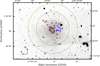 |
Fig. 6 HST WFC3/F606W image convolved with a Gaussian kernel (σ = 1.5) showing the spatial distribution of the GC candidates identified in this work. The red circles indicate the GCs spectroscopically confirmed in Müller et al. (2020) and Haacke et al. (2025) while the blue circles highlight the GCs candidates and the orange circle represent the anomalous GC. The yellow dashed circles indicate 1Re, 2Re and 3Re of the galaxy (Re = 17.″2, Müller et al. 2020). |
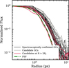 |
Fig. 7 Comparison of radial profiles in the WFC3/F606W band. We show the profiles of the spectroscopically confirmed GCs, the GC candidates obtained in this study in grey, the profile of the PSF from stars in green, and the profiles of 4 candidates located at more that 2Re from the galaxy’s centre in red. |
4.1 Surface brightness radial profiles
Signs of interactions will show up in the radial surface brightness profiles as an excess of light at large radii and deviations from the morphology of the inner parts of the galaxy (see e.g. Johnston et al. 2002). To derive the surface brightness profiles of MATLAS-2019 we follow the steps below.
We run SExtractor in a deep combined g + r image and obtain the segmentation map to mask background and foreground sources. This mask was visually inspected to manually mask any remaining light that was missed by SExtractor. Once all sources of contamination are masked out, we run ellipse (Jedrzejewski 1987) in photutils (Bradley et al. 2023) leaving all the parameters free to derive the radial profiles of the galaxy’s ellipticity and position angle (PA).
The right panel of Fig. 8 shows the PA (top) and ellipticity (bottom) radial profiles of MATLAS-2019. In the inner parts of the galaxy (R < 30″) we see a large scatter in PA and ellipticity due to the conservative masking caused by the presence of bright GCs. In the outer parts, however, both ellipticity and PA appear to be constant, indicating that the galaxy is quite symmetrical (see Fig. D.2). The median values are PA = 10.◦5, and b/a = 0.07, at R > 30″. We also obtained the centre of the galaxy (RA=15h05m20.17s, Dec= +1d48m44.91s), from the output of ellipse.
To derive the radial profiles of MATLAS-2019, in the u, g and r bands, we use a similar approach as in Montes et al. (2021). We extracted the radial profiles in elliptical bins at different radial distances from the centre of the galaxy, fixing the ellipticity and PA of the bin to the average values obtained above. We used a custom python code to derive the profiles. For each of the radial bins, the intensity was obtained as the 3σ-clipped median of the pixel values. The errors are calculated as a combination of the Poisson noise in each annulus and the error given by the distribution of background pixels in each image. The profiles are corrected for the extinction of the Galaxy (E(B-V) = 0.046, see also Sect. 3.2). The left panel of Fig. 8 shows the surface brightness profiles of MATLAS-2019 in the u (blue), g (teal) and r (red) bands. From the light profiles we derive an effective radius of Re = 16.″0 ± 0.5, compatible with the value given by Müller et al. (2020) (17.″2 ± 0.2).
4.2 Colour and stellar mass density profiles
Once we derived the surface brightness profiles, we can study the radial variations of the galaxy’s stellar populations. These profiles are used to derive the (g−r)0 colour profile of the galaxy, shown in the top panel of Fig. 9. The (g−r)0 profile appears quite flat, with an average colour of ∼0.64 down to R< 30″. For R > 30″, the colour raises slightly up to a value of ∼0.7. These ’u-shape’ profiles have been found very often in previous works as indicative of the end of in situ star formation (see e.g. Azzollini et al. 2008; Bakos et al. 2008).
The bottom panel in Fig. 9 shows the stellar mass surface density of MATLAS-2019. This profile was derived using the prescriptions given in Bakos et al. (2008) that linked the surface brightness profiles in the g-band to radial variation of the mass-to-light ratio. The mass-to-light ratio was obtained from Roediger & Courteau (2015), assuming a Chabrier (2003) IMF and using the (g − r)0 colour profile of the galaxy.
From the stellar mass surface density profile, we derived the total stellar mass of MATLAS-2019 from the mass density profile, assuming circular symmetry, is  at a distance of
  (Müller et al. 2021), or 1.5 ± 0.2 × 10⁸ M⊙ if the galaxy is located at 26.5 ± 0.8 Mpc (Danieli et al. 2022).
The stellar mass surface density profile of MATLAS-2019 shows an exponential decrease up to ∼33″, corresponding to 3.3 (4.2) kpc assuming a distance of 20.7 (26.5) Mpc to the galaxy.
At this radius there is a change in the slope, or break, of the density profile that coincides with a change in the colour profile of the galaxy. This radius also coincides with the visual extension of the galaxy (see Fig. D.2). This break is similar to those found for dwarfs of the same stellar mass in Chamba et al. (2022), occurring at a similar stellar mass density (Σ∗ ∼ 0.5 M⊙/pc2). The presence of this truncation signals the edge of the galaxy, beyond which the galaxy could not reach the critical gas density threshold for star formation (Trujillo et al. 2020).
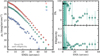 |
Fig. 8 Surface brightness, ellipticity, and PA radial profiles of MATLAS-2019. The left panel shows the u-band (blue), g-band (teal) and r-band (red) surface brightness profiles as a function of the semi-major axis obtained with a fixed centre and ellipticity (ϵ = 0.07). The surface brightness profiles have been corrected from extinction. The right panel shows the position angle (top) and ellipticity (bottom) profiles from letting the parameters of the fit vary freely. |
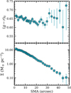 |
Fig. 9 Upper panel: OSIRIS+ colour (g − r)0 radial profile of MATLAS-2019. Bottom panel: the surface stellar mass density profile of MATLAS-2019. The density profile shows a break around ∼33″, coinciding with a change in the colour profile. |
5 Discussion
In this paper, we undertake a comprehensive identification of GC candidates for MATLAS-2019, in order to shed light on the current disagreement about this GC population. The candidates have been identified using photometry obtained from archival HST and GTC deep data, and the stellar properties of the galaxy have also been analysed. Here we discuss the implications of the GC counts found in this galaxy and how they relate to the current debate.
5.1 Comparison with previous studies
There is disagreement about the total number of GCs present in MATLAS-2019. Forbes et al. (2021) estimated a total of ∼45 GCs in this galaxy, based on Forbes et al. (2019) where about 20 compact sources were identified within 2Re of the galaxy in ground-based broadband imaging, and assuming a typical GCLF to correct for completeness. Given the differences in the datasets, mainly resolution, we cannot compare with their results.
Müller et al. (2021) used HST data to estimate a total number of GCs for MATLAS-2019 of 26 ± 6 GCs. They used a threshold in source radius, ellipticity, and (mF606W − mF814W)0 colour range finding an initial sample of 49 GC candidates within 1.75Re, which is narrowed down to 26 ± 6 using Bayesian considerations. They also estimated the population inside 1.75Re by taking into account the expected contamination in a reference background field, resulting in a population of 36 ± 6. We find that our estimate for the total population of GCs (33 ± 3) is compatible with both estimations. By using three filters information and limiting the Re of the sources, our uncertainty estimates are lower than in Müller et al. (2021) (±6 vs ±3). If we only use the same filters (F606W and F814W) but with our selection criteria, we find a population of 34 ± 2 inside 1.75Re, which is still consistent with their results in the same region and with the same filters.
Danieli et al. (2022) also used HST data to explore the GC population of MATLAS-2019. In their case, they found a total 54 ± 9 GCs (50.4 within 2Re, before completeness corrections). This would imply that MATLAS-2019 is one of the UDGs with the richest GC system. Danieli et al. (2022) selection is based in the FWHM and colour criteria from the spectroscopically confirmed GCs of the galaxy, similar to this work. However, the results are not compatible. Using only the same filters as Danieli et al. (2022) (F606W and F475W), but applying our criteria, we find 31 ± 2 candidates within 2Re, as opposed to the 50.4 GCs they find in the same area.
Danieli et al. (2022) do not apply any morphology criteria when the GC candidates have magnitudes between mF606W = 25 mag and mF606W = 26.5, which might contribute to the difference in GC numbers that we find. Nevertheless, the main difference between both studies is the range of colours used. Danieli et al. (2022) uses different colour criteria depending on the magnitude of the source, with colour bin widths ranging from 0.4 mag to 0.72 mag. On the other hand, we use a colour range of ∼0.2 mag for (mF475W − mF606W)0 and of ∼0.3 for (mF606W − mF814W)0 (which is ±3σ the median colour of the confirmed GCs). Defining the acceptance region is reaching a compromise between the accepted contamination level and the ability to correctly identify the properties of the faintest sources. Based on the photometric errors of the data (see Appendix B) and on the expected GCLF, the faintest analysed objects will have mF606W ∼ 26.5. This implies that the magnitude errors for the faintest candidates are around 0.15 mag. We consider that a selection region of around two times this value is reasonable enough and will minimise contaminants. Nevertheless, as a sanity check, applying a wider colour range (e.g. 0.2 < (mF475W − mF606W)0 < 0.8), we obtain 43 ± 2 GCs inside 2Re, more in line with Danieli et al. (2022). Our narrower colour range, combined with the addition of two extra bands and taking into account the ellipticity of the objects to separate the GCs from background sources, produces the difference.
A recent study of the GC system of MATLAS-2019 (Marleau et al. 2024), estimated a population of 38 ± 7 GCs. The data used in this study combined the data used by Müller et al. (2021) with an extra set of observations (GO-16257 and GO-16711; PI: Marleau) taken with the same instrument and filters (HST/ACS, filters F606W and F814W). The parameters used to select candidates were colour, ellipticity, Re and concentration index. Our result is lower but compatible with Marleau et al. (2024). As in the case of Danieli et al. (2022), the higher number of GCs is mainly due to the colour range accepted. Our selection window in (mF606W − mF814W)0 is narrower (being from 0.5 to 1.2 in Marleau et al. 2024), but also we filter GCs using two extra colours, (mF475W − mF606W)0 and (mu − mF475W)0, which allows us to further reject contaminants in our sample. Note that, even though we do not explicitly use the concentration index in this work, we are including that information when we analyse the light profiles of the candidates.
The fraction of light which corresponds to the GCs in MATLAS-2019 in our study is roughly 5.4 ± 0.5% (V-band, assuming MV(Vega) = −7.668 for each globular cluster and MV(AB) = −14.6 mag for the galaxy from Danieli et al. 20229), in contrast to the larger contribution (12.9% ± 0.6% in the V-band) proposed by Danieli et al. (2022). As expected in an UDG, the fraction found here is larger than the ratios of normal galaxies (e.g,. MW has ∼0.1%, assuming 160 GC and MV = −20.9, van den Bergh 1999) but in line with other UDGs and dwarfs (e.g. Forbes et al. 2020). From the results obtained in this work, the specific frequency of MATLAS-2019 (defined as  ), is 78 ± 21 (using MV = −14.1 ± 0.2 mag from Müller et al. 2021). This value is consistent with those reported in Müller et al. (2021) and Marleau et al. (2024) (59 ± 14 and 90.97 ± 16.49, respectively).
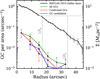 |
Fig. 10 Radial distribution of GC candidates in MATLAS-2019. The red profile represents the spectroscopically confirmed GCs, the GC candidates obtained in this study are in blue, and the whole GC system in green. The black line is the mass density profile of MATLAS-2019, as indicated in the right Y-axis. The errors in the GC profiles are the Poissonian error of the number of GCs per area in each annulus (i.e. |

5.2 Spatial distribution of the GCs
In this section, we discuss the spatial distribution of the GCs in MATLAS-2019 in order to obtain clues about the nature of this galaxy. Note that while we statistically estimate a population of 33 ± 3 (Sect. 3.4), the actual number of GCs that we identify is 35. Since based on the statistical analysis we cannot identify which specific sources are interlopers, we will use the 35 identified candidates for the study of the spatial distribution of the GC system.
Fig. 6 shows that most of the identified GC candidates are inside 1Re (26; i.e. around 80% of the total GC number) and 2Re (31), while 4 candidates are beyond 2 Re (Re = 17.″2, Müller et al. 2020). To measure the number density profile of the GC candidates, we measure the number of GCs in a set of annuli up to 45″ (about 2.5Re of the galaxy). The width of the annuli is fixed at 6″, which is about  . The resulting profiles for the different samples (confirmed in red, candidates in blue, and the whole GC system in green) are shown in Fig. 10. For comparison, we also show the stellar mass density profile of MATLAS-2019 in black. To convert GC density (in arcsec) to mass density (in pc) we assume a mass of 105 M⊙ for each GC and a distance of 20.7 Mpc (Müller et al. 2021) to MATLAS-2019. Notably, there is a lack of GC candidates towards the centre of the galaxy. This is because there are more bright GCs in this region, that can be more easily observed with spectroscopy, and the spectroscopic coverage is also better.
The GC half-number radius (i.e. the radius containing half of the GCs, Re,GC) is 12.0±0.1 arcsec. Comparing these values with the Re of the galaxy (17.″2), we find a ratio of Re,GC/Re = 0.7. This indicates that the GC system is less extended than the stellar light component of the galaxy, also seen in Fig. 10. This ratio is remarkably smaller from what other authors have claimed for other UDGs and dwarf galaxies (e.g. Janssens et al. 2024) and in line with other works (e.g. Amorisco et al. 2018; Saifollahi et al. 2022, 2025).
In addition to the spatial distribution of GC candidates, we must also consider their apparent asymmetry (see also Marleau et al. 2024). While there is a large number of candidates in the north-west of the galaxy (upper-right of the image, Fig. 6), the light distribution of the galaxy is symmetrical (Fig. D.2 and Sect. 4.1). This issue is addressed in Appendix E, concluding that we cannot rule out that the intriguing distribution of GCs in this galaxy is mere coincidence. Nonetheless, this highlights the importance of analysing the imaging before performing spatial completeness corrections, which implicitly assume symmetry for the GC system. As MATLAS-2019 shows, these assumptions might not stand and lead to the incorrect estimation of the number of GCs.
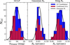 |
Fig. 11 Left panel: globular cluster luminosity function of MATLAS-2019. Middle panel: distribution of Re assuming that the intrinsic shape of the GC is a Gaussian. Right panel: distribution of Re assuming that the intrinsic shape of the GC is a King model. The spectroscopically confirmed GCs from Müller et al. (2020) and Haacke et al. (2025) are indicated in red (hatched), the population identified in this study is in blue. The widths of the bins have been calculated using the Freedman–Diaconis rule (Freedman & Diaconis 1981). The black solid line shows a Gaussian fit to the data. |
5.3 The distance to MATLAS-2019
In addition to disagreeing on the number of GCs, different studies also assume different distances to MATLAS-2019. The UDG is located in the field-of-view (FOV) of the NGC5846 galaxy group, at a projected distance of ∼21′ from NGC5846. Given the apparent consistency of the galaxy’s velocity with the group (Müller et al. 2020; Haacke et al. 2025), this strongly suggests that the distance to MATLAS-2019 is the same as to NGC5846 (i.e. 26.5 ± 0.8 Mpc from the weighted average distance of the members from Cosmicflows-3 catalogue; Tully et al. 2016; Kourkchi & Tully 2017; Danieli et al. 2022). However, Müller et al. (2021), using the GC luminosity function of the GCs (GCLF), finds that MATLAS-2019 is closer, located at  Mpc.
Mpc.
The peak of the GCLF is generally assumed to be universal and, therefore, it has been used extensively to determine distances to galaxies (Rejkuba 2012). Similarly, the Re distribution of local GCs follow an – apparently – universal Gaussian distribution, with no correlation between magnitude and Re. Thus, similar to Trujillo et al. (2019), using the GCLF and the distribution of Re we can obtain two independent distance estimates to MATLAS-2019.
In order to use the Re of the GCs as a distance indicator, we need to accurately estimate the intrinsic Re of the GCs, as it is affected (broadened) by the PSF of the images. Although we already estimated their intrinsic Re based on the FWHM measurement from SExtractor (see Sect. 3.2), we improve these measurements to provide a robust estimate of the distance. To do this, we explored both a Gaussian and a King (King 1962) model as the intrinsic shapes of a GC, and we use both values below. Further details on the measurement of the Re are given in Appendix F.1.
The GCLF and the distribution of Re of the GC candidates are shown in Fig. 11. The candidates that appear to be point-like sources (see Sect. 3.5) have not been included because they are likely interlopers and might bias our distance estimation, thus remaining a total of 32 GCs candidates. The hatched red histogram corresponds to the spectroscopically confirmed GCs from Müller et al. (2020) and Haacke et al. (2025), while the blue histogram corresponds to the GC candidates in this study. The black line indicates a Gaussian fit to the combined distributions. For the GCLF, we find that the peak is at mF606W = 23.92 mag with a σ = 0.88. Regarding the Re distribution, the peak is located at 0.″0348 when fitting a Gaussian model and 0.″0343 for the King model, with standard deviations of 0.″0115 and 0.″0170, respectively. It is noteworthy that the peaks of the distributions are the same within errors, showing that using these values to infer the distance to the galaxy is robust regardless of the assumed intrinsic profile. The slightly higher dispersion of the King model is likely due to the higher number of free parameters to be fit. The Re values used for the distributions and for measuring the distance have been circularised10.
In the literature, there are different estimations of the magnitude of the GCLF peak and the Re peak, depending on different factors such as the galaxy type and the metallicities of the GCs. We calculate the distance to MATLAS-2019 using different estimates for both the GCLF and Re peaks of the distribution, which are listed in the Appendix F.2. Fig. 12 presents the different distance estimates that are obtained for the different GCLF and Re calibrations explored. The left panel shows the distances assuming a Gaussian model as the intrinsic GC profile, while the right panel assumes a King model. For comparison, the distance obtained by Müller et al. (2021) (brown) and that obtained (grey) and assumed (pink) by Danieli et al. (2022) are shown in a black box at the bottom. We estimated a weighted mean distance of 19.9 ± 0.8 Mpc, assuming a Gaussian model for the GCs and 20.1 ± 0.8 Mpc assuming a King model, resulting in an average distance to MATLAS-2019 of 20.0 ± 0.9 Mpc. This distance implies a stellar mass for MATLAS-2019 of  .
.
The distance derived in this work is in agreement with the  Mpc obtained in Müller et al. (2021) using the GCLF and with the 21 ± 5 Mpc by Danieli et al. (2022) using surface brightness fluctuations. However, our estimated distance is not in agreement with the distance to the NGC 5846 group of galaxies (26.5 ± 0.8). Nonetheless, the galaxies in the group have estimated distances ranging from 22.7 Mpc (NGC 5839) to 34.5 Mpc (NGC 5838) (Kourkchi & Tully 2017). Therefore, MATLAS-2019 could be marginally associated to the group even though the estimated distance puts the galaxy well beyond its virial radius (0.6 Mpc, Kourkchi & Tully 2017).
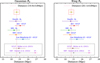 |
Fig. 12 Distance to MATLAS-2019. The left panel shows the different estimates where the Re,GC is obtained assuming that the GC intrinsic profile follows a Gaussian model, while the right panel assumes a King model. Each of the points shows a different method or calibration used to estimate the distance to MATLAS-2019 as labelled. The grey box separates the distances obtained in Müller et al. (2021) and in Danieli et al. (2022). The (*) indicates the distance assumed in Danieli et al. (2022) based on the distance to the NGC5846 group. In the red box, we plot the weighted mean distance obtained using the different estimates for the GCLF and Re,GC methods. |
5.4 The halo mass of MATLAS-2019
The number of GCs of a galaxy is closely linked to its halo mass, providing us a way to estimate the mass of its dark matter halo. This GC-Halo mass relation has been proposed to hold for a wide range of halo masses, from ∼109M⊙ to ∼1014 M⊙ (Forbes et al. 2018). Different authors have calibrated this GC-Halo mass relationship. For example, Harris et al. (2017) determined a constant ratio between the mass in the GC system and the total halo mass of MGCs/Mh = 2.9 × 10⁻⁵. If we assume a mean GC mass of 1.0 × 10⁵ M⊙ (Harris et al. 2017), we obtain a total mass in the GC system of (33 ± 3)×105 M⊙, and a halo mass of (1.14 ± 0.1) × 1011 M⊙. This estimation is consistent with Müller et al. (2021) and Marleau et al. (2024) ((0.9 ± 0.2) × 1011 M⊙ and  respectively). The number of GCs and halo mass derived here for MATLAS-2019 are in line with those of other UDGs (e.g. Beasley & Trujillo 2016; Beasley et al. 2016; Amorisco et al. 2018; Saifollahi et al. 2022; Mihos et al. 2025).
Consequently, MATLAS-2019 does not seem to inhabit an unexpectedly massive halo, in line with the halo masses expected for a dwarf galaxy (up to ∼1010−11 M⊙). However, for the halo mass we derive here, we would expect a stellar mass of ∼109 M⊙ (e.g. Girelli et al. 2020) rather than what we find ( ). This lower-than-expected stellar masses are observed in other UDGs, indicating rapid star formation quenching after the formation of the GC systems of these galaxies, as suggested in Beasley & Trujillo (2016).
6 Conclusions
MATLAS-2019 is an UDG with an unusually large GC population. There is an ongoing debate about how large this population is, where previous estimations of its GC system range from less than 30 up to more than 50 GCs. In this work, we use the multi-wavelength capabilities and high spatial resolution of archival HST data, and deep GTC data to provide a clean sample of GC candidates of this galaxy. Additionally, we explore the stellar body of the galaxy, comparing it with the distribution of GCs. Finally, we do a careful analysis of the distance to the galaxy.
We find that the GC population of MATLAS-2019 is 33 ± 3 GCs, which implies a halo mass of (1.14 ± 0.1) × 1011 M⊙. This result is in agreement with the previous lower estimates of the GC system of the galaxy (Müller et al. 2021; Marleau et al. 2024). Nevertheless, these values are larger than expected for a galaxy of the stellar mass of MATLAS-2019 ( at a distance of
  Mpc or, alternatively, M∗ = 1.5±0.2 × 10⁸ M⊙ at 26.5 ± 0.8 Mpc). This discrepancy suggests that the galaxy may have undergone rapid quenching of the stellar body of the galaxy after the bulk of GC formation.
We also confirm the previously reported asymmetry in the distribution of GCs, with a clear over-density towards the northwestern region of the galaxy. Interestingly, there is no trace of asymmetry in the body of the host galaxy. After performing a statistical analysis, we conclude that this GC asymmetry is not significant, being it compatible with a random distribution of the GC system. Additionally, the GC system appears to be highly concentrated on top of the galaxy, having 80% of the GCs inside one effective radius. Thus, the stellar light component of the galaxy is more extended that its GC system, having a Re,GC/Re of 0.7. Finally, we also estimate a distance of 20.0 ± 0.9 Mpc to MATLAS-2019 based on the peak of the GCLF and peak of the distribution of the effective radius of the GCs.
This work emphasises the necessity of using multi-wavelength and high spatial resolution data to minimise foreground and background contamination in the GC systems of UDGs. We also warn against assuming symmetry in the distribution of GCs when making spatial or coverage corrections to infer the number of GCs of these low mass systems.
Acknowledgements
We thank the referee for the constructive comments that helped improve the quality of the manuscript. We thank F. Marleau for providing the GC data of MATLAS2019 from Marleau et al. (2024). Also thank Lydia Haacke and Duncan A. Forbes for letting us compare with their data prior to publication (Haacke et al. 2025). SGA acknowledges support from grant PID2022-140869NB-I00 from the Spanish Ministry of Science and Innovation. MM acknowledges support from the project PCI2021-122072-2B, financed by MICIN/AEI/10.13039/501100011033, and the European Union “NextGenerationEU”/RTRP, from grant RYC2022-036949-I financed by the MICIU/AEI/10.13039/501100011033 and by ESF+ and program Unidad de Exce-lencia María de Maeztu CEX2020-001058-M. G.G. acknowledges support from IAC project P/302304 and through the PID2022-140869NB-I00 grant from the Spanish Ministry of Science and Innovation which is partially supported through the state budget and the regional budget of the Consejería de Economía, Industria, Comercio y Conocimientoof the Canary Islands Autonomous Community. IT acknowledges support from the State Research Agency (AEI-MCINN) of the Spanish Ministry of Science and Innovation under the grant PID2022-140869NB-I00, financed by the Ministry of Science and Innovation, through the State Budget and by the Canary Islands Department of Economy, Knowledge, and Employment, through the Regional Budget of the Autonomous Community. This research also acknowledge support from the European Union through the following grants: “UNDARK” and “Excellence in Galaxies – Twinning the IAC” of the EU Horizon Europe Widening Actions programmes (project numbers 101159929 and 101158446). Funding for this work/research was provided by the European Union (MSCA EDUCADO, GA 101119830). Views and opinions expressed are however those of the author(s) only and do not necessarily reflect those of the European Union or European Research Executive Agency (REA). MM, GG and IT acknowledge support from IAC project P/302302. This work makes use of the following code: astropy (Astropy Collaboration 2022), Source Extractor (Bertin & Arnouts 1996), Gnuastro (Akhlaghi & Ichikawa 2015), photutils (Bradley et al. 2023), numpy (Harris et al. 2020), scipy (Virtanen et al. 2020), Imfit (Erwin 2015).
References
- Abdurro’uf, Accetta, K., Aerts, C., et al. 2022, ApJS, 259, 35 [NASA ADS] [CrossRef] [Google Scholar]
- Akhlaghi, M. 2018, Gnuastro: GNU Astronomy Utilities, Astrophysics Source Code Library [record ascl:1801.009] [Google Scholar]
- Akhlaghi, M., & Ichikawa, T. 2015, ApJS, 220, 1 [Google Scholar]
- Amorisco, N. C., & Loeb, A. 2016, MNRAS, 459, L51 [NASA ADS] [CrossRef] [Google Scholar]
- Amorisco, N. C., Monachesi, A., Agnello, A., & White, S. D. M. 2018, MNRAS, 475, 4235 [NASA ADS] [CrossRef] [Google Scholar]
- Astropy Collaboration (Price-Whelan, A. M., et al.) 2022, ApJ, 935, 167 [NASA ADS] [CrossRef] [Google Scholar]
- Azzollini, R., Trujillo, I., & Beckman, J. E. 2008, ApJ, 679, L69 [NASA ADS] [CrossRef] [Google Scholar]
- Bakos, J., Trujillo, I., & Pohlen, M. 2008, ApJ, 683, L103 [NASA ADS] [CrossRef] [Google Scholar]
- Barmby, P., McLaughlin, D. E., Harris, W. E., Harris, G. L. H., & Forbes, D. A. 2007, AJ, 133, 2764 [Google Scholar]
- Beasley, M. A., & Trujillo, I. 2016, ApJ, 830, 23 [CrossRef] [Google Scholar]
- Beasley, M. A., Romanowsky, A. J., Pota, V., et al. 2016, ApJ, 819, L20 [NASA ADS] [CrossRef] [Google Scholar]
- Bertin, E. 2006, in Astronomical Society of the Pacific Conference Series, 351, Astronomical Data Analysis Software and Systems XV, eds. C. Gabriel, C. Arviset, D. Ponz, & S. Enrique, 112 [Google Scholar]
- Bertin, E. 2010, Astrophysics Source Code Library [record ascl:1010.068] [Google Scholar]
- Bertin, E., & Arnouts, S. 1996, A&AS, 117, 393 [Google Scholar]
- Blakeslee, J. P., Tonry, J. L., & Metzger, M. R. 1997, AJ, 114, 482 [Google Scholar]
- Blanton, M. R., & Roweis, S. 2007, AJ, 133, 734 [NASA ADS] [CrossRef] [Google Scholar]
- Bradley, L., Sipőcz, B., Robitaille, T., et al. 2023, https://doi.org/10.5281/zenodo.7946442 [Google Scholar]
- Bruzual, G., & Charlot, S. 2003, MNRAS, 344, 1000 [NASA ADS] [CrossRef] [Google Scholar]
- Carlsten, S. G., Greene, J. E., Beaton, R. L., & Greco, J. P. 2022, ApJ, 927, 44 [NASA ADS] [CrossRef] [Google Scholar]
- Chabrier, G. 2003, ApJ, 586, L133 [NASA ADS] [CrossRef] [Google Scholar]
- Chamba, N., Trujillo, I., & Knapen, J. H. 2022, A&A, 667, A87 [NASA ADS] [CrossRef] [EDP Sciences] [Google Scholar]
- Chambers, K. C., Magnier, E. A., Metcalfe, N., et al. 2016, arXiv e-prints [arXiv:1612.05560] [Google Scholar]
- Danieli, S., van Dokkum, P., Trujillo-Gomez, S., et al. 2022, ApJ, 927, L28 [NASA ADS] [CrossRef] [Google Scholar]
- Dey, A., Schlegel, D. J., Lang, D., et al. 2019, AJ, 157, 168 [Google Scholar]
- Di Cintio, A., Brook, C. B., Dutton, A. A., et al. 2017, MNRAS, 466, L1 [NASA ADS] [CrossRef] [Google Scholar]
- Di Criscienzo, M., Caputo, F., Marconi, M., & Musella, I. 2006, MNRAS, 365, 1357 [Google Scholar]
- Erwin, P. 2015, ApJ, 799, 226 [Google Scholar]
- Fielder, C., Jones, M. G., Sand, D. J., et al. 2024, AJ, 168, 212 [NASA ADS] [CrossRef] [Google Scholar]
- Forbes, D. A., Read, J. I., Gieles, M., & Collins, M. L. M. 2018, MNRAS, 481, 5592 [NASA ADS] [CrossRef] [Google Scholar]
- Forbes, D. A., Gannon, J., Couch, W. J., et al. 2019, A&A, 626, A66 [NASA ADS] [CrossRef] [EDP Sciences] [Google Scholar]
- Forbes, D. A., Alabi, A., Romanowsky, A. J., Brodie, J. P., & Arimoto, N. 2020, MNRAS, 492, 4874 [Google Scholar]
- Forbes, D. A., Gannon, J. S., Romanowsky, A. J., et al. 2021, MNRAS, 500, 1279 [Google Scholar]
- Freedman, D., & Diaconis, P. 1981, Zeitsch. Wahrscheinlichkeitsth. Verwandte Gebiete, 57, 453 [Google Scholar]
- Galinski, A., & Romanowsky, A. 2023, in American Astronomical Society Meeting Abstracts, 241, 426.03 [Google Scholar]
- Georgiev, I. Y., Hilker, M., Puzia, T. H., Goudfrooij, P., & Baumgardt, H. 2009a, MNRAS, 396, 1075 [NASA ADS] [CrossRef] [Google Scholar]
- Georgiev, I. Y., Puzia, T. H., Hilker, M., & Goudfrooij, P. 2009b, MNRAS, 392, 879 [NASA ADS] [CrossRef] [Google Scholar]
- Girelli, G., Pozzetti, L., Bolzonella, M., et al. 2020, A&A, 634, A135 [NASA ADS] [CrossRef] [EDP Sciences] [Google Scholar]
- Golini, G., Montes, M., Carrasco, E. R., Román, J., & Trujillo, I. 2024, A&A, 684, A99 [NASA ADS] [CrossRef] [EDP Sciences] [Google Scholar]
- Greco, J. P., Goulding, A. D., Greene, J. E., et al. 2018, ApJ, 866, 112 [NASA ADS] [CrossRef] [Google Scholar]
- Haacke, L., Forbes, D. A., Gannon, J. S., et al. 2025, MNRAS, 539, 674 [Google Scholar]
- Habas, R., Marleau, F. R., Duc, P.-A., et al. 2020, MNRAS, 491, 1901 [NASA ADS] [Google Scholar]
- Harris, W. E. 1996, AJ, 112, 1487 [Google Scholar]
- Harris, W. E., Harris, G. L. H., Holland, S. T., & McLaughlin, D. E. 2002, AJ, 124, 1435 [NASA ADS] [CrossRef] [Google Scholar]
- Harris, W. E., Blakeslee, J. P., & Harris, G. L. H. 2017, ApJ, 836, 67 [Google Scholar]
- Harris, C. R., Millman, K. J., van der Walt, S. J., et al. 2020, Nature, 585, 357 [NASA ADS] [CrossRef] [Google Scholar]
- Hudson, M. J., Harris, G. L., & Harris, W. E. 2014, ApJ, 787, L5 [Google Scholar]
- Janssens, S. R., Forbes, D. A., Romanowsky, A. J., et al. 2024, MNRAS, 534, 783 [NASA ADS] [CrossRef] [Google Scholar]
- Jedrzejewski, R. I. 1987, MNRAS, 226, 747 [Google Scholar]
- Johnston, K. V., Choi, P. I., & Guhathakurta, P. 2002, AJ, 124, 127 [NASA ADS] [CrossRef] [Google Scholar]
- Jones, M. G., Karunakaran, A., Bennet, P., et al. 2023, ApJ, 942, L5 [CrossRef] [Google Scholar]
- King, I. 1962, AJ, 67, 471 [Google Scholar]
- Kourkchi, E., & Tully, R. B. 2017, in American Astronomical Society Meeting Abstracts, 229, 346.02 [Google Scholar]
- Lang, D., Hogg, D. W., Mierle, K., Blanton, M., & Roweis, S. 2010, AJ, 139, 1782 [Google Scholar]
- Le, M. N., & Cooper, A. P. 2025, ApJ, 978, 33 [Google Scholar]
- Lim, S., Côté, P., Peng, E. W., et al. 2020, ApJ, 899, 69 [CrossRef] [Google Scholar]
- Mahdavi, A., Trentham, N., & Tully, R. B. 2005, AJ, 130, 1502 [NASA ADS] [CrossRef] [Google Scholar]
- Marleau, F. R., Habas, R., Poulain, M., et al. 2021, A&A, 654, A105 [NASA ADS] [CrossRef] [EDP Sciences] [Google Scholar]
- Marleau, F. R., Duc, P.-A., Poulain, M., et al. 2024, A&A, 690, A339 [NASA ADS] [CrossRef] [EDP Sciences] [Google Scholar]
- Marleau, F. R., Cuillandre, J. C., Cantiello, M., et al. 2025, A&A, 697, A12 [NASA ADS] [CrossRef] [EDP Sciences] [Google Scholar]
- Mihos, J. C., Durrell, P. R., Toloba, E., et al. 2025, ApJ, 978, 93 [Google Scholar]
- Miller, B. W., & Lotz, J. M. 2007, ApJ, 670, 1074 [NASA ADS] [CrossRef] [Google Scholar]
- Montes, M., Acosta-Pulido, J. A., Prieto, M. A., & Fernández-Ontiveros, J. A. 2014, MNRAS, 442, 1350 [NASA ADS] [CrossRef] [Google Scholar]
- Montes, M., Infante-Sainz, R., Madrigal-Aguado, A., et al. 2020, ApJ, 904, 114 [Google Scholar]
- Montes, M., Trujillo, I., Infante-Sainz, R., Monelli, M., & Borlaff, A. S. 2021, ApJ, 919, 56 [NASA ADS] [CrossRef] [Google Scholar]
- Muñoz, R. P., Puzia, T. H., Lançon, A., et al. 2014, ApJS, 210, 4 [Google Scholar]
- Muñoz, R. P., Eigenthaler, P., Puzia, T. H., et al. 2015, ApJ, 813, L15 [Google Scholar]
- Müller, O., Marleau, F. R., Duc, P.-A., et al. 2020, A&A, 640, A106 [Google Scholar]
- Müller, O., Durrell, P. R., Marleau, F. R., et al. 2021, ApJ, 923, 9 [CrossRef] [Google Scholar]
- Peterson, C. J., & King, I. R. 1975, AJ, 80, 427 [NASA ADS] [CrossRef] [Google Scholar]
- Poulain, M., Marleau, F. R., Habas, R., et al. 2021, MNRAS, 506, 5494 [NASA ADS] [CrossRef] [Google Scholar]
- Poulain, M., Marleau, F. R., Duc, P.-A., et al. 2025, A&A, 704, A113 [NASA ADS] [CrossRef] [EDP Sciences] [Google Scholar]
- Rejkuba, M. 2012, Ap & SS, 341, 195 [Google Scholar]
- Roediger, J. C., & Courteau, S. 2015, MNRAS, 452, 3209 [NASA ADS] [CrossRef] [Google Scholar]
- Román, J., & Trujillo, I. 2017, MNRAS, 468, 4039 [Google Scholar]
- Román, J., Beasley, M. A., Ruiz-Lara, T., & Valls-Gabaud, D. 2019, MNRAS, 486, 823 [CrossRef] [Google Scholar]
- Saifollahi, T., Trujillo, I., Beasley, M. A., Peletier, R. F., & Knapen, J. H. 2021, MNRAS, 502, 5921 [NASA ADS] [CrossRef] [Google Scholar]
- Saifollahi, T., Zaritsky, D., Trujillo, I., et al. 2022, MNRAS, 511, 4633 [NASA ADS] [CrossRef] [Google Scholar]
- Saifollahi, T., Lançon, A., Cantiello, M., et al. 2025, A&A, 703, A184 [NASA ADS] [CrossRef] [EDP Sciences] [Google Scholar]
- Sales, L. V., Navarro, J. F., Peñafiel, L., et al. 2020, MNRAS, 494, 1848 [Google Scholar]
- Saremi, E., Trujillo, I., Akhlaghi, M., et al. 2025, A&A, 701, A116 [NASA ADS] [CrossRef] [EDP Sciences] [Google Scholar]
- Spitler, L. R., & Forbes, D. A. 2009, MNRAS, 392, L1 [Google Scholar]
- Taylor, M. A., Puzia, T. H., Muñoz, R. P., et al. 2017, MNRAS, 469, 3444 [NASA ADS] [CrossRef] [Google Scholar]
- Toloba, E., Lim, S., Peng, E., et al. 2018, ApJ, 856, L31 [CrossRef] [Google Scholar]
- Trujillo, I., & Fliri, J. 2016, ApJ, 823, 123 [Google Scholar]
- Trujillo, I., Roman, J., Filho, M., & Sánchez Almeida, J. 2017, ApJ, 836, 191 [NASA ADS] [CrossRef] [Google Scholar]
- Trujillo, I., Beasley, M. A., Borlaff, A., et al. 2019, MNRAS, 486, 1192 [Google Scholar]
- Trujillo, I., Chamba, N., & Knapen, J. H. 2020, MNRAS, 493, 87 [NASA ADS] [CrossRef] [Google Scholar]
- Trujillo, I., D’Onofrio, M., Zaritsky, D., et al. 2021, A&A, 654, A40 [NASA ADS] [CrossRef] [EDP Sciences] [Google Scholar]
- Tully, R. B., Courtois, H. M., & Sorce, J. G. 2016, AJ, 152, 50 [Google Scholar]
- van den Bergh, S. 1999, A&A Rev., 9, 273 [Google Scholar]
- van Dokkum, P. G., Abraham, R., Merritt, A., et al. 2015, ApJ, 798, L45 [NASA ADS] [CrossRef] [Google Scholar]
- van Dokkum, P., Abraham, R., Brodie, J., et al. 2016, ApJ, 828, L6 [Google Scholar]
- van Dokkum, P., Abraham, R., Romanowsky, A. J., et al. 2017, ApJ, 844, L11 [NASA ADS] [CrossRef] [Google Scholar]
- Vazdekis, A., Koleva, M., Ricciardelli, E., Röck, B., & Falcón-Barroso, J. 2016, MNRAS, 463, 3409 [Google Scholar]
- Virtanen, P., Gommers, R., Oliphant, T. E., et al. 2020, Nat. Methods, 17, 261 [Google Scholar]
- Wright, A. C., Tremmel, M., Brooks, A. M., et al. 2021, MNRAS, 502, 5370 [NASA ADS] [CrossRef] [Google Scholar]
- Žemaitis, R., Ferguson, A. M. N., Okamoto, S., et al. 2023, MNRAS, 518, 2497 [Google Scholar]
e.g. for WFC3: https://www.stsci.edu/hst/instrumentation/wfc3/data-analysis/psf
As a check, we repeated the analysis, this time subtracting the galaxy’s diffuse light using unsharp masking. The results did not change. This is because the galaxy is very diffuse and almost transparent so it does not hide any GC.
This is based on the depths of our images (Sect. 2.3). However, in Appendix B, we estimate our completeness based on injecting mock GCs in the images, fully capturing the entire process of source detection. We decide, conservatively, to use the fainter value for the GC pre-selection (27.1 mag) and, thereafter, correct the number estimates using the completeness tests.
Assuming a distance of 26.5 Mpc, the final catalogue has two candidates less.
We use the conversion V606(AB) = V(Vega) − 0.145 mag. This is derived computing V606(AB) and V(Vega) of a simple stellar population model from Vazdekis et al. (2016) with [Fe/H] = −1.44 and age 10 Gyr.
Using mAB − mVega = 0.02 from Blanton & Roweis (2007).
We obtain 8.9 ± 2.4% assuming MV = −14.1 ± 0.2 mag from Müller et al. (2021).
 , where Re,SMA is the effective radius measured along the semi-major axis.
With respect to the north and going from north to east.
Appendix A Effect on the results by including the anomalous globular cluster
In Sect. 3.3, we find that one of the GC confirmed by Haacke et al. (2025) shows colours that are very different to the rest of confirmed GCs, and we did not consider it as bona fide GC in the subsequent analysis. In this section, we test the robustness of our analysis by including it. Fig. A.1 shows the resulting colour-colour diagram. We widened the selection box in the (mF475W − mF606W)0 colour up to 0.75, thus including the 20 spectroscopically confirmed objects from Haacke et al. (2025). With this selection region, the number of GC candidates results in 41, 3 more than in Sect. 3.3, including the spectroscopically confirmed.
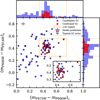 |
Fig. A.1 Same as Fig. 3 but extending the selection region in the (mF475W − mF606W)0 colour up to 0.75 for including the anomalous GC. |
Following the same methodology, we also use the (mu − mF475W)0 colour to further clean GC candidates. Fig. A.2 shows the colour-colour diagram with the three colours (similar to Fig. 4) and Fig. A.3 shows the distribution of the (mu − mF475W)0 colours (similar to Fig. 5). None of the additional GC candidates has a (mu − mF475W)0 colour compatible with our criterion. The anomalous spectroscopically confirmed object is too faint in the u-band for reliably getting its (mu − mF475W)0 colour. Therefore, at this point we have 36 GC candidates, only the spectroscopically confirmed object is added to the sample.
Following the same steps in this work, we statistically characterise the GC population, i.e. perturbing the measured parameters of the candidates based on the errors obtained from the completeness tests (see. Sect. 3.4 and Appendix B). The expected population of GCs results in 35 ± 3. After adding the completeness correction due to the limited depth of the data, we end up with 36 ± 3. To summarise, if we consider all the 20 spectroscopically confirmed GCs, we add one extra spectroscopically confirmed GC, and 3 extra objects in the expected population of GCs (from 32 ± 3 to 35 ± 3 GCs candidates).
Remarkably, the final number of objects does not significantly change even if the selection range in the colour (mF475W − mF606W)0 is twice as large as in the main analysis. As stated in Sect. 5.1 when comparing with the results from Marleau et al. (2024) and especially from Danieli et al. (2022), the colour range is really important for an adequate selection of GC candidates. However, the confirmed GC is located in a relatively clean region in colour space (Fig. A.1), making our results robust whether we include this object or not.
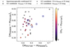 |
Fig. A.2 Same as Fig. 4 but applying a wider selection region to include the anomalous GC. Most of the new candidates have very red colours and are rejected due to their (mu − mF475W)0 values. |
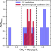 |
Fig. A.3 Same as Fig. 5 but applying a wider selection region in the (mF475W − mF606W)0 colour for including the anomalous GC. |
The measured properties of the confirmed anomalous object are listed in the last row of Table C.1. It is remarkable that, even though the profile and the fit of a Gaussian/King profile of this object look fairly normal, it shows large values of χ2red. Neither the imaging nor the results of the fits provide an obvious explanation to its anomaly.
Appendix B Photometric and morphological accuracy
To assess the completeness, photometric and morphological errors of our GC sample, we have performed tests in which we inject, retrieve and analyse artificial GC-like sources. These artificial GC-like sources have the colours of the spectroscopically confirmed GCs (i.e. (mF475W − mF606W)0 = 0.44, (mF606W − mF814W)0 = 0.41, and (mu − mF475W)0 = 1.20, see Sect. 3.3 for details). The mock GCs were subjected to the same analysis as the real data. For the HST data, we model the GCs by circularising the mean profile of the spectroscopically confirmed GCs (therefore having an ellipticity = 0 and FWHM = 2.7 px, see Sect. 3.1). For the u-band data, the model is based on a PSF constructed by circularising the radial profile of bright and non-saturated stars in the image (ellipticity = 0 and FWHM = 4.3 px, see Sect. 3.3). The profiles have been extended with the same power-law used for correcting the photometry in the analysis of real sources. We injected these artificial GCs (500 per magnitude bin) randomly distributed throughout the image with magnitudes between 21 and 28. Fig. B.1 show the results of these tests. The detection completeness represents the rate of recovered simulated GCs per magnitude bin (upper left panel). We have also compared the injected and recovered values of magnitude (lower left), ellipticity (upper right) and Re (lower right; given in pc assuming a distance of 20.7 Mpc).
In the HST data, the completeness limit (for objects simultaneously detected in the three filters) drops below 90% at mF606W ∼ 26.5 mag (blue dashed line in Fig. B.1). The errors at this magnitude are : ∼0.15 mag in photometry, 0.08 in ellipticity and 1.5 pc in Re. In the case of the u-band, the completeness drops below 90% at mu∼ 25.8 mag (corresponding to mF606W ∼ 24.3 mag, purple dashed line). The photometric error in the u-band at this magnitude is 0.3 mag.
Appendix C Properties of the GC candidates of MATLAS-2019
Table C.1 lists the properties of the confirmed and candidates GCs of MATLAS-2019. Magnitudes are corrected from Galactic extinction and aperture corrections as described in Sect. 3.2. Candidates with no given magnitude in the u-band are too faint to be measured in the u-band. The magnitude errors are obtained from the completeness tests (Appendix B) and combined with the uncertainty in the correction due to finite apertures.
The errors for the effective radius based on SExtractor are based on the mock GC tests (Appendix B) and the error for the values obtained from fitting Gaussian and King profiles are obtained from the typical difference between the Gaussian Re and the King Re.
Appendix D Ultra deep imaging of MATLAS-2019 with OSIRIS+: observational strategy and data reduction
Our ground-based, ultra-deep imaging of MATLAS-2019 was obtained using the instrument OSIRIS+ at the GTC. The field of view of OSIRIS+ is 7.8′ × 8.5′ (7.8′ × 7.8′ without vignetting). The OSIRIS+ setup represents a comprehensive upgrade of the OSIRIS instrument, implemented in 2022. This upgrade includes installing OSIRIS at the Cassegrain focal station and using a new blue-sensitive monolithic detector. The camera comprises one CCD detector with a pixel scale of 0.254 ″/pixel. In this configuration, we observed MATLAS-2019 with the u, g, and r filters on four separate nights, from the 18 to 26 April 2023. In Table 2, we report the total exposure time per filter, the surface brightness limits, and the FWHM of the PSF.
Appendix D.1 Dithering pattern
To achieve the depths required for a detailed study of MATLAS-2019 (µg ∼ 31.0 mag/arcsec2, 3σ in areas equivalent to 10″ × 10″), we need an accurate estimation of the illumination of the sky at the moment of the observations. Since the twilight flats provided by the observatory are not good enough for our goals (differences between twilight illumination and illumination of the observed field), we need to use the science exposures themselves for building the flat-field and correcting the illumination of the field at once. To account for this, we followed an observational strategy similar to that used in previous works with GTC and other large telescopes (LBT, Gemini; see Trujillo & Fliri 2016; Trujillo et al. 2021; Golini et al. 2024). The size of the dithering step has to be similar to the size of the galaxy, so we applied a dithering scheme with a 1′ shift and individual exposure times of 180 seconds. In this way, the galaxy is placed at different positions in the CCD, allowing a better determination of the sky background.
Appendix D.2 Data Reduction
The data were downloaded from the GTC Archive11 and reduced using a similar procedure as in Trujillo et al. (2021). Here, we describe the main steps of the process. All the pipeline steps rely on the Gnuastro Software (Akhlaghi 2018) and its tasks, as described below.
Appendix D.2.1 Bias and Flat field correction
First, for each image of each filter, we masked all detector defects of the CCD. We also mask all pixels with values greater than 6.5 × 10⁴ ADUs to account for saturation. After this, we corrected the images from bias. To do so, we created a masterbias by combining the individual bias frames with a sigma clipping median using the Gnuastro’s task Arithmetic. This masterbias is later subtracted from all science images.
For building the flat, we first normalise science images (bias-corrected) using the resistant mean of the values inside a ring that defines a constant-illumination section, centred on the centre of the CCD. Then, we combine the normalised, bias-subtracted science images to build a flat. However, instead of using all the images to build a master flat, we use the ones that are close in time for each image, thus allowing us to better characterise the sky illumination at the moment of the observation (Saremi et al. 2025). We define the number of frames to combine for building each of the flat-fields to be 10, characterising the field illumination on a 30 min. window. The strategy for building the flat-field is iterated a total of three times. The first flat-field is built by simply combining the images with a sigma-clipping median stacking, while on following iterations we also mask all the undetected signal before the combination. Each of this iterations improve the quality of the data, allowing us to improve the generated masks and further improve the flat itself. To avoid vignetting problems towards the corner of the detectors, we removed all the pixels where the flat-fields have a value lower than 90% the value of the central pixels.
Appendix D.2.2 Astrometry, photometry, and sky determination
We calculated an astrometric solution using Astrometry.net (v0.94; Lang et al. 2010). We used the Panoramic Survey Telescope and Rapid Response System (Pan-STARRS) DR1 (Chambers et al. 2016) as our astrometric reference catalogue. This produced a first astrometric solution, that we improved using SCAMP (v.2.10.0; Bertin 2006). SCAMP reads catalogues generated from SExtractor (v.2.25.2; Bertin & Arnouts 1996) and calculates the distortion coefficient of the images. After running SCAMP, we run SWarp (Bertin 2010) on each individual image to put them into a common grid of 3500 × 3500 pixels, using as resampling method LANCZOS3.
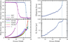 |
Fig. B.1 Results of the tests of the injection of mock GCs. Top left: Completeness of the HST data when simultaneously detecting the injected GCs in the three HST bands (blue line) and for the OSIRIS+ u-band (purple line). Bottom left: photometric errors for all the bands used in characterising the GCs of MATLAS-2019. Top right: ellipticity errors in the WFC3/F606W, where the ellipticity is measured. Bottom right: Re errors in the WFC3/F606W, converted to pc assuming a distance of 20.7 Mpc. The dashed vertical lines indicates when the detections fall below 90%. |
Once the astrometry is computed, we subtracted the sky of the individual frame by masking all sources using NoiseChisel. For each frame, we calculated the median value of the non-masked pixels and removed it from the original frame.
The calibration of the data (i.e. converting the pixel values from ADUs to physical units) is achieved by matching the fluxes of stars in our images to the fluxes of stars in an already-calibrated survey. The survey used for the calibration is The Dark Energy Camera Legacy Survey (DECaLS) DR10 (Dey et al. 2019) for the g and r, and the Sloan Digital Sky Survey (SDSS) DR17 (Abdurro’uf et al. 2022) for the u-band.
The calibration has been done as follows. First, the survey’s images (DECaLs and SDSS) in the different filters of MATLAS-2019’s field were downloaded, and catalogues of sources were generated. Later, in order to get a clean sample of bona fide stars, the catalogues are matched with Gaia DR3 stars. To minimise the noise introduced in the calibration we want to maximise the number of stars used, so instead of using just stars identified in Gaia, we look at the range of FWHM that these stars have, using it as a criterion for selecting point-like sources in the survey’s images. Then we perform the photometry of the selected sources by using large enough apertures, which ensures that we virtually measure all the flux of the point-like source. If the aperture were too small, some flux would be lost in the tails of the PSF, generating inconsistencies when comparing fluxes measured on different images due to the differences in the PSFs. The use of a large number of stars effectively washes out the effect of the contaminants introduced by the large aperture. For defining the aperture to use, a wide range of apertures have been explored, studying at which value the measured flux is stable, concluding that apertures of r = 9Re are optimal. Then the same process is applied to the data to calibrate, obtaining a catalogue of point-like sources to be used for the calibration. The apertures used for measuring the flux are r = 7Re. Additionally, to use non-saturated stars with high S/N, only sources with a magnitude between a certain range (16.0 < mag < 18.5, 19.5 < mag < 20.5, and 19.0 < mag < 20.0 for the u, g and r bands, respectively) have been used for the calibration. Applying these criteria, we end up having between 10 to 30 stars (depending on the filter) for calibrating each of the frames.
Since the photometric calibration is a complex task, surveys have non-negligible offsets between them. Thus, in order to be able to fairly compare data calibrated with different surveys, we decide to reference our calibration to an arbitrary but common framework, this being the Gaia spectra. This introduces a correction to be performed to the fluxes measured in DECaLS and SDSS, which are compared with the fluxes measured from the Gaia spectra and corrected (by applying an offset) to match them. Secondly, in order to give a precise photometry, we need to take into account the transmittance of the filters involved in the calibration. Even if technically we are working with the same filters (in this case u, g, r), there are differences in the filter response between the filters of different telescopes. This can be alleviated by applying a colour correction. The colour correction applied has been characterised based on the colour (g − r) and is determined using the survey’s filter shapes, the shapes of our filters, and GAIA spectra from stars in the field.
Finally, we match the catalogues and calculate the factor that we need to apply to our frames in order to have them calibrated to physical units. The factor computed for each frame is slightly different (due to noise and the available stars depending on the specific pointing), but since the frames to be combined in each reduction have been taken with the same configuration and parameters (same instrument, filter, exposure time, etc…) we apply the median value of the distribution of factors, reducing thus the noise in the calibration. The zero-point has been set to 22.5 in the AB magnitude system.
Properties of the GC candidates identified in MATLAS-2019.
Appendix D.2.3 Image co-addition and final stack
In the final step of the data reduction, individual exposures are combined to create a final mosaic image. This step is driven by the fact that observational conditions change throughout the night, as a number of factors like the air mass, (which varies depending on the position of the target in the sky) and meteorological events like passing clouds can affect the sky brightness, degrading its quality and generating artificially high standard deviations in the sky background pixel values, indicating poorer image quality. In light of this, images captured under better conditions should carry more weight in the final mosaic to enhance the accuracy of low surface brightness features. Thus, a weighted average is used to combine the images. The weight assigned to each image is determined by the quadratic ratio of the standard deviation of the sky in the best exposure to the standard deviation of the sky in the ith frame (i.e.  , where σmin corresponds to the standard deviation of the less noisy frame). However, before stacking the data in this manner, it is crucial to mask out pixels that have been affected by undesired signals like cosmic rays. For doing this, a sigma-clipping rejection per pixel is applied using all the exposures that are going to be combined.
The co-added image is significantly deeper than any individual image and, therefore, previously invisible low surface brightness features emerge from the noise. These features subtly affect the sky determination of our individual science images, and for this reason, it is necessary to mask these regions and repeat the entire sky determination process on the individual exposures with an improved mask. In short, we repeat the sky estimation (and subsequent reduction steps) described above on the individual images using the improved masks generated by this first data co-addition. The mosaics for our three photometric bands are derived using the same data reduction pipeline. The final stacks have a field of view of about 10′ × 12′, and are shown separately in Fig D.1. The colour image obtained from the final stacks is shown in D.2.
Appendix E Globular cluster system asymmetry
As pointed out in Sect. 5.2, the distribution of globular clusters of MATLAS-2019 shows an apparent asymmetry, with a larger number of candidates to the north-west. To test whether this excess of GC is statistically significant, we computed its significance using two different approaches.
First, we calculate the angular orientation of the axis that creates the maximum difference in the number of GCs between the two sides or hemispheres it separates. That results is an angle of ∼45◦12. We divide the GCs on both sides of this axis: 23 objects in one hemisphere and 12 in the other. We then derive the probability that the GCs are distributed in this way using a binomial distribution, due to the fact that the diffuse light of the galaxy is symmetric. The probability of having a distribution of GCs as the one in MATLAS-2019 is ∼2.4%.
Secondly, in addition to the difference in GCs between hemispheres, we consider the median distance from the galaxy centre to the GCs, as it also plays a role in the perceived over density of GCs. We produce 50 000 tests where we randomly distribute 35 GCs on the galaxy, assuming that the GC population follows the same distribution as that of the diffuse light, but reduced by a factor of Re,GC/Re = 0.7. In each realisation, we compute the axis that maximises the difference of GCs between hemispheres (as previously done). We also compute the distance of each GC to the centre of the galaxy. Fig. E.1 shows the results of the tests. We plot the difference between the number of sources in both hemispheres against the ratio of the median GC distance in each hemisphere. To compute this ratio, we assume that the side with a larger number of GCs (N1) goes in the numerator (R1), i.e. it is always larger than the unit. For the sake of clarity, we show the contours enclosing the 68%, 95% and 99.7% of realisations. The star marker indicates the observed value for the GCs of MATLAS-2019, falling at the boundary between the 95% and the 99.7% contour. In the light of this, we cannot exclude the possibility that the distribution of GCs in this galaxy is coincidental.
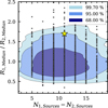 |
Fig. E.1 Probability of obtaining a GC distribution with certain parameters. The GC distribution is given by the difference in the number of GCs between two sides or hemispheres (x-axis) and the ratio between the median distance of the GCs (y-axis). The regions enclosing a 68%, 95% and 99.7% of the data are indicated in different hues of blue. The star located between de 95% and 99.7% regions correspond to the GC distribution of MATLAS-2019. |
Appendix F Distance to MATLAS-2019
Appendix F.1 Measurement of Re of the GCs of MATLAS-2019
Thanks to the high angular resolution of HST, the GCs of MATLAS-2019 are partially resolved. This allows us to extract morphological information from them such as the Re. We use pyimfit (a python wrapper for imfit, Erwin 2015) to fit of a function which approximates the intrinsic profile of a GC (a Gaussian and a King profile) convolved with the PSF of the images. We need a realistic PSF of the images, and since the PSF on space is fairly asymmetrical, the PSF derived from circularising of the 1D models obtained in Sect. 3.1.2 is not good enough for the measurements. Thus, to approximate the PSF in 2D, we simply use a bright, non-saturated and non-contaminated star located at RA: 15h05m18.66s and Dec: +1d47m46.61s. The image used for the fits is the WFC3/F606W image as it is the deepest.
We perform the fits in stamps of the sources of 81 px × 81 px. The background has been estimated in the same region as for the photometry (see Sect. 3.2), masking any neighbouring sources.
The first intrinsic profile assumed has been a Gaussian, where the only free parameter (σ) has been allowed to vary freely. The second model explored has been the King model (King 1962), which is described by a core and a tidal radius. The core radius is typically between less than one pc and a few pc, so at the proposed distances a conservative range is defined from 0.15 to 2 px. For the tidal radius, the range is between 20 and 100 pc, even though larger values are not unusual (See e.g. Peterson & King 1975; Harris et al. 2002; Barmby et al. 2007). Therefore, we only impose a lower value for the tidal radius of 2.5 px (around 10 pc). For the fits, the ellipticity was constrained between 0 and 0.2. To sum up, the ranges for the parameters of the fits are the following:
-
Gaussian prof.
0◦ ≤ PA ≤ 180◦
0 ≤ Ellipticity ≤ 0.2
σ ≥ 0
-
King prof.
0◦ ≤ PA ≤ 180◦
0 ≤ Ellipticity ≤ 0.2
0.15 px ≤ rc ≤ 2.0 px
rt ≥ 2.5 px
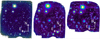 |
Fig. D.1 Entire mosaics 10′×12′ field around MATLAS-2019 obtained with OSIRIS+. From left to right u, g, and r band. |
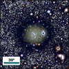 |
Fig. D.2 A region of 140″×140″around MATLAS-2019. The figure is a composite of an RGB image using the u, g and r OSIRIS+ bands and a black and white g + r background. North is up, and east is to the left. |
We provided pyimfit with an error map which is the standard deviation of the background region around each source.
Appendix F.2 GCLF and Re calibrations
The values explored in Sect. 5.3 for the peak of the GCLF are:
MV,TO = −7.66 ± 0.09 - MW - Metal poor GCs - (Di Criscienzo et al. 2006)
MV,TO = −7.40 ± 0.09 - MW - (Di Criscienzo et al. 2006)
MV,TO = −7.56 ± 0.02 - dIrr - (Georgiev et al. 2009b)
The conversion for MATLAS-2019’s globular clusters magnitudes between Vega and AB is V606(AB) = V(Vega) - 0.145 mag. This is derived computing V606(AB) and V(Vega) of a simple stellar population model from Vazdekis et al. (2016) with [Fe/H] = −1.44 and age 10 Gyr.
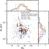 |
Fig. F.1 Comparison between the MV and Re of the GC population of MATLAS-2019 with the GCs from the Milky Way (Harris 1996), from nearby dwarf galaxies (Georgiev et al. 2009a) and from dwarf galaxies in the MATLAS survey (Poulain et al. 2025). The assumed distance to MATLAS-2019 is 20.7 Mpc. |
The values explored for the peak of the Re distribution are:
Log(Re,TO) = 0.520 ± 0.0236 pc - GCs from Dwarfs
Log(Re,TO) = 0.506 ± 0.0239 pc - GCs from MW
The estimates for the Re have been obtained directly from the catalogues (Harris 1996; Georgiev et al. 2009a), using a 3σ-clipped mean after transforming the radii to logarithmic scale. The errors given are the errors of the mean value of the distribution, (i.e. the standard errors).
Appendix F.3 Comparison with local GCs and MATLAS survey dwarfs GCs
We compared the distribution of magnitudes and Re of the GCs of MATLAS-2019, at the two possible distances of the galaxy, with the properties of local MW GCs (Harris 1996), GCs from nearby dwarfs (Georgiev et al. 2009a), and of GCs from dwarf galaxies from the MATLAS survey Poulain et al. (2025). These are shown in Figures F.1 at 20.7 Mpc and F.2 at 26.5 Mpc.
Looking at the local sample we see how magnitudes and effective radius seems not to show any trend, and how most of them occupy the region between −4.0 < Mv < −11 mag and 0.5 < Re < 10 pc. The comparison of MATLAS-2019 GC population with the locals allows us to visually inspect how alike are the populations depending on the distance.
All Tables
5σ limiting depths using apertures twice the FWHM of the GC profiles for each of the images used to identify the GC candidates of MATLAS-2019.
All Figures
|
Fig. 1 GC radial profiles in the WFC3/F606W band for the 20 spectroscopically confirmed GCs (grey). The blue line shows the S/N weighted mean profile of the GCs. We also plot the profile of the empirical PSF provided by the STScI in green, and the profile of the PSF obtained directly from stars of the images in orange. The vertical dashed red line (0.″6, equivalent to 15 px in WFC3 imaging) indicates where the profile is truncated, the vertical dotted brown line shows the FWHM of the mean GC profile, and the light blue region indicates where the background has been estimated. |
| In the text | |
|
Fig. 2 Normalised histograms of the effective radius (in parsecs, assuming a distance of 20.7 Mpc), ellipticity and F606W magnitude of different samples of sources; N is the number of sources in each bin and Nmax the maximum of their respective histograms. The grey histogram shows all the sources of the catalogues in grey (446 sources), the red hatched histogram the 20 spectroscopically confirmed GCs and the blue histogram the sources which fulfil the selection criteria (128 sources). The vertical dashed lines indicate the ranges of the GC selection, in each of the parameters. |
| In the text | |
|
Fig. 3 (mF475W − mF606W)0 vs (mF606W − mF814W)0 colour-colour diagram of the initial sample of GC candidates. The 20 spectroscopically confirmed GCs (Müller et al. 2020; Haacke et al. 2025) are shown as red squares. The orange dashed box indicates the region we have selected for our next sample of GC candidates and corresponds to ±3σ around the median colours of the confirmed GCs (excluding the anomalous object, see Sect. 3.3). The violet star, and its error bar, shows the prediction from Bruzual & Charlot (2003) models for an SSP of [Fe/H] = –1.44 dex and 9.1 Gyr (Müller et al. 2020). The inset shows a zoom-in into the dashed orange box for ease of viewing. The error bars shown in the upper-left corner are the errors of an object located at the peak of the GCLF (mF606W = 23.77 mag, assuming a distance of 20.7 Mpc to the galaxy). |
| In the text | |
|
Fig. 4 (mF475W −mF606W)0 vs (mF606W −mF814W)0 colour-colour diagram of GC candidates, colour-coded with the (mu − mF475W)0 colour. The 20 spectroscopically confirmed GCs (Müller et al. 2020; Haacke et al. 2025) are shown as squares and the candidates as circles. The size of the marker indicates the mF606W of the source, as shown in the legend. The sources in grey are objects that are too faint to be measured in the u-band. The blue open circles highlight those objects rejected based on their (mu − mF475W)0 colour. |
| In the text | |
|
Fig. 5 Normalised histograms of the (mu − mF475W)0 colour of the GCs of MATLAS2019; N is the number of sources in each bin and Nmax the maximum of their respective histograms. The red hatched histogram shows the spectroscopically confirmed GCs and the blue histogram the GC candidates. Only sources with trustable magnitude in the u−band are shown (i.e. mu < 25.8, see Sect. 3.3). The dashed vertical black lines indicate the ±3σ cut applied for GC selection. |
| In the text | |
|
Fig. 6 HST WFC3/F606W image convolved with a Gaussian kernel (σ = 1.5) showing the spatial distribution of the GC candidates identified in this work. The red circles indicate the GCs spectroscopically confirmed in Müller et al. (2020) and Haacke et al. (2025) while the blue circles highlight the GCs candidates and the orange circle represent the anomalous GC. The yellow dashed circles indicate 1Re, 2Re and 3Re of the galaxy (Re = 17.″2, Müller et al. 2020). |
| In the text | |
|
Fig. 7 Comparison of radial profiles in the WFC3/F606W band. We show the profiles of the spectroscopically confirmed GCs, the GC candidates obtained in this study in grey, the profile of the PSF from stars in green, and the profiles of 4 candidates located at more that 2Re from the galaxy’s centre in red. |
| In the text | |
|
Fig. 8 Surface brightness, ellipticity, and PA radial profiles of MATLAS-2019. The left panel shows the u-band (blue), g-band (teal) and r-band (red) surface brightness profiles as a function of the semi-major axis obtained with a fixed centre and ellipticity (ϵ = 0.07). The surface brightness profiles have been corrected from extinction. The right panel shows the position angle (top) and ellipticity (bottom) profiles from letting the parameters of the fit vary freely. |
| In the text | |
|
Fig. 9 Upper panel: OSIRIS+ colour (g − r)0 radial profile of MATLAS-2019. Bottom panel: the surface stellar mass density profile of MATLAS-2019. The density profile shows a break around ∼33″, coinciding with a change in the colour profile. |
| In the text | |
|
Fig. 10 Radial distribution of GC candidates in MATLAS-2019. The red profile represents the spectroscopically confirmed GCs, the GC candidates obtained in this study are in blue, and the whole GC system in green. The black line is the mass density profile of MATLAS-2019, as indicated in the right Y-axis. The errors in the GC profiles are the Poissonian error of the number of GCs per area in each annulus (i.e. |
| In the text | |
|
Fig. 11 Left panel: globular cluster luminosity function of MATLAS-2019. Middle panel: distribution of Re assuming that the intrinsic shape of the GC is a Gaussian. Right panel: distribution of Re assuming that the intrinsic shape of the GC is a King model. The spectroscopically confirmed GCs from Müller et al. (2020) and Haacke et al. (2025) are indicated in red (hatched), the population identified in this study is in blue. The widths of the bins have been calculated using the Freedman–Diaconis rule (Freedman & Diaconis 1981). The black solid line shows a Gaussian fit to the data. |
| In the text | |
|
Fig. 12 Distance to MATLAS-2019. The left panel shows the different estimates where the Re,GC is obtained assuming that the GC intrinsic profile follows a Gaussian model, while the right panel assumes a King model. Each of the points shows a different method or calibration used to estimate the distance to MATLAS-2019 as labelled. The grey box separates the distances obtained in Müller et al. (2021) and in Danieli et al. (2022). The (*) indicates the distance assumed in Danieli et al. (2022) based on the distance to the NGC5846 group. In the red box, we plot the weighted mean distance obtained using the different estimates for the GCLF and Re,GC methods. |
| In the text | |
|
Fig. A.1 Same as Fig. 3 but extending the selection region in the (mF475W − mF606W)0 colour up to 0.75 for including the anomalous GC. |
| In the text | |
|
Fig. A.2 Same as Fig. 4 but applying a wider selection region to include the anomalous GC. Most of the new candidates have very red colours and are rejected due to their (mu − mF475W)0 values. |
| In the text | |
|
Fig. A.3 Same as Fig. 5 but applying a wider selection region in the (mF475W − mF606W)0 colour for including the anomalous GC. |
| In the text | |
|
Fig. B.1 Results of the tests of the injection of mock GCs. Top left: Completeness of the HST data when simultaneously detecting the injected GCs in the three HST bands (blue line) and for the OSIRIS+ u-band (purple line). Bottom left: photometric errors for all the bands used in characterising the GCs of MATLAS-2019. Top right: ellipticity errors in the WFC3/F606W, where the ellipticity is measured. Bottom right: Re errors in the WFC3/F606W, converted to pc assuming a distance of 20.7 Mpc. The dashed vertical lines indicates when the detections fall below 90%. |
| In the text | |
|
Fig. E.1 Probability of obtaining a GC distribution with certain parameters. The GC distribution is given by the difference in the number of GCs between two sides or hemispheres (x-axis) and the ratio between the median distance of the GCs (y-axis). The regions enclosing a 68%, 95% and 99.7% of the data are indicated in different hues of blue. The star located between de 95% and 99.7% regions correspond to the GC distribution of MATLAS-2019. |
| In the text | |
|
Fig. D.1 Entire mosaics 10′×12′ field around MATLAS-2019 obtained with OSIRIS+. From left to right u, g, and r band. |
| In the text | |
|
Fig. D.2 A region of 140″×140″around MATLAS-2019. The figure is a composite of an RGB image using the u, g and r OSIRIS+ bands and a black and white g + r background. North is up, and east is to the left. |
| In the text | |
|
Fig. F.1 Comparison between the MV and Re of the GC population of MATLAS-2019 with the GCs from the Milky Way (Harris 1996), from nearby dwarf galaxies (Georgiev et al. 2009a) and from dwarf galaxies in the MATLAS survey (Poulain et al. 2025). The assumed distance to MATLAS-2019 is 20.7 Mpc. |
| In the text | |
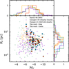 |
Fig. F.2 Same as Fig. F.1 but assuming a distance to MATLAS-2019 of 26.5 Mpc. |
| In the text | |
Current usage metrics show cumulative count of Article Views (full-text article views including HTML views, PDF and ePub downloads, according to the available data) and Abstracts Views on Vision4Press platform.
Data correspond to usage on the plateform after 2015. The current usage metrics is available 48-96 hours after online publication and is updated daily on week days.
Initial download of the metrics may take a while.