| Issue |
A&A
Volume 706, February 2026
|
|
|---|---|---|
| Article Number | A61 | |
| Number of page(s) | 14 | |
| Section | Astrophysical processes | |
| DOI | https://doi.org/10.1051/0004-6361/202557555 | |
| Published online | 30 January 2026 | |
PSR J0537–6910: Exponential recoveries detected for 12 glitches
1
Instituto Argentino de Radioastronomía (CCT La Plata, CONICET; CICPBA; UNLP), C.C.5, (1894) Villa Elisa Buenos Aires, Argentina
2
Facultad de Ciencias Astronómicas y Geofísicas, Universidad Nacional de La Plata Paseo del Bosque B1900FWA La Plata, Argentina
3
Departamento de Física, Universidad de Santiago de Chile (USACH) Av. Víctor Jara 3493 Estación Central, Chile
4
Center for Interdisciplinary Research in Astrophysics and Space Sciences (CIRAS), Universidad de Santiago de Chile Av. Víctor Jara 3493 Estación Central, Chile
5
Jodrell Bank Centre for Astrophysics, Department of Physics and Astronomy, The University of Manchester Manchester M13 9PL, UK
6
Department of Physics and Astronomy, Haverford College 370 Lancaster Avenue Haverford PA 19041, USA
7
SRON – Space Research Organisation Netherlands Niels Bohrweg 4 2333 CA Leiden, The Netherlands
8
Department of Space, Earth and Environment, Chalmers University of Technology SE-412 96 Gothenburg, Sweden
★ Corresponding author: This email address is being protected from spambots. You need JavaScript enabled to view it.
Received:
3
October
2025
Accepted:
8
December
2025
Abstract
Context. Pulsar rotational glitches are unresolved increments of the rotation rate that sometimes trigger an enhancement of the spin-down rate. On occasion, the augmented spin-down decays gradually over days or months in an exponential manner. This is observed particularly after the largest glitch events. Glitches and their exponential recoveries are attributed to the presence of a neutron superfluid inside pulsars. The young pulsar PSR J0537−6910 exhibits the highest known glitching rate, with 60 events detected over nearly 18 years of monitoring.
Aims. Despite most PSR J0537−6910 glitches being large, only one exponential recovery has been reported, following its first discovered glitch. This is puzzling as pulsars of similar age, rotational properties, and glitching behaviour typically present significant exponential recoveries. We wish to understand if this is an intrinsic difference of PSR J0537−6910 or a detectability issue due, for example, to its high glitch frequency.
Methods. The full dataset, including recent NICER observations, was systematically searched for evidence of exponential relaxations. Each glitch was first tested for evidence of recovery across a broad range of trial timescales. Good candidates were further investigated by identifying the best recovery models with and without an exponential term, then comparing them using Bayesian evidence.
Results. We discovered six new glitches, bringing the total number of glitches in this pulsar to 66. Our search and selection criteria strongly indicate the presence of 11 additional, previously undetected, exponential recoveries. We provide updated glitch and timing solutions. Exponential recoveries were detected only for the largest glitches (Δν > 20 μHz), though not for all of them. The inferred exponential timescales vary between 4 and 37 d, with the decaying frequency increment being close to or below 1% of the total in general. We find that the second derivative of the spin frequency (ν¨) can remain fairly stable across several glitches, and only some glitches are associated with persistent ν¨ changes. In particular, ν¨ tends to take its lowest values after glitches with exponential recoveries, corresponding to inter-glitch braking indices nig ∼ 6–9. On the other hand, following glitches without exponential recoveries – even large ones – ν¨ tends to be higher, with varied values that typically lead to braking indices above 9 (inferred nig mostly clustered between 10 and 35).
Key words: methods: observational / pulsars: general / pulsars: individual: PSR J0537-6910
© The Authors 2026
 Open Access article, published by EDP Sciences, under the terms of the Creative Commons Attribution License (https://creativecommons.org/licenses/by/4.0), which permits unrestricted use, distribution, and reproduction in any medium, provided the original work is properly cited.
This article is published in open access under the Subscribe to Open model. This email address is being protected from spambots. You need JavaScript enabled to view it. to support open access publication.
1. Introduction
Pulsars are rapidly rotating neutron stars that emit radiation across multiple wavelengths, from radio to gamma rays. They have extremely high and stable moments of inertia, which give them remarkably steady rotations. This places them among the most accurate clocks in the Universe (Hobbs et al. 2012).
However, the smooth rotation of pulsars can sometimes be interrupted by sudden increases in rotational frequency ν, called glitches (Espinoza et al. 2011; Manchester 2018; Zubieta et al. 2023). In addition, these spin-up episodes often exhibit a sudden change in the pulsar spin-down rate, which then recovers, sometimes partially in an exponential-like manner (Yu et al. 2013; Liu et al. 2024). Currently, around 700 glitches have been detected in more than 200 pulsars1, with a wide range of amplitudes: observed frequency changes Δν vary from ∼10−4 μHz to nearly 100 μHz (Basu et al. 2022).
Glitches are believed to be the manifestation of a sudden angular momentum transfer between a loosely coupled superfluid interior and the rest of the star (Baym et al. 1969; Anderson & Itoh 1975; Haskell & Melatos 2015; Antonopoulou et al. 2022; Zhou et al. 2022). The neutrons in the inner crust and core of neutron stars are in a superfluid state, which is characterised by irrotational flow with vanishing friction. Inside fast-rotating pulsars, however, it is energetically favourable for the superfluid to follow the rotation of its normal surroundings whilst remaining irrotational in its bulk. It does so by forming many microscopic vortices with non-superfluid cores, which carry all circulation and whose density determines a local, average rotation rate. As the pulsar spins down, vortices move outwards and eventually vanish at the superfluid boundary, so that the superfluid decelerates as well. If in some stellar layer this vortex motion is prevented by forces that ‘pin’ vortices to the normal matter, excess vorticity builds up because the pulsar spins down whilst the local superfluid maintains a higher rotation rate. Eventually, either due to the increasing velocity difference between the components or aided by some external disturbance, a catastrophic unpinning event takes place: vortices move, quickly transferring the excess angular momentum to the crust, which spins-up at a glitch.
Weakly coupled superfluid regions lag behind the abrupt glitch-induced increase in the crust’s rotation rate and temporarily decouple, reducing the effective moment of inertia upon which the external spin-down torque acts. This causes a transient increase in the spin-down rate  , commonly observed to accompany glitches, with typical amplitudes up to
  . In a considerable minority, mostly consisting of large glitches in young pulsars, part of this change exponentially decays over characteristic relaxation timescales of days to several weeks: a signature of superfluid components slowly recoupling to the crust (Haskell & Melatos 2015; Haskell et al. 2020; Antonopoulou et al. 2022). For well-monitored neutron stars with regular large glitches, such as the Vela pulsar, detected decaying timescales range from minutes (Dodson et al. 2002; Palfreyman et al. 2018; Ashton et al. 2019; Zubieta et al. 2025b) to ∼500 d (Zubieta et al. 2024). The study of glitches, and particularly their relaxation process, is key to understanding the internal physics of neutron stars.
PSR J0537−6910 stands out as the fastest spinning (ν ∼ 62 Hz), non-recycled, rotation-powered pulsar with the highest known spin-down energy loss rate (Ė ∼ 4.88 × 1038 erg s−1). It is a young object, associated with the 1–5 kyr old supernova remnant N157B in the Large Magellanic Cloud (Wang & Gotthelf 1998; Marshall et al. 1998), and it is by far the most frequently glitching pulsar with a rate of approximately three events per year and a total of 60 reported glitches in nearly 18 years of cumulated data (Middleditch et al. 2006; Antonopoulou et al. 2018; Ferdman et al. 2018; Ho et al. 2022). About 70% of these glitches are large, with Δν > 10 μHz (90% above 1 μHz), which contribute to the peak at large values observed in the bimodal distribution of glitch sizes for all glitching pulsars (Fuentes et al. 2017).
Glitches in PSR J0537−6910 are accompanied by significant increases in the spin-down rate  , which dominate
  -time evolution (Fig. C.1), a common feature of glitching pulsars of similar age, such as Vela (Lyne et al. 2015; Espinoza et al. 2017). On shorter timescales, these pulsars exhibit inter-glitch
  values that are considerably larger than the predictions of any model for pulsar braking. For example, the dipole braking model, in which the neutron star loses energy exclusively by magnetic dipole radiation, assuming constant moment of inertia and magnetic field, predicts a
  rate that is 20 times lower than the observed values between glitches in PSR J0537−6910. Contrary to similar (glitching) pulsars, however, PSR J0537−6910 does not feature prominent exponential relaxations, and their presence has been somewhat under-explored (Ho et al. 2020). The first glitch observed was the largest and the only one for which an exponential recovery was clearly discernible and well-studied (Antonopoulou et al. 2018).
In this work, we present six new glitches detected in recent NICER (Neutron star Interior Composition Explorer) observations of PSR J0537−6910 and analyse all known glitches in the entire dataset for the presence of exponential recoveries. In Sect. 2, we summarise the reduction process of the X-ray data from NICER and RXTE (Rossi X-ray Timing Explorer). In Sect. 3, we develop a systematic methodology to identify and characterise post-glitch exponential recoveries. In Sect. 4, we provide a report on the six new glitches and the results of our search for exponential recoveries on the 66 total glitches observed so far. Finally, in Sect. 5, we discuss the implications of our findings.
2. Observations
PSR J0537−6910 was discovered in the X-ray band in 1998 (Marshall et al. 1998), and only recently some weak and dispersed radio pulses were detected (Crawford et al. 2005; Crawford 2024). Monitoring its rotation with RXTE began on 1999 January 19 and lasted until 2011 December 31. Regular observations resumed 5.45 years later with NICER (Ho et al. 2020). In this work, we used all available RXTE and NICER data for this pulsar and calculated pulse times of arrival (TOAs) by cross-correlating pulse profiles with a pulse template. The RXTE TOAs used in our analysis are the same as those in Antonopoulou et al. (2018), derived using a method similar to that presented by Kuiper & Hermsen (2009) for PSR J1846−0258.
However, the template used for correlating with the folded profiles to obtain a TOA measurement comes from fitting a 60-bin asymmetric Lorentzian to a high signal-to-noise profile. In some cases, consecutive observations from RXTE were combined to achieve sufficient exposure for confidently measuring the spin frequency of the pulsar. This occurred mainly with observations performed after 2006, where generally only one or two of the five proportional counter units (PCUs) were operational during a standard observation.
For the NICER data, the methodology was laid out in Ho et al. (2020): HEASOFT 6.22–6.35.1 (Nasa High Energy Astrophysics Science Archive Research Center (Heasarc) 2014) and NICERDAS 2018-03-01_V003-2025- 03-11_V013A were used to process and filter the observations. We only kept events in the 1–7 keV range, where the pulse is easily detected (Kuiper & Hermsen 2015). As for RXTE data, there were some cases for which sets of close individual observations had to be merged to significantly detect the pulsar period. The typical total exposure of merged observations ranged between 4 and 9 ks. From each merged observation, one TOA was obtained. In this case, TOAs were measured by correlating the folded profiles with a template obtained from fitting a Gaussian to a series of NICER high signal-to-noise pulse profiles.
3. Methods
In the following, we discuss the 45 glitches published by Antonopoulou et al. (2018) for the complete RXTE observing period (MJD 51197–55926), plus 15 reported glitches from NICER observations, which we enumerate from 46 onward. Timing solutions for glitches 46–53 can be found in Ho et al. (2020) (glitches 1–7 in their work); glitches 54–56 were presented in Abbott et al. (2021) (glitches 8–10 in their work); and glitches 57–60 in Ho et al. (2022) (11–15 in their work).
We processed the latest NICER data (after MJD 59627) and report here on six new glitches that we identified and measured. Therefore, a total of 66 PSR J0537−6910 glitches were included in our post-glitch recovery analysis.
3.1. Pulsar timing
The pulsar rotation is monitored by recording TOAs of detected pulses and comparing them to the predictions of a spin-down model for the rotation phase ϕ, which can be approximated by a truncated Taylor series:
 (1)
(1)
where ν0,  and
and  are the rotation frequency of the pulsar and its first and second derivatives, respectively, at the reference epoch t0. The differences between the observed and predicted arrival times are called timing residuals. These can be remarkably small, thanks to the accuracy of TOA measurements and the stability of the pulsar’s rotation. Glitches introduce well-known signals in the residuals and, unless they are too small, are generally straightforward to identify.
To describe the changes in the rotation of the pulsar due to a glitch at time tg and its post-glitch recovery, an additional phase ϕg must be added to the model of Eq. (1) for t > tg, of the form (e.g. Yu et al. 2013; Zubieta et al. 2025a):
![Mathematical equation: $$ \begin{aligned} \phi _\mathrm{g} (t)&= \Delta \phi + \Delta \nu _\mathrm{p} (t-t_\mathrm{g} ) + \frac{1}{2} \Delta \dot{\nu }_\mathrm{p} (t-t_\mathrm{g} )^2 \nonumber \\&\quad +\frac{1}{6} \Delta \ddot{\nu }_\mathrm{p} (t-t_\mathrm{g} )^3 + \left[1-\exp {\left(-\frac{t-t_\mathrm{g} }{\tau _\mathrm{d} }\right)} \right]\Delta \nu _\mathrm{d} \, \tau _\mathrm{d} . \end{aligned} $$](/articles/aa/full_html/2026/02/aa57555-25/aa57555-25-eq14.gif) (2)
(2)
The quantities Δνp,  , and
, and  describe persisting changes in the rotational parameters with respect to the pre-glitch model, whilst a non-zero Δϕ might be required due to the uncertainty of the precise glitch epoch tg. The last term describes a transient component of the spin-up, Δνd, which exponentially relaxes on a timescale τd. Glitches can have one or more such exponential components in their recoveries; however, in this study of PSR J0537−6910 we examine glitch models with a maximum of one exponential term. We computed the total, unresolved initial frequency step as Δν = Δνp + Δνd and its recovery factor as Q = Δνd/Δν. The equivalent change in frequency derivative is
  , and it is useful to also define the spin-down rate recovery factor as
  (Weltevrede et al. 2011).
3.2. Post-glitch recovery searches
We analysed each glitch (n) using TOAs between the previous glitch (n − 1) and the following one (n + 1). Within this data span, we used TEMPO2 to fit Eq. (1) to the pre-glitch TOAs. If an exponential recovery was detected for glitch n − 1, we excluded any TOAs clearly affected by it from the pre-glitch data span used to characterise the following glitch n. This ensured that the pre-glitch-n data could be accurately described solely by Eq. (1). In general, PSR J0537−6910 has a high inter-glitch  , which can be determined even for short time intervals. We therefore included this term in the fits except in cases of exceptionally short (four or fewer TOAs) pre-glitch datasets, for which we set
  (Ho et al. 2020).
Indications of exponential signatures in the post-glitch recovery were searched for automatically in each inter-glitch dataset comprising of at least six TOAs. The first step of our methodology was to make an initial estimate of the glitch size by fitting a glitch model with only Δϕ, Δνp, and  (maintaining
  ). Glitch parameters from the literature were used as a starting solution, when available. In the next step, the full glitch model of Eq. (2) was fitted for, with Δνd and all other parameters allowed to vary except for τd, which was set at a trial value. For each post-glitch dataset, we performed such fits for a range of possible relaxation timescales: all integer values between one day and four times the total length of the post-glitch data span were used as trials for τd. Exponential recoveries on shorter timescales could not be accurately determined due to the timing resolution of the dataset. Similarly, the exponential signature was hard to discern if the relaxation timescale was considerably longer than the post-glitch fitted interval.
The variations in the χred2 metric for each glitch fit with respect to τd were analysed. When a minimum was present, the search was refined around it, as exemplified in Fig. 1.
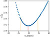 |
Fig. 1. Example of the exploratory process to determine possible values for an exponential relaxation timescale. The blue dots corresponds to the χred2 values of glitch 64, over a subset of the total range of trial τd values focused around the timescale that returns the minimum χred2 (marked by the red line). The dashed orange lines denote the 1σ uncertainty. These rather high χred2 values are used only to identify a possible timescale. Further analyses are performed for the final measurements (Table 2). |
This was not a final determination of glitch recovery but rather a preliminary exploration to identify whether the data favour a possible recovery timescale. Glitches for which the minimum χred2 occurred at either the beginning or the end of the explored τd range were not further explored. We assume in such cases that the absolute minimum might occur outside our trial τd range and therefore, as discussed above, we could not securely detect and characterise an exponential recovery with the available data.
For the final step, we considered two different glitch models to compare via marginal likelihood:
-
Model 1 (without recovery) consists of Δϕ, Δνp, and
 . We considered
  when its inclusion led to a significant decrease in the residuals’ RMS.
 -
Model 2 (with one exponential recovery) consists of Δϕ, Δνp,
 , Δνd, and τd. We incorporated
  when its inclusion led to a significant decrease in the residuals’ RMS. We used the best-fit recovery parameters from the previous step as initial values for these fits.
A nested sampling code2 (Skilling 2004) based on the PINT software (Luo et al. 2021) was used to fit the models and infer the most likely values for the glitch parameters. We explored a wide range for each parameter to ensure that a global solution was reached.
Finally, to decide the appropriate model for each glitch, we calculated their Bayesian evidences, Z1 and Z2, for Models 1 and 2, respectively, and assessed their logarithmic ratio:
 (3)
(3)
following the criterion used in Liu et al. (2024): if lnB21 < 2.5, Model 2 is considered to have insufficient evidence over Model 1. In the case of 2.5 < lnB21 < 5, Model 2 is considered to have moderate evidence over Model 1. For 5 < lnB21 < 10, strong evidence for Model 2 over Model 1 is considered. However, if lnB21 > 10, evidence for Model 2 is considered as decisive.
We treated all glitches for which the evidence for Model 2 was moderate, strong, or decisive as detections of exponential relaxations. In some cases, the posterior distributions for certain parameters are considerably asymmetric, and therefore we used the posterior mode – instead of the mean value – as the representative value for each parameter. From these, we constructed and used a timing solution for each glitch as a starting solution for a final fit, obtained using PINT. In most cases, the final fit only marginally reduced the RMS of the residuals compared to the starting solution. The difference between the modes and the values obtained after this fit was consistently smaller than the range defined by the 68% of the most likely values in the posterior distributions, even for the most asymmetric posteriors. We assigned final parameter uncertainties calculated as the distance from the mode to the 16th and 84th percentiles of its posterior samples.
4. Results
4.1. Detection of six new glitches with NICER
In the timing residuals of the most recent NICER data used in this analysis (MJD 59626–60601), the presence of six new glitches is evident – and in accordance with the known glitching rate of this pulsar. We present the parameters that describe these new glitches in Table 1.
Timing solutions (without exponential recovery terms) for the six new glitches detected with NICER.
To be consistent with earlier measuring techniques and to ensure the results are directly comparable to previously published glitch parameters, we followed Ho et al. (2020) and used TEMPO2 (Hobbs et al. 2006) to fit Eqs. (1) and (2) without the exponential relaxation term to the TOAs of each pre-glitch and post-glitch interval (described in Table A.1). A seventh new glitch (67) occurred around MJD 60592. Therefore, we include glitch 66 in the analysis but not glitch 67, since the post-glitch data were incomplete at the time of this analysis (see Ho et al. 2026).
Five out of the six new glitches have inferred amplitudes Δνp > 15 μHz, and all had detectable changes in  . As we discuss next, two of these glitches present evidence for exponential relaxation in their post-glitch recovery. Refined solutions that include this term are presented in the following subsection.
4.2. Detection of exponential post-glitch relaxations
We analysed a total of 66 PSR J0537−6910 glitches following the methods outlined in Sect. 3.2, starting from initial solutions presented in Antonopoulou et al. (2018), Ho et al. (2020), Abbott et al. (2021), Ho et al. (2022) and Table 1 of this work. We found 12 glitches for which the Bayesian criterion points to the presence of an exponential recovery, with moderate evidence in two cases and strong or decisive evidence in the other ten. These glitches are presented in Table A.2, together with information on the chosen solution for Models 1 and 2, as well as their Bayesian evidences.
Some glitches yielded a clear τd value during the initial systematic search, but their Bayesian evidence was not high enough to favour Model 2 over Model 1. This is likely due to the sparsity of post-glitch TOAs in these particular cases. Nonetheless, in these cases where Model 2 was favoured, the accuracy of the inferred exponential solutions does not appear strongly sensitive to variations in data quality. No clear correlation exists between the uncertainties of the inferred exponential parameters (Δνd and τd) and the TOA cadence or TOA errors of the respective post-glitch interval.
As noted in Table A.2, for some glitches Model 1 required a  in order to produce reasonably flat residuals; however, when the recovery term (Model 2) was added, the change
  became negligible. There were also two cases (glitches 43 and 45), for which including a
  term did not significantly flatten the residuals for Model 1; nonetheless, the exponential recovery term in Model 2 did. Finally, there were four cases for which both
  and a recovery term were required to significantly reduce the RMS of the residuals. In the model of the first glitch, we omitted
  , as we obtained only a few pre-glitch TOAs and therefore could not reliably determine
  before the glitch. Similarly,
  was not included for glitch 47, as only three pre-glitch TOAs were available. In this case,
  was fitted to both pre- and post-glitch data.
The final solutions of Model 2 for the 12 glitches with evidence of an exponential term in their post-glitch recovery are shown in Table 2. The description of the observations used for each fit is presented in Table A.3. It is worth mentioning that for glitches 12 and 47, a fraction of the posterior samples of Δνd is consistent with 0, as indicated by their respective uncertainties. Nevertheless, we consider them significant detections because the modes of the posteriors are far from zero, and the Bayesian criterium favours an exponential term. These two glitches have short inferred τd values, so the lack of TOAs immediately after the glitch hampers their accurate measurement, as reflected by their uncertainties. The shorter (∼3 d) recovery timescales seen in Table 2 emphasise the need to monitor PSR J0537−6910 with high resolution immediately after its glitches, to detect and resolve such fast transients. Such observations will also improve our detection capability for exponentials of any timescale.
Solutions for glitches exhibiting exponential recovery.
4.3. The exponential post-glitch relaxations
In Fig. 2, we show two of the clearest detections of exponential relaxations in PSR J0537−6910. For completeness, in Fig. B.1 we also show two large glitches for which we found no evidence of exponential signatures. Plots for all 12 glitches are available in a GitHub repository3.
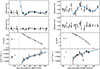 |
Fig. 2. Examples of exponential glitch recovery detections, for glitches 1 (left) and 56 (right). From top to bottom: Phase residuals relative to Model 1, with the residuals of the most likely exponential recovery model (Model 2 relative to Model 1) superimposed (blue curve); phase residuals relative to Model 2; frequency residuals relative to Eq. (1) fitted to TOAs up to the glitch epoch, with the post-glitch data all lowered by a certain amount (the mean post-glitch frequency residual) for better visualisation; and |

The exponentially relaxing component represents only a small fraction of the instantaneous change in spin frequency at the glitch. The inferred decaying amplitudes Δνd range between 0.05 and 0.8 μHz, while the persisting changes Δνp lie between 20 and 43 μHz. Therefore, the percentage of the initial frequency step that decayed exponentially, Q, is < 4% for all glitches. Most often, the calculated Q is close to or below 1%, which is typical of giant glitches in other pulsars (see, for instance, Zubieta et al. 2023).
It is remarkable that among the glitches with an exponential recovery, two (43 and 45) did not exhibit persistent changes  nor
nor  . For these glitches, the value of Q′ reaches 100%, meaning
  returned to its pre-glitch value once the exponential decay was completed. Similar high Q′ values are obtained for glitches 12 and 38. This is somewhat unusual for Vela-like glitches but has been observed in other pulsars, such as the Crab.
Although the persistent Δνp value does not change significantly with the addition of the exponential recovery term, the overall glitch and timing solution is altered. To investigate how including the exponentially recovering terms affects the inferred persisting  and
and  , we compare their values as calculated by Model 1 (no exponential) and Model 2 (one exponential term) in Fig. 3. As shown, the persistent spin-down change
  considerably decreases when exponential relaxation is included in the model. Particularly interesting are the cases of glitches 43 and 45, discussed above. For these, Model 1 required a Δ̇νp ≠ 0 term, which becomes zero for Model 2. This shows that, in some cases, exponential signatures may be misinterpreted as changes
  and
and  .
.
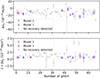 |
Fig. 3. Difference in inferred glitch parameters between Model 1 (blue points) and Model 2 (red points), for glitches with detected exponential recovery. Grey points represent values for glitches without detectable exponential terms (Model 1). |
The nominal timescales of the retrieved solutions for Model 2 span from 4 to 37 d, but are often highly uncertain (as seen in Table 2). To better capture the inferred range of typical recovery timescales of PSR J0537−6910, in Fig. 4 we show the distribution of τd values drawn from the posteriors of glitches with detected exponential recovery. There is some bimodality in the likely timescales, with a high peak around τd ∼ 3 d and a secondary one around τd ∼ 20 d. We note here that for those glitches where the inferred timescale was relatively long (glitches 1, 2, 43, 45, 64, and 65), we also tested a recovery model with two exponential terms but found no evidence for a second exponential. These results, which in general suggest short decaying timescales, intensify the need for dense observations as soon as possible after large glitches of PSR J0537−6910, in order to capture their short-term recovery behaviour.
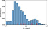 |
Fig. 4. Distribution of τd values for the 12 glitches with a detected recovery, as represented by a histogram of 10 000 samples (weighted) from the posterior distributions. The red ticks correspond to the values yielded by the final solutions, as reported in Table 2. |
Higher observing cadence close to a glitch will also allow us to place better limits on its size and improve the overall accuracy of all glitch parameters and timing solutions. Despite the small amplitude Δνd of the exponential relaxations compared to the total glitch change Δν, detecting and including these terms, when present, can affect several other results. This can be seen, for example, in Fig. 5, which displays the size Δν of a glitch versus the length of the time interval ΔTf until the following glitch. For PSR J0537−6910 these parameters are known to exhibit a strong, rather linear correlation (at least for intermediate to large glitches) (Middleditch et al. 2006; Antonopoulou et al. 2018; Ho et al. 2020, 2022). Here, we study the correlation between these two parameters through the Spearman rank-order correlation coefficient (SPEARMANR from the SCIPY library). We first consider all glitch amplitudes obtained via Model 1 (no exponential term) and find a correlation coefficient ρs = 0.89 with a p-value p = 1.5 × 10⁻²². Interestingly, when we instead use the sizes Δν retrieved by Model 2 for the 12 glitches with evidence of exponentials, the correlation measures improve to ρs = 0.94 and p-value of p = 2.0 × 10⁻³².
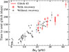 |
Fig. 5. Time to the next glitch as a function of Δνp for 66 glitches of PSR J0537−6910. Red markers indicate glitches for which an exponential recovery was detected. Using Model 2 solutions in these cases improves the size-waiting time correlation. Glitch 45, with a detected recovery, is the last glitch in the RXTE dataset, which ends 107 d after. Thus, the time to the next glitch is unknown, and it is plotted with a vertical arrow indicating the lower limit. The latest glitch reported in this work is glitch 66, which we are able to include in this plot as we know that glitch 67 occurred on MJD 60592. |
5. Discussion
Exponential recoveries were identified and measured following 12 glitches of PSR J0537−6910, all of which rank among the largest glitches observed. No evidence of exponential recovery was found for glitches with Δν < 20 μHz. For greater glitch sizes, some – but not all– events show an exponential component, and only the largest glitches (Δν ≳ 31.3 μHz) consistently exhibit detectable exponential terms. This behaviour can be seen in Fig. 5. By visually inspecting the timing residuals relative to a model – as in Eq. (2) – but without the exponential term, we confirm that no additional glitches of sizes between 20 and 30 μHz show obvious signs of exponential recovery. Nevertheless, not all residuals are adequately flat. For instance, the timing residuals for glitches 66 and 28, which are the first and second largest events without a detected recovery (with Δν = 31.3 μHz and Δν = 30.3 μHz, respectively), are sufficiently flat, similar to what is observed for glitch 9 (the fourth largest glitch without a recovery, with Δν = 26.4 μHz). However, glitch 51 (26.9 μHz), which is the third largest glitch without an exponential detection, exhibits noisier residuals relative to the same model. Other glitches within this size range behave similarly to these largest events, two of which are shown in Fig. B.1. We could not find any obvious reason – such as observational biases or failure to retrieve equally accurate solutions – for why exponentials were not detected after these large glitches. Furthermore, the presence of a detectable exponential relaxation seems associated with lower inter-glitch  values, as discussed below. It is thus possible that the differences in post-glitch behaviour are intrinsic to the pulsar. Future observations can reveal whether that is the case and what it depends upon.
5.1. Inter-glitch spin-down rate evolution
When the favoured glitch model includes an exponential term, the post-glitch rotation typically evolves with a lower  . This is not surprising at first, as all detections concern large glitches. These are followed by long (at least 100 d) inter-glitch intervals due to the aforementioned Δν-ΔTf correlation, and it has been shown that the inter-glitch
  tends to decrease over time from the glitch epoch (Andersson et al. 2018). To test this with our updated glitch sample, we fitted Eq. (1) to 90-day TOA intervals, starting after each glitch and moving forward by 20 days until the next glitch was reached. The resulting
  values as a function of time since the preceding glitch are shown in Fig. 6. With all glitches collectively considered,
  indeed appears to decrease over time. However, beyond ∼70 d the glitches without a detectable exponential have higher
  (blue points) compared to glitches with exponential relaxation (red circles). We emphasise that the modelled exponential contributions were been removed before calculating these
  values. If that had been the case, the red markers in Fig. 6 (circles and stars) would have been even lower, especially at early times. Therefore, we do not expect the blue points to be higher at late times due to unidentified exponentials of similar timescales as the detected recoveries. Although we cannot exclude contributions from undetected exponential relaxations on much longer timescales, given the current analysis and the broad range of trial timescales, this explanation seems considerably less likely than a different recovering regime.
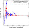 |
Fig. 6.
|


This genuine difference between glitches with and without detected exponential terms can also be expressed via the braking index. Assuming a power law  for the spin-down evolution, the braking index n can be calculated from observations as
  . Typical inter-glitch braking indices nig in Vela-like pulsars are nig = 10–40, or higher. This is arguably the result of internal superfluid torques (Espinoza et al. 2017; Antonopoulou et al. 2018) rather than external magnetospheric torques, which are expected to give much lower values (e.g. n ∼ 3 in the standard magnetic dipole braking model). Whilst for most glitches of PSR J0537−6910, the inter-glitch nig is generally greater than 9 and as high as 35; after the glitches with detected exponential recoveries, it settles to lower values, between 6.2 and 9.4.
To further investigate the  values between glitches and the overall rotational evolution, we studied
  as a function of time. A
  dataset was constructed by fitting Eq. (1) to overlapping subsets of data containing at least five TOAs and spanning at least 30 d, but not through glitches. For these fits we kept
  fixed at the mean value of each inter-glitch interval. The fitting window moved one TOA each time; hence, the data are heavily smoothed for visualisation purposes. In Appendix C we present the resulting
  evolution, resembling a sawtooth curve typical of pulsars with repeating large glitches (e.g. Espinoza et al. 2017). In the case of PSR J0537−6910,
  decreases over the years, with a corresponding effective negative slope and long-term negative effective braking index, a potential product of the high glitch activity (Antonopoulou et al. 2018; Ho et al. 2020). Between glitches,
  increases rapidly: the inter-glitch evolution has high, positive
  values and nig > 3, which likely involves contributions from (at least) the exponentially and non-exponentially recovering superfluid, as well as the external electromagnetic and magnetospheric torques.
The overall stability of the inter-glitch  can be observed in Fig. 7, where the modelled exponential and persisting glitch components are ‘corrected’ for, by subtracting
 ![Mathematical equation: $ [\Delta\dot\nu_{\mathrm{p}} - \exp(-(t-t_{\mathrm{g}})/\tau_{\mathrm{d}})\Delta\nu_{\mathrm{d}}/\tau_{\mathrm{d}}] $](/articles/aa/full_html/2026/02/aa57555-25/aa57555-25-eq159.gif) from
from  after each glitch. This results in the disappearance of the sawtooth curve and the long-term negative slope of
  observed in Fig. C.1, leaving a predominantly linear, smooth evolution under a remarkably stable positive slope (
 ). This high inter-glitch
  and some additional wandering features (above random scatter) seen in Fig. 7 remain unaccounted for by the current glitch model, which has only one exponential term to describe internal torques and does not for example include the response of non-linearly coupled superfluid components (Haskell et al. 2020). We performed separate linear fits for the RXTE and NICER data and found
  for RXTE and
  for NICER. The corresponding braking indices are high (nig = 16.49 ± 0.05 and nig = 18.4 ± 0.2, respectively) as in other similar glitching pulsars.
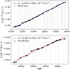 |
Fig. 7. Evolution of |

To better understand the variations in  , we subtracted (additionally to the corrections for the glitch components) a linear model with a fixed, reference value of
  Hz s−2, which corresponds to one of the lowest inter-glitch measurements of
  (observed after the first and largest glitch; nig = 6.8). These new residuals are shown in Fig. 8. As expected, the
  residuals are flat in the first inter-glitch interval; however, they also remain relatively flat after the second glitch (large, followed by an exponential relaxation), indicating that
  remains close to
  . However, around the time of the third glitch, which is large but has no detected exponential,
  increases and remains high until the next exponentially recovering glitch occurs (glitch 6), after which it decreases again and remains slightly above
  throughout several glitches. Similar patterns can be seen in the rest of the data:
  falls close to
  following glitches with detected exponentials but overall spends long periods around a higher, rather constant, value. This is clearest in the first half of the middle panel, when many glitches occurred but none had detectable exponentials:
  remains high and relatively constant for about 2000 days. Remarkably, some of the sharper increases in
  in Fig. 8 appear to occur around small glitches instead of intermediate or large ones (and never after an exponentially recovering glitch). To explore this possible relation between the inter-glitch
  and the size of the previous glitch, we plot the value of
  after each glitch, i.e.
  , against Δνp of the preceding glitch. The result is shown in Fig. 9, which shows a weak anti-correlation between
  and Δνp with the Spearman-rank correlation coefficient ρs = −0.314 and a p-value of p = 0.012.
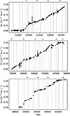 |
Fig. 8. Residuals of |

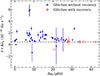 |
Fig. 9.
|


5.2.  and spin-down evolution
As the frequent, large persisting changes of the spin-down rate  are the most probable cause of the observed negative long-term trend of the spin-down evolution (Fig. C.1), we explored their correlations with the change of
  during the time intervals preceding and following the glitch. The results can be seen in Fig. 10. We calculated the change in the spin-down rate during the inter-glitch intervals as
  for the pre-glitch data span and
  for the post-glitch data span. Here, t− refers to the time since the previous glitch, and t+ refers to the time to the next glitch. Following Liu et al. (2024), the smallest glitches (Δν/ν < 10−7) were excluded from the analysis, and the waiting times were recalculated between the remaining glitches. We find a significant correlation between the increase in
  during an inter-glitch interval and its change
  at the subsequent glitch, with ρs = 0.79 and p-value = 9.3 ⋅ 10−13. This is in accordance with previous results for this particular pulsar (Middleditch et al. 2006; Antonopoulou et al. 2018). On the other hand, a correlation of
  with the change of
  in the time until the next glitch is not as tight, with ρs = 0.29 and p-value = 0.03, although such a correlation has been observed for several other pulsars (Lower et al. 2021; Liu et al. 2024). It was already noted in Liu et al. (2024) that both correlations are seen for some glitching pulsars, and that for PSR J0537−6910
  is more strongly correlated with the preceding (rather than following) increase in
  . Our results, which use the persisting changes (instead of the total change, which includes the exponentially relaxing components) further strengthen this conclusion. Because
  is a proxy of the amount of superfluid that recoupled since the previous glitch and is therefore available to decouple again at the next glitch causing a bigger
  , this correlation implies a ‘reservoir’ effect for the glitch
  changes in PSR J0537−6910 (Antonopoulou et al. 2018; Liu et al. 2024).
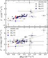 |
Fig. 10. Comparison between |


5.3. Distributions of Δνp,  , and waiting times
The number of glitches studied in this work (66) might be small by statistical standards, but it is the largest glitch sample from a single pulsar ever investigated. We therefore explored the distributions of basic glitch parameters (Δνp,  , and inter-glitch waiting times) using our updated measurements. The unbinned data were modelled using the STATS package of the SCIPY library. For visualisation purposes, we binned the data using the minimum histogram bin width between the Sturges rule and the Freedman-Diaconis estimator. Histograms of the glitch parameters are shown in Fig. 11, together with the fitted models for Gaussian distributions, which are an acceptable fit to the data.
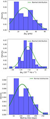 |
Fig. 11. Distribution of Δνp (top panel), |


We find that Δνp and  are consistent with normal distributions centred at 16 μHz and −11.3 × 10⁻¹⁴ Hz s−1, respectively, with p − value of 0.48 and 0.54. With respect to the inter-glitch waiting times, the p-value of the normal distribution is 0.22, and it is centred at μ = 108 days – in accordance to that in Fig. 5, which shows that a waiting time of ≈108 d corresponds to a Δνp ≈ 16 μHz. The parameters of the fitted distributions are presented in Table 3.
Description of the normal distributions of Δν,  , and the waiting times.
6. Conclusion
PSR J0537−6910 is the most frequently glitching pulsar, exhibiting an average of three glitches per year. Analysis of some recent NICER observations delivered the detection of six new glitches with properties typical for this pulsar (Table 1). With these new detections, the total number of published glitches for this pulsar is now 66. The vast majority of the glitches in PSR J0537−6910 are large compared to the majority of glitches detected in other pulsars, with 70% of them having Δν > 10 μHz. In other young pulsars, large glitches such as these are often followed by exponential-like recoveries. However, in the case of PSR J0537−6910, only one exponential recovery had been reported despite the detection of more than 50 large glitches. We performed a systematic search for exponential recoveries following all major glitches of PSR J0537−6910 and defined detection criteria based on model comparison and Bayesian evidence. Using this method, 11 new exponential recoveries were identified and characterised.
The presence of detectable exponential recoveries seems to depend on glitch size. Every glitch with sizes Δν above 31.3 μHz exhibits an exponential recovery, but only some glitches of amplitudes 20 μHz < Δν < 31.3 μHz do, and no exponentials are detected for any glitch with sizes below 20 μs. PSR J0537−6910 has a uniquely strong correlation between glitch size and the length of its following inter-glitch interval. This could introduce an observational bias as, for example, glitches with sizes below 10 μs are followed by only a ∼50 d interval, which might be too short to securely detect the exponential recovery. It cannot, however, account for the lack of detections for glitches with Δν ≳ 20 μs, which we believe may be an intrinsic behaviour of the pulsar.
For the detected recoveries, the measured Δνd values are between 0.05 μHz and 0.8 μHz, while τd ranges between 3 d and 37 d, which evidences the need for a high-cadence monitoring of this pulsar to thoroughly characterise its glitches. All the values of Q are below 4%, while Q′ consistently lie between 46% and 100%. Including exponential recovery in the timing model affects the inferred parameters, especially Δνp and  . We re-evaluated known correlations of this pulsar using the new solutions and find a very strong correlation between Δνp and the time until the following glitch, as well as a strong correlation between the change of
  over a pre-glitch interval t−, calculated as
  , and
, and  at the following glitch. We also find a mild anti-correlation between Δνp and its post-glitch value of
  . Importantly, it was demonstrated that the spin-down rate
  evolves at a lower
  following glitches with exponential recovery (once the exponential relaxation is over) compared to the generally stable evolution with higher
  following glitches without detected exponential decay.
Our models do not include a red noise component. While timing noise can certainly influence some of the inferred recovery parameters or even mimic an exponential relaxation, the combination of theoretical expectations, consistent trends across glitches, and the distinct residual structures strengthens our confidence that the majority of the detected exponential components represent real post-glitch behaviour.
These findings can help us understand the mechanism behind glitches and the superfluid recoupling process that follows them, as well as shed light on the interplay of various internal and externals torques for this pulsar. Continuous high-cadence observations of glitching pulsars are essential for studying neutron star dynamics, and PSR J0537−6910 is an excellent target for such monitoring due to its frequent, large glitches and unique characteristics. As we showed in this work, aspects of its rotational behaviour remain under-explored, and fast post-glitch transients require good time coverage to achieve further progress.
Acknowledgments
We thank Zaven Arzoumanian and Keith Gendreau for scheduling extra observations with NICER, which allowed the detection of some of the post-glitch recoveries reported here. CME acknowledges support from ANID/FONDECYT, grant 1211964. DA acknowledges support from an EPSRC/STFC fellowship (EP/T017325/1). WCGH acknowledges support through grant 80NSSC22K1305 from NASA. FG is a CONICET researcher. FG acknowledges support from PIBAA 1275 and PIP 0113 (CONICET). We used computing resources made available by ANID Chile SIA, grant SA77210112 (PI: Pinto). This work is supported by NASA through the NICER mission and the Astrophysics Explorers Program and uses data and software provided by the High Energy Astrophysics Science Archive Research Center (HEASARC), which is a service of the Astrophysics Science Division at NASA/GSFC.
References
- Abbott, R., Abbott, T. D., Abraham, S., et al. 2021, ApJ, 913, L27 [NASA ADS] [CrossRef] [Google Scholar]
- Anderson, P. W., & Itoh, N. 1975, Nature, 256, 25 [NASA ADS] [CrossRef] [Google Scholar]
- Andersson, N., Antonopoulou, D., Espinoza, C. M., Haskell, B., & Ho, W. C. G. 2018, ApJ, 864, 137 [Google Scholar]
- Antonopoulou, D., Espinoza, C. M., Kuiper, L., & Andersson, N. 2018, MNRAS, 473, 1644 [NASA ADS] [CrossRef] [Google Scholar]
- Antonopoulou, D., Haskell, B., & Espinoza, C. M. 2022, Rep. Prog. Phys., 85, 126901 [NASA ADS] [CrossRef] [Google Scholar]
- Ashton, G., Lasky, P. D., Graber, V., & Palfreyman, J. 2019, Nat. Astron., 3, 1143 [Google Scholar]
- Basu, A., Shaw, B., Antonopoulou, D., et al. 2022, MNRAS, 510, 4049 [NASA ADS] [CrossRef] [Google Scholar]
- Baym, G., Pethick, C., & Pines, D. 1969, Nature, 224, 673 [NASA ADS] [CrossRef] [Google Scholar]
- Crawford, F. 2024, American Astronomical Society Meeting Abstracts, 243, 132.04 [Google Scholar]
- Crawford, F., McLaughlin, M., Johnston, S., Romani, R., & Sorrelgreen, E. 2005, Adv. Space Res., 35, 1181 [Google Scholar]
- Dodson, R. G., McCulloch, P. M., & Lewis, D. R. 2002, ApJ, 564, L85 [Google Scholar]
- Espinoza, C. M., Lyne, A. G., Stappers, B. W., & Kramer, M. 2011, MNRAS, 414, 1679 [NASA ADS] [CrossRef] [Google Scholar]
- Espinoza, C. M., Lyne, A. G., & Stappers, B. W. 2017, MNRAS, 466, 147 [NASA ADS] [CrossRef] [Google Scholar]
- Ferdman, R. D., Archibald, R. F., Gourgouliatos, K. N., & Kaspi, V. M. 2018, ApJ, 852, 123 [Google Scholar]
- Fuentes, J. R., Espinoza, C. M., Reisenegger, A., et al. 2017, A&A, 608, A131 [NASA ADS] [CrossRef] [EDP Sciences] [Google Scholar]
- Haskell, B., & Melatos, A. 2015, Int. J. Mod. Phys. D, 24, 1530008 [NASA ADS] [CrossRef] [Google Scholar]
- Haskell, B., Antonopoulou, D., & Barenghi, C. 2020, MNRAS, 499, 161 [Google Scholar]
- Ho, W. C. G., Espinoza, C. M., Arzoumanian, Z., et al. 2020, MNRAS, 498, 4605 [Google Scholar]
- Ho, W. C. G., Kuiper, L., Espinoza, C. M., et al. 2022, ApJ, 939, 7 [Google Scholar]
- Ho, W. C. G., Kuiper, L., Espinoza, C. M., et al. 2026, MNRAS, accepted [Google Scholar]
- Hobbs, G. B., Edwards, R. T., & Manchester, R. N. 2006, MNRAS, 369, 655 [Google Scholar]
- Hobbs, G., Coles, W., Manchester, R. N., et al. 2012, MNRAS, 427, 2780 [NASA ADS] [CrossRef] [Google Scholar]
- Kuiper, L., & Hermsen, W. 2009, A&A, 501, 1031 [NASA ADS] [CrossRef] [EDP Sciences] [Google Scholar]
- Kuiper, L., & Hermsen, W. 2015, MNRAS, 449, 3827 [NASA ADS] [CrossRef] [Google Scholar]
- Liu, Y., Keith, M. J., Antonopoulou, D., et al. 2024, MNRAS, 532, 859 [Google Scholar]
- Lower, M. E., Johnston, S., Dunn, L., et al. 2021, MNRAS, 508, 3251 [NASA ADS] [CrossRef] [Google Scholar]
- Luo, J., Ransom, S., Demorest, P., et al. 2021, ApJ, 911, 45 [NASA ADS] [CrossRef] [Google Scholar]
- Lyne, A. G., Jordan, C. A., Graham-Smith, F., et al. 2015, MNRAS, 446, 857 [NASA ADS] [CrossRef] [Google Scholar]
- Manchester, R. N. 2018, in Pulsar Astrophysics the Next Fifty Years, eds. P. Weltevrede, B. B. P. Perera, L. L. Preston, & S. Sanidas, 337, 197 [NASA ADS] [Google Scholar]
- Marshall, F. E., Gotthelf, E. V., Zhang, W., Middleditch, J., & Wang, Q. D. 1998, ApJ, 499, L179 [Google Scholar]
- Middleditch, J., Marshall, F. E., Wang, Q. D., Gotthelf, E. V., & Zhang, W. 2006, ApJ, 652, 1531 [Google Scholar]
- Nasa High Energy Astrophysics Science Archive Research Center (Heasarc) 2014, Astrophysics Source Code Library [record ascl:1408.004] [Google Scholar]
- Palfreyman, J., Dickey, J. M., Hotan, A., Ellingsen, S., & van Straten, W. 2018, Nature, 556, 219 [NASA ADS] [CrossRef] [Google Scholar]
- Skilling, J. 2004, in Bayesian Inference and Maximum Entropy Methods in Science and Engineering: 24th International Workshop on Bayesian Inference and Maximum Entropy Methods in Science and Engineering, eds. R. Fischer, R. Preuss, & U. V. Toussaint (AIP), AIP Conf. Ser., 735, 395 [NASA ADS] [CrossRef] [Google Scholar]
- Wang, Q. D., & Gotthelf, E. V. 1998, ApJ, 494, 623 [Google Scholar]
- Weltevrede, P., Johnston, S., & Espinoza, C. M. 2011, MNRAS, 411, 1917 [NASA ADS] [CrossRef] [Google Scholar]
- Yu, M., Manchester, R. N., Hobbs, G., et al. 2013, MNRAS, 429, 688 [NASA ADS] [CrossRef] [Google Scholar]
- Zhou, S., Gügercinoğlu, E., Yuan, J., Ge, M., & Yu, C. 2022, Universe, 8, 641 [NASA ADS] [CrossRef] [Google Scholar]
- Zubieta, E., Missel, R., Sosa Fiscella, V., et al. 2023, MNRAS, 521, 4504 [Google Scholar]
- Zubieta, E., García, F., del Palacio, S., et al. 2024, A&A, 689, A191 [NASA ADS] [CrossRef] [EDP Sciences] [Google Scholar]
- Zubieta, E., García, F., del Palacio, S., et al. 2025a, A&A, 694, A124 [NASA ADS] [CrossRef] [EDP Sciences] [Google Scholar]
- Zubieta, E., Missel, R., Araujo Furlan, S. B., et al. 2025b, A&A, 698, A72 [NASA ADS] [CrossRef] [EDP Sciences] [Google Scholar]
Appendix A: Data intervals used to measure new glitches and exponential recoveries
Table A.1 gives details on the fits of six new glitches (Table 2). Table A.2 shows the Bayesian evidence of Models 1 and 2 for each glitch where model 2 was favoured. Table A.3 presents details of the fits of glitch exponential recoveries to 12 glitches (Table 2).
Data used to model six new glitches (Table 1).
Bayesian evidence for the models corresponding to the 12 positive detections.
Description of the data used to measure exponential glitch recoveries (Table 2).
Appendix B: Examples of glitches without a detected recovery
We present two examples of large glitches for which we did not detect exponential recovery. In these cases, the algorithm described in Sect. 3.2 either did not identify a minimum of χred2 within 1 day to 4 times the length of the data span, or, if it did, the Bayesian evidence for Model 2 was not significant compared to Model 1.
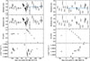 |
Fig. B.1. Examples of glitches 28 (left) and 51 (right) without a detected exponential recovery. From top to bottom: Phase residuals relative to Model 1, with the residuals (blue curve) of the most likely exponential recovery model (Model 2 relative to Model 1), corresponding here to zero, superimposed; phase residuals relative to Model 2; frequency residuals relative to Eq. 1 fitted to TOAs up to the glitch epoch, with the post-glitch data all lowered by a certain amount (the mean post-glitch frequency residual) for better visualisation; and |

Appendix C: Evolution of 
We present the evolution of  in Fig. C.1. The evolution shows a global negative slope, which is caused by repeated large glitches. The slope becomes positive when the effects of the glitches are removed.
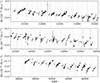 |
Fig. C.1. Evolution of the spin-down rate. For visual purposes, the quantity |
All Tables
Timing solutions (without exponential recovery terms) for the six new glitches detected with NICER.
Description of the data used to measure exponential glitch recoveries (Table 2).
All Figures
|
Fig. 1. Example of the exploratory process to determine possible values for an exponential relaxation timescale. The blue dots corresponds to the χred2 values of glitch 64, over a subset of the total range of trial τd values focused around the timescale that returns the minimum χred2 (marked by the red line). The dashed orange lines denote the 1σ uncertainty. These rather high χred2 values are used only to identify a possible timescale. Further analyses are performed for the final measurements (Table 2). |
| In the text | |
|
Fig. 2. Examples of exponential glitch recovery detections, for glitches 1 (left) and 56 (right). From top to bottom: Phase residuals relative to Model 1, with the residuals of the most likely exponential recovery model (Model 2 relative to Model 1) superimposed (blue curve); phase residuals relative to Model 2; frequency residuals relative to Eq. (1) fitted to TOAs up to the glitch epoch, with the post-glitch data all lowered by a certain amount (the mean post-glitch frequency residual) for better visualisation; and |
| In the text | |
|
Fig. 3. Difference in inferred glitch parameters between Model 1 (blue points) and Model 2 (red points), for glitches with detected exponential recovery. Grey points represent values for glitches without detectable exponential terms (Model 1). |
| In the text | |
|
Fig. 4. Distribution of τd values for the 12 glitches with a detected recovery, as represented by a histogram of 10 000 samples (weighted) from the posterior distributions. The red ticks correspond to the values yielded by the final solutions, as reported in Table 2. |
| In the text | |
|
Fig. 5. Time to the next glitch as a function of Δνp for 66 glitches of PSR J0537−6910. Red markers indicate glitches for which an exponential recovery was detected. Using Model 2 solutions in these cases improves the size-waiting time correlation. Glitch 45, with a detected recovery, is the last glitch in the RXTE dataset, which ends 107 d after. Thus, the time to the next glitch is unknown, and it is plotted with a vertical arrow indicating the lower limit. The latest glitch reported in this work is glitch 66, which we are able to include in this plot as we know that glitch 67 occurred on MJD 60592. |
| In the text | |
|
Fig. 6.
|
| In the text | |
|
Fig. 7. Evolution of |
| In the text | |
|
Fig. 8. Residuals of |
| In the text | |
|
Fig. 9.
|
| In the text | |
|
Fig. 10. Comparison between |
| In the text | |
|
Fig. 11. Distribution of Δνp (top panel), |
| In the text | |
|
Fig. B.1. Examples of glitches 28 (left) and 51 (right) without a detected exponential recovery. From top to bottom: Phase residuals relative to Model 1, with the residuals (blue curve) of the most likely exponential recovery model (Model 2 relative to Model 1), corresponding here to zero, superimposed; phase residuals relative to Model 2; frequency residuals relative to Eq. 1 fitted to TOAs up to the glitch epoch, with the post-glitch data all lowered by a certain amount (the mean post-glitch frequency residual) for better visualisation; and |
| In the text | |
|
Fig. C.1. Evolution of the spin-down rate. For visual purposes, the quantity |
| In the text | |
Current usage metrics show cumulative count of Article Views (full-text article views including HTML views, PDF and ePub downloads, according to the available data) and Abstracts Views on Vision4Press platform.
Data correspond to usage on the plateform after 2015. The current usage metrics is available 48-96 hours after online publication and is updated daily on week days.
Initial download of the metrics may take a while.