| Issue |
A&A
Volume 707, March 2026
|
|
|---|---|---|
| Article Number | A365 | |
| Number of page(s) | 15 | |
| Section | Astrophysical processes | |
| DOI | https://doi.org/10.1051/0004-6361/202555804 | |
| Published online | 20 March 2026 | |
Flux variability of the “10 keV feature” of 4U 0115+63
1
Dr. Karl-Remeis-Observatory and Erlangen Centre for Astroparticle Physics, Friedrich-Alexander-Universität Erlangen-Nürnberg, Sternwartstr. 7, 96049 Bamberg, Germany
2
University of Maryland, Department of Astronomy, College Park, MD 20742, USA
3
NASA Goddard Space Flight Center, Astrophysics Science Division, Greenbelt, MD 20771, USA
4
CRESST and Center for Space Sciences and Technology, University of Maryland, Baltimore County, 1000 Hilltop Circle, Baltimore, MD 21250, USA
5
Department of Astronomy, University of Geneva, Chemin d’Écogia, 16, 1290 Versoix, Switzerland
6
INAF, Osservatorio Astronomico di Brera, Via E. Bianchi 46, 23807 Merate, Italy
7
Department of Astronomy and Astrophysics, University of California San Diego, La Jolla, CA 92093, USA
8
European Space Agency (ESA), European Space Astronomy Centre (ESAC), Camino Bajo del Castillo s/n, 28692, Villanueva de la Cañada, Madrid, Spain
9
Howard University, Department of Physics and Astronomy, Washington, D.C., 20059, USA
10
NASA Goddard Space Flight Center, Astrophysics Science Division, Code 661, Greenbelt, MD 20771, USA
11
Embry Riddle Aeronautical University, 3700 Willow Creek Road, Prescott, AZ 86301, USA
12
Physics Dept., United States Naval Academy, Annapolis, MD 21402, USA
13
Dept. of Physics and Astronomy, George Mason University, Fairfax, VA 22030, USA
★ Corresponding author: This email address is being protected from spambots. You need JavaScript enabled to view it.
Received:
4
June
2025
Accepted:
4
February
2026
Abstract
Context. X-ray spectra of accretion-powered X-ray pulsars can often be described using a power-law continuum with a high-energy cutoff, which might be further modified by additional spectral components. The Be X-ray binary system 4U 0115+63 is well known for having one of the highest numbers of detected harmonics of its cyclotron resonant scattering features (CRSFs), a pronounced spectral component known as the “10 keV feature”, and quasiperiodic oscillations (QPOs) with a period of about 500 s during outbursts.
Aims. The changes in count rate by a factor of two during the ∼500 s QPOs allow us to probe the variation in the spectral components with flux. We study the “10 keV feature” in emission, aiming to disentangle it from the broadband continuum and CRSFs and investigate its origin.
Methods. We focus on the flux-dependent behavior of the CRSF and its harmonics, and particularly the contribution of the “10 keV feature”, as seen in the flux-resolved analysis of two NuSTAR observations of the 2015 outburst.
Results. Comparing the flux-resolved spectra of a given observation with the respective total dataset revealed a distinct change in overall spectral shape at the position of the “10 keV feature” but no comparable deviation at the energies of the harmonic CRSFs. The change associated with the “10 keV feature” does not seem to involve its centroid energy, which remains constant within a given observation. We find indications for an anticorrelation between the continuum flux and the ratio of the “10 keV feature” flux to the continuum flux within each observation.
Conclusions. The analysis strengthens previous claims that the “10 keV feature” shows some independence from the remaining features. This result supports the interpretation that the “10 keV feature” has a different formation mechanism than the continuum emission, although its origin lies within the same physical environment.
Key words: binaries: general / stars: emission-line / Be / pulsars: individual: 4U 0115+63 / X-rays: binaries
Deceased 17 June 2025.
© The Authors 2026
 Open Access article, published by EDP Sciences, under the terms of the Creative Commons Attribution License (https://creativecommons.org/licenses/by/4.0), which permits unrestricted use, distribution, and reproduction in any medium, provided the original work is properly cited.
This article is published in open access under the Subscribe to Open model. This email address is being protected from spambots. You need JavaScript enabled to view it. to support open access publication.
1. Introduction
Be X-ray binaries (BeXRBs) are a subclass of high mass X-ray binaries (HMXBs), where a neutron star (NS) is in an eccentric orbit around a Be-type star. They exhibit luminous X-ray outbursts when matter from the Be star’s decretion disk flows onto the NS. Two types of outbursts have been identified. Type I outbursts are periodic and typically occur when the accretor approaches periastron and accretes part of the decretion disk (Okazaki et al. 2013). Type II outbursts are more luminous, can last up to several weeks, show no dependence on orbital phase, and are probably caused by a strong misalignment between the decretion disk and the binary orbit (Martin et al. 2014; Martin & Charles 2024, and references therein). In the course of an outburst, the mass accretion rate onto the strongly magnetized NS can vary by several orders of magnitude, making BeXRBs especially useful laboratories to study accretion physics of NSs.
One particularly interesting system is 4U 0115+63, which undergoes giant type II outbursts that typically last one to two months every few years (Müller et al. 2013, and references therein, hereafter M13). Discovered as an X-ray source by Uhuru (Giacconi et al. 1972), 4U 0115+63 consists of a NS with the Be-type companion star V635 Cas (Unger et al. 1998; Negueruela & Okazaki 2001) in an eccentric (e = 0.34) orbit with a 24.3 d orbital period (Rappaport et al. 1978). The system is located at a distance of  kpc (Bailer-Jones et al. 2021)1. The NS has a spin period of ∼3.6 s (Cominsky et al. 1978). 4U 0115+63 is well known for its uniquely high number of cyclotron resonant scattering features (CRSFs). These features are created in the strong magnetic field at the poles of a NS and represent the energy difference between the discrete Landau levels. Transitions between nonadjacent levels lead to higher harmonic lines. For 4U 0115+63 a total of five harmonic lines were detected in the X-ray band (Santangelo et al. 1999; Heindl et al. 2000; Ferrigno et al. 2009). The fundamental line is at ∼12 keV, which is low compared to most other cyclotron line sources (Staubert et al. 2019) and corresponds to a magnetic field strength of ∼1012 G – similarly one of the lowest known among HMXB pulsars. Due to the high number of lines, modeling the continuum and lines requires very careful analysis. As discussed in detail by M13 and Bissinger né Kühnel et al. (2020, hereafter B20), when using a continuum description that yields physically meaningful parameters for the CRSF parameters, their energy is independent of the source luminosity. Based on an alternative model, other publications claim a very strong correlation between the luminosity and the CRSF energy (see e.g., Nakajima et al. 2006; Li et al. 2012; Roy et al. 2024); see Sect. 4 for further details and a discussion of the continuum models. Another prominent feature, visible in 4U 0115+63’s light curve, is its quasiperiodic oscillations (QPOs), with an amplitude of ∼2 in count rate on ∼500…900 s timescales found during its 1999 outbursts (Heindl et al. 2000) and also detected in later outbursts (Roy et al. 2019).
Of special interest to this work is 4U 0115+63’s spectral complexity. Generally, the X-ray spectra of HMXBs in outburst can be well described by power-law continua with a high-energy cutoff. However, additional components at intermediate energies are often required to adequately model the spectra. A complex structure of residuals around 10 keV is particularly common when using standard phenomenological models (Coburn et al. 2002; Manikantan et al. 2023). They can be effectively modeled by an additional broad Gaussian component, with a centroid energy of ∼10 keV, either in emission (for example, Vybornov et al. 2017; Thalhammer et al. 2021, for Cep X-4 and Cen X-3) or in absorption (see, for example, Fürst et al. 2014; Diez et al. 2022, for analysis of Vela X-1), commonly referred to as the “10 keV feature”.
4U 0115+63 is a system with a particularly complex intermediate energy region due to the presence of the fundamental CRSF, along with the onset of the spectral turnover. The “10 keV feature” at around ∼8 keV in emission in the spectrum of this source has been reported and discussed by, for example, Ferrigno et al. (2009), M13, and B20. It remains unclear whether this feature can be considered an independent physical component or if its presence merely reflects a more complex formation of the broadband continuum that cannot entirely be accounted for with a cutoff power law. Since the luminosity dependence of the other spectral features is well established, we address this issue by studying the behavior of the “10 keV feature” at different luminosities using the count rate variations in the QPOs. Up to now no proper explanation of the origin of these QPOs is given in the literature. For example, Roy et al. (2019) and Li et al. (2025) show that models commonly used for explaining QPOs in LMXBs can be ruled out, such as the beat or the Keplerian frequency model, disk precession, and thermal instabilities in the disk. The modulation also cannot be explained by variations in foreground absorption. While work on the origin of the QPO is clearly needed, a possible explanation consists of variations in the mass accretion rate at the poles, even though the physical origin of the modulation is unknown. For this purpose we analyze two observations, each performed with the Nuclear Spectroscopic Telescope Array (NuSTAR, Harrison et al. 2013) and the Neil Gehrels Swift Observatory (Swift, Troja 2020; Gehrels & Swift Team 2004), taken during the 2015 outburst of 4U 0115+63.
The paper is structured as follows. In Sect. 2, we introduce the NuSTAR and Swift observations of 4U 0115+63 and discuss the data reduction. Section 3 presents our timing analysis, while in Sect. 4 we present the averaged spectral analysis of the Swift and NuSTAR data. Section 5 covers the flux-resolved spectroscopy of the NuSTAR observations. We summarize and discuss our results on the “10 keV feature” and its origin in Sect. 6.
2. Outburst profile, data acquisition, and reduction
We analyze observations taken with NuSTAR and Swift during the bright type II outburst of 4U 0115+63 in 2015. This outburst started around 2015 October 15, lasted for about 30 days, and had a peak flux of ∼450 mCrab in the 15–50 keV band of Swift BAT (Fig. 1). See Table 1 for a log of observations. Data from the 2023 outburst yield similar results to those presented here and will be discussed in a separate publication.
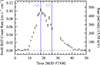 |
Fig. 1. Swift Burst Alert Telescope (BAT; Barthelmy et al. 2005) light curve of the 2015 outburst of 4U 0115+63 in the 15–50 keV band with a binning of 1 d. The blue-shaded regions highlight the quasi-simultaneous NuSTAR and Swift observation times. |
List of observations of 4U 0115+63.
4U 0115+63 was observed twice by NuSTAR during this outburst: first on 2015 October 22 for ∼9 ks (ObsID 90102016002; hereafter referred to as N1) during the outburst maximum at a 1–60 keV luminosity of ∼6.8×1037 erg s−1, and on 2015 October 30 for ∼15 ks (ObsID: 90102016004; hereafter called N2) at a luminosity of ∼4.4 × 1037 erg s−1. Here and in the following, luminosities were determined using a distance of 5.8 kpc (Bailer-Jones et al. 2021). The observation times are highlighted in Fig. 1. These two datasets have previously been analyzed by Roy et al. (2019), Liu et al. (2020), Manikantan et al. (2024) and Stierhof et al. (2025), with a different focus compared to this paper. We ignore NuSTAR data taken above 60 keV, which are strongly background-dominated. Data products were extracted using HEASOFT (version 6.30.1) and the NuSTAR calibration database (CALDB) (version 20220912) and reprocessed following The NuSTAR Data Analysis Software Guide2. Using newer software versions did not affect the following results. We chose circular extraction regions of 100″ radius centered on the source for the source region and placed background regions in the outer areas of the field of view.
To obtain a sanity check for our modeling of the soft X-ray absorption, we also utilized Swift X-ray telescope (XRT; Burrows et al. 2005) snapshot observations taken in window timing (WT) mode simultaneously with the NuSTAR observations N1 and N2, with exposure times of ∼2.4 ks (ObsID: 00081774001; hereafter S1) and ∼2.0 ks (ObsID: 00081774002; hereafter S2), respectively. Data products were extracted using HEASOFT (version 6.30.1) and Swift CALDB (version 20220803). We defined the source region with 22″ × 40″ rectangular boxes and the background region with a 25″ × 45″ area in a corner of the XRT chip. Previous discussions of these two observations are given by Tsygankov et al. (2016), Wijnands & Degenaar (2016), and Rouco Escorial et al. (2017). Since our aim is solely to check our treatment of the soft absorption, we performed a simultaneous fit to the 1.0–4.5 keV XRT-data and the 4.5–60 keV NuSTAR spectrum. These consecutive energy ranges avoid discrepancies due to known problems with cross-calibrating the two instruments (Madsen et al. 2020, 2021), as suggested by the NuSTAR Guest observer facility (K. Pottschmidt, priv. comm.). Further extending the energy ranges to enable overlap between the datasets leads to comparable results but increases systematic uncertainties due to detector calibration issues. For N1/S1 the best-fit NH-values agree with the NuSTAR-only fits, while for N2/S2 the combined fit yields a slightly higher value of NH at a level that does not affect our subsequent results. For this reason, and given that the XRT observations only cover a small part of the NuSTAR exposure time, we use Swift data only in our study of the average spectrum (Sect. 4), not in the flux-resolved analysis (Sect. 5).
3. NuSTAR light curves and the “500 s QPO”
Figure 2 shows the light curves of N1 and N2. The Swift snapshot times are highlighted by the green-shaded regions. As previously reported by, for example, Heindl et al. (1999), Dugair et al. (2013), and Ding et al. (2021), the source showed a strong ∼2 mHz QPO during N1 and N2, with maximum count rates of up to twice the average clearly visible on ∼500 s timescales. Figure 3 displays a representative section of the N1 light curve and the entire S1 light curve, which spans less than four full QPO cycles.
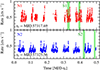 |
Fig. 2. N1 (top) and N2 (bottom) light curves, using combined data from FPMA and FPMB for clarity binned at three times the spin period of 4U 0115+63. The green-shaded regions highlight the observation periods of the S1 and S2 Swift snapshots. |
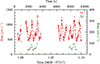 |
Fig. 3. Selected part of the 4U 0115+63 light curve, showing NuSTAR (red) and Swift (dark green) data highlighting the system’s strong QPOs. |
Using power spectral densities (PSDs) from N1 and N2 observations, which combine FPMA and FPMB, we can compare the variability seen here with the earlier RXTE-PCA observations from 1999 (Heindl et al. 1999). To cover a wide range of frequencies, we utilized light curves with initial binning ranging from 0.01 s to 100 s across the full NuSTAR energy range. We used the normalization by Miyamoto et al. (1991). The PSDs are shown in Fig. 4 superposed on the RXTE results from Heindl et al. (1999, their Fig. 5, black). The vertical solid orange lines indicate the NS spin frequency at ∼0.28 Hz and its higher harmonics. Their relative strengths are a measure of the complexity of the pulse profile. See, for example, the PSD of Vela X-1 discussed by Fürst et al. (2010). Two additional smaller peaks appear at 1.6 and 2.6 times the NS’s spin frequency, which are only visible in the NuSTAR data (Fig. 4, dashed lines). The discrepancy seen above ∼0.4 Hz is due to well-known dead-time effects in the NuSTAR data (Bachetti et al. 2015; Bachetti & Huppenkothen 2018).
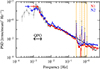 |
Fig. 4. PSDs of the NuSTAR observations, shown in red for N1 and blue for N2. For comparison the black data points indicate the results obtained by Heindl et al. (1999). The vertical solid orange lines highlight the spin frequency of the NS and its higher harmonics. The vertical dashed lines mark two additional peaks at 1.6 and 2.6 times the NS spin frequency. |
Since our work focuses on low-frequencies variability, we chose not to perform dead-time corrections to mitigate discrepancies at the high-frequency end of our dataset. At lower frequencies, the PSDs measured with NuSTAR and RXTE-PCA are very similar in amplitude and shape. In summary, 4U 0115+63’s variability remained remarkably constant between the two outbursts in 1999 and 2015. A timing analysis including the PSDs of the NuSTAR data from 4U 0115+63’s 2023 outburst was also performed by Jain et al. (2025). Their results are consistent with ours (except for their proper treatment of the Poisson noise correction at high frequencies, which we do not apply here). Li et al. (2025) performed a pulse-phase resolved analysis of 4U 0115+63’s millihertz QPOs in the 2023 observations. They found no luminosity dependence of the frequency but report that the power of the ∼1 mHz QPO is energy-dependent, while the 2 mHz power is not.
To study short term spectral changes during the QPO, we subdivided each NuSTAR observation into four different subsets. To generate the good time intervals (GTIs) corresponding to a given count rate range in the full NuSTAR energy range, we used 1 s binned light curves of the total observation. The selection criteria were chosen as follows. The light curve was first sliced every n × 100 counts s−1, where n is an integer. To facilitate spectral fitting with similar signal-to-noise ratios between the spectra, we combined these slices. The lowest count rate band required the greatest share of data with about 50% of the total counts, as it spans the longest observation time and thus includes the highest fraction of the background counts. For both observations this resulted in more than 106 counts per flux-resolved spectrum. The remaining data were then distributed approximately equally in the three higher bands. Each of the remaining count rate bands in the end held more than 2 × 10⁵ counts. Initial light curve slice size affected sorting flexibility but ensured better result reproducibility and reduced the personal selection bias. We named the flux-resolved spectra Ri.j, where i = 1, 2 corresponds to the N1 and N2 NuSTAR observations, respectively, and j = 1, 2, 3, 4 denotes the serial number from the lowest to highest rate band. The final selection of the rate bands for N1 and N2 is illustrated in Fig. 5. During the analysis, several other intensity selections were tested, focusing, for example, on QPO phase rather than purely on count rate (for details, see Berger 2022). We found that different intensity selections did not significantly change the results of the following analysis.
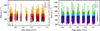 |
Fig. 5. Selected rates for extracting different flux-resolved spectra from N1 (left) and N2 (right) using 1 s binning. The selection criteria were chosen to be < 700 cts/s, 700–800 cts/s, 800–900 cts/s, and > 900 cts/s for N1 and < 500 cts/s, 500–600 cts/s, 600–700 cts/s, and > 700 cts/s for N2. |
4. Average spectrum and the “10 keV feature”
We now turn to the analysis of the spectra. We start with establishing the baseline spectral shape by analyzing the flux-averaged data and use it for the flux-resolved analysis in Sect. 5. We modeled the joint NuSTAR (4.5–60 keV) and Swift-XRT (1–4.5 keV) spectra using the Interactive Spectral Interpretation System (ISIS), version 1.6.2-51 (Houck & Denicola 2000). Both datasets were rebinned sufficiently to warrant the applications of χ2 statistics. Unless stated otherwise, all listed uncertainties are given at a 90% confidence level.
Due to the presence of the CRSFs, 4U 0115+63’s X-ray spectrum is notoriously difficult to model. M13 and B20 give an extensive discussion of the various empirical continuum models used in the literature. They show that a high number of different combinations of continua and CRSF models (some with and without a “10 keV feature”) yield formally correct descriptions of the data in a statistical sense. The choice between modeling approaches must therefore be based on physical assumptions, not solely on fit statistics. M13 and B20 show that continuum models based on the negative and positive exponential function or combinations of blackbodies with a power law yield cyclotron line parameters that are not physical. For example, B20 show in their discussion of the Iyer et al. (2015) model that the model component intended to describe the fundamental CRSF causes a relative continuum flux reduction of almost 90% (see Fig. 5 and Table 2 from B20). This reduction is inconsistent with our understanding of cyclotron scattering in accretion columns (e.g., Schwarm et al. 2017). Other line parameters found with these continua, such as their very large widths, also disagree with typical CRSF parameters from other sources and expected from accretion column theory. For instance, Li et al. (2012) modeled observations of the 2008 outburst with a fundamental cyclotron line as high in energy as ∼17 keV, and with higher harmonics starting at ∼23 keV. Notable in this approach is its very large width of almost 6 keV for the fundamental line and the decreasing widths for the higher harmonics. This behavior disagrees with what is expected from Doppler broadening, where σCRSF ∝ ECRSF (Meszaros & Nagel 1985b, their Eq. (1)). Applying this continuum model results in a CRSF energy-luminosity correlation widely cited in the literature (e.g., Li et al. 2012; Roy et al. 2024). However, M13 and B20 argue that this correlation appears as an artifact: the line components model changes in continuum slope and exponential cutoff with luminosity, rather than intrinsic CRSF behavior.
In this paper, we therefore concentrate on the implications of utilizing a simple empirical continuum model that, when applied to 4U 0115+63, yields CRSF parameters that are more in line with those seen in many CRSF sources (M13; B20), namely a power law with a high energy exponential cutoff,
 (1)
(1)
where Γ is the photon index and Efold the folding energy. We account for absorption in the interstellar medium using the absorption model by Wilms et al. (2000) with cross sections by Verner et al. (1996). Following B20, we describe emission from the ionized plasma in the vicinity of the X-ray source by including three additive narrow (σ = 10−6 eV) Gaussian emission lines describing the Fe Kα line at 6.4 keV, the Fe XXV Kα line at 6.69 keV, and the Fe XXVI Kα line at 6.97 keV. The centroids of the lines were taken from Kortright & Thompson (2000) and from the AtomDB Atomic Database. Above 7 keV, the X-ray continuum is heavily modified by cyclotron lines. We describe the lines as multiplicative absorption lines with Gaussian optical depth profiles modeled with the gabs function (Arnaud et al. 2022), parameterized by their strength DCRSF, width σCRSF, and energy ECRSF. Individual lines are differentiated by consecutive numbers, starting from 0 for the fundamental line. As we show below, the NuSTAR data have a sufficiently high signal-to-noise ratio (S/N) to detect four CRSFs. To avoid degeneracies of the line parameters with the continuum components, we fixed the energies of the harmonic lines to be integer multiples of ECRSF, 0. This approach is justified by earlier analyses (e.g., Pottschmidt et al. 2005, M13, and B20). We confirmed these results in a test spectral fit where we set ECRSF, n = cEnECRSF, 0 and found cE to never exceed ±5%. We therefore omitted this constant, as our analysis does not focus on CRSF energies.
Following the argument of Meszaros & Nagel (1985b, their Eq. (1)), we coupled the CRSF widths σCRSF, n to the respective line energy, using the constant cCRSF, σ. This approach mitigates nonphysical correlations between the CRSFs and the continuum introduced when the parameters are left free (M13; B20). Finally, we also included a multiplicative constant to account for uncertainties in the relative flux calibration of the instruments, normalizing all fluxes to that measured with NuSTAR-FPMA.
Other analyses, for example M13, used the cyclabs function instead of gabs to model the CRSFs. A detailed explanation of both functions is given in Arnaud et al. (2022). Fits to 4U 0115+63 with both CRSF models were compared and discussed by B20, who showed that both models can describe the spectra of 4U 0115+63 equally well. Therefore, the only benefit of choosing a specific model is comparability with previous results using the same model.
Consistent with earlier work, our analysis shows that a broad “10 keV feature” is required (for example, Ferrigno et al. 2009; Liu et al. 2020, M13; B20). Following M13, we added a Gaussian line profile to account for the presence of the “10 keV feature”, with width σ10 keV, energy E10 keV, and flux F10 keV. In another approach Farinelli et al. (2016) modeled the “10 keV feature” using cyclotron emission convolved with a varying magnetic field in the accretion column. B20 discuss the possibility of using a blackbody component to model the “10 keV feature” in 4U 0115+63 instead of a broad Gaussian, concluding that it does not provide a sufficient description of the component and leads to strong residuals below 10 keV. We can confirm this conclusion with our own unsuccessful attempts.
Finally, we modeled the spectra using a power law with a high energy exponential cutoff, four CRSFs, a broad Gaussian to account for the “10 keV feature”, and three narrow Gaussian features for the iron lines. The resulting best-fit parameters for the two sets of combined data from NuSTAR and Swift are listed in Table B.1; see Fig. 6 for the spectra and the respective best fit. The model describes the underlying spectra well, showing no systematic deviations in the residuals, resulting in a fit with χ2/d.o.f. = 660.6/441 = 1.50 for O1 and χ2/d.o.f. = 623.9/439 = 1.42 for O2. The reduced χ2 can in principle be further improved when relaxing the constraints on the CRSF parameters, for example by not coupling the line energies. However, as the additional constraints were required for the subsequent flux-dependent analysis, we maintained them to ensure comparability.
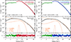 |
Fig. 6. Top: NuSTAR and Swift spectra of O1 (left) and O2 (right) with the best-fit model (black). The data from XRT are shown in green, FPMA in the lighter color, and FPMB in the darker color. Middle: Visualization of different model components. The data are shown in gray, and the model using the best-fit parameters is shown in black. The component contribution is shown in orange, using a dash-dotted line for the cutoff power law, a dashed line for the “10 keV feature”, and a dotted line for the iron lines. Bottom: Residuals of the best-fit model. |
5. Flux-dependence of the “10 keV feature”
In this section, we use 4U 0115+63’s QPOs to study the behavior of its spectral components, primarily the “10 keV feature”, at different flux levels on short time scales. To this end, we divided each observation based on the NuSTAR count rate (see Sect. 3) and conducted a spectral analysis on the flux-selected spectra. We maintained the assumptions from Sect. 4 for modeling the observation-averaged spectra, to ensure consistent fit approaches and perform the analysis solely based on the NuSTAR data due to lack of Swift coverage.
5.1. Flux-resolved spectroscopy
We extracted flux-resolved NuSTAR spectra following the procedures outlined in Sect. 4. Figures A.1a and 7a show the residuals between these flux-resolved spectra and the shape of the best-fit model from the respective time-averaged observation after a simple renormalization of the model. The residuals in Figs. A.1 and 7 clearly show a strong deviation from the best-fit spectral shape of the time-averaged spectrum for both observations, only around 10 keV. For the lowest count-rate band, we clearly see a flux excess, which then transitions to a flux deficit in the highest band. Simultaneously, the spectral shape outside this band, including the harmonic CRSFs, does not vary in shape. This result implies that, when using our continuum modeling approach, a separate spectral component may produce the flux in this band, varying less during the QPO than the remaining continuum.
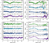 |
Fig. 7. Residuals of the N2 flux-resolved spectra (FPMA in gray; FPMB in varying colors). The dashed orange lines mark the CRSF positions, using the values listed in Table B.1. Renormalizing the spectral model to the source flux without changing spectral parameters results in the χ2 residuals (a) and ratio (b). Refitting the parameters of the four flux-resolved spectra simultaneously leads to the best fit (c). (d): Contribution of the “10 keV feature”, showing the resulting ratio after removing the component from the best-fit. |
To quantify the change in the 10 keV band, we modeled the flux-resolved spectra with our baseline model. Since foreground absorption is flux-independent on the short timescales considered here and Swift coverage is insufficient (covering fewer than four QPO cycles; see Fig. 3) in our spectral fits, we couple NH across the flux-resolved spectra. Similarly, several other parameters are flux-independent, including the detector constant cFPMB and the coupling constant between the cyclotron line width and energy, cCRSF, σ. As a sanity check, we also performed the following analysis without coupling these constants, with similar principal results. The energy of the “10 keV feature” was also coupled, as initial spectral fits with free E10 keV showed no significant variations. Applying these constraints helped us constrain the remaining spectral parameters, in particular the position of the fundamental CRSF of R1.4, as this dataset has the lowest signal-to-noise ratio among all subsets. The resulting simultaneous fit of all four spectra describes the spectra and their variation well (χ2/d.o.f. = 1429.2/1220 = 1.17 for N1 and χ2/d.o.f. = 1416.4/1211 = 1.17 for N2). The resulting best-fit parameters are listed in Table B.2 and visualized in Fig. 8. As shown by the residuals in Figs. A.1c and 7c, the model gives a good description of the data. Fitting the datasets individually, instead of simultaneously as mentioned above, leads to comparable parameters within the uncertainties.
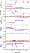 |
Fig. 8. Selected best-fit parameters of the flux-resolved spectra of N1 (red) and N2 (blue), as given in Table B.2. The horizontal bars indicate the band for the rate selection (using the full NuSTAR energy range). The vertical error bars show the 90% confidence interval for the values shown. |
We also attempted spectral fitting with fewer constraints, for example, individually determining cCRSF, σ and E10 keV for each spectral subset. This resulted in fit statistics nearly as good as our final results; however, it produced a physically unreasonable combination of parameters, such as the fundamental CRSF describing an unreasonably high continuum fraction. In particular, the data from the lowest rate band could not be well constrained. Since our previous modeling approach already describes the data well, a more complicated model is not justified. We thus adopted it as our best-fit model.
5.2. The “10 keV feature” as a distinct spectral component
To visualize the overall contribution of the “10 keV feature” to the spectra, in Figs. A.1d and 7d, we show the residuals when setting the flux of the Gaussian component to zero. The residuals clearly show that the feature has a constant width, but that its relative contribution to the remaining continuum decreases with increasing count rate. We note that the energy range affected by the “10 keV feature” also contains the fluorescent iron lines. Since the lines are much narrower than the “10 keV feature”, it is possible to separate the behavior of the fluorescent lines from that of the “10 keV feature”.
Although we can separate the fluorescent lines from the feature, the energy range around ∼10 keV contains contributions from multiple other spectral components, such as the fundamental CRSF. Degeneracies between the parameters describing these features can complicate the interpretation of our fit results. We therefore examine the correlations between these components by looking at the confidence contours for different pairs of parameters, specifically the “10 keV feature”, fundamental CRSF, and cutoff power-law continuum (Lampton et al. 1976).
Figure 9 shows the confidence regions between the relative flux of the “10 keV feature”, i.e., the ratio of the flux to the “10 keV feature” and the 3–50 keV cutoff power-law flux, F10 keV/FPL, and the centroid energy of the “10 keV feature” E10 keV. The relative flux of the “10 keV feature” with respect to the continuum flux increases as continuum flux decreases, leading to separated solutions. Using the approach outlined by Ferrigno et al. (2020), which computes the distribution of correlation coefficients between two variables assuming the posterior intervals have Gaussian distributions, we find that the false alarm probability for the correlation between F10 keV/FPL and FPL is 0.11 for N1 and 0.05 for N2. The corresponding r2 values are [0.82, 0.89, 0.94] (N1) and [0.93, 0.95, 0.97] (N2).
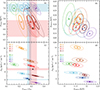 |
Fig. 9. Confidence contours of ratios between fundamental CRSF parameters, “10 keV feature”, and continuum flux correlations. For all flux-resolved spectra, the best-fit values are marked with a cross. The dotted lines show the 3σ contours, and the solid lines indicate the 1σ contours for the N1 (red) and N2 (blue) observations, respectively. The black points mark the best-fit values from the flux-averaged dataset, while the shaded regions in the left panels (N1 in red and N2 in blue) highlight the uncertainties of the averaged best fit, as given in Table B.1. |
We emphasize that our fits coupled E10 keV across the rate bands, since initial fits showed no indication count-rate dependence on the feature’s center energy. We also emphasize that E10 keV changed between the two observations.
Again using confidence contours, we checked for possible correlations between the CRSF and continuum parameters (Fig. 9b and d). The data are described using the same value for cCRSF, 0 for all resolved spectra of an observation (Table B.2). For observation N1, Fig. 9b shows no visible changes in the CRSF parameters DCRSF, 0 and ECRSF, 0. We note a minor anticorrelation in the N2 analysis, but all values for DCRSF, 0 still agree within 3σ and provide no evidence of flux-dependent variability, while ECRSF, 0 only varies slightly. Figures 9c and d clearly show FPL increasing with count rate across the selected bands of both observations, enabling us to probe the behavior of the “10 keV feature” at different luminosities.
6. Discussion
In the following we discuss the interplay between the source’s CRSFs, its “10 keV feature” (Sect. 6.1), and their parameter changes between datasets (Sect. 6.2). We conclude this section by giving an overview of possible origins of the “10 keV feature” (Sect. 6.3).
6.1. Disentangling the “10 keV feature” and the CRSFs
As shown in Sect. 5, the flux-averaged model still provides a rather good description of the spectral shape below ∼6 keV and above ∼20 keV after renormalization (Fig. 7a). A separate spectral component, with a different flux-dependent behavior than that of the underlying continuum, must contribute to the emission at around 10 keV.
Apart from the power-law continuum, the spectrum around 10 keV is shaped by two spectral components, the fundamental CRSF and the “10 keV feature”. We can assess fundamental cyclotron line variability based on the behavior of the higher harmonics, which are easier to decouple from the continuum. To investigate these changes, we look at the data-model ratios of the spectral subsets, using the rescaled flux-averaged model. Apart from the strong deviation around ∼10 keV, we find further variations at higher energies that are less statistically significant (see Figs. A.1a and 7a). Although these deviations seem to appear where the higher harmonic CRSFs are located, they do not exactly align with the harmonic energies. Furthermore, the residuals around 10 keV can be resolved after refitting, while higher-energy wiggles remain visible (see Figures A.1c and 7c). This speaks against a systematic shift in the cyclotron energy or in the strength of the higher harmonics. Moreover, variability of the cyclotron energy with count rate (Fig. 9d) is only visible for the N2 observation, not in the N1 data, and is therefore unlikely to be the cause of the flux-dependence seen in both observations.
We conclude that even if the cyclotron line is slightly variable, this variability is not sufficiently strong to describe the observed flux changes in the 10 keV band. This is further supported by the failure of attempts to model the rate-dependent flux change in the ∼10 keV region solely by varying the CRSF parameters and keeping both the “10 keV feature” and the continuum fixed. This leaves only the “10 keV feature” as the source of the observed flux-dependence.
6.2. Flux-correlations of the “10 keV feature” within and between observations
In the following we examine the changes in the “10 keV feature” parameters. First, the confidence contours shown in Fig. 9c again support our main result that within each observation the flux ratio F10 keV/FPL is strongly anticorrelated with the overall continuum FPL. This is the first time that this flux-dependent variation in the 4U 0115+63 spectra is reported. In previous analyses, when comparing multiple observations from the same or several outbursts, the change in the spectra was not seen. It might be that this independent behavior of the “10 keV feature” only occurs on shorter timescales comparable with luminosity changes in the ∼500 s QPOs. Overall, these results again hint toward the “10 keV feature” being an additional spectral component. This correlation is strongest in the lower-luminosity observation N2. There is a similar trend between FPL and the cyclotron line energy ECRSF, 0, with a more apparent anticorrelation for the N2 observation (Fig. 9d). The similarity between the two observed correlations may point to a common origin.
However, while we do not observe any dependence of the “10 keV feature” energy on the individual rate bands within each observation, we do find that the centroid energy differs between the two observations, with the more luminous observation N1 showing a lower energy for the “10 keV feature”. This trend between observations is consistent with M13, who suggested that the centroid energy decreases with increasing overall flux. Similarly, we find a small variation in the feature’s width and no change in the CRSF energy between the two observations. Such a shift in the “10 keV feature” between observations could hint at an additional luminosity dependence of its underlying creation mechanism. This diverging behavior for the “10 keV feature” energy and cyclotron line rather suggests unrelated underlying physical mechanisms, in contrast to the similar rate dependence seen within each observation.
6.3. Possible physical origin of the “10 keV feature”
Our results, particularly the anticorrelation between the flux ratio F10 keV/FPL and the power-law flux presented in Sect. 5, support the interpretation that the “10 keV feature” represents a spectral component that is to some degree different in its formation from the overall continuum. However, this decoupling is not complete, as the flux of the “10 keV feature” still increases with the power-law flux, suggesting that the “10 keV feature” likely originates from the same physical environment. Based on our current understanding of spectral formation in highly magnetized plasma near the NS surface, several possible explanations for the origin of this feature can be outlined. Here, we review the proposed physical mechanisms for the formation of the spectrum at intermediate energies – and, more specifically, the “10 keV feature”– and present our interpretations with respect to the observed behavior.
The X-ray continuum in the accretion channel is expected to form by thermal and bulk Comptonization of bremsstrahlung, blackbody radiation, and cyclotron emission (see, for example, Mészáros 1992; Arons et al. 1987). Cyclotron emission occurs when collisions between electrons and protons in a magnetized plasma excite electrons to higher Landau levels. Excitations are followed by radiative decay, producing photons with energies approximately equal to the local cyclotron energy. When collisions occur due to the thermal motion of particles, this process is known as cyclotron cooling. When the cyclotron energy is comparable to the plasma temperature, it can become the dominant cooling mechanism. Depending on reprocessing of cyclotron photons by the surrounding plasma, they can significantly contribute to the total flux. It is important to note, however, that generally all radiative processes, including bremsstrahlung and Compton scattering are affected by the strong magnetic field, which introduces anisotropy, resonances, and polarization effects.
The physical models currently available for fitting the spectra of X-ray pulsars are limited to continuum models that describe polarization- and angle-averaged bulk and thermal Comptonization of seed bremsstrahlung, blackbody, and cyclotron photons (Becker & Wolff 2007; Farinelli et al. 2016). In these models, bremsstrahlung is assumed to follow the classical, nonmagnetic cross section, while cyclotron emission accounts for magnetic effects. Such continuum models typically provide a smooth power-law-like spectrum with a high-energy cutoff dominated by the Comptonized bremsstrahlung (see, e.g., Becker & Wolff 2007). Ferrigno et al. (2009) adopted the Becker & Wolff (2007) model to fit BeppoSAX data of the 1999 outburst of 4U 0115+63. While their phenomenological model required significant contribution from the “10 keV feature” to the total flux, the physical model was able to describe the spectra with only a minor Gaussian component at ∼9 keV to flatten the residuals. At the same time, the continuum formation in the model was dominated by cyclotron emission. This was possible, however, only by assuming a magnetic field for the cyclotron emission almost twice as low as that estimated from the observed fundamental cyclotron resonance. Ferrigno et al. (2009) interpreted this discrepancy as possible evidence for a spatial separation between the region where the cyclotron emission is produced and the region where the cyclotron lines are imprinted onto the spectrum. In this case, the cyclotron emission would originate higher up in the accretion channel and then be advected downward by the bulk flow, reprocessed by the thermal plasma, and emitted from the column walls where CRSFs form. See Becker & Wolff (2022) and Li et al. (2024) for further extensions of this model and West et al. (2017a); West et al. (2017b); West et al. (2024) for a discussion of a variant of this model where the height-dependent structure is solved using a numerical approach.
We note, however, that Becker & Wolff (2007) assume the seed photons are mainly thermal cyclotron emission (in addition to those from bremsstrahlung and blackbody radiation), which is unlikely to dominate under conditions where the bulk flow velocity remains high and capable of advecting photons downward. At the same time, under conditions typical for accretion columns in X-ray pulsars, cyclotron processes resulting from thermal collisions must be treated as part of the bremsstrahlung emissivity and free-free absorption, which reduces their contribution and influences spectral formation (see Nagel 1980; Nagel & Ventura 1983; Meszaros & Nagel 1985a). This fact, along with the lack of bulk-induced cyclotron emission, prevents a reliable assessment of the true contribution of cyclotron emission using the currently available continuum models.
B20 suggested that for conditions where the cyclotron energy is close to the local plasma temperature, as expected for 4U 0115+63’s relatively low magnetic field, cyclotron emission from thermal collisions could result in a broad, emission line-like excess. The position of this feature would depend on the plasma temperature and the cyclotron energy. A similar effect has been proposed for nonthermal (bulk-induced) collisions between ambient electrons in the accretion channel and the bulk flow (Nelson et al. 1993). Simulations by Nelson et al. (1995) showed that this effect can result in the formation of a broad line-like excess in the spectrum. However, the formation of this feature depends on the energy deposition within the emitting region. For bulk-flow collisions, simulations show that collisional excitations mainly occur in the upper (though optically thick) part of the NS atmosphere (see, for example, Miller et al. 1989). Assessing the efficiency and the exact signatures of thermal-motion-induced excitations also requires a simultaneous treatment of the energy balance in the emission region and radiative transfer.
Other possible explanations for the “10 keV feature” are based on the fact that spectral formation must include strong polarization effects and radiation redistribution in a hot plasma, and that the formation of the continuum and cyclotron lines cannot be fully decoupled. Together, these effects provide a complex continuum shape characterized by dips and excesses imposed on a general power-law cutoff (Sokolova-Lapa et al. 2023). Depending on the magnetic field strength and local plasma conditions, several basic mechanisms for the formation of a “10 keV feature”-like hump at intermediate energies can be outlined. First of all, in a strong magnetic field the two polarization modes of radiation have principally different energy- and angle-dependent opacities. This behavior is imprinted onto the radiation emerging from a strongly magnetized medium, leading to characteristic energy-dependent structures in the two polarization modes (see, for example, Nagel 1981; Meszaros & Nagel 1985a), which can, in principle, be visible even in the polarization-averaged spectrum. Under typical conditions, the spectrum of the extraordinary mode generally peaks at intermediate energies, around ∼10 keV, and could therefore be responsible for the “10 keV feature” (Sokolova-Lapa et al. 2023). We note that the location of the peak varies only mildly with magnetic field strength (Sokolova-Lapa 2023). This scenario for the formation of the hump could in principle be tested observationally with X-ray polarimetry.
Another possibility involves a more complex formation of the fundamental line. Since CRSFs arise in spectra due to resonant Compton scattering in a hot plasma, their formation is subject to significant redistribution, which can lead to the development of line wings. At the plasma temperatures typically expected in the accretion channel (4–8 keV) and under sufficiently strong magnetic fields, it is primarily the red wing of the fundamental line that becomes prominent in the spectra (Alexander et al. 1989; Schönherr et al. 2007; Schwarm et al. 2017). Simultaneous treatment of the continuum and cyclotron line formation shows that this broadened red wing can produce a noticeable hump at energies below the fundamental cyclotron resonance (Sokolova-Lapa 2023). Interestingly, cyclotron line formation tends to produce a blue wing for moderate magnetic fields when bulk motion Comptonization is considered (Loudas et al. 2024).
Figure 10 (top) shows an example of spectra in two polarization modes, obtained from radiative transfer simulations in a highly magnetized, warm, steady-state plasma. For this exploratory study, we used the homogeneous model of Meszaros & Nagel (1985a); Meszaros & Nagel (1985b), also utilized by Sokolova-Lapa et al. (2023), calculated with the FINRAD transfer code and magnetic opacities for both the continuum and the fundamental cyclotron resonance. The transfer was performed in a 1D slab geometry, assuming a high Thomson optical depth, τT = 1000 and an electron density, ne = 1022 cm−3. We set the electron temperature to 5 keV and chose a relatively low magnetic field, corresponding to a cyclotron energy of 20 keV on the NS surface.
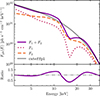 |
Fig. 10. Top: Modeled photon flux in two polarization modes. The figure emphasizes the formation of a strong red wing due to redistribution near cyclotron resonance. Simulations were performed for a homogeneous slab of self-emitting magnetized plasma with τT = 1000, ne = 1022 cm−3, kTe = 5 keV, and Ecyc = 20 keV. The spectra for each polarization mode are integrated over angles. Photon polarization modes, mode 1 (F1) and mode 2 (F2), include vacuum effects and plasma polarization (corresponding to the continuous behavior of the refractive indices, see Sokolova-Lapa et al. 2023, for more details). Assuming a gravitational redshift of (1 + z) = 1.24, the cyclotron line in the final spectrum appears at 15 keV. The spectra are shown on the redshifted energy grid. A fit to the power-law spectrum with a high-energy cutoff (cutoffpl), using a photon index of Γ = 0.47, a cutoff energy of Efold = 6.6 keV, and a normalization of N = 2.4 × 1032, is shown in energy flux space to illustrate the generally assumed continuum behavior. Bottom: Ratio between the modeled photon flux and cutoffpl. |
This setup results in a cyclotron line at ∼16 keV in the redshifted, angle-integrated spectra. The combined spectrum for the polarization modes show a general power-law-like behavior with a high-energy cutoff. However, cyclotron resonance, formed through complex energy and angle redistribution, affects the spectrum over a wide range of energies.
We approximate the modeled spectrum as a power law including a high-energy cutoff (cutoffpl) and show the total flux ratio in Fig. 10 (bottom). Below the resonance, the excess in the form of the cyclotron line’s red wing is particularly noticeable. Note that in reality, for lower magnetic fields, the spectral shape of the line’s blue wing may be influenced by a second harmonic cyclotron line not included in the theoretical model. Although we chose the magnetic field to represent the case of 4U 0115+63, these simulations are not intended to model the spectrum of this particular source. They merely illustrate the complexity of the spectra that emerges even within this simplified framework. These complexities manifest as dip- or hump-like deviations from the power-law continuum. Additional physical effects, such as the influence of bulk motion and light bending near the NS, may further modify the spectra significantly. The deviation of the humps from the continuum, shown in Fig. 10, is of similar order of magnitude to the relative flux of the “10 keV feature” found in our analysis (Figs. A.1d and 7d). It is also compatible with the ∼35% and ∼51% of the continuum flux attributed to the “10 keV feature” in the analysis of earlier observations by B20. We emphasize that we currently do not fully know how changes of plasma parameters affect changes in the accretion flow. Further effects, such as the influence of temperature in the line-forming region on photon reprocessing, have not yet been fully accounted for. These results are therefore exploratory only.
7. Summary and conclusions
In this paper we analyzed short-timescale flux variations in the X-ray spectrum of 4U 0115+63 on timescales of the system’s QPOs and the base-level flux changes. As the flux variations on QPO timescales could be due to changes in the accretion flow, we performed a count-rate-resolved analysis to study the spectral behavior at different intensities. As the individual QPO peaks in the light curve show strong variability (see Fig. 3), this selection does not constitute a QPO phase-resolved analysis. After establishing a model for the flux-averaged datasets (Sect. 4) and then applying it to the flux-resolved analysis (Sect. 5.1), we identified a change in the overall spectral shape, particularly in the energy range of the “10 keV feature”, compared to the flux-averaged data. This suggests the “10 keV feature” is an independent spectral component rather than a modeling artifact.
Assuming an exponentially cutoff power-law continuum, our results provide the strongest evidence to date that the “10 keV feature” is likely a separate spectral component. Specifically, we find that the centroid energy of the “10 keV feature” is flux-independent (Fig. 9a) within each individual observation, while its relative flux, F10 keV/FPL, depends on flux (Fig. 9c). Since flux-dependent changes in the CRSFs do not affect the “10 keV feature” (Fig. 9b), these results strengthen the interpretation of the “10 keV feature” as a separate spectral component and allows us to explain the spectrum without using a second fundamental CRSF, as sometimes done in the literature. Although both observations show similar principal behavior, E10 keV differs between them, potentially due to the different source fluxes. If true, this result could suggest some level of coupling between the physical formation of the general continuum and the “10 keV feature”.
As discussed in Sect. 6.3, there are three possible explanations for the “10 keV feature”. First, as speculated by B20, the “10 keV feature” could be due to cyclotron emission. Second, a more complex formation mechanism for the CRSFs, in which Compton scattering produces a broadened red wing of the absorption line, could mimic the feature. Finally, polarized radiative transfer that accounts for cyclotron resonance redistribution in strongly magnetized plasmas also yields a spectral feature in the 10 keV band (Sokolova-Lapa et al. 2023). Further observations, especially with X-ray polarimetry above ∼7 keV – that is, at harder energies than those with current missions such as IXPE – would help us choose between these possibilities.
Acknowledgments
We thank the XMAG collaboration for all the helpful discussions. This work has been partly funded by DLR under grants 50 QR 2103 and 50 OR 2410, and by the eROSTEP research unit (WI 1860/17-2). The material is based on work supported by NASA under award number 80GSFC21M0002 and award number 80GSFC21M0006. This research has made use of ISIS functions (ISISscripts) provided by ECAP/Remeis observatory and MIT (http://www.sternwarte.uni-erlangen.de/isis/). This research has made use of data and/or software provided by the High Energy Astrophysics Science Archive Research Center (HEASARC), which is a service of the Astrophysics Science Division at NASA/GSFC. This research has made use of data from the NuSTAR mission, a project led by the California Institute of Technology, managed by the Jet Propulsion Laboratory, and funded by the National Aeronautics and Space Administration. Data analysis was performed using the NuSTAR Data Analysis Software (NuSTARDAS), jointly developed by the ASI Science Data Center (SSDC, Italy) and the California Institute of Technology (USA). We acknowledge the use of public data from the Swift data archive. This work has made use of data from the European Space Agency (ESA) mission Gaia (https://www.cosmos.esa.int/gaia), processed by the Gaia Data Processing and Analysis Consortium (DPAC, https://www.cosmos.esa.int/web/gaia/dpac/consortium). Funding for the DPAC has been provided by national institutions, in particular the institutions participating in the Gaia Multilateral Agreement.
References
- Alexander, S. G., Meszaros, P., & Bussard, R. W. 1989, ApJ, 342, 928 [Google Scholar]
- Arnaud, K., Gordon, C., & Dorman, B. 2022, Xspec – An X-Ray Spectral Fitting Package, https://heasarc.gsfc.nasa.gov/xanadu/xspec/manual/XspecManual.html, accessed on 2022-09-21 [Google Scholar]
- Arons, J., Klein, R. I., & Lea, S. M. 1987, ApJ, 312, 666 [Google Scholar]
- Bachetti, M., & Huppenkothen, D. 2018, ApJ, 853, L21 [Google Scholar]
- Bachetti, M., Harrison, F. A., Cook, R., et al. 2015, ApJ, 800, 109 [NASA ADS] [CrossRef] [Google Scholar]
- Bailer-Jones, C. A. L., Rybizki, J., Fouesneau, M., Demleitner, M., & Andrae, R. 2021, AJ, 161, 147 [Google Scholar]
- Barthelmy, S. D., Barbier, L. M., Cummings, J. R., et al. 2005, Space Sci. Rev., 120, 143 [Google Scholar]
- Becker, P. A., & Wolff, M. T. 2007, ApJ, 654, 435 [NASA ADS] [CrossRef] [Google Scholar]
- Becker, P. A., & Wolff, M. T. 2022, ApJ, 939, 67 [NASA ADS] [CrossRef] [Google Scholar]
- Berger, K. 2022, MSc Thesis, Friedrich-Alexander-Universität Erlangen-Nürnberg [Google Scholar]
- Bissinger né Kühnel, M., Kreykenbohm, I., Ferrigno, C., et al. 2020, A&A, 634, A99 [NASA ADS] [CrossRef] [EDP Sciences] [Google Scholar]
- Burrows, D. N., Hill, J. E., Nousek, J. A., et al. 2005, Space Sci. Rev., 120, 165 [Google Scholar]
- Coburn, W., Heindl, W. A., Rothschild, R. E., et al. 2002, ApJ, 580, 394 [NASA ADS] [CrossRef] [Google Scholar]
- Cominsky, L., Clark, G. W., Li, F., Mayer, W., & Rappaport, S. 1978, Nature, 273, 367 [NASA ADS] [CrossRef] [Google Scholar]
- Diez, C. M., Grinberg, V., Fürst, F., et al. 2022, A&A, 660, A19 [NASA ADS] [CrossRef] [EDP Sciences] [Google Scholar]
- Ding, Y. Z., Wang, W., Zhang, P., et al. 2021, MNRAS, 503, 6045 [Google Scholar]
- Dugair, M. R., Jaisawal, G. K., Naik, S., & Jaaffrey, S. N. A. 2013, MNRAS, 434, 2458 [Google Scholar]
- Farinelli, R., Ferrigno, C., Bozzo, E., & Becker, P. A. 2016, A&A, 591, A29 [NASA ADS] [CrossRef] [EDP Sciences] [Google Scholar]
- Ferrigno, C., Becker, P. A., Segreto, A., Mineo, T., & Santangelo, A. 2009, A&A, 498, 825 [NASA ADS] [CrossRef] [EDP Sciences] [Google Scholar]
- Ferrigno, C., Bozzo, E., & Romano, P. 2020, A&A, 642, A73 [NASA ADS] [CrossRef] [EDP Sciences] [Google Scholar]
- Fürst, F., Kreykenbohm, I., Pottschmidt, K., et al. 2010, A&A, 519, A37 [CrossRef] [EDP Sciences] [Google Scholar]
- Fürst, F., Pottschmidt, K., Wilms, J., et al. 2014, ApJ, 780, 133 [Google Scholar]
- Gaia Collaboration (Prusti, T., et al.) 2016, A&A, 595, A1 [NASA ADS] [CrossRef] [EDP Sciences] [Google Scholar]
- Gaia Collaboration (Vallenari, A., et al.) 2023, A&A, 674, A1 [NASA ADS] [CrossRef] [EDP Sciences] [Google Scholar]
- Gehrels, N.& Swift Team 2004, New A Rev., 48, 431 [Google Scholar]
- Giacconi, R., Murray, S., Gursky, H., et al. 1972, ApJ, 178, 281 [NASA ADS] [CrossRef] [Google Scholar]
- Harrison, F. A., Craig, W. W., Christensen, F. E., et al. 2013, ApJ, 770, 103 [Google Scholar]
- Heindl, W. A., Coburn, W., Gruber, D. E., et al. 1999, ApJ, 521, L49 [NASA ADS] [CrossRef] [Google Scholar]
- Heindl, W. A., Coburn, W., Gruber, D. E., et al. 2000, BAAS, 32, 1230 [Google Scholar]
- Houck, J. C., & Denicola, L. A. 2000, ASP Conf. Ser., 216, 591 [Google Scholar]
- Iyer, N., Mukherjee, D., Dewangan, G. C., Bhattacharya, D., & Seetha, S. 2015, MNRAS, 454, 741 [NASA ADS] [CrossRef] [Google Scholar]
- Jain, C., Sharma, P., & Dutta, A. 2025, Adv. Space Res., 75, 1490 [Google Scholar]
- Kortright, J. B., & Thompson, A. C. 2000, X-Ray Data Booklet – Section 1.2 X-ray emission energies, https://xdb.lbl.gov/Section1/Sec_1-2.html, accessed on 2021-06-16 [Google Scholar]
- Lampton, M., Margon, B., & Bowyer, S. 1976, ApJ, 208, 177 [Google Scholar]
- Li, J., Wang, W., & Zhao, Y. 2012, MNRAS, 423, 2854 [Google Scholar]
- Li, P. P., Becker, P. A., & Tao, L. 2024, A&A, 689, A316 [NASA ADS] [CrossRef] [EDP Sciences] [Google Scholar]
- Li, P. P., Tao, L., Ma, R. C., et al. 2025, A&A, 703, A124 [NASA ADS] [CrossRef] [EDP Sciences] [Google Scholar]
- Liu, B.-S., Tao, L., Zhang, S.-N., et al. 2020, ApJ, 900, 41 [NASA ADS] [CrossRef] [Google Scholar]
- Loudas, N., Kylafis, N. D., & Trümper, J. 2024, A&A, 685, A95 [NASA ADS] [CrossRef] [EDP Sciences] [Google Scholar]
- Madsen, K. K., Beardmore, A., & Page, K. 2020, X-calibration of NuSTAR and Swift, https://iachec.org/wp-content/presentations/2020/Xcal_swift_nustar.pdf [Google Scholar]
- Madsen, K. K., Burwitz, V., Forster, K., et al. 2021, arXiv e-prints [arXiv:2111.01613] [Google Scholar]
- Manikantan, H., Paul, B., & Rana, V. 2023, MNRAS, 526, 1 [Google Scholar]
- Manikantan, H., Paul, B., Sharma, R., Pradhan, P., & Rana, V. 2024, MNRAS, 531, 530 [Google Scholar]
- Martin, R. G., & Charles, P. A. 2024, MNRAS, 528, L59 [Google Scholar]
- Martin, R. G., Nixon, C., Armitage, P. J., Lubow, S. H., & Price, D. J. 2014, ApJ, 790, L34 [Google Scholar]
- Mészáros, P. 1992, High-Energy Radiation from Magnetized Neutron Stars (Chicago: Univ. Chicago Press) [Google Scholar]
- Meszaros, P., & Nagel, W. 1985a, ApJ, 298, 147 [NASA ADS] [CrossRef] [Google Scholar]
- Meszaros, P., & Nagel, W. 1985b, ApJ, 299, 138 [NASA ADS] [CrossRef] [Google Scholar]
- Miller, G., Wasserman, I., & Salpeter, E. E. 1989, ApJ, 346, 405 [Google Scholar]
- Miyamoto, S., Kimura, K., Kitamoto, S., Dotani, T., & Ebisawa, K. 1991, ApJ, 383, 784 [NASA ADS] [CrossRef] [Google Scholar]
- Müller, S., Ferrigno, C., Kühnel, M., et al. 2013, A&A, 551, A6 [NASA ADS] [CrossRef] [EDP Sciences] [Google Scholar]
- Nagel, W. 1980, ApJ, 236, 904 [Google Scholar]
- Nagel, W. 1981, ApJ, 251, 278 [NASA ADS] [CrossRef] [Google Scholar]
- Nagel, W., & Ventura, J. 1983, A&A, 118, 66 [NASA ADS] [Google Scholar]
- Nakajima, M., Mihara, T., Makishima, K., & Niko, H. 2006, ApJ, 646, 1125 [CrossRef] [Google Scholar]
- Negueruela, I., & Okazaki, A. T. 2001, A&A, 369, 108 [NASA ADS] [CrossRef] [EDP Sciences] [Google Scholar]
- Nelson, R. W., Salpeter, E. E., & Wasserman, I. 1993, ApJ, 418, 874 [Google Scholar]
- Nelson, R. W., Wang, J. C. L., Salpeter, E. E., & Wasserman, I. 1995, ApJ, 438, L99 [Google Scholar]
- Okazaki, A. T., Hayasaki, K., & Moritani, Y. 2013, PASJ, 65, 41 [NASA ADS] [Google Scholar]
- Pottschmidt, K., Kreykenbohm, I., Wilms, J., et al. 2005, ApJ, 634, L97 [NASA ADS] [CrossRef] [Google Scholar]
- Rappaport, S., Clark, G. W., Cominsky, L., Joss, P. C., & Li, F. 1978, ApJ, 224, L1 [NASA ADS] [CrossRef] [Google Scholar]
- Rouco Escorial, A., Bak Nielsen, A. S., Wijnands, R., et al. 2017, MNRAS, 472, 1802 [NASA ADS] [CrossRef] [Google Scholar]
- Roy, J., Agrawal, P. C., Iyer, N. K., et al. 2019, ApJ, 872, 33 [Google Scholar]
- Roy, K., Manikantan, H., & Paul, B. 2024, A&A, 690, A50 [NASA ADS] [CrossRef] [EDP Sciences] [Google Scholar]
- Santangelo, A., Segreto, A., Giarrusso, S., et al. 1999, ApJ, 523, L85 [NASA ADS] [CrossRef] [Google Scholar]
- Schönherr, G., Wilms, J., Kretschmar, P., et al. 2007, A&A, 472, 353 [NASA ADS] [CrossRef] [EDP Sciences] [Google Scholar]
- Schwarm, F. W., Schönherr, G., Falkner, S., et al. 2017, A&A, 597, A3 [NASA ADS] [CrossRef] [EDP Sciences] [Google Scholar]
- Sokolova-Lapa, E. 2023, Ph.D. Thesis, Friedrich-Alexander-Universität Erlangen-Nürnberg [Google Scholar]
- Sokolova-Lapa, E., Stierhof, J., Dauser, T., & Wilms, J. 2023, A&A, 674, L2 [NASA ADS] [CrossRef] [EDP Sciences] [Google Scholar]
- Staubert, R., Trümper, J., Kendziorra, E., et al. 2019, A&A, 622, A61 [NASA ADS] [CrossRef] [EDP Sciences] [Google Scholar]
- Stierhof, J. J. R., Sokolova-Lapa, E., Berger, K., et al. 2025, A&A, 698, A308 [NASA ADS] [CrossRef] [EDP Sciences] [Google Scholar]
- Thalhammer, P., Bissinger, M., Ballhausen, R., et al. 2021, A&A, 656, A105 [NASA ADS] [CrossRef] [EDP Sciences] [Google Scholar]
- Troja, E. 2020, The Neil Gehrels Swift Observatory, Technical Handbook, Version 17.0, https://swift.gsfc.nasa.gov/proposals/techappd/swifttav17.pdf, accessed on 2023-08-17 [Google Scholar]
- Tsygankov, S. S., Lutovinov, A. A., Doroshenko, V., et al. 2016, A&A, 593, A16 [NASA ADS] [CrossRef] [EDP Sciences] [Google Scholar]
- Unger, S. J., Roche, P., Negueruela, I., et al. 1998, A&A, 336, 960 [NASA ADS] [Google Scholar]
- Verner, D. A., Ferland, G. J., Korista, K. T., & Yakovlev, D. G. 1996, ApJ, 465, 487 [Google Scholar]
- Vybornov, V., Klochkov, D., Gornostaev, M., et al. 2017, A&A, 601, A126 [NASA ADS] [CrossRef] [EDP Sciences] [Google Scholar]
- West, B. F., Wolfram, K. D., & Becker, P. A. 2017a, ApJ, 835, 129 [NASA ADS] [CrossRef] [Google Scholar]
- West, B. F., Wolfram, K. D., & Becker, P. A. 2017b, ApJ, 835, 130 [NASA ADS] [CrossRef] [Google Scholar]
- West, B. F., Becker, P. A., & Vasilopoulos, G. 2024, ApJ, 966, L5 [Google Scholar]
- Wijnands, R., & Degenaar, N. 2016, MNRAS, 463, L46 [NASA ADS] [CrossRef] [Google Scholar]
- Wilms, J., Allen, A., & McCray, R. 2000, ApJ, 542, 914 [Google Scholar]
Gaia DR3 quotes a geometric distance of ∼7.3 kpc (Gaia Collaboration 2016, 2023).
Appendix A: Additional figures (N1)
In the main body of the paper we showed the results from the flux-resolved analysis of N2, see Fig. 7. The residuals of the analysis of observation N1 are shown here in Figure A.1.
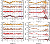 |
Fig. A.1. Residuals of the flux-resolved spectra of N1 (FPMA in gray, FPMB in varying color). The blue dashed lines in panels (a) and (b) mark the positions of the CRSFs, using the values listed in Table B.1. The χ2 residuals (a) and ratio (b), when only evaluating and re-normalizing the flux-averaged best-fit parameters, are shown. Refitting the parameters of the four flux-resolved spectra simultaneously, lead to the best fit as given in panel (c). Panel (d) highlights the contribution of the “10 keV feature”, by showing the resulting ratio after removing the component from the best-fit that is shown in the lower left panel. |
Appendix B: Fit parameters
Table B.1 lists all best fit parameters of the spectral fits to both NuSTAR observations of 4U 0115+63, both with and without considering the corresponding Swift observations. The best fit parameters for the flux-resolved analysis are listed in Table B.2.
Best parameters of the averged spectral fit with confidence limits.
Best parameters of the simultaneous spectral fit of the flux-resolved NuSTAR observations of N1 and N2 with confidence limits.
All Tables
Best parameters of the simultaneous spectral fit of the flux-resolved NuSTAR observations of N1 and N2 with confidence limits.
All Figures
|
Fig. 1. Swift Burst Alert Telescope (BAT; Barthelmy et al. 2005) light curve of the 2015 outburst of 4U 0115+63 in the 15–50 keV band with a binning of 1 d. The blue-shaded regions highlight the quasi-simultaneous NuSTAR and Swift observation times. |
| In the text | |
|
Fig. 2. N1 (top) and N2 (bottom) light curves, using combined data from FPMA and FPMB for clarity binned at three times the spin period of 4U 0115+63. The green-shaded regions highlight the observation periods of the S1 and S2 Swift snapshots. |
| In the text | |
|
Fig. 3. Selected part of the 4U 0115+63 light curve, showing NuSTAR (red) and Swift (dark green) data highlighting the system’s strong QPOs. |
| In the text | |
|
Fig. 4. PSDs of the NuSTAR observations, shown in red for N1 and blue for N2. For comparison the black data points indicate the results obtained by Heindl et al. (1999). The vertical solid orange lines highlight the spin frequency of the NS and its higher harmonics. The vertical dashed lines mark two additional peaks at 1.6 and 2.6 times the NS spin frequency. |
| In the text | |
|
Fig. 5. Selected rates for extracting different flux-resolved spectra from N1 (left) and N2 (right) using 1 s binning. The selection criteria were chosen to be < 700 cts/s, 700–800 cts/s, 800–900 cts/s, and > 900 cts/s for N1 and < 500 cts/s, 500–600 cts/s, 600–700 cts/s, and > 700 cts/s for N2. |
| In the text | |
|
Fig. 6. Top: NuSTAR and Swift spectra of O1 (left) and O2 (right) with the best-fit model (black). The data from XRT are shown in green, FPMA in the lighter color, and FPMB in the darker color. Middle: Visualization of different model components. The data are shown in gray, and the model using the best-fit parameters is shown in black. The component contribution is shown in orange, using a dash-dotted line for the cutoff power law, a dashed line for the “10 keV feature”, and a dotted line for the iron lines. Bottom: Residuals of the best-fit model. |
| In the text | |
|
Fig. 7. Residuals of the N2 flux-resolved spectra (FPMA in gray; FPMB in varying colors). The dashed orange lines mark the CRSF positions, using the values listed in Table B.1. Renormalizing the spectral model to the source flux without changing spectral parameters results in the χ2 residuals (a) and ratio (b). Refitting the parameters of the four flux-resolved spectra simultaneously leads to the best fit (c). (d): Contribution of the “10 keV feature”, showing the resulting ratio after removing the component from the best-fit. |
| In the text | |
|
Fig. 8. Selected best-fit parameters of the flux-resolved spectra of N1 (red) and N2 (blue), as given in Table B.2. The horizontal bars indicate the band for the rate selection (using the full NuSTAR energy range). The vertical error bars show the 90% confidence interval for the values shown. |
| In the text | |
|
Fig. 9. Confidence contours of ratios between fundamental CRSF parameters, “10 keV feature”, and continuum flux correlations. For all flux-resolved spectra, the best-fit values are marked with a cross. The dotted lines show the 3σ contours, and the solid lines indicate the 1σ contours for the N1 (red) and N2 (blue) observations, respectively. The black points mark the best-fit values from the flux-averaged dataset, while the shaded regions in the left panels (N1 in red and N2 in blue) highlight the uncertainties of the averaged best fit, as given in Table B.1. |
| In the text | |
|
Fig. 10. Top: Modeled photon flux in two polarization modes. The figure emphasizes the formation of a strong red wing due to redistribution near cyclotron resonance. Simulations were performed for a homogeneous slab of self-emitting magnetized plasma with τT = 1000, ne = 1022 cm−3, kTe = 5 keV, and Ecyc = 20 keV. The spectra for each polarization mode are integrated over angles. Photon polarization modes, mode 1 (F1) and mode 2 (F2), include vacuum effects and plasma polarization (corresponding to the continuous behavior of the refractive indices, see Sokolova-Lapa et al. 2023, for more details). Assuming a gravitational redshift of (1 + z) = 1.24, the cyclotron line in the final spectrum appears at 15 keV. The spectra are shown on the redshifted energy grid. A fit to the power-law spectrum with a high-energy cutoff (cutoffpl), using a photon index of Γ = 0.47, a cutoff energy of Efold = 6.6 keV, and a normalization of N = 2.4 × 1032, is shown in energy flux space to illustrate the generally assumed continuum behavior. Bottom: Ratio between the modeled photon flux and cutoffpl. |
| In the text | |
|
Fig. A.1. Residuals of the flux-resolved spectra of N1 (FPMA in gray, FPMB in varying color). The blue dashed lines in panels (a) and (b) mark the positions of the CRSFs, using the values listed in Table B.1. The χ2 residuals (a) and ratio (b), when only evaluating and re-normalizing the flux-averaged best-fit parameters, are shown. Refitting the parameters of the four flux-resolved spectra simultaneously, lead to the best fit as given in panel (c). Panel (d) highlights the contribution of the “10 keV feature”, by showing the resulting ratio after removing the component from the best-fit that is shown in the lower left panel. |
| In the text | |
Current usage metrics show cumulative count of Article Views (full-text article views including HTML views, PDF and ePub downloads, according to the available data) and Abstracts Views on Vision4Press platform.
Data correspond to usage on the plateform after 2015. The current usage metrics is available 48-96 hours after online publication and is updated daily on week days.
Initial download of the metrics may take a while.