| Issue |
A&A
Volume 707, March 2026
|
|
|---|---|---|
| Article Number | A336 | |
| Number of page(s) | 17 | |
| Section | Cosmology (including clusters of galaxies) | |
| DOI | https://doi.org/10.1051/0004-6361/202555991 | |
| Published online | 18 March 2026 | |
Gas motion in the intracluster medium of the Virgo cluster replica
1
Université Paris-Saclay, CNRS, Institut d’Astrophysique Spatiale, 91405 Orsay, France
2
INAF, Osservatorio di Astrofisica e Scienza dello Spazio, Via Piero Gobetti 93/3, 40129 Bologna, Italy
3
INFN, Sezione di Bologna, Viale Berti Pichat 6/2, 40127 Bologna, Italy
4
Université de Lille, CNRS, Centrale Lille, UMR 9189 CRIStAL, F-59000 Lille, France
★ Corresponding author: This email address is being protected from spambots. You need JavaScript enabled to view it.
Received:
17
June
2025
Accepted:
19
January
2026
Abstract
Within the deep gravitational potential of galaxy clusters lies the intracluster medium (ICM). At the first order, it is considered to be at hydrostatic equilibrium within the potential well. However, evidence is growing on the observational side and in numerical simulations that the ICM dynamics is non-negligible from an energetic point of view, is mostly turbulent in origin, and provides non-thermal pressure support to the equilibrium. In this work, we intend to characterise the properties of the velocity field in the ICM of a simulated replica of the Virgo cluster. We first studied the 3D and projected properties of the ICM velocity field by computing its probability density functions (PDFs) and its statistical moments. We then estimated the non-thermal pressure fraction from an effective turbulent Mach number, including the velocity dispersion. We finally computed the velocity structure function (VSF) from projected maps of the sightline velocity. In this paper, we first show that the components of the 3D velocity field and the projected quantities along equivalent sightlines are anisotropic and affected by the accretion of gas from filaments. Then, we compare the mean statistical moments of the 3D velocity field to the mean properties of 100 random projections. We show, in particular, an almost linear relation between the standard deviation estimated from direct simulation outputs and sightline velocity dispersion projections, which are comparable to the line broadening of X-ray atomic lines. However, this linear relation does not hold between the direct simulation outputs and the standard deviation of the sightline velocity projections, which are comparable to the line shift of X-ray atomic lines. We find a non-thermal pressure fraction of around 6% within R500 and 9% within Rvir from sightline velocity dispersion, which is in good agreement with direct simulation outputs. Finally, we show that the VSF might probe the turbulent injection scale of active galactic nucleus (AGN) feedback.
Key words: turbulence / methods: numerical / galaxies: clusters: individual: Virgo
© The Authors 2026
 Open Access article, published by EDP Sciences, under the terms of the Creative Commons Attribution License (https://creativecommons.org/licenses/by/4.0), which permits unrestricted use, distribution, and reproduction in any medium, provided the original work is properly cited.
This article is published in open access under the Subscribe to Open model. This email address is being protected from spambots. You need JavaScript enabled to view it. to support open access publication.
1. Introduction
Initial over-densities accreted matter through cosmic history and formed the current clusters of galaxies, which nowadays constitute the nodes of the cosmic web. Simultaneously, cosmic gas fell into these deep gravitational potential wells and was thus gravitationally heated up to 108 K, forming the intracluster medium (ICM; see Kravtsov & Borgani 2012 for a review). In this context, gravity is considered to be by far the most dominant process in the dynamics of the ICM; we thus usually consider that pressure only comes from gravitational heating, inducing purely thermal pressure. Consequently, the ICM gas is assumed to be at hydrostatic equilibrium, allowing us to derive the mass of clusters from the measure of the ICM pressure via the thermal Sunyaev-Zel’dovich effect (tSZ, Sunyaev & Zeldovich 1972) in the sub-millimetre wavelengths and the measure of the ICM density and temperature via bremsstrahlung (e.g. Sarazin 1986; Ettori et al. 2013) in the X-rays (see e.g. Salvati et al. 2018; Pratt et al. 2019; Aymerich et al. 2024, for mass estimation of clusters and their use as a cosmological probes).
The main source of deviation from hydrostatic equilibrium could be gas dynamics in the ICM (e.g. Rasia et al. 2004), which could contribute significantly, in addition to thermal pressure, to the total pressure support (Nelson et al. 2014). In observations, properties of the velocity field in the ICM can be probed with X-ray spectroscopy, provided there is a sufficient resolution to measure precise line shift and broadening to derive sightline velocity and velocity dispersion (see e.g. Zhuravleva et al. 2012; Simionescu et al. 2019 for a review). On the one hand, the XRISM telescope (XRISM Science Team 2020), replacing the Hitomi telescope (e.g. Hitomi Collaboration 2016, 2018), resolves line shift and broadening, although with a limited spatial resolution with respect to XMM-Newton or Chandra. For instance, low, non-thermal pressure has been measured in the core of the A2029 cluster (XRISM Collaboration 2025a) and in its outskirts (XRISM Collaboration 2025b), but also in Coma (XRISM Collaboration 2025c) and other clusters (all compared in XRISM Collaboration 2025d). On the other hand, a refined analysis of XMM-Newton data permitted the mapping of the velocity field in nearby clusters (e.g. Gatuzz et al. 2022a, 2023a,b, 2024), including the Virgo cluster (Gatuzz et al. 2022b). It allowed the study of statistical properties of the velocity field through the velocity structure function (VSF), although with large uncertainties in the measurement of the velocity due to its lower spectral resolution than XRISM. In the future, the NewAthena telescope (Cruise et al. 2025) will allow both high spatial and spectral resolution.
The quantification of the velocity field properties from observations still relies on simplified assumptions: isotropy, homogeneity, and Gaussianity (see e.g. Gatuzz et al. 2023a). Moreover, turbulence in the core of clusters is not fully understood yet, even though it is a very active research field thanks to simulations (e.g. Norman & Bryan 1999; Nagai et al. 2007; Gaspari & Churazov 2013; Porter et al. 2015; Vazza et al. 2017; Vallés-Pérez et al. 2021; Ayromlou et al. 2024; Groth et al. 2025; Vazza & Brunetti 2026). In particular, the role of accretion and merging shocks (e.g. ZuHone 2011; Iapichino et al. 2011; Nagai et al. 2013), active galactic nucleus feedback (AGN) (e.g. Vazza et al. 2013; Bourne & Sijacki 2017; Sotira et al. 2025), stratification (e.g. Shi et al. 2018; Mohapatra et al. 2020; Simonte et al. 2022; Wang et al. 2023), and multiple phases (e.g. Wang et al. 2021; Mohapatra et al. 2022) have been studied. From an observational standpoint, indirectly quantifying turbulence from density fluctuations was proposed (e.g. Gaspari & Churazov 2013; Zhuravleva et al. 2014); this can be derived from X-ray surface brightness fluctuations (e.g. Churazov et al. 2012; Dupourqué et al. 2023, 2024; Heinrich et al. 2024), pressure fluctuations (e.g. Schuecker et al. 2004; Khatri & Gaspari 2016; Romero et al. 2023, 2024; Adam et al. 2025), or temperature fluctuations (e.g. Lovisari et al. 2024), and thus completes spectroscopic studies. This work therefore aims to thoroughly study the properties of the velocity field in the ICM through simulations, using both 3D direct simulation outputs and projections of the sightline velocity and sightline velocity dispersion.
We took advantage of a state-of-the-art cosmological hydrodynamical simulated replica of the Virgo cluster in its local environment (Sorce et al. 2021) to conduct this study, allowing direct comparison with observations. We first describe the simulation and present projections of the sightline velocity and sightline velocity dispersion in Sect. 2. We study the statistical properties of the 3D velocity field components and projected sightline velocities, via the probability distribution function (PDF) and its statistical moments, in Sect. 3. We then derive the turbulent Mach number and the non-thermal pressure support from 3D and projected quantities in Sect. 4. We finally compute the velocity structure function (VSF) in Sect. 5 before discussing the results in Sect. 6 and concluding in Sect. 7.
2. Methodology
2.1. The Virgo replica simulation
We succinctly present the Virgo replica simulation already used in Lebeau et al. (2024a, b, 2025); for more details, see Sorce et al. (2021). Contrary to previous simulations attempting to reproduce the Virgo cluster (e.g. Hoffman et al. 1980; Li & Gnedin 2014; Moran et al. 2014; Zhu et al. 2014), this replica accounts for its local environment. To create it, the initial conditions of this simulation were obtained by reconstructing the initial density field of the local Universe by applying a reverse Zel’dovich approximation (Doumler et al. 2013) to the position and peculiar velocities of galaxies in the Cosmicflows-2 (Tully et al. 2013) dataset (see Sorce et al. 2016 for details). Sorce et al. (2019) then increased the resolution in the region around Virgo and simulated 200 dark matter (DM) replicas of this cluster within its local environment. Among the realisations, the most representative of the 200, in terms of merging history and average properties regarding the full sample, was reused to run a zoom-in, high-resolution hydrodynamical counterpart (Sorce et al. 2021). Both the DM-only and the hydrodynamical run show a very good agreement with observations (see more details in Sorce et al. 2021; Lebeau et al. 2024a), they notably reproduce Virgo’s local environment well, including the filaments along our observer’s sightline and the group of galaxies falling onto Virgo. It is worth noting that the initial conditions used to produce this Virgo replica have been reused in the joint LOCALIZATION1/SLOW2 project (see e.g. Dolag et al. 2023; Hernández-Martínez et al. 2024, 2026). In reproducing the initial conditions of the local Universe, this so-called backward approach differs from the Bayesian forward approach, used in other projects such as ELUCID (Wang et al. 2014) or SIBELIUS (Sawala et al. 2022), where the initial density field is inferred from the observed density field through a Hamiltonian Markov chain method (see Section 3.2 of Lebeau 2025 for more details and references).
This simulation uses the Planck Collaboration XVI (2014) cosmological parameters; that is, a Hubble constant of H0 = 67.77 km s−1 Mpc−1, a dark-energy density of ΩΛ = 0.693, a total matter density of Ωm = 0.307, a baryonic density of Ωb = 0.048, an amplitude of the matter power spectrum at 8 Mpc h−1, σ8 = 0.829, and a spectral index of ns = 0.961. The adaptive mesh refinement (AMR) hydrodynamical code RAMSES (Teyssier 2002) was used to produce this simulation. Within the 500 Mpc h−1 local Universe box, the zoom region is a 30 Mpc diameter sphere with an effective resolution of 81923 DM particles with a mass of mDM = 3 × 10⁷ M⊙. The finest cell size of the AMR grid is 0.35 kpc. The simulation contains additional sub-grid models for radiative gas cooling and heating, star formation, and kinetic feedback from a type II supernova (SN) and AGN, similar to the Horizon-AGN implementation of Dubois et al. (2014, 2016). Moreover, we improved the AGN feedback model by orienting the jet according to the black-hole spin (see Dubois et al. 2021 for details).
2.2. Projected velocity maps
The rdramses code3 was used to extract the DM particles and gas cell properties from the simulation. The Virgo DM halo and its galaxies were identified by applying the Tweed et al. (2009) halo finder, respectively, to the DM particles and the star particles. In this work, we define the gas as the baryonic component in the simulation cells (as in Lebeau et al. 2024b), in which hydrodynamics equations in the Eulerian formalism are solved; it thus does not include the stars. It is important to note that, for this study, we extracted gas cells up to a resolution of 22.5 kpc at best, meaning that we did not go deeper than this resolution level in the cell tree of the simulation. This choice is motivated by the fact that we will hardly be able to reach a spatial resolution below 20 kpc for most of the clusters observed in the X-rays or sub-millimetre wavelengths, and that below this scale complex microphysics processes become important. In addition, we found almost identical velocity structure functions with twice as many resolved maps (see right panel of Fig. B.1), showing that the chosen resolution is sufficient for the studied gas dynamics. In addition, we restricted our study to ICM cells by applying a temperature cut at T = 107 K (see phase diagram of cosmic gas in e.g. Martizzi et al. 2019; Gouin et al. 2022). We produced projections of the velocity fields following Lebeau et al. (2024a,b, 2025). To mimic what could be derived from X-ray spectra atomic line shifts, we computed the mean velocity of ICM simulation cells along a given sightline in the Virgo rest frame. In other words, the velocity of the DM halo, as found by the halo finder, is subtracted from each cell. This procedure is similar to choosing a reference wavelength, typically that of the brightest cluster galaxy (BCG), to estimate the Doppler shift. The sightline velocity is thus defined as
 (1)
(1)
with qi being the weight. We computed both mass-weighted (MW) projections, i.e. qi = mi, the cell mass, and emission-weighted (EW) projections, i.e. qi = ρi2, which is the squared cell density, as in Roncarelli et al. (2018). We also mimicked the X-ray spectra’s atomic line broadening by integrating the velocity dispersion along the sightline defined as
 (2)
(2)
with qi being the same weightings as for the integrated sightline velocity.
The sightline velocity and velocity dispersion are presented in Figs. 1 and A.1 of Appendix A. From left to right, we show the projections along the x, y, and z simulation box axes. We also show the projection along the cen sightline (as in Lebeau et al. 2024a,b), that is, between Virgo and the centre of the local Universe simulation box in which the Virgo zoom-in region is simulated. It is equivalent to our own observer’s sightline. For both figures, the top row presents the EW projections, and the bottom row presents the MW projections. The projections are 5 Mpc wide and contain 2222 pixels of 22.5 kpc in width.
 |
Fig. 1. Projections of the velocity integrated along the vx, vy, vz and vcen sightlines from left to right. The top (bottom) row presents the EW (MW) maps. The solid, dashed and dotted black circles respectively represent Rvir, R500 and R2500. The colour bar goes from −600 km s−1 (blue), meaning an average gas flow coming from the foreground of Virgo and going away from the observer, to 600 km s−1 (red), meaning, inversely, an average gas flow coming from the background of Virgo and coming toward the observer. |
The sightline velocity projections (see Fig. 1) were built so that the sightline points towards the observer; thus, the redder (the bluer) the pixels, the more positive (negative) the integrated velocity is, meaning that, on average, the gas falls onto Virgo from the background (foreground) in this given sightline. The colour convention follows that of other works on projected sightline velocity of the ICM gas (e.g. Gatuzz et al. 2023a), but it is reversed compared to that usually used in studies of the sightline velocities of galaxies associating red (blue) with redshift (blueshift). We observe that, whatever the weighting method, the vx projection is bimodal with a positive (negative) velocity in the upper (lower) part of the map; this is because Virgo is connected to two filaments feeding gas to Virgo and located in the {x < 0, y > 0} ({x > 0, y < 0}) area of the simulation box (see Fig. 1 of Lebeau et al. 2025). The vy and vz are perpendicular to the filaments, so their projections present a spatially scattered distribution of positive and negative velocities. The vcen projection is dominated by positive velocities given that it is almost aligned with filaments and that the matter flow in the background filament dominates that of the foreground one (see also Fig. 1 of Lebeau et al. 2025). We also note that the EW maps are more contrasted than their MW counterparts; the former enhances the denser regions when the latter shows a smoother distribution, which induces differences in the statistical-moment values of their respective velocity fields, as we show later.
3. Statistical properties of the velocity field
In this section, we study the statistical properties of the velocity field. We first analyse the probability distribution functions and their moments for both the 3D velocity field and the four projections presented above. To sample different configurations using a single simulated cluster, we also considered 100 randomly oriented projections.
As a first approximation, we expect that the dynamics in the ICM are only due to the orbital motion inside the gravitational potential well of the cluster. Thus, the PDFs of the velocity field are expected to follow a zero-centred Gaussian distribution in the cluster’s rest frame. This should be the case for the 3D velocity field, but also for projected sightline velocities if there are no projection effects. We also expect isotropy; i.e. the three components of the velocity field should follow a similar distribution, including higher order statistics. Finally, if the velocity field is homogeneous, it should have a similar distribution, whatever the selected cluster region, provided the latter is large enough to be statistically representative.
3.1. 3D PDFs
We first studied the properties of the 3D velocity field by computing the PDFs of the three components of the velocity field within Rvir = 2147 kpc, R500 = 1087 kpc, and R2500 = 515 kpc. These are presented in Fig. 2. Moreover, we calculated the following mass-weighted statistical properties: median, mean (μ), standard deviation (σ), skewness, and kurtosis. They are reported in the top left of Table C.1. A median different from the mean shows that the distribution is asymmetric, and a positive (negative) skewness indicates that there is more weight in the right (left) tail of the distribution, which means more positive (negative) velocities in our case. The kurtosis indicates the flatness or peakedness; a positive (negative) value indicates a flattened (peaked) distribution with more (less) weight in the tails compared to a Gaussian distribution. To compare with the statistical moments and visualise the distributions better, we fitted the PDFs to a Gaussian law, similarly to Gatuzz et al. (2023a). The best-fit values are reported on the top right of Table C.1, and the Gaussian envelopes are displayed as solid black curves in Fig. 2.
 |
Fig. 2. PDFs of the three components of the velocity field within Rvir = 2147 kpc, R500 = 1087 kpc, and R2500 = 515 kpc. The first three rows display the PDFs computed within spheres of decreasing radius from top to bottom. The first three columns display the PDF of each component of the velocity field, vx, from red to yellow, vy in shades of blue, and vz in shades of green, from left to right. The right column overlays the PDFs of the three velocity-field components in a given sphere, and the bottom row overlays the PDFs of a given velocity-field component inside the different spheres. Fitted Gaussian envelopes are displayed as solid black curves. The statistical moments of the PDFs and the best-fit values of the Gaussian fit can be found in Table C.1. |
We first observe that, whatever the component and the sphere radius, the distributions are all roughly centred on zero. Although they are slightly shifted negatively, particularly for the vy and vz components within R2500. μ varies between −118.3 and 2.4 km s−1 most when the velocities are distributed in the [−1000, 1000] km s−1 range and σ is scattered around 250 km s−1. Then, on the one hand, we note that the PDF of the vx component within Rvir and R500 has a lot of weight in the tails, as shown by its high kurtosis. It is due to two filaments, almost aligned with the x-axis of the simulation box (see Fig. 1 of Lebeau et al. 2025), that funnel gas at high velocity towards the cluster. This gas being accreted is certainly not yet thermalised within Virgo’s potential well. It also induces the highest velocity dispersion among the 3D PDFs: 325.6 km s−1. Indeed, the Gaussian fit yields a much smaller value of σ = 265.0 ± 11.1 km s−1. On the other hand, the PDFs of the vy and vz components are tighter, but with a bit more weight in their right tail within Rvir, as probed by their positive skewness. And, inversely, a bit more weight is in the left tail for the vy component within R500. For these three PDFs, the fitted velocity dispersion is lower than that directly estimated from the PDFs, which is expected given their deviation from Gaussianity. Only the PDF of the vz component within R500 shows an almost Gaussian distribution, with close-to-zero skewness and kurtosis and a fitted velocity dispersion in agreement with that of the PDF.
When comparing the PDFs of a component within different radii (bottom row of Fig. 2), we observe a narrowing of the distribution when reducing the radius of the sphere. In particular, within R2500, the tails are less populated. This may be because there is less non-thermal gas motion in the cluster core, even though this Virgo replica is known to be unrelaxed and hosting an active AGN in its core with a growing accretion shock (see Lebeau et al. 2024a). This sphere might also be too small to characterise all the scales of the velocity field. We finally compare the PDFs of the different components within the same sphere. This confirms that, within Rvir, the velocity field is not isotropic because of the high-velocity gas accretion from the cluster’s outskirts. On the contrary, the velocity field seems relatively isotropic within R2500, with quite similar PDFs for the three components. However, it might not be representative of the velocity field in the ICM. Thus, choosing to study the velocity field within R500 might be an acceptable compromise to recover representative statistical properties of the ICM without them being contaminated by large-scale accretion and biased by possible inhomogeneities or the lack of statistics within a smaller sphere.
3.2. 2D PDFs of four projections
We conducted the same analysis with the PDFs of the projected sightline velocity maps shown in Fig. 1. They are presented in Fig. 3, similarly to the 3D velocity field (see Fig. 2). The statistical moments and the best-fit values of these PDFs are reported in the middle (bottom) part of Table C.1 for the EW (MW) projections.
 |
Fig. 3. 2D PDFs of EW and MW maps computed within circles of the radii Rvir, R500, and R2500 from top to bottom, for the vx, vy, vz, and vcen projected velocities from left to right. The PDFs extracted from the EW maps are displayed following the same colour-code as Fig. 2. The fitted Gaussian envelope is also shown as a solid black curve, and a vertical dashed black line represents the mean of the PDF. In addition, the PDFs extracted from the MW maps, their fitted Gaussian envelope, and their mean are overlaid in grey in the same style as their EW counterpart. |
We first examine the mean and the median values; the PDFs of the EW and MW projections are close for each case, except for the vcen projection and especially within R2500. However, they are, overall, more scattered than for the 3D PDFs. As shown by the visual inspection of Fig. 1 conducted in Sect. 2, the vx projection is bimodal due to the gas accreted from two opposite filaments, leading to the largest dispersion among the projections. Then, the vy and vz projections are relatively zero-centred and have smaller dispersions. The vcen projection is dominated by positive velocities due to the alignment with the filaments and the higher gas accretion from the background filament. The mean is about 150 (90) km s−1 for the EW (MW) projections, whatever circle the PDFs are estimated in.
We also notice that, regardless of the projection, the weighting method, and the circle radius, the 2D PDFs are tighter than their 3D counterpart. Their standard deviation is roughly 100 km s−1 or more smaller for both the computed and the best-fit value. Moreover, we observe that the PDFs of the MW projections have much less weight in the tails than their EW counterparts, which is expected given that the MW method tends to smooth the projections when the EW method enhances the density peaks and thus the massive objects potentially falling faster onto Virgo than the overall gas flow. Consequently, the standard deviation is slightly smaller for the MW projections, except for the vx projection within Rvir. Accordingly, the kurtosis is also smaller for the MW projections for most cases.
There are also strong deviations from Gaussianity for the EW projection, in particular for the vx and vz projections within Rvir, and the vcen projection within Rvir and R500. For the vz projection, it is because of a very high velocity and density region on the upper left of the map. It is certainly the gas accreted from the background filament reaching its highest velocity due to gravitational attraction just before being shocked when entering the cluster (as seen in Fig. 1 of Lebeau et al. 2025). For the vx and vcen projections, the important weight in the tails of their PDFs is also due to dense regions enhanced by the EW method, which are certainly halos falling onto Virgo.
In conclusion, there are important projection effects on the sightline velocity projections, particularly for the vx and vcen projections, because of filaments along the sightline. More importantly, they do not have the same statistical properties as their 3D counterparts, particularly the standard deviation.
3.3. Generalisation to 100 randomly oriented projections
We then generalised our method for 100 projections along random sightlines, as was done in Lebeau et al. (2024b). Figure 4 compares the mean statistical properties of the components of the 3D velocity field in the x-axis, and those of the 100 random projections are on the y-axis. From left to right, the median, mean, standard deviation, skewness and kurtosis are displayed. Along the x-axis and y-axis, the error bars are, respectively, the dispersion over the three components of the 3D velocity field and over the 100 projections. To test correlations between data points, we ran a bootstrap sampling. The histogram of the mean values of the sub-samples for each statistical moment and radius shows a central value in very good agreement with the values presented in Fig. 4, and the dispersion is largely within the error bars presented in Fig. 4.
 |
Fig. 4. Comparison of statistical properties of the 3D velocity field (x-axis) over projected sightline velocities (y-axis). We show the mean value and the standard deviation among the three components of the 3D velocity field, i.e. vx, vy, vz, in the x-axis, and among 100 random projections in the y-axis. From left to right, we present the median, the mean, the standard deviation (≡σproj in the top panel of Fig. 5), the skewness, and the kurtosis. We display the quantities estimated from EW (MW) projections within R2500 in orange (cyan), R500 in red (blue), and Rvir in dark red (dark blue). The legend can be found in the central panel. |
We first notice that the median and mean of the projected velocities are scattered around zero; see the first two panels from the left. Their 3D counterparts within R500 and Rvir are close to 0 km s−1, showing that it is almost at rest with respect to the halo velocity, which we consider as Virgo’s rest frame. However, within R2500, the 3D velocity is around −50 km s−1, certainly due to the gas flow triggered by the AGN feedback in Virgo’s core, which is coherent with the large scatter among the projected velocity within this radius. The skewness of the projected velocities is also centred on zero, whatever the radius, with the highest scatter within Rvir being due to the matter accretion from filaments. For the 3D velocity field, it is slightly positive, whatever the radius, meaning that the distribution is slightly asymmetric towards higher velocities. The kurtosis indicates that the larger the radius, the flatter the distribution for both the 3D and the projected velocities. It is due to the accretion at high velocities in the outskirts and the low velocities in the core.
Overall, for these four quantities, the weighting method does not have much impact. On the contrary, we observe a clear trend for the standard deviation: it is higher for EW projections than for MW ones and decreases almost linearly with decreasing radius. More importantly, as written above, it is always smaller than the standard deviation of the ground-truth 3D-simulated velocity field. The one-to-one relation is shown as a dotted diagonal grey line. To investigate this observation in more detail, we computed the ratio of the standard deviation of the sightline velocity projections, named σproj, over the 1D velocity dispersion of the 3D-simulated velocity field, which is the root mean square (rms) of the dispersion of the components:  . The histogram of this ratio over the 100 random projections is presented in the top panel of Fig. 5. The panels present the distributions within R2500, R500, and Rvir from left to right. The distribution of the ratios, and thus the underlying standard deviation, looks relatively Gaussian within the three radii since their mean and median agree well. The histograms confirm that the one hundred sightline velocity projections, both EW and MW, have a smaller velocity dispersion than the ground-truth simulated velocity field, by a factor of around 0.7 for the EW projections and 0.55 for the MW projections, regardless of the radius.
 |
Fig. 5. Histograms of the ratio of the standard deviationof sightline velocity (σproj, top, already presented in central panel of Fig. 4, std stands for standard deviation) and sightline velocity dispersions (σlos, bottom) of one hundred random projections over the 1D velocity dispersion of the 3D velocity field, σsim2 = (σx2 + σy2 + σz2)/3. For each row, we present the ratio of the quantities estimated within R2500 in orange for the EW projections (cyan for MW), R500 in red for the EW projections (blue for MW) and Rvir in dark red for the EW projections (dark blue for MW). The mean (median) of the distributions is displayed as dashed (dotted) vertical lines in the same colours and can be compared to one displayed as a dashed grey vertical line. |
We can also access the sightline velocity dispersion from the broadening of spectral lines in the X-rays, which we modelled following Roncarelli et al. (2018) (see Fig. A.1). Following the same generalisation strategy, we produced 100 MW and EW sightline velocity-dispersion projections using the same random angles as the sightline velocity projections. The bottom row of Fig. 5 presents histograms of the ratio of the mean sightline velocity dispersion, σlos (using Eq. 2), over the mean 3D velocity dispersion in the same way as in the top row. We can observe that, whatever the radius, almost all the sightline velocity-dispersion ratios, and hence the mean and median, are very close to one for MW projections. In contrast, they are biased and low for EW projections, with a mean and median around 0.75. This result is in very good agreement with that of Vazza & Brunetti (2026, see top panel of their Fig. 4), which found that the X-ray-weighted (labelled EW in our analysis) sightline velocity dispersion is lower than the volume-weighted (MW) value, and it could explain the quite low sightline velocity dispersion observed by XRISM. Consequently, we can argue that in the case of Virgo the MW sightline velocity dispersion seems to reproduce the velocity dispersion of the ground-truth 3D simulated velocity field the most accurately. We can also argue that the standard deviation (std) of the sightline velocity projections, σproj = std(vlos), is not equivalent to the sightline velocity dispersion projections, σlos, which is supposed to be in the ideal case of isotropy and unbiased projections. We compare these results to other works in Sect. 6.
4. Turbulent Mach number and non-thermal pressure
After inspecting the properties of the velocity field, we then derived the level of non-thermal pressure due to the gas motion using the effective turbulent Mach number, as proposed in Eckert et al. (2019) and recently used in XRISM Collaboration (2025a,b,c). From the estimates of the velocity field presented in the previous sections, we derived the level of non-thermal pressure due to the gas motions:
 (3)
(3)
where the non-thermal pressure is defined as  , with ρgas being the gas density and σ3D2 = σx2 + σy2 + σz2 the 3D velocity dispersion (as in e.g. Zhuravleva et al. 2012; Nelson et al. 2014; Eckert et al. 2019; Angelinelli et al. 2020). Since isotropy is assumed, we also have σ3D2 = σ1D2/3 (see e.g. Biffi et al. 2016), with σ1D being equal to σsim for the 3D-simulation case and equal to σlos and σproj for the projected approaches.
In Eq. (3), we assume that velocity dispersion dominates over the velocity norm in the effective turbulent Mach number  , which is a good approximation in our case (see Table D.1). It includes cs = (γkBT/μmp)1/2, which is the sound speed, with γ = 5/3 being the adiabatic index, μ = 0.6 the mean molecular weight, and mp the proton mass. This approach has the advantage of only needing the temperature, sightline velocity, and sightline velocity dispersion to estimate the α parameter, which are all accessible in X-ray observations. However, in observations we do not have access to the 3D velocity field and its dispersion; we only have the sightline velocity, in the cluster’s rest frame, using the BCG’s redshift as reference, and the velocity dispersion. By assuming isotropy, we thus have
  , with
  being the sightline velocity or the velocity norm for the 3D case, and σ1D as described above.
We estimated these quantities from 3D simulation outputs by computing their mass-weighted mean within R500 and Rvir. Then, in the observational approach, the projected sightline velocity and velocity dispersion were already presented above, and the projected temperature was computed using the spectroscopic-like weighting of Mazzotta et al. (2004):
 (4)
(4)
We estimated the mean of these projected quantities within R500 and Rvir for the x, y, z and cen projections. Figure 6 presents, from left to right, the temperature and the ratio of the EW sightline velocity and velocity dispersion over the sound speed in each pixel, which is thus a local Mach number, along the x sightline as an example. We can see that the temperature rises up to more than 8 keV within R2500, is between 4 and 8 keV in the [R2500, R500] range, and is below 4 keV beyond. However, it is important to note that this simulation of Virgo experienced a major merger about 0.5 Gyr before z = 0; thus, the core of Virgo is not relaxed yet. The local Mach numbers show that, as already discussed, the velocity dispersion dominates the energy content in the core as its associated Mach number is in the [0.4, 0.8] range within R500 when that of the sightline velocity is in the [0, 0.4] range. On the contrary, beyond R500, the Mach number of the sightline velocity rises to one due to the accretion of matter from filaments, while that of velocity dispersion rises to 0.8. In addition, the Mach number highlights the characteristic scales of velocity fluctuations in correlation with the temperature fluctuations in the cluster core, as we see patterns of similar sizes, particularly for the sightline velocity (central panel).
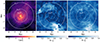 |
Fig. 6. Projected spectroscopic-like temperature (left) and the ratio of the EW sightline velocity (centre) and velocity dispersion (right) over the sound speed in each pixel, which is thus a local Mach number, along the x sightline. The solid, dashed and dotted white circles respectively represent Rvir, R500 and R2500. |
We used both the MW and EW projections for the sightline velocity and velocity dispersion, σlos. In addition, we computed the standard deviation of the sightline velocity, σproj, as already presented in Fig. 5. We present the results in Fig. 7. The left (right) panel presents the values estimated within R500 (Rvir). The Mach number (x-axis) is compared to the velocity dispersion, σ (top), and the non-thermal pressure fraction (bottom). All the values displayed in this figure can be found in Table D.1.
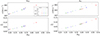 |
Fig. 7. Mach number (x-axis) compared to the velocity dispersion, σ, (top) and the non-thermal pressure fraction (bottom). The left (right) panel presents the quantities computed within R500 (Rvir). Each marker represents a method to compute the velocity dispersion: dots for the 3D, ‘plus’ (square) for the sightline velocity dispersion and cross (diamond) for the standard deviation over the sightline velocity, both from EW (MW) projections. The values derived from the norm of the 3D velocity field are displayed in black. The quantities derived from the x, y, z, and cen components (indeed only x, y, z) or projections are respectively displayed in red, blue, green and pink. |
For both radii, the temperature estimated from the 3D simulation outputs is higher than that calculated from spectroscopic-like projected temperatures (see Table D.1). This leads to a sound speed higher than 1300 (1200) km s−1 within R500 (Rvir), whereas it is below 1200 (1000) km s−1 for the projected counterparts. Nevertheless, this difference only leads to a difference of approximately a few percent in the Mach number estimation for a fixed velocity dispersion of, for example, 250 km s−1. Thus, the velocities are distributed around 0 km s−1 (see also Table D.1), except for the cen projection, which is around 100 km s−1, for both radii, due to matter accretion from the aligned background filament. Whatever the value of the velocity, it is always much lower than the velocity dispersion, which is distributed roughly between 100 and 300 km s−1 (see top panels of Fig. 7) for both radii and thus dominates over the velocity. We clearly see this by the almost linear correlation between σ and M3D. There is also an expected correlation between Pnt/Ptot and M3D on the bottom sub-panels of Fig. 7. For the 3D components and norm, we have a Mach number of about [0.32, 0.35] ([0.4, 0.5]) within R500 (Rvir), leading to a non-thermal pressure fraction of around 6% (9%). For the projected values, on the one hand, in both radii and for both weighting methods, the sightline velocity dispersion of σlos is (as expected) in good agreement with the 1D velocity dispersion of the 3D velocity field, and so are the Mach number and the non-thermal pressure fraction. On the other hand, σproj is much lower (as shown in the top panel of Fig. 5), so the estimated Mach number and non-thermal pressure fraction are also much lower in the 2.5 to 4% range (3 to 6%) within R500 (Rvir). The three exceptions are the x 3D component and the x and cen projections, for which we show significant projection effects due to accretion from filaments; these lead to a very large velocity dispersion, and hence to a non-thermal pressure fraction up to 10% within R500. Within Rvir, only the x component and projection have an overestimated velocity dispersion of about 300 km s−1, leading to a non-thermal pressure fraction of 15%.
The Mach numbers estimated within R500, either from 3D or sightline velocity dispersion, are in rather good agreement with the values estimated by Gatuzz et al. (2022b), though the latter are estimated within a very central region, as we discuss further in Sect. 6. Moreover, the fraction of non-thermal pressure, even for our x component and projection, is in good agreement with most of the values found by Eckert et al. (2019) using the X-COP sample at R500. The exception is A2319, which has a non-thermal pressure fraction higher than 40% at both radii. Similarly to Eckert et al. (2019), our values are slightly below those of Nelson et al. (2014) and The300, but also Gianfagna et al. (2021) and those of Sarkar et al. (2025) obtained with a joint SPT4 and XMM-Newton5 analysis.
5. Velocity structure function
After estimating the non-thermal pressure fraction, which is assumed to result mostly from turbulence, we now use the velocity structure function (VSF) to characterise the structuration of the velocity distribution across scales and thus assess the presence of the turbulent cascade. The n-th order VSF, written δvn(r) hereafter, is the n-th moment of the absolute velocity difference of all data points separated by a distance, r. In the core of this study, we only considered a constant weight (see Fig. B.4 for a density-weighted VSF). The VSF is thus written as
 (5)
(5)
with v being the sightline velocity and N the number of data points separated by a distance, r.
Best-fit values of the velocity structure function slope.
We computed the first- and second-order VSFs. The first order is simply the mean absolute velocity difference and thus informs us of the general gas flow, while the second-order VSF is equal to twice the variance minus the correlation function (see e.g. Schulz-DuBois & Rehberg 1981). The first- and second-order VSFs are respectively presented in Figs. 8 and B.2. For both figures, the VSF was computed from EW and MW maps, which are presented in the left panel for the former and the right panel for the latter. The comparison of the VSF computed from the EW and MW maps for a given projection can be found in Appendix B. The separation between pixels in the maps ranges between 22.5 kpc, which is a pixel width, and 7065 kpc, in the diagonal of the map. The VSFs were thus binned in 100 intervals on a log scale in this range. Given the small number of values in the bins at the shortest and longest separations (see Fig. B.1), we defined the range of validity between 100 and 4000 kpc for this analysis.
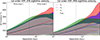 |
Fig. 8. First order velocity structure function (VSF) computed from EW (left) and MW projected maps (right). They are displayed in red for the vx projection, blue for the vy projection, green for the vz projection and pink for the vcen projection. The dispersions are displayed in shaded areas in the same colours. They are presented in the [100, 4000] kpc range, considered as the range of validity of the study (see left panel of Fig. B.1). The range is separated into two fitting ranges: [100, 600] kpc and [600, 1000] kpc, separated by a dashed vertical dotted black line on the plot. The best-fit slope values in each interval are reported in Table 1. |
We observe that, regardless of the order and for both the EW and MW maps, the VSFs seem to have roughly the same slope in the [100, 600] kpc range, but behave very differently in the [600, 4000] kpc range. We named these two intervals ‘Fitting range 1’ and ‘Fitting range 2’, in which we fitted a power-law δvn(r) = Arα. A dotted vertical black line highlights the delimitation. The best-fit values of the slope, α, are reported in Table 1. It is worth noting that the uncertainties on the best-fit value of the slope are of the order of 10−4 and are thus not reported in the table. It confirms that the VSFs have very similar slopes in the first fitting range, although with a bit more dispersion for the second-order VSF of the MW projections.
In the [600, 4000] kpc range, the differences in slope reflect the contribution of the filaments connected to Virgo. As a matter of fact, the bimodality observed in the vx projection induces large velocity differences at large separations, leading to the steepest VSF slope among the projections. We notice that the slope is steeper for the MW method because this method smooths the projection compared to the EW method, which has the combined effect of lowering the contribution of density peaks while leveraging the contribution of underdense regions. It is particularly visible at the bottom of the projection (left panels of Fig. 1), where the EW projection has a very negative velocity region, but the rest is closer to zero. In contrast, the MW projection has a velocity distribution of around −400 km s−1 in the same bottom part. It is also visible on the PDFs (top left panel of Fig. 3). The EW projection has pixels with lower velocities than the MW projection, but has much less weight in the left tail. In contrast, the vcen projection has the lowest slope. The VSF almost flattens in this range, which is expected because it is dominated by the gas flow from the background filament; this can be considered as coherent and thus has low-velocity gradients. The MW method has a lower slope for that projection than its EW counterpart, given that it just smooths the velocity field, which is not as contrasted as the vx projection. Finally, the vy and vz projections have intermediate VSF slopes, although they tend to flatten beyond a 1 Mpc separation, which could mean that there is no turbulent cascade on these scales. As shown by the visual inspection of the projections in Fig. 1 and the analysis of their PDFs in Fig. 3, these two projections are the least impacted by the filaments connected to Virgo. They would thus be the most representative of an ideal, relaxed, and isolated cluster.
Given the similarity of the slope in all the projections in the first fitting range, we could consider it the inertial range where the turbulent cascade occurs. In that scenario, the injection scale, i.e. the size of the largest vortices before collapsing into smaller ones, would be in the [600, 800] kpc range. This typical scale is roughly the diameter of the AGN shockfront observed in Lebeau et al. (2024a), which could contribute to generating vortices and, thus, turbulence in Virgo’s core. On the other hand, we cannot observe the dissipation scale at small separations, which we might observe on much better resolved projected maps, but it is beyond the scope of this study. The second fitting range highlights the level of contribution of local large-scale structures along some sightlines. In terms of slope, the Kolmogorov theory (Kolmogorov 1941) predicts δvn(r)∝rn/3 in the inertial range for the n-th order VSF, whereas the computed VSFs are much steeper and seem closer to δvn(r)∝r(n + 1)/3. It might mostly be due to projection effects steepening the VSF, as observed by Mohapatra et al. (2022) or Fournier et al. (2025), for example, since we showed in Lebeau et al. (2025) that the 3D velocity power spectrum (which is the Fourier transform of the second-order VSF) in the core of the Virgo replica is in excellent agreement with the Kolmogorov prediction. This finding is in agreement with Vazza & Brunetti (2026), which showed that the 3D second-order VSF of their Coma-like simulated cluster is also in good agreement with Kolmogorov-like turbulence on a rather large range of scales.
6. Discussion
Throughout this work, we used both the EW and MW methods to project and quantify the velocity field of Virgo’s ICM through different tracers. We explain the motivations for the use of these weighting methods and summarise the different results yielded by each of them.
On the one hand, the MW method is physically motivated when averaging over intensive physical quantities such as the pressure, temperature, or velocity, given that the cells or particles extracted from cosmological simulations have different masses. For instance, this method is widely used in analyses of direct outputs of simulations to compute radial profiles of several properties of galaxy clusters. We used it to project the pressure along multiple sightlines in Lebeau et al. (2024a); we thus logically tested this method on the velocity field in this work. On the other hand, the EW method is used to mimic observed quantities without fully reproducing them since the weight is the squared electron density (similarly to the X-ray’s surface brightness); it is thus used in mock X-ray observations such as Biffi et al. (2012) or Roncarelli et al. (2018), including the sightline velocity and velocity dispersion as in this study. It was also shown by Mazzotta et al. (2004) and Rasia et al. (2005) that the spectroscopic-like weighting method is a better approximation than the EW one to reproduce the observed spectroscopic temperature. We thus followed this approach for the temperature. For the sightline velocity and velocity dispersion, there is not, to our knowledge, a thorough comparison between the MW and EW methods in the literature.
For the sightline velocity, we observed that the EW projections are more contrasted than their MW counterpart (see Fig. 1), thus leading to a larger standard deviation. However, in both cases, the standard deviation is much lower than its simulated counterpart, as shown in the top panel of Fig. 5. In addition, the mean velocity extracted within R2500, R500, or Rvir on these sightline velocities is centred on zero over the 100 random projections for both methods. The VSFs computed from the EW projections have a higher amplitude and slightly higher slope than the MW ones in the [100, 600] kpc range, as shown in Table 1 and compared in Fig. B.3, but the general trend remains the same. However, beyond 600 kpc, in the case of large projection effects induced by filaments such as in the x projection, the smoother MW projection leads to a steeper VSF because the number of pairs with important velocity difference is larger than its more peaked EW counterpart.
For the sightline velocity dispersion (see Fig. A.1), the EW projections are also more peaked, but the mean velocity dispersion is on average smaller than for MW projections (see bottom panel of Fig. 5). It is inverted compared to the standard deviation of sightline velocity. This is due to the fact that EW sightline velocity is used to compute the EW sightline velocity dispersion (see second member of Eq. 2). Since it is more contrasted, it yields a higher squared sightline velocity than its MW equivalent, leading to smaller sightline velocity dispersion than with the MW method. We observe that the MW σlos/σsim ratio is the closest to one at each radius, leading to the most accurate non-thermal pressure fraction estimation when considering the MW, direct simulation outputs as the ground-truth. Thus, in a simulation-oriented approach, like this work, the MW projections should be preferred to the EW ones to study the velocity field along sightlines, particularly when studying non-thermal pressure. However, it does not show that the MW method should be used instead of the EW method for mock observations.
The VSF is increasingly being used to quantify turbulence in the ICM. On the simulation side, for example Mohapatra et al. (2022) and Fournier et al. (2025), the VSF was computed in the core of clusters, accounting for multiple phases of the gas, magnetic fields, and sub-grid turbulence driving method for the former. They find that the different phases of the gas seem to have uncorrelated VSFs; we did not explore this question in our work since we focused on the hot phase of the gas. In addition, by comparing 3D VSFs to mock observations, Fournier et al. (2025) also found that projection effects can reduce the amplitude and thus induce a slightly steeper VSF slope. In addition to effects induced by physics processes in the ICM, projection effects could partially contribute to explaining the steep VSF slope we observed in our work. This could be tested by comparing 3D VSFs to VSFs computed from mock observations, which will be estimated in a future project. Finally, Li et al. (2025) compared the VSF of [OII] emission lines emitted by warm gas of central galaxies of four clusters to that of cold molecular gas probed by ALMA CO emission and to Chandra X-ray surface brightness fluctuations. They find a relatively good agreement between the VSF of the three phases, particularly between the cold and warm phases, although they mention that their conclusions have to be taken with caution since systematics and projection effects may bias the results. In this work, we purposely focused on the hot phase of the gas, but the resolution of our simulation, down to 0.3 kpc in the most resolved regions, is sufficient to conduct a study focusing on Virgo’s core and explore its different phases to compare to the aforementioned studies, which we might do in the future.
Our work is complementary to previous studies of turbulence in Virgo since it focuses on the hot phase of the ICM at larger scales and up to Rvir. For instance, Li et al. (2020) computed the VSF of Hα filaments, i.e. the cold phase of the ICM, using optical MUSE data, and Zhuravleva et al. (2018) analysed X-ray surface brightness fluctuations with Chandra. Both these studies focused on the core of Virgo; we thus cannot directly compare their works to ours.
Recently, Gatuzz et al. (2023a) computed the VSF of the ICM of the Virgo cluster from XMM-Newton observations. However, in their study, they computed the VSF at much smaller scales because the observation was centred on the core of Virgo to obtain a sufficiently high signal-to-noise ratio. They computed the VSF in the [3, 180] kpc range, observing a flattening on an ∼15 kpc scale, which they consider as a possible driving scale, and a slope of roughly 2/3 at smaller separations. Given that we computed the VSF on scales larger than 22 kpc and considered the range of validity to be [100, 4000] kpc, we can hardly compare our results to theirs. Still, it might be worth noting that we observe a similar 2/3 slope in the [100, 600] kpc range and that, given that we observe a potential injection scale at about 600 kpc, we would rather expect a dissipation scale below 20 kpc than another injection scale of the hot phase of the ICM.
In addition, Gatuzz et al. (2023a) studied the statistical properties of the velocity field in the core of Virgo. Due to the limited spectral resolution of the EPIC-pn instrument, they were not able to access the sightline velocity dispersion; this will be possible with XRISM and NewAthena. Nonetheless, they estimated the standard deviation of the observed sightline velocities by fitting their distributions to a Gaussian law. For Virgo, they found a standard deviation of 344 ± 18 km s−1, which is much higher than any of our results, particularly the standard deviation of the vcen projection that is 157.8 km s−1 at maximum. Even the standard deviation of the x component of the 3D velocity field within Rvir, which is the highest value that we showed to be contaminated by accretion from filaments, has a lower standard deviation of 325.6 km s−1. Figure 9 compares the value of their best-fit standard deviation to the distribution of the standard deviation for the 100 randomly oriented projections of sightline velocity within R2500 ≈ 500 kpc. It shows that their value is incompatible with our results, even more so given that their estimation comes from a very central region of the cluster, i.e. less than (100 kpc)2, and that we observe a decreasing standard deviation when decreasing the radius in which it is estimated in our simulation.
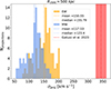 |
Fig. 9. Comparison between σproj of the hundred randomly oriented projections within R2500, as already presented in top left panel of Fig. 5 this time not divided by σsim, and the best-fit value of the standard deviation found in Gatuzz et al. (2023a) displayed as a red dashed vertical line within a shaded area representing the uncertainty. |
Before concluding, we summarise the key properties of the Virgo replica simulation impacting the results and the tests conducted on modelling aspects, in particular weighting methods. We also discuss the limitations and possible improvements of this study. First, on the simulation itself, this Virgo replica simulation has the great advantage of being a constrained simulation, thus reproducing the Virgo cluster with great fidelity; this includes its local environment, which we found to play a major role in the gas dynamics and to induce important projection effects. Moreover, this simulation contains a refined AGN feedback model in addition to standard sub-grid models, thus properly accounting for non-gravitational processes, but without implementing a sub-grid model of turbulence (as in e.g. Iapichino et al. 2017). Finally, this Virgo replica’s finest AMR cell resolution is 0.35 kpc, thus permitting to develop turbulence down to scales that cannot currently be reached by X-ray observatories. To get closer to scales reachable by current facilities, we produced projections with a resolution of 22.5 kpc (corresponding to a coarser level of refinement of the AMR grid), thus using physical quantities averaged on those scales. This choice indeed reduces the spatial resolution and prevents the study of small-scale features, but, on the other hand, it uses reliable averaged quantities and allows much quicker computation; in particular for the VSF for which we showed (see right panel of Fig. B.1) that a twice as resolved projection yields a very similar result. Then, we discussed the impact of the weighting schemes for the projections, showing that MW projections give results closer to our ground-truth 3D velocity field. We also tested the impact of the weighting scheme of the VSF, using either a constant- or density-weighted scheme (see Fig. B.4), showing similar results except for the Cen projection that is strongly impacted by projection effects. We also found that the 2D VSF does not follow the Kolmogorov prediction, which is certainly due to projection effects and needs to be investigated further. However, two limitations of our study are that we did not estimate the uncertainties on the measured velocity dispersion, as tackled in, for example, Roncarelli et al. (2018) and in the Clerc et al. (2019), Cucchetti et al. (2019), Beaumont et al. (2024), Molin et al. (2025) series of papers, and we did not account for all the instrumental effects. We plan to extend this study in the near future by producing mock observations of XRISM Resolve or New-Athena X-IFU, in which the instrumental effects and uncertainties will be accounted for.
7. Conclusion
In this work, we studied the velocity field in the ICM of the Virgo cluster’s simulated replica. We first characterised the statistical properties of the velocity field by computing the PDF and the statistical moments of its components from both 3D simulation outputs and projected velocity maps, first in four sightlines and then among 100 random projections. Using the velocity dispersion, we then estimated the non-thermal pressure fraction through an effective turbulent Mach number. Finally, we computed the VSF of the projected velocity maps. We also discussed the results found using either MW or EW projections and the difference in velocity-dispersion estimation between the sightline velocity dispersion and the standard deviation over the sightline velocity in light of other studies.
The analysis of the PDFs and the statistical moments shows that the 3D velocity field is not isotropic, particularly in the outskirts, where cosmic gas is accreted at high velocities. It is also not homogeneous as the PDFs tighten up, so the standard deviation reduces when reducing the radius of the sphere from which the gas cells are extracted. Choosing to study the velocity field within R500 seems to be a good compromise as it is a large enough radius to be statistically representative of the global velocity field, and thus it is neither biased by homogeneities nor too contaminated by the contribution of gas accreted in the outskirts. The projected velocity fields are subject to important projection effects along the x and cen sightlines, given that the latter are quite aligned with filaments connected to Virgo and matter funnelling into it. Overall, the 2D PDFs have smaller dispersions compared to their 3D counterpart, and the MW method shrinks the distributions even more as it smooths the distribution, whereas the EW method highlights the densest regions, leading to more contrasted projections. Generalising over a hundred random projections, we confirmed that the standard deviation of sightline velocity is much lower than its 3D counterpart, but the sightline velocity dispersions, particularly the MW ones, are, on the contrary, in good agreement.
We then estimated the non-thermal pressure fraction using the velocity dispersion included in an effective turbulent Mach number. We find a non-thermal pressure fraction of about 6% within R500 and 9% within Rvir from direct 3D simulation outputs. The non-thermal pressure fractions estimated using MW sightline velocity dispersion are in good agreement, whereas all the other methods yield a lower value. We also notice the impact of important projection effects for the x component of the 3D velocity field and its associated projection, leading to an overestimation of this fraction by several percent.
The first and second-order VSFs of the projected velocity maps have similar slopes below 600 kpc for both EW and MW maps. This range could be considered as the inertial range of the turbulent cascade, so the injection scale, and thus the diameter of the largest eddy, which could be related to the size of the AGN feedback shockfront. Beyond this scale, the VSF shows the contribution of the local large-scale structure, as it increases significantly with separation for the vx projected map but more or less flattens for the others. Moreover, we found much steeper slopes than Kolmogorov’s predictions, at all scales, indicating that the turbulence in the ICM of this cluster is much more complex than the ideal case.
To conclude, the case study of the velocity field in the ICM of the Virgo replica shows how complex its gas dynamics is. It is highly turbulent, and both filaments in the outskirts and the AGN in the core bring energy to the medium and induce a consequential amount of non-thermal pressure. We postpone a systematic study of the impact of this on the reconstruction of the hydrostatic mass to a forthcoming work. Moreover, constraining the properties of the ICM from observations with XRISM and NewAthena will improve our understanding of velocities within the ICM, but there is still a lot to explore on the simulation, theory, and mock observation side to be able to properly analyse the upcoming data.
Acknowledgments
The authors acknowledge the Gauss Centre for Supercomputing e.V. (https://www.gauss-centre.eu) for providing computing time on the GCS Supercomputers SuperMUC at LRZ Munich. This work was supported by the grant agreements ANR-21-CE31-0019/490702358 from the French Agence Nationale de la Recherche/DFG for the LOCALIZATION project. This work has been supported as part of France 2030 program ANR-11-IDEX-0003. SE acknowledges the financial contribution from the contracts Prin-MUR 2022 supported by Next Generation EU (n.20227RNLY3 The concordance cosmological model: stress-tests with galaxy clusters), ASI-INAF Athena 2019-27-HH.0, “Attività di Studio per la comunità scientifica di Astrofisica delle Alte Energie e Fisica Astroparticellare” (Accordo Attuativo ASI-INAF n. 2017-14-H.0), from the European Union’s Horizon 2020 Programme under the AHEAD2020 project (grant agreement n. 871158), and the support by the Jean D’Alembert fellowship program. The authors thank the IAS Cosmology team members and Nicholas Battaglia for the discussions and comments. The authors thank Florent Renaud for sharing the rdramses RAMSES data reduction code.
References
- Adam, R., Eynard-Machet, T., Bartalucci, I., et al. 2025, A&A, 694, A182 [NASA ADS] [CrossRef] [EDP Sciences] [Google Scholar]
- Angelinelli, M., Vazza, F., Giocoli, C., et al. 2020, MNRAS, 495, 864 [NASA ADS] [CrossRef] [Google Scholar]
- Aymerich, G., Douspis, M., Pratt, G. W., et al. 2024, A&A, 690, A238 [NASA ADS] [CrossRef] [EDP Sciences] [Google Scholar]
- Ayromlou, M., Nelson, D., Pillepich, A., et al. 2024, A&A, 690, A20 [NASA ADS] [CrossRef] [EDP Sciences] [Google Scholar]
- Beaumont, S., Molin, A., Clerc, N., et al. 2024, A&A, 686, A41 [NASA ADS] [CrossRef] [EDP Sciences] [Google Scholar]
- Biffi, V., Dolag, K., Böhringer, H., & Lemson, G. 2012, MNRAS, 420, 3545 [NASA ADS] [Google Scholar]
- Biffi, V., Borgani, S., Murante, G., et al. 2016, ApJ, 827, 112 [NASA ADS] [CrossRef] [Google Scholar]
- Bourne, M. A., & Sijacki, D. 2017, MNRAS, 472, 4707 [NASA ADS] [CrossRef] [Google Scholar]
- Chira, R.-A., Ibáñez-Mejía, J. C., Mac Low, M.-M., & Henning, T. 2019, A&A, 630, A97 [NASA ADS] [CrossRef] [EDP Sciences] [Google Scholar]
- Churazov, E., Vikhlinin, A., Zhuravleva, I., et al. 2012, MNRAS, 421, 1123 [NASA ADS] [CrossRef] [Google Scholar]
- Clerc, N., Cucchetti, E., Pointecouteau, E., & Peille, P. 2019, A&A, 629, A143 [NASA ADS] [CrossRef] [EDP Sciences] [Google Scholar]
- Cruise, M., Guainazzi, M., Aird, J., et al. 2025, Nat. Astron., 9, 36 [Google Scholar]
- Cucchetti, E., Clerc, N., Pointecouteau, E., Peille, P., & Pajot, F. 2019, A&A, 629, A144 [NASA ADS] [CrossRef] [EDP Sciences] [Google Scholar]
- Dolag, K., Sorce, J. G., Pilipenko, S., et al. 2023, A&A, 677, A169 [NASA ADS] [CrossRef] [EDP Sciences] [Google Scholar]
- Doumler, T., Hoffman, Y., Courtois, H., & Gottlöber, S. 2013, MNRAS, 430, 888 [NASA ADS] [CrossRef] [Google Scholar]
- Dubois, Y., Pichon, C., Welker, C., et al. 2014, MNRAS, 444, 1453 [Google Scholar]
- Dubois, Y., Peirani, S., Pichon, C., et al. 2016, MNRAS, 463, 3948 [Google Scholar]
- Dubois, Y., Beckmann, R., Bournaud, F., et al. 2021, A&A, 651, A109 [NASA ADS] [CrossRef] [EDP Sciences] [Google Scholar]
- Dupourqué, S., Clerc, N., Pointecouteau, E., et al. 2023, A&A, 673, A91 [NASA ADS] [CrossRef] [EDP Sciences] [Google Scholar]
- Dupourqué, S., Clerc, N., Pointecouteau, E., et al. 2024, A&A, 687, A58 [NASA ADS] [CrossRef] [EDP Sciences] [Google Scholar]
- Eckert, D., Ghirardini, V., Ettori, S., et al. 2019, A&A, 621, A40 [NASA ADS] [CrossRef] [EDP Sciences] [Google Scholar]
- Ettori, S., Donnarumma, A., Pointecouteau, E., et al. 2013, Space Sci. Rev., 177, 119 [Google Scholar]
- Fournier, M., Grete, P., Brüggen, M., et al. 2025, A&A, 698, A121 [NASA ADS] [CrossRef] [EDP Sciences] [Google Scholar]
- Gaspari, M., & Churazov, E. 2013, A&A, 559, A78 [NASA ADS] [CrossRef] [EDP Sciences] [Google Scholar]
- Gatuzz, E., Sanders, J. S., Canning, R., et al. 2022a, MNRAS, 513, 1932 [NASA ADS] [CrossRef] [Google Scholar]
- Gatuzz, E., Sanders, J. S., Dennerl, K., et al. 2022b, MNRAS, 511, 4511 [NASA ADS] [CrossRef] [Google Scholar]
- Gatuzz, E., Mohapatra, R., Federrath, C., et al. 2023a, MNRAS, 524, 2945 [NASA ADS] [CrossRef] [Google Scholar]
- Gatuzz, E., Sanders, J. S., Dennerl, K., et al. 2023b, MNRAS, 522, 2325 [NASA ADS] [CrossRef] [Google Scholar]
- Gatuzz, E., Sanders, J., Liu, A., et al. 2024, A&A, 692, A108 [NASA ADS] [CrossRef] [EDP Sciences] [Google Scholar]
- Gianfagna, G., De Petris, M., Yepes, G., et al. 2021, MNRAS, 502, 5115 [NASA ADS] [CrossRef] [Google Scholar]
- Gouin, C., Gallo, S., & Aghanim, N. 2022, A&A, 664, A198 [NASA ADS] [CrossRef] [EDP Sciences] [Google Scholar]
- Groth, F., Valentini, M., Steinwandel, U. P., Vallés-Pérez, D., & Dolag, K. 2025, A&A, 693, A263 [NASA ADS] [CrossRef] [EDP Sciences] [Google Scholar]
- Heinrich, A., Zhuravleva, I., Zhang, C., et al. 2024, MNRAS, 528, 7274 [CrossRef] [Google Scholar]
- Hernández-Martínez, E., Dolag, K., Seidel, B., et al. 2024, A&A, 687, A253 [NASA ADS] [CrossRef] [EDP Sciences] [Google Scholar]
- Hernández-Martínez, E., Dolag, K., Steinwandel, U. P., et al. 2026, A&A, in press, https://doi.org/10.1051/0004-6361/202556542 [Google Scholar]
- Hitomi Collaboration 2016, Nature, 535, 117 [CrossRef] [Google Scholar]
- Hitomi Collaboration 2018, PASJ, 70, 9 [NASA ADS] [CrossRef] [Google Scholar]
- Hoffman, G., Olson, D., & Salpeter, E. 1980, ApJ, 242, 861 [NASA ADS] [CrossRef] [Google Scholar]
- Iapichino, L., Schmidt, W., Niemeyer, J., & Merklein, J. 2011, MNRAS, 414, 2297 [CrossRef] [Google Scholar]
- Iapichino, L., Federrath, C., & Klessen, R. S. 2017, MNRAS, 469, 3641 [NASA ADS] [CrossRef] [Google Scholar]
- Khatri, R., & Gaspari, M. 2016, MNRAS, 463, 655 [Google Scholar]
- Kolmogorov, A. N. 1941, Dokl. Akad. Nauk SSSR, 30, 301 [NASA ADS] [Google Scholar]
- Kravtsov, A. V., & Borgani, S. 2012, A&ARv, 50, 353 [Google Scholar]
- Lebeau, T. 2025, Ph.D. Thesis, Université Paris-Saclay [Google Scholar]
- Lebeau, T., Sorce, J. G., Aghanim, N., Hernández-Martínez, E., & Dolag, K. 2024a, A&A, 682, A157 [NASA ADS] [CrossRef] [EDP Sciences] [Google Scholar]
- Lebeau, T., Ettori, S., Aghanim, N., & Sorce, J. G. 2024b, A&A, 689, A19 [NASA ADS] [CrossRef] [EDP Sciences] [Google Scholar]
- Lebeau, T., Zaroubi, S., Aghanim, N., Sorce, J. G., & Langer, M. 2025, A&A, 704, A14 [NASA ADS] [CrossRef] [EDP Sciences] [Google Scholar]
- Li, H., & Gnedin, O. Y. 2014, ApJ, 796, 10 [Google Scholar]
- Li, Y., Gendron-Marsolais, M.-L., Zhuravleva, I., et al. 2020, ApJ, 889, L1 [NASA ADS] [CrossRef] [Google Scholar]
- Li, M., McNamara, B. R., Coil, A. L., et al. 2025, ApJ, 984, 22 [Google Scholar]
- Lovisari, L., Ettori, S., Rasia, E., et al. 2024, A&A, 682, A45 [NASA ADS] [CrossRef] [EDP Sciences] [Google Scholar]
- Martizzi, D., Vogelsberger, M., Artale, M. C., et al. 2019, MNRAS, 486, 3766 [Google Scholar]
- Mazzotta, P., Rasia, E., Moscardini, L., & Tormen, G. 2004, MNRAS, 354, 10 [NASA ADS] [CrossRef] [Google Scholar]
- Mohapatra, R., Federrath, C., & Sharma, P. 2020, MNRAS, 493, 5838 [NASA ADS] [CrossRef] [Google Scholar]
- Mohapatra, R., Jetti, M., Sharma, P., & Federrath, C. 2022, MNRAS, 510, 3778 [NASA ADS] [CrossRef] [Google Scholar]
- Molin, A., Dupourqué, S., Clerc, N., et al. 2025, A&A, 702, A215 [NASA ADS] [CrossRef] [EDP Sciences] [Google Scholar]
- Moran, C. C., Teyssier, R., & Lake, G. 2014, MNRAS, 442, 2826 [NASA ADS] [CrossRef] [Google Scholar]
- Nagai, D., Kravtsov, A. V., & Vikhlinin, A. 2007, ApJ, 668, 1 [Google Scholar]
- Nagai, D., Lau, E. T., Avestruz, C., Nelson, K., & Rudd, D. H. 2013, ApJ, 777, 137 [NASA ADS] [CrossRef] [Google Scholar]
- Nelson, K., Lau, E. T., & Nagai, D. 2014, ApJ, 792, 25 [NASA ADS] [CrossRef] [Google Scholar]
- Norman, M. L., & Bryan, G. L. 1999, The Radio Galaxy Messier 87: Proceedings of a Workshop Held at Ringberg Castle, Tegernsee, Germany, 15–19 September 1997, Springer, 106 [Google Scholar]
- Planck Collaboration XVI. 2014, A&A, 571, A16 [NASA ADS] [CrossRef] [EDP Sciences] [Google Scholar]
- Porter, D. H., Jones, T., & Ryu, D. 2015, ApJ, 810, 93 [NASA ADS] [CrossRef] [Google Scholar]
- Pratt, G., Arnaud, M., Biviano, A., et al. 2019, Space Sci. Rev., 215, 1 [CrossRef] [Google Scholar]
- Rasia, E., Tormen, G., & Moscardini, L. 2004, MNRAS, 351, 237 [NASA ADS] [CrossRef] [Google Scholar]
- Rasia, E., Mazzotta, P., Borgani, S., et al. 2005, ApJ, 618, L1 [NASA ADS] [CrossRef] [Google Scholar]
- Renaud, F., Bournaud, F., Emsellem, E., et al. 2013, MNRAS, 436, 1836 [NASA ADS] [CrossRef] [Google Scholar]
- Romero, C. E., Gaspari, M., Schellenberger, G., et al. 2023, ApJ, 951, 41 [NASA ADS] [CrossRef] [Google Scholar]
- Romero, C. E., Gaspari, M., Schellenberger, G., et al. 2024, ApJ, 970, 73 [NASA ADS] [CrossRef] [Google Scholar]
- Roncarelli, M., Gaspari, M., Ettori, S., et al. 2018, A&A, 618, A39 [NASA ADS] [CrossRef] [EDP Sciences] [Google Scholar]
- Salvati, L., Douspis, M., & Aghanim, N. 2018, A&A, 614, A13 [NASA ADS] [CrossRef] [EDP Sciences] [Google Scholar]
- Sarazin, C. L. 1986, Rev. Mod. Phys., 58, 1 [Google Scholar]
- Sarkar, A., McDonald, M., Bleem, L., et al. 2025, ApJ, 984, L63 [Google Scholar]
- Sawala, T., McAlpine, S., Jasche, J., et al. 2022, MNRAS, 509, 1432 [Google Scholar]
- Schuecker, P., Finoguenov, A., Miniati, F., Böhringer, H., & Briel, U. 2004, A&A, 426, 387 [NASA ADS] [CrossRef] [EDP Sciences] [Google Scholar]
- Schulz-DuBois, E., & Rehberg, I. 1981, Appl. Phys. A, 24, 323 [Google Scholar]
- Shi, X., Nagai, D., & Lau, E. T. 2018, MNRAS, 481, 1075 [NASA ADS] [CrossRef] [Google Scholar]
- Simionescu, A., ZuHone, J., Zhuravleva, I., et al. 2019, Space Sci. Rev., 215, 24 [NASA ADS] [CrossRef] [Google Scholar]
- Simonte, M., Vazza, F., Brighenti, F., et al. 2022, A&A, 658, A149 [NASA ADS] [CrossRef] [EDP Sciences] [Google Scholar]
- Sorce, J. G., Gottlöber, S., Yepes, G., et al. 2016, MNRAS, 455, 2078 [NASA ADS] [CrossRef] [Google Scholar]
- Sorce, J. G., Blaizot, J., & Dubois, Y. 2019, MNRAS, 486, 3951 [NASA ADS] [CrossRef] [Google Scholar]
- Sorce, J. G., Dubois, Y., Blaizot, J., et al. 2021, MNRAS, 504, 2998 [NASA ADS] [CrossRef] [Google Scholar]
- Sotira, S., Vazza, F., & Brighenti, F. 2025, A&A, 697, A138 [NASA ADS] [CrossRef] [EDP Sciences] [Google Scholar]
- Sunyaev, R., & Zeldovich, Y. B. 1972, Comments Astrophys. Space Phys., 4, 173 [Google Scholar]
- Teyssier, R. 2002, A&A, 385, 337 [CrossRef] [EDP Sciences] [Google Scholar]
- Tully, R. B., Courtois, H. M., Dolphin, A. E., et al. 2013, AJ, 146, 86 [NASA ADS] [CrossRef] [Google Scholar]
- Tweed, D., Devriendt, J., Blaizot, J., Colombi, S., & Slyz, A. 2009, A&A, 506, 647 [NASA ADS] [CrossRef] [EDP Sciences] [Google Scholar]
- Vallés-Pérez, D., Planelles, S., & Quilis, V. 2021, MNRAS, 504, 510 [CrossRef] [Google Scholar]
- Vazza, F., & Brunetti, G. 2026, A&A, 705, A129 [NASA ADS] [CrossRef] [EDP Sciences] [Google Scholar]
- Vazza, F., Brüggen, M., & Gheller, C. 2013, MNRAS, 428, 2366 [NASA ADS] [CrossRef] [Google Scholar]
- Vazza, F., Jones, T. W., Brüggen, M., et al. 2017, MNRAS, 464, 210 [Google Scholar]
- Wang, H., Mo, H. J., Yang, X., Jing, Y. P., & Lin, W. P. 2014, ApJ, 794, 94 [NASA ADS] [CrossRef] [Google Scholar]
- Wang, C., Ruszkowski, M., Pfrommer, C., Oh, S. P., & Yang, H. K. 2021, MNRAS, 504, 898 [NASA ADS] [CrossRef] [Google Scholar]
- Wang, C., Oh, S. P., & Ruszkowski, M. 2023, MNRAS, 519, 4408 [Google Scholar]
- XRISM Collaboration (Audard, M., et al.) 2025a, ApJ, 982, L5 [Google Scholar]
- XRISM Collaboration (Audard, M., et al.) 2025b, PASJ, 77, S242 [Google Scholar]
- XRISM Collaboration (Audard, M., et al.) 2025c, ApJ, 985, L20 [Google Scholar]
- XRISM Collaboration (Audard, M., et al.) 2025d, ApJ, 993, L11 [Google Scholar]
- XRISM Science Team 2020, arXiv e-prints [arXiv:2003.04962] [Google Scholar]
- Zhu, L., Long, R., Mao, S., et al. 2014, ApJ, 792, 59 [CrossRef] [Google Scholar]
- Zhuravleva, I., Churazov, E., Kravtsov, A., & Sunyaev, R. 2012, MNRAS, 422, 2712 [NASA ADS] [CrossRef] [Google Scholar]
- Zhuravleva, I., Churazov, E. M., Schekochihin, A. A., et al. 2014, ApJ, 788, L13 [Google Scholar]
- Zhuravleva, I., Allen, S. W., Mantz, A., & Werner, N. 2018, ApJ, 865, 53 [CrossRef] [Google Scholar]
- ZuHone, J. 2011, ApJ, 728, 54 [NASA ADS] [CrossRef] [Google Scholar]
https://github.com/florentrenaud/rdramses, first used in Renaud et al. (2013).
Appendix A: Sightline velocity dispersion projections
In Fig. A.1, we show the sightline velocity dispersion alike the sightline velocity presented in Fig. 1. The projections seem more contrasted with the emission weighting (top), similarly to the sightline velocity. Moreover, the peaks of velocity dispersion are associated with peaks of sightline velocity, both positive and negative, which shows that although the mean integrated velocity is dominated by the extreme values, there are also smaller velocities contributing along the sightline, which is expected.
 |
Fig. A.1. Projected velocity dispersion integrated along the vx, vy, vz and vcen sightlines from left to right. The top (bottom) row presents the EW (MW) projections. The solid, dashed and dotted black circles respectively represent Rvir, R500 and R2500. |
Appendix B: Complementary VSF figures
In this section of the Appendix, we show figures completing Sect. 5. First, on Fig. B.1, we show the full range of scales of the VSF on the left panel, and we compare the VSF computed on maps with the resolution used for this study (2222) and twice this resolution (4442) on the right panel, showing an excellent agreement. Second, in Fig. B.2, we show the second-order VSF that is discussed in the core of the article. In Fig. B.3, we compare the first (top) and second (bottom) VSFs computed on EW (colored) and MW (grey) projections. Finally, in Fig. B.4, we compare two weighting methods to compute the VSF, either constant- or density-weighted (used in e.g. Ayromlou et al. 2024). The n-th order density-weighted VSF writes as follows (see e.g. Chira et al. 2019):
 (B.1)
(B.1)
with ρ the gas density. In our case, we used the projected electron column density as already used in (Lebeau et al. 2024a). We can see that the density-weighted VSF, whose 2nd order is displayed in black in Fig. B.4, shows a very similar amplitude, though slightly higher, and slope compared to the constant-weighted VSF, which is displayed in colours for the EW case (top) and in grey for the MW case (bottom). The only exception is the Cen projection (right panels) for which the amplitude is much higher and the slope steeper for r< 600 kpc, though still in the same range of amplitude and slope as the other projections’ VSF. This result can be explained by the fact that (i) the sightline velocity is close to zero or even negative in the bottom part of the core (see right panels of Fig. 1), the pairs including these pixels have thus an higher absolute velocity difference and (ii) that because the core of the ICM is the densest region, the pairs including pixels in this region core have much more weight than other pairs, explaining why the average velocity difference rises for r< 600 kpc. It shows that, in the case of a very strong projection effect due to a filament, its impact can be partly mitigated by computing the density-weighted VSF instead of the constant-weighted since it gives more weight to the velocity in the ICM than in the outskirts.
 |
Fig. B.1. Left: Definition of the range of validity of the VSF, [0.1,4] Mpc, given the number of values per bin shown on the bottom sub-panel. Right: Comparison of the VSF computed from 2222 and 4442 pixel maps. The relative difference is shown on the bottom sub-panel. |
 |
Fig. B.2. Second order velocity structure function (VSF) computed from EW (left) and MW projected maps (right). They are displayed in red for the vx projection, blue for the vy projection, green for the vz projection and pink for the vcen projection. The dispersions are displayed in shaded areas in the same colours. They are presented in the [100,4000] kpc range, which is the range of validity of the study given the low number of pairs in bins with smaller and larger separations (see left panel of Fig. B.1). The range is separated into two fitting ranges: [100,600] kpc and [600,1000] kpc; the delimitation between the two intervals is highlighted by a dashed vertical dotted black line. The best-fit slope values in each interval are reported in Table 1. |
 |
Fig. B.3. Comparison of the EW and MW (grey) VSFs at the first (top) and second order (bottom). |
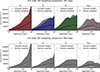 |
Fig. B.4. Comparison of the weighting methods used to compute the VSF. The second-order VSF is presented for EW (top) and MW (bottom). We compare the constant-weighted VSF, represented by coloured lines on the top panel and grey lines on the bottom panel, to the density-weighted VSF, displayed in black. |
Appendix C: Velocity fields statistics
We provide the values of the statistical properties of the PDFs presented in Sect. 3.
Statistical properties of the velocity fields.
Appendix D: Non-thermal pressure and Mach number values
We provide the values of the quantities calculated in Sect. 4 within R500 in the top sub-panel and within Rvir in the bottom sub-panel.
Values of the temperature, sound speed, velocity, velocity dispersion, Mach number and non-thermal pressure fraction.
All Tables
Values of the temperature, sound speed, velocity, velocity dispersion, Mach number and non-thermal pressure fraction.
All Figures
|
Fig. 1. Projections of the velocity integrated along the vx, vy, vz and vcen sightlines from left to right. The top (bottom) row presents the EW (MW) maps. The solid, dashed and dotted black circles respectively represent Rvir, R500 and R2500. The colour bar goes from −600 km s−1 (blue), meaning an average gas flow coming from the foreground of Virgo and going away from the observer, to 600 km s−1 (red), meaning, inversely, an average gas flow coming from the background of Virgo and coming toward the observer. |
| In the text | |
|
Fig. 2. PDFs of the three components of the velocity field within Rvir = 2147 kpc, R500 = 1087 kpc, and R2500 = 515 kpc. The first three rows display the PDFs computed within spheres of decreasing radius from top to bottom. The first three columns display the PDF of each component of the velocity field, vx, from red to yellow, vy in shades of blue, and vz in shades of green, from left to right. The right column overlays the PDFs of the three velocity-field components in a given sphere, and the bottom row overlays the PDFs of a given velocity-field component inside the different spheres. Fitted Gaussian envelopes are displayed as solid black curves. The statistical moments of the PDFs and the best-fit values of the Gaussian fit can be found in Table C.1. |
| In the text | |
|
Fig. 3. 2D PDFs of EW and MW maps computed within circles of the radii Rvir, R500, and R2500 from top to bottom, for the vx, vy, vz, and vcen projected velocities from left to right. The PDFs extracted from the EW maps are displayed following the same colour-code as Fig. 2. The fitted Gaussian envelope is also shown as a solid black curve, and a vertical dashed black line represents the mean of the PDF. In addition, the PDFs extracted from the MW maps, their fitted Gaussian envelope, and their mean are overlaid in grey in the same style as their EW counterpart. |
| In the text | |
|
Fig. 4. Comparison of statistical properties of the 3D velocity field (x-axis) over projected sightline velocities (y-axis). We show the mean value and the standard deviation among the three components of the 3D velocity field, i.e. vx, vy, vz, in the x-axis, and among 100 random projections in the y-axis. From left to right, we present the median, the mean, the standard deviation (≡σproj in the top panel of Fig. 5), the skewness, and the kurtosis. We display the quantities estimated from EW (MW) projections within R2500 in orange (cyan), R500 in red (blue), and Rvir in dark red (dark blue). The legend can be found in the central panel. |
| In the text | |
|
Fig. 5. Histograms of the ratio of the standard deviationof sightline velocity (σproj, top, already presented in central panel of Fig. 4, std stands for standard deviation) and sightline velocity dispersions (σlos, bottom) of one hundred random projections over the 1D velocity dispersion of the 3D velocity field, σsim2 = (σx2 + σy2 + σz2)/3. For each row, we present the ratio of the quantities estimated within R2500 in orange for the EW projections (cyan for MW), R500 in red for the EW projections (blue for MW) and Rvir in dark red for the EW projections (dark blue for MW). The mean (median) of the distributions is displayed as dashed (dotted) vertical lines in the same colours and can be compared to one displayed as a dashed grey vertical line. |
| In the text | |
|
Fig. 6. Projected spectroscopic-like temperature (left) and the ratio of the EW sightline velocity (centre) and velocity dispersion (right) over the sound speed in each pixel, which is thus a local Mach number, along the x sightline. The solid, dashed and dotted white circles respectively represent Rvir, R500 and R2500. |
| In the text | |
|
Fig. 7. Mach number (x-axis) compared to the velocity dispersion, σ, (top) and the non-thermal pressure fraction (bottom). The left (right) panel presents the quantities computed within R500 (Rvir). Each marker represents a method to compute the velocity dispersion: dots for the 3D, ‘plus’ (square) for the sightline velocity dispersion and cross (diamond) for the standard deviation over the sightline velocity, both from EW (MW) projections. The values derived from the norm of the 3D velocity field are displayed in black. The quantities derived from the x, y, z, and cen components (indeed only x, y, z) or projections are respectively displayed in red, blue, green and pink. |
| In the text | |
|
Fig. 8. First order velocity structure function (VSF) computed from EW (left) and MW projected maps (right). They are displayed in red for the vx projection, blue for the vy projection, green for the vz projection and pink for the vcen projection. The dispersions are displayed in shaded areas in the same colours. They are presented in the [100, 4000] kpc range, considered as the range of validity of the study (see left panel of Fig. B.1). The range is separated into two fitting ranges: [100, 600] kpc and [600, 1000] kpc, separated by a dashed vertical dotted black line on the plot. The best-fit slope values in each interval are reported in Table 1. |
| In the text | |
|
Fig. 9. Comparison between σproj of the hundred randomly oriented projections within R2500, as already presented in top left panel of Fig. 5 this time not divided by σsim, and the best-fit value of the standard deviation found in Gatuzz et al. (2023a) displayed as a red dashed vertical line within a shaded area representing the uncertainty. |
| In the text | |
|
Fig. A.1. Projected velocity dispersion integrated along the vx, vy, vz and vcen sightlines from left to right. The top (bottom) row presents the EW (MW) projections. The solid, dashed and dotted black circles respectively represent Rvir, R500 and R2500. |
| In the text | |
|
Fig. B.1. Left: Definition of the range of validity of the VSF, [0.1,4] Mpc, given the number of values per bin shown on the bottom sub-panel. Right: Comparison of the VSF computed from 2222 and 4442 pixel maps. The relative difference is shown on the bottom sub-panel. |
| In the text | |
|
Fig. B.2. Second order velocity structure function (VSF) computed from EW (left) and MW projected maps (right). They are displayed in red for the vx projection, blue for the vy projection, green for the vz projection and pink for the vcen projection. The dispersions are displayed in shaded areas in the same colours. They are presented in the [100,4000] kpc range, which is the range of validity of the study given the low number of pairs in bins with smaller and larger separations (see left panel of Fig. B.1). The range is separated into two fitting ranges: [100,600] kpc and [600,1000] kpc; the delimitation between the two intervals is highlighted by a dashed vertical dotted black line. The best-fit slope values in each interval are reported in Table 1. |
| In the text | |
|
Fig. B.3. Comparison of the EW and MW (grey) VSFs at the first (top) and second order (bottom). |
| In the text | |
|
Fig. B.4. Comparison of the weighting methods used to compute the VSF. The second-order VSF is presented for EW (top) and MW (bottom). We compare the constant-weighted VSF, represented by coloured lines on the top panel and grey lines on the bottom panel, to the density-weighted VSF, displayed in black. |
| In the text | |
Current usage metrics show cumulative count of Article Views (full-text article views including HTML views, PDF and ePub downloads, according to the available data) and Abstracts Views on Vision4Press platform.
Data correspond to usage on the plateform after 2015. The current usage metrics is available 48-96 hours after online publication and is updated daily on week days.
Initial download of the metrics may take a while.