| Issue |
A&A
Volume 707, March 2026
|
|
|---|---|---|
| Article Number | A42 | |
| Number of page(s) | 12 | |
| Section | Stellar structure and evolution | |
| DOI | https://doi.org/10.1051/0004-6361/202556075 | |
| Published online | 25 February 2026 | |
A deep X-ray and UV look into the reflaring stage of the accreting millisecond pulsar SAX J1808.4−3658
1
INAF – Osservatorio Astronomico di Roma Via Frascati 33 I-00078 Monte Porzio Catone (RM), Italy
2
Dipartimento di Fisica, Sapienza Università di Roma Piazzale Aldo Moro 5 I-00185 Rome, Italy
3
ASI – Agenzia Spaziale Italiana Via del Politecnico snc I-00133 Rome, Italy
4
INAF – Osservatorio Astronomico di Brera Via Bianchi 46 I-23807 Merate (LC), Italy
5
Dipartimento di Fisica e Chimica – Emilio Segrè, Università di Palermo Via Archirafi 36 90123 Palermo, Italy
6
Dipartimento di Fisica, Università degli Studi di Cagliari SP Monserrato-Sestu km 0.7 I-09042 Monserrato, Italy
7
Institute of Space Sciences (ICE, CSIC), Campus UAB Carrer de Can Magrans s/n E-08193 Barcelona, Spain
8
Institut d’Estudis Espacials de Catalunya (IEEC) E-08860 Castelldefels (Barcelona), Spain
9
INAF/IASF Palermo Via Ugo La Malfa 153 90146 Palermo, Italy
10
INAF – Osservatorio Astronomico di Cagliari Via della Scienza 5 09047 Selargius (CA), Italy
11
INAF Istituto di Astrofisica e Planetologia Spaziali Via del Fosso del Cavaliere 100 00133 Roma, Italy
12
Department of Physics and Astronomy FI-20014 University of Turku, Finland
13
Department of Physics P.O. Box 64 FI-00014 University of Helsinki, Finland
★ Corresponding author: This email address is being protected from spambots. You need JavaScript enabled to view it.
Received:
24
June
2025
Accepted:
17
January
2026
Abstract
We present a detailed X-ray and UV high-time-resolution monitoring of the final reflaring phase of the 2022 outburst of the accreting millisecond pulsar SAX J1808.4−3658, based on simultaneous XMM-Newton and Hubble Space Telescope (HST) observations. The uninterrupted coverage provided by XMM-Newton enabled a detailed characterization of the spectral and temporal evolution of the source X-ray emission, as the flux varied by approximately one order of magnitude. We detected coherent X-ray pulsations during the whole X-ray observation, down to a 0.5–10 keV luminosity of LX(low), 0.5−10 ≃ 6.210.20−0.15d23.5 erg s−1; this is among the lowest ever observed in this source during the outburst state. At the lowest flux levels, we observed significant variations in pulse amplitude and phase. These variations were anticorrelated with the X-ray source flux. We found a sharp phase jump of ∼0.4 cycles, accompanied by a doubling of the pulse amplitude and a softening of the X-ray emission. We interpreted changes in the X-ray pulse profiles as drifts of emission regions on the neutron-star surface, driven by an increase in the inner-disk radius when the mass-accretion rate decreased. The dependence of the pulse phase on the X-ray flux was consistent with a magnetospheric radius scaling as Rm ∝ ṀΛ, with Λ = −0.17(9), which is in broad agreement with theoretical predictions. Simultaneous HST observations confirmed the presence of significant UV pulsations at an X-ray luminosity approximately a factor of two lower than during the 2019 outburst, extending the range of mass accretion rates at which UV pulsations have been detected. The measured pulsed UV luminosity, LpulsedUV = 1.1(3) × 1032 erg s−1, was consistent with that observed during the 2019 outburst. Yet, such a UV luminosity exceeds the predictions of standard emission models, as further confirmed by the shape of the pulsed spectral energy distribution.
Key words: accretion / accretion disks / stars: low-mass / stars: neutron / pulsars: individual: SAX J1808.4-3658
© The Authors 2026
 Open Access article, published by EDP Sciences, under the terms of the Creative Commons Attribution License (https://creativecommons.org/licenses/by/4.0), which permits unrestricted use, distribution, and reproduction in any medium, provided the original work is properly cited.
This article is published in open access under the Subscribe to Open model. This email address is being protected from spambots. You need JavaScript enabled to view it. to support open access publication.
1. Introduction
Accreting millisecond pulsars (AMSPs) are weakly magnetized (B ∼ 108 − 9 G) neutron stars (NSs) that accrete matter from a low-mass companion (≲1 M⊙) via an accretion disk (e.g., Patruno & Watts 2021; Di Salvo & Sanna 2022; Campana & Di Salvo 2018). Their high spin frequencies result from a previous billion-year-long evolutionary phase of mass accretion (Alpar et al. 1982; Bhattacharya & van den Heuvel 1991). In this scenario, known as “recycling”, slowly rotating radio pulsars are spun up to millisecond periods through the accretion of matter and angular momentum transferred from the companion star via Roche-lobe overflow. AMSPs are all transient systems that spend most of their life in quiescence. Occasionally, they start several-week-long mass-accretion outbursts, during which the X-ray luminosity increases by a few orders of magnitude up to ≃1036 − 37 erg s−1. During these outbursts, the pulsar magnetosphere channels the accreting matter towards the NS magnetic poles, producing coherent X-ray pulsations at a frequency higher than ∼100 Hz. More than two dozen AMSPs have been discovered so far (see, e.g., the most recent discovery in Ng et al. 2024).
The radius at which the NS magnetosphere starts controlling the dynamics of the infalling matter, Rin, decreases with the mass-accretion rate (Ghosh & Lamb 1979; Spruit & Taam 1993). Toward the end of an X-ray outburst, Rin expands and might exceed the corotation radius, Rco. When this happens, a centrifugal barrier is expected to hinder mass accretion onto the NS, in the so-called propeller regime (Illarionov & Sunyaev 1975; Stella et al. 1994; Campana et al. 1998). However, Spruit & Taam (1993) showed that accretion may proceed at a reduced rate even when Rin ≳ Rco, because the centrifugal barrier is too weak to expel matter from the system. In this regime, a “trapped” or “dead” disk may form (D’Angelo & Spruit 2010; D’Angelo & Spruit 2012), where matter accumulates due to inefficient angular-momentum loss, allowing only a small fraction to reach the NS surface. Magnetohydrodynamic simulations by Romanova et al. (2018) showed that either a weak or strong propeller state may be realized. In the former (Rin ≳ Rco), part of the inflowing material can penetrate the centrifugal barrier and accrete along the magnetic-field lines. In the strong propeller regime (Rin ≫ Rco), most of the matter is expelled from the system, and accretion onto the stellar surface is largely suppressed.
As they fade into quiescence, X-ray observations of AMSPs are a powerful tool with which to test these scenarios. SAX J1808.4−3658 (hereafter SAX J1808) is the best studied AMSP during the 11 approximately one-month-long outbursts shown from its discovery in 1998 (Wijnands & van der Klis 1998). After reaching a peak luminosity of ∼1036 − 37 erg s−1 a few days after the outburst onset, this source typically shows a slow decay (∼10 days) followed by a rapid drop (3–5 days) (see, e.g., Fig. 1). Before returning to a quiescent level of ∼5 × 1031 erg s−1 (Campana et al. 2004; Stella et al. 2000), SAX J1808 displays peculiar luminosity variations dubbed “reflares” for a month or longer. During reflares, the X-ray luminosity varies in the range of ∼1032 − 35 erg s−1 on timescales of approximately one-to-two days (Patruno et al. 2009a, 2016; Patruno & Watts 2021). It has been proposed that reflares originate from small changes in the disk density at the end of an outburst that increase the outer-disk temperature, partially ionizing hydrogen (Patruno et al. 2009a, 2016). This leads to a rapid increase in accretion into the inner disk and a subsequent temporary rebrightening. The detection of X-ray pulsations, the aperiodic variability and the stable spectral distribution of the X-ray emission observed during the reflares of SAX J1808 suggest that the innermost regions of the accretion flow remain close to the corotation radius even at the lowest X-ray luminosity attained (a few ×1034 erg s−1; Patruno et al. 2009a, 2016). Coherent X-ray pulsations have also been observed at similarly low luminosities of a few ×1033 erg s−1 in two additional AMSPs (Bult et al. 2019a; Illiano et al. 2026). Altogether, these observed properties suggest that channeled accretion in AMSPs can persist down to very low mass-accretion rates at which propeller ejection of matter would be rather expected.
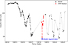 |
Fig. 1. Light curve of 2022 outburst of SAX J1808 in 0.5–10 keV energy band, using 1 ks bins. NICER observations are shown in black, and XMM-Newton observations are given in red. The blue star marks the epoch of the HST/STIS observation (2022 September 10). We rescaled the XMM-Newton count rate to the NICER count rate using a conversion factor of 1.44, which was calculated with the WebPIMMS tool (https://heasarc.gsfc.nasa.gov/cgi-bin/Tools/w3pimms/w3pimms.pl), and a power-law model with a photon index of Γ = 2.04 (Table 2). |
SAX J1808 was also the first AMSP to show coherent pulsations at optical and UV wavelengths during the rising and final stages of its 2019 outburst, respectively (Ambrosino et al. 2021). The observed highly pulsed optical and UV luminosities ( erg s−1,
  erg s−1) exceeded the values expected in the case of cyclotron emission from accretion columns by roughly 50 − 100 times, and the expected thermal output at those wavelengths by several orders of magnitude. Optical and UV pulsations have also been detected from the transitional millisecond pulsar PSR J1023+0038 (Ambrosino et al. 2017; Papitto et al. 2019; Jaodand et al. 2021; Ambrosino et al. 2021; Miraval Zanon et al. 2022), and from the redback PSR J2339-0533 (Papitto et al. 2025). In the former case, the high optically pulsed luminosities observed required a nonstandard interpretation in terms of synchrotron emission from the interface between the relativistic wind of a rotation-powered pulsar and the accretion flow (Papitto et al. 2019; Veledina et al. 2019; Baglio et al. 2023, 2025). However, this scenario assumes that the NS is active, as a rotation-powered pulsar and cannot apply to SAX J1808, where simultaneous X-ray pulsations indicate that the accretion flow extends down to the NS surface. The origin of the pulsed optical and UV emission in SAX J1808 thus remains uncertain.
In this paper, we report on a 125 ks-long XMM-Newton observation and a simultaneous 2.2 ks Hubble Space Telescope (HST) observation, performed during the reflaring stage of the outburst observed in SAX J1808 in 2022 (Illiano et al. 2023b). XMM-Newton’s uninterrupted coverage enabled a high-resolution study of the spectral and temporal evolution of the source X-ray emission as its flux varies by roughly one order of magnitude down to a few 1034 erg s−1. The simultaneous HST observation allowed us to extend the range of mass-accretion rates at which UV pulsations have been studied by a factor of approximately two and to perform the first simultaneous study in X-ray and UV bands.
2. Observations
2.1. XMM-Newton
XMM-Newton (Jansen et al. 2001) observed SAX J1808 for 125 ks starting on 2022 September 9 at 14:22:09 (UTC) (Obs.ID. 0884700801, PI: A. Papitto), during the final stage of the outburst (see red points in Fig. 1). Figure 2 shows the background-subtracted 0.5–10 keV EPIC-pn light curve. We used the Science Analysis System (SAS; v20.0.0) to process and reduce the data. We barycentered the photon arrival times observed by XMM-Newton using the barycen tool, with the JPL DE-405 Solar System ephemerides and the source position derived by Bult et al. (2020). The EPIC-pn camera operated in timing mode to achieve the 29.5 μs temporal resolution needed to study source variability and minimize photon pile-up, and it was equipped with a thick filter. The effective exposure was reduced to 108.2 ks after excluding soft-proton flaring episodes, identified when the EPIC-pn 10–12 keV count rate exceeded 0.8 c s−1. In timing mode, spatial information along one of the optical axis was discarded to allow a faster readout. As a result, the source appears on the EPIC-pn detector as a bright strip rather than its usual circular shape. The maximum number of counts were recorded in pixels characterized by RAWX coordinates 37 and 38. EPIC-pn events were extracted from a 21-pixel-wide region (1 pixel ≃4.1′) around the source position, spanning from RAWX = 28 to 48. We estimated the background far from the source, in a three-pixel-wide region centered on RAWX = 4.
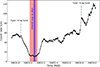 |
Fig. 2. Background-subtracted 0.5–10 keV XMM-Newton/EPIC-pn light curve of 2022 outburst of SAX J1808 measured using 200 s-long bins. A red band indicates the low-flux interval, and a blue band shows the interval of the HST observation discussed in this paper (see Sect. 3.2 for details). Two Type I X-ray bursts, detected at 59831.87 and 59832.82 MJD, are not plotted. Green dash-dotted lines indicate the epochs of their occurrence. |
During the XMM-Newton pointing, SAX J1808 exhibited two Type I X-ray bursts at MJD 59831.87 and 59832.82, which will be discussed in a dedicated upcoming publication. After obtaining the light curve, we created good time intervals (GTIs), discarding time intervals starting 10 s before and ending 150 s after each burst onset to perform spectral and timing analyses of the non-bursting emission. Following the recommended XMM-Newton/SAS procedures1, we extracted the source and background spectra from the cleaned event file, considering only single- and double-pixel events (PATTERN ≤ 4) and filtering out spurious events (FLAG = 0). We generated spectral response files using the tasks rmfgen and arfgen. The EPIC-pn spectra were rebinned using the SAS specgroup tool to have at least 25 background-subtracted counts per spectral channel and to sample the instrument’s resolution full width at half maximum with no more than three channels at any energy.
2.2. HST/STIS
The Space Telescope Imaging Spectrograph (STIS) on board HST observed SAX J1808 for 2.2 ks on 2022 September 10, starting at 02:05:41 (UTC) (GO/DD-17245, PI Miraval Zanon). The UV observation occurred during the interval of minimum X-ray flux, as shown by the blue band in Fig. 2. We removed an ∼400 s bump in the recorded flux at MJD 59832.103, which occurred when the observatory grazed the region of the South Atlantic Anomaly (HST help desk, private communication). The resulting UV light curve of the source observed with STIS is consistent with a constant count rate of ∼45 c s−1. The spectroscopic observation was performed in TIME-TAG mode, achieving a time resolution of 125 μs. The G230L grating, equipped with a 52 × 0.2 arcsec2 slit, provided a spectral resolution of ∼500 over the nominal (first-order) range. The total photon count rate was RHST = (46.62 ± 0.14) c s−1, with approximately 35% attributed to background radiation (BKGHST = (16.66 ± 0.09) c s−1).
We extracted the source photons across 19 slit channels (990 − 1010) and in the 165 − 310 nm wavelength range. This selection isolates the source signal, minimizes background contributions, and avoids noise arising from the G230L grating’s reduced response at the edges of the wavelength range. We estimated the background signal by selecting photons in the STIS slit channels outside the source region (200 − 900 and 1100 − 2000) in order to have high statistics and avoid the source contribution. We then averaged the resulting value and normalized it to the number of source slit channels. To analyze HST/STIS data, we first corrected the position of the slit channels using the Python custom-built external function stis_photons2. UV photon arrival times were then corrected to the Solar System barycenter (SSB) using the ODELAYTIME task (subroutine available in the IRAF/STDAS software package) and JPL DE200 ephemerides. Note that the difference between the JPL DE200 and DE405 ephemerides is negligible compared to the ∼1 s uncertainty on the absolute timing of the HST data (HST help desk, private communication).
2.3. NICER
We analyzed the Neutron star Interior Composition Explorer (NICER; Gendreau et al. 2012) observations obtained during the 2019 and 2022 outbursts and previously presented by Bult et al. (2020) and Illiano et al. (2023b). In 2019, NICER observed SAX J1808 from July 30 (MJD 58695) until November 8 (MJD 58795; ObsIDs 205026 and 258401). In 2022, we observed the source between August 19 (MJD 59810) and October 31 (MJD 59883; ObsIs 505026 and 557401). We processed and corrected the data according to the procedures described by Bult et al. (2020) and Illiano et al. (2023b). All data were processed using the standard NICER analysis software NICERDAS, part of HEASoft (v6.35.2). We processed the data using the nicerl2 task, selecting events in the 0.5 − 10 keV energy range. Photon arrival times for both datasets were corrected to the Solar System barycenter using the JPL DE405 ephemerides and the BARYCORR tool. We then adopted the source coordinates from Hartman et al. (2008) and Bult et al. (2020), respectively, for the 2019 and 2022 NICER datasets, to allow a direct comparison with the analyses presented by Bult et al. (2020) and Illiano et al. (2023b).
3. Coherent timing analysis
3.1. X-ray timing analysis
We performed a coherent timing analysis of the 2022 outburst of SAX J1808 using the XMM-Newton/EPIC-pn high-time-resolution dataset. We first corrected the photon arrival times for the Doppler delays introduced by the binary motion using the orbital parameters measured by Illiano et al. (2023b) from the pulse-timing analysis of 2022 NICER data. We created pulse profiles by epoch folding 1000 s time intervals in 16 phase bins around the best available estimate of the spin frequency (νF = 400.975209557 Hz from Illiano et al. 2023b). We adopted a bin length of 1000 s to ensure adequate statistics to detect the pulsation and track its amplitude and phase variations (see Fig. 4). Two harmonic components at most are usually required to satisfactorily model the pulse profile of SAX J1808 during such short intervals (see, e.g., Hartman et al. 2008), justifying the choice of sampling it in 16 phase bins. Only statistically significant pulse profiles were selected, namely folded profiles with a ratio between the sinusoidal amplitude and the corresponding 1σ error equal to or greater than three. The second panel of Fig. 4 shows the fractional amplitudes of the first and second harmonic. We focused the analysis of this work on the former, as it is significantly stronger. During the minimum of the X-ray flux (MJD 59832.02 to 59832.14; see the red band in Fig. 2), the amplitude of the fundamental (black dots) roughly doubled up to a value of ∼10%. Figure 3 shows the X-ray pulse profiles obtained by epoch by folding the high and low-flux intervals (red band in Fig. 2) of the XMM-Newton observation separately.
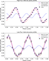 |
Fig. 3. X-ray pulse profiles obtained by folding the high- and low-flux intervals of XMM-Newton observation into 16 phase bins at a spin frequency of νF = 400.975209557 Hz. The solid line represents the best-fit model (constant plus two harmonics), while the dashed red and blue lines indicate the first and second harmonic contributions, respectively. For clarity, two cycles are shown. |
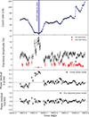 |
Fig. 4. Top panel: 0.5–10 keV XMM-Newton/EPIC-pn light curve using 1 ks bins, with Type I X-ray bursts removed. The dashed blue line shows the spline interpolation obtained with the UnivariateSpline function from scipy.interpolate. The blue band indicates the interval of the HST observation discussed in this paper (see Sect. 3.2 for details). Second panel: Pulse fractional amplitude for the first harmonic (black dots) and the second harmonic (red dots). Third and fourth panels: Phase residuals relative to a linear model and a model that includes a phase-flux correlation term, respectively. Note that, where not visible, the error bars are smaller than the data points. |
We first modeled the evolution of the pulse phase measured over the first harmonic using the following relation (e.g., Burderi et al. 2007; Sanna et al. 2022b; Papitto et al. 2007):
 (1)
(1)
Here, T0 is the reference epoch for the timing solution, ϕ0 is the pulse phase at T0, Δν = ν(T0)−νF represents the difference between the frequency at the reference epoch and the spin frequency used to epoch-fold the data, and  is the average spin-frequency derivative. The term Rorb models the phase residuals arising from differences between the adopted orbital parameters and the actual ones (see, e.g., Deeter et al. 1981). We first considered a constant frequency model (
 ), obtaining a value of ν(T0) that was not compatible with that expected according to the timing solution reached by Illiano et al. (2023b) (see Table 1).
Timing solution for SAX J1808 during 2022 outburst.
Best-fit parameters of XMM-Newton EPIC-pn 1.0–10 keV spectra of SAX J1808 during the high- and low-flux intervals.
Adding a spin frequency derivative term to the model reduced the residuals (Δχ2 = 339 for one degree of freedom less), but the modeling remained statistically unsatisfactory (χr2 = 11.86 over 91 degrees of freedom). The residuals with respect to either a linear or a quadratic model show large deviations (see the third panel of Fig. 4). This phenomenon often affects the evolution of the pulse phase of AMSPs and is commonly referred to as timing noise (Burderi et al. 2006; Papitto et al. 2007; Hartman et al. 2008, 2009; Patruno et al. 2009b). Timing noise is characterized by phase variations with amplitudes of up to several tenths of a cycle, affecting the measurement of the pulse frequency and its derivative. Here, a large phase jump of ∼0.4 cycles occurring around 59832 MJD, on a timescale of a few hours, was the most evident feature (see Fig. 4). This jump coincides with a decrease in the X-ray flux of the source by a factor of approximately three. When the flux returned to the initial values, the pulse phase also reverted to the estimates obtained before the jump.
To account for the phase shifts, we added a term describing a correlation between the X-ray flux and the pulse phase to Eq. (1), Rflux(t), which is possibly related to hot spot drifts (Patruno et al. 2009b):
 (2)
(2)
Following Bult et al. (2020), we used Rflux(t) = b (FX/F0)Λ, with FX being the X-ray bolometric flux, approximated by the 0.5–10 keV count rate for simplicity, and F0 the initial flux value at t = T0. To apply such a model, we interpolated the light-curve data using the UnivariateSpline function (available in Python’s scipy.interpolate library), as done by Illiano et al. (2023b). This method allows the flux values to be interpolated at the exact time points where phase data are available. The estimates of the X-ray flux so obtained (plotted with a dashed blue line in the top panel of Fig. 4) were used in Eq. (2) to fit the pulse phases, obtaining the residuals shown in the bottom panel of Fig. 4. By adding this flux-phase correlation term, we obtained a reduced χ2 of 1.82 for 90 degrees of freedom (d.o.f.), showing a highly significant improvement over the quadratic phase model (Δχ2 = 915 for the addition of one free parameter), with a probability of ∼1.5 × 10−38 of it being due to chance, according to an F-test. The best-fitting parameters of the flux-phase correlation term are  and Λ = −0.17(9). Even though the χ2 value obtained is still formally statistically unacceptable, the phase residuals no longer showed the phase jump, nor did they indicate the presence of significant structures or trends (Fig. 4, bottom panel). Unlike the linear and quadratic models, the value of the spin frequency obtained from the flux-adjusted model (Table 1) was consistent within the errors with that expected according to the timing solution reported in Illiano et al. (2023b), thus supporting the validity of the corrected model.
To estimate the uncertainties on the parameters b and Λ, we considered the contour levels of the fit χ2, χmin2 + 2.3, and χmin2 + 4.61 (Fig. 5), corresponding to confidence levels of 68% and 90%, respectively, for a fit with two free parameters of interest (Lampton et al. 1976; Avni 1976; Yaqoob 1998). The shape of the contour plots strongly suggests a correlation b × Λ ≃ const between the fit parameters.
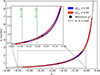 |
Fig. 5. Contour levels of χ2 obtained by varying both parameters b and Λ in the flux-adjusted phase fit. The contour levels are shown for χmin2 + 2.3 (blue) and χmin2 + 4.61 (red), corresponding to confidence levels of 68% and 90%, respectively, for a fit with two parameters (Lampton et al. 1976). The black dot indicates the values of b and Λ corresponding to the minimum χ2, while the dashed black line represents the contour corresponding to the constant value given by the product b × Λ. |
For comparison, we applied the same coherent timing technique to investigate the phase evolution of NICER data collected during the 2019 and 2022 outbursts. To avoid introducing significant uncertainties into the spline function, we filtered out data from the end of the outburst when the temporal gaps between consecutive observations exceeded three days. In both datasets, a flux-adjusted phase model again provided a better description of the observed phases than a linear or quadratic modeling. We obtained  and Λ = −0.14(5) for the 2019 dataset, and
  and Λ = −0.37(14) for the 2022 observation. The values of Λ are consistent, within uncertainties, with the value derived from the XMM-Newton timing analysis. These results are consistent with those of Bult et al. (2020), where Λ was fixed at −1/5. In contrast, the discrepancy with the values reported by Illiano et al. (2023b) arises from the different time interval considered for the phase fitting.
Figure 6 shows the fractional pulse amplitudes in seven energy bands, computed in the low-flux phase of the XMM-Newton light curve (top panel), and in the high-flux phase of the X-ray emission (bottom panel).
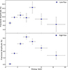 |
Fig. 6. Fractional amplitude of fundamental harmonic of X-ray pulse profiles in seven energy bands (0.5–1, 1–2, 2–3, 3–4, 4–5, 5–7, 7–10 keV) for the low-flux part of the light curve (top panel) and for the high-flux emission (bottom panel). |
The morphology we observed closely matches interval 4 of Bult et al. (2020) (see their Fig. 2), corresponding to the reflare phase of the 2019 outburst, which shows the highest amplitudes and a fractional amplitude that increases with energy before returning to near-initial values at ∼10 keV. The amplitudes we observed are generally higher than those reported by Bult et al. (2020), although the relative increase in pulsed fraction from ∼1 keV to 2–3 keV is consistent across the two outbursts, both showing an increase of approximately 40% relative to the initial values.
To compare the properties of the X-ray and UV pulsations, we measured the X-ray pulse amplitude in an interval strictly simultaneous to the HST observations (marked by a blue band in Fig. 4). In that interval, we obtained AX = (9.9 ± 0.8)%. The 0.5–10 keV flux measured in that time interval using a spectral model described in Table 2 was  . The pulsed 0.5–10 keV X-ray luminosity was then evaluated as
  , where d3.5 is the distance to the source in units of 3.5 kpc (Galloway & Cumming 2006).
3.2. UV timing analysis
To measure the spin period observed during the 2.2 ks-long HST/STIS observation, we performed an epoch folding search using m = 8 phase bins and a period resolution of δPHST, EFS = P2/2mTobs = 1.7 × 10⁻¹⁰ s, where Tobs is the total exposure time of the HST observation. We thus obtained a best-fitting period of PHST, EFS = 2.4939194(6)×10−3 s. Following Leahy (1987), the 1σ uncertainty reported was calculated using the following equation: σP = (P2/2 Tobs) ⋅ 0.71(χmax2/m − 1)−0.63, where the maximum of the χ2 value was found to be χmax2 ≃ 26.6. The period inferred from UV data is consistent, within uncertainties, with that obtained from X-ray data. We then folded the HST data at the best spin period. A single sinusoidal component describes the resulting UV pulsed profiles well, and an additional harmonic is not statistically justified, as it does not significantly improve the fit chi-square (see Fig. 7). To take the background into account, we evaluated a correction factor as Nγ(tot)/(Nγ(tot) − Nγ(bkg))≃1.556(5), where Nγ(tot) is the total number of detected photons and Nγ(bkg) the number of background photons. After applying this correction, the root-mean-square (r.m.s.) amplitude resulted as  .
.
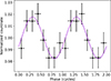 |
Fig. 7. Pulse profile obtained by folding the whole HST/STIS observation (GO/DD-17245, PI Miraval Zanon) into eight phase bins at a spin frequency of νF = 400.975209557 Hz. The solid line represents the best-fit model, consisting of a single sinusoidal component. For clarity, two cycles are shown. |
4. X-ray spectral analysis
We analyzed the X-ray spectral evolution of SAX J1808 during the outburst’s flaring stage by measuring the hardness ratio (HR), which is defined as the ratio of the count rates observed in the (2–10 keV) and (0.7–2 keV) energy bands. Panels (a) and (b) of Fig. 8 show the variation of the HR over time and intensity, respectively. The source emission significantly softened during the phase of minimum X-ray count rate. The continuous decrease in the HR reached a minimum when the source flux was at its lowest. The HR then returned to its initial value, following the trend of the light curve.
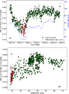 |
Fig. 8. Panel (a): Evolution of HR of SAX J1808 during XMM-Newton observation of reflare phase of 2022 outburst. The HR was estimated from the (2–10 keV)/(0.7–2 keV) energy band. For comparison, the XMM-Newton light curve is shown in blue in the background. Panel (b): Hardness-intensity diagram (HID) of SAX J1808 obtained using XMM-Newton EPIC-pn observation and 200 s bins. The intensity is given in counts per second. The points corresponding to the minimum of the source X-ray flux on the light curve, between 59832.02 MJD and 59832.14 MJD, are marked in red. |
To investigate the softening of the emission, we extracted spectra considering both the low-flux phase of the light curve (between 59832.02 MJD and 59832.14 MJD; see the red band of Fig. 2 and corresponding red data points in Fig. 8) and the high-flux emission, obtained by excluding the entire low-flux interval and its rise and decay phases; i.e., from MJD 59831.88 to 59832.23. We performed the spectral analysis using the X-ray spectral fitting package HEASARC XSPEC (Arnaud 1996) version 12.14.0. We used TBabs to model the interstellar photoelectric absorption, with the chemical abundances of Wilms et al. (2000) and the cross-sections reported in Verner et al. (1996). To avoid the impact of calibration uncertainties at low energies, we excluded data below 1 keV from the EPIC-pn spectral analysis3. Following previous works, we fixed the equivalent hydrogen column density at 0.21 × 1022 cm−2 (Papitto et al. 2009; Di Salvo et al. 2019). We first modeled the 1–10 keV spectrum observed in the high-flux interval with a blackbody component, bbodyrad, and a thermal Comptonization component, nthComp (Zdziarski et al. 1996; Zycki et al. 1999). This spectral decomposition is commonly used to model the broad-band continuum emission in AMSPs (Poutanen 2006; Di Salvo & Sanna 2022). The parameters of the thermal Comptonization continuum model are the asymptotic power-law photon index, Γ; the hot, Comptonizing electron temperature, kTe; and the seed photon temperature, kTseed. We set the inp_type parameter to zero, indicating that the seed photons are distributed as a blackbody. Since no high-energy cut-off was observed in the XMM-Newton spectrum, we fixed kTe to 30 keV (see, e.g., Di Salvo et al. 2019). This choice had no significant impact on the obtained results. Using this model, we obtained an unacceptably high reduced χ2 of 6 for 146 d.o.f.. The residuals shown in the middle panel of Fig. 9 suggest the presence of a reflection component. We therefore convolved the nthComp component with the rfxconv model from Done & Gierliński (2006) and the relativistic blurring kernel rdblur (Fabian et al. 1989). The parameters of the reflection model are the relative reflection normalization, the iron abundance relative to the solar one, the ionization parameter of the disk’s log ξ, the inner- and outer-disk radii, the disk inclination, and the emissivity index, β, which describes the emissivity of the illuminated disk as a function of the emission radius (∝rβ). We first allowed the iron abundance to vary, but as this did not produce a significant decrease in the fit’s χ2, we fixed it at 1. Given the limited spectral coverage and the weakness of the reflection features, we fixed the reflection fraction (rel_refl) at −0.62, consistent with the value found in previous studies (Di Salvo et al. 2019). We also accounted for residual emission features evident in the soft-energy part of the spectrum by introducing three Gaussian components. Some of these features are listed in the official XMM-Newton user guide4 as known instrumental lines (the Si-K line at 1.84 keV and the Au-M line at 2.2 keV). We also observed an emission line at 3.5 keV, which we attributed to Ar XVIII fluorescence (see, e.g., Pintore et al. 2016 and Malacaria et al. 2025). In some cases, the spectral resolution of the XMM-Newton/EPIC-pn instrument was insufficient to constrain the width of the modeled lines. Therefore, we fixed the σ parameter to 0 keV. The resulting model gave a reduced χ2 of 1.26 with 142 d.o.f. Figure 9 shows the model and the residuals (bottom panel), while Table 2 lists the best-fit parameters.
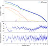 |
Fig. 9. XMM-Newton/EPIC-pn spectrum (1.0–10 keV) of high-flux emission from SAX J1808 (top) and best-fit model plotted with a solid line and given in Table 2. The fit model is TBabs*(bbodyrad + gaussian + gaussian + gaussian + nthComp + rdblur*rfxconv*nthComp). The model components are also plotted as dashed lines: the blackbody component, bbodyrad, in red; the Comptonization component, nthcomp, in green; the reflection component in orange; and the Gaussians in purple and yellow. The bottom panel displays the residuals relative to the best-fit model, while the middle panel shows the residuals from a fit performed without the reflection component. |
We then modeled the spectrum of the low-flux part of the light curve in the 1–10 keV energy band. We adopted the same spectral model used for the high-flux emission, but without the Gaussian components that described the low-energy emission features, which were not detectable in this spectrum, likely due to lower statistics. Figure 10 shows the model and the residuals, resulting in a reduced χ2 of 1.19 with 134 d.o.f. The best-fit parameters are reported in Table 2.
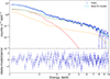 |
Fig. 10. XMM-Newton/EPIC-pn spectrum (1.0–10 keV) of low part of light curve of SAX J1808 (top) and residuals with respect to best-fit model plotted with a solid line and given in Table 2. The fit model is TBabs*(bbodyrad + nthComp + rdblur*rfxconv*nthComp). The model components are also plotted as dashed lines, with the same color-coding as in Fig. 9. |
5. Spectral energy distribution
Figure 11 shows the UV spectrum of SAX J1808, covering the wavelength range of 1650−3100 Å. The only notable feature is a possible weak absorption line near 2600 Å, most likely due to Fe II.
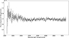 |
Fig. 11. UV spectrum of HST/STIS observation of SAX J1808 performed on September 10, 2022 and binned at 5 Å in the 1650−3100 Å wavelength range. |
We corrected the UV spectrum for interstellar extinction using the empirical relation AV = NH/(2.87 ± 0.12)×1021 cm−2 (Foight et al. 2016), where NH = 2.1 × 1021 cm−2 represents the hydrogen column density along the line of sight to SAX J1808 (Di Salvo et al. 2019), which gives AV ≃ 0.73 mag. We obtained a corresponding reddening of E(B − V)≃0.27 using the extinction coefficients of Schlafly & Finkbeiner (2011) for RV = 3.1. We then applied the extinction law of Fitzpatrick (1999) to compute Aλ across the STIS spectral range and corrected each wavelength bin with the corresponding extinction value to derive the dereddened spectrum. We numerically integrated the spectrum with the trapezoidal rule, which approximates the area under the curve by dividing it into small trapezoids, obtaining a UV-flux value of FUV = (3.7 ± 0.7)×10−12 erg cm−2 s−1. Considering the measured UV pulse amplitude (see Sect. 3.2), the coherent UV pulses detected during the HST/STIS observation showed a pulsed luminosity of  .
.
Figure 12 shows the spectral energy distribution (SED) of the total and pulsed emission of SAX J1808 in the UV and X-ray bands during the September 10, 2022 simultaneous observations. To evaluate the X-ray pulsed flux simultaneously with the HST observations, we measured the r.m.s. amplitude in seven energy bands (Fig. 6) and multiplied these values for the unabsorbed X-ray fluxes calculated over the same energy ranges. We then scaled the resulting values by the ratio between the mid-point energy of the interval and the width of the energy interval to convert the pulsed X-ray fluxes into νFν units.
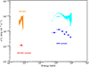 |
Fig. 12. Unabsorbed SED of SAX J1808 from UV to X-rays obtained using simultaneous XMM-Newton/HST (STIS) observations performed during the 2022 outburst reflare phase (September 10, 2022). The HST spectrum is shown in orange from 165 to 310 nm. The pulsed UV flux is plotted with a red triangle. The total 0.5–10 keV X-ray fluxes observed by XMM-Newton are plotted using light blue points. The pulsed X-ray fluxes, plotted as dark blue squares, are calculated over the 0.5–1, 1–2, 2–3, 3–4, 4–5, 5–7, and 7–10 keV energy bands. |
6. Discussion
6.1. Phase shifts and hot-spot displacements
We analyzed an uninterrupted XMM-Newton observation of the AMSP SAX J1808 performed during the final reflaring stage of the 2022 outburst. X-ray coherent pulsations were detected throughout the observation, providing strong evidence for channeled accretion onto the magnetic poles of the NS at very low X-ray luminosity. The 0.5–10 keV luminosity measured during the phase of minimum observed X-ray flux (red band in Fig. 2, Table 2) was  . This value is on the order of the lowest X-ray luminosity at which pulsations of SAX J1808 were previously observed (around a few ×1034 erg s−1; Hartman et al. 2008, 2009; Patruno et al. 2009a; Bult et al. 2019b; Archibald et al. 2015).
To estimate the location of the inner-disk radius during the observation, we used the relation  (Pringle & Rees 1972; Lamb et al. 1973; Campana et al. 2018), where μ = BR*3 ∼ 1026 G cm3 is the magnetic moment measured from the secular spin-down rate (Hartman et al. 2008), and Ṁ is related to the luminosity as Ṁ = LX R∗/GM∗. We estimated the bolometric 0.1–100.0 keV X-ray luminosity during the low- and high-flux parts of the observations by extrapolating the best-fitting spectral model from the 1.0–10 keV range. We obtained
  and
and  , respectively. The corresponding estimates of the inner-disk radius are
  and
and  . Note that these uncertainties are likely underestimated, as they do not include contributions from uncertainties of the magnetic-field strength, mass, and radius. For comparison, the corotation radius of SAX J1808 is
  , where m1.4 is the NS mass in units of 1.4 M⊙. The observation of X-ray pulsations in the low-flux interval confirms that channeled accretion continues even when the mass-accretion rate is low and that the inner disk remains close to the corotation radius, likely in a weak propeller regime (Patruno et al. 2016). Notably, the X-ray pulsations showed a larger amplitude at the lowest observed fluxes (second panel of Fig. 4). This behavior has been observed in several AMSPs, where the pulsed fraction tends to increase as the accretion rate drops (see, e.g., IGR J17379-3747, MAXI J1957+032, MAXI J1816-195, IGR J17498-2921; Bult et al. 2019a, Sanna et al. 2022a, Bult et al. 2022, and Illiano et al. 2024).
A phase-coherent timing analysis revealed a clear phase jump of Δϕ ≃ 0.4 cycles, coincident with a decrease by a factor of three of the X-ray luminosity to the lowest value measured during our observation (LX(low) ≃ 1035 erg s−1). Timing noise is known to affect the phases observed from SAX J1808 (Hartman et al. 2008, 2009) and other AMSPs (Patruno et al. 2009b). Burderi et al. (2006) observed a phase shift of the opposite sign and roughly half an order of magnitude (Δϕ ≃ −0.2) during the 2002 outburst; this was simultaneous to a rapid drop of the X-ray flux and before the beginning of the reflaring phase. Several models have been proposed to explain such changes. Poutanen et al. (2009) and Ibragimov & Poutanen (2009) interpreted the phase shift and the appearance of a secondary peak at the end of the 2002 outburst in terms of the opening of the view to the antipodal spot due to the recession of the inner disk when the mass-accretion rate decreased. A related interpretation involves changes in the disk-magnetosphere coupling and emission geometry (Kajava et al. 2011). However, in our observation, no secondary peak appeared when the X-ray flux dropped. Instead, the amplitude of the second harmonic became weaker, while the first harmonic became twice as strong compared to the higher flux level (see Figs. 3 and 4). Assuming the drop of the X-ray flux causes an increase in Rin, the lack of a strong secondary peak suggests that the disk was already sufficiently far from the NS to avoid significantly occulting the secondary pole. Indeed, the observed X-ray flux (≲1.5 × 10⁻¹⁰ erg cm−2 s−1; 0.5–10 keV) was lower than the typical flux at which the transition to the rapid drop occurred in 2002 (≳10−9 erg cm−2 s−1). An alternative explanation involves scattering of the hot-spot emission in the accretion funnel (Ahlberg et al. 2024), but this effect is only relevant at higher accretion rates (Ṁ ≳ 10−10 Ṁ yr−1) than those observed in our observation.
Another possible explanation for the observed phase shifts in AMSPs involves spot movement in the azimuthal direction (Lamb et al. 2009; Kulkarni & Romanova 2013). In particular, variations in the hot-spot longitude directly affect the pulse arrival times. Such drifts can result from changes in the mass-accretion rate. As the accretion disk recedes, the inflowing matter couples to different magnetic-field lines and is channeled to slightly displaced regions on the NS surface. The largest phase variation we observed in the XMM-Newton data taken during the reflaring stage of the 2022 outburst corresponds to a shift in the hot-spot longitude of ≃100°. Patruno et al. (2009b) first proposed the existence of a correlation between the observed pulse phase and the X-ray flux, based on the improvement it produced in the description of the phase evolution of a sample of AMSPs. Thus, to account for the phase shifts observed in our analysis, we added a phase-flux correlation term to the constant frequency model, Rflux(t) = b (FX/F0)Λ, as in Bult et al. (2020). This addition yielded a significant improvement in the description of the temporal evolution of the observed pulse phases. The value of Λ = −0.17(9) we obtained agrees with the value suggested by numerical simulations of accretion onto a rapidly rotating NS (Kulkarni & Romanova 2013). These simulations suggest that the azimuthal position of the hot spot relative to the magnetic pole scales proportionally with the magnetospheric radius, δϕ ∝ Rm. Assuming  and Ṁ to be proportional to the bolometric flux, we obtain δϕ ∝ Rm ∝ FXΛ. The value we found is compatible with the index Λ = −1/5, which we found by defining the inner-disk radius as the point where the inflowing matter is forced into corotation with the NS magnetosphere (Spruit & Taam 1993; D’Angelo & Spruit 2010). An even steeper dependence of approximately the usual definition of the Alfvén radius, Λ = −2/7, cannot be excluded, however.
The contour plot in the (b, Λ) plane reveals a correlation between these two parameters, b ⋅ Λ ≃ const (dashed black line in Fig. 5). Such a correlation likely arose because the fit was primarily driven by the step-like variation of Δϕ ≃ 0.4 in response to a variation in the flux Δ FX ≃ 50 c s−1, with a similar shape. Consequently, the fit was mainly sensitive to the ratio Δϕ/ΔFX ≃ 8 × 10⁻³ s, which approximates the derivative of the functional form of the phase-flux correlation, dϕ/dFX = bΛ ⋅ F0 ⋅ (FX/F0)Λ − 1 ∼ b ⋅ Λ. Observations of a few phase jumps of variable amplitude, simultaneous to flux variations of different magnitudes, would provide a stronger test of the model and likely remove the degeneracy.
Analysis of NICER observations from the 2019 and 2022 outbursts yielded consistent values of Λ within the uncertainties. Whereas for the 2019 dataset Bult et al. (2020) fixed the Λ index to the theoretically expected value of −1/5, we treated Λ as a free parameter, obtaining Λ = −0.14(5). Our analysis of 2022 data gave a value of Λ = −0.37(14), which differs from that reported by Illiano et al. (2023b) (Λ = −0.81(12)). Such a difference is due to our decision not to consider the phase evolution after the first long gaps in data, as these would have prevented us from reliably approximating the flux with a spline function.
When the accretion disk recedes toward the end of an outburst, the spot latitude is also expected to change as matter is channeled toward the NS surface by magnetic lines that land closer to the magnetic pole. Such variations modify the amplitude of the harmonic components of the pulsed profile (Poutanen & Beloborodov 2006; Lamb et al. 2009). In particular, if the hot spot is close to the stellar spin axis, modest changes in its latitude can produce significant variations. The effect of such changes on the observed pulsed fraction depends on the initial spot latitude (see Fig. 1 from Lamb et al. 2009 and Fig. 6 from Poutanen & Beloborodov 2006). If only a single spot is visible, a decrease in the spot latitude generally reduces the pulsed fraction. On the other hand, if two antipodal spots are visible and the primary spot latitude is ≳45°, its decrease might produce an increase in the fractional amplitude. Simultaneous to the flux decrease and the phase shift discussed above, we observed an increase in the amplitude of the fundamental frequency up to ≃10% (second panel of Fig. 4). Such an increase in the pulsed fraction might thus be interpreted in terms of a change in the spot latitudes caused by a receding inner disk, provided that SAX J1808 is an approximately orthogonal rotator whose pulse profile arises from two spots. In such a geometry, the presence of two nearly antipodal hot spots is also expected to enhance the polarimetric signature. This effect was recently observed by IXPE in the orthogonal rotator GRO J1008−57 (Tsygankov et al. 2023), suggesting that similar measurements of SAX J1808 could provide additional constraints on its geometry.
6.2. UV pulsations
We presented a timing analysis of an HST/STIS UV observation performed simultaneously with the interval of minimum X-ray flux observed by XMM-Newton (Fig. 2). We confirmed the significant detection of UV pulsations, with a pulsed luminosity of  consistent with that observed during the previous accretion event of SAX J1808 in 2019 (Ambrosino et al. 2021).
In both the 2019 and 2022 outbursts, UV pulsations were detected during the reflaring phase (see our Fig. 2 and Fig. 1 of Ambrosino et al. 2021), across an X-ray luminosity range spanning a factor of ∼2 (see Table 3). The values of the pulsed X-ray and UV luminosity we observed simultaneously in the 2022 outburst (see Table 3) give a ratio of  . Applying the same analysis to the non-simultaneous 2019 observations yields a similar ratio of 48 ± 18.
Total and pulsed luminosities in X-ray and UV bands computed for the 2019 and 2022 outbursts.
Standard mechanisms hardly explain the very bright, pulsed optical and UV flux of SAX J1808. In fact, the observed values imply a brightness temperature of > 1 MeV for a 10 km-wide NS at the distance of SAX J1808, which can be safely excluded given the flux observed in the X-ray band (Ambrosino et al. 2021). On the other hand, the thermal emission observed at soft X-rays is expected to produce a 165–310 nm UV luminosity of
 (3)
(3)
where kB is the Boltzmann constant, kTbb is the blackbody temperature, A ≈ πR*2(R*/Rco) is the hot-spot area of the accreting polar cap (∼100 km2 if the whole NS is involved; Frank et al. 2002), and ν1 and ν2 represent the lower and upper frequency limits of the UV band. Using kTbb = 0.362 keV (Table 2), the expected UV luminosity is ∼8 × 1027 erg s−1, which is four orders of magnitude lower than observed. On the other hand, cyclotron emission from hot electrons in the post-shock region of the accretion columns of a 3.5 × 10⁸ G magnetic-field pulsar can account for a UV luminosity up to ≃6 × 1029 erg s−1 (Ambrosino et al. 2021), which is lower by a factor of 150 than the value reported here. Even assuming extreme beaming, it seems highly unlikely that such processes can account for the brightness of the UV pulsations observed from SAX J1808.
The transitional millisecond pulsar PSR J1023+0038 is the only other millisecond pulsar known to show both UV and optical pulsations (Ambrosino et al. 2017; Papitto et al. 2019; Ambrosino et al. 2021; Jaodand et al. 2021; Miraval Zanon et al. 2022). These signals were detected when the source was in an X-ray-faint (LX ≃ a few × 1033 erg s−1) accretion-disk regime. The SED of the pulsed flux of PSR J1023+0038 was compatible with a power-law relation connecting the optical and UV to the X-ray band (Papitto et al. 2019; Miraval Zanon et al. 2022). Recently, Baglio et al. (2025) showed that the SED of polarized emission also follows a compatible trend. Synchrotron emission from electrons accelerated where the rotation-powered electromagnetic wind of the pulsar interacts with the mass inflow has been proposed to explain the high pulsed luminosity observed at optical and UV energies (Papitto et al. 2019; Veledina et al. 2019; see also Illiano et al. 2023a; Baglio et al. 2023). Unlike the case of PSR J1023+0038, the simultaneous estimates of the pulsed X-ray and UV fluxes of SAX J1808 cannot be connected by a single power law (see Fig. 12), arguing against an interpretation in terms of a standard synchrotron-emission process. Most importantly, the observed X-ray luminosity of SAX J1808 (LX ≃ a few × 1035 erg s−1) ensures that the system is accretion powered and that high-density plasma engulfs the magnetosphere. Ambrosino et al. (2021) suggested the possibility of a coexistence or a fast alternation between optical and UV pulsed radiation produced by electrons accelerated by a rotation-powered pulsar and X-ray pulsed emission driven by mass accretion onto the polar caps of the NS. While future theoretical investigation will assess the feasibility of such an unusual scenario, an immediate explanation of the high pulsed luminosity of SAX J1808 that does not rely on strong beaming of the pulsed flux is lacking.
6.3. Evolution in the X-ray spectrum
A study of the evolution of the HR of the source during the XMM-Newton observation revealed a softening of the emission corresponding to the minimum of the source’s X-ray flux. To investigate the origin of this behavior, we performed spectral analysis of both the high- and low-flux intervals of the light curve. The spectra were fit with a model consisting of a blackbody component, a Comptonization component, and a reflection component. Most of the best-fit parameters obtained for the high- and low-flux intervals are consistent at the 3σ confidence level. The normalization of the Comptonization component was the only parameter that decreased significantly in the low-flux interval. The normalization of the bbodyrad component, instead, shows only a slight variation, barely reaching the 3σ confidence level. The ratio between the flux in the Comptonization and blackbody components (see Table 2) changed from  in the high-flux state to 2.3 ± 0.4 in the low-flux state. Such a behavior could be related to the different physical origins of the two components: the thermal blackbody emission likely originates from a fraction of the NS surface; while the Comptonization emission arises from up-scattering of these same seed photons by electrons in the accretion columns (Poutanen 2006). A decrease in mass accretion rate might then reduce the efficiency of the Comptonization process faster than it affects the thermal blackbody emission, possibly leading to a softer spectrum at lower fluxes.
The parameters measured for the soft and reflection components can provide constraints on the geometry of the emitting regions. The normalization of the bbodyrad component can be used to estimate the radius of the emitting blackbody region,  , where D10 = 0.35 is the distance to the source in units of 10 kpc (Galloway & Cumming 2006). We thus obtained
  for the high-flux emission spectrum and Rbb = 2.86 ± 0.14 km for the low-flux part of the light curve. The blackbody component can be interpreted as unscattered emission from a portion of the NS surface. Interestingly, the region appears smaller at lower flux values, possibly suggesting a shrinkage of the emission region. The best-fit parameters of the rdblur convolution model of the high-flux spectrum returned an estimate for the inner-disk radius of Rin < 6.7 Rg (in units of the gravitational Schwarzschild radius Rg = GM/c2), and
  for the inclination. The inner-disk radius is equivalent to values of < 14 km for a NS mass of 1.4 M⊙, which is consistent with the inner disk being truncated before the NS surface and inside the corotation boundary. However, the Rin value inferred from the reflection model appears smaller than expected if the disk is truncated near the corotation radius, as might be suggested by the observed low flux (see Sect. 6.1 for further discussion). Both the inner radius and inclination are consistent with previous estimates based on the relativistic broadening of the reflection features of this source (Papitto et al. 2009; Cackett et al. 2009; Di Salvo et al. 2019). An optical estimate based on quiescent light-curve modeling yields a lower inclination of
  degrees (Wang et al. 2013). Such a low inclination would imply an unusually low NS mass to satisfy the companion’s radial-velocity constraints. This would, in turn, exacerbate the tension with the higher inclination required by the X-ray reflection analysis (see Sect. 4.3 of Di Salvo et al. 2019 for further discussion). The uncertainties on the reflection parameters are coarser. This hampers the detection of a change in the inner-disk radius, as suggested by the variation in pulse amplitude and phase.
7. Conclusions
We investigated the temporal and spectral properties of simultaneous X-ray and UV pulsations from the AMSP SAX J1808. We analyzed XMM-Newton and HST observations obtained at low accretion rates during the final reflaring stage of its 2022 outburst. The main results are as follows.
-
We detected significant X-ray pulsations down to a luminosity of
 in the 0.5–10 keV band. This value is of the order of the lowest X-ray luminosities at which X-ray pulsations have ever been detected in this source (approximately a few 1034 erg s−1; Bult et al. 2019b).
 -
XMM-Newton data revealed significant variations in both pulse phase and amplitude. In particular, a distinct phase jump of approximately 0.4 was observed, coinciding with an amplitude increase up to ∼10% and a decrease in X-ray flux to the lowest luminosity reached during our observation. We interpret these shifts as the drift of emission regions in longitude and latitude on the NS surface as a function of the mass-accretion rate.
-
To take into account the phase shifts, we modeled the phase delays using the flux-adjusted model (Bult et al. 2020), obtaining an index of correlation between the phases and the X-ray flux of Λ = −0.17(9). This value matches the expected scaling of the magnetospheric radius with the accretion rate, which is predicted to be −1/5 from numerical simulations of accretion onto a rotating NS (Kulkarni & Romanova 2013).
-
During the X-ray flux minimum, simultaneous HST observations confirmed significant UV pulsations. The pulsed UV luminosity (
 ) was consistent with that observed during the 2019 outburst. In addition, the pulsed X-ray-to-UV luminosity ratio remained consistent across the two outburst events. The SED of the pulsed emission cannot be explained by a single power-law or thermal model, challenging standard emission scenarios.
 -
Spectral analysis of high- and low-flux intervals of the XMM-Newton observation revealed a softening of the emission during the minimum of the X-ray source flux, associated with a decrease in the Comptonization component. The measured inclination (
 ) and the inner-disk radius (< 14 km, for a NS mass of 1.4 M⊙) remain consistent with previous measurements, supporting a truncated disk within the corotation radius.
Acknowledgments
We thank the referee for useful comments. This work is based on observations obtained with XMM-Newton, an ESA science mission with instruments and contributions directly funded by ESA Member States and NASA; the NASA/ESA Hubble Space Telescope obtained from the Space Telescope Science Institute (program GO/DD-17245), which is operated by the Association of Universities for Research in Astronomy, Inc., under NASA contract NAS 5–26555; NASA through the NICER mission and the Astrophysics Explorers Program. This work was supported by INAF (Research Grant ‘Uncovering the optical beat of the fastest magnetized neutron stars (FANS)’ and ‘Polarized X-rays from an accreting millisecond pulsar: a pathway to the equation of state of neutron stars (PULSE-X)’, PI: Papitto), the Italian Ministry of University and Research (MUR PRIN 2020) Grant 2020BRP57Z, ‘Gravitational and Electromagnetic-wave Sources in the Universe with current and next-generation detectors (GEMS)’, PI: Astone) and the Fondazione Cariplo/Cassa Depositi e Prestiti (Grant 2023-2560 ‘Taking the optical pulse of the quickest spinning Neutron Stars: a pilot exploratory study (SPES)’, PI: Papitto).
References
- Ahlberg, V., Poutanen, J., & Salmi, T. 2024, A&A, 682, A60 [NASA ADS] [CrossRef] [EDP Sciences] [Google Scholar]
- Alpar, M. A., Cheng, A. F., Ruderman, M. A., & Shaham, J. 1982, Nature, 300, 728 [NASA ADS] [CrossRef] [Google Scholar]
- Ambrosino, F., Papitto, A., Stella, L., et al. 2017, Nat. Astron., 1, 854 [NASA ADS] [CrossRef] [Google Scholar]
- Ambrosino, F., Miraval Zanon, A., Papitto, A., et al. 2021, Nat. Astron., 5, 552 [NASA ADS] [CrossRef] [Google Scholar]
- Archibald, A. M., Bogdanov, S., Patruno, A., et al. 2015, ApJ, 807, 62 [NASA ADS] [CrossRef] [Google Scholar]
- Arnaud, K. A. 1996, ASP Conf. Ser., 101, 17 [Google Scholar]
- Avni, Y. 1976, ApJ, 210, 642 [NASA ADS] [CrossRef] [Google Scholar]
- Baglio, M. C., Coti Zelati, F., Campana, S., et al. 2023, A&A, 677, A30 [NASA ADS] [CrossRef] [EDP Sciences] [Google Scholar]
- Baglio, M. C., Coti Zelati, F., Di Marco, A., et al. 2025, ApJ, 987, L19 [Google Scholar]
- Bhattacharya, D., & van den Heuvel, E. 1991, Phys. Rep., 203, 1 [NASA ADS] [CrossRef] [Google Scholar]
- Bult, P., Markwardt, C. B., Altamirano, D., et al. 2019a, ApJ, 877, 70 [Google Scholar]
- Bult, P. M., Gendreau, K. C., Arzoumanian, Z., et al. 2019b, ATel., 13001, 1 [Google Scholar]
- Bult, P., Chakrabarty, D., Arzoumanian, Z., et al. 2020, ApJ, 898, 38 [CrossRef] [Google Scholar]
- Bult, P., Altamirano, D., Arzoumanian, Z., et al. 2022, ApJ, 935, L32 [NASA ADS] [CrossRef] [Google Scholar]
- Burderi, L., Di Salvo, T., Menna, M. T., Riggio, A., & Papitto, A. 2006, ApJ, 653, L133 [NASA ADS] [CrossRef] [Google Scholar]
- Burderi, L., Di Salvo, T., Lavagetto, G., et al. 2007, ApJ, 657, 961 [NASA ADS] [CrossRef] [Google Scholar]
- Cackett, E. M., Altamirano, D., Patruno, A., et al. 2009, ApJ, 694, L21 [NASA ADS] [CrossRef] [Google Scholar]
- Campana, S., & Di Salvo, T. 2018, Astrophys. Space Sci. Libr., 457, 149 [NASA ADS] [CrossRef] [Google Scholar]
- Campana, S., Colpi, M., Mereghetti, S., Stella, L., & Tavani, M. 1998, A&ARv, 8, 279 [NASA ADS] [CrossRef] [Google Scholar]
- Campana, S., D’Avanzo, P., Casares, J., et al. 2004, ApJ, 614, L49 [NASA ADS] [CrossRef] [Google Scholar]
- Campana, S., Stella, L., Mereghetti, S., & de Martino, D. 2018, A&A, 610, A46 [NASA ADS] [CrossRef] [EDP Sciences] [Google Scholar]
- D’Angelo, C. R., & Spruit, H. C. 2010, MNRAS, 406, 1208 [NASA ADS] [Google Scholar]
- D’Angelo, C. R., & Spruit, H. C. 2012, MNRAS, 420, 416 [Google Scholar]
- Deeter, J. E., Boynton, P. E., & Pravdo, S. H. 1981, ApJ, 247, 1003 [NASA ADS] [CrossRef] [Google Scholar]
- Di Salvo, T., & Sanna, A. 2022, Astrophys. Space Sci. Libr., 465, 87 [Google Scholar]
- Di Salvo, T., Sanna, A., Burderi, L., et al. 2019, MNRAS, 483, 767 [NASA ADS] [CrossRef] [Google Scholar]
- Done, C., & Gierliński, M. 2006, MNRAS, 367, 659 [NASA ADS] [CrossRef] [Google Scholar]
- Fabian, A. C., Rees, M. J., Stella, L., & White, N. E. 1989, MNRAS, 238, 729 [Google Scholar]
- Finger, M. H., Bildsten, L., Chakrabarty, D., et al. 1999, ApJ, 517, 449 [NASA ADS] [CrossRef] [Google Scholar]
- Fitzpatrick, E. L. 1999, PASP, 111, 63 [Google Scholar]
- Foight, D. R., Güver, T., Özel, F., & Slane, P. O. 2016, ApJ, 826, 66 [Google Scholar]
- Frank, J., King, A., & Raine, D. J. 2002, Accretion Power in Astrophysics (Third Edition) [Google Scholar]
- Galloway, D. K., & Cumming, A. 2006, ApJ, 652, 559 [Google Scholar]
- Gendreau, K. C., Arzoumanian, Z., & Okajima, T. 2012, SPIE, 8443, 844313 [Google Scholar]
- Ghosh, P., & Lamb, F. K. 1979, ApJ, 232, 259 [Google Scholar]
- Hartman, J. M., Patruno, A., Chakrabarty, D., et al. 2008, ApJ, 675, 1468 [NASA ADS] [CrossRef] [Google Scholar]
- Hartman, J. M., Patruno, A., Chakrabarty, D., et al. 2009, ApJ, 702, 1673 [NASA ADS] [CrossRef] [Google Scholar]
- Ibragimov, A., & Poutanen, J. 2009, MNRAS, 400, 492 [CrossRef] [Google Scholar]
- Illarionov, A. F., & Sunyaev, R. A. 1975, A&A, 39, 185 [NASA ADS] [Google Scholar]
- Illiano, G., Papitto, A., Ambrosino, F., et al. 2023a, A&A, 669, A26 [NASA ADS] [CrossRef] [EDP Sciences] [Google Scholar]
- Illiano, G., Papitto, A., Sanna, A., et al. 2023b, ApJ, 942, L40 [NASA ADS] [CrossRef] [Google Scholar]
- Illiano, G., Papitto, A., Marino, A., et al. 2024, A&A, 691, A189 [NASA ADS] [CrossRef] [EDP Sciences] [Google Scholar]
- Illiano, G., Papitto, A., Campana, S., et al. 2026, A&A, 706, A52 [NASA ADS] [CrossRef] [EDP Sciences] [Google Scholar]
- Jansen, F., Lumb, D., Altieri, B., et al. 2001, A&A, 365, L1 [NASA ADS] [CrossRef] [EDP Sciences] [Google Scholar]
- Jaodand, A. D., Hernández Santisteban, J. V., Archibald, A. M., et al. 2021, arXiv e-prints [arXiv:2102.13145] [Google Scholar]
- Kajava, J. J. E., Ibragimov, A., Annala, M., Patruno, A., & Poutanen, J. 2011, MNRAS, 417, 1454 [NASA ADS] [CrossRef] [Google Scholar]
- Kulkarni, A. K., & Romanova, M. M. 2013, MNRAS, 433, 3048 [NASA ADS] [CrossRef] [Google Scholar]
- Lamb, F. K., Pethick, C. J., & Pines, D. 1973, ApJ, 184, 271 [NASA ADS] [CrossRef] [Google Scholar]
- Lamb, F. K., Boutloukos, S., Van Wassenhove, S., et al. 2009, ApJ, 706, 417 [NASA ADS] [CrossRef] [Google Scholar]
- Lampton, M., Margon, B., & Bowyer, S. 1976, ApJ, 208, 177 [Google Scholar]
- Leahy, D. A. 1987, A&A, 180, 275 [NASA ADS] [Google Scholar]
- Malacaria, C., Papitto, A., Campana, S., et al. 2025, A&A, 699, A288 [NASA ADS] [CrossRef] [EDP Sciences] [Google Scholar]
- Miraval Zanon, A., Ambrosino, F., Coti Zelati, F., et al. 2022, A&A, 660, A63 [NASA ADS] [CrossRef] [EDP Sciences] [Google Scholar]
- Ng, M., Ray, P. S., Sanna, A., et al. 2024, ApJ, 968, L7 [NASA ADS] [CrossRef] [Google Scholar]
- Papitto, A., Di Salvo, T., Burderi, L., et al. 2007, MNRAS, 375, 971 [NASA ADS] [CrossRef] [Google Scholar]
- Papitto, A., Di Salvo, T., D’Ai, A., et al. 2009, A&A, 493, L39 [NASA ADS] [CrossRef] [EDP Sciences] [Google Scholar]
- Papitto, A., Ambrosino, F., Stella, L., et al. 2019, ApJ, 882, 104 [NASA ADS] [CrossRef] [Google Scholar]
- Papitto, A., Ambrosino, F., Burgay, M., et al. 2025, A&A, 702, L21 [NASA ADS] [CrossRef] [EDP Sciences] [Google Scholar]
- Patruno, A., & Watts, A. L. 2021, Astrophys. Space Sci. Libr., 461, 143 [NASA ADS] [CrossRef] [Google Scholar]
- Patruno, A., Watts, A., Klein Wolt, M., Wijnands, R., & van der Klis, M. 2009a, ApJ, 707, 1296 [Google Scholar]
- Patruno, A., Wijnands, R., & van der Klis, M. 2009b, ApJ, 698, L60 [NASA ADS] [CrossRef] [Google Scholar]
- Patruno, A., Maitra, D., Curran, P. A., et al. 2016, ApJ, 817, 100 [NASA ADS] [CrossRef] [Google Scholar]
- Pintore, F., Sanna, A., Di Salvo, T., et al. 2016, MNRAS, 457, 2988 [NASA ADS] [CrossRef] [Google Scholar]
- Poutanen, J. 2006, Adv. Space Res., 38, 2697 [Google Scholar]
- Poutanen, J., & Beloborodov, A. M. 2006, MNRAS, 373, 836 [NASA ADS] [CrossRef] [Google Scholar]
- Poutanen, J., Ibragimov, A., & Annala, M. 2009, ApJ, 706, L129 [NASA ADS] [CrossRef] [Google Scholar]
- Pringle, J. E., & Rees, M. J. 1972, A&A, 21, 1 [NASA ADS] [Google Scholar]
- Romanova, M. M., Blinova, A. A., Ustyugova, G. V., Koldoba, A. V., & Lovelace, R. V. E. 2018, New Astron., 62, 94 [Google Scholar]
- Sanna, A., Bult, P., Ng, M., et al. 2022a, MNRAS, 516, L76 [NASA ADS] [CrossRef] [Google Scholar]
- Sanna, A., Burderi, L., Di Salvo, T., et al. 2022b, MNRAS, 514, 4385 [Google Scholar]
- Schlafly, E. F., & Finkbeiner, D. P. 2011, ApJ, 737, 103 [Google Scholar]
- Spruit, H. C., & Taam, R. E. 1993, ApJ, 402, 593 [CrossRef] [Google Scholar]
- Stella, L., Campana, S., Colpi, M., Mereghetti, S., & Tavani, M. 1994, ApJ, 423, L47 [Google Scholar]
- Stella, L., Campana, S., Mereghetti, S., Ricci, D., & Israel, G. L. 2000, ApJ, 537, L115 [NASA ADS] [CrossRef] [Google Scholar]
- Tsygankov, S. S., Doroshenko, V., Mushtukov, A. A., et al. 2023, A&A, 675, A48 [NASA ADS] [CrossRef] [EDP Sciences] [Google Scholar]
- Veledina, A., Nättilä, J., & Beloborodov, A. M. 2019, ApJ, 884, 144 [CrossRef] [Google Scholar]
- Verner, D. A., Ferland, G. J., Korista, K. T., & Yakovlev, D. G. 1996, ApJ, 465, 487 [Google Scholar]
- Wang, Z., Breton, R. P., Heinke, C. O., Deloye, C. J., & Zhong, J. 2013, ApJ, 765, 151 [Google Scholar]
- Wijnands, R., & van der Klis, M. 1998, Nature, 394, 344 [CrossRef] [Google Scholar]
- Wilms, J., Allen, A., & McCray, R. 2000, ApJ, 542, 914 [Google Scholar]
- Yaqoob, T. 1998, ApJ, 500, 893 [NASA ADS] [CrossRef] [Google Scholar]
- Zdziarski, A. A., Johnson, W. N., & Magdziarz, P. 1996, MNRAS, 283, 193 [NASA ADS] [CrossRef] [Google Scholar]
- Zycki, P. T., Done, C., & Smith, D. A. 1999, MNRAS, 309, 561 [NASA ADS] [CrossRef] [Google Scholar]
All Tables
Best-fit parameters of XMM-Newton EPIC-pn 1.0–10 keV spectra of SAX J1808 during the high- and low-flux intervals.
Total and pulsed luminosities in X-ray and UV bands computed for the 2019 and 2022 outbursts.
All Figures
|
Fig. 1. Light curve of 2022 outburst of SAX J1808 in 0.5–10 keV energy band, using 1 ks bins. NICER observations are shown in black, and XMM-Newton observations are given in red. The blue star marks the epoch of the HST/STIS observation (2022 September 10). We rescaled the XMM-Newton count rate to the NICER count rate using a conversion factor of 1.44, which was calculated with the WebPIMMS tool (https://heasarc.gsfc.nasa.gov/cgi-bin/Tools/w3pimms/w3pimms.pl), and a power-law model with a photon index of Γ = 2.04 (Table 2). |
| In the text | |
|
Fig. 2. Background-subtracted 0.5–10 keV XMM-Newton/EPIC-pn light curve of 2022 outburst of SAX J1808 measured using 200 s-long bins. A red band indicates the low-flux interval, and a blue band shows the interval of the HST observation discussed in this paper (see Sect. 3.2 for details). Two Type I X-ray bursts, detected at 59831.87 and 59832.82 MJD, are not plotted. Green dash-dotted lines indicate the epochs of their occurrence. |
| In the text | |
|
Fig. 3. X-ray pulse profiles obtained by folding the high- and low-flux intervals of XMM-Newton observation into 16 phase bins at a spin frequency of νF = 400.975209557 Hz. The solid line represents the best-fit model (constant plus two harmonics), while the dashed red and blue lines indicate the first and second harmonic contributions, respectively. For clarity, two cycles are shown. |
| In the text | |
|
Fig. 4. Top panel: 0.5–10 keV XMM-Newton/EPIC-pn light curve using 1 ks bins, with Type I X-ray bursts removed. The dashed blue line shows the spline interpolation obtained with the UnivariateSpline function from scipy.interpolate. The blue band indicates the interval of the HST observation discussed in this paper (see Sect. 3.2 for details). Second panel: Pulse fractional amplitude for the first harmonic (black dots) and the second harmonic (red dots). Third and fourth panels: Phase residuals relative to a linear model and a model that includes a phase-flux correlation term, respectively. Note that, where not visible, the error bars are smaller than the data points. |
| In the text | |
|
Fig. 5. Contour levels of χ2 obtained by varying both parameters b and Λ in the flux-adjusted phase fit. The contour levels are shown for χmin2 + 2.3 (blue) and χmin2 + 4.61 (red), corresponding to confidence levels of 68% and 90%, respectively, for a fit with two parameters (Lampton et al. 1976). The black dot indicates the values of b and Λ corresponding to the minimum χ2, while the dashed black line represents the contour corresponding to the constant value given by the product b × Λ. |
| In the text | |
|
Fig. 6. Fractional amplitude of fundamental harmonic of X-ray pulse profiles in seven energy bands (0.5–1, 1–2, 2–3, 3–4, 4–5, 5–7, 7–10 keV) for the low-flux part of the light curve (top panel) and for the high-flux emission (bottom panel). |
| In the text | |
|
Fig. 7. Pulse profile obtained by folding the whole HST/STIS observation (GO/DD-17245, PI Miraval Zanon) into eight phase bins at a spin frequency of νF = 400.975209557 Hz. The solid line represents the best-fit model, consisting of a single sinusoidal component. For clarity, two cycles are shown. |
| In the text | |
|
Fig. 8. Panel (a): Evolution of HR of SAX J1808 during XMM-Newton observation of reflare phase of 2022 outburst. The HR was estimated from the (2–10 keV)/(0.7–2 keV) energy band. For comparison, the XMM-Newton light curve is shown in blue in the background. Panel (b): Hardness-intensity diagram (HID) of SAX J1808 obtained using XMM-Newton EPIC-pn observation and 200 s bins. The intensity is given in counts per second. The points corresponding to the minimum of the source X-ray flux on the light curve, between 59832.02 MJD and 59832.14 MJD, are marked in red. |
| In the text | |
|
Fig. 9. XMM-Newton/EPIC-pn spectrum (1.0–10 keV) of high-flux emission from SAX J1808 (top) and best-fit model plotted with a solid line and given in Table 2. The fit model is TBabs*(bbodyrad + gaussian + gaussian + gaussian + nthComp + rdblur*rfxconv*nthComp). The model components are also plotted as dashed lines: the blackbody component, bbodyrad, in red; the Comptonization component, nthcomp, in green; the reflection component in orange; and the Gaussians in purple and yellow. The bottom panel displays the residuals relative to the best-fit model, while the middle panel shows the residuals from a fit performed without the reflection component. |
| In the text | |
|
Fig. 10. XMM-Newton/EPIC-pn spectrum (1.0–10 keV) of low part of light curve of SAX J1808 (top) and residuals with respect to best-fit model plotted with a solid line and given in Table 2. The fit model is TBabs*(bbodyrad + nthComp + rdblur*rfxconv*nthComp). The model components are also plotted as dashed lines, with the same color-coding as in Fig. 9. |
| In the text | |
|
Fig. 11. UV spectrum of HST/STIS observation of SAX J1808 performed on September 10, 2022 and binned at 5 Å in the 1650−3100 Å wavelength range. |
| In the text | |
|
Fig. 12. Unabsorbed SED of SAX J1808 from UV to X-rays obtained using simultaneous XMM-Newton/HST (STIS) observations performed during the 2022 outburst reflare phase (September 10, 2022). The HST spectrum is shown in orange from 165 to 310 nm. The pulsed UV flux is plotted with a red triangle. The total 0.5–10 keV X-ray fluxes observed by XMM-Newton are plotted using light blue points. The pulsed X-ray fluxes, plotted as dark blue squares, are calculated over the 0.5–1, 1–2, 2–3, 3–4, 4–5, 5–7, and 7–10 keV energy bands. |
| In the text | |
Current usage metrics show cumulative count of Article Views (full-text article views including HTML views, PDF and ePub downloads, according to the available data) and Abstracts Views on Vision4Press platform.
Data correspond to usage on the plateform after 2015. The current usage metrics is available 48-96 hours after online publication and is updated daily on week days.
Initial download of the metrics may take a while.