| Issue |
A&A
Volume 707, March 2026
|
|
|---|---|---|
| Article Number | A137 | |
| Number of page(s) | 15 | |
| Section | Extragalactic astronomy | |
| DOI | https://doi.org/10.1051/0004-6361/202557316 | |
| Published online | 03 March 2026 | |
Unifying the dynamical classification of early-type galaxies: Kinematic deficits in IllustrisTNG versus observations
1
Department of Astronomy, Xiamen University Xiamen Fujian 361005, China
2
Institute for Computational Cosmology, Department of Physics, University of Durham South Road Durham DH1 3LE, UK
3
Department of Astronomy, Westlake University, Hangzhou Zhejiang 310030, China
★★ Corresponding author: This email address is being protected from spambots. You need JavaScript enabled to view it.
Received:
19
September
2025
Accepted:
30
January
2026
Abstract
Aims. This study aims to make a comparative analysis of galaxy kinematics using IllustrisTNG simulations and integral-field spectroscopy (IFS) observations.
Methods. We identified 2342 early-type galaxies (ETGs) from the TNG100 simulation and 236 ETGs from the TNG50 simulation, to compare with those from the MaNGA and ATLAS3D surveys. For these systems, we measured key kinematic parameters widely employed in both observational and simulation-based studies, including the intrinsic spin parameter λR, intr (with the λR parameter measured for edge-on viewing), the cylindrical rotational energy fraction κrot, and structural mass ratios such as the spheroid mass fraction fspheroid and the stellar halo mass fraction fhalo.
Results. This study performs a comparative kinematic analysis of ETGs using IllustrisTNG simulations and IFS data from MaNGA and ATLAS3D. We demonstrate that standard classifiers – the λR(Re) = 0.31√ε relation and ¯k5 coefficient (the higher-order term of the Fourier decomposition of velocity fields) – fail to align with kinematic bimodality. Revised thresholds are proposed: the spin λR, intr ∼0.4, the ratio of rotation energy κrot ∼ 0.5, and the mass fraction of a spheroid component fspheroid ∼ 0.6. It provides a universal threshold that classifies all galaxy types into rotation-dominated (fast rotators) and random motion-dominated (slow rotators) cases. Scaling relations derived from TNG enable estimating κrot and fspheroid from observations. TNG simulations exhibit a bimodality deficit, characterized by a lack of fast rotators and suppressed λR, intr, attributable to excess galaxies with intermediate rotation and high spheroid or stellar halo mass. A novel method for estimating stellar halo mass fractions from IFS kinematics is introduced, even though significant uncertainties persist.
Key words: galaxies: fundamental parameters / galaxies: interactions / galaxies: kinematics and dynamics / galaxies: statistics / galaxies: stellar content / galaxies: structure
Min Du and Wenyu Zhong contribute equally to this work.
© The Authors 2026
 Open Access article, published by EDP Sciences, under the terms of the Creative Commons Attribution License (https://creativecommons.org/licenses/by/4.0), which permits unrestricted use, distribution, and reproduction in any medium, provided the original work is properly cited.
This article is published in open access under the Subscribe to Open model. This email address is being protected from spambots. You need JavaScript enabled to view it. to support open access publication.
1. Introduction
The consensus holds that early-type galaxies (ETGs) are generally quiescent systems that have undergone early cessation of star formation, resulting in their current red optical colors and minimal reserves of cold gas and dust (van den Bergh 1999). Morphologically, ETGs appear symmetric and predominantly elliptical, with shapes ranging from near-circular to highly elongated (Sandage 2005). Classified within Hubble’s framework (Hubble 1926, 1936), ETGs comprise two main types, i.e., elliptical and lenticular (S0) galaxies. Elliptical galaxies are smooth triaxial ellipsoids devoid of spiral arms or nebulae. Their surface brightness follows de Vaucouleurs’ law (de Vaucouleurs 1948), featuring concentrated central peaks and sharp outward declines (Kormendy 1977). Lenticular galaxies retain disk-like structures but lack spiral arms, often exhibiting central bars or rings (e.g., Sandage et al. 1970; van den Bergh 1976; Graham & Guzmán 2003).
Integral field spectroscopy (IFS) enables the classification of dust-unaffected ETGs into “fast rotators (FRs)” and “slow rotators (SRs)” based on projected kinematic properties (Emsellem et al. 2004, 2007, 2011). This division originated from qualitative observations in the SAURON survey of 48 ETGs (Emsellem et al. 2004), which revealed a dichotomy: galaxies exhibited either regular rotation patterns or complex or irregular stellar velocity maps. They are defined as regular rotators (RR) or non-regular rotators (NRR). Quantification of kinematic regularity is achieved through harmonic term analysis (e.g., the higher-order term of the Fourier decomposition of velocity fields  (Krajnović et al. 2006, 2008); see details in Section 4), distinguishing RRs from NRRs (Krajnović et al. 2011; Cappellari 2016). The correspondence between RR and FR as well as NRR and SR led to the adoption of the spin parameter λR (Emsellem et al. 2011, 2007), with SRs defined by
  within the effective radius Re, where ε is the ellipticity. Fast rotators display high λR and ε, resembling disk galaxies, while SRs feature weak rotation (λR ≲ 0.15). Integral-field spectroscopy surveys such as SAURON (de Zeeuw et al. 2002), ATLAS3D (Cappellari et al. 2011a), CALIFA (Sánchez et al. 2012), SAMI (Croom et al. 2012; Bryant et al. 2015), MASSIVE (Ma et al. 2014), and MaNGA (Bundy et al. 2015) provide spatially resolved kinematic maps, facilitating studies of ordered versus disordered motion via λR–ε diagnostics. However, the robustness of this classification has not been systematically examined in numerical simulations. And the correlation between
  and other kinematic parameters, such as the relative importance of cylindrical rotation energy (Sales et al. 2010) widely used in simulations, is poorly quantified.
Recent cosmological hydrodynamical simulations, such as EAGLE (Schaye et al. 2015; Crain et al. 2015), IllustrisTNG (TNG hereafter, e.g., Nelson et al. 2018), Horizon-AGN (Dubois et al. 2014, 2016), New-Horizon (Dubois et al. 2021), Magneticum (Dolag et al. 2025), and SIMBA (Davé et al. 2019), have made remarkable progress in successfully reproducing realistic visual morphologies and other properties. This remarkable progress has enabled statistical studies of galaxies in a fully self-consistent cosmological environment. On the one hand, a systematic comparison between IFS results and kinematic properties in simulations is crucial for constraining the potential shortage of simulations. On the other hand, numerical simulations can be used to examine the kinematic models and classification of SRs and FRs. It must be pointed out that, in addition to reproducing fairly well the morphological properties observed, modern cosmological hydrodynamic simulations – including the TNG suite – demonstrate a certain degree of reliability in reproducing the observed kinematic properties. Santucci et al. (2024) first established that the EAGLE simulation successfully models the stellar mass fraction variation across orbital families as functions of stellar mass and spin parameter at z = 0, consistent with SAMI observations. This alignment extends to the correlation between specific angular momentum j* and stellar mass M*, where Lagos et al. (2017) reported reasonable agreement between EAGLE results and ATLAS3D data. Similarly, analyses of the Magneticum Pathfinder simulations reveal highly congruent λR(Re) and ε distributions for ETGs compared to the ATLAS3D, CALIFA, SAMI, and SLUGGS surveys (Schulze et al. 2018). Further validation by Schulze et al. (2020) confirms that Magneticum’s stellar spin parameter profiles closely match observations from SLUGGS (Arnold et al. 2014; Forbes et al. 2017) and ePN.S (Pulsoni et al. 2018). Building on CALIFA’s kinematic "Hubble sequence" derived from stellar orbit-circularity distributions, Xu et al. (2019) analyzed z = 0 TNG galaxies to explore connections between stellar orbital compositions and fundamental galaxy properties. They found TNG100 broadly reproduces observed orbital-component fractions and their stellar-mass dependencies. Similarly, Zhang et al. (2025) further showed that TNG galaxies well match the luminosity fractions of cold, warm, and hot orbital components of CALIFA galaxies extracted via orbit-superposition Schwarzschild modeling (e.g., Schwarzschild 1979; Valluri et al. 2004; van den Bosch et al. 2008; Zhu et al. 2018b,a,c). Moreover, IllustrisTNG reproduces galaxies with unusual structural and kinematic properties, such as low surface brightness galaxies (Zhu et al. 2018d), and jellyfish galaxies (Yun et al. 2019). Therefore, to a certain extent, TNG simulations can be employed for further research on the kinematic parameters and properties of galaxies.
Structural mass ratios derived from kinematic decomposition and cylindrical rotational properties can characterize galaxy dynamical properties and their underlying formation histories. However, observational measurement of spins, κrot, and precise structural mass ratios are challenging. For simulations, kinematic phase-space analysis enables robust decomposition: the auto-GMM method, an unsupervised algorithm developed by Du et al. (2019), identifies structures such as cold disks, warm disks, bulges, and halos in TNG galaxies by clustering stellar particles in a 3D kinematic phase space of normalized azimuthal angular momentum (circularity), non-azimuthal angular momentum, and binding energy. Galaxies with minimal stellar halos exhibit tight scaling relations among j*, M*, size, and metallicity owing to their quiescent merger histories (Du et al. 2022, 2024; Ma et al. 2024). Despite the auto-GMM’s success in isolating intrinsic structures formed by distinct mechanisms – such as separating stellar halos from bulges (Du et al. 2020, 2021) – the kinematic decomposition cannot be directly applied to observational datasets. Consequently, linking kinematically derived structures as well as galactic spin to IFS observables is critical. Moreover, while κrot = 0.5 or a spheroid mass ratio of 0.5 serves as a common threshold for classifying elliptical versus disk galaxies (e.g., Zhao et al. 2020; Fall & Rodriguez-Gomez 2023; Pérez-Montaño et al. 2024; Kataria & Vivek 2024), its relationship to kinematically distinct FRs and SRs in IFS surveys remains unclear.
In this paper, we perform a comparative analysis of galaxy kinematics using TNG simulations and IFS data from the MaNGA and ATLAS3D surveys, with a focus on classifying ETGs into FRs and SRs, as well as interpreting the definitions of FRs and SRs. The structure of this paper is organized as follows. Section 2 describes the ETGs sample selection and data extraction from IFS observations. Section 3 describes mock observations and sample selection of TNG simulation galaxies. Section 4 demonstrates the kinematic parameters quantifying rotation properties of galaxies. Section 5 investigates the relation between different kinematic parameters. Section 6 examines the bimodality and the classification of SRs and FRs in kinematics. Section 7 compares the radial distribution of kinematic properties between TNG simulations and observations. Our conclusions are discussed and summarized in Sections 8 and 9, respectively.
2. Sample selection and data extraction from IFS observations
2.1. Data extraction of color, morphology, and rotation
This study compares the kinematic properties of simulated TNG galaxies with IFS measurements from the ATLAS3D and MaNGA surveys for ETGs. ATLAS3D1 is a complete, multiwavelength, volume-limited survey of nearby ETGs, and its final sample encompasses 260 nearby ETGs. The Sloan Digital Sky Survey-IV (SDSS-IV: York et al. 2000; Gunn et al. 2006; Blanton et al. 2017) Mapping Nearby Galaxies at Apache Point Observatory (MaNGA2, Bundy et al. 2015; Yan et al. 2016) is an IFS survey designed to obtain spectral measurements across the surfaces of approximately 10 000 nearby galaxies. The data of color, morphology, and stellar mass of our sample are extracted as follows.
Color g − r − The g − r colors for MaNGA galaxies and most ATLAS3D galaxies were obtained from the NASA-Sloan Atlas3 (NSA) catalog (Blanton & Roweis 2007; Blanton et al. 2011). For the subset of ATLAS3D galaxies not included in the NSA catalog, we used B − V colors corrected for Galactic extinction from the Hyperleda4 catalog (Makarov et al. 2014). These B − V colors were then converted to g − r colors using the relation provided in Pulsoni et al. (2020).
Size Re − The effective radius Re of the ATLAS3D sample was adopted from the Table 1 in Cappellari et al. (2013b). The data of MaNGA is from Zhu et al. (2023). MaNGA provides spatially resolved spectra, covering radial ranges out to 1.5Re for the Primary+ sample (about two-thirds of the total sample) and out to 2.5Re for the secondary sample (about one-third of the total sample).
Stellar mass M* − The stellar masses for the ATLAS3D and MaNGA sample were derived using a color–mass relation assuming the Chabrier (2003) initial mass function. For the ATLAS3D dataset, total absolute K-band luminosities (LK) were adopted directly from Cappellari et al. (2011a). For the MaNGA dataset, LK values originate from Graham et al. (2018). Both datasets use luminosities sourced from the 2MASS extended source catalog (Jarrett et al. 2003), with corrections applied for Galactic extinction. These luminosities were further calibrated to address sky-background over-subtraction artifacts using LKcorr = 1.07LK + 1.53 as established by Scott et al. (2013). Finally, stellar masses were calculated via log10(M*/M⊙) = 10.39 − 0.46(LKcorr + 23) (van de Sande et al. 2019), where M* is consistent with that derived by the Jeans anisotropic model (JAM) dynamical methodology (Cappellari et al. 2013a; Cappellari 2013).
Ellipticity ε − For ATLAS3D galaxies, ellipticities within 1Re are from Emsellem et al. (2011) Table B1. Among the 260 galaxies analyzed, 17 with prominent bars have ellipticity measurements specifically at 2.5–3Re to avoid biased inner regions (Emsellem et al. 2011; Pulsoni et al. 2020). The ellipticities of MaNGA galaxies were obtained from Zhu et al. (2023), which are uniformly measured at 1Re.
Spin spectroscopic parameter λR − The spin spectroscopic parameter λR was calculated across different surveys using slightly varying integration areas. In the ATLAS3D survey, Emsellem et al. (2011) used circular apertures with a radius of 1Re, whereas the MaNGA survey integrates over a half-light ellipse (Zhu et al. 2023). This ellipse covers an area equivalent to a circle of radius 1Re, with a semimajor axis of  . Meanwhile, we adopted elliptical apertures for all λR calculations in our study.
Vrot/σ profiles − The Vrot/σ profiles for both the ATLAS3D and MaNGA galaxies were calculated as the ratio of the rotation velocity Vrot(R) (see Equation (3)) and the azimuthally averaged velocity dispersion σ(R) at a given in elliptical radial bins (Pulsoni et al. 2020). For the ATLAS3D sample, kinematic maps were adopted from Emsellem et al. (2004) and Cappellari et al. (2011a). For the MaNGA galaxies, publicly available stellar kinematics from the SDSS DR175 (Abdurro’uf et al. 2022) were used. We then applied KINEMETRY6 to fit the velocity and velocity dispersion fields separately, deriving radial profiles of Vrot and σ for these galaxies.
Inclination angle i − Inclination angles of ATLAS3D and MaNGA galaxies were adopted from Cappellari et al. (2013b) and Zhu et al. (2023), respectively.
2.2. Sample selection of early-type galaxies
The ATLAS3D survey selected a sample of bright ETGs with high completeness within a distance of < 42 Mpc (z ≲ 0.01) and a sky declination δ satisfying |δ − 29° | < 35°. Additionally, these galaxies required an absolute K-band magnitude brighter than −21.5 mag (M* ≳ 6 × 10⁹ M⊙), and away from the dusty region near the Galaxy equatorial plane with latitude |b|< 15°. Early-type galaxies were identified morphologically by excluding galaxies with visible spiral structures, resulting in a sample similar to galaxies on the red sequence (Cappellari et al. 2011a). The ATLAS3D ETG sample comprises 68 elliptical galaxies and 192 lenticular galaxies. The final sample comprises 260 nearby ETGs, with their kinematic data acquired using the SAURON IFS instrument (Bacon et al. 2001) mounted on the William Herschel Telescope. The SAURON IFS has a field of view of approximately 33″ × 41″ and is equipped with a square microlens array of 0.94″ × 0.94″. For the ATLAS3D galaxies, Cappellari et al. (2011a) employed a uniform analysis pipeline to analyze the spectral data cubes, adopting a minimum signal-to-noise (S/N) threshold of 40 for adaptive binning (Cappellari & Copin 2003). Stellar kinematics were extracted using the ppxf7 software (Cappellari & Emsellem 2004) in conjunction with the MILES8 stellar template library (Sánchez-Blázquez et al. 2006).
The MaNGA survey targets galaxies within a redshift range of 0.01 < z < 0.15 and a stellar mass range of 109 M⊙ to 1012 M⊙, achieving a spatial resolution of 2.5″. For the MaNGA sample, stellar kinematics were derived from spectral data cubes using the Data Analysis Pipeline (DAP; Belfiore et al. 2019; Westfall et al. 2019) with a subset of the MILES stellar library (Sánchez-Blázquez et al. 2006; Falcón-Barroso et al. 2011). Prior to kinematic extraction, the spectra were Voronoi-binned (Cappellari & Copin 2003) to a target S/N of 10 to ensure reliable stellar velocity dispersion measurements. The final SDSS DR17 includes over 10 000 galaxy data cubes after the removal of non-galaxy targets. We only selected data cubes with good quality9 (drp3qual = 1), as determined by MaNGA’s Data Reduction Pipeline (DRP; Law et al. 2016; Yan et al. 2016), and imposed additional criteria: redshift z < 0.05 (the sample is considered to be approximately complete) and stellar masses between 1010 M⊙ and 1011.5 M⊙. This yields a final sample of 3100 MaNGA galaxies comparable with the TNG sample.
We selected ETGs using the criterion (g − r)≥0.05log10(M*/M⊙)+0.1 mag (Pulsoni et al. 2020) and limited the sample stellar mass range to 1010 ≤ M* ≤ 1011.5 M⊙, yielding 193 ATLAS3D (red points) ETGs, shown in the upper panel of Figure 1. Relying solely on color for classification proved inadequate for MaNGA galaxies (blue points), as dust reddening in spiral galaxies can significantly alter their observed colors. To address this limitation, we supplemented g − r color cuts with morphological classifications from the MaNGA Deep Learning catalog10, which utilizes a convolutional neural network trained on data from Nair & Abraham (2010). Therefore, to select ETGs from the MaNGA data, two criteria must be met simultaneously: first, these galaxies should have relatively red colors; second, they should be classified as ETGs according to the Deep Learning catalog. Adopting the methodology of Domínguez Sánchez et al. (2022), we selected ETGs using the same criteria. This approach identifies 599 elliptical and 334 lenticular galaxies.
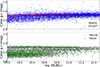 |
Fig. 1. g − r color–stellar mass diagram. Top: observational data (from MaNGA and ATLAS3D). Bottom: simulated data (from TNG50 and TNG100). Both panels encompass all samples within the mass range of 1010 − 1011.5 M⊙. Red sequence ETGs are selected above the dashed line. |
3. Sample selection and mock observations of IllustrisTNG simulation galaxies
The TNG simulations use a Lambda cold dark matter (ΛCDM) setup with the cosmological parameters from the Planck survey (Planck Collaboration I 2016), and it exploits all the advantages of the unstructured moving-mesh hydrodynamic method Arepo11 (Springel 2010) but improves the numerical methods, the subgrid physical model, and the recipe for galaxy feedback both from stars and Active Galactic Nucleus (AGNs). In particular, TNG is equipped with a novel dual mode (thermal and kinetic) AGN feedback that shapes and regulates the stellar component within massive systems, maintaining a realistic gas fraction (Weinberger et al. 2017). Also, the feedback model from galactic winds has been improved to better represent low- and intermediate-mass galaxies (Pillepich et al. 2018b).
The TNG suite comprises three runs using different simulation volumes and resolutions, namely TNG50, TNG100, and TNG300 (Nelson et al. 2018; Naiman et al. 2018; Marinacci et al. 2018; Pillepich et al. 2018a, 2019; Springel et al. 2018). Each run begins at z = 127 using the Zeldovich approximation and evolves down to z = 0. In this study, we used TNG50-1 (hereafter, simply TNG50) and TNG100-1 (hereafter, simply TNG100) runs. TNG50 provides a high number of galaxies for statistical analyses and a “zoom-in”-like resolution. TNG50 includes 2 × 21603 initial resolution elements in a ∼50 comoving Mpc box, with the baryon mass resolution of 8.5 × 10⁴ M⊙ and a gravitational softening radius rsoft for stars of about 0.3 kpc at z = 0. Dark matter (DM) was resolved with particles of mass 4.5 × 10⁵ M⊙. Meanwhile, the minimum gas softening reaches 74 comoving parsecs. TNG100 includes approximately 2 × 18203 resolution elements in a ∼110 comoving Mpc box. The DM and baryonic mass resolutions of TNG100 are mDM = 7.5 × 10⁶ M⊙ and mb = 1.4 × 10⁶ M⊙, respectively (Springel & Hernquist 2003). The softening length employed for TNG100 for both the DM and stellar components is ϵ = 0.74 kpc, while an adaptive gas gravitational softening is used, with a minimum ϵgas, min = 0.185 kpc. TNG50 thus has roughly 15 times better mass resolution, and 2.5 times better spatial resolution, than TNG100 (Nelson et al. 2019).
The identification of galaxies in the simulations was performed using the friends-of-friends (FoF) group finding algorithm (Davis et al. 1985) and the SUBFIND algorithm (Springel et al. 2001; Dolag et al. 2009). The central galaxy (subhalo) is the first (most massive) subhalo of each FoF group, while the other galaxies within the FoF group are its satellites. All components, including gas, stars, DM, and black holes, gravitationally bound to a single galaxy are associated with their host subhalo. Each galaxy was positioned at the minimum of its respective gravitational potential well. This study utilized galaxies from snapshot #99 (corresponding to z = 0) in both TNG50 and TNG100.
3.1. Sample selection of early-type galaxies
Nelson et al. (2018) showed that TNG simulations reproduce realistic galaxy colors matching SDSS observations (Strateva et al. 2001). Redder galaxies in TNG exhibit typical ETG-like properties: suppressed star formation, low gas fractions, higher metallicities, and older stellar populations. Firstly, we selected all galaxies with stellar masses within the range of 1010.0 ≤ M* ≤ 1011.5 M⊙, including both central and satellite galaxies. Then we identified ETGs using the color-mass diagram (Figure 1, lower panel), applying the same color selection criteria (dashed lines) and the same stellar mass range as for the observations. While TNG color measurements ignore dust effects, we validated our ETG selection using a deep learning classifier (Huertas-Company et al. 2019) trained on Nair & Abraham (2010) data12. This morphological analysis confirmed that 85% of color-selected TNG100 galaxies are genuine ETGs (1693 E/S0 systems), with the remaining 15% being spiral galaxies. Tests show this contamination negligibly impacts our results, justifying our color-only selection approach for TNG samples.
In addition, we excluded galaxies where the effective radius Re fell below twice the gravitational softening length (Re < 2rsoft) where rsoft is 0.74 kpc and 0.288 kpc in TNG100 and TNG50, respectively. This criterion eliminated five objects (2.0% of the TNG50 parent sample; N = 244) and 245 objects (9.4% of the TNG100 parent sample; N = 2602). We further excluded merger-contaminated galaxies through visual inspection of stellar density maps. After applying these criteria, our final ETG sample consisted of 2342 and 236 galaxies from TNG100 and TNG50, respectively.
The ATLAS3D parent sample, which includes 260 ETGs as well as 611 spiral galaxies at z ≲ 0.01, has been confirmed as a complete and representative sample of the nearby galaxy population, with an ETG fraction of approximately 30% (260/871) (Cappellari et al. 2011a). In the TNG simulations, our selection criteria yield ETG fractions of 27% (236/873) in TNG50 and 35% (2342/6369) in TNG100. By comparison, an observational sample (MaNGA) at z < 0.05 (Section 2.2) classifies 23% of galaxies as ETGs, a value closely aligned with TNG50. A separate local sample (0.05 < z < 0.1, g < 16 mag) reports a higher ETG fraction of 33% (14 034 galaxies) (Nair & Abraham 2010). TNG100 appears to reproduce a more consistent overall fraction of ETGs, while the discrepancy between TNG100 and TNG50 suggests that TNG50 may underestimate quenching efficiency. Meanwhile, in terms of spatial coverage and environmental representation, TNG50 broadly aligns with the ATLAS3D survey in sampling low-density cosmological regimes (e.g., Cappellari et al. 2011b), while TNG100 corresponds to MaNGA’s cosmological volume (z < 0.05), which incorporates higher-density environments (e.g., Goddard et al. 2017; Greene et al. 2017). Shown in Figure 2, the stellar mass distributions of TNG50 and TNG100 galaxies show no clear differences attributable to their cosmological environments. And these environmental differences between simulation pairs do not fully account for the observational-simulation discrepancies we found (see details in Section 6.3).
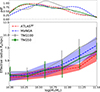 |
Fig. 2. Mass–size relation. Top: stellar mass distribution function of the chosen sample of ETGs from observational data and the TNG simulations. Bottom: Circularized effective radii Re, of the selected ETG samples in the TNG100 and TNG50 simulations as a function of stellar mass and compared with observations (ATLAS3D and MaNGA). Both TNG50 (solid green line) and TNG100 (solid gray line) galaxies share comparable stellar masses and sizes with the ATLAS3D (dashed red line) and MaNGA (dashed blue line) galaxies. The lines and points represent the median values, with colored regions and error bars indicating the 16th to 84th percentile range of each distribution. To avoid overlap, we shift the error bars slightly for clarity. |
3.2. Mock images and data extraction
3.2.1. Mass and size
We define the total stellar mass M* as the total bound stellar mass of the galaxy. That is, the calculation of the total stellar mass utilizes the complete set of particle data associated with galaxies and subhalos, encompassing all gravitationally bound particles identified through the SUBFIND algorithm. The effective radius Re is estimated by the circularized effective radius in a similar way to that of observations, where the area of the ellipse that encloses half of M* is equated to  .
.
The multi-Gaussian expansion (MGE) fitting is conducted using the Python package MGEFIT13 (Cappellari 2002) on the 2D stellar mass map within an area of 60 kpc × 60 kpc. The stellar surface density in the MGE fitting is expressed as
![Mathematical equation: $$ \begin{aligned} \Sigma (x\prime , { y}\prime ) = \sum _{k = 1}^{N} \frac{\Sigma _k}{2\pi \sigma _{k}^2 q_{k}^{\prime }} \exp \left[-\frac{1}{2 \sigma _{k}^2} \left(x{\prime }^{2} + \frac{{ y}{\prime }^{2}}{q_{k}^{\prime \,2}}\right)\right], \end{aligned} $$](/articles/aa/full_html/2026/03/aa57316-25/aa57316-25-eq8.gif) (1)
(1)
where Σk, σk, and  represent the total stellar mass, dispersion along the major axis, and axial ratio of the k-th Gaussian component, respectively. MGEFIT outputs the 2D half-mass radius Re and semimajor axis
  based on the 2D stellar mass distribution in the MGE formalism. It should be noted that the MGE approach does not extrapolate the light or density of a galaxy to infinite radii when determining Re. Beyond three times the dispersion of the largest MGE Gaussian component, the model’s flux effectively drops to zero. As a result, this method yields a slightly smaller Re compared to other techniques (de Vaucouleurs 1948; Burstein et al. 1987; de Vaucouleurs et al. 1991). The Re and
  values used in this paper are thus scaled by a factor of 1.35, as suggested by Cappellari et al. (2013b), which subtracts potential systematic errors due to different methods.
We compare the Re and M* distributions of TNG galaxies with ATLAS3D and MaNGA samples in Figure 2. The TNG galaxies (dashed profiles) agree with observed (solid profiles) Re and M* values well. Those with M* ≥ 1010.8 M⊙ may be slightly higher (∼2 kpc), but this has minimal impact on our results. Moreover, we also examined the measurement using r−band luminosity images. Our analysis reveals that Re measured by r-band fitting yields a slightly higher value by ≲1 kpc than those of mass-based measurements, propagating to a marginal increase in ΔλR(Re)≲0.03. Though quantifiable, these differences negligibly impact our kinematic conclusions.
3.2.2. Kinematic maps and their Fourier expansion models
We computed the line-of-sight (LOS) mean velocity and velocity dispersion fields for TNG galaxies from a randomly oriented perspective. All images are binned into 0.2 kpc intervals, equivalent to 2 arc seconds for a galaxy at a distance of 20 Mpc. This creates mock kinematic observations comparable to the ATLAS3D survey (Cappellari et al. 2011a). Examples of fast (left panels) and slow (right panels) rotators are shown in Figure 3. Stellar particles are grouped into a regular grid centered on the galaxy, spanning a width of 40 kpc. Voronoi binning14 (Cappellari & Copin 2003) is then applied to merge bins with an insufficient number of stellar particles. Due to the Poissonian noise in particle counts, the target S/N relates to the number of particles per bin as  . To achieve robust kinematics, we set S/N ≥ 10, requiring at least 100 stellar particles per bin. The mean velocity and velocity dispersion of the i-th bin are calculated as
 (2)
(2)
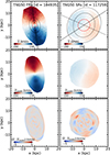 |
Fig. 3. Velocity maps and models of examples of a FR (left) and a SR (right), with raw data (top), a reconstructed velocity field employing a pure cosine law along ellipses (middle), and residuals depicting deviations (bottom). Our visualization emphasizes structural features through isodensity ellipses spaced at regular Re intervals from Re to 3Re. The major axis orientations – with solid lines representing photometrically derived morphological axes and dashed lines indicating kinematically determined axes – are both measured at Re. |
where the index n runs over the stellar particles with mass Mn, i within ith Voronoi bin, Ni is the particle number of this bin.
We further applied the KINEMETRY package for modeling the velocity maps through a truncated Fourier expansion along elliptical contours (Krajnović et al. 2006, 2008; Foster et al. 2016):
![Mathematical equation: $$ \begin{aligned} V(\psi ) = V_0 + \sum _{n = 1}^{k} \left[A_n\sin (n\psi ) + B_n\cos (n\psi )\right], \end{aligned} $$](/articles/aa/full_html/2026/03/aa57316-25/aa57316-25-eq14.gif) (3)
(3)
where ψ denotes the eccentric anomaly, V0 represents the systemic velocity, and An, Bn are the Fourier coefficients. In the case of an ideal rotating disk, symmetry requirements force all coefficients except B1 to vanish, simplifying the velocity profile to V(ψ) = V0 + B1cos(ψ). The cosine term captures the characteristic signature of regular rotation B1 = Vrot (the second row of Figure 3), where Vrot denotes the velocity amplitude, while nonzero higher-order coefficients reveal departures from axisymmetry in the velocity field (the third row of Figure 3).
4. Parameters quantifying rotation properties of galaxies
The relative importance of rotation is a key factor that determines the morphology, assembly history, and internal dynamics of galaxies. Several dimensionless parameters are commonly employed to characterize the rotational properties of galaxies, such as λR (the classical spin parameter), κrot (cylindrical rotation energy), and structural mass ratios derived from kinematic decomposition. Meanwhile, the higher-order term  from the Fourier decomposition of velocity fields, which is used to describe kinematic anomalies, has been used to classify fast and SRs in ETGs (Emsellem et al. 2004, 2011), despite lacking a well-defined physical connection to the relative importance of rotation.
  is defined as the mass-weighted average of the fifth-order kinematic Fourier coefficient
  within the effective radius Re, where Vrot represents the velocity amplitude, A5 and B5 are the fifth sine and cosine terms, respectively, in the truncated Fourier expansion for modeling the velocity field along elliptical contours (see Equation (3)). The relationships among these parameters and their consistency with observational data are not yet fully understood.
This study systematically estimates and compares these parameters through: (1) rigorous evaluation of their diagnostic capabilities, (2) quantitative analysis of their inter-parameter correlations, and (3) direct comparison with observational results. This comprehensive approach seeks to establish a universal framework for characterizing galactic rotation and classifying of slow and FRs of galaxies in both observations and simulations.
4.1. The λR − ε diagram
The spin parameter λR is a dimensionless parameter that quantifies the rotation of galaxies as defined by Emsellem et al. (2011)
 (4)
(4)
where the weighting with the flux is substituted here with a weighting with the mass contained within the ith Voronoi bin, Mi. The value Ri is the distance of the ith bin to the galaxy center. The values λR(Re) and λR(3Re) are computed by summing over all Voronoi bins within ellipses of one and three times Re, with semimajor axis  (Graham et al. 2018)15.
Galaxies with higher rotational velocities typically exhibit larger spin parameters (λR) and lower ellipticities (ε), as illustrated in the λR − ε diagrams of Figures 4 and 5 for both TNG simulations and IFS observations.
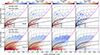 |
Fig. 4. λR(Re)−ε(3Re) diagram color-coded by κrot(all), fspheroid(all), fhalo(all), and fbulge(all) for TNG50 (upper) and TNG100 (lower). Here, κrot(all), fspheroid(all), fhalo(all), and fbulge(all) represent the significance of cylindrical rotation, the spheroidal mass fraction, the stellar halo mass fraction, and the bulge mass fraction, respectively (see Sections 4.3 and 4.4). The magenta curve shows the λR − ε relation for edge-on, axisymmetric galaxies derived by Cappellari et al. (2007). The dotted black curves illustrate this relation across varying i, with steps of Δi = 10°. Additionally, the thin dashed black lines represent the theoretical distribution for the different rotations spaced at intervals of ΔλR, intr = 0.1. The bold black curve represents our proposed new threshold for distinguishing between SRs and FRs. This threshold is derived from the tensor virial theorem for oblate galaxies with intrinsic parameters λR, intr(Re) = 0.4 and εintr = 0.525, assuming an anisotropy of δ = 0.7εintr = 0.367. For comparison, the thin solid black line represents the standard empirical threshold defined by |
Our analysis confirms a substantial galaxy population in the high-ellipticity region (ε ≳ 0.4) with intermediate-to-low λR(Re) values–occupying the right portion of the λR(Re)–ε(Re) plane. Pulsoni et al. (2020) argued that such galaxies (∼50% of total ETG samples) should be excluded as nonphysical via applying an axis-ratio cut at Re as suggested by observations (Weijmans et al. 2014; Foster et al. 2017; Li et al. 2018; Ene et al. 2018). Excluding such galaxies may induce severe selection bias. While ellipticity (ε) is commonly used to quantify inclination of galaxies, we find that these specific systems are predominantly barred galaxies, whose central ε(Re) are enhanced by the bar structure. There is no robust justification for excluding such galaxies, as the presence of elongated bar structures is unlikely to significantly alter overall galactic kinematics. To mitigate inclination errors from this central triaxiality of bars and the associated bias of excluding such galaxies, we adopted ε measured at 3Re. Seventeen of the 260 galaxies from ATLAS3D were measured at 2.5Re − 3Re, and the majority of observational data was measured at Re. This issue should not significantly affect our conclusion for fast-rotating cases. Emsellem et al. (2011) introduced an empirical threshold  (thin black curve in Figure 5) to distinguish FRs from SRs. This criterion is initially defined by the fifth-order kinematic Fourier coefficient
  , which quantifies non-axisymmetric rotational components. For instance, the bottom-right panel of Figure 3 showcases a SR with elevated
  values (see details in Section 4). This classical criterion yields about 12% SRs in TNG simulations, which is consistent with the result of both ATLAS3D and MaNGA.
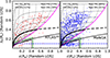 |
Fig. 5. λR(Re)−ε(Re) diagram of the ATLAS3D(left panel) and MaNGA (right panel) samples. The proportions of SRs and FRs classified using our new threshold, compared to the standard old definition, are provided at the top. The definitions of all the lines are the same as those in Figure 4. |
To assess the uncertainty in kinematic measurements at different galactocentric radii, we computed the deviation between λR values measured within Re and 3Re, as shown in Figure 6. The differences between morphologically derived position angles (PAmorph) and kinematically derived ones (PAkin) are generally minor (i.e., < 20 degrees), as PAmorph and PAphot can be derived by applying KINEMETRY to perform elliptical fitting on simulated galaxy images. In contrast, λR(Re) values are systematically lower than λR(3Re), which is expected due to the kinematic suppression often caused by central slow-rotating components such as bulges. This radial dependence highlights the importance of well-defined apertures in kinematic analyses, particularly for galaxies with structurally complex components. For consistency, we adopted 3Re measurements to represent accurate galactic properties, while Re measurements were retained for direct comparison with observational studies.
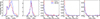 |
Fig. 6. Distributions of the differences between various galactic parameters measured within (at) 3Re and Re isodensity ellipses. From left to right: λR(3Re)−λR(Re), ε(3Re)−ε(Re), PAmorph(3Re)−PAmorph(Re), PAkin(3Re)−PAkin(Re), and i(3Re)−i(Re). Here, λR(3Re), ε(3Re), PAmorph(3Re), and PAkin(3Re), i(3Re) represent the respective parameters measured within (at) 3Re, while λR(Re), ε(Re), PAmorph(Re), PAkin(Re), i(Re) denote the same parameters but measured within (at) Re isophoto. The red and blue histograms signify the galaxies in TNG50 and TNG100, respectively. |
In addition, the inclinations for the observational data were derived from JAM modeling, which is quite time-consuming. Therefore, we used the simple correlation  that allowed us to apply our method to more IFS data where dynamical modeling was not available. We computed the deviation between i values measured within Re and 3Re, as shown in the right-most panel of Figure 6. The differences between i(3Re) and i(Re) are generally minor.
4.2. Approximation of the intrinsic spin parameter λR, intr
The location of galaxies within the λR − ε diagram is influenced not only by their rotational properties but also by their inclination angles. To correct for this projection effect, we estimated an intrinsic spin parameter, λR, intr, which approximates the spin value for an edge-on configuration (i = 90°), under the assumption that galaxies are axisymmetric systems. Following the method of Binney & Tremaine (1987), we derived the edge-on (V/σ) as
 (5)
(5)
where the observed ratio  is computed along the line of sight for a given inclination angle i. The value δ denotes the velocity anisotropy randomly sampled from a uniform distribution in the empirically motivated range [0, 0.7εintr], as suggested by Cappellari et al. (2007). We derived the edge-on ellipticity by
  . We then approximated the intrinsic spin parameter λR, intr by the empirical formula from Emsellem et al. (2007, 2011):
 (6)
(6)
where a = 1.1. λR, intr roughly corresponds to the values of λR projected onto the magenta curve in Figures 4 and 5.
To assess how accurately this method recovers λR, intr, we calculated the deviation ΔλR, intr between the intrinsic spin parameter and approximated its real values in edge-on views, specifically for the TNG galaxies, as shown in Figure 7. The distributions for TNG50 (red histograms) and TNG100 (blue histograms) reveal no significant differences in λR, intr measurements within Re (left panel) versus within 3Re (right panel). The results demonstrate that the method reliably recovers the intrinsic spin parameter, with deviations falling within acceptable limits.
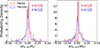 |
Fig. 7. Distribution of the deviation ΔλR, intr within different regions between the intrinsic spin parameter and its edge-on projection. Left panel: Distribution of the deviation ΔλR, intr(Re). Right panel: Distribution of the deviation ΔλR, intr(3Re). The red histogram signifies the galaxy sample derived from TNG50, whereas the blue histogram represents the galaxy sample from TNG100. The vertical dashed lines show the median of the intrinsic spin spectroscopic parameter estimation error. The median and the 16th and 84th percentiles are listed at the top right of each subplot. |
4.3. Mass fractions of kinematically derived structures using auto-GMM: spheroid fspheroid and stellar halo fhalo
Recent studies (Du et al. 2019, 2020, 2021) introduced auto-GMM, an automated unsupervised method for accurately decomposing galaxy kinematic structures in simulation data. This approach analyzes stellar particles in a 3D kinematic phase space comprising the circularity parameter ϵ = jz/jc(e) (Abadi et al. 2003), the non-azimuthal angular momentum ratio jp/jc(e), and the normalized binding energy e/|e|max (Doménech-Moral et al. 2012). The value jz denotes the specific angular momentum component aligned with the galaxy’s minor axis (z-axis) in cylindrical rotation. This quantity is normalized by jc(e), the maximum possible circular angular momentum corresponding to the particle’s binding energy e. The parameter jz/jc(e) thus quantifies rotation aligned with the galaxy’s net angular momentum, whereas jp/jc(e) measures misaligned rotation, and e/|e|max indicates how tightly bound each stellar particle is.
When applied to TNG simulations, this method successfully identified distinct structural components, including cold disk, warm disk, bulge, and stellar halo. The total spheroidal mass fraction fspheroid was obtained by combining the contributions from both the bulge (fbulge) and the stellar halo (fhalo), with data taken from Du et al. (2020) and Du et al. (2021)16. The measurements are provided at three different scales: f(Re) for stars within 1Re, f(3Re) within 3Re, and f(all) for all stars in each galaxy. fhalo defined in this way correlates closely with the strength of merger history (Du et al. 2021; Proctor et al. 2024). One of the key advantages of auto-GMM is its allowance for weakly rotating spheroids, differing from other studies (Zana et al. 2022; Cristiani et al. 2024; Liang et al. 2025), which assume zero rotation in bulges and stellar halos–a likely unrealistic assumption.
The spheroidal mass fraction fspheroid serves as a quantitative measure for determining the relative dominance of spheroidal components in galaxies. Based on this metric, we can classify galaxies with fspheroid < 0.5 as FRs, which means disk structures dominate them, while those with fspheroid > 0.5 are identified as SRs.
4.4. Assessing the significance of cylindrical rotation energy κrot
The significance of cylindrical rotation was quantified by the parameter ![Mathematical equation: $ \kappa_{\mathrm{rot}} = \frac{K_{\mathrm{rot}}}{K} = \frac{1}{K}\sum\left[\frac{1}{2}m_{i}\left(\frac{j_{z,i}}{R_{i}}\right)^2\right] $](/articles/aa/full_html/2026/03/aa57316-25/aa57316-25-eq30.gif) , as defined in (Sales et al. 2010), where K and m represent the total kinetic energy and mass of each stellar particle, respectively. This widely used metric provides a clear physical interpretation of ordered rotation in simulated galaxies and is computationally straightforward to evaluate.
, as defined in (Sales et al. 2010), where K and m represent the total kinetic energy and mass of each stellar particle, respectively. This widely used metric provides a clear physical interpretation of ordered rotation in simulated galaxies and is computationally straightforward to evaluate.
However, several important considerations should be noted. First, while commonly adopted, the threshold of κrot = 0.5 for distinguishing between disk galaxies (corresponding to FRs) and elliptical galaxies (SRs) lacks strong theoretical justification (Zhao et al. 2020; Roshan et al. 2021; Lu et al. 2025). Second, for a completely dispersion-dominated system, theoretical considerations predict κrot = 1/3. Finally, the physical interpretation remains ambiguous for both disk-dominated galaxies (κrot > 0.5) and elliptical galaxies (κrot < 0.5). These limitations highlight the need for careful interpretation when applying κrot criteria to different galactic systems.
5. Approximating κrot and fspheroid from scaling relations with λR, intr
The intrinsic spin parameter λR, intr, together with the λ − ε diagram, offers a relatively accessible observational metric. A higher λR, intr value signifies that a galaxy’s kinematic structure is dominated by ordered rotation, while a lower value indicates a greater influence of random motion. Consequently, Figure 4 reveals a clear trend: both fspheroid and κrot decrease as λR, intr declines. In this section, we quantitatively examine the scaling relations connecting λR, intr, κrot, and fspheroid.
We begin by investigating the relationship between λR, intr and κrot. The fundamental difference in their velocity dependence – linear for λR, intr versus quadratic for κrot – motivates a quadratic fitting function of the form:
 (7)
(7)
where A, B, and C represent the coefficients to be determined through regression analysis. This functional form naturally accommodates their distinct velocity scalings while enabling quantitative comparisons of their kinematic relationship. The first row of Figure 8 reveals a robust correlation between λR, intr and κrot (see the fitting result at the bottom-right corners). This relationship holds consistently across both TNG50 (red) and TNG100 (blue) simulations, regardless of the measurement aperture - whether considering stars within Re, 3Re, or the entire system. Notably, as demonstrated in the right-most panel, λR, intr(Re) alone can be used to approximate the global κrot(all) with an acceptable uncertainty of ∼0.05, despite being measured only within the effective radius (Re). Furthermore, the criterion κrot > 0.5 has become a standard threshold for identifying disk-dominated systems in numerical simulations, approximately equivalent to λR, intr(Re)≳0.4.
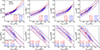 |
Fig. 8. Distribution and correlation of κrot vs. λR, intr (upper) and fspheroid vs. λR, intr (lower) measured within different regions from left to right. The solid red and blue curves show the best-fit results for the TNG50 and TNG100 datasets, respectively, while the dashed curves represent their 2σ confidence interval. The corresponding fitting coefficients and σ values are listed in the bottom-right corner of each panel. In the lower panels, we additionally provide the Pearson correlation coefficient (rp). The rp ∼ −1 value indicates a strong anticorrelation between λR, intr and fspheroid. |
Our analysis further reveals a linear scaling relation between λR, intr and fspheroid, as shown in the lower panels of Figure 8. This correlation robustly validates λR, intr as an effective diagnostic for quantifying spheroid mass fractions across different measurement apertures; see the fitting result at the bottom-right corners. The observed anticorrelation follows fspheroid ≈ 1 − λR, intr (or equivalently, fdisk ≈ λR, intr), indicating that λR, intr directly traces disk dominance with a typical uncertainty of σ ∼ 0.1. This establishes λR, intr as a powerful observational proxy for connecting IFS kinematics to the intrinsic structural decomposition of galaxies. Even when limited to one effective radius (λR, intr(Re)) – the typical spatial coverage of IFS observations – λR, intr retains diagnostic power for characterizing global galaxy rotation.
The parameter λR thus can serve as a proxy for estimating λR, intr, κrot, and fspheroid. Empirically, λR, intr(Re) provides a reasonable approximation of the global rotational properties, specifically κrot(all) and fspheroid(all). Moreover, it is worth highlighting that the λR, intr − fspheroids relationship is primarily determined by fhalo, shown in the third column of Figure 4. Bulges only contribute to scatter without altering the fundamental scaling relation, as shown in the fourth column. In the fourth column, we further leverage the empirical correlations between λR, intr(Re) and κrot(all), fspheroid(all) derived from TNG50 simulations to infer approximate values of κrot(all) and fspheroid(all) based on λR, intr(Re)17 for observed galaxies. Details on a subset of MaNGA galaxies, specifically nine randomly selected sample galaxies, are listed in Table 1. The complete content of MaNGA, ATLAS3D, TNG50, and TNG100 data is publicly available.
Main properties of the 933 MaNGA galaxies used in this paper.
6. Kinematic classification of galaxies into fast (disk) and slow (elliptical) rotating galaxies
In this study, we equate disk galaxies with FRs and elliptical galaxies with SRs. Regarding this, it should be noted that morphological classifications (disk vs. elliptical galaxies) and kinematic classifications (FRs vs. SRs) describe fundamentally distinct galaxy properties. Disks and ellipticals denote visual structures observed photometrically (e.g., spiral arms vs. smooth ellipsoids; Hubble 1926, 1936; Sandage 2005), while FRs and SRs categorize galaxies based on dynamical properties quantified by spin parameter λR (Emsellem et al. 2007; Cappellari 2016). Historically, these classifications strongly correlated–ellipticals were presumed pressure-supported SRs, while disks were rotationally dominated FRs–driving early unification in literature. However, IFS surveys such as ATLAS3D, SAMI, CALIFA, and MaNGA have revealed significant exceptions: part of morphological ellipticals exhibit FR kinematics (Emsellem et al. 2011; Fogarty et al. 2015), and a minority of disks show SR-like suppression of rotation (Falcón-Barroso et al. 2015; Graham et al. 2018). Thus, equating disks and ellipticals directly with FRs and SRs overlooks dynamically complex populations and risks oversimplification.
Therefore, this work introduces unified classification thresholds that reconcile galaxy morphology and kinematics (see Section 6.2). Our criteria reclassify approximately 4% of previously identified disk galaxies as ellipticals and approximately 16% of FRs as SRs. With the associated publicly released catalog (Table 1), we establish a consistent disk and FR as well as elliptical and SR mapping applicable to both observational surveys and cosmological simulations.
6.1. Failure of the empirical classification of slow/fast rotators: The high-order Fourier kinematic components  and the empirical λR(Re)−ε criterion
To evaluate the reliability of the standard FRs and SRs classification in previous studies (e.g., Krajnović et al. 2011; Emsellem et al. 2011), we also calculated the  (see Section 4). However, we find that
  exhibits no significant correlation with either κrot or fspheroid, suggesting it poorly traces kinematic disk structure or global rotation (Figure 9), where it is assumed that galaxies with fspheroid < 0.5 or κrot > 0.5 are classified as FRs (disk-dominated), while those with fspheroid > 0.5 or κrot < 0.5 are classified as SRs (spheroid-dominated). This implies that both
  and the standard λR − ε criterion (thin black profiles in Figures 4 and 5) inadequately distinguish SRs from FRs, though they successfully identify extreme slow-rotating cases (Lu et al. 2023).
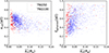 |
Fig. 9. κrot(all), fspheroid(all) of the selected ETGs samples in TNG simulation, plotted as a function of |

Moreover, SRs are typically identified using other empirically derived thresholds in the λR(Re)−ε plane. Common selection criteria include: 1) Emsellem et al. (2007)’s constant threshold λR(Re) < 0.1 (dashed blue line in Figure 4); (2) Emsellem et al. (2011)’s scaling relation  (black curve); 3) Cappellari (2016)’s polygon criterion requiring λR(Re) < 0.08 + ε/4 with ε < 0.4 (black polygon); and 4) van de Sande et al. (2021)’s adaptable threshold λR(Re) < λRstart + ε/4 where ε < 0.35 + λRstart/1.538 (green polygon), adopting λRstart = 0.12 for SAMI-like data quality. Given the functional similarity of these thresholds–particularly their convergence near
  –we designate the Emsellem et al. (2011) relation as our reference criterion for distinguishing classical FRs from SRs. A revised threshold, better quantifying galactic rotation, is needed to reliably classify SRs in observations and enable robust comparisons with simulations.
6.2. Reclassification of fast and slow rotators through the kinematic bimodality
As established in the Section 5, λR, intr exhibits strong correlations with both fspheroid and κrot, confirming its utility as a fundamental parameter for characterizing galactic rotation and classifying slow versus FRs.
Figure 10 shows a pronounced bimodality in kinematic properties, with well-separated peaks for fast and SRs. Both the ATLAS3D and MaNGA surveys exhibit this dichotomy:
-
Fast rotators (FRs) / disk galaxies are characterized by high intrinsic spin (λR, intr(Re)∼0.7), thus strong rotational support (κrot ∼ 0.7) and low spheroid fractions (fspheroid ∼ 0.3).
-
Slow rotators (SRs) / elliptical galaxies have low spin (λR, intr(Re)∼0.2), weak rotation (κrot ∼ 0.3), and dominant spheroid components (fspheroid ∼ 0.8).
The vertical dashed black lines in Figure 10 mark the new thresholds we suggest for distinguishing slow and FRs, giving λR, intr ∼0.4, κrot ∼ 0.5, and fspheroid ∼ 0.6. These thresholds roughly correspond to the minimum probability of the bimodal distributions. The threshold λR, intr ∼0.4 is exactly same to that suggested by Wang et al. (2024). This bimodal distribution persists across all mass ranges, revealing a significant population of rapidly rotating ETGs. Notably, the κrot ∼ 0.5 threshold – commonly used in simulations to select disk galaxies – proves observationally robust for identifying FRs and disk galaxies. We maintain the conventional designations of SRs and FRs but introduce refined kinematic thresholds to better distinguish between these populations. This update ensures consistency with established nomenclature while improving the physical accuracy of the classification scheme.
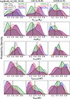 |
Fig. 10. Probability density distributions of λR, intr(Re), λR(Re), κrot(all), fspheroid(all), and fhalo(all). The solid green, solid gray, dashed blue, and dashed red profiles represent ETG samples of TNG50, TNG100, MaNGA, and ATLAS3D, respectively. From left to right: Three stellar mass ranges of 1010 − 1010.4 M⊙, 1010.4 − 1010.8 M⊙, and 1010.8 − 1011.5 M⊙. In the top right corner of each upper panel, we give the proportion and absolute count of galaxies within each mass range relative to the total ETG sample. From top to bottom, these vertical dashed black lines represent λR, intr(Re) = 0.4, λR(Re) = 0.3, κrot(all) = 0.5, fspheroid(all) = 0.6, and |

The distribution of spin parameter (λR) is shown in the second row of Figure 10. As λR constitutes the projected counterpart of intrinsic λR, intr, it follows that λR ∼ λR, intr sin i when assuming the galaxy as an isotropic thin disk (see Equation (6)). This systematic projection effect depresses observed λR values below their intrinsic values. For FRs, the peak shifts from an intrinsic value of λR, intr ∼ 0.65 to a lower observed value near λR ∼ 0.55. The threshold decreases to 0.3. It further weakens the bimodality in the distribution and reduces the diagnostic power of λR alone, making it less accurate than λR, intr for distinguishing between fast and SRs. Furthermore, van de Sande et al. (2021) selected ETGs in the SAMI Galaxy Survey using visual morphology, reporting a similarly bimodal distribution of λRe values. As shown in their Figure 8, these bimodality peaks occur near λR(Re)∼0.5 and λR(Re)∼0.1 within a comparable stellar mass range to our sample – a result consistent with our findings from both MaNGA and ATLAS3D.
Figure 10 clearly shows a distinct population divergence between FRs classified according to our new threshold (thick solid black profiles in Figure 4) and those identified using the conventional criterion (thin solid black profiles in Figure 4). Under the previous classification scheme, only galaxies with minimal disk components and weak rotational support–specifically elliptical systems meeting the conditions κrot < 0.4, fspheroid > 0.8, and fhalo > 0.6 – were categorized as SRs. The TNG simulations exhibit approximately 10% more SRs compared to observational samples. Nevertheless, the overall fraction of SRs in TNG remains consistent with those derived from both the ATLAS3D and MaNGA surveys. Moreover, the proposed threshold offers a universal criterion for classifying galaxies of all types – including both early-type and late-type galaxies – based on their rotational properties.
6.3. Kinematic bimodality deficiency in TNG: Systematic under-rotation of simulated ETGs
While the TNG simulations reproduce a similar overall proportion of SRs to observations – as detailed in Section 6.2 – they exhibit a less distinct kinematic bimodality. This discrepancy arises from an overabundance of galaxies with intermediate rotational support, as shown in Figure 10. Both TNG50 and TNG100 show a significant deficit of FRs, leading to a systematic shift toward lower intrinsic spin parameter (λR, intr) values throughout the simulated population. This deficiency of fast-rotating ETGs in TNG simulations results in systematically different kinematic properties compared to observations: simulated ETGs exhibit weaker rotation (lower κrot), higher spheroid fractions (fspheroid), and higher stellar halo fractions (fhalo), as shown in Figure 10. This result manifests two primary shortcomings: (1) a near-total absence of rapidly rotating systems with λR, intr > 0.6, and (2) a displacement of the characteristic λR, intr peak from the observed value of ∼0.7 to below 0.5. Correspondingly, the simulations contain an overabundance of slow-rotating ETGs and yield a higher fraction of ETGs with significant spheroidal components (fspheroid > 0.5), many of which represent disk galaxies embedded within massive stellar halos (He et al. 2025).
It is worth highlighting that the ATLAS3D survey contains approximately 16% fewer massive galaxies compared to MaNGA (27% vs. 43%), as evidenced by the sparse population in the top-right corner of Figure 10 and the stellar mass distribution shown in Figure 2 (top panels). This disparity likely reflects MaNGA’s selection bias toward more massive systems, but this issue has no clear effect on the kinematic bimodality, as shown in Figure 10. TNG100 and TNG50 reproduces the ATLAS3D mass distribution reasonably well, though TNG100 slightly overproduces galaxies in the 1010.4 − 1010.8 M⊙ range and underrepresents the less massive ETGs. The less pronounced kinematic bimodality is thus unlikely to be caused by the discrepancy of the proportion of ETGs within each mass range relative to the total ETG sample.
This systematic discrepancy suggests that TNG simulations produce galaxies with higher spheroid and stellar halo mass fractions than those observed. It is still unclear what reasons cause this difference. It may stem from an insufficient numerical resolution to accurately capture structural properties and their dynamical evolution, particularly in central regions, such as bars, gas inflows, and other nuclear fast-rotating structures. Furthermore, the treatment approaches of the interstellar medium and feedback subgrid models also have an impact on the kinematics in especially the inner regions of galaxies. Active galactic nuclei and stellar feedback shape the star formation history and even kinematic features via regulating gas cooling and quenching (Weinberger et al. 2018; Donnari et al. 2021). Although TNG simulations successfully reproduce many galactic properties, accurately matching observed kinematic distributions remains challenging. It is also important to note that observational IFU measurements are typically limited to central regions (within approximately Re), which cannot fully represent the overall rotational characteristics of galaxies and introduce significant uncertainties. Consequently, the apparent bimodality observed in kinematic distributions may also be subject to reliability concerns. Moreover, as mentioned in Section 3.1, TNG50 appears to produce a smaller proportion of ETGs (27%) compared to observations (33%). This result also indicates that disk galaxies in TNG simulations exhibit lower quenching probabilities into early-type morphologies compared to observations. Consequently, in the real universe, systems with significant disk components appear more susceptible to quenching processes that transform them into ETGs–a transition that current simulations may not fully capture.
6.4. A novel method for approximating stellar halo mass fractions using λR, intr
The ubiquitous presence of massive stellar halos fundamentally challenges conventional galaxy classification and structural decomposition methods (Gadotti & Sánchez-Janssen 2012; Du et al. 2020; He et al. 2025). These halos primarily form through merger-driven processes – particularly major mergers and strong tidal interactions – which efficiently disrupt the disks of both progenitor and satellite galaxies (Du et al. 2021). In halo-embedded disk systems, also called Sombrero-like galaxies, where low-mass disks are embedded within massive stellar halos, traditional morphological analyses often misclassify halo mass as part of the disk structure (Du et al. 2020; He et al. 2025), leading to systematic underestimation. While classical bulges have served as historical proxies for merger activity (e.g., Toomre 1977; Aguerri et al. 2001), TNG simulations demonstrate their inadequacy in capturing the full scope of merger histories (Du et al. 2021), necessitating more robust diagnostics.
Stellar halos and suppressed rotation serve as sensitive tracers of galactic merger events, as mergers dynamically convert ordered rotation into random motion, although some disk will survive from mergers with special orbital configuration (Zeng et al. 2021). This process simultaneously builds up stellar halos and erases disk kinematics. The first row of Figure 11 reveals a moderate anticorrelation between λR, intr and the stellar halo fraction fhalo derived from auto-GMM analysis, though with a substantial scatter of σ ∼ 0.15.
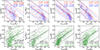 |
Fig. 11. Correlations of λR, intr versus fhalo and f′halo versus fhalo. Top row: Relationships between λR, intr and fhalo measured within Re (first column), 3Re (second column), and for all stars (third column). Fourth column: Relation between λR, intr(Re) and fhalo(all). The solid red and blue lines, along with their corresponding dashed lines, represent the linear fits and 2σ confidence interval for the TNG50 and TNG100 datasets, respectively. Fit coefficients, σ values, and Pearson correlation coefficients (rp) are provided in the top-right corner of each panel. Second row: Similar layout, but illustrating the relationship between f′halo and fhalo. Here, the solid black and green lines, with accompanying dashed lines, indicate the linear fits and 2σ confidence interval for the TNG50 and TNG100 datasets, respectively. |
We therefore introduce a novel methodology that leverages the λR, intr–fspheroids relation established in Section 5 to estimate stellar halo masses, despite the considerable associated uncertainty. Our approach computes f′halo = fspheroids − f′bulge, where bulges are operationally defined as bright central concentrations according to classical morphological criteria (Hubble 1936; Buta 2013), without distinguishing between classical and pseudo-bulge subtypes. The bulge mass fraction f′bulge is approximated by integrating the stellar surface density profile over the central 0–1 kpc region in face-on projections, while fspheroids is approximated using the scaling relation with λR, intr. Meanwhile, we examine whether f′bulge deviates further from fbulge if f′bulge is approximated by integrating the stellar surface density profile within the central 0–2 kpc or 0–3 kpc regions.
We anticipate improved accuracy with future IFS measurements extending to larger radii, as suggested by the second and third columns of Figure 11. It is noteworthy that currently, tracer populations such as planetary nebulae can, to a certain extent, already facilitate the extension of IFS measurements to larger radii (e.g., Pulsoni et al. 2018). For f′halo we obtain a somewhat acceptable agreement with dynamically derived fhalo values, exhibiting a scatter of approximately σ ∼ 0.15. It is worth mentioning that this method is unable to measure stellar halos with f′halo ≲ 0.3, where the stellar halo is too small. This method enables a somewhat statistical analysis of ETG merger histories with massive stellar halos using IFS measurements (e.g., Huang et al. 2013; Deason et al. 2016; D’Souza & Bell 2018; Monachesi et al. 2019; Du et al. 2021; Zhu et al. 2022), overcoming limitations inherent in purely morphological stellar halo identification.
7. Radial distribution of Vrot/σ in the inner regions of selected fast rotators
Fast-rotating ETGs, characterized by λR, intr > 0.4 as defined in Section 6.2, serve as ideal tracers of minimally disturbed galactic evolution (van Dokkum et al. 2015; Cappellari 2016; Wang et al. 2020; Zhu et al. 2024). Their kinematic radial profiles, relatively unaffected by major mergers or strong tidal interactions, provide critical benchmarks for studying intrinsic galaxy evolution in both simulations and observations. We thus compare the radial distribution of Vrot/σ in Figure 12. To systematically account for the effects of stellar mass and inclination, we categorize our galaxy sample into three mass bins from left to right. Each mass bin is further divided into two inclination subgroups, i.e., i = 30° −60° and i = 60° −90°, from top to bottom. This comprehensive sampling strategy enables us to isolate fundamental kinematic trends while controlling for projection effects and mass-dependent behaviors.
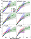 |
Fig. 12. Median Vrot/σ profiles for FRs selected using our new threshold (κrot(all) > 0.5), projected along a random LOS. Top row: Galaxy samples that fall within mass ranges [1010.0, 1010.4] M⊙, with galaxy samples presented at different inclinations: 30° −60° and 60° −90°, respectively, from left to right. The solid green lines, solid gray lines, dashed red lines, and dashed blue lines, along with their corresponding shaded regions in the figure, represent the data from TNG50, TNG100, ATLAS3D, and MaNGA, respectively. The datasets from the simulation and the observation showcase median profiles, with shaded regions indicating the 16th and 84th percentiles of the distribution. Vertical and horizontal dashed lines are included as visual aids for comparing simulations and observations. The profiles of the simulated ETG FRs closely resemble those observed. Middle and bottom rows: same as the top row, but with galaxy samples that fall within mass ranges [1010.4, 1010.8] M⊙ and [1010.8, 1011.5] M⊙. |
We utilized KINEMETRY to separately fit the galaxy’s velocity field V and velocity dispersion field σ, to obtain the radial distributions of Vrot and σ for each galaxy. Figure 12 shows that the kinematic properties of fast-rotating galaxies in TNG50 (green) match reasonably well with ATLAS3D galaxies. TNG100 galaxies exhibit slightly smaller Vrot/σ values in their central regions, likely due to enhanced numerical heating effects stemming from insufficient resolution, particularly in lower-mass systems. The MaNGA survey similarly shows somewhat depressed Vrot/σ ratios compared to ATLAS3D, consistent with expectations given its poorer spatial resolution. In particular, the observed sharp rise in Vrot/σ within the central regions (R < 0.5Re) of some massive ATLAS3D galaxies (bottom-left panel) results from fast-rotating structures. Moreover, it is worth highlighting that Vrot/σ keeps rising toward R > Re, IFS kinematic measurements in R < Re clearly cannot characterize the full dynamical state of FRs. The potential existence of massive stellar halos around disks (Gadotti & Sánchez-Janssen 2012; He et al. 2025), for example the Sombrero galaxy, may significantly change the overall λR and Vrot/σ at large radius.
Our results indicate that the TNG simulations produce a substantially larger population of galaxies with intermediate rotational support, as detailed in Section 6.2. Although TNG50 reproduces the kinematic properties of fast-rotating ETGs – consistent with previous studies (Xu et al. 2019; Zhang et al. 2025) – it is important to note that those earlier studies did not exclude the potential effect of SRs in their samples, a methodological choice that may obscure kinematic distinctions via inducing large scatters. It may diminish the visibility of potential discrepancies. Furthermore, differences in the inclination angles among galaxy samples can also influence the analysis. This overabundance of intermediate-rotators in TNG could explain the shallower Vrot/σ(R) radial profiles reported in Pulsoni et al. (2020).
8. Discussions: evaluating kinematic analysis in advanced cosmological simulations
Similar analyses have suggested consistency between TNG simulations and observations. However, when incorporating careful prevalence estimates and inclination corrections, certain discrepancies emerge. The random orientation of galaxies may introduce nonnegligible scatter in λR − ε diagrams, potentially accentuating apparent simulation-observation agreement – as exemplified by the close but uncorrected alignment shown in Figures 4 and 5. The differences in probability density profiles are discernible (Figure 10, second row). A typical inclination angle i varies between 30 and 60 degrees, which reduces the spin parameter we measured along the line of sight by a factor of sin(i)≈0.5 − 0.8. The λR values of FRs, generally within the range of 0.3–0.7, can thus be significantly underestimated. This geometric effect further reduces the potential kinematic discrepancies between observations and simulations. The λR − ε diagram thus alone cannot conclusively establish kinematic consistency between datasets.
Our results highlight the importance of refined analyses when evaluating simulation-observation consistency for not only TNG simulations. Using the Magneticum Pathfinder simulation, Schulze et al. (2018) reported general agreement in λR(Re)−ε distributions between simulated and observed ETGs. Schulze et al. (2020) further extended this approach to ∼500 galaxies (2 × 10¹⁰ M⊙ < M* < 1.7 × 10¹² M⊙), noting reasonable matches in two-point gradient relationships. Similar concordance was observed in EAGLE simulations by Walo-Martín et al. (2020) and van de Sande et al. (2019) (M > 5 × 10⁹ M⊙, z = 0), though the latter study noted systematically lower values in Horizon-AGN and Magneticum. Our findings suggest that such comparisons may benefit from explicit treatment of projection effects to ensure conclusive interpretations.
Kinematic properties serve as a fossil record of a galaxy’s formation history. Consequently, a first-order consistency between simulations and observations may be insufficient; moreover, the nonnegligible mixture of SRs and FRs in the previous classification schemes is also likely to mitigate potential discrepancy. In this study, we thus performed detailed statistical comparisons of their projection-corrected distributions across different mass ranges within a unified quantitative framework of both simulations and observations.
9. Summary and conclusions
This study presents a comparative analysis of galaxy kinematics between the TNG simulations (TNG50 and TNG100) and observational data from the MaNGA and ATLAS3D surveys. We revisited the classification of ETGs into FRs (disk-dominated systems) and SRs (dispersion-supported ellipticals) using intrinsic dynamical parameters – including the intrinsic spin parameter λR, intr, rotational energy fraction κrot, and spheroid mass fraction fspheroid. Our results show that widely adopted criteria, such as the empirical  relation and the Fourier harmonic coefficient
  , are inadequate for robust FR and SR separation due to their weak correlation with fundamental dynamical properties. We instead proposed revised thresholds (λR, intr ∼0.4, κrot ∼ 0.5, fspheroid ∼ 0.6) derived from bimodal kinematic distributions, offering a physically motivated universal distinction between rotation- and dispersion-dominated galaxies.
We also examined inter-parameter correlations among commonly used kinematic quantities and applied scaling relations derived from TNG simulations to estimate λR, intr, κrot, and fspheroid in observed MaNGA and ATLAS3D galaxies. Furthermore, we introduced a novel method for inferring stellar halo mass fractions from integral-field spectra (IFS) kinematic measurements, though current estimates remain subject to significant uncertainties.
Our comparison reveals a notable deficiency in the TNG simulations: they exhibit less distinct kinematic bimodality than observations, producing fewer FRs and showing systematically lower λR, intr values. An overabundance of galaxies with intermediate rotational support and elevated spheroid or halo fractions drives this discrepancy. Although the global fractions of SRs and FRs are roughly consistent between simulations (∼38% SRs) and observations (∼30%), the weakened bimodality in TNG reflects a failure to fully capture the dynamical diversity of real ETGs. These findings highlight the need for improved numerical resolution and more sophisticated subgrid physics in future simulations, as well as more extensive observational constraints, to advance our understanding of galaxy formation and evolution.
Data availability
Table 1 is only available at the CDS via https://cdsarc.cds.unistra.fr/viz-bin/cat/J/A+A/707/A137
Acknowledgments
The authors gratefully acknowledge insightful discussions with Luis C. Ho, Lars Hernquist, Bitao Wang, and Ling Zhu, and also extend our heartfelt gratitude to the referee for their insightful comments, which have significantly improved the quality of the paper. This work is supported by the National Natural Science Foundation of China under grant No. 12573010, the National Key R&D Program of China (No. XY-2025-1459), the Fundamental Research Funds for the Central Universities (No. 20720230015), the Science Fund for Creative Research Groups of the National Natural Science Foundation of China (No. 12221003), and the China Manned Space Program (No. CMS-CSST-2025-A10). The TNG50/TNG100 simulation used in this work, one of the flagship runs of the IllustrisTNG project, has been run on the HazelHen Cray XC40-system at the High Performance Computing Center Stuttgart as part of project GCS-ILLU of the Gauss Centers for Supercomputing (GCS). This work is also strongly supported by the Computing Center in Xi’an, China. The authors also acknowledge the assistance of DeepSeek’s AI language model in improving the language and clarity of this manuscript.
References
- Abadi, M. G., Navarro, J. F., Steinmetz, M., & Eke, V. R. 2003, ApJ, 597, 21 [NASA ADS] [CrossRef] [Google Scholar]
- Abdurro’uf, Accetta, K., Aerts, C., et al. 2022, ApJS, 259, 35 [NASA ADS] [CrossRef] [Google Scholar]
- Aguerri, J. A. L., Balcells, M., & Peletier, R. F. 2001, A&A, 367, 428 [NASA ADS] [CrossRef] [EDP Sciences] [Google Scholar]
- Arnold, J. A., Romanowsky, A. J., Brodie, J. P., et al. 2014, ApJ, 791, 80 [Google Scholar]
- Bacon, R., Copin, Y., Monnet, G., et al. 2001, MNRAS, 326, 23 [Google Scholar]
- Belfiore, F., Westfall, K. B., Schaefer, A., et al. 2019, AJ, 158, 160 [CrossRef] [Google Scholar]
- Binney, J., & Tremaine, S. 1987, Galactic Dynamics (Princeton: Princeton University Press) [Google Scholar]
- Blanton, M. R., Bershady, M. A., Abolfathi, B., et al. 2017, AJ, 154, 28 [Google Scholar]
- Blanton, M. R., & Roweis, S. 2007, AJ, 133, 734 [NASA ADS] [CrossRef] [Google Scholar]
- Blanton, M. R., Kazin, E., Muna, D., Weaver, B. A., & Price-Whelan, A. 2011, AJ, 142, 31 [NASA ADS] [CrossRef] [Google Scholar]
- Bryant, J. J., Owers, M. S., Robotham, A. S. G., et al. 2015, MNRAS, 447, 2857 [Google Scholar]
- Bundy, K., Bershady, M. A., Law, D. R., et al. 2015, ApJ, 798, 7 [Google Scholar]
- Burstein, D., Davies, R. L., Dressler, A., et al. 1987, ApJS, 64, 601 [Google Scholar]
- Buta, R. J. 2013, Secular Evolution of Galaxies (Cambridge: Cambridge University Press), 155 [Google Scholar]
- Cappellari, M. 2002, MNRAS, 333, 400 [NASA ADS] [CrossRef] [Google Scholar]
- Cappellari, M. 2013, ApJ, 778, L2 [NASA ADS] [CrossRef] [Google Scholar]
- Cappellari, M. 2016, ARA&A, 54, 597 [Google Scholar]
- Cappellari, M., & Copin, Y. 2003, MNRAS, 342, 345 [Google Scholar]
- Cappellari, M., & Emsellem, E. 2004, PASP, 116, 138 [Google Scholar]
- Cappellari, M., Emsellem, E., Bacon, R., et al. 2007, MNRAS, 379, 418 [Google Scholar]
- Cappellari, M., Emsellem, E., Krajnović, D., et al. 2011a, MNRAS, 413, 813 [Google Scholar]
- Cappellari, M., Emsellem, E., Krajnović, D., et al. 2011b, MNRAS, 416, 1680 [Google Scholar]
- Cappellari, M., McDermid, R. M., Alatalo, K., et al. 2013a, MNRAS, 432, 1862 [NASA ADS] [CrossRef] [Google Scholar]
- Cappellari, M., Scott, N., Alatalo, K., et al. 2013b, MNRAS, 432, 1709 [Google Scholar]
- Chabrier, G. 2003, PASP, 115, 763 [Google Scholar]
- Cleveland, W. S., & Devlin, S. J. 1988, J. Am. Stat. Assoc., 83, 596 [CrossRef] [Google Scholar]
- Crain, R. A., Schaye, J., Bower, R. G., et al. 2015, MNRAS, 450, 1937 [NASA ADS] [CrossRef] [Google Scholar]
- Cristiani, V. A., Abadi, M. G., Taverna, A., et al. 2024, A&A, 692, A63 [NASA ADS] [CrossRef] [EDP Sciences] [Google Scholar]
- Croom, S. M., Lawrence, J. S., Bland-Hawthorn, J., et al. 2012, MNRAS, 421, 872 [NASA ADS] [Google Scholar]
- Davé, R., Anglés-Alcázar, D., Narayanan, D., et al. 2019, MNRAS, 486, 2827 [Google Scholar]
- Davis, M., Efstathiou, G., Frenk, C. S., & White, S. D. M. 1985, ApJ, 292, 371 [Google Scholar]
- de Vaucouleurs, G. 1948, Ann. d’Astrophys., 11, 247 [Google Scholar]
- de Vaucouleurs, G., de Vaucouleurs, A., Corwin, Jr., H. G., et al. 1991, Third Reference Catalogue of Bright Galaxies [Google Scholar]
- de Zeeuw, P. T., Bureau, M., Emsellem, E., et al. 2002, MNRAS, 329, 513 [Google Scholar]
- Deason, A. J., Mao, Y.-Y., & Wechsler, R. H. 2016, ApJ, 821, 5 [NASA ADS] [CrossRef] [Google Scholar]
- Dolag, K., Borgani, S., Murante, G., & Springel, V. 2009, MNRAS, 399, 497 [Google Scholar]
- Dolag, K., Remus, R. S., Valenzuela, L. M., et al. 2025, ArXiv e-prints [arXiv:2504.01061] [Google Scholar]
- Doménech-Moral, M., Martínez-Serrano, F. J., Domínguez-Tenreiro, R., & Serna, A. 2012, MNRAS, 421, 2510 [CrossRef] [Google Scholar]
- Domínguez Sánchez, H., Margalef, B., Bernardi, M., & Huertas-Company, M. 2022, MNRAS, 509, 4024 [Google Scholar]
- Donnari, M., Pillepich, A., Joshi, G. D., et al. 2021, MNRAS, 500, 4004 [Google Scholar]
- D’Souza, R., & Bell, E. F. 2018, MNRAS, 474, 5300 [CrossRef] [Google Scholar]
- Du, M., Ho, L. C., Zhao, D., et al. 2019, ApJ, 884, 129 [NASA ADS] [CrossRef] [Google Scholar]
- Du, M., Ho, L. C., Debattista, V. P., et al. 2020, ApJ, 895, 139 [CrossRef] [Google Scholar]
- Du, M., Ho, L. C., Debattista, V. P., et al. 2021, ApJ, 919, 135 [NASA ADS] [CrossRef] [Google Scholar]
- Du, M., Ho, L. C., Yu, H.-R., & Debattista, V. P. 2022, ApJ, 937, L18 [NASA ADS] [CrossRef] [Google Scholar]
- Du, M., Ma, H.-C., Zhong, W.-Y., et al. 2024, A&A, 686, A168 [NASA ADS] [CrossRef] [EDP Sciences] [Google Scholar]
- Dubois, Y., Pichon, C., Welker, C., et al. 2014, MNRAS, 444, 1453 [Google Scholar]
- Dubois, Y., Peirani, S., Pichon, C., et al. 2016, MNRAS, 463, 3948 [Google Scholar]
- Dubois, Y., Beckmann, R., Bournaud, F., et al. 2021, A&A, 651, A109 [NASA ADS] [CrossRef] [EDP Sciences] [Google Scholar]
- Emsellem, E., Cappellari, M., Peletier, R. F., et al. 2004, MNRAS, 352, 721 [Google Scholar]
- Emsellem, E., Cappellari, M., Krajnović, D., et al. 2007, MNRAS, 379, 401 [Google Scholar]
- Emsellem, E., Cappellari, M., Krajnović, D., et al. 2011, MNRAS, 414, 888 [Google Scholar]
- Ene, I., Ma, C.-P., Veale, M., et al. 2018, MNRAS, 479, 2810 [Google Scholar]
- Falcón-Barroso, J., Lyubenova, M., & van de Ven, G. 2015, IAU Symp., 311, 78 [Google Scholar]
- Falcón-Barroso, J., Sánchez-Blázquez, P., Vazdekis, A., et al. 2011, A&A, 532, A95 [Google Scholar]
- Fall, S. M., & Rodriguez-Gomez, V. 2023, ApJ, 949, L14 [NASA ADS] [CrossRef] [Google Scholar]
- Fogarty, L. M. R., Scott, N., Owers, M. S., et al. 2015, MNRAS, 454, 2050 [NASA ADS] [CrossRef] [Google Scholar]
- Forbes, D. A., Sinpetru, L., Savorgnan, G., et al. 2017, MNRAS, 464, 4611 [Google Scholar]
- Foster, C., Pastorello, N., Roediger, J., et al. 2016, MNRAS, 457, 147 [Google Scholar]
- Foster, C., van de Sande, J., D’Eugenio, F., et al. 2017, MNRAS, 472, 966 [NASA ADS] [CrossRef] [Google Scholar]
- Gadotti, D. A., & Sánchez-Janssen, R. 2012, MNRAS, 423, 877 [NASA ADS] [CrossRef] [Google Scholar]
- Goddard, D., Thomas, D., Maraston, C., et al. 2017, MNRAS, 465, 688 [Google Scholar]
- Graham, A. W., & Guzmán, R. 2003, AJ, 125, 2936 [Google Scholar]
- Graham, M. T., Cappellari, M., Li, H., et al. 2018, MNRAS, 477, 4711 [Google Scholar]
- Greene, J. E., Leauthaud, A., Emsellem, E., et al. 2017, ApJ, 851, L33 [NASA ADS] [CrossRef] [Google Scholar]
- Gunn, J. E., Siegmund, W. A., Mannery, E. J., et al. 2006, AJ, 131, 2332 [NASA ADS] [CrossRef] [Google Scholar]
- He, W.-T., Du, M., Li, Z.-Y., & Li, Y. 2025, A&A, 699, A99 [NASA ADS] [CrossRef] [EDP Sciences] [Google Scholar]
- Huang, S., Ho, L. C., Peng, C. Y., Li, Z.-Y., & Barth, A. J. 2013, ApJ, 768, L28 [Google Scholar]
- Hubble, E. P. 1926, ApJ, 64, 321 [Google Scholar]
- Hubble, E. P. 1936, Realm of the Nebulae [Google Scholar]
- Huertas-Company, M., Rodriguez-Gomez, V., Nelson, D., et al. 2019, MNRAS, 489, 1859 [NASA ADS] [CrossRef] [Google Scholar]
- Jarrett, T. H., Chester, T., Cutri, R., Schneider, S. E., & Huchra, J. P. 2003, AJ, 125, 525 [Google Scholar]
- Kataria, S. K., & Vivek, M. 2024, MNRAS, 527, 3366 [Google Scholar]
- Kormendy, J. 1977, ApJ, 218, 333 [NASA ADS] [CrossRef] [Google Scholar]
- Krajnović, D., Bacon, R., Cappellari, M., et al. 2008, MNRAS, 390, 93 [Google Scholar]
- Krajnović, D., Cappellari, M., de Zeeuw, P. T., & Copin, Y. 2006, MNRAS, 366, 787 [Google Scholar]
- Krajnović, D., Emsellem, E., Cappellari, M., et al. 2011, MNRAS, 414, 2923 [Google Scholar]
- Lagos, C. D. P., Theuns, T., Stevens, A. R. H., et al. 2017, MNRAS, 464, 3850 [NASA ADS] [CrossRef] [Google Scholar]
- Law, D. R., Cherinka, B., Yan, R., et al. 2016, AJ, 152, 83 [Google Scholar]
- Li, H., Mao, S., Cappellari, M., et al. 2018, ApJ, 863, L19 [NASA ADS] [CrossRef] [Google Scholar]
- Liang, J., Jiang, F., Mo, H., et al. 2025, MNRAS, 541, 2304 [Google Scholar]
- Lu, S., Zhu, K., Cappellari, M., et al. 2023, MNRAS, 526, 1022 [NASA ADS] [CrossRef] [Google Scholar]
- Lu, S., Du, M., & Debattista, V. P. 2025, A&A, 697, A236 [NASA ADS] [CrossRef] [EDP Sciences] [Google Scholar]
- Ma, C.-P., Greene, J. E., McConnell, N., et al. 2014, ApJ, 795, 158 [Google Scholar]
- Ma, H.-C., Du, M., Ho, L. C., Sheng, M.-J., & Liao, S. 2024, A&A, 689, A293 [NASA ADS] [CrossRef] [EDP Sciences] [Google Scholar]
- Makarov, D., Prugniel, P., Terekhova, N., Courtois, H., & Vauglin, I. 2014, A&A, 570, A13 [NASA ADS] [CrossRef] [EDP Sciences] [Google Scholar]
- Marinacci, F., Vogelsberger, M., Pakmor, R., et al. 2018, MNRAS, 480, 5113 [NASA ADS] [Google Scholar]
- Monachesi, A., Gómez, F. A., Grand, R. J. J., et al. 2019, MNRAS, 485, 2589 [NASA ADS] [CrossRef] [Google Scholar]
- Naiman, J. P., Pillepich, A., Springel, V., et al. 2018, MNRAS, 477, 1206 [Google Scholar]
- Nair, P. B., & Abraham, R. G. 2010, ApJS, 186, 427 [Google Scholar]
- Nelson, D., Pillepich, A., Springel, V., et al. 2018, MNRAS, 475, 624 [Google Scholar]
- Nelson, D., Pillepich, A., Springel, V., et al. 2019, MNRAS, 490, 3234 [Google Scholar]
- Pérez-Montaño, L. E., Cervantes Sodi, B., Rodriguez-Gomez, V., Zhu, Q., & Ogiya, G. 2024, MNRAS, 533, 93 [Google Scholar]
- Pillepich, A., Nelson, D., Hernquist, L., et al. 2018a, MNRAS, 475, 648 [Google Scholar]
- Pillepich, A., Springel, V., Nelson, D., et al. 2018b, MNRAS, 473, 4077 [Google Scholar]
- Pillepich, A., Nelson, D., Springel, V., et al. 2019, MNRAS, 490, 3196 [Google Scholar]
- Planck Collaboration I. 2016, A&A, 594, A1 [NASA ADS] [CrossRef] [EDP Sciences] [Google Scholar]
- Proctor, K. L., Lagos, C. D. P., Ludlow, A. D., & Robotham, A. S. G. 2024, MNRAS, 527, 2624 [Google Scholar]
- Pulsoni, C., Gerhard, O., Arnaboldi, M., et al. 2018, A&A, 618, A94 [NASA ADS] [CrossRef] [EDP Sciences] [Google Scholar]
- Pulsoni, C., Gerhard, O., Arnaboldi, M., et al. 2020, A&A, 641, A60 [EDP Sciences] [Google Scholar]
- Roshan, M., Ghafourian, N., Kashfi, T., et al. 2021, MNRAS, 508, 926 [NASA ADS] [CrossRef] [Google Scholar]
- Sales, L. V., Navarro, J. F., Schaye, J., et al. 2010, MNRAS, 409, 1541 [Google Scholar]
- Sánchez, S. F., Kennicutt, R. C., Gil de Paz, A., et al. 2012, A&A, 538, A8 [Google Scholar]
- Sánchez-Blázquez, P., Peletier, R. F., Jiménez-Vicente, J., et al. 2006, MNRAS, 371, 703 [Google Scholar]
- Sandage, A. 2005, ARA&A, 43, 581 [NASA ADS] [CrossRef] [Google Scholar]
- Sandage, A., Freeman, K. C., & Stokes, N. R. 1970, ApJ, 160, 831 [Google Scholar]
- Santucci, G., Lagos, C. D. P., Harborne, K. E., et al. 2024, MNRAS, 528, 2326 [Google Scholar]
- Schaye, J., Crain, R. A., Bower, R. G., et al. 2015, MNRAS, 446, 521 [Google Scholar]
- Schulze, F., Remus, R.-S., Dolag, K., et al. 2018, MNRAS, 480, 4636 [Google Scholar]
- Schulze, F., Remus, R.-S., Dolag, K., et al. 2020, MNRAS, 493, 3778 [Google Scholar]
- Schwarzschild, M. 1979, ApJ, 232, 236 [NASA ADS] [CrossRef] [Google Scholar]
- Scott, N., Graham, A. W., & Schombert, J. 2013, ApJ, 768, 76 [NASA ADS] [CrossRef] [Google Scholar]
- Springel, V. 2010, MNRAS, 401, 791 [Google Scholar]
- Springel, V., & Hernquist, L. 2003, MNRAS, 339, 289 [Google Scholar]
- Springel, V., White, M., & Hernquist, L. 2001, ApJ, 549, 68 [Google Scholar]
- Springel, V., Pakmor, R., Pillepich, A., et al. 2018, MNRAS, 475, 676 [Google Scholar]
- Strateva, I., Ivezić, Ž., Knapp, G. R., et al. 2001, AJ, 122, 1861 [CrossRef] [Google Scholar]
- Toomre, A. 1977, in Evolution of Galaxies and Stellar Populations, eds. B. M. Tinsley, R. B. G. Larson, & D. Campbell, 401 [Google Scholar]
- Valluri, M., Merritt, D., & Emsellem, E. 2004, ApJ, 602, 66 [Google Scholar]
- van de Sande, J., Lagos, C. D. P., Welker, C., et al. 2019, MNRAS, 484, 869 [NASA ADS] [CrossRef] [Google Scholar]
- van de Sande, J., Vaughan, S. P., Cortese, L., et al. 2021, MNRAS, 505, 3078 [NASA ADS] [CrossRef] [Google Scholar]
- van den Bergh, S. 1976, ApJ, 206, 883 [NASA ADS] [CrossRef] [Google Scholar]
- van den Bergh, S. 1999, Eur. J. Phys., 20, 125 [Google Scholar]
- van den Bosch, R. C. E., van de Ven, G., Verolme, E. K., Cappellari, M., & de Zeeuw, P. T. 2008, MNRAS, 385, 647 [Google Scholar]
- van Dokkum, P. G., Nelson, E. J., Franx, M., et al. 2015, ApJ, 813, 23 [NASA ADS] [CrossRef] [Google Scholar]
- Walo-Martín, D., Falcón-Barroso, J., Dalla Vecchia, C., Pérez, I., & Negri, A. 2020, MNRAS, 494, 5652 [CrossRef] [Google Scholar]
- Wang, B., Cappellari, M., Peng, Y., & Graham, M. 2020, MNRAS, 495, 1958 [NASA ADS] [CrossRef] [Google Scholar]
- Wang, B., Peng, Y., & Cappellari, M. 2024, Nat. Astron., 9, 165 [Google Scholar]
- Weijmans, A.-M., de Zeeuw, P. T., Emsellem, E., et al. 2014, MNRAS, 444, 3340 [Google Scholar]
- Weinberger, R., Springel, V., Hernquist, L., et al. 2017, MNRAS, 465, 3291 [Google Scholar]
- Weinberger, R., Springel, V., Pakmor, R., et al. 2018, MNRAS, 479, 4056 [Google Scholar]
- Westfall, K. B., Cappellari, M., Bershady, M. A., et al. 2019, AJ, 158, 231 [Google Scholar]
- Xu, D., Zhu, L., Grand, R., et al. 2019, MNRAS, 489, 842 [NASA ADS] [CrossRef] [Google Scholar]
- Yan, R., Bundy, K., Law, D. R., et al. 2016, AJ, 152, 197 [Google Scholar]
- York, D. G., Adelman, J., Anderson, J. E., Jr, et al. 2000, AJ, 120, 1579 [Google Scholar]
- Yun, K., Pillepich, A., Zinger, E., et al. 2019, MNRAS, 483, 1042 [Google Scholar]
- Zana, T., Lupi, A., Bonetti, M., et al. 2022, MNRAS, 515, 1524 [NASA ADS] [CrossRef] [Google Scholar]
- Zeng, G., Wang, L., & Gao, L. 2021, MNRAS, 507, 3301 [Google Scholar]
- Zhang, L., Zhu, L., Pillepich, A., et al. 2025, A&A, 699, A320 [NASA ADS] [CrossRef] [EDP Sciences] [Google Scholar]
- Zhao, D., Du, M., Ho, L. C., Debattista, V. P., & Shi, J. 2020, ApJ, 904, 170 [Google Scholar]
- Zhu, L., van de Ven, G., Méndez-Abreu, J., & Obreja, A. 2018a, MNRAS, 479, 945 [Google Scholar]
- Zhu, L., van de Ven, G., van den Bosch, R., et al. 2018b, Nat. Astron., 2, 233 [Google Scholar]
- Zhu, L., van den Bosch, R., van de Ven, G., et al. 2018c, MNRAS, 473, 3000 [Google Scholar]
- Zhu, Q., Xu, D., Gaspari, M., et al. 2018d, MNRAS, 480, L18 [CrossRef] [Google Scholar]
- Zhu, L., Pillepich, A., van de Ven, G., et al. 2022, A&A, 660, A20 [NASA ADS] [CrossRef] [EDP Sciences] [Google Scholar]
- Zhu, K., Lu, S., Cappellari, M., et al. 2023, MNRAS, 522, 6326 [NASA ADS] [CrossRef] [Google Scholar]
- Zhu, K., Lu, S., Cappellari, M., et al. 2024, MNRAS, 527, 706 [Google Scholar]
Version 5.0.13, available at https://pypi.org/project/mgefit/
The catalog is publicly available.
All Tables
All Figures
|
Fig. 1. g − r color–stellar mass diagram. Top: observational data (from MaNGA and ATLAS3D). Bottom: simulated data (from TNG50 and TNG100). Both panels encompass all samples within the mass range of 1010 − 1011.5 M⊙. Red sequence ETGs are selected above the dashed line. |
| In the text | |
|
Fig. 2. Mass–size relation. Top: stellar mass distribution function of the chosen sample of ETGs from observational data and the TNG simulations. Bottom: Circularized effective radii Re, of the selected ETG samples in the TNG100 and TNG50 simulations as a function of stellar mass and compared with observations (ATLAS3D and MaNGA). Both TNG50 (solid green line) and TNG100 (solid gray line) galaxies share comparable stellar masses and sizes with the ATLAS3D (dashed red line) and MaNGA (dashed blue line) galaxies. The lines and points represent the median values, with colored regions and error bars indicating the 16th to 84th percentile range of each distribution. To avoid overlap, we shift the error bars slightly for clarity. |
| In the text | |
|
Fig. 3. Velocity maps and models of examples of a FR (left) and a SR (right), with raw data (top), a reconstructed velocity field employing a pure cosine law along ellipses (middle), and residuals depicting deviations (bottom). Our visualization emphasizes structural features through isodensity ellipses spaced at regular Re intervals from Re to 3Re. The major axis orientations – with solid lines representing photometrically derived morphological axes and dashed lines indicating kinematically determined axes – are both measured at Re. |
| In the text | |
|
Fig. 4. λR(Re)−ε(3Re) diagram color-coded by κrot(all), fspheroid(all), fhalo(all), and fbulge(all) for TNG50 (upper) and TNG100 (lower). Here, κrot(all), fspheroid(all), fhalo(all), and fbulge(all) represent the significance of cylindrical rotation, the spheroidal mass fraction, the stellar halo mass fraction, and the bulge mass fraction, respectively (see Sections 4.3 and 4.4). The magenta curve shows the λR − ε relation for edge-on, axisymmetric galaxies derived by Cappellari et al. (2007). The dotted black curves illustrate this relation across varying i, with steps of Δi = 10°. Additionally, the thin dashed black lines represent the theoretical distribution for the different rotations spaced at intervals of ΔλR, intr = 0.1. The bold black curve represents our proposed new threshold for distinguishing between SRs and FRs. This threshold is derived from the tensor virial theorem for oblate galaxies with intrinsic parameters λR, intr(Re) = 0.4 and εintr = 0.525, assuming an anisotropy of δ = 0.7εintr = 0.367. For comparison, the thin solid black line represents the standard empirical threshold defined by |
| In the text | |
|
Fig. 5. λR(Re)−ε(Re) diagram of the ATLAS3D(left panel) and MaNGA (right panel) samples. The proportions of SRs and FRs classified using our new threshold, compared to the standard old definition, are provided at the top. The definitions of all the lines are the same as those in Figure 4. |
| In the text | |
|
Fig. 6. Distributions of the differences between various galactic parameters measured within (at) 3Re and Re isodensity ellipses. From left to right: λR(3Re)−λR(Re), ε(3Re)−ε(Re), PAmorph(3Re)−PAmorph(Re), PAkin(3Re)−PAkin(Re), and i(3Re)−i(Re). Here, λR(3Re), ε(3Re), PAmorph(3Re), and PAkin(3Re), i(3Re) represent the respective parameters measured within (at) 3Re, while λR(Re), ε(Re), PAmorph(Re), PAkin(Re), i(Re) denote the same parameters but measured within (at) Re isophoto. The red and blue histograms signify the galaxies in TNG50 and TNG100, respectively. |
| In the text | |
|
Fig. 7. Distribution of the deviation ΔλR, intr within different regions between the intrinsic spin parameter and its edge-on projection. Left panel: Distribution of the deviation ΔλR, intr(Re). Right panel: Distribution of the deviation ΔλR, intr(3Re). The red histogram signifies the galaxy sample derived from TNG50, whereas the blue histogram represents the galaxy sample from TNG100. The vertical dashed lines show the median of the intrinsic spin spectroscopic parameter estimation error. The median and the 16th and 84th percentiles are listed at the top right of each subplot. |
| In the text | |
|
Fig. 8. Distribution and correlation of κrot vs. λR, intr (upper) and fspheroid vs. λR, intr (lower) measured within different regions from left to right. The solid red and blue curves show the best-fit results for the TNG50 and TNG100 datasets, respectively, while the dashed curves represent their 2σ confidence interval. The corresponding fitting coefficients and σ values are listed in the bottom-right corner of each panel. In the lower panels, we additionally provide the Pearson correlation coefficient (rp). The rp ∼ −1 value indicates a strong anticorrelation between λR, intr and fspheroid. |
| In the text | |
|
Fig. 9. κrot(all), fspheroid(all) of the selected ETGs samples in TNG simulation, plotted as a function of |
| In the text | |
|
Fig. 10. Probability density distributions of λR, intr(Re), λR(Re), κrot(all), fspheroid(all), and fhalo(all). The solid green, solid gray, dashed blue, and dashed red profiles represent ETG samples of TNG50, TNG100, MaNGA, and ATLAS3D, respectively. From left to right: Three stellar mass ranges of 1010 − 1010.4 M⊙, 1010.4 − 1010.8 M⊙, and 1010.8 − 1011.5 M⊙. In the top right corner of each upper panel, we give the proportion and absolute count of galaxies within each mass range relative to the total ETG sample. From top to bottom, these vertical dashed black lines represent λR, intr(Re) = 0.4, λR(Re) = 0.3, κrot(all) = 0.5, fspheroid(all) = 0.6, and |
| In the text | |
|
Fig. 11. Correlations of λR, intr versus fhalo and f′halo versus fhalo. Top row: Relationships between λR, intr and fhalo measured within Re (first column), 3Re (second column), and for all stars (third column). Fourth column: Relation between λR, intr(Re) and fhalo(all). The solid red and blue lines, along with their corresponding dashed lines, represent the linear fits and 2σ confidence interval for the TNG50 and TNG100 datasets, respectively. Fit coefficients, σ values, and Pearson correlation coefficients (rp) are provided in the top-right corner of each panel. Second row: Similar layout, but illustrating the relationship between f′halo and fhalo. Here, the solid black and green lines, with accompanying dashed lines, indicate the linear fits and 2σ confidence interval for the TNG50 and TNG100 datasets, respectively. |
| In the text | |
|
Fig. 12. Median Vrot/σ profiles for FRs selected using our new threshold (κrot(all) > 0.5), projected along a random LOS. Top row: Galaxy samples that fall within mass ranges [1010.0, 1010.4] M⊙, with galaxy samples presented at different inclinations: 30° −60° and 60° −90°, respectively, from left to right. The solid green lines, solid gray lines, dashed red lines, and dashed blue lines, along with their corresponding shaded regions in the figure, represent the data from TNG50, TNG100, ATLAS3D, and MaNGA, respectively. The datasets from the simulation and the observation showcase median profiles, with shaded regions indicating the 16th and 84th percentiles of the distribution. Vertical and horizontal dashed lines are included as visual aids for comparing simulations and observations. The profiles of the simulated ETG FRs closely resemble those observed. Middle and bottom rows: same as the top row, but with galaxy samples that fall within mass ranges [1010.4, 1010.8] M⊙ and [1010.8, 1011.5] M⊙. |
| In the text | |
Current usage metrics show cumulative count of Article Views (full-text article views including HTML views, PDF and ePub downloads, according to the available data) and Abstracts Views on Vision4Press platform.
Data correspond to usage on the plateform after 2015. The current usage metrics is available 48-96 hours after online publication and is updated daily on week days.
Initial download of the metrics may take a while.