| Issue |
A&A
Volume 707, March 2026
|
|
|---|---|---|
| Article Number | A145 | |
| Number of page(s) | 17 | |
| Section | Interstellar and circumstellar matter | |
| DOI | https://doi.org/10.1051/0004-6361/202558304 | |
| Published online | 11 March 2026 | |
Projection effects in star-forming regions
I. Nearest-neighbour statistics and observational biases
1
European Southern Observatory (ESO),
Karl-Schwarzschild-Straße 2,
85748
Garching,
Germany
2
Center for Astrophysics | Harvard & Smithsonian,
60 Garden Street,
Cambridge,
MA
02138,
USA
3
Max-Planck-Institut für extraterrestrische Physik,
Giessenbachstrasse 1,
85748
Garching,
Germany
4
Astrophysics Research Cluster, School of Mathematical and Physical Sciences, The University of Sheffield,
Hounsfield Road,
Sheffield
S3 7RH,
UK
5
INAF – Istituto di Astrofisica e Planetologia Spaziale,
Via Fosso del Cavaliere 100,
00133
Roma,
Italy
6
IAPS-INAF,
Via Fosso del Cavaliere, 100,
00133
Rome,
Italy
7
Max Planck Institut fur Astronomie,
Heidelberg,
Germany
8
Department of Astronomy, School of Science, The University of Tokyo,
7-3-1 Hongo, Bunkyo,
Tokyo
113-0033,
Japan
9
Univ. Grenoble Alpes, CNRS, IPAG,
38000
Grenoble,
France
10
Department of Astrophysics, University of Vienna,
T¨urkenschanzstrasse 17,
1180
Vienna
(Austria)
★ Corresponding author: This email address is being protected from spambots. You need JavaScript enabled to view it.
Received:
28
November
2025
Accepted:
19
January
2026
Abstract
Stars are formed as molecular clouds fragment into networks of dense cores, filaments, and sub-clusters. The characteristic spacing of these dense cores is therefore a key observable imprint of the underlying fragmentation physics and is often compared to theoretical scales such as the Jeans or sonic length. Nearest-neighbour (NN) statistics are widely used to measure this spacing, yet they are derived from projected 2D positions, while fragmentation unfolds in three dimensions. Using a hierarchy of spherical and fractal toy models, we show that the standard geometric de-projection factor of 4/π ≃ 1.27 is inadequate because two effects operate together: (1) Projection not only foreshortens separations but also rewires the NN network, creating artificial 2D links between sources that are widely separated in 3D. (2) Finite angular resolution introduces beam blending, which merges close neighbours and inflates the apparent separations. We quantify these opposing biases with Monte Carlo experiments spanning a wide range of morphologies, sample sizes, and resolutions, parametrized by the number of independent beams across the field of view. From this parameter space analysis we derived a simple empirical correction factor that depends on both the number of identified objects and the effective resolution. For small samples or coarsely resolved data (N ≲ 10 or ≲10 beams across the field), the intrinsic mean NN spacing exceeds the projected value by only ~20–40%, while for well-sampled, well-resolved maps (N ≳ 100 and ≳30–50 beams across the field), the true 3D separations are typically larger than the observed 2D spacings by a factor of approximately two. In practice, this calibration allows observers to take a measured 2D NN spacing and estimate a corresponding 3D value by applying a resolution- and sample-size-dependent multiplicative factor, with typical morphology-driven systematic uncertainties on the order of 30–40%. We compare this framework to observed and simulated core populations and show how it modifies inferences about preferred fragmentation scales. This work is a first step towards quantifying projection bias in core separations. We deliberately omitted additional complexities such as sensitivity limits, background confusion, and incomplete field of view, and we outline paths forward via synthetic observations, hydrodynamic simulations, and velocity-resolved datasets to build a more complete framework for interpreting 2D spacing statistics in star-forming regions.
Key words: stars: formation / ISM: clouds / ISM: general / ISM: structure
Royal Society Dorothy Hodgkin fellow.
© The Authors 2026
 Open Access article, published by EDP Sciences, under the terms of the Creative Commons Attribution License (https://creativecommons.org/licenses/by/4.0), which permits unrestricted use, distribution, and reproduction in any medium, provided the original work is properly cited.
This article is published in open access under the Subscribe to Open model. This email address is being protected from spambots. You need JavaScript enabled to view it. to support open access publication.
1 Introduction
Stars rarely form in isolation (e.g. Lada & Lada 2003). They emerge from the hierarchical fragmentation of molecular clouds into networks of dense filaments and compact cores that collapse to produce binary systems, associations, and clusters (e.g. see recent reviews Pineda et al. 2023; Hacar et al. 2023; Offner et al. 2023; Wright et al. 2023; Chevance et al. 2023). The spatial distribution of these cores can encode the physics that regulates fragmentation— revealing whether gravity, turbulence, magnetic fields, or stellar feedback dominate in shaping the birth environment of stars. Measuring the characteristic core spacing therefore offers a probe of the fragmentation scale, a strategy already exploited in early studies of regularly spaced condensations along filaments and in nearby clouds (e.g. Schneider & Elmegreen 1979; Hartmann et al. 2001) as well as spacings within young stellar objects (YSOs) and more evolved stellar populations (e.g. Gutermuth et al. 2009; Kirk & Myers 2011; Schmeja 2011). These spacings are often compared to theoretical benchmarks such as the Jeans length (e.g. Jeans 1902; Larson 1985; Inutsuka & Miyama 1997) or the turbulent and magnetically modified Jeans scales (Padoan & Nordlund 2002; Federrath & Klessen 2012; Hennebelle & Inutsuka 2019). Because the nascent stellar population inherits its clustering properties and multiplicity from the core distribution, understanding these separations is essential for linking cloud structure to the origin of stellar systems. However, almost all observational measurements are made in projection, where the 3D geometry of fragmentation is collapsed onto the plane of the sky. Projection effects are therefore one of the key factors limiting our ability to draw robust conclusions about how molecular clouds fragment to form stars.
In nearby, predominantly low-mass star-forming regions, regular spacings between dense condensations along filaments have long been reported, and they are often found to be of order the thermal Jeans length of the parent gas structure (e.g. Schneider & Elmegreen 1979; Hartmann 2002; Schmalzl et al. 2010; Palau et al. 2015; Tafalla & Hacar 2015; Teixeira et al. 2016; Kainulainen et al. 2017). The advent of Atacama Large Millimeter/submillimeter Array (ALMA), which combines sub-arcsecond resolution with high sensitivity to dust continuum and molecular-line tracers, has extended such studies to more distant, high-mass environments. Recent surveys of infrared dark clouds (IRDCs) and massive clumps likewise have found core separations comparable to the thermal Jeans length rather than to the turbulent Jeans scale (e.g. Beuther et al. 2015, 2018; Palau et al. 2018; Liu et al. 2019; Sanhueza et al. 2019; Lu et al. 2020; Beuther et al. 2021; Ishihara et al. 2024). These results suggest that thermal fragmentation dominates in many cold, dense environments. However, in more evolved feedback-dominated regions, turbulence may play a stronger role (see Rebolledo et al. 2020; Jiao et al. 2023; Avison et al. 2023; despite caveats in identifying and characterising cores Pouteau et al. 2023). Other studies have proposed a hierarchical fragmentation sequence, from clump to sub-clump to cores, based on double-peaked or multi-scale separation distributions (Teixeira et al. 2016; Kainulainen et al. 2016; Henshaw et al. 2016, 2017; Palau et al. 2018; Pokhrel et al. 2018; Svoboda et al. 2019; Rosen et al. 2020; Zhang et al. 2021; Thomasson et al. 2022, 2024). Recent studies also suggest that the spatial distribution of dense cores evolves dynamically over time: Cores initially form at relatively large separations but progressively migrate and concentrate towards the central regions of the forming cluster (Traficante et al. 2023). This decrease in spacing during the early phases results in an overall increase of the observed level of fragmentation (e.g. Schisano et al. 2026).
Despite this progress, most analyses are limited to case studies or in spatial coverage, and a statistical framework for interpreting core separations in three dimensions remains lacking. New large-area ALMA programs such as the ALMA evolutionary study of high-mass protocluster formation in the GALaxy (ALMAGAL; Molinari et al. 2025), ALMA initial mass function (ALMA-IMF; Motte et al. 2022), ALMA Survey of 70 μm dark High-mass clumps in Early Stages (ASHES; Sanhueza et al. 2019; Morii et al. 2024, and ALMA Infrared dark cloud (ALMA-IRDC; Barnes et al. 2021) surveys now provide the necessary statistical reach to test fragmentation theories across environments. However, the interpretation of their measured core separations relies on understanding how projection onto the plane of the sky biases the underlying 3D structure. Figure 1 illustrates this for one of the fields of ASHES: Dense cores (orange circles) identified in the continuum map are connected by their nearest neighbour (NN; orange lines).
A major complication arises because we can only observe the 2D projection of a 3D distribution of dense cores. Projection effects necessarily alter the apparent separations, and hence the measured spacing distributions, in ways that can bias comparisons to intrinsic physical scales. Without a reliable correction, there is a risk of systematically under- or overestimating the physical processes inferred from these length scales. Such projection effects have been discussed in several recent observational studies (e.g. Henshaw et al. 2016; Sanhueza et al. 2019; Traficante et al. 2023; Ishihara et al. 2024; Morii et al. 2024), typically in the context of applying a simple geometric de-projection factor.
For example, under the assumption of isotropy, a core–core separation of true Three-dimensional length, ℓ3D, making an angle, θ, to the line of sight projects to (see Ishihara et al. 2024)
![Mathematical equation: $\[\ell_{2 \mathrm{D}}=\ell_{3 \mathrm{D}} ~\sin~ \theta.\]$](/articles/aa/full_html/2026/03/aa58304-25/aa58304-25-eq1.png) (1)
(1)
For an isotropic distribution of orientations, the polar angle, θ, is distributed according to ![Mathematical equation: $\[p(\theta) ~d \theta=\frac{1}{2} ~\sin~ \theta ~d \theta\]$](/articles/aa/full_html/2026/03/aa58304-25/aa58304-25-eq2.png) on θ ∈ [0, π]. The expected value of sin θ is then
on θ ∈ [0, π]. The expected value of sin θ is then
![Mathematical equation: $\[\langle\sin~ \theta\rangle=\frac{1}{2} \int_0^\pi ~\sin ^2 \theta ~d \theta=\frac{\pi}{4},\]$](/articles/aa/full_html/2026/03/aa58304-25/aa58304-25-eq3.png) (2)
(2)
yielding
![Mathematical equation: $\[\left\langle\ell_{2 \mathrm{D}}\right\rangle=\frac{\pi}{4}\left\langle\ell_{3 \mathrm{D}}\right\rangle \Rightarrow\left\langle\ell_{3 \mathrm{D}}\right\rangle \approx \frac{4}{\pi}\left\langle\ell_{2 \mathrm{D}}\right\rangle \approx 1.27\left\langle\ell_{2 \mathrm{D}}\right\rangle.\]$](/articles/aa/full_html/2026/03/aa58304-25/aa58304-25-eq4.png) (3)
(3)
The same scaling applies to any statistic that is linear in separations, such as the mean NN distance or the total edge length of a minimum spanning tree (MST). However, Eq. (3) represents the expected value of the projection factor: Individual separations exhibit a large scatter because sin θ varies from zero to one. For an isotropic population, one finds ⟨sin2 θ⟩ = 2/3 and Var(sin θ) ≈ 0.05, implying a one-sigma spread σsin θ ≈ 0.22 in the projection factor. Departures from isotropy (e.g. flattened, filamentary, or fractal geometries), selection effects, and boundary truncation can further broaden the distribution. These caveats motivate validating the π/4 correction against controlled numerical models covering a range of radial profiles and morphologies.
The analysis above treats each pair in isolation, but real core catalogues contain many objects whose collective spatial statistics introduce an additional scaling with sample size. Even without projection, the mean NN length depends systematically on both the dimensionality of the problem and the number of points. For a uniform Poisson process, the characteristic spacing simply reflects the typical inter-point distance, which is ⟨ℓ2D⟩ ∝ (A/N)1/2 in 2D and ⟨ℓ3D⟩ ∝ (V/N)1/3 in 3D (Clark & Evans 1954; Casertano & Hut 1985). Thus the ratio scales as (see also Schmeja et al. 2005)
![Mathematical equation: $\[\frac{\left\langle\ell_{3 \mathrm{D}}\right\rangle}{\left\langle\ell_{2 \mathrm{D}}\right\rangle} \propto N^{1 / 6},\]$](/articles/aa/full_html/2026/03/aa58304-25/aa58304-25-eq5.png) (4)
(4)
increasing slowly with the number of objects. Within a unit sphere, the ratio is about ~1.5 at N = 10 and ~2.2 at N = 100. Hence crowding, or equivalently the number of objects per volume, also drives the effective 3D-to-2D ratio upward, meaning a single global factor of 4/π ≃ 1.27 cannot capture this behaviour.
Several alternative strategies have been proposed to relate projected fragment separations to their intrinsic three-dimensional spacing. Myers (2017) derived analytic expressions for the mean fragment spacing in spherical star-forming zones, treating each as fragmenting into multiple “minimum unstable spheres”. He defined the intrinsic spacing as the cube root of the volume-per-fragment and related it to the projected spacing through the global radius, R:
![Mathematical equation: $\[\ell_{3 \mathrm{D}} \approx \ell_{2 \mathrm{D}}\left(\frac{4 R}{3 ~\ell_{2 \mathrm{D}}}\right)^{1 / 3}.\]$](/articles/aa/full_html/2026/03/aa58304-25/aa58304-25-eq6.png) (5)
(5)
This expression makes explicit that the mapping between projected and intrinsic spacings depends on global geometry rather than a fixed π/4 factor.
Building on this geometric framework, Svoboda et al. (2019) and Traficante et al. (2023) extended the analytic expression derived by Myers (2017) for a spherical ensemble (Equation (5)). They predicted a mean 3D-to-2D correction factor of ≃1.84. However, when performing Monte Carlo sampling of the unknown line-of-sight positions consistent with the observed 2D configuration, they obtained a smaller empirical factor of ≃1.42. This discrepancy further demonstrates that projection bias depends sensitively on the underlying spatial structure and sampling of the core population.
In this paper, we present a systematic numerical calibration of projection effects on NN statistics. Using controlled ensembles of spherical and hierarchical fractal models, we compare intrinsic 3D and projected 2D separations across a broad range of sample sizes, morphologies, and resolutions (Section 3). We begin with a uniform baseline to establish the simplest geometric behaviour (Section 3.1), quantify its scaling with sample size (Section 3.2), and then introduce the effects of finite resolution and beam blending (Section 3.3). The influence of anisotropy and fractal geometry is examined in Section 3.4, and the combined dependence on structure, sampling, and resolution is synthesised into an empirical projection-correction function 𝒞(N, SDR) in Section 4. Finally, in Sect. 5 we discuss the implications for interpreting observations and simulations, outline caveats, and summarise a practical prescription for converting observed 2D core separations into physically consistent 3D values. The corespacing3d package used to produce the analysis presented in this work, and to apply the 𝒞(N, SDR) correction factor, is publicly available online (Barnes & Henshaw 2026)1.
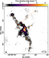 |
Fig. 1 Example of a 1.3 mm continuum image from the ASHES survey (Morii et al. 2023), overlaid with the NN graph (orange lines). The background colour scale and contours show the ALMA 12 m plus 7 m continuum emission, with contour levels at 3 × 2nσ (n = 0, 1, 2, . . .), where σ = 9.5 × 10⁻⁵ Jy beam−1 is the rms noise level. Detected core positions are marked by orange circles, and the scale bar in the lower left corresponds to 0.1 pc at the assumed distance 5.5 kpc. |
2 Model framework
To quantify the impact of projection on measured core separations, we constructed a set of simple three-dimensional toy models for the spatial distribution of dense cores. These models allowed us to compare the true intrinsic separations to their two-dimensional projected counterparts under controlled conditions, and to assess the statistical validity of the 4/π correction factor introduced above.
2.1 Core placement
We populate a region of characteristic radius R with N point-like “cores”. We consider two families of models:
(i) Spherical profiles. Isotropic distributions within a sphere of radius R, including a uniform baseline and several centrally concentrated profiles (Gaussian, power law, Plummer; see Appendix A). In the main text we focus on the uniform case, which provides a transparent baseline; the other profiles show very similar trends with modest shifts in absolute scale.
(ii) Hierarchical fractals (anisotropic). To capture clumpy, filamentary substructure, we generated fractal point sets following Cartwright & Whitworth (2004). A cube is recursively subdivided into ![Mathematical equation: $\[n_{\text {div}}^{3}\]$](/articles/aa/full_html/2026/03/aa58304-25/aa58304-25-eq7.png) cells; at each generation, cells are retained with probability
cells; at each generation, cells are retained with probability ![Mathematical equation: $\[p_{\text {keep}}=n_{\text {div }}^{D-3}\]$](/articles/aa/full_html/2026/03/aa58304-25/aa58304-25-eq8.png) , where D is the fractal dimension (0 < D ≤ 3). The recursion proceeds until the number of occupied cells exceeds the desired sampling size N by a comfortable margin (i.e. until the structure reaches sufficient multiplicity to populate the target number of points after pruning). We then optionally restrict the distribution to the inscribed sphere of radius R, rescale coordinates, and add small Gaussian jitter within final cells to break grid regularity. Lower D yields highly clumpy, anisotropic structures, whereas D → 3 approaches uniformity. Because the resulting geometry is not spherically symmetric, projected NN statistics can depend on viewing angle (see Sect. 3.4).
, where D is the fractal dimension (0 < D ≤ 3). The recursion proceeds until the number of occupied cells exceeds the desired sampling size N by a comfortable margin (i.e. until the structure reaches sufficient multiplicity to populate the target number of points after pruning). We then optionally restrict the distribution to the inscribed sphere of radius R, rescale coordinates, and add small Gaussian jitter within final cells to break grid regularity. Lower D yields highly clumpy, anisotropic structures, whereas D → 3 approaches uniformity. Because the resulting geometry is not spherically symmetric, projected NN statistics can depend on viewing angle (see Sect. 3.4).
2.2 Projection from 3D to 2D
Once generated, the 3D distribution is rotated by a chosen set of Euler angles (α, β, γ) and then projected onto the x–y plane by discarding the z coordinate. This procedure mimics the observational situation where only the sky-plane separations are accessible, while the line-of-sight dimension is collapsed.
2.3 Nearest neighbour analysis
For each configuration, we computed the NN graph in three dimensions and in the two-dimensional projection. Each core is linked to its single closest companion, producing a directed graph that can be collapsed into a set of unique, undirected edges. The output of the NN analysis consists of (i) the set of nearest-neighbour edges, i.e. the pairs of nodes identified as closest companions, and (ii) the length of each edge, corresponding to the minimum separation of each core.
For context, the MST is another pairwise graph used widely in clustering studies. While the NN graph isolates local proximity (sensitive to fragmentation scales), the MST enforces global connectivity and balances short and long links, making it well suited to tracing overall geometry and sub-clustering. We include MST-based comparisons alongside NN results in Appendix B to illustrate how projection affects global connectivity versus local spacing.
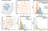 |
Fig. 2 Nearest-neighbour comparisons for N = 200 points drawn from a uniform spherical distribution within R = 1.0. Top: NN graph constructed in 3D, where the blue connections are the 3D NNs (left); 2D projection, where the orange connections are the 2D NNs (Centre); and the corresponding distributions of NN edge lengths (right) highlighting the overall shortening in projection. Bottom: detailed breakdown. The left panel repeats the 2D overlay of 3D and 2D edges, while the right panels show the distributions of ℓ3D, ℓ2D for shared edges and the ratios ℓ3D/ℓ2D. Vertical dashed lines mark the medians, and KDEs are overplotted on the histograms. Together these panels illustrate how projection both compresses lengths and reassigns neighbours, with only the very shortest pairs surviving unchanged. |
3 Model results
To isolate and understand the different factors that shape the observed NN statistics, we begin with the simplest possible case and then progressively add complexity. Starting from well sampled (N = 200) uniform random distributions establishes the geometric baseline against which all subsequent effects can be measured. We then explore how finite sampling the distribution and stochastic variance affect the stability of the NN network (varying N = 2–200), followed by how observational limitations alter its apparent topology. Finally, we examine a more physically motivated, hierarchical fractal distribution to assess how intrinsic substructure and orientation introduce additional, direction-dependent biases.
3.1 Uniform baseline: The simplest case
We started with the simplest model: a uniform 3D distribution of N = 200 points within a sphere of radius R = 1. Figure 2 shows the NN graph in 3D (top-left panel), the NN graph constructed from the projected points in 2D (top-middle panel), and the corresponding distributions of NN edge lengths (top-right panel). Projection immediately reduces the apparent neighbour separations to then give2,
![Mathematical equation: $\[\mathcal{C}=\frac{\left\langle\ell_{3 \mathrm{D}}\right\rangle}{\left\langle\ell_{2 \mathrm{D}}\right\rangle}=2.5 \quad(N=200),\]$](/articles/aa/full_html/2026/03/aa58304-25/aa58304-25-eq9.png)
which is far larger than the simple geometric expectation of 4/π ≃ 1.27.
The overlap between the 3D and projected 2D NN graphs is modest. Only about 20% of the 3D links are retained after projection, and the Jaccard similarity (J) is just 0.12 (the Jaccard similarity or index quantifies the fractional overlap between two sets, A and B, and is defined as J = |A ∩ B|/|A ∪ B|. It ranges from 0 for no shared elements, to 1 for identical sets). The few edges that survive in both graphs correspond mainly to the smallest true separations and remain strongly compressed, ⟨ℓ3D⟩/⟨ℓ2D⟩ ≃ 2.0, well above the geometric baseline of 4/π ≃ 1.27. Projection therefore shortens even the closest pairs substantially more than simple foreshortening alone.
Longer 3D connections are typically broken and replaced after projection. In the bottom-left panel of Fig. 2, the shared 3D-only edges that exist in the 3D NN graph but disappear in 2D (shown in blue) span relatively long intrinsic separations (⟨ℓ3D⟩3D-only ≃ 0.18), which project to ⟨ℓ2D⟩proj(3D-only) ≃ 0.153. These lost connections are almost always replaced in the projected NN graph by 2D-only edges (shown in orange in bottom-left panel of Fig. 2), i.e. new neighbours that appear only after projection. These are much shorter, with ⟨ℓ2D⟩2D-only ≃ 0.07. This behaviour is visible in the bottom-middle panel of Fig. 2, where the 2D-only histogram is concentrated at small scales compared to the projected 3D-only distribution. Quantitatively, the reassigned edges lie on average Δ⟨ℓ⟩ ≃ −0.08 below the projected lengths of the removed 3D-only links, and ~96% of 2D-only edges fall below the mean projected length of their 3D predecessors. Together, these trends confirm that projection into 2D space not only foreshortens individual separations but, more importantly, rewires the NN network by replacing long intrinsic links with new, much shorter projected neighbours, so that the apparent contraction of the 2D NN network is driven predominantly by systematic neighbour reassignment rather than pure geometric shortening.
As a complementary check, we can also ask what happens if the NN pairs themselves are forced to be fixed. When the same 3D pairs are forced to be measured in projection, the mean ratio drops slightly below the geometric value, ⟨ℓ3D/ℓ2D⟩forced = 1.1, indicating that pure foreshortening alone cannot reproduce the observed 2.5× contraction. This behaviour is seen in the bottom-right panel of Fig. 2, where the distribution of ℓ3D/ℓ2D for forced pairs (green) peaks near unity, while the shared-pair distribution (orange) extends to much larger ratios, tracing the stronger compression produced by reassignment. At the node level, only about 8% of points retain identical neighbours in 3D and 2D, demonstrating that projection reorganises the local topology of almost the entire network.
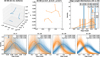 |
Fig. 3 Nearest-neighbour comparisons for uniformly sampled point distributions. Top: example realisation with N = 10 points drawn within a sphere of radius of R = 1.0. The NN graph constructed in 3D (left), its 2D projection obtained by dropping the line-of-sight coordinate (centre), and the corresponding edge-length distributions (right) illustrate how projection systematically shortens apparent separations and modifies the network connectivity even in a simple isotropic configuration. Bottom: results from the Monte Carlo ensembles (103 realisations each) for N = 5, 10, 20, and 50 showing stacked kernel density estimates of 3D (blue) and projected 2D (orange) NN edge lengths. The distributions converge at a stable median ratio as N increases, while stochastic fluctuations dominate at small values of N. |
3.2 Dependence on sample size
The structure of the NN network naturally depends on the number of sampled cores. To illustrate its behaviour in the simplest case, the upper panels of Fig. 3 shows an example for a uniform random distribution of N = 10 points within a sphere of radius R = 1.0. Even in such a statistically isotropic configuration, the 2D projection shortens the apparent edge lengths (median ratio ℓ3D/ℓ2D ≃ 1.6, closer to the geometric expectation of 4/π) and modifies the network topology: only about 57% of the 3D connections are recovered in projection (J = 0.36). Several intrinsic 3D links are replaced by shorter projected ones, reflecting how chance alignments and foreshortening affect the apparent connectivity. The example also highlights the stochasticity inherent to small–N realisations, where the precise NN configuration and the resulting length ratios vary between random draws of an identical underlying distribution.
The lower panels of Fig. 3 quantify how the projection bias depends on sample size for the uniform case using Monte Carlo ensembles (103 realisations per N). For each run we computed the ratio 𝒞(N) ≡ ⟨ℓ3D⟩/⟨ℓ2D⟩ and then characterised its distribution across the ensemble. The median ratio increases systematically with N, in line with the expected N1/6 scaling for Poisson samples (reflecting ⟨ℓ⟩ ∝ N−1/3 in 3D and N−1/2 in 2D). For example, we find 𝒞(N=5) = 1.50 ± 0.35 (16–84%: 1.20–1.79), 𝒞(N=10) = 1.65 ± 0.28 (1.39–1.91), 𝒞(N = 20) = 1.80 ± 0.23 (1.58–1.99), and 𝒞(N = 50) = 2.05 ± 0.16 (1.89–2.21), where the quoted uncertainties are the run-to-run scatter in 𝒞. As N increases the KDE stacks in the lower panels become smoother, the ensemble of 𝒞 values narrows, and the 3D and 2D distributions separate more cleanly. The latter is quantified by the Kolmogorov-Smirnov statistic D, which measures the maximum difference between the cumulative distributions: D rises from ≃0.3 at N=5 to ≃0.6 at N=50, indicating progressively stronger distinction between the 3D and 2D spacing distributions. Small-N realisations remain dominated by stochastic scatter, but by N ≳ 20 the median behaviour stabilises and the ensemble converges towards the combined geometric-statistical expectation, with 𝒞(N) well above the pure-projection baseline 4/π ≃ 1.27 due to the different N-scalings of ⟨ℓ⟩ in 3D and 2D.
 |
Fig. 4 Illustration of the impact of a finite SDR on NN statistics using a uniform distribution of N = 200 points within a sphere of radius R = 1.0. Left: intrinsic 3D NN graph. Centre: two-dimensional projection after applying a beam–blending step that merges points closer than one beam width, corresponding here to a SDR of SDR = FoV/FWHMbeam = 10. Circles mark the original 2D positions (open) and the resulting beam-blended centroids (filled). Right: distributions of NN edge lengths in 3D and 2D after blending. In this example, 135 of the 200 projected cores (67.5%) are merged into 65 effective groups, erasing all topological correspondence between the intrinsic and projected networks (J = 0.00, overlap fraction = 0). The typical 3D and 2D NN lengths become nearly equal (⟨ℓ3D⟩/⟨ℓ2D⟩ ≃ 1.0), as beam blending suppresses the shortest intrinsic separations that normally produce the geometric compression factor (4/π ≃ 1.27). This example illustrates that limited spatial resolution can strongly distort the apparent connectivity and scale distribution of dense cores even in an intrinsically uniform configuration. |
3.3 Impact of beam blending and spatial dynamic range
Real observations impose a finite spatial dynamic range (SDR) and, in practice, a limited ability to resolve close pairs. In this section we explicitly test how finite resolution and beam smoothing (i.e. confusion and blending) modify the NN network. For convenience, we express resolution through a single dimensionless parameter:
![Mathematical equation: $\[\mathrm{SDR} \equiv \frac{\mathrm{FoV}}{\mathrm{FWHM}_{\text {beam }}},\]$](/articles/aa/full_html/2026/03/aa58304-25/aa58304-25-eq10.png)
which simply measures how many synthesised beams fit across the field of view (FoV). This quantity can be rescaled straightforwardly to any instrument and setup. For instance, in an ALMA observation at 100 GHz, the primary beam has a full width half maximum (FWHM) of about 57″, so a single pointing imaged at 1″ resolution would have SDR ≈ 57 (mosaicked observations would have a larger FoV)4.
When the SDR is small (i.e. large FWHMbeam for fixed FoV), sources separated by less than a FWHMbeam cannot be distinguished as individual objects in projection and appear merged in the observed map. To mimic this observational limitation, we applied a simple beam-blending step after projecting the intrinsic 3D distribution: all points within one beam radius of each other are grouped together and replaced by a single blended source at their mean position. For the uniform example shown in Fig. 4, we adopted SDR = 10, corresponding to an effective resolution of 0.1 in our normalised units.
At N=200 within FoV = R = 1, introducing finite resolution through beam blending dramatically alters the NN network. For SDR = 10 (beam FWHM = FoV/10), any projected points closer than one beam are merged into a single centroid, mimicking the loss of distinct sources in observations. In this configuration, 135 of the 200 projected positions (67.5%) collapse into 65 blended groups, leaving only Neff = 65 nodes for the 2D NN graph. This coarse-graining removes precisely the shortest intrinsic separations (i.e. the pairs most likely to be genuine neighbours in 3D) and thus erases the topological correspondence between the intrinsic and projected networks; no 3D NN edges are recovered in 2D. At the same time, reducing the number of nodes inflates the characteristic 2D spacing.
Quantitatively, the intrinsic 3D NN length distribution has median = 0.179 (mean 0.176 ± 0.062), whereas the unsmoothed 2D projection has lengths median = 0.065 (mean 0.069 ± 0.021), reflecting strong projection compression (𝒞 ≃ 2.5; Section 3.1). After imposing finite resolution with SDR = 10, the adopted effective resolution scale is 1/10 = 0.1, and the beam-blended 2D distribution shifts to median = 0.168 (mean 0.173 ± 0.043). Because the resolution now exceeds the typical unsmoothed projected separations (⟨ℓ2D⟩unsm. ≈ 0.069 > 1), the beam systematically removes precisely the short NN links that dominated the projected network, merging close pairs into single centroids and truncating the short-end tail of the 2D NN distribution. As a result, the usual geometric compression seen under ideal projection largely disappears: the mean ratio collapses to 𝒞(SDR = 10) ≃ 1.0. In the unsmoothed case, by contrast, the same configuration yielded 𝒞 ≃ 2.5, with only ~20% of 3D NN edges surviving in projection and the rest replaced by much shorter 2D companions. Finite resolution therefore flips the regime from projection-dominated (shortening via neighbour reassignment) to resolution-dominated (coarse-graining via blending): the apparent network becomes nearly isometric while the intrinsic connectivity is erased.
3.4 Fractal, anisotropic structure: Orientation matters
To explore the impact of anisotropic, clumpy structure, we turn to a hierarchical fractal model that lacks spherical symmetry and whose projected NN statistics therefore depend on viewing angle. The distribution follows the Cartwright–Whitworth prescription with fractal dimension D = 1.6 and sub-division ndiv = 3 within a unit sphere (R = 1). Each generation divides space into ![Mathematical equation: $\[n_{\text {div}}^{3}\]$](/articles/aa/full_html/2026/03/aa58304-25/aa58304-25-eq11.png) cells and retains a fraction
cells and retains a fraction ![Mathematical equation: $\[n_{\text {div}}^{D-3}\]$](/articles/aa/full_html/2026/03/aa58304-25/aa58304-25-eq12.png) , producing a highly clumpy, cluster-like morphology typical of young stellar regions (e.g. Cartwright & Whitworth 2004 infer Taurus has D ~ 1.5), while remaining compact enough for robust sampling at fixed N. We initialise N=200 points and compare three orthogonal viewing angles (Fig. 5).
, producing a highly clumpy, cluster-like morphology typical of young stellar regions (e.g. Cartwright & Whitworth 2004 infer Taurus has D ~ 1.5), while remaining compact enough for robust sampling at fixed N. We initialise N=200 points and compare three orthogonal viewing angles (Fig. 5).
Projection again shortens apparent NN separations and rewires connectivity. For the full 2D networks, the mean compression (expressed as a ratio of mean lengths) spans
![Mathematical equation: $\[\frac{\left\langle\ell_{3 \mathrm{D}}\right\rangle}{\left\langle\ell_{2 \mathrm{D}}\right\rangle} \simeq 1.56{-}1.74\]$](/articles/aa/full_html/2026/03/aa58304-25/aa58304-25-eq13.png)
across the three orientations (from mean ℓ3D/ℓ2D = 1.56, 1.67, 1.74). The overlap between the 3D and 2D NN edge sets is moderate to high for a fractal. The fraction of 3D NN edges recovered in 2D is 0.51–0.59, and 32–43% of the nodes retain identical neighbour sets.
The pairs that survive in both graphs are intrinsically short and contract from ⟨ℓ3D⟩ ~ 0.033–0.036 to ⟨ℓ2D⟩ ~ 0.022–0.023, giving shared-edge ratios of
![Mathematical equation: $\[\left\langle\frac{\ell_{3 \mathrm{D}}}{\ell_{2 \mathrm{D}}}\right\rangle_{\text {shared }} \simeq 1.30{-}1.41.\]$](/articles/aa/full_html/2026/03/aa58304-25/aa58304-25-eq14.png)
By contrast, when the same 3D NN pairs are forced to be measured in projection, the mean ratios sit near unity,
![Mathematical equation: $\[\left\langle\frac{\ell_{3 \mathrm{D}}}{\ell_{2 \mathrm{D}}}\right\rangle_{\text {forced }} \simeq 0.87{-}0.97,\]$](/articles/aa/full_html/2026/03/aa58304-25/aa58304-25-eq15.png)
which is consistent with a pure-geometry baseline for fixed pairs.
The gap between the “shared” and “forced” behaviours again points to rewiring as the main driver of additional shortening: new 2D-only links are systematically shorter (median ℓ2D ≃ 0.016–0.023) than the projected lengths of the discarded 3D-only links (median ~0.035–0.040), with 75%-87% of 2D-only edges lying below the median projected scale of their lost 3D counterparts. Orientation changes the exact values but not the basic picture: lower D (more clumpy structure) produces slightly smaller global ⟨ℓ3D⟩/⟨ℓ2D⟩ than smoother, more uniform cases, but in all instances projection acts by both geometrically foreshortening separations and rewiring the NN network through neighbour reassignment.
4 Putting it all together: Dependence on structure, sampling, and resolution
Having examined the effects of projection, sampling statistics, and resolution separately, we now bring these ingredients together to assess how the NN projection bias depends jointly on the intrinsic structure, the sample size N, and the effective SDR. Our goal is to establish a compact, quantitative description of the mean distortion factor
![Mathematical equation: $\[\mathcal{C}(N, \mathrm{SDR}) \equiv \frac{\left\langle\ell_{3 \mathrm{D}}\right\rangle}{\left\langle\ell_{2 \mathrm{D}}\right\rangle},\]$](/articles/aa/full_html/2026/03/aa58304-25/aa58304-25-eq16.png)
and to determine how it varies across the physically relevant regimes for cluster and cloud observations.
We begin by isolating the dependence on N alone. Figure 6 shows the ensemble-averaged projection ratio for fractal realisations with dimensions D = 1.7–2.5 and sub-division levels ndiv = 2–4, each averaged over 1000 random realisations. The adopted range of fractal dimensions is intended to bracket a representative set of morphologies relevant for star-forming regions: lower values (D ~ 1.7) produce highly filamentary, strongly clustered structures, whereas higher values (D ~ 2.5) yield progressively more space-filling hierarchies. This choice is motivated by both numerical experiments of supersonic (approximately isothermal) turbulence and observational characterisations of molecular-cloud structure, which typically imply fractal dimensions in the broad range D ~ 1.8–2.7, with systematic variations depending on the tracer, analysis method, and the balance of solenoidal versus compressive driving (e.g. Elmegreen & Falgarone 1996; Sánchez et al. 2005, 2007; Federrath et al. 2009; Elia et al. 2014; Rathborne et al. 2015).
The solid curve in Figure 6 represents the mean across all configurations, while the dashed lines indicate the ±1σ scatter between configurations (not the run-to-run variance within a single setup). As in the uniform case (Sects. 3.1–3.2), the projection bias increases systematically with N, rising from ⟨ℓ3D⟩/⟨ℓ2D⟩ ~ 1.3 for very small samples to ~2.0–2.3 by N ≃ 200. This behaviour follows a sub-linear power law consistent with the geometric scaling ⟨ℓ⟩ ∝ N−1/3 in 3D versus N−1/2 in 2D, yielding an effective exponent β≃ 1/6. Higher fractal dimensions (i.e. smoother, more uniform point sets) tend to produce slightly larger ratios at fixed N, indicating that small-scale crowding and neighbour reassignment in the more clumpy (D ≃ 1.7) cases partially offset the pure geometric compression.
To disentangle the influence of spatial resolution, we next fix N = 200 and vary the spatial dynamic range for 1000 fractal realisations with D = 1.7–2.5, ndiv = 2–4 (Figure 7). At high SDR, the ratio saturates at 𝒞 ≈ 2.0, reflecting the intrinsic projection bias once individual cores are resolved. As SDR decreases, unresolved blending removes the shortest true separations, suppressing the apparent contraction until the 3D and 2D mean separations become comparable (𝒞 ≈ 1). This transition occurs around SDR ~ 20 for the fractal models, but its exact location depends on the underlying spatial hierarchy: lower-D distributions are affected at slightly higher SDR because their denser substructure contains more close pairs to be blended. The dependence of the projection ratio on fractal dimension at fixed (N, SDR), and the regime where structure and resolution become coupled, are examined in more detail in Appendix C.
Finally, to capture the combined dependence of the projection ratio on both sample size and spatial resolution, we modelled the full 2D surface 𝒞(N, SDR) with a compact functional form that separates the scaling with N from the saturation with dynamic range:
![Mathematical equation: $\[\mathcal{C}(N, \mathrm{SDR})=\mathcal{C}_{\infty}\left[1-\exp \left(-\mathrm{SDR} / S_0\right)\right]\left(\frac{N}{100}\right)^\beta.\]$](/articles/aa/full_html/2026/03/aa58304-25/aa58304-25-eq17.png) (6)
(6)
In this expression, 𝒞∞ represents the asymptotic projection ratio for large N and effectively infinite resolution, S0 defines the characteristic dynamic range at which finite beam size begins to suppress small-scale structure, and β quantifies the weak residual scaling with N. Note here that, when applying this relation to observations, N should be interpreted as the intrinsic three-dimensional population, such that using the observed N yields a conservative lower limit; further practical caveats are discussed in Sect. 5.1. Fitting this form to the grid of ensemble-averaged measurements from 1000 fractal realisations with D = 1.7–2.5, ndiv = 2–4 yields (see Figure 8)
![Mathematical equation: $\[\begin{aligned}\mathcal{C}_{\infty} & =1.94 \pm 0.01, \\S_0 & =21.8 \pm 0.3, \\\beta & =0.173 \pm 0.003.\end{aligned}\]$](/articles/aa/full_html/2026/03/aa58304-25/aa58304-25-eq18.png)
The S0 term marks the onset of significant blending for data with ~10–20 independent resolution elements across the field. The analytic fit reproduces the ensemble with a fractional residual of ~9%, indicating negligible systematic bias and excellent agreement with the mean trends in both N and SDR. To assess the intrinsic scatter around this mean relation, we separate (i) run-to-run Monte Carlo variation at fixed (N, SDR) from (ii) differences between fractal geometries.
The Monte Carlo scatter is modest, with a median fractional dispersion of ~0.17 (16–84% range 0.10–0.26). In contrast, geometric variations introduce a substantially larger spread: the median absolute deviation from the fitted surface is |Δ𝒞|/𝒞 ≃ 0.35 (16–84% range 0.12–1.19), and the full grid exhibits rare but extreme excursions up to max|Δ𝒞|/𝒞 ≃ 4.5. In practical terms, while the mean relation 𝒞(N, SDR) is constrained to better than ~10%, individual realisations of a fractal point distribution can differ from this mean by ~30–40% for typical geometries, occasionally reaching ~100% deviations, and in the most extreme sparse or strongly hierarchical cases, by factors of several (up to ~450%; see Figure 6).
In the limit of fully resolved observations (SDR → ∞), the exponential term in Equation (6) approaches unity, [1 − exp(−SDR/S0)] ≃ 1, and the relation simplifies to a purely sampling-dependent form:
![Mathematical equation: $\[\mathcal{C}(N)=1.94\left(\frac{N}{100}\right)^{0.173}.\]$](/articles/aa/full_html/2026/03/aa58304-25/aa58304-25-eq19.png) (7)
(7)
This expression captures the fundamental scaling of projection bias with sample size alone, independent of resolution effects, and reproduces the behaviour derived earlier for the idealised case (N1/6; see Sect. 1).
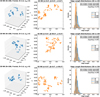 |
Fig. 5 Nearest-neighbour graphs for a fractal distribution with N = 200 points, fractal dimension D = 1.6, and sub-division ndiv = 3, within R = 1.0. Each row shows the NN network in 3D (left), the projected NN network in 2D (centre), and the corresponding NN edge-length distributions (right). The three rows illustrate different viewing geometries: no rotation (top), rotation about the y-axis (β = 90°; middle), and rotation about the z-axis (γ = 90°; bottom). Projection systematically shortens the apparent NN separations and rewires connectivity, but the degree of overlap and compression depends on the line of sight, reflecting the anisotropic and clumpy structure of the fractal distribution. |
 |
Fig. 6 Nearest-neighbour projection ratio ℓ3D/ℓ2D versus sample size N for fractal ensembles. For each N, we averaged 100 realisations per configuration and then combined across nine fractal setups (D ∈ {1.7, 2.0, 2.5}, ndiv ∈ {2, 3, 4}) with jitter=True and prune=True. The solid curve shows the cross-configuration mean, and the dashed curves indicate ±1σ across configurations (not the run-to-run uncertainty). The dashed horizontal line marks the geometric fixed-pair baseline 4/π ≃ 1.27. Projection bias is present at all N, with ℓ3D/ℓ2D increasing sub-linearly with N and reaching ~2.0–2.3 by N = 200, depending on fractal parameters. A higher D (less clumpy) yields larger ratios at a fixed N, indicating that beyond geometric compression, crowding and neighbour reassignment drive additional shortening in projection. |
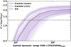 |
Fig. 7 Nearest-neighbour projection ratio ⟨ℓ3D⟩/⟨ℓ2D⟩ as a function of SDR evaluated for fractal ensembles (D = 1.7–2.5, ndiv = 2–4) at a fixed value of N = 200. Points and shaded bands show the mean and ±1σ scatter across configurations. The projection bias increases rapidly up to SDR ~ 10–20, beyond which it asymptotically approaches the intrinsic structural limit (𝒞∞ ≈ 1.9–2.0). At a low SDR, beam blending dominates, merging close pairs and driving 𝒞 → 1, i.e. apparent isometry between 3D and 2D separations. |
5 Discussion
Projection alters NN statistics by both foreshortening true separations and rewiring the NN graph. Many intrinsic 3D neighbours are replaced by closer projected companions, so ⟨ℓ3D⟩/⟨ℓ2D⟩ systematically exceeds the geometric baseline 4/π ≃ 1.27 and grows sub-linearly with sample size. Finite angular resolution adds a competing effect: when the spatial dynamic range SDR ≡ FoV/FWHMbeam is modest, beam blending merges sources within roughly one beam, removing the shortest links and inflating the apparent 2D separations so that 𝒞 is driven back towards unity as the characteristic NN scale approaches the beam. These trends are captured by our empirical surface (Eq. (6)), where 𝒞∞ = 1.94 is the large-N, infinite-resolution plateau, β ≃ 0.173 matches the expected N1/6 scaling, and S0 ≃ 21.8 marks the dynamic-range threshold where blending becomes important.
Table 1 turns the fitted surface 𝒞(N, SDR) into a set of ready-to-use numbers, organised by sampling (N) and SDR. Three regimes are evident:
(i) Low N or coarse resolution (N ≲ 10 or SDR ≲ 10): Beam blending removes the shortest intrinsic links, and 𝒞 sits near unity, so geometric de-projection alone is inadequate;
(ii) Intermediate (N ~ 20–100, SDR ~ 20–50): 𝒞 rises quickly as projection-induced rewiring dominates, while the resolution already resolves most pairs. This is the transition zone where comparing maps of different angular resolutions without correction can bias conclusions;
(iii) Well-sampled, well-resolved (N ≳ 100, SDR ≳ 50): 𝒞 approaches the large-N plateau ~eq2, with weak additional gains from increasing N or SDR.
The second and third header rows in the table map SDR to the beam FWHM (for an ALMA primary beam of 57″ at 100 GHz) and to a physical resolution for a 1 pc field at 3.6 kpc, allowing observers to locate their datasets in the table directly. In practice, one chooses the row matching the N and the column closest to the SDR (or beam FWHM divided by physical resolution) and applies 𝒞 as a multiplicative correction to convert measured 2D NN spacings to an approximate 3D mean. Differences on the order of 40% between morphologies and orientations set a sensible systematic floor for error budgets. Within that tolerance, the tabulated values provide a concise, physically motivated correction across typical ALMA setups.
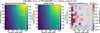 |
Fig. 8 Combined dependence of the projection distortion ratio 𝒞(N, SDR) = ⟨ℓ3D⟩/⟨ℓ2D⟩ on sample size N and SDR. Left: ensemble-averaged measurements from 1000 fractal realisations with D = 1.7–2.5 and ndiv = 2–4. Centre: best-fitting three-parameter model 𝒞∞[1 − e−SDR/S0](N/100)β. Right: fractional residuals (𝒞meas − 𝒞fit)/𝒞fit. The fitted parameters (𝒞∞ = 1.94, S0 = 21.8, β = 0.17) capture the joint behaviour across two orders of magnitude in both variables. The model converges to the geometric projection limit (𝒞 ≃ 1.3) for small well-resolved samples and to the beam-limited regime (𝒞 ≃ 1) when SDR ≲ 10. |
5.1 Comparison to observations
To quantify how the choice of correction factor influences the inferred fragmentation scale, we applied the derived relations to the ASHES sample (Morii et al. 2024), which contains 839 dense cores across 39 IRDCs (~20 cores per region; N varies from 8 to 39). For each region, we estimated the implied 3D NN separations using both the sample-size-dependent correction given by Eq. (7) and the resolution-dependent form in Eq. (6), where the spatial dynamic range SDR is defined as the ratio of host clump radius (see Morii et al. 2024) to beam FWHM (~ 1″), and varies between 10 and 40. The resulting distributions are shown in Figure 9.
The statistics illustrate how each correction systematically alters the spacing distribution. The uncorrected (projected) separations have a mean of 0.096 pc and a median of 0.077 pc. Applying the 𝒞(N) correction increases these to 0.14 pc and 0.12 pc, respectively, broadening the distribution and shifting the median upward by roughly 50%. This corresponds to a mean ratio of 1.50, consistent with the ensemble prediction for N ~ 20. In contrast, incorporating the finite dynamic range via 𝒞(N, SDR) lowers the mean and median back to 0.089 and 0.073 pc, respectively – effectively reducing the inferred 3D separations by ~40% relative to the 𝒞(N) case. This reversal arises because, for the ASHES data, the beam size is comparable to the typical NN spacing (SDR ~ 10–20). Beam blending therefore suppresses the shortest separations and counteracts the geometric expansion produced by projection correction.
The implications of this result are subtle but important. In Morii et al. (2024), the observed (projected) core separations were found to be comparable to the thermal Jeans length of the parent clumps, leading to the interpretation that fragmentation proceeds predominantly at the thermal, rather than turbulent, Jeans scale. Applying the 𝒞(N) correction increases the median spacing from 0.077 pc to 0.12 pc, raising the ratio δsep/λJ from 0.7 to ~1.2. This suggests that the intrinsic 3D separations are slightly larger than the thermal Jeans length, which is still consistent with thermally regulated fragmentation, but with less room for turbulent support. When finite angular resolution is included through 𝒞(N, SDR), the median spacing shifts back towards the uncorrected value (0.073 pc), maintaining δsep/λJ ≃ 0.9. However, this apparent “agreement” arises for the wrong reason: the dynamic-range correction suppresses separations because beam blending merges unresolved substructure into fewer larger nodes. This highlights an important warning for interpreting core spacings in marginally resolved maps, when the typical NN separation approaches the beam FWHM, a substantial fraction of the small-scale structure may remain unresolved, leading to biased estimates of both the physical spacing and the inferred fragmentation mode. In such cases, apparent consistency with the Jeans length does not necessarily confirm thermal fragmentation, but may instead reflect the observational limits of resolution and completeness.
We stress that this application is illustrative. In particular, the corrections are evaluated using the observed number of cores and an effective clump radius, whereas the intrinsic 3D sample size, geometry, and completeness are not known. As a result, the quoted 3D spacings should be treated as approximate and, if Nobs < Ntrue, as lower limits on the true projection factor and intrinsic separation, with systematic uncertainties of at least 30–40% from the underlying morphology (see Sect. 5.3).
Fitted projection-correction factors 𝒞(N, SDR) from the empirical relation 𝒞(N, SDR) = 𝒞∞[1 − e−SDR/S0](N/100)β using 𝒞∞ = 1.94, S0 = 21.8, and β = 0.173.
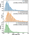 |
Fig. 9 Effect of projection and resolution corrections on the distribution of NN separations in the ASHES survey (Morii et al. 2024). Top: Observed (projected) 2D separations. Middle: Separations corrected for projection bias using the Sample-size-dependent relation 𝒞(N) (Eq. (7)). Bottom: Separations corrected for both projection and finite angular resolution using 𝒞(N, SDR) (Eq. (6)). Dashed lines mark the median values in each panel. The uncorrected distribution peaks near 0.08 pc, increases to 0.12 pc after applying 𝒞(N), but returns to 0.07 pc when the finite dynamic range (SDR ~ 10–20, defined as clump radius to beam FWHM) is included. This demonstrates the competing influences of geometric projection, which lengthens apparent separations, and beam blending, which suppresses the shortest scales (note the caveats of applying this correction to observations in Sect. 5.3). |
5.2 Comparison to simulations
In simulations of star formation, and the subsequent dynamical evolution of star-forming regions, the spatial distributions of the stars are often quantified using NN analyses (e.g. Klessen & Kroupa 2001; Schmeja & Klessen 2006; Schmeja 2011; Parker & Wright 2018) and MST analyses (Allison et al. 2010; Kirk et al. 2014; Parker et al. 2014; Domínguez et al. 2017; Parker et al. 2024). For the majority of measured diagnostics (e.g. Q-parameter, or the ΛMSR measure of mass segregation), the simulations can simply be analysed in 2D in the same way an observed star-forming region is. Often, a perfunctory check is made in a different plane (e.g. z–x rather than x–y) to establish that the measurement is also significant from a different viewing angle, but diagnostics such as 𝒬 and ΛMSR were designed specifically for analysis of 2D data and no conversion between two and three dimensions is performed.
However, similar clump-finding, or cluster-finding, algorithms are applied to simulation data as are applied to observed data (e.g. Guszejnov et al. 2022), and similar issues arise in identifying structures in 2D rather than the true underlying three-dimensional distribution. Again, simulations can be analysed in the same number of dimensions available to observers (usually two), but as we have shown the two-dimensional structures identified may not accurately reflect the underlying distribution. For example, Parker & Wright (2018) apply a Friends of Friends algorithm (which is a NN based algorithm) to N-body simulation data and identify groups in three dimensions, but in different projections the groups they identified in the x–y plane were not always apparent in two dimensions in the z–x and z–y planes.
Parker & Wright (2018) identified a further issue that is often overlooked in clump or cluster-finding algorithms, namely that clumpy and sub-clustered distributions may be self-similar on all scales (e.g. fractal), in which case identifying groups via, for example, an MST or NN method can become meaningless.
Gutermuth et al. (2009) used a technique for identifying sub-clusters and substructures by constructing a MST of a star-forming region, and then analysing the distribution of MST branch lengths. They fit two lines to the distribution; one fitting the smallest branch lengths, and the other fitting the largest branch lengths. Where these two lines intersect is taken to be an indication of where small-scale structure changes to large-scale structure, and all branch lengths longer than this are removed in the full MST, leaving multiple smaller groups.
However, Parker & Goodwin (2015) find that if the distribution of branch lengths is plotted on a logarithmic axis, there is no obvious break length, which is due to the fractal distribution being similar on all scales. If there is no true break in an observed distribution, i.e. if it is self-similar on all scales (e.g. fractal), then any groups identified by this (or a similar technique) may not have any physical significance. This illustrates the pitfalls of over-interpreting these data, even when all of the three-dimensional information is available, such as in simulations.
5.3 Caveats and future avenues of research
Our analysis was deliberately focused on idealised toy models in order to isolate the geometric effects of projection. Several caveats are worth highlighting.
Point-like cores. Real dense cores have finite sizes determined by both the instrumental beam and their intrinsic density structure. Beam convolution, blending, and spatial filtering inevitably modify the observed core distribution, while cores sit atop a complex, non-uniform background of cloud emission. This makes their detection and deblending sensitive to the local surface-brightness field and to the specific core-identification algorithm employed. In projection, such effects can cause multiple nearby cores in 3D to merge into a single 2D source or, conversely, to fragment spurious subcomponents from structured noise. Both processes distort the recovered NN distribution and may either dilute or amplify the apparent projection bias.
Sensitivity limits. Finite sensitivity and noise variations lead to incompleteness, particularly for faint or compact cores near the detection threshold. This effectively reduces the observable sample size and increases the measured mean separation by removing the (smallest) pairs. For a randomly thinned population, the average NN separation scales roughly as
![Mathematical equation: $\[\left\langle\ell_{2 \mathrm{D}}\right\rangle \propto N_{\text {eff}}^{-1 / 2}\]$](/articles/aa/full_html/2026/03/aa58304-25/aa58304-25-eq20.png) , so even moderate incompleteness (10–30%) can inflate apparent separations by tens of percent.
, so even moderate incompleteness (10–30%) can inflate apparent separations by tens of percent.Background confusion and structured emission. Inhomogeneous cloud emission or absorption can produce spatially varying completeness across the field, selectively obscuring compact or blended sources in crowded regions. This effect preferentially removes the shortest projected separations (i.e. those most likely to represent true physical neighbours) thereby biasing the apparent spacing distribution towards larger values. Such environment-dependent incompleteness acts in the same direction as beam blending, but with stronger spatial correlation and greater potential to distort clustering statistics near bright ridges or filaments.
Field of view and spatial coverage. The effective FoV sets how much of a clump or cloud contributes to the statistics and therefore directly influences the apparent sample size, N. Throughout this work we implicitly assume a single clump roughly enclosed by the observations (e.g. one ALMA primary beam). In practice, mosaics and primarybeam attenuation can truncate peripheral emission or omit outer cores belonging to the same parent structure. This censors the longest separations and narrows the observed spacing distribution. This then means that the observation strategy could matter. Wide mosaics such as ALMA-IMF typically deliver N ≳ 100–200 cores per field (Motte et al. 2022), whereas single-pointing studies such as ASHES often yield N ~ 10–30 per clump (Morii et al. 2024). Even if the core surface density is comparable, a larger FoV raises the measured N, and if used naively in Eq. (6), it increases the inferred correction purely because more area was included. Likewise, the mosaic FoV also increases the spatial dynamic range, SDR = FoV/FWHMbeam, pushing 𝒞(N, SDR) closer to its asymptote. Thus, N (and SDR) are observationally dependent quantities unless defined per a fixed aperture.
Idealised morphologies. The models explored here are spherically symmetric or statistically isotropic fractals designed to isolate geometric effects. Real star-forming regions, however, contain filaments, hubs, and hierarchical networks of substructure. Orientation-dependent projection of such anisotropic features can alter the observed NN statistics, typically changing 𝒞 by 10–20% but potentially more for strongly elongated geometries (e.g. end-on filaments or sheets seen nearly face-on). These departures highlight that while our calibration captures the dominant sampling and crowding effects, detailed modelling may be required for strongly anisotropic morphologies.
Intrinsic versus observed sample size. Finally, our calibration is expressed in terms of the intrinsic number of objects N in the 3D distribution, whereas observations only provide the number of detected cores, Nobs. Incomplete detection (due to sensitivity, blending, or limited FoV mentioned above) implies Nobs ≤ N, so using Nobs in Eq. (6) systematically underestimates 𝒞(N, SDR) and hence the inferred 3D separations. In this sense, corrections based on the observed Nobs should be regarded as conservative lower limits. A more rigorous application would estimate an effective intrinsic N – for example via completeness corrections or priors on the core surface density within a fixed physical aperture – before evaluating 𝒞(N, SDR).
These caveats point naturally to several avenues for future work:
Simulations. Extending the NN projection analysis to full magneto-hydrodynamic simulations can test whether the empirical calibration remains valid once realistic physics (e.g. gravity, turbulence, feedback, and magnetic fields) shape the spatial and kinematic distribution of cores (e.g. Lebreuilly et al. 2025; Tung et al. 2025; Nucara et al. 2025). These tests would also quantify how fragmentation geometry and crowding evolve dynamically, allowing the derived 𝒞(N, SDR) relation to be linked to physical time-scales and evolutionary stages.
Forward modelling of observed regions. For individual molecular clouds with modellable geometry (e.g. filamentary or Hub-filament systems), tailored mock observations can be used to constrain the orientation dependence C(N, i) as a function of inclination and line-of-sight structure.
Finite resolution and beam blending. A realistic treatment should “smooth” the projected (2D) maps with an instrumental beam so that cores are no longer point-like, and then recover their distribution using standard, observation-driven tools (e.g. Astrodendro dendrograms, GETSF, CUTEX, CLUMPFIND). Beam convolution and spatial filtering merge nearby emission peaks, suppress the shortest separations, and reduce the effective count of recovered objects, driving 𝒞(N, SDR) towards unity. Systematically varying the taper, clean beam, and deblending thresholds in such synthetic pipelines would calibrate where the transition occurs and refine the empirical parameter S0 that marks the onset of blending in our model.
Field of view, spatial coverage, and completeness. In this work we treat each field as a single clump, but in practice N also depends on FoV so parameterising the correction by the core surface density Σcore or a matched physical aperture provides a more consistent comparison across datasets. Practical ways forward include (i) reporting both N and Σcore, along with distance and beam FWHM; (ii) applying 𝒞(N, SDR) using an N measured within a matched physical or angular aperture when comparing regions with differing FoV; and (iii) re-evaluating 𝒞 across nested apertures to assess sensitivity to coverage. Synthetic experiments that vary FoV at fixed Σcore and SDR can quantify how coverage-induced changes in N propagate into 𝒞(N, SDR) and establish robust comparison practices between narrow- and wide-field surveys. Finally, comparisons with numerical simulations of evolving clusters–where physical core disruption and migration can modify apparent completeness–could help disentangle observational incompleteness from genuine dynamical evolution, and motivate a future re-parameterisation of the correction in terms of both Σcore and evolutionary state.
Incorporating kinematic priors. Future extensions could link cores not only in projected space but also in velocity space, using the assumption that objects close in vLSR are more likely to be physically associated. Such tests would constrain additional priors on the spatial distribution and refine the estimation of true 3D separations.
Testing line-of-sight reconstruction methods. Because the intrinsic 3D positions are known in our simulations, this framework provides an ideal benchmark for evaluating MCMC-based reconstruction approaches such as those proposed by Svoboda et al. (2019) and Traficante et al. (2023).
Applications beyond dense cores. Since NN statistics are widely used in stellar clustering, galaxy surveys, and largescale structure analyses, repeating this exercise in those contexts can test the generality and universality of the derived projection corrections.
6 Conclusions
We have quantified how projection and finite resolution bias the NN statistics commonly used to characterise spatial structure in star-forming regions. Using idealised three-dimensional distributions, we showed that the mean ratio of intrinsic to projected NN separations, 𝒞 ≡ ⟨ℓ3D⟩/⟨ℓ2D⟩, systematically exceeds the simple geometric expectation, 4/π, once the sample contains more than a handful of objects. As the number of points increases, projection not only foreshortens individual separations, but it also rewires the NN network, replacing many true 3D links with new shorter 2D neighbours. Finite angular resolution adds a second, opposing bias: Smoothing and beam blending merge intrinsically distinct cores into single sources, effectively reducing the number of independent points and inflating the apparent separations. Taken together, these effects erase most of the original three-dimensional connectivity. The observed 2D NN graph preserves only a coarse shadow of the underlying structure, and there is no simple global geometry, which is the only factor that can recover the true 3D network from projected separations.
We attempted to capture the combined behaviour of the competing effects of crowding versus resolution through an empirical relation,
![Mathematical equation: $\[\mathcal{C}(N, \mathrm{SDR})=\mathcal{C}_{\infty}\left[1-\exp \left(-\mathrm{SDR} / S_0\right)\right]\left(\frac{N}{100}\right)^\beta,\]$](/articles/aa/full_html/2026/03/aa58304-25/aa58304-25-eq21.png)
with 𝒞∞ = 1.94, S0 = 21.8, and β = 0.173. This relation reproduces the ensemble-averaged simulation results to within ~10%. Individual realisations, however, can deviate by ~30–40% on average, and in rare cases by factors of a few, owing to stochastic variations in fractal geometry and sampling. The relation spans the physically relevant range 𝒞 ≃ 1–2.3 from unresolved, beamdominated regimes (where blending drives 𝒞 → 1 and the NN network is almost completely destroyed and rewired) to well-resolved, well-sampled regimes in which projection-induced rewiring pushes 𝒞 towards its asymptotic plateau, 𝒞∞ ≃ 2. For practical use, this calibration was implemented in the publicly available corespacing3d package, which provides a convenience function to evaluate 𝒞(N, SDR) for arbitrary parameter choices (Barnes & Henshaw 2026).
This work represents a first step towards a unified treatment of projection bias in spatial statistics. By construction it is deliberately simplified, omitting several important factors–such as sensitivity limits, background confusion, strongly anisotropic morphologies, and incomplete field coverage–that can further distort observed core distributions. The caveats we highlighted show that two-dimensional separations should be interpreted with caution, as they reflect a convolution of intrinsic structure, sampling, and observational bias, and that apparent agreement with theoretical scales (e.g. a Jeans length) does not guarantee a one-to-one physical correspondence. Our calibration provides a foundation for addressing these effects systematically. Future efforts should incorporate synthetic observations of hydrodynamic simulations, explicit sensitivity and completeness cuts, and orientation-dependent extensions, ultimately enabling a more physically consistent comparison between observed and intrinsic fragmentation scales.
Acknowledgements
We are grateful to the referee, Nestor Sanchez, for their constructive suggestions. This work grew out of conversations at the Stellar Origins 2025 meeting in Vienna. I thank the organisers for creating such a productive environment and the many colleagues who offered thoughtful feedback during and after the meeting. RJP acknowledges support from the Royal Society in the form of a Dorothy Hodgkin fellowship.
References
- Allison, R. J., Goodwin, S. P., Parker, R. J., Portegies Zwart, S. F., & de Grijs, R. 2010, MNRAS, 407, 1098 [NASA ADS] [CrossRef] [Google Scholar]
- Avison, A., Fuller, G. A., Frimpong, N. A., et al. 2023, MNRAS, 526, 2278 [Google Scholar]
- Barnes, A. T., & Henshaw, J. 2026, corespaceing3d [Google Scholar]
- Barnes, A. T., Henshaw, J. D., Fontani, F., et al. 2021, MNRAS, 503, 4601 [CrossRef] [Google Scholar]
- Beuther, H., Henning, T., Linz, H., et al. 2015, A&A, 581, A119 [NASA ADS] [CrossRef] [EDP Sciences] [Google Scholar]
- Beuther, H., Mottram, J. C., Ahmadi, A., et al. 2018, A&A, 617, A100 [NASA ADS] [CrossRef] [EDP Sciences] [Google Scholar]
- Beuther, H., Gieser, C., Suri, S., et al. 2021, A&A, 649, A113 [NASA ADS] [CrossRef] [EDP Sciences] [Google Scholar]
- Cartwright, A., & Whitworth, A. P. 2004, MNRAS, 348, 589 [Google Scholar]
- Casertano, S., & Hut, P. 1985, ApJ, 298, 80 [Google Scholar]
- Chevance, M., Krumholz, M. R., McLeod, A. F., et al. 2023, in Astronomical Society of the Pacific Conference Series, 534, Protostars and Planets VII, eds. S. Inutsuka, Y. Aikawa, T. Muto, K. Tomida, & M. Tamura, 1 [Google Scholar]
- Clark, P. J., & Evans, F. C. 1954, Ecology, 35, 445 [Google Scholar]
- Domínguez, R., Fellhauer, M., Blaña, M., Farias, J. P., & Dabringhausen, J. 2017, MNRAS, 472, 465 [CrossRef] [Google Scholar]
- Elia, D., Strafella, F., Schneider, N., et al. 2014, ApJ, 788, 3 [Google Scholar]
- Elmegreen, B. G., & Falgarone, E. 1996, ApJ, 471, 816 [NASA ADS] [CrossRef] [Google Scholar]
- Federrath, C., & Klessen, R. S. 2012, ApJ, 761, 156 [Google Scholar]
- Federrath, C., Klessen, R. S., & Schmidt, W. 2009, ApJ, 692, 364 [Google Scholar]
- Guszejnov, D., Markey, C., Offner, S. S. R., et al. 2022, MNRAS, 515, 167 [NASA ADS] [CrossRef] [Google Scholar]
- Gutermuth, R. A., Megeath, S. T., Myers, P. C., et al. 2009, ApJS, 184, 18 [Google Scholar]
- Hacar, A., Clark, S. E., Heitsch, F., et al. 2023, in Astronomical Society of the Pacific Conference Series, 534, Protostars and Planets VII, eds. S. Inutsuka, Y. Aikawa, T. Muto, K. Tomida, & M. Tamura, 153 [Google Scholar]
- Hartmann, L. 2002, ApJ, 578, 914 [Google Scholar]
- Hartmann, L., Ballesteros-Paredes, J., & Bergin, E. A. 2001, ApJ, 562, 852 [NASA ADS] [CrossRef] [Google Scholar]
- Hennebelle, P., & Inutsuka, S.-i. 2019, Front. Astron. Space Sci., 6, 5 [Google Scholar]
- Henshaw, J. D., Caselli, P., Fontani, F., et al. 2016, MNRAS, 463, 146 [NASA ADS] [CrossRef] [Google Scholar]
- Henshaw, J. D., Jiménez-Serra, I., Longmore, S. N., et al. 2017, MNRAS, 464, L31 [Google Scholar]
- Inutsuka, S.-i., & Miyama, S. M. 1997, ApJ, 480, 681 [NASA ADS] [CrossRef] [Google Scholar]
- Ishihara, K., Sanhueza, P., Nakamura, F., et al. 2024, ApJ, 974, 95 [NASA ADS] [CrossRef] [Google Scholar]
- Jeans, J. H. 1902, Philos. Trans. Roy. Soc. Lond. Ser. A, 199, 1 [NASA ADS] [CrossRef] [Google Scholar]
- Jiao, W., Wang, K., Pillai, T. G. S., et al. 2023, ApJ, 945, 81 [NASA ADS] [CrossRef] [Google Scholar]
- Kainulainen, J., Hacar, A., Alves, J., et al. 2016, A&A, 586, A27 [NASA ADS] [CrossRef] [EDP Sciences] [Google Scholar]
- Kainulainen, J., Stutz, A. M., Stanke, T., et al. 2017, A&A, 600, A141 [NASA ADS] [CrossRef] [EDP Sciences] [Google Scholar]
- Kirk, H., & Myers, P. C. 2011, ApJ, 727, 64 [Google Scholar]
- Kirk, H., Offner, S. S. R., & Redmond, K. J. 2014, MNRAS, 439, 1765 [Google Scholar]
- Klessen, R. S., & Kroupa, P. 2001, A&A, 372, 105 [NASA ADS] [CrossRef] [EDP Sciences] [Google Scholar]
- Lada, C. J., & Lada, E. A. 2003, ARA&A, 41, 57 [Google Scholar]
- Larson, R. B. 1985, MNRAS, 214, 379 [NASA ADS] [Google Scholar]
- Lebreuilly, U., Traficante, A., Nucara, A., et al. 2025, A&A, 701, A217 [NASA ADS] [CrossRef] [EDP Sciences] [Google Scholar]
- Liu, H. B., Chen, H.-R. V., Román-Zúniga, C. G., et al. 2019, ApJ, 871, 185 [NASA ADS] [CrossRef] [Google Scholar]
- Lu, X., Cheng, Y., Ginsburg, A., et al. 2020, ApJ, 894, L14 [NASA ADS] [CrossRef] [Google Scholar]
- Molinari, S., Schilke, P., Battersby, C., et al. 2025, A&A, 696, A149 [NASA ADS] [CrossRef] [EDP Sciences] [Google Scholar]
- Morii, K., Sanhueza, P., Nakamura, F., et al. 2023, ApJ, 950, 148 [NASA ADS] [CrossRef] [Google Scholar]
- Morii, K., Sanhueza, P., Zhang, Q., et al. 2024, ApJ, 966, 171 [Google Scholar]
- Motte, F., Bontemps, S., Csengeri, T., et al. 2022, A&A, 662, A8 [NASA ADS] [CrossRef] [EDP Sciences] [Google Scholar]
- Myers, P. C. 2017, ApJ, 838, 10 [NASA ADS] [CrossRef] [Google Scholar]
- Nucara, A., Traficante, A., Lebreuilly, U., et al. 2025, A&A, 701, A219 [NASA ADS] [CrossRef] [EDP Sciences] [Google Scholar]
- Offner, S. S. R., Moe, M., Kratter, K. M., et al. 2023, in Astronomical Society of the Pacific Conference Series, 534, Protostars and Planets VII, eds. S. Inutsuka, Y. Aikawa, T. Muto, K. Tomida, & M. Tamura, 275 [Google Scholar]
- Padoan, P., & Nordlund, Å. 2002, ApJ, 576, 870 [NASA ADS] [CrossRef] [Google Scholar]
- Palau, A., Ballesteros-Paredes, J., Vázquez-Semadeni, E., et al. 2015, MNRAS, 453, 3785 [Google Scholar]
- Palau, A., Zapata, L. A., Román-Zúniga, C. G., et al. 2018, ApJ, 855, 24 [NASA ADS] [CrossRef] [Google Scholar]
- Parker, R. J., & Goodwin, S. P. 2015, MNRAS, 449, 3381 [Google Scholar]
- Parker, R. J., & Wright, N. J. 2018, MNRAS, 481, 1679 [Google Scholar]
- Parker, R. J., Wright, N. J., Goodwin, S. P., & Meyer, M. R. 2014, MNRAS, 438, 620 [Google Scholar]
- Parker, R. J., Pinson, E. J., Alcock, H. L., & Dale, J. E. 2024, ApJ, 974, 8 [Google Scholar]
- Pineda, J. E., Arzoumanian, D., Andre, P., et al. 2023, in Astronomical Society of the Pacific Conference Series, 534, Protostars and Planets VII, eds. S. Inutsuka, Y. Aikawa, T. Muto, K. Tomida, & M. Tamura, 233 [Google Scholar]
- Plunkett, A., Hacar, A., Moser-Fischer, L., et al. 2023, PASP, 135, 034501 [NASA ADS] [CrossRef] [Google Scholar]
- Pokhrel, R., Myers, P. C., Dunham, M. M., et al. 2018, ApJ, 853, 5 [NASA ADS] [CrossRef] [Google Scholar]
- Pouteau, Y., Motte, F., Nony, T., et al. 2023, A&A, 674, A76 [NASA ADS] [CrossRef] [EDP Sciences] [Google Scholar]
- Rathborne, J. M., Longmore, S. N., Jackson, J. M., et al. 2015, ApJ, 802, 125 [Google Scholar]
- Rebolledo, D., Guzmán, A. E., Contreras, Y., et al. 2020, ApJ, 891, 113 [Google Scholar]
- Rosen, A. L., Offner, S. S. R., Sadavoy, S. I., et al. 2020, Space Sci. Rev., 216, 62 [Google Scholar]
- Sánchez, N., Alfaro, E. J., & Pérez, E. 2005, ApJ, 625, 849 [CrossRef] [Google Scholar]
- Sánchez, N., Alfaro, E. J., & Pérez, E. 2007, ApJ, 656, 222 [CrossRef] [Google Scholar]
- Sanhueza, P., Contreras, Y., Wu, B., et al. 2019, ApJ, 886, 102 [Google Scholar]
- Schisano, E., Molinari, S., Coletta, A., et al. 2026, A&A, in press, https://doi.org/10.1051/0004-6361/202555619 [Google Scholar]
- Schmalzl, M., Kainulainen, J., Quanz, S. P., et al. 2010, ApJ, 725, 1327 [NASA ADS] [CrossRef] [Google Scholar]
- Schmeja, S. 2011, Astron. Nachr., 332, 172 [NASA ADS] [CrossRef] [Google Scholar]
- Schmeja, S., & Klessen, R. S. 2006, A&A, 449, 151 [NASA ADS] [CrossRef] [EDP Sciences] [Google Scholar]
- Schmeja, S., Klessen, R. S., & Froebrich, D. 2005, A&A, 437, 911 [NASA ADS] [CrossRef] [EDP Sciences] [Google Scholar]
- Schneider, S., & Elmegreen, B. G. 1979, ApJS, 41, 87 [Google Scholar]
- Svoboda, B. E., Shirley, Y. L., Traficante, A., et al. 2019, ApJ, 886, 36 [Google Scholar]
- Tafalla, M., & Hacar, A. 2015, A&A, 574, A104 [NASA ADS] [CrossRef] [EDP Sciences] [Google Scholar]
- Teixeira, P. S., Takahashi, S., Zapata, L. A., & Ho, P. T. P. 2016, A&A, 587, A47 [NASA ADS] [CrossRef] [EDP Sciences] [Google Scholar]
- Thomasson, B., Joncour, I., Moraux, E., et al. 2022, A&A, 665, A119 [NASA ADS] [CrossRef] [EDP Sciences] [Google Scholar]
- Thomasson, B., Joncour, I., Moraux, E., et al. 2024, A&A, 689, A133 [NASA ADS] [CrossRef] [EDP Sciences] [Google Scholar]
- Traficante, A., Jones, B. M., Avison, A., et al. 2023, MNRAS, 520, 2306 [NASA ADS] [CrossRef] [Google Scholar]
- Tung, N.-D., Traficante, A., Lebreuilly, U., et al. 2025, A&A, 701, A218 [NASA ADS] [CrossRef] [EDP Sciences] [Google Scholar]
- Wright, N. J., Kounkel, M., Zari, E., Goodwin, S., & Jeffries, R. D. 2023, in Astronomical Society of the Pacific Conference Series, 534, Protostars and Planets VII, eds. S. Inutsuka, Y. Aikawa, T. Muto, K. Tomida, & M. Tamura, 129 [Google Scholar]
- Zhang, S., Zavagno, A., López-Sepulcre, A., et al. 2021, A&A, 646, A25 [NASA ADS] [CrossRef] [EDP Sciences] [Google Scholar]
Throughout this paper we define the correction factor as the ratio of ensemble means, 𝒞 = ⟨ℓ3D⟩/⟨ℓ2D⟩, rather than the mean of individual ratios ⟨ℓ3D/ℓ2D⟩. The two coincide only when the same pairs are compared (e.g. in the ‘shared’ or ‘forced’ analyses).
“Shared” edges are pairs that remain NNs in both 3D and 2D after projection, tracing links that survive topologically. “Forced” edges use the same 3D pairs but measured in 2D projection, isolating pure geometric foreshortening.
Here we distinguish between the FoV, which sets the number of beams across the image, and the maximum recoverable scale (MRS) of an interferometric observation, which defines the largest angular structure that can be reliably imaged before spatial filtering removes extended emission. While the MRS is crucial for studying diffuse or filamentary envelopes, our analysis focuses on small-scale fragmentation within the primary beam, and specifically the spacing and number of compact cores that fall within the FoV. The relevant parameter is therefore the number of synthesised beams across the primary beam (SDR), rather than the ratio of the smallest to largest recoverable scales, with the caveat that the MRS can still impact structures comparable to the beam size depending on the large-scale emission morphology (see Plunkett et al. 2023).
Appendix A Dependence on radial profile and sample size
While the main text focuses on the uniform-density case as a clean baseline for understanding projection effects, the underlying behaviour is robust across a wide range of centrally concentrated spherical profiles (see Fig. A.1). Here we summarise the corresponding results for Gaussian, power-law, and Plummer models, and verify that the scaling with sample size N and the characteristic 3D-to-2D ratio remain nearly invariant. These tests confirm that the projection bias is governed primarily by crowding and sample size rather than the specific form of the radial density profile.
Cores are drawn from isotropic distributions with a prescribed radial density profile within a sphere of radius R:
Gaussian: ρ(r) ∝ exp[−r2/(2σ2)], optionally truncated at R, where σ sets the Gaussian scale length.
Power law: ρ(r) ∝ rp for 0 ≤ r ≤ R with −3 < p < 0 (where p = 0 is the uniform distribution).
Exponential: ρ(r) ∝ exp(−r/r0), where r0 sets the exponential scale length.
Plummer: ρ(r) ∝ (1 + r2/a2)−5/2, with a the Plummer softening radius.
These models are spherically symmetric by construction; orientation has no effect on their ensemble statistics. In the analysis that follows, we focus on the uniform case, which provides a transparent baseline for isolating the effects of projection and finite resolution. The remaining profiles yield quantitatively similar trends, with modest variations in absolute scaling due to their differing central concentrations, and are presented for comparison in Appendix A.
The mean NN ratios for these models are
![Mathematical equation: $\[\frac{\left\langle\ell_{3 \mathrm{D}}\right\rangle}{\left\langle\ell_{2 \mathrm{D}}\right\rangle} \simeq \begin{cases}2.43 & (\text {Gaussian}), \\ 2.39 & (\text {power law}), \\ 2.28 & (\text {Plummer}),\end{cases}\]$](/articles/aa/full_html/2026/03/aa58304-25/aa58304-25-eq22.png)
and they are essentially indistinguishable from the uniform case. Median ratios are even larger, confirming that the global correction is not sensitive to the radial density profile. Although central concentration shifts the absolute NN scale to smaller values, the 3D/2D ratio remains nearly constant because projection is dominated by neighbour reassignment rather than simple foreshortening.
Only ~20% of true 3D neighbours are recovered after projection, and fewer than 10% of points retain the same neighbour, independent of profile. This invariance demonstrates that the mean correction factor is driven by the stochastic geometry of crowding, not by specific density laws.
Appendix B Nearest–neighbour versus minimum spanning tree analysis
It is worth mentioning the relationship between NN and MST analyses since both are widely used to quantify spatial structure in core and stellar populations. Although they are often treated interchangeably, they probe different aspects of clustering and respond differently to projection.
The NN graph captures local proximity, linking each object to its single closest companion and thus tracing the characteristic fragmentation spacing. The MST, by contrast, connects all objects into a single loop-free network of minimum total length, balancing short and long edges to preserve global connectivity. MST-based measures therefore characterise the overall geometry and hierarchical organisation of a region rather than its immediate core separations.
As shown in Fig. B.1, in a uniform 3D sphere with N=200 points, the total MST length decreases from ~38.4 in 3D to ~16.1 after projection, corresponding to a mean edge-length ratio ⟨ℓ3D/ℓ2D⟩ ≃ 2.38 (see Fig. B.1), substantially exceeding the geometric expectation of (4/π) ≃ 1.27. The overlap between the 3D and 2D MST edge sets is modest (~eq25% of 3D edges recovered; Jaccard similarity 0.14), and the median 3D edge length (![Mathematical equation: $\[\tilde{\ell}_{3 \mathrm{D}}=0.197\]$](/articles/aa/full_html/2026/03/aa58304-25/aa58304-25-eq23.png) ) is about 2.4 times larger than the median 2D edge length (
) is about 2.4 times larger than the median 2D edge length (![Mathematical equation: $\[\tilde{\ell}_{2 \mathrm{D}}=0.081\]$](/articles/aa/full_html/2026/03/aa58304-25/aa58304-25-eq24.png) ). The NN network exhibits an even stronger contraction, with ⟨ℓ3D/ℓ2D⟩ ≃ 2.54 and only ~22% of edges retained (Jaccard 0.12), confirming that both statistics are reshaped by projection.
). The NN network exhibits an even stronger contraction, with ⟨ℓ3D/ℓ2D⟩ ≃ 2.54 and only ~22% of edges retained (Jaccard 0.12), confirming that both statistics are reshaped by projection.
The relative stability of the MST reflects its global constraint: long connections remain even after projection, so its mean ratio scales closer to a geometric expectation, whereas the NN network is dominated by local reassignment. In this sense, MST statistics are more robust but less sensitive to the smallest physical separations, while NN statistics are more affected by projection but directly trace the local fragmentation scale once corrected.
In observational work, MST-based spacing measures are common, as in the ASHES (e.g. Morii et al. 2024) and ALMA-GAL (Molinari et al. 2025) surveys, where the mean MST edge length is used to quantify global fragmentation. However, the MST includes a mixture of short intra-cluster and long intercluster links, which dilutes the local spacing signature that NN analyses capture more cleanly.
For studies aiming to compare measured separations with theoretical scales such as the Jeans length, the sonic scale, or magnetic critical scales, NN-based statistics are therefore the most appropriate choice. The empirical correction derived here applies explicitly to NN separations, but the underlying projection bias arises from the same 3D geometry. Tests such as those above suggest that the same sub-linear, N-dependent behaviour roughly extends to MSTs as well, albeit with a smaller amplitude. Thus, while the corrections presented here should be applied directly to NN-based analyses, they can also provide a useful first-order approximation for MST-based studies when the underlying spatial distribution and sampling density are similar.
Appendix C Dependence of the projection ratio on fractal dimension
To further characterise the dependence of the projection ratio 𝒞 on the underlying spatial structure, we examine its variation as a function of fractal dimension D at fixed sample size and spatial resolution. Figure C.1 shows 𝒞(D) for fractal realisations with N = 200, evaluated at three representative spatial dynamic ranges: SDR = 10, SDR = 50, and the effectively infinite–resolution limit SDR → ∞. Each curve represents an ensemble average over Monte Carlo realisations, with the shaded regions indicating the 1σ scatter arising from stochastic sampling and variations between individual fractal realisations.
At fixed SDR, the projection ratio increases monotonically with fractal dimension. Low values of D, corresponding to highly filamentary and strongly clustered morphologies, yield systematically smaller values of 𝒞, while progressively more space–filling structures produce larger ratios. The increase with D becomes weak at higher fractal dimensions, with 𝒞 approaching an approximately asymptotic value for D ≳ 2.4–2.6, consistent with the behaviour expected for nearly space–filling (smooth) three–dimensional distributions.
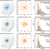 |
Fig. A.1 Nearest-neighbour comparisons for N = 200 points drawn from three centrally concentrated spherical profiles within R = 1.0. Top: Power law with slope p = −2. Middle: truncated Gaussian with σ = 0.25. Bottom: Plummer with scale radius a = 0.25. Each row shows the 3D NN graph (left), the 2D projection (centre), and the corresponding distributions of NN edge lengths (right). Projection shortens apparent separations and rewires most nodes to new, closer neighbours in 2D, with mean ratios ℓ3D/ℓ2D ~ 2.3–2.4, well above the geometric baseline 4/π ≃ 1.27. |
Finite spatial resolution systematically suppresses the projection ratio by blending small–scale structure. As a result, lower-SDR curves are shifted to smaller values of 𝒞 at all D, and the high–D asymptotic limit is recovered only for sufficiently large spatial dynamic range. Over the range D = 1.5–2.8 explored here, 𝒞 spans approximately 0.67–2.03 for SDR = 10, 1.43–2.38 for SDR = 50, and 1.72–2.43 in the high–resolution limit.
An additional feature is that, at the lowest fractal dimensions and spatial dynamic ranges, the dependence on D and SDR is not fully separable. For highly filamentary, strongly clustered distributions (low D), the intrinsic nearest–neighbour separations are dominated by compact substructures; when combined with poor spatial resolution (low SDR), beam blending efficiently merges these compact groupings, effectively erasing the small–scale clustering that distinguishes low–D morphologies. In this regime, 𝒞 is suppressed more strongly than would be expected from either low D or low SDR alone, indicating coupled behaviour between structure and resolution when both are extreme.
 |
Fig. B.1 Minimum spanning tree comparison for a uniform spherical distribution of N=200 points within radius R=1.0. Left: MST network constructed in 3D. Centre: MST built from the projected 2D positions (no rotation). Right: Distributions of MST edge lengths in 3D (blue) and 2D (orange), with medians (dashed lines) and kernel density estimates (KDEs) overplotted. The total MST length decreases from 38.4 (3D) to 16.1 (2D), corresponding to a mean ratio ⟨ℓ3D/ℓ2D⟩ ≃ 2.38, well above the geometric expectation (4/π) ≃ 1.27. Only ~25% of 3D edges are recovered in 2D (Jaccard similarity 0.14), indicating that projection not only foreshortens MST edges but also rewires the network topology—though less severely than for the NN graph (cf. Fig. 2). |
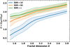 |
Fig. C.1 Projection ratio 𝒞 = ⟨ℓ3D⟩/⟨ℓ2D⟩ as a function of fractal dimension D for N = 200, evaluated at three spatial dynamic ranges: SDR = 10 (blue), SDR = 50 (orange), and the effectively infinite–resolution limit SDR → ∞ (green). Lower values of D correspond to more strongly clustered, filamentary (more “fractal”) structures, while higher values of D approach smoother, more space–filling morphologies. Solid lines show ensemble means, while shaded regions indicate the 1σ scatter across Monte Carlo realisations. The projection ratio increases monotonically with D and approaches an approximately asymptotic value at high D, with finite spatial resolution systematically reducing 𝒞 at all fractal dimensions. |
Overall, varying D primarily shifts the normalisation of 𝒞 and drives a monotonic increase that saturates for D ≳ 2.4 to 2.6, while the principal trends with N and SDR established in the main text remain unchanged. The coupled low–D, low–SDR regime simply delineates where finite resolution can erase the structural differences that otherwise distinguish filamentary morphologies.
All Tables
Fitted projection-correction factors 𝒞(N, SDR) from the empirical relation 𝒞(N, SDR) = 𝒞∞[1 − e−SDR/S0](N/100)β using 𝒞∞ = 1.94, S0 = 21.8, and β = 0.173.
All Figures
|
Fig. 1 Example of a 1.3 mm continuum image from the ASHES survey (Morii et al. 2023), overlaid with the NN graph (orange lines). The background colour scale and contours show the ALMA 12 m plus 7 m continuum emission, with contour levels at 3 × 2nσ (n = 0, 1, 2, . . .), where σ = 9.5 × 10⁻⁵ Jy beam−1 is the rms noise level. Detected core positions are marked by orange circles, and the scale bar in the lower left corresponds to 0.1 pc at the assumed distance 5.5 kpc. |
| In the text | |
|
Fig. 2 Nearest-neighbour comparisons for N = 200 points drawn from a uniform spherical distribution within R = 1.0. Top: NN graph constructed in 3D, where the blue connections are the 3D NNs (left); 2D projection, where the orange connections are the 2D NNs (Centre); and the corresponding distributions of NN edge lengths (right) highlighting the overall shortening in projection. Bottom: detailed breakdown. The left panel repeats the 2D overlay of 3D and 2D edges, while the right panels show the distributions of ℓ3D, ℓ2D for shared edges and the ratios ℓ3D/ℓ2D. Vertical dashed lines mark the medians, and KDEs are overplotted on the histograms. Together these panels illustrate how projection both compresses lengths and reassigns neighbours, with only the very shortest pairs surviving unchanged. |
| In the text | |
|
Fig. 3 Nearest-neighbour comparisons for uniformly sampled point distributions. Top: example realisation with N = 10 points drawn within a sphere of radius of R = 1.0. The NN graph constructed in 3D (left), its 2D projection obtained by dropping the line-of-sight coordinate (centre), and the corresponding edge-length distributions (right) illustrate how projection systematically shortens apparent separations and modifies the network connectivity even in a simple isotropic configuration. Bottom: results from the Monte Carlo ensembles (103 realisations each) for N = 5, 10, 20, and 50 showing stacked kernel density estimates of 3D (blue) and projected 2D (orange) NN edge lengths. The distributions converge at a stable median ratio as N increases, while stochastic fluctuations dominate at small values of N. |
| In the text | |
|
Fig. 4 Illustration of the impact of a finite SDR on NN statistics using a uniform distribution of N = 200 points within a sphere of radius R = 1.0. Left: intrinsic 3D NN graph. Centre: two-dimensional projection after applying a beam–blending step that merges points closer than one beam width, corresponding here to a SDR of SDR = FoV/FWHMbeam = 10. Circles mark the original 2D positions (open) and the resulting beam-blended centroids (filled). Right: distributions of NN edge lengths in 3D and 2D after blending. In this example, 135 of the 200 projected cores (67.5%) are merged into 65 effective groups, erasing all topological correspondence between the intrinsic and projected networks (J = 0.00, overlap fraction = 0). The typical 3D and 2D NN lengths become nearly equal (⟨ℓ3D⟩/⟨ℓ2D⟩ ≃ 1.0), as beam blending suppresses the shortest intrinsic separations that normally produce the geometric compression factor (4/π ≃ 1.27). This example illustrates that limited spatial resolution can strongly distort the apparent connectivity and scale distribution of dense cores even in an intrinsically uniform configuration. |
| In the text | |
|
Fig. 5 Nearest-neighbour graphs for a fractal distribution with N = 200 points, fractal dimension D = 1.6, and sub-division ndiv = 3, within R = 1.0. Each row shows the NN network in 3D (left), the projected NN network in 2D (centre), and the corresponding NN edge-length distributions (right). The three rows illustrate different viewing geometries: no rotation (top), rotation about the y-axis (β = 90°; middle), and rotation about the z-axis (γ = 90°; bottom). Projection systematically shortens the apparent NN separations and rewires connectivity, but the degree of overlap and compression depends on the line of sight, reflecting the anisotropic and clumpy structure of the fractal distribution. |
| In the text | |
|
Fig. 6 Nearest-neighbour projection ratio ℓ3D/ℓ2D versus sample size N for fractal ensembles. For each N, we averaged 100 realisations per configuration and then combined across nine fractal setups (D ∈ {1.7, 2.0, 2.5}, ndiv ∈ {2, 3, 4}) with jitter=True and prune=True. The solid curve shows the cross-configuration mean, and the dashed curves indicate ±1σ across configurations (not the run-to-run uncertainty). The dashed horizontal line marks the geometric fixed-pair baseline 4/π ≃ 1.27. Projection bias is present at all N, with ℓ3D/ℓ2D increasing sub-linearly with N and reaching ~2.0–2.3 by N = 200, depending on fractal parameters. A higher D (less clumpy) yields larger ratios at a fixed N, indicating that beyond geometric compression, crowding and neighbour reassignment drive additional shortening in projection. |
| In the text | |
|
Fig. 7 Nearest-neighbour projection ratio ⟨ℓ3D⟩/⟨ℓ2D⟩ as a function of SDR evaluated for fractal ensembles (D = 1.7–2.5, ndiv = 2–4) at a fixed value of N = 200. Points and shaded bands show the mean and ±1σ scatter across configurations. The projection bias increases rapidly up to SDR ~ 10–20, beyond which it asymptotically approaches the intrinsic structural limit (𝒞∞ ≈ 1.9–2.0). At a low SDR, beam blending dominates, merging close pairs and driving 𝒞 → 1, i.e. apparent isometry between 3D and 2D separations. |
| In the text | |
|
Fig. 8 Combined dependence of the projection distortion ratio 𝒞(N, SDR) = ⟨ℓ3D⟩/⟨ℓ2D⟩ on sample size N and SDR. Left: ensemble-averaged measurements from 1000 fractal realisations with D = 1.7–2.5 and ndiv = 2–4. Centre: best-fitting three-parameter model 𝒞∞[1 − e−SDR/S0](N/100)β. Right: fractional residuals (𝒞meas − 𝒞fit)/𝒞fit. The fitted parameters (𝒞∞ = 1.94, S0 = 21.8, β = 0.17) capture the joint behaviour across two orders of magnitude in both variables. The model converges to the geometric projection limit (𝒞 ≃ 1.3) for small well-resolved samples and to the beam-limited regime (𝒞 ≃ 1) when SDR ≲ 10. |
| In the text | |
|
Fig. 9 Effect of projection and resolution corrections on the distribution of NN separations in the ASHES survey (Morii et al. 2024). Top: Observed (projected) 2D separations. Middle: Separations corrected for projection bias using the Sample-size-dependent relation 𝒞(N) (Eq. (7)). Bottom: Separations corrected for both projection and finite angular resolution using 𝒞(N, SDR) (Eq. (6)). Dashed lines mark the median values in each panel. The uncorrected distribution peaks near 0.08 pc, increases to 0.12 pc after applying 𝒞(N), but returns to 0.07 pc when the finite dynamic range (SDR ~ 10–20, defined as clump radius to beam FWHM) is included. This demonstrates the competing influences of geometric projection, which lengthens apparent separations, and beam blending, which suppresses the shortest scales (note the caveats of applying this correction to observations in Sect. 5.3). |
| In the text | |
|
Fig. A.1 Nearest-neighbour comparisons for N = 200 points drawn from three centrally concentrated spherical profiles within R = 1.0. Top: Power law with slope p = −2. Middle: truncated Gaussian with σ = 0.25. Bottom: Plummer with scale radius a = 0.25. Each row shows the 3D NN graph (left), the 2D projection (centre), and the corresponding distributions of NN edge lengths (right). Projection shortens apparent separations and rewires most nodes to new, closer neighbours in 2D, with mean ratios ℓ3D/ℓ2D ~ 2.3–2.4, well above the geometric baseline 4/π ≃ 1.27. |
| In the text | |
|
Fig. B.1 Minimum spanning tree comparison for a uniform spherical distribution of N=200 points within radius R=1.0. Left: MST network constructed in 3D. Centre: MST built from the projected 2D positions (no rotation). Right: Distributions of MST edge lengths in 3D (blue) and 2D (orange), with medians (dashed lines) and kernel density estimates (KDEs) overplotted. The total MST length decreases from 38.4 (3D) to 16.1 (2D), corresponding to a mean ratio ⟨ℓ3D/ℓ2D⟩ ≃ 2.38, well above the geometric expectation (4/π) ≃ 1.27. Only ~25% of 3D edges are recovered in 2D (Jaccard similarity 0.14), indicating that projection not only foreshortens MST edges but also rewires the network topology—though less severely than for the NN graph (cf. Fig. 2). |
| In the text | |
|
Fig. C.1 Projection ratio 𝒞 = ⟨ℓ3D⟩/⟨ℓ2D⟩ as a function of fractal dimension D for N = 200, evaluated at three spatial dynamic ranges: SDR = 10 (blue), SDR = 50 (orange), and the effectively infinite–resolution limit SDR → ∞ (green). Lower values of D correspond to more strongly clustered, filamentary (more “fractal”) structures, while higher values of D approach smoother, more space–filling morphologies. Solid lines show ensemble means, while shaded regions indicate the 1σ scatter across Monte Carlo realisations. The projection ratio increases monotonically with D and approaches an approximately asymptotic value at high D, with finite spatial resolution systematically reducing 𝒞 at all fractal dimensions. |
| In the text | |
Current usage metrics show cumulative count of Article Views (full-text article views including HTML views, PDF and ePub downloads, according to the available data) and Abstracts Views on Vision4Press platform.
Data correspond to usage on the plateform after 2015. The current usage metrics is available 48-96 hours after online publication and is updated daily on week days.
Initial download of the metrics may take a while.