| Issue |
A&A
Volume 708, April 2026
|
|
|---|---|---|
| Article Number | A270 | |
| Number of page(s) | 28 | |
| Section | Interstellar and circumstellar matter | |
| DOI | https://doi.org/10.1051/0004-6361/202555954 | |
| Published online | 15 April 2026 | |
Characterization of Type Ibn Supernovae
1
DARK, Niels Bohr Institute, University of Copenhagen,
Jagtvej 155A,
2200
Copenhagen,
Denmark
2
Harvard-Smithsonian Center for Astrophysics,
60 Garden Street,
Cambridge,
MA
02138,
USA
3
Department of Astronomy and Astrophysics, University of California,
Santa Cruz,
CA
95064,
USA
4
OzGrav, School of Physics, The University of Melbourne,
VIC 3010,
Parkville,
Australia
5
The NSF AI Institute for Artificial Intelligence and Fundamental Interactions,
USA
6
Department of Physics, Massachusetts Institute of Technology,
Cambridge,
MA
02139,
USA
7
Institute for Astronomy, University of Hawaii,
2680 Woodlawn Drive,
Honolulu,
HI
96822,
USA
8
Department of Astronomy, University of Illinois at Urbana-Champaign,
1002 W. Green St.,
IL
61801,
USA
9
Center for Astrophysical Surveys, National Center for Supercomputing Applications,
Urbana,
IL
61801,
USA
10
NSF-Simons SkAI Institute,
875 N. Michigan Ave.,
Chicago,
IL
60611,
USA
11
Department of Physics and Astronomy, The Johns Hopkins University,
Baltimore,
MD
21218,
USA
12
Astrophysics Research Center of the Open University (ARCO), The Open University of Israel,
Ra’anana,
4353701
Israel
13
Department of Natural Sciences, The Open University of Israel,
Ra’anana
4353701,
Israel
14
Astrophysics Research Centre, School of Mathematics and Physics, Queen’s University Belfast,
Belfast
BT7 1NN,
UK
15
Hubble Fellow, Department of Astronomy and Astrophysics, California Institute of Technology,
Pasadena,
CA
91125,
USA
16
Institute for Astronomy, University of Hawaii,
640 N.‘Aohoku Pl.,
Hilo,
HI
96720,
USA
17
Center for Interdisciplinary Exploration and Research in Astrophysics (CIERA) and Department of Physics and Astronomy, Northwestern University,
Evanston,
IL
60208,
USA
18
Department of Physics, Fisk University,
1000 17th Avenue N.
Nashville,
TN
37208,
USA
19
Department of Physics, Lancaster University,
Lancaster,
LA1 4YB,
UK
20
Oskar Klein Centre, Department of Astronomy, Stockholm University, AlbaNova,
106 91
Stockholm,
Sweden
21
INAF, Osservatorio Astronomico di Capodimonte,
salita Moiariello 16,
80131
Naples,
Italy
22
Observatories of the Carnegie Institute for Science,
813 Santa Barbara St.,
Pasadena,
CA
91101,
USA
23
Space Telescope Science Institute,
Baltimore,
MD
21218,
USA
24
National Astronomical Research Institute of Thailand,
260 Moo 4, Donkaew, Maerim,
Chiang Mai
50180,
Thailand
★ Corresponding author: This email address is being protected from spambots. You need JavaScript enabled to view it.
Received:
15
June
2025
Accepted:
17
February
2026
Abstract
Context. Type Ibn supernovae (SNe) are characterized by narrow helium (He I) lines from photons produced by the unshocked circumstellar material (CSM). About 80 SNe Ibn have been discovered to date and only a handful of them have extensive observational records. Thus, many open questions remain regarding the progenitor system and the origin of CSM.
Aims. Here, we investigate potential correlations between the spectral features of the prominent He I λ5876 Å line and the optical and X-ray light curve properties of Type Ibn SNe (SNe Ibn).
Methods. We compiled the largest sample of 61 SNe Ibn to date, of which 24 SNe have photometric and spectroscopic data available from the Young Supernova Experiment and 37 SNe benefit from archival datasets. We fit 24 SNe Ibn with sufficient photometric coverage (B to z bands) using semi-analytical models from MOSFiT.
Results. We demonstrate that the light curves of SNe Ibn are more diverse than previous analyses suggest, with absolute r-band peak magnitudes (rmax) of −19.4 ± 0.6 mag, along with rise (from −10 days to peak, γ−10) and decay rates (from peak to +10 days; γ+10) of −0.08 ± 0.06 and 0.08 ± 0.03 mag/day, respectively. We find that the majority of SNe Ibn in the subsample are consistent with a low-energy explosion (< 1051 erg) of a star with a compact envelope surrounded by ~0.1 M⊙ of helium-rich CSM. The inferred ejecta masses are small (Mej ~ 1 M⊙) and expand with a velocity of ~5000 km/s. Our spectroscopic analysis shows that the mean velocity of the narrow component of the He I lines, associated with the CSM, peaks at ~1100 km/s.
Conclusions. The mean CSM and ejecta masses inferred for a subsample of SNe Ibn indicate that their progenitors are not massive (~10 M⊙) single stars at the moment of explosion; rather, they are likely to be binary systems. This finding is in agreement with detections of potential companion stars of SNe Ibn progenitors and inferred CSM properties from stellar evolution models.
Key words: circumstellar matter / supernovae: general / stars: winds, outflows / stars: Wolf–Rayet
© The Authors 2026
 Open Access article, published by EDP Sciences, under the terms of the Creative Commons Attribution License (https://creativecommons.org/licenses/by/4.0), which permits unrestricted use, distribution, and reproduction in any medium, provided the original work is properly cited.
This article is published in open access under the Subscribe to Open model. This email address is being protected from spambots. You need JavaScript enabled to view it. to support open access publication.
1 Introduction
The majority of massive stars (M* ≳ 8M⊙) end their lives as core-collapse supernovae (CCSNe). The photometric and spectroscopic characteristics of these explosions reflect differences in the physical properties of their progenitors, power sources, and local environments. In studies of these properties, CCSNe are further classified into various types and subtypes. The two primary classes are distinguished by the absence (Type I) or presence (Type II) of hydrogen in their spectra (Filippenko 1997, and references therein). Further divisions into subtypes (e.g., Ib, Ic, IIn) are based on photometric and spectroscopic features indicating the presence or absence of specific elements (e.g., helium), as well as evidence of circumstellar material (CSM) and its composition or interaction with the ejecta. The CSM is typically produced by the progenitor system prior to explosion, often through complex mass-loss processes (Smith 2014, and references therein). SNe interacting with a surrounding CSM gives rise to narrow (≲ 3000 km/s) emission and absorption lines of elements present in the slow-moving material (Dessart 2024, and references therein). For example, Type Ibn SNe (Pastorello et al. 2007; Foley et al. 2007) are embedded in a He-rich CSM and exhibit strong, narrow He I lines in the spectra.
In this work, we focus on SNe Ibn. These SNe are rare and their volumetric rate indicates that they only make up about 1–2% of all CCSNe (Maeda & Moriya 2022; Warwick et al. 2024). Typically, SNe Ibn are characterized by rapidly evolving light curves, with rise times of about 10 days. Past peak brightness, their optical magnitude declines by about 0.1 mag/day (Hosseinzadeh et al. 2017; Ho et al. 2021). Outbursts preceding the SN explosion have been observed in some SNe Ibn, such as 2006jc (Pastorello et al. 2007), 2019uo (Gangopadhyay et al. 2020; Strotjohann et al. 2021), and 2023fyq (Brennan et al. 2024; Dong et al. 2024). Around peak brightness, the spectra of SNe Ibn exhibit relatively narrow (v ~ 3000 km/s) He I lines on top of a blue (T ≳ 10 000 K) continuum (Pastorello et al. 2016). Continuous interactions between the SN shock, ejecta, and the CSM produce intermediate velocity components (v ~ 4000 km/s) of the He I lines (Pastorello et al. 2015b). Broad (v ~ 10 000 km/s) spectral features (if present) are likely associated with emission coming from the SN ejecta (Fraser 2020). About one month from peak brightness, the spectra of SNe Ibn are characterized by emission lines of calcium, magnesium, and a blue pseudo-continuum at about 5500 Å due to the emission of a forest of iron lines (Dessart et al. 2022). Several SNe Ibn such as SN 2019uo (Gangopadhyay et al. 2020), SN 2019wep (Gangopadhyay et al. 2022), and SN 2023emq (Pursiainen et al. 2023) show strong emission of highly ionized, narrow carbon lines at early phases. Such lines are characteristic of Type Icn SNe (Gal-Yam et al. 2022; Fraser et al. 2021; Davis et al. 2023b). The presence of carbon lines in the early spectra of a growing number of SNe Ibn may indicate a continuum between the Ibn and Icn types (Pursiainen et al. 2023).
The nature of the progenitor system of SNe Ibn remains elusive. Several suggestions of progenitor systems that can account for the observed characteristics have been put forward. For the prototypical example of the Ibn class, SN 2006jc, deep preexplosion imaging revealed a precursor outburst, detected two years before the SN explosion. This evidence trongly supports a scenario involving a Wolf–Rayet (WR) progenitor star undergoing episodic mass loss (Pastorello et al. 2008b). This scenario is also supported by the observed photometric homogeneity in a sample of SNe Ibn (Hosseinzadeh et al. 2017) and the ejecta masses (Mej ≃ 10 M⊙) estimated by light curve modeling (Karamehmetoglu et al. 2017; Gangopadhyay et al. 2020; Kool et al. 2021; Wang et al. 2021). Alternatively, a binary interaction between two lower mass stars, such as an accreting helium star (M* ≲ 5 M⊙) and a compact object (e.g., a neutron star) has also been proposed for SNe Ibn 2006jc and 2019uo (Tsuna et al. 2024a). A similar scenario invoking an unstable mass transfer and merging of the helium and neutron star was proposed for SN 2023fyq based on the brightness and timescale of the observed precursor emission (Dong et al. 2024; Tsuna et al. 2024b). Furthermore, late-time photometric observations at the location of SN 2006jc revealed the presence of a potential surviving companion star (Maund et al. 2016; Sun et al. 2020). Theoretical modeling suggests that such systems can create massive CSM shells through multiple mass transfer episodes (Wu & Fuller 2022). In stellar evolution models, it is easier to obtain He-rich SN ejecta masses of ~4 M⊙ from binary systems than from single stars (Dessart et al. 2022; Takei et al. 2024). To date, only two sample studies of SNe Ibn exist, namely, by Pastorello et al. (P16; 2016) and Hosseinzadeh et al. (H17; 2017), which primarily focus on the observational properties. More than 40 SNe Ibn have been discovered since the most recent study (H17), some of which are studied in detail (e.g., Karamehmetoglu et al. 2017; Ho et al. 2021; Karamehmetoglu et al. 2021; Kool et al. 2021; Pellegrino et al. 2022b; Ben-Ami et al. 2023). In this work, we present the photometric and spectroscopic observations of 24 SNe Ibn enabled by the Young Supernova Experiment (YSE; Jones et al. 2021a; Aleo et al. 2022).
The ongoing transient YSE survey uses a 7% time allocation of the Panoramic Survey Telescopes and Rapid Response System (Pan-STARRS; Chambers et al. 2016) of PS1 & PS2 to scan ~750 deg2 of the sky, with an approximate three-day cadence to a depth of gri ≈ 21.5 mag and z ≈ 20.5 mag (Aleo et al. 2022). Hereafter, these 24 SNe Ibn are referred to as the F25 sample (Fig. 1). In addition, 15 out of the 24 SNe in the F25 sample have X-ray observations (i.e., the X-RAY sample), which we analyze in this work.
We complemented the F25 sample with archival photometric and spectroscopic data of 37 SNe Ibn, referred to as the “literature” (Lit) sample (see Fig. 1, Tables D.8 and Table D.7). Overall, we studied the photometric and spectroscopic properties of 61 SNe Ibn (F25+Lit), the largest sample to date assembled for this class. From the combined sample (F25+Lit), we selected 24 Type Ibn SNe with well-sampled light curves (hereafter referred to as the MOSFiT sample; see Fig. 1). These SNe were modeled using MOSFiT with a self-consistent fitting approach. Such an approach is essential for exploring the physical parameters associated with the CSM and the explosion properties of SNe Ibn at the population level, as light curve modeling is sensitive to the chosen model implementation, the set of free parameters, and the prior distributions used in the fits. We also present the analysis of prominent He I emission lines in the spectra of 59 out of the 61 SNe Ibn. We measured the velocities of these lines for 43 SNe with spectra taken from the Weizmann Interactive Supernova Data Repository (WISeREP)1 and this work (see Table D.7). Additionally, we include the measurements of He I emission line velocities of 16 SNe Ibn presented in P16, H17, Gangopadhyay et al. (2022), and Wang et al. (2024b).
The paper is organized as follows. Section 2 describes the acquisition and reduction of photometric and spectroscopic data of the 24 YSE-observed SNe Ibn (F25 sample), which are presented for the first time in this work. Section 3 outlines the methods used to estimate the photometric properties, such as the peak magnitudes and color evolution. The light curve modeling approach of the MOSFiT sample is detailed in Section 4. Section 5 discusses the X-ray analysis of 15 YSE-observed SNe Ibn in the X-RAY sample. Section 6 presents the analysis method and results of the decomposition of the He I λ5876 Å profiles of 59 SNe Ibn from our total (F25+Lit) sample. In Section 7, we discuss the results and present our conclusions in Section 8.
 |
Fig. 1 Visualization of the four different SN Ibn samples (F25, X-RAY, MOSFiT, and Lit) analyzed in this work, with the individual member SN labeled. For details, see Tables D.8 and Table D.7b. |
2 The F25 sample
The F25 sample (see Fig. 1) of SNe Ibn consists of objects that have either been observed by the YSE collaboration between the years 2020 and 2023 or those that did not have well-sampled light curves at the beginning of 2024. Here, well-sampled light curves refer to photometric data obtained at a 1–4 day cadence between −3 days to +50 days relative to peak brightness and in at least three different filter bands. In total, 24 SNe Ibn fulfill these criteria.
There are 15 SNe in the F25 sample with photometric and/or spectroscopic follow-up observations obtained with resources by the YSE collaboration. Two SNe in this group, SN 2021iyt and SN 2021zfx, are YSE discoveries. Seven of the F25 SNe have extensive photometric and spectroscopic data coverage. These seven YSE Ibn SNe are SN 2020nxt (Wang et al. 2024a), SN 2020able, SN 2021iyt, SN 2021zfx, SN 2022gzg, SN 2022qhy, and SN 2023iuc. The eight remaining SNe, SN 2022eux, SN 2022ihx, SN 2022pda, SN 2023emq (Pursiainen et al. 2023), SN 2023qre, SN 2023rau, SN 2023xgo (Gangopadhyay et al. 2025), and SN 2023abbd have sporadic data coverage obtained by YSE. Nine SNe of the F25 sample are not YSE-related. For five of these SNe Ibn (SN 2020taz, SN 2021wvg, SN 2023ubp, SN 2023utc, and SN 2023vwh), we obtained the photometric data from the Pan-STARRS Survey for Transients (PSST; Chambers et al. 2016). Data for two more SNe Ibn, SN 2018jmt, and SN 2022ablq are from Wang et al. (2024b) and Pellegrino et al. (2024), respectively. Additionally, we include two SNe Ibn from public surveys (SN 2019lsm and SN 2022acm) with as-yet-unpublished data that fulfill our selection criterion. For this work, we reprocessed all publicly available photometric data. Details of the photometric data of the F25 sample and their reprocessing are given in Sect. 2.1. All the data used in our analysis have been published alongside the paper.
2.1 Photometric data
We describe the data acquisition and reduction of photometric data of the SNe in the F25 sample obtained by eight different facilities below. The photometric data are reported in Table D.1.
2.1.1 Optical and UV
For 12 SNe Ibn in our sample, the optical photometric data were obtained with the Pan-STARRS telescopes (PS1 and PS2) located at Haleakala Observatory, Hawaii, USA (Chambers et al. 2016). Data were acquired in the same survey mode as employed by YSE (Jones et al. 2021a; Aleo et al. 2022) and accessed through YSE-PZ (Coulter et al. 2023) and the Pan-STARRS Survey for Transients (PSST; Huber et al. 2015). For SNe 2020nxt (Wang et al. 2024a), 2020able (Aleo et al. 2022), 2021iyt, 2021zfx, 2022gzg, 2022qhy, and 2023iuc, YSE obtained optical photometry in griz bands. PSST SNe 2021wvg, 2023ubp, 2023utc, 2023vwh, and 2023abbd were observed in wgrizy bands. All images from Pan-STARRS were reduced following the procedure detailed in Aleo et al. (2022). Basic data processing was performed by the PS1 Image Processing pipeline (Magnier et al. 2020). Template images were taken from the PS1 3π sky survey (Chambers et al. 2016). Template convolution and differencing photometry were performed using the Photpipe (Rest et al. 2005; Rest et al. 2014) pipeline. The difference fluxes are calibrated using nightly zero-points calculated from photometric standard stars from the PS1 3π sky survey.
Fourteen SNe Ibn also have ZTF g- and r-band photometry included in this work: SNe 20191sm, 2020taz, 2021wvg, 2022acm, 2022gzg, 2022ihx, 2022pda, 2023emq, 2023iuc, 2023rau, 2023ubp, 2023utc, 2023vwh, and 2023xgo. We retrieved all available public photometric data of these SNe from the Lasair broker (Smith et al. 2019) and no further processing was performed.
SN 2023rau was observed in griz bands with the 1-m Lulin Optical Telescope located at Lulin Observatory, Taiwan. All images were processed using bias and flat-field calibration frames following standard methods. We then performed photometry and pixel-level calibration in Photpipe following methods similar to those described above for the Pan-STARRS photometry.
Fifteen SNe were observed with the Ultraviolet and Optical Telescope (UVOT; Roming et al. 2005) on the Neil Gehrels Swift Observatory, in the V, B, U, UVW1, UVM2, UVW2 bands. SNe 2020nxt, 2022eux, 2022ihx, 2022qhy, 2022ablq, 2023emq, 2023qre, and 2023xgo were observed in all six UVOT bands. SNe 2020able, 2021iyt, and 2023iuc lack only V band and SN 2022pda lacks V and B band observations. We used the uvotsource tool from the HEASoft v6.26 package to perform aperture photometry within a 3″ aperture centered on all UVOT SNe. We subtracted the background of our science images using observations of the site of the SNe once these have faded. We report the measured magnitudes in each UVOT band for the observed SNe Ibn at a > 3σ level.
SN 2023xgo was observed in g′, r′, i′, and z′ bands with the Thacher 0.7-m telescope in Ojai, California (Swift et al. 2022). Through Photpipe, we performed pixel-level calibration using bias and flat-field frames obtained in the same night and with the instrumental configuration as our science frames. We then performed PSF photometry using DoPhot and calibrated the resulting griz magnitudes from the Pan-STARRS1 catalog (Flewelling et al. 2020).
SNe 2022qhy, 2023emq, 2023qre, and 2023rau were observed in uBVgri bands by the Direct 4k×4k camera on the 1-m Henrietta Swope telescope located at Las Campanas Observatory, Chile. For details on the complete reduction process, we refer to the description in Kilpatrick et al. (2018).
Fifteen SNe Ibn were observed by ATLAS (Tonry et al. 2018) in either orange (o) or cyan (c) bands of which SNe 2020nxt, 2020able, 2021iyt, 2022gzg, 2023emq, and 2023xgo were observed in both bands. SNe 2021zfx, 2022eux, 2022ihx, 2022pda, 2023rau, 2023ubp, 2023utc, 2023vwh, and 2023abbd were only observed in o band. Following the procedure described in Rest et al. (2024) and Farias et al. (2024), we extracted photometry at eight different circular regions surrounding each of these SNe at each epoch and in each band. If the flux measurements in these regions were not consistent with zero, then the epoch was flagged and not considered as a detection. The final product is a one-day binned light curve calculated as a 3σ-cut weighted mean in each band.
For five SNe Ibn, we obtained photometry with the Sinistro cameras on the Las Cumbres Observatory Global Telescope (LCOCT) 1-m telescope network (Brown et al. 2013). We adopted the LCOGT data for SN 2020nxt, published in Wang et al. (2024a), in this study. LCOGT unpublished photometric observations of SNe 2022ihx (gp, rp, ip), 2022pda (U, V, gp, rp, ip), and 2023iuc (gp, rp, ip) are presented in this work. Additionally, we also reprocessed the LCO B, V, gp, rp, ip, z images for SN 2018jmt (Wang et al. 2024b). We used the LCO BANZAI pipeline (McCully et al. 2018) to preprocess the imaging data (bias and flat-fielding). The image subtraction was done using Photpipe pipeline (Rest et al. 2005; Jones et al. 2021a). Thereafter, we performed PSF photometry using DoPhot (Schechter et al. 1993). To obtain the final magnitudes, we calibrated the data using u-band SDSS (Alam et al. 2015) together with griz Pan-STARRS1 photometric standards observed in the vicinity of the SNe.
2.1.2 X-ray
The X-RAY sample consists of 15 SNe Ibn (SNe 20191sm, 2020nxt, 2020able, 2021iyt, 2021zfx, 2022eux, 2022ihx, 2022pda, 2022qhy, 2022ablq, 2023emq, 2023iuc, 2023qre, 2023rau, and 2023xgo) which were observed with the Swift X-ray Telescope (XRT, Burrows et al. 2005) in photon counting mode (see Fig.1). To place constraints on the presence of any X-ray emission, we reprocessed all XRT observations from level one data using the package xrtpipeline version 0.13.7 and applied the standard filter and screening criteria,2 along with the most recent calibration files. For the vast majority of SNe in the X-RAY sample, we used a source region with a radius of 30″ centered on the position of the SN and a source-free background region to constrain the X-ray emission. For the SNe located close to complex regions (i.e., near the center of their host or a bright X-ray region), we used a source region with a radius of 20″(SN 2020able), 15″(SN 2020nxt, 2022ihx, 2022pda, 2023xgo), or 10″(SN 2022qhy, 2022ablq). To increase the signal-to-noise ratio (S/N), we stacked these individual observations together using xselect version 2.5b to either place the strongest constraint on the X-ray emission arising from the SN or in multiple time bins to obtain an X-ray light curve.
With the exception of SN 2020nxt, SN 2022qhy, SN 2022ablq, and SN 2023emq, we find no significant X-ray emission associated with individual nor the stacked observations of the SN. However, the emission towards SN 2020nxt and SN 2022qhy are very close to the center of their host galaxies, so it is likely that the detected emission is not entirely from the SNe. For the observations that we did not detect any X-ray emission for, we derived 3σ upper limits to the count rate in the 0.3–10.0 keV energy range. All count rates were corrected for the size of the aperture. To convert the 0.3–10.0 keV count rate into an unabsorbed X-ray flux (and luminosity) in the same energy band, we assumed an absorbed thermal bremsstrahlung model with a temperature of 2.3 keV, similar to the value assumed by Pellegrino et al. (2024). With the exception of SN 2022ablq, whose column density was taken from Pellegrino et al. (2024), all SNe have had their column densities derived using the H I maps published in HI4PI Collaboration (2016).
2.2 Optical spectroscopic data
Overall, 74 spectra of the SNe Ibn in F25 sample were obtained from multiple observing facilities through programs within the YSE collaboration. Additionally, 23 archival spectra were taken from WISeREP. The archival spectra from WISeREP are classification spectra from different collaborations, such as Spectroscopic Classification of Astronomical Transients collaboration (SCAT; Tucker et al. 2022), which were taken using the SuperNova Integral-Field Spectrograph (SNIFS; Lantz et al. 2004) and the Global Supernova Project collaboration using the FLOYDS-N/S and Goodman spectrograph. A log of the spectroscopic observations is presented in Table D.2. Furthermore, SNe 2023iuc, 2023qre, and 2023rau were observed with the Wide Field Spectrograph (WiFeS), mounted at the Australian National University (ANU) 2.3-m telescope located at the Siding Spring Observatory (Dopita et al. 2007). WiFeS is an integralfield spectrograph with a field-of-view of 38 × 25 arcsec. Each spectrum was taken in ‘nod & shuffle’ mode using the R = 3000 grating, which covers 3200–9800 Årange. Each observation was reduced using PyWiFeS (Childress et al. 2014), with the sky subtraction carried out using a 2D sky spectrum that was taken during the observations (Carr et al. 2024).
SNe 2020nxt, 2020able, 2021iyt, 2021zfx, 2022ihx, 2022pda, 2023emq, 2023qre, 2023rau, and 2023xgo were observed with the Kast dual-beam spectrograph (Miller & Stone 1993) on the Shane 3-m telescope at the Lick Observatory. To reduce the Kast spectra, we used the UCSC Spectral Pipeline3 (Siebert et al. 2019), a custom data-reduction pipeline based on procedures outlined by Foley et al. (2003), Silverman et al. (2012), and in the references given therein. The two-dimensional (2D) spectra were bias-corrected, flat-field corrected, adjusted for varying gains across different chips and amplifiers, and trimmed. A cosmic-ray rejection was applied using the pzapspec algorithm to individual frames. Multiple frames were then combined with appropriate masking. One-dimensional (1D) spectra were extracted using the optimal algorithm (Horne 1986). The spectra were wavelength-calibrated using internal comparison-lamp spectra with linear shifts applied by cross-correlating the observed night-sky lines in each spectrum to a master night-sky spectrum. Flux calibration was performed using standard stars at similar airmass to the science exposures, with “blue” (hot subdwarfs; i.e., sdO) and “red” (low-metallicity G/F) standard stars. We corrected for atmospheric extinction. By fitting the continuum of the flux-calibrated standard stars, we determined the telluric absorption in those stars and apply a correction, adopting the relative airmass between the standard star and the science image to determine the relative strength of the absorption. We allowed for slight shifts in the telluric A and B bands, which we determined through cross-correlation. For dual-beam spectrographs, we combined the sides by scaling one spectrum to match the flux of the other in the overlap region and used their error spectra to correctly weight the spectra when combined. More details of this process are discussed in the literature (Foley et al. 2003; Silverman et al. 2012; Siebert et al. 2019).
SNe 2021iyt, 2023emq, 2023qre, and 2023rau were observed with the Goodman spectrograph (Clemens et al. 2004) on the NOIRLab 4.1-m Southern Astrophysical Research (SOAR) telescope at Cerro Pachón, Chile. We used the UCSC Spectral Pipeline to reduce the Goodman spectra as described above for Kast. SNe 2021iyt, 2022pda, 2022ihx, 2023emq, 2023iuc, 2023rau, and 2023xgo were observed with the Alhambra Faint Object Spectrograph and Camera (ALFOSC) on the 2.56-m Nordic Optical Telescope (NOT). All ALFOSC spectra were obtained using a 1.0″ slit with grisms #4. We used standard routines within IRAF4 and PYRAF5 to reduce, extract, wavelength-calibrate, and flux-calibrate the spectra. SNe 2020nxt, 2020able, 2021iyt, and 2022gzg were observed with the Low Resolution Imaging Spectrometer (LRIS; Oke et al. 1995; Rockosi et al. 2010) mounted on the Keck I telescope, Hawaii. We used the UCSC Spectral Pipeline to reduce the LRIS spectra as described above for Kast and Goodman. SNe 2021zfx, 2022gzg and 2023abbd were observed with Gemini Multi-Object Spectrograph (GMOS) at Gemini South Observatory through Large and Long Program LP-204 (PI: W. Jacobson-Galán JacobsonGalán 2025). For all of these spectroscopic observations, a standard CCD processing, spectrum extraction, and flux calibration were carried out with the DRAGONS pipeline (Labrie et al. 2019).
3 Photometric analysis
We present a consistent approach to analyze the light curves of all SNe Ibn in the F25+Lit sample (see Sect. 2; Fig. 1 and Table D.8). Our analysis aims to identify correlations between the photometric properties within the Type Ibn class.
3.1 Data preprocessing
The majority of the 61 SNe in the F25+Lit sample have light curves in multiple bands at a high cadence (~3 days). However, there are periods of missing data in different bands, usually as a result of unfavorable weather. To consistently analyze the light curves of the SNe in each band, we constructed uniformly sampled light curves (with a one-day cadence) from the photometric data using a Gaussian process (GP; Rasmussen & Williams 2005) with a Matern32 kernel6 implemented in george (Ambikasaran et al. 2015). The GP interpolation was performed on the flux in each band versus time space, rather than in magnitude space, to incorporate low-S/N observations; nevertheless, this approach allowed us to constrain the shape of the GP at all phases. We optimize the length scale of the kernel of the GP by maximizing the log-likelihood of the modeled light curve and the data using scipy optimize (Virtanen et al. 2020). Thereafter, we masked the interpolated light curves to ensure the S/N of each data point exceeded 3.
3.2 Peak magnitude
We chose the interpolated r-bands (e.g., ZTF-r, ATLAS-o, and/or PS1-r, depending on availability) to estimate the time of the peak (tmax) and the peak r-band magnitude in a given r-band (rmax) of the 61 SNe Ibn. We did not utilize the maximum of the interpolated light curve for the peak magnitude given that simple stationary kernels are prone to cause the interpolated posterior mean of the light curve to being undersmooth or oversmooth, while also underestimating the error on the time of peak (Stevance & Lee 2023). Instead, we used a Markov chain Monte Carlo (MCMC) approach, as implemented in the emcee7 (Foreman-Mackey et al. 2013) Python package to fit a second order polynomial to the interpolated r-band light curves between ±10 days of the peak. We used 100 walkers, 10 000 iterations, and a burn-in period of 1000 steps (see Table D.8). In total, 13 of the 61 SNe lack of photometric data around the peak and, thus, the peak time and magnitude cannot be estimated with this method. These 13 SNe are: SNe 2000er, 2002ao, 2005la, 2006jc, 2011hw, LSQ12btw, 2014bk, ASASSN-14ms, 2015G, 2019wep, 2020bqj, 2022qhy, and 2023abbd. For SNe 2000er, 2002ao, 2005la, 2006jc, 2011hw, LSQ12btw, 2014bk, ASASSN-14 ms, and, 2015 G, we retrieved the values reported in Table 4 from H17. The peak dates and magnitudes of SNe 2019wep and 2020bqj were obtained from Gangopadhyay et al. (2022) and Kool et al. (2021), respectively. For SNe 2022qhy and 2023abbd in the F25 sample, we assumed the peak time and peak magnitude from the first detection in V and o bands, respectively, as these are closest available photometric bands to r for these objects.
3.3 Dust extinction
For all SNe in the F25 sample, the Galactic reddening E(B − V)MW is the mean color excess along the line of sight towards each SN which is taken from the dust maps of Schlafly & Finkbeiner (2011). The values of E(B − V)MW are reported in Table D.3. The Galactic extinction in different bands was obtained using the dust extinction law of Fitzpatrick (2004) through the dust_extinction (Gordon 2024) package assuming RV = 3.1. We applied the extinction correction after preprocessing the light curves (Sect. 3.1.)
For all SNe in F25 that do not have reported host extinction in previous studies, we followed a similar approach to Shivvers et al. (2016) to estimate E(B − V)host. We fit a blackbody (BB) function modified to account for dust extinction to the spectral energy distribution (SED) at the time of the r-band maximum. From the interpolated light curves at tmax, we constructed the SED of each SN by requiring at least three filters with effective wavelengths between 4500 Å and 9000 Å (i.e., B to z bands). We find 16 SNe that fulfill our “three-filter” criterion. We explored the posterior distributions of three free parameters TBB, RBB and E(B − V)host in our SED BB fitting. To do so, we used the nested sampler dynesty (Speagle 2020), assuming uniform prior distributions on the three parameters.
The results of this analysis for SNe 2020able, 2022ihx, 2023iuc and 2023xgo are shown in Fig. A.1. For SNe 2018jmt and 2023emq, the absence of Na I D lines suggests that E(B − V)host is negligible (Wang et al. 2024b; Pursiainen et al. 2023). For these SNe, we have E(B − V)host ≲ 0.1 mag. In contrast, SN 2022ablq appears significantly extinguished by dust along the line of sight towards the SN in the host galaxy. Pellegrino et al. (2024) estimate E(B − V)host = 0.18 ± 0.1 mag, whereas we obtained E(B − V)host = 0.35 mag, with an uncertainty of ≈ 0.1 mag, within 1σ from the value reported in the previous work. Recently, Wang et al. (2025) estimated E(B − V)host ≲ 0.09 mag, E(B − V)host ≲ 0.03 mag, and E(B − V)host ≲ 0.26 mag, for SNe 2020nxt, 2020taz, and 2023utc, respectively. These estimates were based on empirical relations between the equivalent width (EW) of the narrow sodium (Na) absorption lines, Na I D λλ5890, 5896 Å, and E(B − V) (Turatto et al. 2003; Poznanski et al. 2012). However, Wang et al. (2025) assumed negligible host extinction based on host galaxy properties and the location of the SNe in their hosts. Similarly, using the EW-E (B − V) relation from Poznanski et al. (2012), Gangopadhyay et al. (2025) estimated E(B − V)host ≈ 0.01 mag. Though, the color excess noticed in both SN 2023xgo from Gangopadhyay et al. (2025) and SN 2020taz from Wang et al. (2025) are smaller than those obtained with our method, which are ![Mathematical equation: $\[0.09_{-0.05}^{+0.05}\]$](/articles/aa/full_html/2026/04/aa55954-25/aa55954-25-eq1.png) mag and
mag and ![Mathematical equation: $\[0.09_{-0.06}^{+0.06}\]$](/articles/aa/full_html/2026/04/aa55954-25/aa55954-25-eq2.png) mag, respectively. The discrepancies between both methods can either be due to a poorly sampled SED, to the approximation of the SN SED by a modified BB, or to low-resolution spectra. As also pointed out by Wang et al. (2025); Byrne et al. (2023), the empirical relations between color excess and EWs are not adequate for estimating the host extinction of SNe Ibn, since the EWs of Na I D lines are likely affected by the photoionization of the CSM. Thus, the values of the E(B − V)host obtained with our method might differ from, for example, a potential extinction estimation using Na I D lines (see Sect. A for further discussion on the extinction estimation of SNe 20191sm, 2020able and 2021wvg). For eight SNe (for which no independent extinction estimates are available and for which the SEDs at tmax cannot be constructed due to lack of data), we assumed zero extinction associated with the host galaxies. These SNe are: 2020nxt, 2021zfx, 2022qhy, 2023qre, 2023ubp, 2023utc, 2023vwh, and 2023abbd. For SN 2023qre, this assumption is further confirmed by the inferred host extinction through light curve modeling (Sect. 4). For all SNe in the Lit sample, we took the total (MW + host) extinction estimates from their respective references, as shown in Table D.8.
mag, respectively. The discrepancies between both methods can either be due to a poorly sampled SED, to the approximation of the SN SED by a modified BB, or to low-resolution spectra. As also pointed out by Wang et al. (2025); Byrne et al. (2023), the empirical relations between color excess and EWs are not adequate for estimating the host extinction of SNe Ibn, since the EWs of Na I D lines are likely affected by the photoionization of the CSM. Thus, the values of the E(B − V)host obtained with our method might differ from, for example, a potential extinction estimation using Na I D lines (see Sect. A for further discussion on the extinction estimation of SNe 20191sm, 2020able and 2021wvg). For eight SNe (for which no independent extinction estimates are available and for which the SEDs at tmax cannot be constructed due to lack of data), we assumed zero extinction associated with the host galaxies. These SNe are: 2020nxt, 2021zfx, 2022qhy, 2023qre, 2023ubp, 2023utc, 2023vwh, and 2023abbd. For SN 2023qre, this assumption is further confirmed by the inferred host extinction through light curve modeling (Sect. 4). For all SNe in the Lit sample, we took the total (MW + host) extinction estimates from their respective references, as shown in Table D.8.
3.4 Color evolution
Figure 2 shows the evolution of the interpolated B − V and g − r light curves without any corrections for host or Galactic extinction. It is evident that neither SNe Ibn nor SNe Icn form a homogeneous group, as there is a spread of approximately one magnitude in the color curves throughout the SN evolution. We note that the “Icn/Ibn” group refers to SNe whose classification spectra have been reported to resemble that of SN 2023emq (see Table D.3). This similarity is based on the presence of a spectral feature at 5696 Å, which is associated with the C III emission line. The SNe classified as Icn/Ibn SNe are SN 2023emq, 2023qre, 2023rau, and 2023xgo (this work). This sample of SNe Icn/Ibn do not form a homogeneous group either.
Figure 2 illustrates that the evolution of the B − V and g − r color curves is too diverse to be a reliable indicator of extinction. Therefore, it is challenging to create color templates for SNe Ibn that would resemble those created for stripped-envelope SNe (Stritzinger et al. 2018).
 |
Fig. 2 Interpolated B − V (top) and g − r (bottom) curves for the 24 SNe Ibn from F25 (magenta filled circles), the Icn/Ibn (2023emq-like: yellow filled circles) and the color curves (±1σ) of the Lit sample (blue regions). The color curves (±1σ) of five SNe Icn are included for comparison (red regions). The photometric data of the SNe Icn were retrieved from Gal-Yam et al. (2022); Perley et al. (2022); Fraser et al. (2021); Pellegrino et al. (2022a); Davis et al. (2023b). |
3.5 Absolute R/r-band light curve
We compute the extinction-corrected, absolute magnitudes of the R/r-band light curves for all 61 SNe Ibn in the F25+Lit sample shown in Fig. 3. To do so, we derive the distance modulus for all SNe assuming ΛCDM cosmology with H0 = 67.8 km s−1 Mpc−1 and Ωm = 0.307 (Planck Collaboration 2014). The redshifts and the extinction measurements (see Sect. 3.3) used are listed in Table D.3. For consistency, we chose not to propagate distance uncertainties (directly from redshift uncertainties) into the absolute magnitude LCs since we do not have such information for all SNe in the sample. For those SNe with z < 0.01, namely SNe 2002ao, 2006jc, 2015G, and 2022qhy, we searched for redshift-independent distances. Such distances were only reported for SN 2015G. For SN 2015G, there is a large spread in distance estimations for NGC 6951 reported in NED, ranging from 33.0 down to 16.2 Mpc (Shivvers et al. 2017). However, the peak absolute magnitude of SN 2015G was retrieved directly from H17, since the photometric follow-up did not cover the LC peak. In order to maintain consistency with the estimation of the peak of SN 2015G, we do not propagate any, though large, uncertainty of the distance of SN 2015G, into the absolute magnitude LC.
The top panel of Fig. 3 shows that the absolute peak R/r–band magnitude ranges from about −16.5 to −20.5 mag. The weighted mean peak absolute magnitude in R/r-bands, and its associated standard deviation is −19.39 ± 0.62 mag. Since both the F25 and Lit samples are magnitude-limited samples, the mean peak absolute magnitude should not be considered as the characteristic brightness of SNe Ibn. The bottom panel of Figure 3 shows that the range of time from first detection to peak is ~ − 20 to ~ − 5 days. This range is in agreement with the rise times of SNe Ibn reported by H17. From Fig. 3, there is more dispersion in the brightness (±1 mag) at late epochs (+50 days) in comparison to the Ibn templates (H17, Khakpash et al. 2024), ~0.4 mag. Templates from H17 and Khakpash et al. (2024) were created using 18 and 13 SNe from the total (F25 + Ibn) sample, respectively. In order to highlight the heterogeneity of the LCs of SNe Ibn, we estimate the difference between the magnitude of a SNe Ibn template (mtemplate) and the magnitude of each SN of the total sample of 61 sources (mIbn), scaled by the uncertainty of the template (σtemplate), in 10-day bins. We opted to calculate this quantity for the H17 template and its normalized version (nH17). We chose σtemplate as the maximum value between the lower and upper bounds of the 1.96σ reported in Hosseinzadeh et al. (2017). Figure 4 shows the kernel density estimates of the underlying distribution of such quantity using the violinplot library in seaborn (Waskom 2021), for H17 and nH 17 templates. For the H17 template, the mean values of the distributions are consistent with zero up to +30 days. At +40 days, it is evident that the mean value is at 2σtemplate. The discrepancy between the LCs of SNe Ibn and the nH 17 template is even clearer, where the differences at +30 and +40 days are about 3σtemplate and 4σtemplate, respectively.
To quantify the light curve evolution at different epochs, we calculated the slope of the interpolated R/r-band light curves with respect to tmax by fitting a linear function to the observed light curve data in discrete time intervals. We defined four light curve slope parameters, one for each of the four intervals −10 to +0, +0 to +10, +10 to +20 and +20 to +30 days. We termed the parameters γ−10, γ+10, γ+20, γ+30, respectively. We estimated the slopes by fitting the linear model using a simple Gaussian likelihood with flat priors on the parameters. The sampling was performed with the emcee python package, using the same configuration (number of walkers and steps) as used to estimate the peak magnitude discussed in Sect. 3.2. The weighted means of the γ−10, γ+10, γ+20, and γ+30 are −0.08 ± 0.06, 0.08 ± 0.03, 0.06 ± 0.04, and 0.05 ± 0.04 mag/day, respectively. To find out if a correlation exists between different light curve parameters, we calculate the Spearman’s rank-order correlation coefficient (Spearman 1904), with the associated p-value, using pymcspearman (Curran 2014; Privon et al. 2020). As a rough guide (see Corder & Foreman 2014, and references therein), |ρs| ~ 0, |ρs| ~ 0.1, |ρs| ~ 0.3, |ρs| ~ 0.5, and |ρs| ~ 1.0 correspond to no, weak, moderate, strong, and perfect correlation between the variables. The p-value associated with ρs indicates the statistical significance of ρs.
Figure 5 shows that there is no statistically-significant correlation between the absolute R/r-band peak magnitude and any of the slope parameters from −10 (γ−10) to +30 (γ+30) days. The calculated Spearman’s rank coefficients and associated p-values in parenthesis, ρs,−10 = 0.08 (0.45), ρs,+10 = −0.14 (0.29), ρs,+20 = −0.02 (0.47), and ρs,+30 = 0.14 (0.37), result in low values, supporting that there is no correlation between R/r-band peak magnitudes and light curve slopes. Additionally, we investigated whether there is a correlation between slope parameters γ+10, γ−10 and γ+20 (Fig. 6). The corresponding Spearman’s rank coefficient and p-values are ρs,−10,+10 = −0.73 (6 × 10⁻⁸) and ρs,+10,+20 = 0.38 (0.01). These results reveal a correlation between rise and decay slopes at ±10 days of peak magnitude, with steeper (faster) rises associated with steeper (fast) declines. A moderate, positive correlation is found for γ+10 and γ+20. The correlation found between the rise and decline slopes suggests that the powering mechanism behind the rapidly evolving SNe Ibn might be short-lived.
 |
Fig. 3 Top: absolute R/r-band-like light curves of all SNe Ibn from F25 sample that are first reported in this work (magenta dots) and Lit sample (blue lines). Gray (H17) regions correspond to the average light curve and 1.96σ error bars of 18 Type Ibn SNe from Hosseinzadeh et al. (2017). Yellow dots correspond to the likely Icn/Ibn SNe 2023emq (Pursiainen et al. 2023), 2023qre, 2023rau and 2023xgo (this work). Red lines correspond to the five Icn SNe discovered up to date. Bottom: same as the top panel, with the subtraction of the peak magnitude of each SN. Green (K24) regions correspond to the median light curve and the 25% and 75% percentiles from Khakpash et al. (2024). |
 |
Fig. 4 Left: kernel density estimate (KDE) of the difference between the magnitude of the H17 R/r-band template and the magnitude of the SNe Ibn in the total sample of this work (61) normalized by the uncertainty of the H17 template, in 10-day bins. The white dots correspond to the median of each KDE, while the black solid bars the interquartile range, i.e., the 25% and 75% percentiles. Right: same as left panel, for the normalized H17 (nH17) template. |
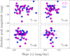 |
Fig. 5 Absolute (R/r-band) peak magnitude versus the absolute value of the slope parameters of the (R/r-band) light curves (γ). The SNe Ibn from the F25 and Lit samples are presented as magenta and blue circles, respectively. The top-left, top-right, and bottom-right panels show the light curve slopes γ−10 (−10 to tmax), γ+10 (tmax to day +10), γ+20 (+10 to +20 days), and γ+30 (+20 to +30 days), respectively. |
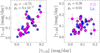 |
Fig. 6 Absolute values of the R/r-band slopes γ−10 (left panel) and γ+20 (right panel) versus γ+10. The numbers within each plot are the Spearman’s coefficients and p-values for γ−10 versus γ+10 (left) and for γ+20 versus γ+10 (right). The SNe Ibn from the F25 and Lit samples are presented as magenta and blue circles, respectively. |
4 Light curve modeling
To investigate the properties of the SN Ibn progenitor systems and surrounding CSM, we model the multiband light curves of SNe using MOSFiT8 (Guillochon et al. 2018). This work represents the largest consistently modeled sample of Type Ibn SNe in the literature. MOSFiT estimates the posterior distributions of the parameters for a specific model given the photometric observations and a set of user-defined prior distributions for such parameters.
For this purpose, we selected 24 SNe from the F25+Lit sample that have photometric data covering the B, V, g, c, r, o, R, I, and z bands, each with a cadence of ≲ 5 days and are well-sampled prior to maximum. The selected SNe Ibn are SN 2010al (Pastorello et al. 2015a), OGLE-2012-SN-006 (Pastorello et al. 2015e), SN 2014av (Pastorello et al. 2016), OGLE-2014-SN-131 (Karamehmetoglu et al. 2017), iPTF14aki and iPTF15ul (Hosseinzadeh et al. 2017), SN 2015U (Pastorello et al. 2015d; Shivvers et al. 2016), PS15dpn (Smartt et al. 2016), SN 2018jmt (Wang et al. 2024b), SN 2019uo (Gangopadhyay et al. 2020), SNe 2019deh and 2021jpk (Pellegrino et al. 2022b), SN 2019kbj (Ben-Ami et al. 2023), SN 2020bqj (Kool et al. 2021), SN 2020nxt (Wang et al. 2024a), SN 2022ablq (Pellegrino et al. 2024), SN 2023emq (Pursiainen et al. 2023), SNe 2020able, 2022ihx, 2022pda, 2023iuc, 2023qre, 2023rau, and 2023xgo (from F25). We refer to this sample as the MOSFiT sample (see Fig. 1).
We adopted the pure CSM-SN ejecta interaction model of MOSFiT (CSI) described in detail in Chatzopoulos et al. (2012, 2013); Villar et al. (2017). We chose the CSI model based on the moderate nickel masses found typically in SNe Ibn from light curve modeling (≲ 0.2 M⊙; Kool et al. 2021; Gangopadhyay et al. 2022; Ben-Ami et al. 2023; Farias et al. 2024) and the absence of a nickel radioactive tail (e.g., Gorbikov et al. 2014; Shivvers et al. 2016). The CSI model describes the total SN luminosity with a combination of CSM parameters and SN ejecta parameters. The CSM parameters are the optical CSM opacity (κ), CSM mass (MCSM), inner radius of the CSM (R0), CSM density (ρCSM), and the index of the density profile (s) of the CSM (ρCSM ∝ r−s). The SN ejecta parameters are the total mass of the SN ejecta (Mej), the inner (δ) and outer (n) indexes of the density profile of the ejecta (ρinner,ej ∝ r−δ and ρouter,ej ∝ r−n), and the ejecta velocity (vej). The parameter “n” describes the exponent of the outer velocity profile of the progenitor itsef, therefore it is a measure of the compactness of the progenitor envelope. Additional parameters of the CSI model are the hydrogen column density of the host galaxy (nH,host), the explosion time relative to the first detection (texp), the minimum temperature before the photosphere starts to recede (Tmin), the efficiency coefficient of converting kinetic energy to radiation (ϵ) and a white noise term (σ) to account for underestimation of the reported photometric uncertainties. We fix the inner slope of the SN ejecta (δ = 1) and the efficiency coefficient of kinetic energy to radiation (ϵ = 0.5). The former has a minimal effect on the light curve, while the latter has been to shown to vary between ~0.3–0.7 in Type IIn SNe (see Dessart et al. 2015; Ransome & Villar 2024). To test whether the contribution of the radioactive nickel decay to the light curves is small for SNe Ibn, we also model the multiband light curves of all 24 SNe using the 56Ni radioactive decay + CSM interaction (RD+CSI) from MOSFiT. This adds two more parameters with respect to the CSI model: the γ-ray opacity (Kγ) of the SN ejecta and the nickel fraction of the ejecta mass (fNi), following the prescription developed by Arnett & Fu (1989); Chatzopoulos et al. (2009). Each free parameter has the same prior distribution in each individual SN except for the lower boundary of the uniform distribution of the explosion time, which is set based on the observations of each object. The prior distributions of the parameters in the MOSFiT modeling are either uniform (𝒰) or log-uniform (log 𝒰), with the exception of the distribution of the ejecta velocity. For the latter, we assume a Gaussian (𝒢) distribution centered at 6000 km/s with a standard deviation of 2000 km/s and lower and upper limits of 3000 and 20 000 km/s, respectively. This is justified because velocity components larger than about 8000 km/s are rarely seen in the line profiles of SNe Ibn (e.g., Pastorello et al. 2016, see also Sect. 6).
4.1 Modeling results
For each SN in the MOSFiT sample, we sampled the posterior distributions of the parameters for both the CSI and RD+CSI models using the dynesty sampler implemented in MOSFiT. Tables D.4 and D.5 present the median values and the 50th-16th and 84th-50th percentiles of the marginalized distribution of each parameter (e.g., ρCSM), for each SN in the MOSFiT sample, for the CSI and RD+CSI models, respectively. Tables D.4 and D.5 show that the inferred values of the MOSFiT parameters for the CSI and RD+CSI encompass wide ranges; most notably, R0 and ρCSM. For 20 out of the 24 SNe in the MOSFiT sample, the CSM and ejecta masses inferred by the CSI and RD+CSI models are below 3 M⊙. For the CSI case, we find that n < 9 for 22 SNe in the MOSFiT sample. These values are smaller than those seen for the characteristic density profile of a red supergiant star (n = 12; Matzner & McKee 1999) and closer to characterizing a progenitor with a compact envelope (n ≲ 10), such as a luminous blue variable (LBV) or Wolf–Rayet (WR) star (Colgate & McKee 1969). For the RD+CSI, the values of n are larger than for the CSI case (n > 9), although they are still consistent within the typical uncertainties of the parameter in both models. Moreover, for the CSI model, s > 1 for 22 out of 24 SNe. These values imply that the CSM geometry is more wind-like (i.e, formed by steady mass loss based on s = 2), rather than an eruptive episode (shell-like, s = 0). However, the values of s for RD+CSI do not display any preference. For the nickel masses in the RD+CSI case, we obtain MNi ≲ 0.01 M⊙ for 20 out of 24 SNe in the MOSFiT sample. This is consistent with the lower limit of nickel masses obtained for SNe Ibc (0.03 − 0.012 M⊙; Meza & Anderson 2020; Afsariardchi et al. 2021; Rodríguez et al. 2023). Assuming that the energy of the SN explosion is proportional to ![Mathematical equation: $\[M_{\mathrm{ej}} v_{\mathrm{ej}}^{2}\]$](/articles/aa/full_html/2026/04/aa55954-25/aa55954-25-eq3.png) , the explosion energies of the SNe Ibn in the MOSFiT sample are below 1051 erg.
, the explosion energies of the SNe Ibn in the MOSFiT sample are below 1051 erg.
Figure 7 shows the median values of each parameter for each SN in the MOSFiT sample, including the PDFs in the diagonal. The PDFs are obtained using the (Gaussian) kernel density estimation (KDE) package from scipy.stats9. Evidently, the PDF of n for the CSI model is skewed towards the lower boundary of their prior distributions (n ~ 7). The explosion dates (relative to the peak magnitude) cluster close to ~ − 10 days. The clear outlier at texp = ![Mathematical equation: $\[-48.9_{-3.2}^{+2.2}\]$](/articles/aa/full_html/2026/04/aa55954-25/aa55954-25-eq4.png) days, OGLE-2014-SN-131, has the longest rise-time of all SNe Ibn (Karamehmetoglu et al. 2017). The most intriguing findings of the light curve modeling are the bimodal distributions for ρCSM and R0, and their potential correlation. The modeling results show that the densest CSM (i.e., ρCSM ≳ 10−14 g/cm3), is located closest to the progenitor star (i.e., R0 ≲ 2 × 1014 cm). For the SNe Ibn best described by these values, the median values of the ejecta parameters, Mej and vej, are also tightly constrained, with Mej ≲ 1 M⊙ and vej ≲ 5000 km/s. For SNe Ibn with less dense CSM (i.e., ρCSM < 10−14 g/cm3), we find that R0 > 2 × 1014 cm, n ≲ 10 and s ≳ 1. For the CSI case, we note that the three SNe Ibn in our MOSFiT sample (OGLE-2012-SN-006, SN 2021jpk and SN 2022pda) with the largest ejecta masses (> 10 M⊙) have low CSM densities. Irrespective of the model and density, the PDF of the CSM mass of the SNe of the MOSFiT sample peaks at ~0.1 M⊙, and of the ejecta masses at ~1.0 M⊙.
days, OGLE-2014-SN-131, has the longest rise-time of all SNe Ibn (Karamehmetoglu et al. 2017). The most intriguing findings of the light curve modeling are the bimodal distributions for ρCSM and R0, and their potential correlation. The modeling results show that the densest CSM (i.e., ρCSM ≳ 10−14 g/cm3), is located closest to the progenitor star (i.e., R0 ≲ 2 × 1014 cm). For the SNe Ibn best described by these values, the median values of the ejecta parameters, Mej and vej, are also tightly constrained, with Mej ≲ 1 M⊙ and vej ≲ 5000 km/s. For SNe Ibn with less dense CSM (i.e., ρCSM < 10−14 g/cm3), we find that R0 > 2 × 1014 cm, n ≲ 10 and s ≳ 1. For the CSI case, we note that the three SNe Ibn in our MOSFiT sample (OGLE-2012-SN-006, SN 2021jpk and SN 2022pda) with the largest ejecta masses (> 10 M⊙) have low CSM densities. Irrespective of the model and density, the PDF of the CSM mass of the SNe of the MOSFiT sample peaks at ~0.1 M⊙, and of the ejecta masses at ~1.0 M⊙.
As can be seen from Fig. 7, the PDFs of vej, Mej and texp for the RD+CSI model are similar to those of the CSI model, suggesting that these parameters are insensitive to the addition of the radioactive powering source. The largest differences between the shapes of the PDFs of the two models are noticeable for the index of the density profile of the CSM (s) and the outer SN ejecta (n). The bimodality in the PDFs of ρCSM and R0 for the CSI case is not as prominent in the RD+CSI scheme. Overall, the values of the host extinction (AV) for the CSI model is about a factor of 100 less than the one resulting from the RD+CSI model. The result of the CSI model suggests that there is negligible host galaxy extinction. Since about half of the SNe in the MOSFiT sample have accurate host galaxy extinction from previous studies, we expect that AV ≈ 0 for the MOSFiT sample.
Since 13 SNe out of the MOSFiT sample have been extensively studied elsewhere (see Table D.8 for references), we can broadly compare these results with our CSI and RD+CSI modeling results. Nickel masses have been estimated for SNe 2014av (Pastorello et al. 2016), 2015U (Shivvers et al. 2016), 2019uo, 2019deh, 2021jpk, iPTF15ul (Pellegrino et al. 2022b), PS15dpn (Wang & Li 2020), 2019kbj (Ben-Ami et al. 2023), 2020nxt (Wang et al. 2025), 2023emq (Pursiainen et al. 2023), 2023xgo (Gangopadhyay et al. 2025) and 2020bqj (Kool et al. 2021). These studies obtained nickel masses within 10−2−10−1 M⊙, about one dex higher than our results. Ejecta masses of SNe 2018jmt (Wang et al. 2024b), 2019uo, 2021jpk, iPTF15ul, 2019kbj (Ben-Ami et al. 2023), 2020nxt, 2023emq and 2023xgo have been estimated to be ≲ 2 M⊙. These values agree with our median values for the majority of the SNe in the MOSFiT sample, for any configuration. However, Kool et al. (2021), Karamehmetoglu et al. (2017) and Wang & Li (2020) reported ejecta masses > 10 M⊙ for SNe Ibn 2020bqj, OGLE-2014-SN-131 and PS15dpn, respectively. We only obtain such massive ejecta for SN 2020bqj from the RD+CSI model (~20 M⊙) and SNe 2021jpk, 2022pda and OGLE-2012-SN-006 for the CSI model (~10 M⊙). Discrepancies in the nickel and the ejecta masses are related to the underlying models used to estimate these parameters. For example, Pastorello et al. (2015e) did not use a CSI model to estimate the ejecta and nickel masses inferred for OGLE-2012-SN-006. Instead, they used a pure radioactive decay model, obtaining an ejecta mass of ~2 M⊙, with a nickel mass of ~1 M⊙. This nickel mass is larger than the maximum value observed for SNe Ibc (~0.7 M⊙; Rodríguez et al. 2023). The CSM masses estimated in previous studies (e.g., Pursiainen et al. (2023); Pellegrino et al. (2022b) are typically of the order of ~0.1 M⊙, consistent with our findings.
4.2 Modeling caveats
MOSFiT and similar codes (e.g., Chatzopoulos et al. 2013; Sarin et al. 2024) aim at modeling the light curves of different types of SNe. Hence, these models explore a large parameter space and the results are affected by the prior distributions of the parameters. Here, we test whether a change of the prior distributions of vej, a Gaussian distribution centered at μ = 8000 km/s with σ = 2000 km/s, and of ρCSM, a log-Uniform distribution between 10−18 and 10−8 g/cm3, 𝒰(10−18, 10−8), affect the results obtained for the CSI and RD+CSI modeling. We refer to the original set and the set of test prior distributions as PRIOR A and PRIOR B, respectively.
Independent of the choice of prior (A or B), the main relations between different parameters shown in Fig. 7 are preserved. However, for some individual SNe, there are large discrepancies between the median values of several parameters, such as ρCSM and R0. These discrepancies involve changes from either low to high values or vice versa. These changes could imply that the posterior distributions of the MOSFiT parameters are multi-modal and, thus, our sampling routine might not be adequate for capturing these complex distributions.
Figure 8 shows the relation between between R0 and ρCSM for the CSI and RD+CSI model, given the PRIOR A or PRIOR B. The width of the prior distribution of ρCSM has a direct impact on the median value of the posterior distribution of ρCSM, with a preference for large densities (~10−8 g/cm3) for PRIOR B. The Spearman’s rank coefficients for the CSI model are both ρs ~ −0.9, with a p-value pval < 10−6, suggesting a strong anticorrelation. This anticorrelation is not as prominent for the RD+CSI model, perhaps due to the larger number of free parameters involved in the latter. However, we emphasize that this anticorrelation might not be real. Instead, the evident relation between R0 and ρCSM might be a degeneracy of the model (see Appendix B).
In summary, irrespective of the choice of the prior distribution and the model, the correlation between ρCSM and R0 remains, suggesting that there is a degeneracy inherent to the modeling of the circumstellar interaction. Nevertheless, both both CSI and RD+CSI models share some results such as CSM masses below 1 M⊙, ejecta masses below 10 M⊙, ejecta velocities below 10 000 km/s, and s ≳ 0.5.
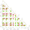 |
Fig. 7 Inferred values of seven MOSFiT parameters for all 24 SNe in the MOSFiT sample. The parameters shown here are log Mej, vej, log MCSM, log ρCSM, with ρCSM in units of 10−12 g/cm3, log R0, with R0 in units of 1014 cm, s, n, and texp for the CSI (circle) and RD+CSI (square) models. The blue circle in each plot highlights the Type Ibn OGLE-2014-SN-131. For the CSI sample, the lime and crimson circles correspond to the SNe with ρCSM above or below 10−14 g/cm3, respectively. Probability density functions (PDFs) produced with a Gaussian kernel density estimator are shown along the diagonal. Black and yellow curves correspond to the PDF of a specific parameter for the CSI and RD+CSI models, respectively. The subplot with red axes highlights the correlation between ρCSM and R0, which is further explored in Fig. 8. |
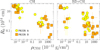 |
Fig. 8 Left: median values of the posterior distributions of R0 versus ρCSM for each SN in the MOSFiT sample under the CSI model, using prior distributions A (yellow circles) and B (orange squares). Right: same as the left panel, but for the RD+CSI case. |
5 X-ray analysis
Prior to this study, only SNe Ibn 2006jc (Immler et al. 2008) and 2022ablq (Pellegrino et al. 2024) had reported X-ray detections. In this work, we analyze the XRT observations of 15 SNe (see the X-RAY sample in Fig. 1 and Sect. 2.1.2) of the F25 sample (Table D.6). Apart from SN 2022ablq, SN 2022qhy, SN 2020nxt, and SN 2023emq, we did not detect X-ray emission at the positions of the SNe. Furthermore, the detected X-ray emission of SNe 2020nxt and 2022qhy is likely to come from the host galaxy. The X-ray emission associated with SN 2023emq on day +11 is only a 2σ detection. Since we only retrieved upper limits from XRT observations of SN 2023emq after this epoch, the X-ray emission at day +11 might be a spurious detection.
The powering source of the soft (0.1–10 keV) and hard (>10 keV) X-ray light curve of Type Ibn SNe is primarily free-free emission from electrons at the forward (i.e., circumstellar) shock region (Inoue & Maeda 2024). There are only small contributions (Margalit et al. 2022) from inverse Compton scattering of photons by the shocked electrons at the interaction region of the forward shock (Chevalier & Fransson 2017) and possible a co-existing reverse shock (e.g., Fransson et al. 2014). The X-ray light curves (LX) of SNe 2006jc and 2022ablq share similar shapes, which can be parameterized by two power laws with respect to the X-ray peak luminosity (Pellegrino et al. 2024). The pre-maximum X-ray light curves of SNe 2006jc and 2022ablq follow a power law defined as LX ∝ t. The post-maximum X-ray light curve of SN 2006jc follows a power law LX ∝ t−3.1, while LX ∝ t−1.8 for SN 2022ablq.
The evolution of the post-maximum X-ray light curves of both SNe imply that the CSM is not necessarily a result of a steady mass-loss process (index of the density profile, s = 2, e.g., Dwarkadas & Gruszko 2012), with a typical decline LX ∝ t−1 to t−2 (Fransson et al. 1996, and see e.g., Figure 13 of Panjkov et al. 2024 and references therewithin). Nevertheless, for simplicity and given the single detections and upper limits of several SNe Ibn in the X-RAY sample, we set s = 2 for our X-ray analysis. Under the assumption of a negligible contribution of the reverse shock to the total X-ray luminosity, Dwarkadas et al. (2016) approximated the luminosity at 1 keV (LCS,1keV) as
![Mathematical equation: $\[\begin{aligned}L_{\mathrm{CS}, 1 ~\mathrm{keV}}= & 1.4 \times 10^{38} \xi T_8^{-0.236} \frac{e^{-0.116 / T_8}}{(3-s)}\left[\frac{\dot{M}_{-5}}{v_w}\right]^2 \\& \times v_{\mathrm{ej}, 4}^{3-2 s}\left[\frac{t_X}{11.57}\right]^{3-2 s} \quad \mathrm{erg} / \mathrm{s} / \mathrm{keV},\end{aligned}\]$](/articles/aa/full_html/2026/04/aa55954-25/aa55954-25-eq5.png) (1)
(1)
where T8 is the shock temperature in units of 108 K, ![Mathematical equation: $\[\dot{M}_{-5}\]$](/articles/aa/full_html/2026/04/aa55954-25/aa55954-25-eq8.png) is the mass-loss rate scaled to 10−5 M⊙/yr, vw is the wind velocity in terms of 10 km/s, vej, 4 is the maximum ejecta velocity in units of 104 km/s, ξ ~ 0.85, and tX is the duration of the X-ray event. We can determine
is the mass-loss rate scaled to 10−5 M⊙/yr, vw is the wind velocity in terms of 10 km/s, vej, 4 is the maximum ejecta velocity in units of 104 km/s, ξ ~ 0.85, and tX is the duration of the X-ray event. We can determine ![Mathematical equation: $\[\dot{M}\]$](/articles/aa/full_html/2026/04/aa55954-25/aa55954-25-eq9.png) from Eq. (1) assuming T, vw, vej, LCS, 1 keV and tX. From the mean values of the PDFs of the narrow and broad velocity components of He I λ5876 Å in Sect. 6, we set vw ≈ 1000 km/s and vej ≈ 5000 km/s. Furthermore, we adopted a conservative value of the shock temperature (T8 ~ 1; Nymark et al. 2009). The quantities LCS, 1 keV, and tX are estimated directly from the Swift XRT observations (Table D.6). The duration of the X-ray event is defined as the average date of the combined XRT observations relative to the discovery date of the supernova. The total X-ray luminosity at 1 keV (LCS, 1 keV) was estimated as the XRT luminosity scaled by the passband width of XRT, from 10 keV to 0.3 keV. The left panel of Fig. 9 shows the mass-loss rates inferred for each SN based on the X-ray data. Most of these measurements represent upper limits. By construction, higher wind velocities results in correspondingly higher mass-loss rate estimates. For the vast major of SN in our sample, we observe that the upper limits of the mass-loss rates from the X-ray analysis are largely consistent with the results obtained using MOSFiT (Tables D.4 and D.5). We find that the mass-loss rates of SN 2022ablq is about 1 M⊙/yr from our X-ray analysis, which is about twice the value reported in Pellegrino et al. (2024, ≲ 0.5 M⊙/yr).
from Eq. (1) assuming T, vw, vej, LCS, 1 keV and tX. From the mean values of the PDFs of the narrow and broad velocity components of He I λ5876 Å in Sect. 6, we set vw ≈ 1000 km/s and vej ≈ 5000 km/s. Furthermore, we adopted a conservative value of the shock temperature (T8 ~ 1; Nymark et al. 2009). The quantities LCS, 1 keV, and tX are estimated directly from the Swift XRT observations (Table D.6). The duration of the X-ray event is defined as the average date of the combined XRT observations relative to the discovery date of the supernova. The total X-ray luminosity at 1 keV (LCS, 1 keV) was estimated as the XRT luminosity scaled by the passband width of XRT, from 10 keV to 0.3 keV. The left panel of Fig. 9 shows the mass-loss rates inferred for each SN based on the X-ray data. Most of these measurements represent upper limits. By construction, higher wind velocities results in correspondingly higher mass-loss rate estimates. For the vast major of SN in our sample, we observe that the upper limits of the mass-loss rates from the X-ray analysis are largely consistent with the results obtained using MOSFiT (Tables D.4 and D.5). We find that the mass-loss rates of SN 2022ablq is about 1 M⊙/yr from our X-ray analysis, which is about twice the value reported in Pellegrino et al. (2024, ≲ 0.5 M⊙/yr).
Margalit et al. (2022) studied the X-ray luminosity coming from the shock due to free-free emission and Compton ionization, for different shock regimes (radiative or adiabatic). They constructed the parameter space ![Mathematical equation: $\[\tilde{v} L_{X} / v_{X}\]$](/articles/aa/full_html/2026/04/aa55954-25/aa55954-25-eq10.png) versus
versus ![Mathematical equation: $\[\tilde{v} t_{X}\]$](/articles/aa/full_html/2026/04/aa55954-25/aa55954-25-eq11.png) , where
, where ![Mathematical equation: $\[\tilde{v}=v_{\mathrm{sh}} / v_{\mathrm{rad}}\]$](/articles/aa/full_html/2026/04/aa55954-25/aa55954-25-eq12.png) is the ratio between the shock velocity (vsh) and the limiting velocity (vrad), and determines if a shock is either adiabatic or radiative. Using these variables, they obtain analytical expressions of the mass and radius of the CSM,
is the ratio between the shock velocity (vsh) and the limiting velocity (vrad), and determines if a shock is either adiabatic or radiative. Using these variables, they obtain analytical expressions of the mass and radius of the CSM,
![Mathematical equation: $\[M_{\mathrm{CSM}} \approx 0.11\left(\frac{\tilde{v} L_X / \nu_{\mathrm{keV}}}{10^{41} \mathrm{erg} / \mathrm{s}}\right)\left(\frac{\tilde{v} t_X}{100 \text { days }}\right) \mathrm{M}_{\odot},\]$](/articles/aa/full_html/2026/04/aa55954-25/aa55954-25-eq13.png) (2)
(2)
![Mathematical equation: $\[R_{\mathrm{CSM}} \approx 4.5 \times 10^{15}\left(\frac{\tilde{v} L_X / \nu_{\mathrm{keV}}}{10^{41} \mathrm{erg} / \mathrm{s}}\right)^{1 / 4}\left(\frac{\tilde{v} t_X}{100 \text { days }}\right)^{3 / 4} \mathrm{~cm}.\]$](/articles/aa/full_html/2026/04/aa55954-25/aa55954-25-eq14.png) (3)
(3)
Given the lack of a rich spectroscopic follow-up of several SNe in the X-RAY sample to trace the velocity of the shock and evaluate ![Mathematical equation: $\[\tilde{v}\]$](/articles/aa/full_html/2026/04/aa55954-25/aa55954-25-eq15.png) as done by Pellegrino et al. (2022b), we assumed
as done by Pellegrino et al. (2022b), we assumed ![Mathematical equation: $\[\tilde{v}=1\]$](/articles/aa/full_html/2026/04/aa55954-25/aa55954-25-eq16.png) . Similarly to Margalit et al. (2022), we assumed a characteristic frequency vX = 1 keV. Using Eqs. (2) and (3), we constrained the values of MCSM and RCSM for the SNe in the X-RAY sample, independently from the light curve analysis in Table D.4. The right panel of Fig. 9 shows that the CSM in SNe Ibn, including SN 2006jc (Immler et al. 2008), is much less massive (~0.1 M⊙) and more compact (RCSM < 1016 cm) than the most extreme Type IIn SNe 2010jl (Chandra et al. 2015) and 2006jd (Chandra et al. 2012).
. Similarly to Margalit et al. (2022), we assumed a characteristic frequency vX = 1 keV. Using Eqs. (2) and (3), we constrained the values of MCSM and RCSM for the SNe in the X-RAY sample, independently from the light curve analysis in Table D.4. The right panel of Fig. 9 shows that the CSM in SNe Ibn, including SN 2006jc (Immler et al. 2008), is much less massive (~0.1 M⊙) and more compact (RCSM < 1016 cm) than the most extreme Type IIn SNe 2010jl (Chandra et al. 2015) and 2006jd (Chandra et al. 2012).
 |
Fig. 9 Left: mass-loss rates versus the duration of the X-ray event of 15 Ibn SNe of the F25 sample observed with Swift XRT. The mass-loss rates were estimated using Eq. (1). Right: parameter space of Margalit et al. (2022), |
![Mathematical equation: $\[\tilde{v} L_{X} / v_{X}\]$](/articles/aa/full_html/2026/04/aa55954-25/aa55954-25-eq6.png)
![Mathematical equation: $\[\tilde{v} t_{X}\]$](/articles/aa/full_html/2026/04/aa55954-25/aa55954-25-eq7.png)
6 Analysis of helium lines
For SNe in the F25 sample as described in Sect. 2.2, we model the prominent He I λ5876 Å emission line to characterize the progenitor wind and ejecta velocities over time. All SNe of the F25 sample have at least one spectrum. The SN with the largest (unpublished) spectral series is SN 2020able, with spectra taken from −14 days to +20 days. The He I λ5876 emission line is visible in all spectra.
We designed a python program using the MCMC sampler emcee to obtain the posterior distributions of the set of parameters of the different components of the spectral lines. For this purpose, we subtracted the local continuum from the He I λ5876 Å by fitting a linear function to the background regions of the line. The two background regions are defined centered on ±200 Å of the λ5876 Å He I line complex, with a width of ~50 Å. We added an extra scatter parameter to the fitting to account for the white noise of the spectrum. The purpose of including this term is to estimate the noise in spectra published without any reported uncertainties, mainly from WISeREP. Thereafter, we fit the continuum-subtracted He I lines using a linear combination of Gaussian profiles. One Gaussian profile is fit to each distinct component of the He I line complex. The He I line complex is composed of a mixture of narrow and broad components. Some of the individual components also exhibit entire P-Cygni profiles, consisting of both emission and absorption components. Thus, the number of profiles to be fit for the He I line complex depends on the number of components, which we determined by visual inspection of each spectrum. We categorize any component of the He I λ5876 Å line complex with estimated velocity as the full width at half maximum (FWHM) lower than 3000 km/s as “narrow”. Similarly, a “broad” component refers to any emission component of the He I λ5876 Å line with a FWHM larger than 3000 km/s. Typically, the narrow emission component represents the velocity of the CSM, vCSM (see Sect. 1). In the case of a P-Cygni narrow profile, we determined the velocity from either the minimum of the narrow absorption component or the FWHM of the narrow emission component. We assumed the velocity of the broad component corresponds to the lower limit of the ejecta velocity. To fit the continuum and the Gaussian profiles of the He I λ5876 Å lines, we used 100 walkers for 10 000 steps with a MCMC fitter to sample the parameter space and obtain the posterior distributions of each parameter.
For each SN Ibn in the F25 sample with an associated spectral time series, we chose the highest velocity of all He I λ5876 Å broad components as the lower limit of the ejecta velocity for that SN. Similarly, we chose the lowest velocity of the He I λ5876 Å narrow components as the CSM velocity of that SN. However, we emphasize that this velocity is not the true velocity of the CSM. Instead, it is the lowest velocity (an upper limit) measurable from the available spectra without accounting for the spectral resolution of the instruments. For 21 out of 37 SNe in the Lit sample, we retrieved the spectra from WISeREP or private communication (e.g., SNe 2019wep, 2022ablq, and 2023emq) and analyzed the He I λ5876 Å emission lines following the same procedure as for the SNe in F25 (outlined above). For 14 SNe of the Lit sample (see Table D.2), not all the spectroscopic data from their analysis were published (e.g., P16, Smartt et al. 2016). In these cases, we take the velocity estimations of either the narrow or broad components that were reported. For the specific case of the P16 sample, we retrieved the minimum velocity of the narrow component as the CSM velocity and the maximum velocity of the broad component as the potential ejecta velocity of a SN (Table 7 in P16). For two SNe in the Lit sample (PTF11rfh and SN 2019qav), we could not obtain any estimates of the narrow or broad velocity components of the He I λ5876. In total, we collected te velocity estimates for 59 SNe for the F25 (24) + Ibn (35) samples. All 59 velocity estimates are listed in Table D.7.
Figure 10 shows the distribution and PDFs of the final CSM and ejecta velocities derived from the narrow and broad components of the complex He I λ5876 emission line profile for the 59 SNe Ibn. The PDFs were obtained using the method described in Sect. 4. Furthermore, we drew 106 samples from their PDFs to estimate the mean and standard deviations of the PDFs. The PDF of the narrow components peaks at a velocity of 1144 ± 487 km/s and the PDF of the broad components peaks at a velocity of 4847 ± 2038 km/s. The latter is consistent with previous works (e.g., P16, H17) and supports our assumption of the mean value of the prior distribution of the ejecta velocity for the MOSFiT light curve modeling (Sect. 4).
By integrating the PDF of the narrow velocity over the velocity range, we note that over 90% of our estimates are at v ≲ 2300 km/s. Therefore, we adopt v = 2300 km/s as a tentative threshold to classify Type Ibn SNe. However, this threshold is purely observational and dependent on the time at which the spectra were obtained, the resolution or S/N of the available spectra and how rich/poor the spectroscopic follow up was for a particular SN. Nevertheless, it is evident that unless the observation was performed with a low-resolution instrument (R ≲ 120 at He I λ5876 Å), or at late phases in the evolution of the SN, the threshold represents a practical benchmark for observers to characterize the Ibn class.
To visualize the variety of possible origins of the different components comprising the spectral lines, Fig. C.1 shows a compilation of the continuum-subtracted He I λ5876 Å line profiles of different SNe Ibn and at different epochs between one to three weeks after maximum light. About 50% of the SNe in the F25 sample exhibit narrow P-Cygni profiles of He I λ5876 Å throughout their evolution. For the remaining SNe Ibn at these epochs, the He I λ5876 Å is a pure emission line. Highlighted in Fig. C.1 is also the presence of Hα next to He I λ6678 Å which becomes stronger at later epochs in some SN Ibn spectra. This is not uncommon for SNe Ibn (see e.g., Pastorello et al. 2008a) since the He-rich CSM might be mixed with H-rich material which was not completely expelled from the progenitor star/system before the SN explosion (Farias et al. 2024). In higher resolution spectra of some SNe Ibn (e.g., SNe 2021iyt, 2022gzg, 2022ihx, 2023iuc, and 2023qre), the [N II] λλ6583, 6548 Å emission lines are identified next to Hα, suggesting a host galaxy origin for the hydrogen lines for some fraction of these objects.
At several days prior to peak (about −7 days), the emission lines are likely "flash-ionization features” (Khazov et al. 2016), such as those observed for SNe Ibn 2010al, 2015U, 2019cj (Wang et al. 2024b), 2019uo, 2019wep (Gangopadhyay et al. 2022), and 2023emq. Appendix Fig. C.2 shows the early spectra of all Ibn-like SNe known to date which have flash-ionization features. In the F25 sample, we can ascribe a flash-ionization origin of the blended complex of He II λ4686, N III λλ4634, 4641 and C III λλ4648, 4650 emission lines for nine SNe (20191sm, 2020able, 2021iyt, 2022eux, 2022ihx, 2023iuc, 2023qre, 2023rau, and 2023xgo), typically observed in early spectra of Type II SN (Jacobson-Galán et al. 2024b). Though blended, the spectral feature at ~4600Å shows wide wings, characteristic of the broadening of narrow lines due to the photons scattering off of the electrons in the ionized CSM. Furthermore, for eight SNe Ibn in F25 we identify the C III emission line at ≈ 5696 Å (SNe 20191sm, 2020able, 2021iyt, 2022ihx, 2023iuc, 2023qre, 2023rau, and 2023xgo) The presence of this line indicates a high ionization of the CSM and has so far only been observed in one SN Ibn, SN 2023emq (Pursiainen et al. 2023), although it is more common in spectra of Type II SNe, such as SN 1998S (Fassia et al. 2001).
We note that SNe that have identifiable He lines, relegating them to the class of Type Ib SNe, might not exhibit a narrow component at the time of classification. The reason behind this might be physical in origin (e.g., the ejecta have already swept up the entire CSM and, thus, no signatures remain in the spectra). This could be the case at either late epochs or early on, when only a marginal amount of CSM close to the progenitor is present. Alternatively, CSM velocities much less than about 1000 km/s can be missed in low(er) resolution spectra and with poor S/N. Some SNe Ibn have also been found with no broad He velocity components in their spectra. One such example is SN 2011hw, which does not exhibit any velocity component greater than 2350 km/s since its discovery up to +60 days past maximum light (Pastorello et al. 2016). On the other hand, it shows resolved narrow components of He I λ5876 Å (vnarrow ≈ 200 km/s), likely originating from the unshocked CSM. A SN can have either an unclear or missing broad velocity component of an emission line if the SN ejecta has been slowed to velocities hovering around ~2300 km/s through the interaction with a dense CSM. A broad velocity component could also be hidden by the photosphere created ahead of the ejecta in the CSM. Independently of the origin or mechanism leading to an absent broad velocity component, it would only affect the classification of a SN Ibn if, additionally, no narrow component is present or can be identified.
With our derived estimates of the CSM velocity (vCSM), we can estimate the average mass-loss rate for each SN in the MOSFiT sample, following Eq. (4) from Ransome & Villar (2024) and expressed as
![Mathematical equation: $\[\langle\dot{M}\rangle \approx \frac{4 \pi \rho_{\mathrm{CSM}} R_0 v_{\mathrm{CSM}}}{3-s} R_{\mathrm{CSM}, \text {outer}}^{2-s},\]$](/articles/aa/full_html/2026/04/aa55954-25/aa55954-25-eq17.png) (4)
(4)
with
![Mathematical equation: $\[R_{\mathrm{CSM}, \text {outer}}=\left(\frac{3 M_{\mathrm{CSM}}}{4 \pi \rho_{\mathrm{CSM}} R_0^s}+R_0^{3-s}\right)^{\frac{1}{3-s}},\]$](/articles/aa/full_html/2026/04/aa55954-25/aa55954-25-eq18.png) (5)
(5)
using samples from the full joint posterior distribution of ρCSM, R0, MCSM and s for each SN, thereby preserving correlations among parameters (Sect. 4, Tables D.4 and D.5).
Using Eq. (4), the mass-loss rates of the 17 SNe of MOSFiT sample for the CSI case are ![Mathematical equation: $\[\dot{M}\]$](/articles/aa/full_html/2026/04/aa55954-25/aa55954-25-eq19.png) ≲ 0.1 M⊙/yr (see Table D.4). This value (≳ 10−3 M⊙/yr) is consistent with the typical mass-loss rates found in the late stages of the mass-transfer episodes for binary systems of helium star + compact object (e.g., Wu & Fuller 2022). For the RD+CSI case, the mass-loss rate values are larger than for the CSI case, with 11 SNe having mass-loss rates over 1 M⊙/yr. The values of the outer radius of the CSM (Router,CSM) for 18 SNe in the MOSFiT sample (RD+CSI) are ≲ 1016 cm, consistent with the constraints found from our X-ray analysis. Larger values of Router,CSM are found for the CSI case. For the latter, 50% of the SNe in the MOSFiT sample have Router,CSM >1016 cm.
≲ 0.1 M⊙/yr (see Table D.4). This value (≳ 10−3 M⊙/yr) is consistent with the typical mass-loss rates found in the late stages of the mass-transfer episodes for binary systems of helium star + compact object (e.g., Wu & Fuller 2022). For the RD+CSI case, the mass-loss rate values are larger than for the CSI case, with 11 SNe having mass-loss rates over 1 M⊙/yr. The values of the outer radius of the CSM (Router,CSM) for 18 SNe in the MOSFiT sample (RD+CSI) are ≲ 1016 cm, consistent with the constraints found from our X-ray analysis. Larger values of Router,CSM are found for the CSI case. For the latter, 50% of the SNe in the MOSFiT sample have Router,CSM >1016 cm.
Mass-loss rates have been estimated for several SNe Ibn from light curve modeling (Wang & Li 2020; Gangopadhyay et al. 2022; Shivvers et al. 2016; Pellegrino et al. 2022b) and X-ray analysis (Pellegrino et al. 2024). Apart from PS15dpn (~8 M⊙/yr), the mass-loss rates estimated in the previous studies are ~1 M⊙/yr, similar to the values we estimated for the CSI and RD+CSI models (Tables D.4 and D.5). However, for SN 2022ablq, we obtained a mass-loss rate of ![Mathematical equation: $\[8.6_{-1.5}^{+2.0}\]$](/articles/aa/full_html/2026/04/aa55954-25/aa55954-25-eq20.png) M⊙/yr from MOSFiT modeling (from either CSI or RD+CSI models), as opposed to ≈ 1 M⊙/yr from our X-ray analysis. The discrepancy between the mass-loss rate values of SN 2022ablq are due to differences of the assumed wind velocity and several assumptions we had to make to properly evaluate Eq. (1). For instance, when using vw = 1000 km/s in Eq. (4), the MOSFiT mass-loss rate for SN 2022ablq ends up decreasing to ≈ 3 M⊙/yr.
M⊙/yr from MOSFiT modeling (from either CSI or RD+CSI models), as opposed to ≈ 1 M⊙/yr from our X-ray analysis. The discrepancy between the mass-loss rate values of SN 2022ablq are due to differences of the assumed wind velocity and several assumptions we had to make to properly evaluate Eq. (1). For instance, when using vw = 1000 km/s in Eq. (4), the MOSFiT mass-loss rate for SN 2022ablq ends up decreasing to ≈ 3 M⊙/yr.
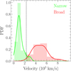 |
Fig. 10 PDF of the narrow (lime) and broad (red) velocity components of He I λ5876 lines of 59 SNe Ibn derived using KDE (solid lines). Lime and red histograms correspond to the empirical velocities used to estimate the corresponding PDFs, assuming these components are resolved. The dashed black line marks v = 2300 km/s. |
7 Discussion
We present a comprehensive analysis of a rich set of photometric and spectroscopic data for 24 SNe Ibn (F25 sample) observed by the Young Supernova Experiment between 2019 and 2023. We augmented the F25 sample with a photometric and spectroscopic dataset of 37 SNe Ibn (Lit sample) from the literature (see Fig. 1, Sect. 3, Table D.8) Our detailed light curve analysis shows that there is a high degree of heterogeneity in brightness, color, and light-curve shape and evolution, which has not been apparent in previous studies (e.g., P16, H17) of small samples of SNe Ibn. In particular, the normalized R/r-band light curves of the 61 SNe Ibn in our F25+Lit sample (Fig. 3, bottom panel) show a large spread (> 1.5 mag) with respect to known SNe Ibn templates at late times (~ + 50 days) (H17; Khakpash et al. 2024). Furthermore, there is no noticeable common evolutionary path for either B − V or g − r color curves for any SN in our F25+Lit sample (Fig. 2). Based on our measurements, we do not find any correlation between the peak magnitudes and decay slope for our SNe Ibn (Sect. 3). However, there is a clear correlation between the rise and decay slopes of our SNe Ibn, with faster evolving SNe having steeper slopes. The study of the origin of the rapidly evolving nature of the LCs of SNe Ibn is beyond the scope of this paper. However, its origin might be related, for example, to short photon diffusion times (e.g., Chevalier & Irwin 2011), short-lived powering mechanisms such as SN ejecta-CSM interaction (e.g., Wang & Li 2020), or asymmetries in the SN ejecta/CSM (Suzuki et al. 2019), among others.
Typically, the main mechanism that powers the light curves of stripped-envelope SNe is the release of the shock energy deposited in the SN ejecta (Villar et al. 2017). Other potential heating sources include the chain of radioactive decay of 56Ni and interaction between the SN ejecta and the CSM. In the absence of the latter two, the light curve of a stripped-envelope SN is mostly determined by the kinetic energy of the SN explosion (or the ejecta velocity) and the ejecta mass. This means that for a fixed kinetic energy, the higher the ejecta mass, the longer the duration of the light curve. For a fixed ejecta mass, the more energetic the SN explosion, the higher the SN luminosity. Since slowly evolving SNe Ibn are rare (Fig. 3), the ejecta masses of most of the SNe Ibn are not expected to be high (~10 M⊙). Furthermore, the absence of a radioactive tail in the light curves of SNe Ibn suggests that the nickel mass must also be low (≲ 0.1 M⊙; Moriya & Maeda 2016). Thus, for the majority of our sample, a direct, rapid interaction between the SN ejecta and a nearby, compact CSM is the most plausible scenario. However, as suggested by the diversity seen in the photometry and spectroscopy, the mechanism powering the slow light curve evolution of some SNe Ibn in our sample may be more complex. It is possible that the SN ejecta-CSM interaction might cause photometric evolution that mimics the effect of large ejecta masses.
To elucidate possible mechanisms driving the photometric heterogeneity of SNe Ibn found in this study, we modeled the well-sampled light curves of 24 SNe Ibn (MOSFiT sample, see Sect. 4), using the csm (CSI) and csmni (RD+CSI) models implemented in MOSFiT. We find that median rise times (~10 days), CSM (≈ 0.1 M⊙) and ejecta masses (~1.0 M⊙), and the index of the density profile of the SN ejecta (n ≲ 10) inferred from most of the SNe in the MOSFiT sample are consistent between both models (Table D.4, Fig. 7). Rise times of ~10 days were also estimated from the photometric analysis in H17. A rapid photometric evolution suggests that radioactive 56Ni decay does not play a major role as an additional powering source, especially at late times. Our RD+CSI modeling leads us to conclude that the light curves in our MOSFiT sample are powered by the radioactive decay of small amounts (<0.01 M⊙) of 56Ni. These nickel masses are lower than the average nickel masses obtained for SNe Ibc (0.09±0.005 M⊙; Rodríguez et al. 2023) and consistent with the little-to-no nickel masses derived from the bolometric light curves of several SNe Ibn (Maeda & Moriya 2022). This again supports the interpretation of the power source as comprised primarily of SN ejecta interacting with a nearby CSM. The low CSM and ejecta masses inferred from light curve modeling suggest that the compact progenitor of most SNe in our sample must not necessarily be a massive Wolf–Rayet star at the moment of explosion (~ 10 M⊙; Massey 1981), as hypothesized in early studies (e.g., Foley et al. 2007). The findings of SNe Ibn in low star-forming regions (Sanders et al. 2013; Warwick et al. 2024) also support that their progenitors may not be massive stars. Recently, Ercolino et al. (2024) found that a binary system composed of a low-mass (~3 M⊙) helium-rich star and a main sequence star can produce an asymmetric CSM with MCSM ≲ 0.8 M⊙. Such scenario is suggested for the progenitor system of SN 2020nxt (Wang et al. 2024a). In Ercolino et al. (2024), the CSM formation happens through several mass transfer episodes via Roche-lobe overflow or "effective ROLF” (1 ± e)xRLOF (see section 2.3 in Hamers & Dosopoulou 2019). The CSM can then be understood as a circumbinary disk (Lu et al. 2023). The helium star, if it explodes as a CCSN, would eject ≲ 2 M⊙. Similar results were found for a low-mass helium star with a neutron star as a companion (Wu & Fuller 2022). Such binary scenarios were also proposed to explain the precursor emission observed in SNe 2006jc (Foley et al. 2007), 2019uo (Strotjohann et al. 2021), and 2023fyq (Dong et al. 2024).
Although consistent between different models and prior distributions of the parameters, our MOSFiT modeling results are obtained assuming a spherically symmetric CSM geometry. An asymmetric CSM, such as that produced by the binary progenitor system proposed for SNe Ibn (Ercolino et al. 2024), which is typically observed from specific viewing angles, could be responsible for the appearance (or absence) of P-Cygni profiles in SNe Ibn. This hypothesis was proposed by H17 to account for the roughly equal ratio between SNe Ibn with P-Cygni versus emission lines. Alternatively, optical depth and/or density effects have been suggested for the origin of P-Cygni versus emission lines (Karamehmetoglu et al. 2021). About 50% of the SNe in the F25 sample show P-Cygni profiles in the He I λ5876 Å, a ratio similar to that found by H 17. Therefore, the assumption of a spherical symmetric CSM would break down. This is a limitation of the available tools to model SNe observations, and more detailed models accounting for an asymmetric CSM geometry, and detailed spectropolarimetric observations of SNe Ibn are needed to more completely understand the geometry of the CSM and the nature of the progenitor systems.
Our spectroscopic analysis of 59 SNe Ibn shows that throughout the evolution, the median velocity of the broad component of the He I λ5876 Å line (vbroad) is ≈ 5000 km/s. This velocity might be considered a lower limit of the ejecta velocity (vej) in SNe Ibn. Similarly, for the CSM velocity, we adopt the upper limit of the narrow velocity component as measured in our spectroscopic analysis. In practice, this assumption is only valid for resolved spectral lines. Assuming that the MOSFiT CSI modeled ejecta velocity is accurate, then Fig. 11 (bottom-right panel) shows that vbroad does not follow a 1:1 relation with MOSFiT vej. In principle, vej < vbroad is plausible if the SN ejecta has decelerated during the interaction with the CSM. In this case, prominent emission lines will not have a broad velocity component. However, several SNe Ibn show vbroad > vej, with some extreme cases such as SNe 2019kbj and 2022ihx (> 8000 km/s). In the latter case, an asymmetric CSM configuration may be hiding a portion of the SN ejecta that is interacting with the CSM, making a broad velocity component visible. Furthermore, despite the large uncertainties, we do not observe any correlation between MCSM and vCSM (Fig. 11, top-left panel). Similarly, there is no apparent correlation between either the CSM velocity with the CSM density or the broad velocity and the sum of the SN ejecta and CSM masses (Fig. 11, top-right and bottom-left panels, respectively). The lack of any apparent correlation between the spectroscopic and the (modeled) photometric features shows that it is not straightforward to reconcile spectroscopic and photometric-derived information of SNe Ibn. These results reinforce that the CSM configuration is more complex than currently captured by light curve models such as MOSFiT. Moreover, Wang et al. (2024b) found that the light curves of the SNe Ibn 2018jmt and 2019cj may be well-fitted by more than one CSM region, also indicating an asymmetric CSM. Further development of such models accounting for either multiple CSM shells or asymmetric geometries is critical to understanding the explosion physics of SNe Ibn. Moreover, consideration in future tools may also be given to additional information derived from the spectroscopic evolution of SNe Ibn, such as the different line velocities of characteristic elements.
8 Conclusions
In this work, we analyzed the photometric and spectroscopic data of 24 SNe Ibn observed through the Young Supernova Experiment from 2020 to 2023 (see Tables D.3 and D.6). In addition, we collected 37 SNe Ibn from previous studies, creating the largest sample of SNe Ibn to date (see Fig. 1 and Tables D.8 and D.7). From the photometric analysis, we conclude that SNe Ibn are more heterogeneous than reported in previous studies, with a broad range of peak magnitudes, photometric slopes, and color evolution. We did not find any statistically significant correlation between the R/r-band peak magnitude and the slopes of the light curve from −10 to +0 (γ−10), +0 to +10 (γ+10), +10 to +20 (γ+20), and +20 to +30 (γ+30) days with respect to the time of the maximum light. A strong correlation was found between rise (γ−10) and decay slope at +10 days (γ+10). The spectroscopic analysis of the He I lines confirms that the majority of these SNe do not show velocity components of about 10 000 km/s, as expected for stripped-envelope Ib SNe (Liu et al. 2016). The average CSM velocity, as derived from our He emission line analysis of 59 SNe Ibn, is about 1100 km/s and is much larger than the average CSM velocity measured for SNe IIn (≈ 400 km/s; Ransome & Villar 2024). Furthermore, we identified the early emission of C III at ≈ 5696 Å, which was previously only observed in SN 2023emq (Pursiainen et al. 2023) as a flash-ionization feature commonly observed in seven other SNe in our F25 sample.
The light curve modeling of a set of well-sampled multi-band light curves of 24 SNe Ibn, using an SN ejecta/CSM interaction (CSI) model as the primary powering source, suggests that the progenitor star of most of these SNe does not have an extended ejecta (n < 10). It must be surrounded by ≈ 0.1 M⊙ of CSM material and ejecting ~1 M⊙ of material in a low-energy explosion (< 1051 erg) in comparison to normal stripped-envelope SNe (≳ 1051 erg; Taddia et al. 2018). However, these results are obtained assuming a spherically symmetric CSM, which does not capture the full complexity of the CSM as expected for a binary system progenitor.
Our X-ray analysis of 15 SNe Ibn of the F25 sample supports the CSM properties derived from the optical light curve modeling. These results are consistent with a binary progenitor system composed of an (exploding) helium star of ≈ 3 M⊙ and a compact object such as a neutron star (Ercolino et al. 2024). Nevertheless, the class of SNe Ibn is diverse and heterogeneous, and very high ejecta masses of ~10 M⊙ are inferred from the light curve modeling of some SNe (e.g., SNe 2020bqj and 2022pda). Therefore, massive He-rich WR stars may be the progenitors of some SNe Ibn, as initially suggested for SN 2006jc (Foley et al. 2007), indicating that this class of supernovae may have multiple progenitor channels. More detailed observations might yield more ways to disentangle SNe Ibn from these channels. We also explored different combinations of models and prior distributions of their associated parameters. The combination of a CSI model and the radioactive decay of 56Ni (i.e., the RD model) does not significantly alter our results. Furthermore, the nickel masses inferred in the RD+CSI model are < 0.01 M⊙, which are lower than the values typically found for stripped-envelope SNe (Meza & Anderson 2020; Afsariardchi et al. 2021; Rodríguez et al. 2023). Irrespective of the model, minor alterations of the prior distributions of the MOSFiT model parameters allowed us to pinpoint a potential degeneracy between the inner radius of the CSM and the CSM density. This means that a dense (≳ 10−14 g/cm3) CSM must be close (≲ 1014 cm) to the exploding star. Our work represents the first attempt to derive the physical properties of the progenitor system of a large sample of SNe Ibn using a consistent methodology. However, without independent constraints on the properties of the CSM, we caution against the validity of modeling individual objects under limited assumptions. For instance, the index of the CSM density profile (s) plays a crucial role in shaping the optical and X-ray light curves. Maeda & Moriya (2022) found that the decline phase of the bolometric light curves of different SNe Ibn (e.g., SNe 2006jc, 2011hw, and 2014av) can be aptly fitted with a steeper CSM density profile where s ≳ 2. Similarly, Wang et al. (2024b) found reasonable fits to the bolometric light curves of SNe 2018jmt and 2019cj using a broken power-law density profile, characterized by an inner, flat region (s ~ 0) and an outer, steeper component (s ~ 3). From the X-ray perspective, Pellegrino et al. (2024) argued that the X-ray light curves of SNe 2006jc and 2022ablq suggest a complex CSM density profile, which also follows a broken power-law. Recent studies by Farias et al. (2024); Gangopadhyay et al. (2025) have confirmed that the CSM surrounding interacting SNe is complex and might be composed of different shells expelled at various times during the evolution of the progenitor star. For SNe Ibn, radio and X-ray observations of SN 2023fyq suggest a complex mass-loss history of the progenitor system, forming different CSM regions over a minimum of 10 years before the SN explosion (Baer-Way et al. 2025).
Therefore, future theoretical and computational studies may consider the results of our work to expand current modeling tools to infer the physical properties of Type Ibn SN explosions. A self-consistent progenitor system must be able to reconcile both the photometric and spectroscopic analysis in this work.
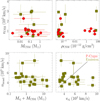 |
Fig. 11 Top-left: velocity of the CSM versus the CSM mass retrieved from the CSI modeling of 24 SNe Ibn of the MOSFiT sample. The velocity of the CSM is estimated either from the minimum of the absorption component of the P-Cygni profile (red circles) or the FWHM of the emission component (olive squares) of He I λ5876 Å line. Top-right: similar to to the top-left panel, showing the velocity of the CSM versus the CSM density. Bottom-left: broadest velocity component of the He I λ5876 Å line through the entire spectroscopic evolution versus the sum of the CSM and ejecta masses from MOSFiT CSI modeling. Bottom-right: similar to the bottom-left panel, showing the broadest velocity component of He I λ5876 Å line versus the ejecta velocity from MOSFiT CSI modeling. |
Data availability
Full Tables D.1, D.2, D.4, D.5, and D.7 are available at the CDS via https://cdsarc.cds.unistra.fr/viz-bin/cat/J/A+A/708/A270
The unpublished spectra of all SNe in the F25 sample (Table D.2) are now available in WISeREP via www.wiserep.org.
Acknowledgements
We thank Miika Pursiainen and Craig Pellegrino for supplying the spectra of SN 2023emq and SN 2022ablq, respectively. This work is supported by a VILLUM FONDEN Young Investigator Grant (project number 25501) a Villum Experiment grant (VIL69896) and by research grants (VIL16599, VIL54489) from VILLUM FONDEN. Parts of this research were supported by the Australian Research Council Centre of Excellence for Gravitational Wave Discovery (OzGrav), through project number CE230100016. The Villar Astro Time Lab acknowledges support through the David and Lucile Packard Foundation, National Science Foundation under AST-2433718, AST-2407922 and AST-2406110, as well as an Aramont Fellowship for Emerging Science Research. KdS thanks the LSST-DA Data Science Fellowship Program, which is funded by LSST-DA, the Brinson Foundation, the WoodNext Foundation, and the Research Corporation for Science Advancement Foundation; her participation in the program has benefited this work. This work is supported by the National Science Foundation under Cooperative Agreement PHY-2019786 (The NSF AI Institute for Artificial Intelligence and Fundamental Interactions, http://iaifi.org/). This material is based upon work supported by the National Science Foundation Graduate Research Fellowship Program under Grant Nos. 1842402 and 2236415. Any opinions, findings, conclusions, or recommendations expressed in this material are those of the authors and do not necessarily reflect the views of the National Science Foundation. D.O.J. acknowledges support from NSF grants AST-2407632 and AST-2429450, NASA grant 80NSSC24M0023, and HST/JWST grants HST-GO-17128.028, HST-GO-16269.012, and JWST-GO-05324.031, awarded by the Space Telescope Science Institute (STScI), which is operated by the Association of Universities for Research in Astronomy, Inc., for NASA, under contract NAS5-26555. G.N acknowledges NSF support from AST-2206195 for his involvement in this work. G.N is additionally funded by NSF CAREER grant AST-2239364, supported in-part by funding from Charles Simonyi, OAC-2311355, AST-2432428, as well as AST-2421845 and funding from the Simons Foundation for the NSF-Simons SkAI Institute. G.N is also supported by the DOE through the Department of Physics at the University of Illinois, Urbana-Champaign (# 13771275), and the HST Guest Observer Program through HST-GO-16764. and HST-GO-17128 (PI: R. Foley). W.J.-G. is supported by NASA through Hubble Fellowship grant HSTHF2-51558.001-A awarded by the Space Telescope Science Institute, which is operated for NASA by the Association of Universities for Research in Astronomy, Inc., under contract NAS5-26555. L.I acknowledges financial support from the INAF Data Grant Program ‘YES’ (PI: Izzo). C.D.K. gratefully acknowledges support from the NSF through AST-2432037, the HST Guest Observer Program through HST-SNAP-17070 and HST-GO-17706, and from JWST Archival Research through JWST-AR-6241 and JWST-AR-5441. We thank the Swope observers for their valuable contributions: Abdo Campillay, Yilin Kong Riveros and Jorge Anaís. M.R.S is supported by the STScI Postdoctoral Fellowship. Y.Z acknowledges visitor support from the Kavli Institute for Cosmology, Cambridge, where part of this work was completed. The data presented here were obtained in part with ALFOSC, which is provided by the Instituto de Astrofísica de Andalucía (IAA) under a joint agreement with the University of Copenhagen and NOT. Research at Lick Observatory is partially supported by a generous gift from Google. Based in part on observations obtained at the SOAR telescope, which is a joint project of the Ministério da Ciência, Tecnologia e Inovações (MCTI/LNA) do Brasil, the US National Science Foundation’s NOIRLab, the University of North Carolina at Chapel Hill (UNC), and Michigan State University (MSU). We acknowledge the use of public data from the Swift data archive. This work makes use of data taken with the Las Cumbres Observatory global telescope network. The LCO group is funded by NSF grants AST-1911151 and AST-1911225. This work has made use of data from the ATLAS project. ATLAS is primarily funded to search for near-Earth asteroids through NASA grants NN12AR55G, 80NSSC18K0284, and 80NSSC18K1575; byproducts of the NEO search include images and catalogs from the survey area. The ATLAS science products have been made possible through the contributions of the University of Hawaii Institute for Astronomy, the Queen’s University Belfast, and the Space Telescope Science Institute. YSE-PZ was developed by the UC Santa Cruz Transients Team. The UCSC team is supported in part by NASA grants NNG17PX03C, 80NSSC19K1386, and 80NSSC20K0953; NSF grants AST-1518052, AST-1815935, and AST-1911206; the Gordon & Betty Moore Foundation; the Heising-Simons Foundation; a fellowship from the David and Lucile Packard Foundation to R.J.F.; Gordon and Betty Moore Foundation postdoctoral fellowships and a NASA Einstein Fellowship, as administered through the NASA Hubble Fellowship program and grant HST-HF2-51462.001, to D.O.J.; and an NSF Graduate Research Fellowship, administered through grant DGE-1339067, to D.A.C.
References
- Aamer, A., Moore, T., Ramsden, P., et al. 2023, Transient Name Server Classification Report, 2023-2840, 1 [Google Scholar]
- Afsariardchi, N., Drout, M. R., Khatami, D. K., et al. 2021, ApJ, 918, 89 [NASA ADS] [CrossRef] [Google Scholar]
- Alam, S., Albareti, F. D., Allende Prieto, C., et al. 2015, ApJS, 219, 12 [Google Scholar]
- Aleo, P. D., Malanchev, K., Sharief, S., et al. 2022, arXiv e-prints [arXiv:2211.07128] [Google Scholar]
- Ambikasaran, S., Foreman-Mackey, D., Greengard, L., Hogg, D. W., & O’Neil, M. 2015, IEEE Trans. Pattern Anal. Mach. Intell., 38, 252 [Google Scholar]
- Angus, C. 2021, Transient Name Server Classification Report, 2021-1206, 1 [Google Scholar]
- Angus, C., Wiseman, P., Frohmaier, C., Swann, E., & Irani, I. 2019, Transient Name Server Classification Report, 2019-1390, 1 [Google Scholar]
- Anupama, G. C., Sahu, D. K., Gurugubelli, U. K., et al. 2009, MNRAS, 392, 894 [NASA ADS] [CrossRef] [Google Scholar]
- Arnett, & Fu, A. 1989, ApJ, 340, 396 [NASA ADS] [CrossRef] [Google Scholar]
- Baer-Way, R., Nayana, A. J., Jacobson-Galan, W., et al. 2025, arXiv e-prints [arXiv:2509.07080] [Google Scholar]
- Balcon, C. 2023, Transient Name Server Classification Report, 2023-2931, 1 [Google Scholar]
- Ben-Ami, T., Arcavi, I., Newsome, M., et al. 2023, ApJ, 946, 30 [NASA ADS] [CrossRef] [Google Scholar]
- Bersier, D. 2019, Transient Name Server Discovery Report, 2019-1317, 1 [Google Scholar]
- Brennan, S. J., Sollerman, J., Irani, I., et al. 2024, A&A, 684, L18 [NASA ADS] [CrossRef] [EDP Sciences] [Google Scholar]
- Brown, T. M., Baliber, N., Bianco, F. B., et al. 2013, PASP, 125, 1031 [Google Scholar]
- Burrows, D. N., Hill, J. E., Nousek, J. A., et al. 2005, SSR, 120, 165 [Google Scholar]
- Byrne, R. A., Fraser, M., Cai, Y.-Z., Reguitti, A., & Valerin, G. 2023, MNRAS, 524, 2978 [NASA ADS] [CrossRef] [Google Scholar]
- Carr, A., Davis, T. M., Camilleri, R., et al. 2024, PASA, 41, e068 [Google Scholar]
- Castro-Segura, N., Pursiainen, M., Smith, M., & Yaron, O. 2018, Transient Name Server Classification Report, 2018-2064, 1 [Google Scholar]
- Chambers, K. C., Magnier, E. A., Metcalfe, N., et al. 2016, arXiv e-prints [arXiv:1612.05560] [Google Scholar]
- Chambers, K. C., Boer, T. D., Bulger, J., et al. 2020, Transient Name Server Discovery Report, 2020-2783, 1 [Google Scholar]
- Chambers, K. C., Boer, T. D., Bulger, J., et al. 2022, Transient Name Server Discovery Report, 2022-2038, 1 [Google Scholar]
- Chandra, P., Chevalier, R. A., Chugai, N., et al. 2012, ApJ, 755, 110 [NASA ADS] [CrossRef] [Google Scholar]
- Chandra, P., Chevalier, R. A., Chugai, N., Fransson, C., & Soderberg, A. M. 2015, ApJ, 810, 32 [NASA ADS] [CrossRef] [Google Scholar]
- Charalampopoulos, P., Pursiainen, M., Onori, F., & Roy, R. 2023, Transient Name Server Classification Report, 2023-454, 1 [Google Scholar]
- Chatzopoulos, Wheeler, J. C., & Vinko, J. 2009, ApJ, 704, 1251 [Google Scholar]
- Chatzopoulos, E., Wheeler, J. C., & Vinko, J. 2012, ApJ, 746, 121 [Google Scholar]
- Chatzopoulos, E., Wheeler, J. C., Vinko, J., Horvath, Z. L., & Nagy, A. 2013, ApJ, 773, 76 [NASA ADS] [CrossRef] [Google Scholar]
- Chevalier, R. A., & Irwin, C. M. 2011, ApJ, 729, L6 [Google Scholar]
- Chevalier, R. A., & Fransson, C. 2017, Thermal and Non-thermal Emission from Circumstellar Interaction, eds. A. W. Alsabti, & P. Murdin (Cham: Springer International Publishing), 875 [Google Scholar]
- Childress, M. J., Vogt, F. P. A., Nielsen, J., & Sharp, R. G. 2014, Ap&SS, 349, 617 [Google Scholar]
- Chu, M., Dahiwale, A., & Fremling, C. 2021, Transient Name Server Classification Report, 2021-3105, 1 [Google Scholar]
- Clemens, J. C., Crain, J. A., & Anderson, R. 2004, in Ground-based Instrumentation for Astronomy, 5492, eds. A. F. M. Moorwood, & M. Iye, International Society for Optics and Photonics (SPIE), 331 [Google Scholar]
- Colgate, S. A., & McKee, C. 1969, ApJ, 157, 623 [NASA ADS] [CrossRef] [Google Scholar]
- Corder, G., & Foreman, D. 2014, Nonparametric Statistics: A Step-by-Step Approach (Wiley) [Google Scholar]
- Coulter, D. A., Jones, D. O., McGill, P., et al. 2023, PASP, 135, 064501 [Google Scholar]
- Curran, P. A. 2014, arXiv e-prints [arXiv:1411.3816] [Google Scholar]
- Davis, K., Jacobson-Galan, W., & Foley, R. 2023a, Transient Name Server Classification Report, 2023-2148, 1 [Google Scholar]
- Davis, K. W., Taggart, K., Tinyanont, S., et al. 2023b, MNRAS, 523, 2530 [NASA ADS] [CrossRef] [Google Scholar]
- Desai, D. 2023, Transient Name Server Classification Report, 2023-2842, 1 [Google Scholar]
- Dessart, L. 2024, arXiv e-prints [arXiv:2405.04259] [Google Scholar]
- Dessart, L., Audit, E., & Hillier, D. J. 2015, MNRAS, 449, 4304 [Google Scholar]
- Dessart, L., Hillier, D. J., & Kuncarayakti, H. 2022, A&A, 658, A130 [NASA ADS] [CrossRef] [EDP Sciences] [Google Scholar]
- Dong, Y., Tsuna, D., Valenti, S., et al. 2024, arXiv e-prints [arXiv:2405.04583] [Google Scholar]
- Dopita, M., Hart, J., McGregor, P., et al. 2007, Ap&SS, 310, 255 [Google Scholar]
- Dugas, A., Fremling, C., & Sharma, Y. 2019, Transient Name Server Classification Report, 2019-2841, 1 [Google Scholar]
- Dwarkadas, V. V., & Gruszko, J. 2012, MNRAS, 419, 1515 [Google Scholar]
- Dwarkadas, V. V., Romero-Cañizales, C., Reddy, R., & Bauer, F. E. 2016, MNRAS, 462, 1101 [Google Scholar]
- Ercolino, A., Jin, H., Langer, N., & Dessart, L. 2024, arXiv e-prints [arXiv:2412.09893] [Google Scholar]
- Farias, D., Gall, C., Narayan, G., et al. 2024, ApJ, 977, 152 [Google Scholar]
- Fassia, A., Meikle, W. P. S., Chugai, N., et al. 2001, MNRAS, 325, 907 [NASA ADS] [CrossRef] [Google Scholar]
- Filippenko, A. V. 1997, ARA&A, 35, 309 [Google Scholar]
- Fitzpatrick, E. L. 2004, in Astronomical Society of the Pacific Conference Series, 309, Astrophysics of Dust, eds. A. N. Witt, G. C. Clayton, & B. T. Draine, 33 [Google Scholar]
- Flewelling, H. A., Magnier, E. A., Chambers, K. C., et al. 2020, ApJS, 251, 7 [NASA ADS] [CrossRef] [Google Scholar]
- Foley, R. J., Papenkova, M. S., Swift, B. J., et al. 2003, PASP, 115, 1220 [NASA ADS] [CrossRef] [Google Scholar]
- Foley, R. J., Smith, N., Ganeshalingam, M., et al. 2007, ApJ, 657, L105 [NASA ADS] [CrossRef] [Google Scholar]
- Foreman-Mackey, D., Hogg, D. W., Lang, D., & Goodman, J. 2013, PASP, 125, 306 [Google Scholar]
- Fransson, C., Ergon, M., Challis, P. J., et al. 2014, ApJ, 797, 118 [Google Scholar]
- Fransson, C., Lundqvist, P., & Chevalier, R. A. 1996, ApJ, 461, 993 [NASA ADS] [CrossRef] [Google Scholar]
- Fraser, M. 2020, Roy. Soc. Open Sci., 7, 200467 [NASA ADS] [CrossRef] [Google Scholar]
- Fraser, M., Stritzinger, M. D., Brennan, S. J., et al. 2021, arXiv e-prints [arXiv:2108.07278] [Google Scholar]
- Fremling, C. 2021, Transient Name Server Discovery Report, 2021-2918, 1 [Google Scholar]
- Fremling, C. 2022, Transient Name Server Discovery Report, 2022-167, 1 [Google Scholar]
- Fremling, C. 2023a, Transient Name Server Discovery Report, 2023-2074, 1 [Google Scholar]
- Fremling, C. 2023b, Transient Name Server Discovery Report, 2023-2126, 1 [Google Scholar]
- Fremling, C. 2023c, Transient Name Server Discovery Report, 2023-2744, 1 [Google Scholar]
- Fremling, C. 2023d, Transient Name Server Discovery Report, 2023-2892, 1 [Google Scholar]
- Fulton, M., Bulger, J., Huber, M. E., et al. 2022a, Transient Name Server Classification Report, 2022-2789, 1 [Google Scholar]
- Fulton, M., Srivastav, S., Smartt, S. J., et al. 2022b, Transient Name Server Classification Report, 2022-455, 1 [Google Scholar]
- Fulton, M., Srivastav, S., Smith, K. W., et al. 2022c, Transient Name Server Classification Report, 2022-3486, 1 [Google Scholar]
- Fulton, M., Srivastav, S., Smith, K. W., et al. 2022d, Transient Name Server Classification Report, 2022-3522, 1 [Google Scholar]
- Gal-Yam, A., Bruch, R., Schulze, S., et al. 2022, Nature, 601, 201 [NASA ADS] [CrossRef] [Google Scholar]
- Gangopadhyay, A., Misra, K., Hiramatsu, D., et al. 2020, ApJ, 889, 170 [NASA ADS] [CrossRef] [Google Scholar]
- Gangopadhyay, A., Misra, K., Hosseinzadeh, G., et al. 2022, ApJ, 930, 127 [NASA ADS] [CrossRef] [Google Scholar]
- Gangopadhyay, A., Dukiya, N., Moriya, T. J., et al. 2025, MNRAS, 537, 2898 [Google Scholar]
- Gangopadhyay, A., Sollerman, J., Tsalapatas, K., et al. 2025, MNRAS, accepted [arXiv:2506.10700] [Google Scholar]
- Gorbikov, E., Gal-Yam, A., Ofek, E. O., et al. 2014, MNRAS, 443, 671 [NASA ADS] [CrossRef] [Google Scholar]
- Gordon, K. 2024, J. Open Source Softw., 9, 7023 [NASA ADS] [CrossRef] [Google Scholar]
- Graham, M. L., Dahiwale, A., & Fremling, C. 2020, Transient Name Server Classification Report, 2020-2927, 1 [Google Scholar]
- Guillochon, J., Nicholl, M., Villar, V. A., et al. 2018, ApJS, 236, 6 [NASA ADS] [CrossRef] [Google Scholar]
- Hamers, A. S., & Dosopoulou, F. 2019, ApJ, 872, 119 [NASA ADS] [CrossRef] [Google Scholar]
- HI4PI Collaboration (Ben Bekhti, N., et al.) 2016, A&A, 594, A116 [NASA ADS] [CrossRef] [EDP Sciences] [Google Scholar]
- Hinds, K., Perley, D., & Irani, I. 2023, Transient Name Server Discovery Report, 2023-1152, 1 [Google Scholar]
- Hinkle, J. 2023, Transient Name Server Classification Report, 2023-2507, 1 [Google Scholar]
- Hiramatsu, D., Hosseinzadeh, G., Burke, J., et al. 2020, Transient Name Server Classification Report, 2020-3728, 1 [Google Scholar]
- Hiramatsu, D., Matsumoto, T., Berger, E., et al. 2024, ApJ, 964, 181 [Google Scholar]
- Ho, A. Y. Q., Perley, D. A., Gal-Yam, A., et al. 2021, arXiv e-prints [arXiv:2105.08811] [Google Scholar]
- Hodgkin, S. T., Breedt, E., Delgado, A., et al. 2023, Transient Name Server Discovery Report, 2023-3352, 1 [Google Scholar]
- Horne, K. 1986, PASP, 98, 609 [Google Scholar]
- Hosseinzadeh, G., Arcavi, I., Valenti, S., et al. 2017, ApJ, 836, 158 [Google Scholar]
- Hosseinzadeh, G., Sand, D. J., Williamson, M., et al. 2022, Transient Name Server Classification Report, 2022-2316, 1 [Google Scholar]
- Huber, M., Chambers, K. C., Flewelling, H., et al. 2015, Astronomer’s Telegram, 7153 [Google Scholar]
- Immler, S., Modjaz, M., Landsman, W., et al. 2008, ApJ, 674, L85 [Google Scholar]
- Inoue, Y., & Maeda, K. 2024, arXiv e-prints [arXiv:2412.09066] [Google Scholar]
- Jacobson-Galan, W. 2021, Transient Name Server Classification Report, 2021-3666, 1 [Google Scholar]
- Jacobson-Galán, W. 2022, Transient Name Server Classification Report, 2022-1161, 1 [Google Scholar]
- Jacobson-Galán, W. 2025, Transient Name Server AstroNote, 21, 1 [Google Scholar]
- Jacobson-Galán, W., Gillanders, J., Smartt, S. J., et al. 2024a, Transient Name Server Classification Report, 2024-22, 1 [Google Scholar]
- Jacobson-Galán, W. V., Dessart, L., Davis, K. W., et al. 2024b, ApJ, 970, 189 [CrossRef] [Google Scholar]
- Jones, D. O., Foley, R. J., Narayan, G., et al. 2021a, ApJ, 908, 143 [NASA ADS] [CrossRef] [Google Scholar]
- Jones, D. O., French, K. D., Agnello, A., et al. 2021b, Transient Name Server Discovery Report, 2021-1145, 1 [Google Scholar]
- Jones, D. O., French, K. D., Agnello, A., et al. 2021c, Transient Name Server Discovery Report, 2021-3267, 1 [Google Scholar]
- Karamehmetoglu, E., Taddia, F., Sollerman, J., et al. 2017, A&A, 602, A93 [NASA ADS] [CrossRef] [EDP Sciences] [Google Scholar]
- Karamehmetoglu, E., Fransson, C., Sollerman, J., et al. 2021, A&A, 649, A163 [NASA ADS] [CrossRef] [EDP Sciences] [Google Scholar]
- Khakpash, S., Bianco, F. B., Modjaz, M., et al. 2024, ApJS, 275, 37 [Google Scholar]
- Khazov, D., Yaron, O., Gal-Yam, A., et al. 2016, ApJ, 818, 3 [CrossRef] [Google Scholar]
- Kilpatrick, C. D., Foley, R. J., Drout, M. R., et al. 2018, MNRAS, 473, 4805 [NASA ADS] [CrossRef] [Google Scholar]
- Kool, E. C., Karamehmetoglu, E., Sollerman, J., et al. 2021, A&A, 652, A136 [NASA ADS] [CrossRef] [EDP Sciences] [Google Scholar]
- Kool, E., Chu, M., Dahiwale, A., & Fremling, C. 2022, Transient Name Server Classification Report, 2022-1122, 1 [Google Scholar]
- Labrie, K., Anderson, K., Cárdenes, R., Simpson, C., & Turner, J. E. H. 2019, in Astronomical Society of the Pacific Conference Series, 523, Astronomical Data Analysis Software and Systems XXVII, eds. P. J. Teuben, M. W. Pound, B. A. Thomas, & E. M. Warner, 321 [Google Scholar]
- Lantz, B., Aldering, G., Antilogus, P., et al. 2004, SPIE Conf. Ser., 5249, 146 [Google Scholar]
- Li, L., Lin, H., Zhai, Q., et al. 2023, Transient Name Server Classification Report, 2023-1163, 1 [Google Scholar]
- Liu, Y.-Q., Modjaz, M., Bianco, F. B., & Graur, O. 2016, ApJ, 827, 90 [NASA ADS] [CrossRef] [Google Scholar]
- Lu, W., Fuller, J., Quataert, E., & Bonnerot, C. 2023, MNRAS, 519, 1409 [Google Scholar]
- Maeda, K., & Moriya, T. J. 2022, ApJ, 927, 25 [NASA ADS] [CrossRef] [Google Scholar]
- Magnier, E. A., Chambers, K. C., Flewelling, H. A., et al. 2020, ApJS, 251, 3 [NASA ADS] [CrossRef] [Google Scholar]
- Margalit, B., Quataert, E., & Ho, A. Y. Q. 2022, ApJ, 928, 122 [Google Scholar]
- Marques-Chaves, R., Perez-Fournon, I., Angel, C. J., et al. 2022, Transient Name Server Discovery Report, 2022-1065, 1 [Google Scholar]
- Massey, P. 1981, ApJ, 246, 153 [NASA ADS] [CrossRef] [Google Scholar]
- Matheson, T., Filippenko, A. V., Chornock, R., Leonard, D. C., & Li, W. 2000, AJ, 119, 2303 [NASA ADS] [CrossRef] [Google Scholar]
- Matzner, C. D., & McKee, C. F. 1999, ApJ, 510, 379 [Google Scholar]
- Maund, J. R., Pastorello, A., Mattila, S., Itagaki, K., & Boles, T. 2016, ApJ, 833, 128 [NASA ADS] [CrossRef] [Google Scholar]
- McCully, C., Volgenau, N. H., Harbeck, D.-R., et al. 2018, SPIE Conf. Ser., 10707, 107070K [Google Scholar]
- Meza, N., & Anderson, J. P. 2020, A&A, 641, A177 [NASA ADS] [CrossRef] [EDP Sciences] [Google Scholar]
- Miller, J. S., & Stone, R. P. S. 1993, Lick Obs. Tech. Rep. 66 (Santa Cruz: Lick Obs). [Google Scholar]
- Moriya, T. J., & Maeda, K. 2016, ApJ, 824, 100 [Google Scholar]
- Munoz-Arancibia, A., Bauer, F. E., Forster, F., et al. 2022, Transient Name Server Discovery Report, 2022-914, 1 [Google Scholar]
- Nymark, T. K., Chandra, P., & Fransson, C. 2009, A&A, 494, 179 [NASA ADS] [CrossRef] [EDP Sciences] [Google Scholar]
- Oke, J. B., Cohen, J. G., Carr, M., et al. 1995, PASP, 107, 375 [Google Scholar]
- Panjkov, S., Auchettl, K., Shappee, B. J., et al. 2024, PASA, 41, e059 [Google Scholar]
- Pastorello, A., Smartt, S. J., Mattila, S., et al. 2007, Nature, 447, 829 [NASA ADS] [CrossRef] [Google Scholar]
- Pastorello, A., Quimby, R. M., Smartt, S. J., et al. 2008a, MNRAS, 389, 131 [NASA ADS] [CrossRef] [Google Scholar]
- Pastorello, A., Mattila, S., Zampieri, L., et al. 2008b, MNRAS, 389, 113 [Google Scholar]
- Pastorello, A., Benetti, S., Brown, P. J., et al. 2015a, MNRAS, 449, 1921 [Google Scholar]
- Pastorello, A., Hadjiyska, E., Rabinowitz, D., et al. 2015b, MNRAS, 449, 1954 [Google Scholar]
- Pastorello, A., Prieto, J. L., Elias-Rosa, N., et al. 2015c, MNRAS, 453, 3649 [Google Scholar]
- Pastorello, A., Tartaglia, L., Elias-Rosa, N., et al. 2015d, MNRAS, 454, 4293 [Google Scholar]
- Pastorello, A., Wyrzykowski, Ł., Valenti, S., et al. 2015e, MNRAS, 449, 1941 [NASA ADS] [CrossRef] [Google Scholar]
- Pastorello, A., Wang, X. F., Ciabattari, F., et al. 2016, MNRAS, 456, 853 [Google Scholar]
- Payne, A. V. 2022, Transient Name Server Classification Report, 2022-728, 1 [Google Scholar]
- Pellegrino, C., Gonzalez, E. P., Farah, J., et al. 2023a, Transient Name Server Classification Report, 2023-725, 1 [Google Scholar]
- Pellegrino, C., Hosseinzadeh, G., Farah, J., et al. 2023b, Transient Name Server Classification Report, 2023-1279, 1 [Google Scholar]
- Pellegrino, C., Howell, D. A., Terreran, G., et al. 2022a, ApJ, 938, 73 [NASA ADS] [CrossRef] [Google Scholar]
- Pellegrino, C., Howell, D. A., Vinkó, J., et al. 2022b, ApJ, 926, 125 [NASA ADS] [CrossRef] [Google Scholar]
- Pellegrino, C., Li, W., Burke, J., et al. 2022c, Transient Name Server Classification Report, 2022-1082, 1 [Google Scholar]
- Pellegrino, C., Terreran, G., Burke, J., et al. 2022d, Transient Name Server Classification Report, 2022-754, 1 [Google Scholar]
- Pellegrino, C., Modjaz, M., Takei, Y., et al. 2024, ApJ, 977, 2 [Google Scholar]
- Perley, D. A., Sollerman, J., Schulze, S., et al. 2022, ApJ, 927, 180 [NASA ADS] [CrossRef] [Google Scholar]
- Planck Collaboration XVI. 2014, A&A, 571, A16 [NASA ADS] [CrossRef] [EDP Sciences] [Google Scholar]
- Poznanski, D., Prochaska, J. X., & Bloom, J. S. 2012, MNRAS, 426, 1465 [Google Scholar]
- Privon, G. C., Ricci, C., Aalto, S., et al. 2020, ApJ, 893, 149 [NASA ADS] [CrossRef] [Google Scholar]
- Pursiainen, M., Leloudas, G., Schulze, S., et al. 2023, ApJ, 959, L10 [NASA ADS] [CrossRef] [Google Scholar]
- Ransome, C. L., & Villar, V. A. 2024, arXiv e-prints [arXiv:2409.10596] [Google Scholar]
- Rasmussen, C., & Williams, C. 2005, Gaussian Processes for Machine Learning, Adaptive Computation And Machine Learning (MIT Press) [Google Scholar]
- Rest, A., Stubbs, C., Becker, A. C., et al. 2005, ApJ, 634, 1103 [NASA ADS] [CrossRef] [Google Scholar]
- Rest, A., Scolnic, D., Foley, R. J., et al. 2014, ApJ, 795, 44 [Google Scholar]
- Rest, S., Rest, A., Kilpatrick, C. D., et al. 2024, arXiv e-prints [arXiv:2405.03747] [Google Scholar]
- Rockosi, C., Stover, R., Kibrick, R., et al. 2010, SPIE Conf. Ser., 7735, 77350R [Google Scholar]
- Rodríguez, Ó., Maoz, D., & Nakar, E. 2023, ApJ, 955, 71 [CrossRef] [Google Scholar]
- Roming, P. W. A., Kennedy, T. E., Mason, K. O., et al. 2005, Space Sci. Rev., 120, 95 [Google Scholar]
- Sanders, N. E., Soderberg, A. M., Foley, R. J., et al. 2013, ApJ, 769, 39 [Google Scholar]
- Sarin, N., Hübner, M., Omand, C. M. B., et al. 2024, MNRAS, 531, 1203 [NASA ADS] [CrossRef] [Google Scholar]
- Schechter, P. L., Mateo, M., & Saha, A. 1993, PASP, 105, 1342 [Google Scholar]
- Schlafly, E. F., & Finkbeiner, D. P. 2011, ApJ, 737, 103 [Google Scholar]
- Shivvers, I., Zheng, W. K., Mauerhan, J., et al. 2016, MNRAS, 461, 3057 [Google Scholar]
- Shivvers, I., Zheng, W., Van Dyk, S. D., et al. 2017, MNRAS, 471, 4381 [Google Scholar]
- Siebert, M. R., Foley, R. J., Jones, D. O., et al. 2019, MNRAS, 486, 5785 [CrossRef] [Google Scholar]
- Siebert, M. R., Tinyanont, S., Taggart, K., & Foley, R. J. 2021, Transient Name Server Classification Report, 2021-1615, 1 [Google Scholar]
- Silverman, J. M., Ganeshalingam, M., Li, W., & Filippenko, A. V. 2012, MNRAS, 425, 1889 [Google Scholar]
- Smartt, S. J., Chambers, K. C., Smith, K. W., et al. 2016, ApJ, 827, L40 [Google Scholar]
- Smith, N. 2014, ARA&A, 52, 487 [Google Scholar]
- Smith, N., Mauerhan, J. C., Silverman, J. M., et al. 2012, MNRAS, 426, 1905 [NASA ADS] [CrossRef] [Google Scholar]
- Smith, K. W., Williams, R. D., Young, D. R., et al. 2019, RNAAS, 3, 26 [NASA ADS] [Google Scholar]
- Sollerman, J., Chu, M., Dahiwale, A., & Fremling, C. 2023, Transient Name Server Classification Report, 2023-3181, 1 [Google Scholar]
- Speagle, J. S. 2020, MNRAS, 493, 3132 [Google Scholar]
- Spearman, C. 1904, Am. J. Psychol., 15, 72 [Google Scholar]
- Srivastav, S., Smartt, S. J., McBrien, O., et al. 2020, Transient Name Server Classification Report, 2020-2148, 1 [Google Scholar]
- Stanek, K. Z. 2022, Transient Name Server Discovery Report, 2022-3421, 1 [Google Scholar]
- Stevance, H. F., & Lee, A. 2023, MNRAS, 518, 5741 [Google Scholar]
- Stritzinger, M. D., Taddia, F., Burns, C. R., et al. 2018, A&A, 609, A135 [NASA ADS] [CrossRef] [EDP Sciences] [Google Scholar]
- Strotjohann, N. L., Ofek, E. O., Gal-Yam, A., et al. 2021, ApJ, 907, 99 [NASA ADS] [CrossRef] [Google Scholar]
- Sun, N.-C., Maund, J. R., Hirai, R., Crowther, P. A., & Podsiadlowski, P. 2020, MNRAS, 491, 6000 [NASA ADS] [CrossRef] [Google Scholar]
- Suzuki, A., Moriya, T. J., & Takiwaki, T. 2019, ApJ, 887, 249 [Google Scholar]
- Swift, J. J., Andersen, K., Arculli, T., et al. 2022, PASP, 134, 035005 [Google Scholar]
- Taddia, F., Stritzinger, M. D., Bersten, M., et al. 2018, A&A, 609, A136 [NASA ADS] [CrossRef] [EDP Sciences] [Google Scholar]
- Taguchi, K., Singh, A., Kawabata, M., Maeda, K., & Gangopadhyay, A. 2023, Transient Name Server Classification Report, 2023-2735, 1 [Google Scholar]
- Takei, Y., Tsuna, D., Ko, T., & Shigeyama, T. 2024, ApJ, 961, 67 [Google Scholar]
- Tonry, J. L., Denneau, L., Heinze, A. N., et al. 2018, PASP, 130, 064505 [Google Scholar]
- Tonry, J., Denneau, L., Heinze, A., et al. 2020a, Transient Name Server Discovery Report, 2020-2022, 1 [Google Scholar]
- Tonry, J., Denneau, L., Heinze, A., et al. 2020b, Transient Name Server Discovery Report, 2020-3630, 1 [Google Scholar]
- Tonry, J., Denneau, L., Weiland, H., et al. 2022a, Transient Name Server Discovery Report, 2022-716, 1 [Google Scholar]
- Tonry, J., Denneau, L., Weiland, H., et al. 2022b, Transient Name Server Discovery Report, 2022-2180, 1 [Google Scholar]
- Tonry, J., Denneau, L., Weiland, H., et al. 2023a, Transient Name Server Discovery Report, 2023-698, 1 [Google Scholar]
- Tonry, J., Denneau, L., Weiland, H., et al. 2023b, Transient Name Server Discovery Report, 2023-2485, 1 [Google Scholar]
- Tsuna, D., Matsumoto, T., Wu, S. C., & Fuller, J. 2024a, ApJ, 966, 30 [Google Scholar]
- Tsuna, D., Wu, S. C., Fuller, J., Dong, Y., & Piro, A. L. 2024b, Open J. Astrophys., 7, 82 [Google Scholar]
- Tucker, M. A. 2023, Transient Name Server Classification Report, 2023-2118, 1 [Google Scholar]
- Tucker, M. A., Shappee, B. J., Huber, M. E., et al. 2022, PASP, 134, 124502 [NASA ADS] [CrossRef] [Google Scholar]
- Turatto, M., Benetti, S., & Cappellaro, E. 2003, in From Twilight to Highlight: The Physics of Supernovae, eds. W. Hillebrandt & B. Leibundgut (Berlin, Heidelberg: Springer Berlin Heidelberg), 200 [Google Scholar]
- Vallely, P. J., Prieto, J. L., Stanek, K. Z., et al. 2018, MNRAS, 475, 2344 [NASA ADS] [CrossRef] [Google Scholar]
- Vallely, P. J., Kochanek, C. S., Stanek, K. Z., Fausnaugh, M., & Shappee, B. J. 2021, MNRAS, 500, 5639 [Google Scholar]
- Villar, V. A., Berger, E., Metzger, B. D., & Guillochon, J. 2017, ApJ, 849, 70 [NASA ADS] [CrossRef] [Google Scholar]
- Virtanen, P., Gommers, R., Oliphant, T. E., et al. 2020, Nat. Methods, 17, 261 [Google Scholar]
- Wang, S.-Q., & Li, L. 2020, ApJ, 900, 83 [Google Scholar]
- Wang, X., Lin, W., Zhang, J., et al. 2021, ApJ, 917, 97 [NASA ADS] [CrossRef] [Google Scholar]
- Wang, Q., Goel, A., Dessart, L., et al. 2024a, MNRAS, 530, 3906 [NASA ADS] [CrossRef] [Google Scholar]
- Wang, Z., Pastorello, A., Maeda, K., et al. 2024b, A&A, 691, A156 [NASA ADS] [CrossRef] [EDP Sciences] [Google Scholar]
- Wang, Z. Y., Pastorello, A., Maeda, K., et al. 2024c, VizieR On-line Data Catalog: J/A+A/ 691/A156. Originally published in: 2024A&A...691A.156W [Google Scholar]
- Wang, Z.-Y., Pastorello, A., Cai, Y.-Z., et al. 2025, A&A, 700, A156 [NASA ADS] [CrossRef] [EDP Sciences] [Google Scholar]
- Warwick, B., Lyman, J., Pursiainen, M., et al. 2024, arXiv e-prints [arXiv:2409.14147] [Google Scholar]
- Waskom, M. L. 2021, J. Open Source Softw., 6, 3021 [CrossRef] [Google Scholar]
- Wu, S. C., & Fuller, J. 2022, ApJ, 940, L27 [NASA ADS] [CrossRef] [Google Scholar]
- Zhang, M., Gao, X., Sun, G., et al. 2023, Transient Name Server Discovery Report, 2023-2566, 1 [Google Scholar]
Appendix A About the host galaxy extinction
The method described in Sect. 3.3 to estimate the host galaxy extinction for SNe in the F25 sample is purely based on the SED construction at maximum light using the available photometric observations (see Fig. A.1). This approach might differ from the extinction values obtained by other methods, such as empirical relations between the equivalent widths of Na I D spectral lines and the color excess (Turatto et al. 2003; Poznanski et al. 2012). Unfortunately, for the latter, we require mediumresolution spectra to identify and measure the EWs of such lines, if present.
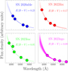 |
Fig. A.1 Collection of the SED (fλ versus wavelength) fitting of the interpolated light curves at maximum light of four SNe Ibn in the F25 sample. The fitting function is a modified blackbody, as described in Sect. 3.3. The values of the color excess reported in each plot were obtained assuming RV = 3.1. |
In order to exemplify the challenges in measuring the NaI D with the spectra of the SNe in the F25 sample, we take the most-extinguished SNe using the SED approach (E(B − V) > 0.2 mag), SNe 20191sm, 2020able, and 2021wvg, and check for the presence of such lines. Using the empirical relation in Turatto et al. (2003), the EWs of these lines should be ≳ 1.5 Å. The top panels of Fig. A.2 show the spectral region surrounding the Na I D lines, alongside the background regions to estimate a linear, local continuum. For all these SNe (and the rest of the SNe in the F25 sample), the Na I D lines lie on top of the red wing of a complex, strong He I λ5876 Å line. Additionally, the low spectral resolution and/or dispersion of the instrument and poor S/N in some cases leaves the Na absorption unresolved and poorly detected, as seen for SNe 2020able and 20191sm. To alleviate resolution-related issues, we linearly interpolated the spectra in 0.2 Å steps to better estimate the local continuum. With this approach, we normalized the region containing the Na I D lines by the continuum (bottom panels in Fig. A.2). For SNe 2020able and 2019lsm, we identified an absorption feature close to Na I D lines. The total EWs of the absorption trough of both SNe are ≈ 0.7 Å. For SN 2021wvg, no sodium absorption feature can be identified.
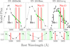 |
Fig. A.2 Top: Spectral region surrounding the potential Na I D lines (red, vertical lines) in the spectra of SNe 2020able (left), 20191sm (middle), and 2021wvg (right). Transparent, lime regions correspond to the background to estimate the local, linear continuum (lime, solid line). The location of the He I λ5876 Å is also shown in the panels. Bottom: Zoom-in on the normalized-by-continuum spectral regions presented in at the top. |
In summary, the discrepancies between the host galaxy extinction estimates from the SED method and those from the Na I D lines are large (half the expected value). However, since none of these methods provide accurate extinction measurements, only an estimation of the host galaxy extinction can be made. Nevertheless, all the results and conclusions in this work regarding SNe Ibn are only weakly dependent on these estimates, as they are drawn on a much larger sample than F25.
Appendix B Degeneracy of the MOSFiT parameters
To investigate a possible degeneracy of R0 and ρCSM obtained with MOSFiT, we show in Fig. B.1 the MOSFiT fits to the LC data of SN 2023iuc, which is the only SN that drastically changes ρCSM for each prior (A and B) and model selection (CSI and RD+CSI) in Sect. 4.2. The same trend is observed for several SNe that show discrepant CSM densities under different prior/models, such as SNe 2019deh, 2022ihx, 2020bqj, and 2019kbj, among others (Tables D.4 and D.5).
First, for SN 2023iuc, we note that the values of ρCSM resulting from different combinations of MOSFiT models and prior selection span from 2 × 10⁻¹⁸ to 2 × 10⁻⁹ g/cm3 (Fig. B.1). Second, the median values of MNi for the model RD+CSI and PRIOR A and RD+CSI and PRIOR B are ~0.001 and ~0.0001 M⊙, respectively. If these low nickel masses are true, then the CSM densities for any model setup should be next to identical. This is clearly not the case for SN 2023iuc since the differences span several orders of magnitude. Furthermore, there are also no significant differences in the resulting MOSFiT fits, visually and statistically, that might aid to prefer one model (or prior distribution) over the other. This points to a degeneracy of the models (or the way the CSM interaction is modeled) instead of a physical origin. These findings highlight the necessity to carefully choose the prior and models in any fitting procedure, and be cautious in interpreting the results.
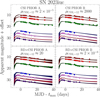 |
Fig. B.1 MOSFiT fits to the light curves of SN 2023iuc for the following combination of prior and models: PRIOR A CSI (top-left), PRIOR B CSI (top-right), PRIOR A RD+CSI (bottom-left) and PRIOR B RD+CSI (bottom-right). Within each panel, from bottom to top, the indigo, pink, violet, blue, green, red, and brown circles and curves correspond to photometric observations and fits in UVM2, UVW2, UVW1, up, gp, rp, and ip bands. Each panel contains the value of ρCSM (in units of 10−12 g/cm3) obtained from MOSFiT under the corresponding model and prior selection. |
Appendix C Figures
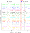 |
Fig. C.1 Left: Collection of the continuum-subtracted spectral region surrounding He I λ5876 Å of SNe in the F25 sample (Fλ versus wavelength). Right: Same as the left panel, but highlighting the Hα spectral region instead. |
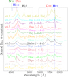 |
Fig. C.2 Collection of all 15 SNe Ibn that shows flash-ionized features (Fλ versus wavelength). For comparison, we include the Type IIn 1998S. Nine (from SN 20191sm to bottom) are first reported in this work. |
Appendix D Tables
Photometric data of Type Ibn SNe in the F25 sample.□
Log of spectroscopic observations of Type Ibn SNe in the F25 sample□.
Summary of Type Ibn SNe in the F25 sample.
Inferred values of the parameters of the CSI model for Type Ibn SNe in the MOSFiT sample.□,⋆
Inferred values of the parameters of the RD+CSI model for Type Ibn SNe in the MOSFiT sample.□,⋆
Results from the X-ray analysis of Type Ibn SNe in the X-RAY sample.
Minimum and maximum velocity* of the narrow and broad components of He I λ5876 Å line of 59 SNe Ibn.□
Photometric properties of our F25 + Literature sample of 61 SNe Ibn⋆.
All Tables
Inferred values of the parameters of the CSI model for Type Ibn SNe in the MOSFiT sample.□,⋆
Inferred values of the parameters of the RD+CSI model for Type Ibn SNe in the MOSFiT sample.□,⋆
Minimum and maximum velocity* of the narrow and broad components of He I λ5876 Å line of 59 SNe Ibn.□
All Figures
|
Fig. 1 Visualization of the four different SN Ibn samples (F25, X-RAY, MOSFiT, and Lit) analyzed in this work, with the individual member SN labeled. For details, see Tables D.8 and Table D.7b. |
| In the text | |
|
Fig. 2 Interpolated B − V (top) and g − r (bottom) curves for the 24 SNe Ibn from F25 (magenta filled circles), the Icn/Ibn (2023emq-like: yellow filled circles) and the color curves (±1σ) of the Lit sample (blue regions). The color curves (±1σ) of five SNe Icn are included for comparison (red regions). The photometric data of the SNe Icn were retrieved from Gal-Yam et al. (2022); Perley et al. (2022); Fraser et al. (2021); Pellegrino et al. (2022a); Davis et al. (2023b). |
| In the text | |
|
Fig. 3 Top: absolute R/r-band-like light curves of all SNe Ibn from F25 sample that are first reported in this work (magenta dots) and Lit sample (blue lines). Gray (H17) regions correspond to the average light curve and 1.96σ error bars of 18 Type Ibn SNe from Hosseinzadeh et al. (2017). Yellow dots correspond to the likely Icn/Ibn SNe 2023emq (Pursiainen et al. 2023), 2023qre, 2023rau and 2023xgo (this work). Red lines correspond to the five Icn SNe discovered up to date. Bottom: same as the top panel, with the subtraction of the peak magnitude of each SN. Green (K24) regions correspond to the median light curve and the 25% and 75% percentiles from Khakpash et al. (2024). |
| In the text | |
|
Fig. 4 Left: kernel density estimate (KDE) of the difference between the magnitude of the H17 R/r-band template and the magnitude of the SNe Ibn in the total sample of this work (61) normalized by the uncertainty of the H17 template, in 10-day bins. The white dots correspond to the median of each KDE, while the black solid bars the interquartile range, i.e., the 25% and 75% percentiles. Right: same as left panel, for the normalized H17 (nH17) template. |
| In the text | |
|
Fig. 5 Absolute (R/r-band) peak magnitude versus the absolute value of the slope parameters of the (R/r-band) light curves (γ). The SNe Ibn from the F25 and Lit samples are presented as magenta and blue circles, respectively. The top-left, top-right, and bottom-right panels show the light curve slopes γ−10 (−10 to tmax), γ+10 (tmax to day +10), γ+20 (+10 to +20 days), and γ+30 (+20 to +30 days), respectively. |
| In the text | |
|
Fig. 6 Absolute values of the R/r-band slopes γ−10 (left panel) and γ+20 (right panel) versus γ+10. The numbers within each plot are the Spearman’s coefficients and p-values for γ−10 versus γ+10 (left) and for γ+20 versus γ+10 (right). The SNe Ibn from the F25 and Lit samples are presented as magenta and blue circles, respectively. |
| In the text | |
|
Fig. 7 Inferred values of seven MOSFiT parameters for all 24 SNe in the MOSFiT sample. The parameters shown here are log Mej, vej, log MCSM, log ρCSM, with ρCSM in units of 10−12 g/cm3, log R0, with R0 in units of 1014 cm, s, n, and texp for the CSI (circle) and RD+CSI (square) models. The blue circle in each plot highlights the Type Ibn OGLE-2014-SN-131. For the CSI sample, the lime and crimson circles correspond to the SNe with ρCSM above or below 10−14 g/cm3, respectively. Probability density functions (PDFs) produced with a Gaussian kernel density estimator are shown along the diagonal. Black and yellow curves correspond to the PDF of a specific parameter for the CSI and RD+CSI models, respectively. The subplot with red axes highlights the correlation between ρCSM and R0, which is further explored in Fig. 8. |
| In the text | |
|
Fig. 8 Left: median values of the posterior distributions of R0 versus ρCSM for each SN in the MOSFiT sample under the CSI model, using prior distributions A (yellow circles) and B (orange squares). Right: same as the left panel, but for the RD+CSI case. |
| In the text | |
|
Fig. 9 Left: mass-loss rates versus the duration of the X-ray event of 15 Ibn SNe of the F25 sample observed with Swift XRT. The mass-loss rates were estimated using Eq. (1). Right: parameter space of Margalit et al. (2022), |
| In the text | |
|
Fig. 10 PDF of the narrow (lime) and broad (red) velocity components of He I λ5876 lines of 59 SNe Ibn derived using KDE (solid lines). Lime and red histograms correspond to the empirical velocities used to estimate the corresponding PDFs, assuming these components are resolved. The dashed black line marks v = 2300 km/s. |
| In the text | |
|
Fig. 11 Top-left: velocity of the CSM versus the CSM mass retrieved from the CSI modeling of 24 SNe Ibn of the MOSFiT sample. The velocity of the CSM is estimated either from the minimum of the absorption component of the P-Cygni profile (red circles) or the FWHM of the emission component (olive squares) of He I λ5876 Å line. Top-right: similar to to the top-left panel, showing the velocity of the CSM versus the CSM density. Bottom-left: broadest velocity component of the He I λ5876 Å line through the entire spectroscopic evolution versus the sum of the CSM and ejecta masses from MOSFiT CSI modeling. Bottom-right: similar to the bottom-left panel, showing the broadest velocity component of He I λ5876 Å line versus the ejecta velocity from MOSFiT CSI modeling. |
| In the text | |
|
Fig. A.1 Collection of the SED (fλ versus wavelength) fitting of the interpolated light curves at maximum light of four SNe Ibn in the F25 sample. The fitting function is a modified blackbody, as described in Sect. 3.3. The values of the color excess reported in each plot were obtained assuming RV = 3.1. |
| In the text | |
|
Fig. A.2 Top: Spectral region surrounding the potential Na I D lines (red, vertical lines) in the spectra of SNe 2020able (left), 20191sm (middle), and 2021wvg (right). Transparent, lime regions correspond to the background to estimate the local, linear continuum (lime, solid line). The location of the He I λ5876 Å is also shown in the panels. Bottom: Zoom-in on the normalized-by-continuum spectral regions presented in at the top. |
| In the text | |
|
Fig. B.1 MOSFiT fits to the light curves of SN 2023iuc for the following combination of prior and models: PRIOR A CSI (top-left), PRIOR B CSI (top-right), PRIOR A RD+CSI (bottom-left) and PRIOR B RD+CSI (bottom-right). Within each panel, from bottom to top, the indigo, pink, violet, blue, green, red, and brown circles and curves correspond to photometric observations and fits in UVM2, UVW2, UVW1, up, gp, rp, and ip bands. Each panel contains the value of ρCSM (in units of 10−12 g/cm3) obtained from MOSFiT under the corresponding model and prior selection. |
| In the text | |
|
Fig. C.1 Left: Collection of the continuum-subtracted spectral region surrounding He I λ5876 Å of SNe in the F25 sample (Fλ versus wavelength). Right: Same as the left panel, but highlighting the Hα spectral region instead. |
| In the text | |
|
Fig. C.2 Collection of all 15 SNe Ibn that shows flash-ionized features (Fλ versus wavelength). For comparison, we include the Type IIn 1998S. Nine (from SN 20191sm to bottom) are first reported in this work. |
| In the text | |
Current usage metrics show cumulative count of Article Views (full-text article views including HTML views, PDF and ePub downloads, according to the available data) and Abstracts Views on Vision4Press platform.
Data correspond to usage on the plateform after 2015. The current usage metrics is available 48-96 hours after online publication and is updated daily on week days.
Initial download of the metrics may take a while.