| Issue |
A&A
Volume 708, April 2026
|
|
|---|---|---|
| Article Number | A221 | |
| Number of page(s) | 18 | |
| Section | Stellar structure and evolution | |
| DOI | https://doi.org/10.1051/0004-6361/202556773 | |
| Published online | 08 April 2026 | |
Between plateaus and slopes: A data-driven exploration of spectral diversity across Type IIP/L supernovae
1
European Southern Observatory, Karl-Schwarzschild-Str. 2, 85741 Garching, Germany
2
Institut d’Estudis Espacials de Catalunya (IEEC), 08860 Castelldefels (Barcelona), Spain
3
Institute of Space Sciences (ICE, CSIC), Campus UAB, Carrer de Can Magrans s/n, E-08193 Barcelona, Spain
★ Corresponding author: This email address is being protected from spambots. You need JavaScript enabled to view it.
Received:
7
August
2025
Accepted:
17
February
2026
Abstract
Context. Type II supernovae (SNe II) have been traditionally separated into several subgroups based on their photometric and spectroscopic properties, but whether these represent distinct progenitors or a continuous distribution remains debated. Over the past decade, growing observational evidence has suggested a possible continuity between slow- (IIP) and fast-declining (IIL) SNe.
Aims. We investigate the continuity of the SNe IIP/L subclasses through a data-driven statistical analysis applied to spectral time series, aiming to determine whether significant correlations exist between the overall spectral shapes and light curve decline rates.
Methods. We introduced a novel standardization method for SN II spectra. After empirically flattening the spectra via continuum normalization, we interpolated the resulting “feature spectra” onto a fixed grid of epochs using Gaussian process regression. The interpolated spectra were then analyzed using principal component analysis to explore correlations.
Results. We find that SNe IIP and IIL form a continuum spectroscopically, though some clustering remains. The spectral diversity is mainly characterized by two components: one continuous group with well-defined P-Cygni profiles and another with “less-regular” features likely driven by enhanced circumstellar material (CSM) interaction. Our results reveal that the spectral diversity of SNe IIP/L diminishes over time. Comparisons with radiative transfer models confirm that both CSM interaction and hydrogen envelope mass variations are required to explain the diversity. We confirm observational correlations, namely that steeper light curve declines correspond to weaker spectral features, indicating that SNe IIL tend to show weaker emission and, in some cases, a lack of distinct absorption lines. These trends break down by enhanced CSM interaction that modifies the P-Cygni profiles.
Conclusions. Our data-driven method reveals underlying spectral correlations and supports a continuous distribution between IIP and IIL subtypes, with the CSM interaction being one of the main drivers. This method paves the way for more refined classification algorithms.
Key words: methods: statistical / supernovae: general / supernovae: individual: 2024ggi / supernovae: individual: 2023ixf
© The Authors 2026
 Open Access article, published by EDP Sciences, under the terms of the Creative Commons Attribution License (https://creativecommons.org/licenses/by/4.0), which permits unrestricted use, distribution, and reproduction in any medium, provided the original work is properly cited.
This article is published in open access under the Subscribe to Open model. This email address is being protected from spambots. You need JavaScript enabled to view it. to support open access publication.
1. Introduction
Core-collapse supernovae (SNe) result from the catastrophic explosions of massive stars (> 8 M⊙). They exhibit a broad range of spectral and photometric properties, which serve as the basis for their classification into different spectral types. The most common type of core-collapse SNe is Type II supernovae (SNe II; Li et al. 2011; Shivvers et al. 2017), which are characterized by optical spectra exhibiting strong Balmer lines (Minkowski 1941). These events originate from massive progenitor stars that retain a significant amount of their hydrogen-rich outer envelopes at the time of the explosion.
For decades, SNe II were divided into two main subtypes based on their light curve morphology: slow- (IIP) and fast-declining (IIL) supernovae (Barbon et al. 1979). SNe IIL exhibit a rapid decline in brightness after peak, while SNe IIP display a plateau phase, characterized by a nearly constant luminosity for several weeks. Beyond these, three additional subclasses of SNe II have been identified, which are either distinguished by their light curve behavior or spectral features. The so-called 1987A-like events display slowly rising light curves, reminiscent of the prototypical SN 1987A (Taddia et al. 2012, 2016). SNe IIb are transitional objects that evolve from hydrogen-rich (SNe II) to hydrogen-poor (SNe Ib) spectra (Filippenko et al. 1993). In contrast, SNe IIn, which are the brightest subtype of SNe II, exhibit prominent, long-lasting narrow hydrogen emission lines, attributed to strong interaction (Schlegel 1990).
A long-standing question in the SN field has been whether these subclasses are distinct due to separate evolutionary paths or whether they represent a continuous distribution of events, which appear distinct only because of the wide parameter range and the relatively low number of events compared to it. Recent studies based on larger and more homogeneous datasets have revealed continuous distributions in photometric properties, supporting the idea that SNe IIL and IIP likely originate from a common progenitor population (Anderson et al. 2014b; Sanders et al. 2015; Galbany et al. 2016; Valenti et al. 2016; Gutiérrez et al. 2017a). The most favored explanations for such continuity are the variability in the mass of the hydrogen envelope of red supergiant progenitors (e.g., Eldridge et al. 2018; Hillier & Dessart 2019; Fang et al. 2025) or the extent of circumstellar material (CSM) interaction ongoing during the explosion (e.g., Hillier & Dessart 2019; Dessart 2026). Alternatively, the phase of progenitor pulsations at the explosion epoch was also proposed as a potential driver for the diversity (Bronner et al. 2025).
CSM interaction has become a central focus in SN II research, especially following the discovery of flash ionization features resembling the spectral signatures of SNe IIn (Yaron et al. 2017; Bruch et al. 2021; Jacobson-Galán et al. 2025; Dessart 2025). Studies suggest that even regular SNe IIP/L also exhibit signs of at least a mild CSM interaction (Morozova et al. 2017; Dessart & Hillier 2022). More recently, Hinds et al. (2025) and Ertini et al. (2026) have demonstrated that early light curves of SNe IIP, IIL, and IIn form a continuous distribution in both rise times and inferred CSM properties. This is also supported by the findings of Bruch et al. (2023), who found that SNe II showing more persistent flash ionization features (lasting for weeks or more) tend to be systematically brighter, potentially bridging the gap between typical SNe IIP/L and strongly interacting SNe IIn. These CSM-oriented investigations can be further extended toward late-time observations by modeling dust properties of SNe II, which have also been proposed to be connected to CSM interaction (Takei et al. 2025).
Similar studies have been conducted to understand the continuity in the context of hydrogen envelope mass, particularly regarding SNe IIb. While population synthesis models predict a continuous origin (Eldridge et al. 2018), observational evidence has been mixed. Based on light curve analyses, Pessi et al. (2019) found no compelling evidence supporting this continuity (also see, Arcavi et al. 2012). In contrast, González-Bañuelos et al. (2025) revealed that the spectral properties of SNe II and IIb do exhibit a continuous distribution. This interpretation aligns with the models of Dessart et al. (2024), which demonstrated that a continuous population of Ib, IIb, and IIP/L SNe can arise from binary progenitor systems with varying initial separations. Further supporting this picture, Ercolino et al. (2025) showed that mass transfer in binaries can explain the CSM interaction signatures observed in stripped envelope SNe.
These findings highlight the importance of investigating spectral and photometric continuity across SN II subclasses. With the advent of future and ongoing wide-field surveys, such as the Zwicky Transient Facility (ZTF; Bellm et al. 2019; Graham et al. 2019) and the forthcoming Vera Rubin Observatory Legacy Survey of Space and Time (LSST; Ivezić et al. 2019), complemented by extensive follow-up programs, the number of observed SNe II is rapidly increasing. This presents a unique opportunity to identify and fill gaps between SN II subclasses.
To fully exploit these datasets, robust data-driven methods are needed. This approach, however, faces a difficulty: the spectra of SNe II are intrinsically complex, containing multiple features across the optical wavelengths and evolving substantially over time. These characteristics make it challenging to apply techniques used for galaxy or stellar spectra without dealing with the evolution of the spectra. Furthermore, the sampling of the spectra for the individual objects also introduces a limitation, as not all SNe are observed at the same epoch or with the same cadence. Overcoming these issues requires methods that facilitate epoch-wise comparisons of spectra directly, as done in Lu et al. (2023) or Burrow et al. (2024).
In this work, we investigate the spectral diversity and continuity within the SN II population more closely using data-driven techniques. We perform this by applying interpolation and dimensionality reduction techniques, namely Gaussian process-based time series reconstruction and Principal component analysis, to uncover underlying patterns and correlations. Given the complexity of SN II spectra among the different subtypes, we limit our analysis to the more classical SNe IIP/L population. Throughout this manuscript, the term “SNe II” refers specifically to the IIP/IIL population. With this in mind, our primary goal is to investigate whether a strong correlation exists between the spectral appearance of SNe IIP/L and the decline rate of their light curves.
The paper is organized as follows. A description of the data is presented in Section 2. The methodology is given in Section 3. In Section 4, we present the analysis. Finally, in Section 5 and Section 6, we present the discussion and conclusions, respectively.
2. Data
To ensure the reliability of the spectral interpolation and to minimize potential biases, we selected SNe with a sufficient number of spectra during the early photospheric phase (up to 55 days after explosion). Specifically, we required a minimum of three spectra per object, with no more than 10 days between consecutive observations, to reduce interpolation artifacts (see Section 4). The final sample was compiled from various sources, most notably the Carnegie Supernova Project (CSP-I; Gutiérrez et al. 2017b,a) and the CfA Supernova Program Hicken et al. (2017). Additionally, we included several well-observed objects from individual studies, all of which are detailed in Table D.1.
In addition to requiring a minimum number of spectra with good cadence, we applied quality criteria to the individual spectral observations. Spectra were excluded if they covered only a narrow wavelength range or if they were excessively dominated by noise in comparison to other epochs for the same object. The final sample consists of 147 SNe II, comprising a total of 1355 spectra, with a median of 6 spectra per object. Moreover, we restricted our sample to objects for which the explosion epoch could be established with an uncertainty of a maximum of 3-5 days (although the majority of our sample, especially the additions from the last decade, have substantially more precise estimates than this limit). In the final sample, 86 objects were taken from CSP-I, 18 from CfA (eight objects were covered by both), and the remaining 51 were taken from the literature. When available, the explosion epochs were taken from the literature (e.g., Gutiérrez et al. 2017b), typically defined as the midpoint between the last non-detection and the discovery. In cases where sufficient photometric coverage existed, we independently estimated the explosion epoch by fitting the early light curve as described in Csörnyei et al. (2023). Explosion epochs are also presented in Table D.1.
3. Preprocessing spectral time series
To enable a meaningful comparison across different supernovae, we applied a series of preprocessing steps to minimize systematic differences between spectra. First, we restricted all spectra to the wavelength range of 3500–9500 Å and masked narrow host-galaxy emission lines from the Balmer series, [OII], [OIII], [NII], and [SII], as well as telluric lines when present.
Beyond these, multiple factors still complicate statistical analysis of SN spectra, such as the reddening, the imperfect flux calibration, fringing effects caused by internal reflections in the optical system, and random noise. While the first two, reddening and flux calibration issues, can be removed or limited through using Galactic dust maps and recalibrating the spectra to match the photometry (e.g., Csörnyei et al. 2023), both introduce their own uncertainties (e.g., dust maps accuracy, host-galaxy extinction, and photometric system differences and inaccuracies). Since both reddening and flux calibration primarily affect the continuum in a multiplicative manner, we removed these effects empirically through continuum normalization, in a similar fashion as done in Blondin & Tonry (2007). This yields a “residual spectrum” primarily containing intrinsic absorption and emission features (see Section 3.1).
Following the continuum removal, we further reduced supernova-to-supernova variation by mitigating residual noise and fringing patterns. Although dimensionality reduction techniques can help distinguish spectral features from noise, structured artifacts such as fringing, if present across multiple spectra, can bias the analysis. To address this, we applied Gaussian process interpolation to denoise the spectra. This method was specifically adapted to the characteristics of our sample, and the corresponding procedures are described in Section 3.2.
3.1. Continuum removal
To remove the continuum component from the observed spectra, we employed locally weighted scatterplot smoothing (LOWESS), a technique functionally similar to the Savitzky-Golay filter. LOWESS generalizes moving average and polynomial regression, enabling nonparametric fitting that can act as a low-pass filter for the spectra, following only those spectra features that encompass larger wavelength ranges. While it is not as flexible as, for example, Gaussian processes for separating signal from noise, it offers a robust and computationally efficient method for continuum estimation.
For our analysis, we applied a first-degree polynomial implementation of the filter, which is well-suited to track the smooth, gradual variations of the continuum. Fig. 1 (left panel) shows examples of this filtering applied to spectra at various epochs. Furthermore, to ensure that only large-scale trends are captured, we set the smoothing kernel width to 500 Ångströms (which corresponds to the 1σ width for the Gaussian). However, because the LOWESS filter is based on local low-order polynomial fits, which are sensitive to the local flux average, broad spectral features that move away significantly from the continuum level can introduce biases into the fit. One notable example is Hα, which often expands hundreds of Ångströms and typically exhibits the emission significantly outweighing the absorption line. To prevent this from skewing the continuum estimation, we masked the Hα region during the fitting process, as shown in Fig. 1.
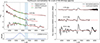 |
Fig. 1. Example of the LOWESS-based continuum removal applied to selected spectra of SN 2012aw. Top left: Original spectra with the LOWESS-smoothed continuum overplotted. The yellow marker indicates a reference wavelength at which the local linear fits are displayed for each spectrum. The blue shaded region highlights the masked Hα feature, excluded from the continuum fitting to avoid bias Bottom left: Shape of the LOWESS kernel at the reference wavelength, illustrating the weighting scheme used during smoothing. Right: Continuum-normalized spectra obtained by dividing the original data by the LOWESS continuum fit. |
3.2. Denoising of spectra
After normalizing each spectrum by its continuum, we performed a denoising step to minimize the influence of noise on subsequent analyses. Although Principal component analysis (PCA, Pearson 1901) is generally effective at isolating random noise, we opted to denoise beforehand due to specific characteristics of our sample: many spectra, particularly at earlier phases, exhibit higher noise levels in the red end due to relatively lower fluxes, and spectroscopic fringing signatures are also present in several cases (e.g., the spectrum of SN 2012aw at 5.35 days shown in right panel of Fig. 1). These nonrandom patterns can contaminate the principal components if not addressed in advance.
To mitigate this contamination, we fit the normalized spectra with a combination of Gaussian processes1 (GP; Rasmussen & Williams 2006), using the GEORGE Python package. To capture the variability of the spectra, we split each spectrum at 7000 Å into a blue and a red region, allowing for different GP kernel configurations tailored to the noise properties on each side. This division was motivated by the fact that fringing affects broader wavelength scales, particularly in the red, while random noise affects the blue region more at later phases, which contains finer spectral features (e.g., line blanketing features), and that would be lost with overly broad smoothing. For each segment, we modeled the data using two additive GP components, one for the signal and one for the noise:
-
Noise model: For the noise, a product of a sinusoidal kernel (to capture oscillatory noise) and an exponential kernel (to model variations in noise amplitude, e.g., those introduced by the continuum normalization).
-
Signal model: Two Matern-32 kernels with two different length scales: one short (to capture features such as emission and absorption lines), and a long one (to follow smoother variations such as residual continuum structure).
The specific kernel parameters used for the denoising are listed in Table 1. Each spectrum was fit on the blue and red sides using the sum of the corresponding GP kernel combinations, effectively separating noise from the underlying spectral features. Fig. 2 shows a representative outcome of the denoising process. To verify that only noise was removed, we examined the distribution of the extracted noise term. Assuming white noise, this distribution should follow a Gaussian profile; any significant deviation would suggest that parts of the actual spectrum were accidentally modeled as noise. As shown in the figure, the noise component closely matches a Gaussian distribution, indicating that the denoising procedure effectively suppresses noise without significant losses in the spectrum. This denoising step was applied to all continuum-normalized spectra. All subsequent analyses were carried out on the denoised data. For reference, we also performed the full analysis on the original (nondenoised) dataset, and the test results are presented in Appendix A.
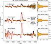 |
Fig. 2. Gaussian process denoising applied to example spectra of SN 2015bs. The left plot shows the original spectra overlaid with their denoised counterparts, demonstrating the effectiveness of the procedure in preserving spectral features. The right panel shows histograms of the flux residuals attributed to noise. The near-Gaussian distribution of these residuals supports the assumptions of white noise and confirms that no significant correlated features were removed during the process. |
Parameters used for Gaussian process denoising.
4. Analysis
4.1. Standardizing the spectra to given epochs
This study investigates spectral diversity and continuity across the SN IIP/L subtypes. Previous analyses of SNe II have suggested that these events form a continuous class, with no clear dichotomy in either their light curve or spectral properties (see e.g., Anderson et al. 2014b,a; Gutiérrez et al. 2014, 2017a,b). While spectroscopic differences have been observed, these variations appear continuous rather than two separate subclasses. For instance, Gutiérrez et al. (2014, 2017a) showed a correlation between the shape of the Hα P-Cygni profile and the light curve decline rates, with more rapidly declining SNe II showing suppressed Hα absorptions. This trend is also evident in our sample.
One challenge in identifying robust spectral trends related to the light curve decline rates lies in the variation of observational epochs across different SNe. To mitigate this, previous works such as Anderson et al. (2014a) and Gutiérrez et al. (2017a) focused on single spectral features (e.g., peak blueshifts or Hα absorption-to-emission ratios), which were then interpolated to a common epochs for comparison. In this work, rather than limiting the analysis to a single spectral parameter, we undertake a full spectral time-series comparison. To do this, instead of interpolating a single parameter, we interpolate the entire spectral time evolution across a range of common epochs. Our method follows the GP interpolation approach similar to that outlined in Saunders et al. (2018) and Léget et al. (2020). First, each spectrum was rebinned onto a uniform wavelength grid spanning 3500 and 9500 Å. We then applied GP independently to each wavelength bin in the time series of each SN. As in Saunders et al. (2018), we did not enforce correlations between neighboring wavelength bins, both to reduce computational cost and because including such correlations did not significantly improve interpolation accuracy, particularly given the intrinsic spectral diversity of SNe II. Fig. 3 illustrates the GP-based spectral interpolation process. Using this method, we reconstructed complete spectral sequences across the early photospheric phase and interpolated spectra for each SN at four common epochs: 20, 30, 40 and 50 days post-explosion. These interpolated spectra are then used for the subsequent comparative analyses.
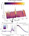 |
Fig. 3. Illustration of the Gaussian process-based interpolation of the spectral time series. Panel (a) 3D view of the continuum-normalized spectral time series of SN 2007od interpolated onto a common time–wavelength grid. Panel (b) projection of panel (a), collapsed along the time axis, highlighting the evolution of spectral changes in the region around Hα. Panel (c) flux evolution at a given wavelength bin (red dashed line in panels (a) and (b)), with GP fit color-coded by epoch. |
4.2. Dimension reduction via PCA
To reduce the dimensionality of the spectral dataset and facilitate the comparison between objects, we applied PCA to the spectra at each selected epoch independently. PCA is widely used in astronomy for dimensionality reduction and identifying the directions of greatest variability within a dataset (see e.g., Hsiao et al. 2007; Müller-Bravo et al. 2022; Burrow et al. 2024; Aamer et al. 2025; Müller-Bravo et al. 2025). Although PCA can be suboptimal for spectra where key features shift significantly in wavelength (such as SN features, where the photospheric velocity introduces a range of Doppler shifts), we used it here due to its ease of implementation and interpretability. Fig. 4 shows the results of the PCA applied to the sample spectra at 20 days post-explosion (Figure C.1 shows the 40-day epoch case). At all epochs considered (20, 30, 40 and 50 days post-explosion), the derived eigenspectra reveal that spectral variability spans multiple wavelength regions: none of the most significant components isolate changes in a single feature alone. This implies strong correlations between spectral features at each epoch, suggesting a coherent evolution across the spectrum.
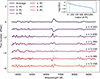 |
Fig. 4. PCA results at one representative epoch. The figure shows the PCA applied to continuum-normalized spectra at 20 days post-explosion. The top spectrum represents the mean SN II spectrum at that epoch, while the spectra below show the first few eigenspectra derived from the PCS (via singular value decomposition, SVD), ordered from top to bottom by decreasing significance. For reference, the mean spectrum is overplotted in light gray behind each eigenspectrum. The numbers next to each eigenspectrum indicate the corresponding eigenvalue, which reflects the variance explained by that PC. The inset plot in each panel displays the eigenvalue decay, indicating the variance captured by each component. |
Another noteworthy trend is observed in the distribution of the singular values (Table C.1), representing the proportion of variance explained by each principal component. Although direct comparison of singular values across PCA runs is limited (due to differences in the number of input spectra at earlier epochs), we observe a general increase in total variance toward later epochs. This is consistent with the emergence and strengthening of spectral lines over time. Additionally, at later epochs, the variance becomes more concentrated in the first few components, indicating that the spectral diversity decreases with time, and a smaller number of components can capture the bulk of the variance. As we discuss later, one possible explanation for the observed excess variability is the early-time interaction between the ejecta and CSM (Gutiérrez et al. 2017b), after which a “normal” SN II spectrum can emerge (e.g., Hillier & Dessart 2019). Still, differences in the SN initial conditions, such as explosion energy or density profile, might also yield more pronounced differences at earlier phases (Valenti et al. 2016).
From the PCA decomposition, we obtained principal component coefficients for each SNe at each epoch. These coefficients serve as a compressed, low-dimensional representation of the original spectra. For the subsequent analysis, we saved the first 70 coefficients per epoch, which were found to account for ∼99% of the total variance. The remaining higher-order components primarily reflect random noise or negligible features.
4.3. Clustering and groups within SN II space
The PCA decomposition provides a compact, lower-dimensional representation of the spectral diversity in our sample, enabling the identification of potential clustering. Our primary objective is to determine whether slow- and fast-declining SNe exhibit a distinct break in their spectral appearance, resulting in clear dichotomies in the PCA coefficients, or whether they form a continuous distribution in the spectral parameter space. Given the high dimensionality of the PCA coefficients (70 per object per epoch), a two-dimensional projection is necessary for visual interpretation. Several nonlinear dimensionality reduction algorithms exist for this purpose, such as t-distributed stochastic neighbor embedding (t-SNE; Van der Maaten & Hinton 2008). t-SNE an unsupervised algorithm that is highly effective at preserving local relationships between data points. At the same time, it enhances distinctions in high-dimensional space as well. Unlike PCA, t-SNE is a nonlinear method that does not yield easily interpretable parameters or axes; however, it offers a powerful tool for revealing latent structures and clusters.
We implemented t-SNE using the OPENTSNE package (Poličar et al. 2024), which offers improved computational efficiency and the ability to embed new data points into existing t-SNE regions. We applied this technique to the PCA coefficients set at 20, 30, 40, and 50 days post-explosion. The result projections are presented in Fig. 5, using consistent hyperparameter settings across epochs. As shown in the figure, the progression of clustering with time is evident. At day 20, most SNe form a single, diffuse cloud with no well-pronounced outliers. Between days 30 and 40, this cloud begins to fragment, and by day 50 a clearer separation emerges, revealing a subgroup with nonstandard spectra (highlighted by the yellow box in the bottom right panel of Fig. 5), and a continuous group of “spectroscopically normal” (canonical) SNe IIP/L. At days 30 and 40, it is possible to recognize a subgroup of objects with weak (suppressed) spectral features and fast-declining light curves (corresponding to canonical IIL-s, middle of top right panel of Fig. 5) and a small subset of slow-declining, low-luminosity SNe II (right center of top right panel of Fig. 5). By day 50, these two subsets merge into the “continuous” group, indicating that their spectral differences are less pronounced than those characterizing the marked subgroup.
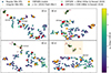 |
Fig. 5. t-SNE projection plots of the PCA coefficients (per epoch). These plots show how the SNe are distributed within the high-dimensional PCA space after dimensional reduction. Colored pentagons mark the positions of different CMFGEN models variants. SNe 2023ixf and 2024ggi are also added using the spectra currently available in the literature (red crosses), along with CSM-interacting SNe II from Jacobson-Galán et al. (2024) (green stars). A clear separation by s2 values is observed across all epochs, confirming the link between spectral and light curve properties. At 50 days, two groups emerge: a continuous “regular SNe IIP/L” sequence along s2, and a scattered subgroup, likely shaped by strong CSM interaction (marked by the yellow rectangle). Model projections align with expectations: CSM-rich models explain the subgroup objects, while mass-loss models resemble fast-declining SNe. |
We tested whether the emergence of this subgroup could be attributed to random alignment or to a robust feature of our sample by applying both trimming and bootstrapping. In the trimming approach, we randomly removed 5% (10%) of the objects from the sample before applying t-SNE. For the bootstrapping test, we have drawn 63% of the full dataset, allowing for duplicates. Clusters were identified using Gaussian mixture models (GMM) from the sklearn package. We recovered comparable groups containing at least 50% of the original subgroup members and less than 25% contamination in 92% (74%) of the trimming realizations. A subgroup matching the conditions also emerges in ∼60% of the bootstrapping cases. These resampling tests indicated that the identified subgroup is not driven by a small number of individual objects, but instead shows moderate stability under perturbations of the dataset. This is consistent with a weakly separated low-count structure in the present sample. We emphasize, however, that the bootstrap recovery fraction derived above should be interpreted as a measure of robustness under resampling, rather than as a formal assessment of statistical significance2. We explore the interpretations of this subgroup in more detail in Sect. 5.
To expand the comparison through t-SNE, we included observational data of SN 2023ixf and SN 2024ggi, as well as CMFGEN SN II models (Dessart et al. 2013, 2017; Lisakov et al. 2017; Hillier & Dessart 2019), along with CSM interacting SNe II from Jacobson-Galán et al. (2024), which exhibited strong flash features3 To include these events, we estimated their PCA coefficients based on the main sample and then projected them onto our 2D t-SNE embedding using OPENTSNE. For SN 2023ixf, we used data from Zheng et al. (2025), while the SN 2024ggi data were obtained from Ertini et al. (2025). Due to the lack of spectroscopic coverage between 30 and 50 days for SN 2024ggi, it is only included in the 20- and 30-day projections.
Both SN 2023ixf and SN 2024ggi are located at the interface between the main population (regular SNe) and the detached subgroup. This placement is consistent with signatures of early CSM interaction, which delays and suppresses the appearance of P-Cygni profiles. Given the strong suppression or lack of P-Cygni features at early stages, both objects are mixed with canonical IIL-s in Fig. 5. In the case of SN 2023ixf, the emergence of more typical features after day 30 results in its migration toward the main group, though the absorption and emission features remain weaker than average. A similar transition is expected for SN 2024ggi, although this cannot be directly confirmed due to the missing epoch coverage.
The positions of the CMFGEN models align well with the various subpopulations of SNe IIP/L and reproduce our expectations of the models. The majority of the models from Dessart et al. (2013, 2017), Lisakov et al. (2017) have projected positions on the t-SNE plots that align well with the more canonical IIP-type SNe, with only a number of models scattering among SNe IIL that exhibit steeper light curve decline rates. The situation changes with the addition of models from Hillier & Dessart (2019), which include model runs with CSM interaction through density profile modifications and mass loss. The models that assume mass loss of the progenitor before the explosions (with model names as “x*p0” in Hillier & Dessart 2019) are placed among the SNe that exhibit relatively high decline rates of s2 ∼ 3 mag / 100d. Interestingly, these models are the most similar to one another, which could imply that the variations caused by mass loss and reduced hydrogen envelope cannot account for all the diversity observed in the IIL subclass (at least within the modeling framework established in Hillier & Dessart 2019).
Furthermore, these models exhibit notable differences in spectral appearance compared to SNe 2023ixf and 2024ggi. In contrast, models assuming CSM interaction can produce spectra that closely resemble those of these two SNe. Fig. 6 shows the comparison of the spectra of SNe 2023ixf and 2024ggi at 20 and 30 day epochs with the models from Hillier & Dessart (2019) that fall the closest to them on the t-SNe plots corresponding to these epochs. The first best match is given by x3p0ext5, with x3p0ext4 also yielding an adequate comparison to SN 2024ggi at 20 days. These models assume an intermediate amount of CSM interaction in the model grid. Given that the early-time behavior of the above two SNe is explained as being influenced by CSM interaction, the recovered match with the models that assume a similar behavior demonstrates the reliability of our projecting and clustering method.
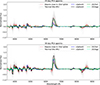 |
Fig. 6. Comparison between the day 20 and day 30 interpolated spectral features of 2023ixf and 2024ggi with the nearest models from Hillier & Dessart (2019), based on Fig. 5. |
Finally, the CSM interacting objects from Jacobson-Galán et al. (2024) are found to cluster almost exclusively within the detached subgroup, together with a single CMFGEN model (x3p0ext6), which assumes the highest scale of interaction with CSM. This overlap strongly supports the interpretation that the subgroup consists of SNe that experienced enhanced CSM interaction. Although the spectra within this group display considerable diversity, a common characteristic is the significant delay in the emergence of P-Cygni features in the spectra, which is usually attributed to CSM interaction. Furthermore, this comparison shows well that SNe exhibiting prevalent and strong flash features, hence having gone through enhanced early CSM interaction, appear significantly different even at later phases, well after the CSM has been swept up by the ejecta.
4.4. Measurement of reference parameters
To compare the spectral properties to a number of easily measurable physical parameters, we estimated the light curve decline rate in the photospheric phase (s2), the Hα absorption-to-emission ratio (a/e), and the Hα absorption line velocity (vHα). For the s2 parameter, we adopted published V-band decline rates wherever available, most notably from Anderson et al. (2014b) for the CSP-I sample. These values and their sources are listed in Table D.1. For SNe lacking literature values, we measured s2 directly following the methodology outlined in Anderson et al. (2014b), ensuring consistency across the dataset. Fig. E.1 in the Appendix shows the sample light curves, with the subgroups defined in Sect. 4.3 highlighted for comparison. For the spectroscopic parameters, we developed an automated and uniform fitting method applied to all sample spectra. To measure line velocities, we first estimated the local continuum slope around the Hα absorption feature, using the continuum fitting approach described in Section 3.1. This slope served as the basis for estimating measurement uncertainties: we generated 100 realizations of each spectrum by applying small random tilts, reflecting the continuum variability. For each realization, we fit the Hα absorption profile using a Generalized additive model (GAM)-based approach (Hastie & Tibshirani 1986), which effectively followed the change in the line profile. GAMs, constructed from linear combinations of spline functions, are nonparametric and flexible. They are well-suited to asymmetric or irregular line profiles without requiring specific profile assumptions (e.g., Gaussian or Lorentzian). The fits were performed over the absorption component of the Hα P-Cygni profile, between 6250 Å and the maximum of the line, which was set iteratively. We defined the absorption line velocity as the wavelength corresponding to the minimum of the fit profile. While this measurement could have been conducted on the continuum-normalized spectra, we retained the original continuum to ensure consistency with the methodology of Gutiérrez et al. (2017b).
To determine Hα (a/e), we first estimated the local continuum across the line profile by fitting a linear baseline to the edges of the feature, identified using the continuum-normalized spectra. We opted not to measure the a/e directly from the normalized spectra, as the continuum is often curved underneath the line, which could potentially introduce bias. Once the continuum was defined, we integrated the absorption and emission components to compute their pseudo-equivalent widths (pEWs) using the simps integration method from SCIPY package (Virtanen et al. 2020).
Fig. 7 shows a corner plot comparing the derived parameters for our SN sample. For the CSP-I sample, we also display literature values from Gutiérrez et al. (2014) and Gutiérrez et al. (2017b) for validation. Overall, we find good agreement between our measurements and those from the literature. A small systematic offset of ∼10% in the Hα emission strength relative to Gutiérrez et al. (2017b) is observed, likely due to differences in the continuum placement during the pEW estimation. Our reanalysis further confirms known correlations among the parameters, most notably between s2 and a/e, reinforcing the link between light curve decline rates and spectroscopic evolution. Importantly, these observables show a clear continuity rather than a dichotomy, supporting that SNe IIP and IIL represent opposite edges of the same continuous SN class. This remeasurement is both a partial confirmation and an important sanity check for the results of our data-driven approach.
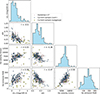 |
Fig. 7. Cornerplot of the measured spectral and light curve parameters for our supernova sample (blue and yellow squares together) at the epoch of 50 days. The blue circles represent the supernovae that belong to the “continuous” subclass of SNe II, while the yellow squares are the objects that are members of the detached subgroup based on their spectral appearance and the clustering performed in Sect. 4.3. The red circles represent the measurements done in Gutiérrez et al. (2017b), for comparison. The τ values are the Kendall-tau correlation parameters for the canonical SNe. |
4.5. Spectral differences for IIP/L: Gradual change of features across light curve decline rates
A long-standing question in the study of SNe II is how spectral features correlate with the light curve decline rate. Previous empirical studies have largely focused on the most prominent optical emission line, Hα, finding that for fast-declining (IIL) SNe, the Hα line is increasingly blueshifted and its absorption profile weakens (Anderson et al. 2014a; Gutiérrez et al. 2014, 2017a). We independently confirm these effects and uncover further correlations across the full optical spectral range.
By normalizing and interpolating the spectra, we were able to systematically and simultaneously examine how spectral features vary with the light curve s2 across the entire wavelength range. This was done by computing a moving median of each PCA coefficient as a function of s2 (ranging from 0 to 2.5 [mag/100 d]), using a window width of 1 [mag/100 d]. The median spectra were then reconstructed by linearly combining the corresponding PCs. Since the individual principal components are linearly independent (by definition of PCA), this reconstruction could be performed by taking the sum. Objects that formed a detached subgroup in Fig. 5 were excluded from this analysis.
Although this method cannot capture the full spectral diversity, only mean trends, it reveals a clear connection between s2 and the spectra. As shown in Fig. 8, significant correlations exist even among spectroscopically “normal” SNe II. The strength and nature of these correlations evolve with time: at early epochs (e.g., day 20), Hα shows a strong dependence on s2, while at later epochs (e.g., at day 50), differences become more subtle. Besides Hα, the Ca II near-infrared (NIR) triplet also varies with the decline rate, and correlated changes are also observed across the metal line blanketing region. Notably, the strengths of Hγ and the Fe II lines seem to correlate with s2, while Hβ appears largely unaffected.
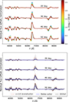 |
Fig. 8. Top: Median reconstructed spectral trends as a function of the s2 light curve decline rate based on our PCA analysis. The four sets of spectra correspond to the four investigated epochs. The color of the individual spectra shows the s2 light curve decline rate for which they were calculated. Bottom: Subgroup spectra. The gray spectra show those of the subgroup objects (defined by Fig. 5, the blue spectra show their median for each epoch. The red dashed spectrum shows the reconstructed spectrum for s = 2.5 [mag/100 d] (which is the darkest red spectrum on the left-hand side plot), while the black curve shows the spectra of SN 2023ixf. |
We note that establishing the connection between PCs and external parameters such as s2 is inherently flexible and can be approached in multiple ways. While PCA facilitates dimensionality reduction, outlier identification, and reconstruction, the trends present between the spectral appearance and the decline rate can be qualitatively shown without applying it. This is shown in Appendix B, in Fig. B.1, where we plot the sample spectra between epochs 25 and 35 days for decline rates below and over s2 = 1.5 [mag/100 d], both before and after the continuum normalization. The simple check aligns well with the trends recovered by the PCA analysis; larger decline rates lead to more suppressed spectral features.
We further tested the robustness of the trends shown in Fig. 8 by evaluating their dependence on the chosen median filter or regression method. In addition to the moving median approach, we explored two alternative techniques: fitting a linear function to the PC – s2 relationship, and applying a random forest regressor. While the exact scaling of the spectral features is slightly different in each setup, all approaches yielded qualitatively consistent results: spectral features (especially Hα and the Ca II NIR triplet) are suppressed and blueshifted with higher s2 values, alongside correlated changes in the metal line blanketing region.
To contrast this with the detached subgroup, the right panel of Fig. 8 presents their denoised and interpolated spectra. The dominant difference is the overall suppression of spectral features in the subgroup objects compared to the continuous set. This is consistent with early-time CSM interaction, with ejecta not optically thick enough to form narrow lines.
5. Discussion
In the above sections, we demonstrated how spectral interpolation across epochs, combined with dimensionality reduction techniques, can be effectively used to uncover correlations between SN-specific parameters and spectral shapes. We employ principal component analysis as a basis for our work, similarly to other data-driven studies into SN spectra, such as Lu et al. (2023) or Burrow et al. (2024).
At the core of the method is the continuum normalization step, which significantly mitigates the impact of flux calibration uncertainties and unknown reddening. The approach successfully reproduces well-established correlations reported in earlier studies (e.g., Gutiérrez et al. 2014 and Gutiérrez et al. 2017a), while offering the added benefit of enabling comparison between spectra at fixed epochs across the entire optical range, rather than being limited to a small set of specific descriptive parameters.
As discussed in Sections 4.3 and 4.5, the spectra of SN IIP/L reveal both a degree of continuity and a certain level of dichotomy. Fig. 5 highlights a meaningful separation: one subset of SNe displays well-defined correlations (especially in the appearance of Hα), while another group deviates from this trend, showing unusual or strongly suppressed line profiles. We note that this distinction is not clear-cut in earlier phases: the separation becomes apparent only at later phases (day 50) in our analysis. At earlier phases, the data exhibit larger variability, which smears the dichotomy observed at later phases. Many of these subgroup objects are explained through CSM interaction, such as for objects from Pessi et al. (2023), which supernovae generally also exhibit steeper light curve declines and suppressed spectral features. In addition to these cases, a few SNe display atypical behavior, for instance, SNe 2016bkv (Hosseinzadeh et al. 2017) or 2018zd (Hiramatsu et al. 2021b) show narrow P-Cygni lines, while SN 2020cxd (Yang et al. 2021) is notable for its peculiar late-time rebrightening during the end of the plateau phase. Projecting SNe exhibiting strong flash features from the Jacobson-Galán et al. (2024) sample also supports the interpretation of enhanced CSM interaction, as these events show remarkable overlap with the subgroup found in the t-SNE space.
This is also supported by the comparison with the radiative transfer models from Hillier & Dessart (2019). While the models assuming steady mass loss, which reduces the hydrogen envelope mass, are similar to SNe exhibiting steeper light curve declines, they cannot explain the full spectral variability in the sample. The models assuming CSM interaction encompass a larger range in spectral diversity, and similarities can be found with members of the subgroup, the transitional objects similar to 2023ixf, and the more canonical IIP-s as well. At later phases, however, the CSM interacting models show slightly differing spectra from canonical IIL-s, which may indicate that a more complete (and likely, more computationally expensive) treatment of mass loss and CSM interaction would be necessary in the models to fully explain the spectral diversity.
Our resampling analysis suggests that the emergence of a subgroup is not an artifact of the t-SNE representation, and it shows moderate stability in our sample. However, we suspect the separation of the subgroup only reflects the low number of such objects in our sample. In Fig. 5 we showed that the subgroup is connected to enhanced CSM interaction, which should scale continuously, hence the subgroup is likely only one extreme of the underlying continuum.
Observing additional objects with similar or stronger CSM interacting signals than 2023ixf or 2024ggi will likely reveal a continuity toward these objects too. It is important to note, however, subgroup objects identified in the embedding remain distinct in the direct correlations of spectroscopic observables, particularly those involving the strength of Hα (Fig. 7). This supports the interpretation that enhanced CSM interaction significantly alters the Balmer line profiles, weakening the empirical correlations followed by canonical SNe II. This conclusion is consistent with the recent findings of Dessart & Jacobson-Galan (2026), who also demonstrated that the Hα profile serves as a key tracer of CSM interaction at earlier phases.
Within the canonical subset of SNe, we recover continuous changes in the spectral appearance between SNe IIP and IIL, as shown in Sect. 4.3 and Sect. 4.5. This manifests as subtle but systematic trends across the s2 decline rates, which are more pronounced at earlier phases, in line with the higher spectral diversity at these times found through PCA. A plausible explanation for this early-time diversity is CSM interaction, which can suppress and delay line profiles, as also noted by Hillier & Dessart (2019), thereby introducing greater variation and partially masking the intrinsic similarities among explosions. These differences likely become more subtle once the CSM is swept up by the SN ejecta and ceases being a dominant source of extra light. However, other physical factors may also contribute to the observed early phase diversity, including variations in explosion energy, envelope density profile and radius, Ni-mixing, nonlinear temperature effects, all of which can affect the line profiles in the first weeks when the photosphere is probing the outer, still hot regions of the ejecta. On the other hand, at later phases, when the hydrogen recombination dominates, these effects are expected to even out, reducing the overall spectral diversity (Dessart & Hillier 2011; Valenti et al. 2016).
As shown by the reconstructed spectra for the continuous sample (Fig. 8), the variation along s2 manifests primarily as a progressive suppression of spectral features across the entire wavelength range at earlier phases. This effect is particularly pronounced at the 30-day epoch, where fast-declining SNe (IIL) display weaker Hα absorption and emission, reduced Ca II NIR triplet strength, and diminished metal line blanketing. These consistent patterns further support the interpretation that s2 encodes meaningful information about the physical conditions of the explosion (e.g., hydrogen envelope mass) and the degree of interaction with the circumstellar medium (CSM). The findings align well with those indicating that the class of SNe II, especially SNe IIP/L, forms a continuity, rather than a set of distinct subgroups. This was first suggested based on light curve (Anderson et al. 2014b) and spectral properties (e.g., Anderson et al. 2014a; Gutiérrez et al. 2017a), and further supported by radiative transfer models (Hillier & Dessart 2019). More recent studies using early light curves and rise times (e.g., Nagao et al. 2020; Hinds et al. 2025; Ertini et al. 2026) have strengthened this unified scenario.
Although our spectral reconstructions focus on SNe with s2 = 2.5 mag/100 day, the steeper-declining events from Pessi et al. (2023) show spectral trends observed that are consistent with the broader patterns observed. While we did not include these objects for reconstructing the average trends shown in Fig. 8 due to a small sample size, they are included in the qualitative check in Appendix B. These objects tend to represent intermediate cases between standard SNe II and SNe IIn, likely shaped by enhanced CSM interaction. Their alignment with the overall trends suggests that the varying degree of CSM interaction plays a key role in driving the observed changes in spectral features, particularly at the high end of the s2 distribution.
Understanding the continuity and spectral diversity of SNe II is crucial for their use as standard candles (Poznanski et al. 2009; de Jaeger et al. 2022). The observed correlations between spectroscopic and photometric parameters are promising for calibrating absolute magnitudes. However, the presence of a spectral subgroup in our quality-selected sample cautions against treating all SNe IIP/L as a homogeneous population for standardization. While we suspect the current gap is due to the low SN count will be bridged by future observations and more complete sample, the presence of a subgroup of objects showing enhanced CSM interaction and following trends different from the canonical sample (with all the subset objects being outliers for the correlations in Fig. 7) highlight the need for additional standardization parameters that can account for their diversity. This issue is especially relevant for applying the method to events such as SN 2023ixf (see Zheng et al. 2025). Although it benefits from accurate calibrator distances (e.g., Huang et al. 2024), SN 2023ixf lies on the interface of the spectroscopic subgroup, where correlations are altered.
A natural extension of the method is its potential use as a classification tool for new SNe. On the one hand, the simplest approach is to incorporate some of the interpolated spectra as templates to the currently existing classifiers, such as SNID (Supernova Identification, Blondin & Tonry 2007) or GELATO (Harutyunyan et al. 2008). This would extend these classifiers to better cover the more “irregular” or “CSM-interacting” members of the SN II population, which are currently underrepresented in standard template libraries. However, these template matching methods only perform the comparisons at a single, discrete epoch. This made sense in the past, given the limited sampling of observations. A more powerful approach would involve comparing the full time evolution of a supernova’s spectrum against a library of interpolated spectral series. Instead of matching a single spectrum, this method would identify the object whose spectral evolution most closely mirrors that of the target, effectively finding its “spectroscopic twin”. Our interpolation technique is ideally suited for such comparisons, allowing consistent spectral matching across all available epochs.
The idea of using spectral interpolation for classification purposes has recently been explored by other works as well: for instance, Ramirez et al. (2024) used spectral interpolation to improve photometric classification of SNe. As they cite, their method can further be used to estimate the necessary K-correction to be applied to photometry. Likewise, Vincenzi et al. (2019) demonstrated how spectrophotometric templates can be created purely on an observational basis, by interpolating high-quality spectral time series with photometry. While being the most complete approach, their method requires high-quality observations and an assumption on the total reddening toward the SN, which poses a limitation. In contrast, our approach can complement the above by not only identifying the type but also proposing a set of objects that evolve spectroscopically similar to previously observed batches, while being less susceptible to observational effects, similar to SNID. It also offers the possibility of estimating the explosion time from spectroscopy alone, an important capability when early photometry is missing. We plan to explore these directions further in a future work.
It is important to note that the found correlations are limited by the precision in estimating the explosion time (t0) for individual SNe. While this introduces statistical uncertainty, which we did not propagate into the analysis at this stage. Limiting ourselves to objects with better-defined t0 reduces our exposure to this issue. Furthermore, for most of our sample, particularly spectra from the past decade, t0 is known to within a few days thanks to extensive all-sky survey coverage.
Future works extending on the basis presented here will not be exposed to this problem, owing to the multitude of already working automated wide-field surveys, such as the Zwicky Transient Facility (ZTF, Bellm et al. 2019; Graham et al. 2019), or the Asteroid Terrestrial impact Last Alert System (ATLAS, Smith et al. 2020), the Gravitational-wave Optical Transient Observer (GOTO, Dyer et al. 2020) or the BlackGEM survey (Bloemen et al. 2016), along with the long awaited Vera Rubin LSST survey (Ivezić et al. 2019). Combining these wide-field survey data of the transients with the rapid spectroscopic follow-up triggered by the community will yield a wealth of data where the time of explosion can be pinned down to high precision.
6. Summary and conclusions
In this paper, we utilized time-series interpolation and dimensionality reduction techniques, such as Gaussian process-based time series reconstruction and principal component analysis to uncover correlations between spectral features and light curve decline rates. Our primary goal was to investigate potential spectral differences between SNe IIP/L, that do not exhibit long-lasting narrow emission features characteristic of SNe IIn. We based our analysis on publicly available SN IIP/L data, either from published surveys or more targeted SN works.
To minimize uncertainties related to flux calibration and reddening, we made use of empirical continuum normalization in our work. We then processed the resulting “feature spectral time series” by interpolating them per wavelength bin onto a fixed time grid. These interpolated spectra were subsequently analyzed with PCA to identify correlations between the spectral features and the light curve decline rates.
The main findings of our analysis can be summarized as follows:
-
Flattening the spectra provides a simple and effective tool for combining observations from different surveys and instruments.
-
Spectral diversity of SNe IIP/L decreases with time: by 40–50 days post-explosion, SN spectra become more homogeneous (they exhibit smaller variability) compared to earlier epochs. CSM interaction is expected to be stronger at early phases and may play a major role in driving this effect; however, variations in the initial conditions of the explosion, such as its density profile, Ni-mixing and explosion energy, are also likely to contribute.
-
Most SNe II in our sample form a continuous spectroscopic group across all features, along with a subgroup likely explained by enhanced CSM interaction. This interaction is strong enough to affect early spectra, but the CSM is not optically thick enough to produce long-lived narrow emission lines, as confirmed through a comparison to CSM interacting objects from Jacobson-Galán et al. (2024). This subgroup showed moderate stability (∼60% bootstrap recovery) under our resampling tests, and could be identified in a data-driven way. These objects do not follow the standard empirical correlations between spectroscopic properties, indicating that CSM interaction can significantly affect line profiles. The subgroup members likely represent the extremes of the spectroscopic distribution within the present sample, where pronounced CSM interaction-induced changes in the spectra, combined with their relatively small numbers, lead to their apparent separation from the bulk of SNe II. Future observations of SNe II exhibiting intermediate levels of CSM interaction will be essential for mapping the transitions required to populate the region between the subgroup and the bulk of the sample.
-
We observe robust correlations for the rest of the sample between spectral features and the light curve decline rate s2, a proxy for distinguishing Type IIP or IIL SNe. We find that the strength of most spectral features scales with this parameter. We recover past results, such as faster-declining SNe systematically exhibiting diminished emission and sometimes even lacking absorption lines. This trend is visible not only in Hα, but also in the Ca II NIR triplet and the metal line blanketing region. Additionally, we also recover the known blueshifts in line profiles across the spectrum.
-
Spectral comparisons with nearby events (SN 2023ixf and SN 2024ggi) and radiative transfer models from Dessart et al. (2013, 2017), Hillier & Dessart (2019) agree with the trends observed in our sample. The comparison with radiative transfer models suggests that both mass loss and CSM interaction are necessary to explain the full range of spectral diversity.
-
Our analysis can be further extended toward a classification method, making use of the full spectral time series at once. This allows not only the identification of SN types, but also the discovery of spectroscopic “twins” from existing samples and a refined estimate of the explosion epoch based on spectral evolution.
In the future, the method will be further refined and extended for other types of SNe, improving classification tools, and exploring spectral correlations in greater depth. These developments will be valuable for upcoming surveys, such as the Roman Space Telescope Core Community Survey, LSST follow-up efforts, and other transient discovery programs. Finally, tailoring this analysis for SNe II will allow us to further standardize these objects as standardizable candles or to find objects with little or limited CSM interaction that can be modeled reliably for use as cosmological probes.
Data availability
The data, the intermediate results, the interpolated spectral time series, and the code used for the analysis are openly available on the GitHub page of the author https://github.com/csogeza/IIP-L-diversity. This research has made use of the PYTHON packages: NUMPY (Harris et al. 2020), MATPLOTLIB (Hunter 2007), SCIPY (Virtanen et al. 2020), GEORGE (Ambikasaran et al. 2015), ASTROPY (Astropy Collaboration 2022) and PANDAS (pandas development team 2020).
Acknowledgments
The authors would like to thank the anonymous referee for the comments that helped improve the manuscript. GCS acknowledges the generous computational and financial support provided by the European Southern Observatory and the Max Planck Institute for Astrophysics. GCS thanks and appreciates the enlightening and extremely helpful discussions about this project with Christian Vogl, Stefan Taubenberger, and Bálint Seli. CPG acknowledges financial support from the Secretary of Universities and Research (Government of Catalonia) and by the Horizon 2020 Research and Innovation Programme of the European Union under the Marie Skłodowska-Curie and the Beatriu de Pinós 2021 BP 00168 programme, from the Spanish Ministerio de Ciencia e Innovación (MCIN) and the Agencia Estatal de Investigación (AEI) 10.13039/501100011033 under the PID2023-151307NB-I00 SNNEXT project, from Centro Superior de Investigaciones Científicas (CSIC) under the PIE project 20215AT016 and the program Unidad de Excelencia María de Maeztu CEX2020-001058-M, and from the Departament de Recerca i Universitats de la Generalitat de Catalunya through the 2021-SGR-01270 grant.
References
- Aamer, A., Nicholl, M., Gomez, S., et al. 2025, MNRAS, 541, 2674 [Google Scholar]
- Ambikasaran, S., Foreman-Mackey, D., Greengard, L., Hogg, D. W., & O’Neil, M. 2015, IEEE Trans. Pattern Anal. Mach. Intell., 38, 252 [Google Scholar]
- Anderson, J. P., Dessart, L., Gutierrez, C. P., et al. 2014a, MNRAS, 441, 671 [NASA ADS] [CrossRef] [Google Scholar]
- Anderson, J. P., González-Gaitán, S., Hamuy, M., et al. 2014b, ApJ, 786, 67 [Google Scholar]
- Anderson, J. P., Dessart, L., Gutiérrez, C. P., et al. 2018, Nat. Astron., 2, 574 [NASA ADS] [CrossRef] [Google Scholar]
- Andrews, J. E., Sand, D. J., Valenti, S., et al. 2019, ApJ, 885, 43 [Google Scholar]
- Arcavi, I., Gal-Yam, A., Cenko, S. B., et al. 2012, ApJ, 756, L30 [NASA ADS] [CrossRef] [Google Scholar]
- Astropy Collaboration (Price-Whelan, A. M., et al.) 2022, ApJ, 935, 167 [NASA ADS] [CrossRef] [Google Scholar]
- Barbon, R., Ciatti, F., & Rosino, L. 1979, A&A, 72, 287 [Google Scholar]
- Bellm, E. C., Kulkarni, S. R., Graham, M. J., et al. 2019, PASP, 131, 018002 [Google Scholar]
- Benetti, S., Chugai, N. N., Utrobin, V. P., et al. 2016, MNRAS, 456, 3296 [NASA ADS] [CrossRef] [Google Scholar]
- Ben-Hur, A., Elisseeff, A., & Guyon, I. 2002, Pacific Symp. Biocomput., 2002, 6 [Google Scholar]
- Bloemen, S., Groot, P., Woudt, P., et al. 2016, SPIE Conf. Ser., 9906, 990664 [NASA ADS] [Google Scholar]
- Blondin, S., & Tonry, J. L. 2007, ApJ, 666, 1024 [NASA ADS] [CrossRef] [Google Scholar]
- Bose, S., Sutaria, F., Kumar, B., et al. 2015a, ApJ, 806, 160 [Google Scholar]
- Bose, S., Valenti, S., Misra, K., et al. 2015b, MNRAS, 450, 2373 [Google Scholar]
- Bostroem, K. A., Valenti, S., Horesh, A., et al. 2019, MNRAS, 485, 5120 [Google Scholar]
- Bouchet, P., Moneti, A., Slezak, E., Le Bertre, T., & Manfroid, J. 1989, A&AS, 80, 379 [NASA ADS] [Google Scholar]
- Bronner, V. A., Laplace, E., Schneider, F. R. N., & Podsiadlowski, P. 2025, A&A, 703, A61 [NASA ADS] [CrossRef] [EDP Sciences] [Google Scholar]
- Bruch, R. J., Gal-Yam, A., Schulze, S., et al. 2021, ApJ, 912, 46 [NASA ADS] [CrossRef] [Google Scholar]
- Bruch, R. J., Gal-Yam, A., Yaron, O., et al. 2023, ApJ, 952, 119 [NASA ADS] [CrossRef] [Google Scholar]
- Burrow, A., Baron, E., Burns, C. R., et al. 2024, ApJ, 967, 55 [Google Scholar]
- Csörnyei, G., Vogl, C., Taubenberger, S., et al. 2023, A&A, 672, A129 [NASA ADS] [CrossRef] [EDP Sciences] [Google Scholar]
- Dall’Ora, M., Botticella, M. T., Pumo, M. L., et al. 2014, ApJ, 787, 139 [CrossRef] [Google Scholar]
- Dastidar, R., Misra, K., Singh, M., et al. 2019a, MNRAS, 486, 2850 [Google Scholar]
- Dastidar, R., Misra, K., Valenti, S., et al. 2019b, MNRAS, 490, 1605 [Google Scholar]
- Dastidar, R., Misra, K., Singh, M., et al. 2021, MNRAS, 504, 1009 [Google Scholar]
- de Jaeger, T., Galbany, L., Gutiérrez, C. P., et al. 2018, MNRAS, 478, 3776 [CrossRef] [Google Scholar]
- de Jaeger, T., Galbany, L., Riess, A. G., et al. 2022, MNRAS, 514, 4620 [NASA ADS] [CrossRef] [Google Scholar]
- Dessart, L. 2025, A&A, 694, A132 [NASA ADS] [CrossRef] [EDP Sciences] [Google Scholar]
- Dessart, L. 2026, in Encyclopedia of Astrophysics (First Edition), ed. I. Mandel, (Oxford: Elsevier), 706 [Google Scholar]
- Dessart, L., & Hillier, D. J. 2011, MNRAS, 410, 1739 [NASA ADS] [Google Scholar]
- Dessart, L., & Hillier, D. J. 2022, A&A, 660, L9 [NASA ADS] [CrossRef] [EDP Sciences] [Google Scholar]
- Dessart, L., & Jacobson-Galan, W. V. 2026, A&A, 707, A251 [NASA ADS] [CrossRef] [EDP Sciences] [Google Scholar]
- Dessart, L., Hillier, D. J., Waldman, R., & Livne, E. 2013, MNRAS, 433, 1745 [NASA ADS] [CrossRef] [Google Scholar]
- Dessart, L., Hillier, D. J., & Audit, E. 2017, A&A, 605, A83 [NASA ADS] [CrossRef] [EDP Sciences] [Google Scholar]
- Dessart, L., Gutiérrez, C. P., Ercolino, A., Jin, H., & Langer, N. 2024, A&A, 685, A169 [NASA ADS] [CrossRef] [EDP Sciences] [Google Scholar]
- Dhungana, G., Kehoe, R., Vinko, J., et al. 2016, ApJ, 822, 6 [NASA ADS] [CrossRef] [Google Scholar]
- Dyer, M. J., Steeghs, D., Galloway, D. K., et al. 2020, SPIE Conf. Ser., 11445, 114457G [NASA ADS] [Google Scholar]
- Eldridge, J. J., Xiao, L., Stanway, E. R., Rodrigues, N., & Guo, N. Y. 2018, PASA, 35 [Google Scholar]
- Elmhamdi, A., Danziger, I. J., Chugai, N., et al. 2003, MNRAS, 338, 939 [CrossRef] [Google Scholar]
- Ercolino, A., Jin, H., Langer, N., & Dessart, L. 2025, A&A, 696, A103 [NASA ADS] [CrossRef] [EDP Sciences] [Google Scholar]
- Ertini, K., Regna, T. A., Ferrari, L., et al. 2025, A&A, 699, A60 [NASA ADS] [CrossRef] [EDP Sciences] [Google Scholar]
- Ertini, K., Anderson, J. P., Folatelli, G., et al. 2026, A&A, submitted [arXiv:2602.03638] [Google Scholar]
- Fang, Q., Moriya, T. J., Maeda, K., Dorozsmai, A., & Silva-Farfán, J. 2025, ApJ, 990, 60 [Google Scholar]
- Faran, T., Poznanski, D., Filippenko, A. V., et al. 2014, MNRAS, 445, 554 [NASA ADS] [CrossRef] [Google Scholar]
- Filippenko, A. V., Matheson, T., & Ho, L. C. 1993, ApJ, 415, L103 [NASA ADS] [CrossRef] [Google Scholar]
- Galbany, L., Hamuy, M., Phillips, M. M., et al. 2016, AJ, 151, 33 [NASA ADS] [CrossRef] [Google Scholar]
- Gall, E. E. E., Polshaw, J., Kotak, R., et al. 2015, A&A, 582, A3 [NASA ADS] [CrossRef] [EDP Sciences] [Google Scholar]
- González-Bañuelos, M., Gutiérrez, C. P., Galbany, L., & González-Gaitán, S. 2025, A&A, 702, A128 [NASA ADS] [CrossRef] [EDP Sciences] [Google Scholar]
- Graham, M. J., Kulkarni, S. R., Bellm, E. C., et al. 2019, PASP, 131, 078001 [Google Scholar]
- Gutiérrez, C. P., Anderson, J. P., Hamuy, M., et al. 2014, ApJ, 786, L15 [CrossRef] [Google Scholar]
- Gutiérrez, C. P., Anderson, J. P., Hamuy, M., et al. 2017a, ApJ, 850, 90 [CrossRef] [Google Scholar]
- Gutiérrez, C. P., Anderson, J. P., Hamuy, M., et al. 2017b, ApJ, 850, 89 [CrossRef] [Google Scholar]
- Harris, C. R., Millman, K. J., van der Walt, S. J., et al. 2020, Nature, 585, 357 [NASA ADS] [CrossRef] [Google Scholar]
- Harutyunyan, A. H., Pfahler, P., Pastorello, A., et al. 2008, A&A, 488, 383 [NASA ADS] [CrossRef] [EDP Sciences] [Google Scholar]
- Hastie, T., & Tibshirani, R. 1986, Stat. Sci., 1, 297 [Google Scholar]
- Hennig, C. 2007, Comput. Stat. Data Anal., 52, 258 [CrossRef] [Google Scholar]
- Hicken, M., Friedman, A. S., Blondin, S., et al. 2017, ApJS, 233, 6 [NASA ADS] [CrossRef] [Google Scholar]
- Hillier, D. J., & Dessart, L. 2019, A&A, 631, A8 [NASA ADS] [CrossRef] [EDP Sciences] [Google Scholar]
- Hinds, K. R., Perley, D. A., Sollerman, J., et al. 2025, MNRAS, 541, 135 [Google Scholar]
- Hiramatsu, D., Howell, D. A., Moriya, T. J., et al. 2021a, ApJ, 913, 55 [CrossRef] [Google Scholar]
- Hiramatsu, D., Howell, D. A., Van Dyk, S. D., et al. 2021b, Nat. Astron., 5, 903 [NASA ADS] [CrossRef] [Google Scholar]
- Hosseinzadeh, G., Valenti, S., Arcavi, I., McCully, C., & Howell, D. A. 2017, Am. Astron. Soc. Meeting Abstr., 229, 308.06 [Google Scholar]
- Hosseinzadeh, G., Valenti, S., McCully, C., et al. 2018, ApJ, 861, 63 [NASA ADS] [CrossRef] [Google Scholar]
- Hsiao, E. Y., Conley, A., Howell, D. A., et al. 2007, ApJ, 663, 1187 [Google Scholar]
- Huang, F., Wang, X. F., Hosseinzadeh, G., et al. 2018, MNRAS, 475, 3959 [NASA ADS] [CrossRef] [Google Scholar]
- Huang, C. D., Yuan, W., Riess, A. G., et al. 2024, ApJ, 963, 83 [Google Scholar]
- Hunter, J. D. 2007, Comput. Sci. Eng., 9, 90 [NASA ADS] [CrossRef] [Google Scholar]
- Ivezić, Ž., Kahn, S. M., Tyson, J. A., et al. 2019, ApJ, 873, 111 [Google Scholar]
- Jacobson-Galán, W. V., Dessart, L., Davis, K. W., et al. 2024, ApJ, 970, 189 [CrossRef] [Google Scholar]
- Jacobson-Galán, W. V., Dessart, L., Davis, K. W., et al. 2025, ApJ, 992, 100 [Google Scholar]
- Knop, S., Hauschildt, P. H., Baron, E., & Dreizler, S. 2007, A&A, 469, 1077 [NASA ADS] [CrossRef] [EDP Sciences] [Google Scholar]
- Léget, P. F., Gangler, E., Mondon, F., et al. 2020, A&A, 636, A46 [NASA ADS] [CrossRef] [EDP Sciences] [Google Scholar]
- Leonard, D. C., Filippenko, A. V., Li, W., et al. 2002, AJ, 124, 2490 [NASA ADS] [CrossRef] [Google Scholar]
- Leonard, D. C., Kanbur, S. M., Ngeow, C. C., & Tanvir, N. R. 2003, ApJ, 594, 247 [NASA ADS] [CrossRef] [Google Scholar]
- Li, W., Leaman, J., Chornock, R., et al. 2011, MNRAS, 412, 1441 [NASA ADS] [CrossRef] [Google Scholar]
- Lisakov, S. M., Dessart, L., Hillier, D. J., Waldman, R., & Livne, E. 2017, MNRAS, 466, 34 [Google Scholar]
- Lu, J., Hsiao, E. Y., Phillips, M. M., et al. 2023, ApJ, 948, 27 [NASA ADS] [CrossRef] [Google Scholar]
- Maund, J. R., Fraser, M., Smartt, S. J., et al. 2013, MNRAS, 431, L102 [NASA ADS] [CrossRef] [Google Scholar]
- Minkowski, R. 1941, PASP, 53, 224 [NASA ADS] [CrossRef] [Google Scholar]
- Morozova, V., Piro, A. L., & Valenti, S. 2017, ApJ, 838, 28 [NASA ADS] [CrossRef] [Google Scholar]
- Müller-Bravo, T. E., Gutiérrez, C. P., Sullivan, M., et al. 2020, MNRAS, 497, 361 [Google Scholar]
- Müller-Bravo, T. E., Sullivan, M., Smith, M., et al. 2022, MNRAS, 512, 3266 [CrossRef] [Google Scholar]
- Müller-Bravo, T. E., Galbany, L., Stritzinger, M. D., et al. 2025, A&A, 702, A134 [NASA ADS] [CrossRef] [EDP Sciences] [Google Scholar]
- Nagao, T., Maeda, K., & Ouchi, R. 2020, MNRAS, 497, 5395 [NASA ADS] [CrossRef] [Google Scholar]
- pandas development team 2020, https://doi.org/10.5281/zenodo.3509134 [Google Scholar]
- Pastorello, A., Zampieri, L., Turatto, M., et al. 2004, MNRAS, 347, 74 [Google Scholar]
- Pastorello, A., Sauer, D., Taubenberger, S., et al. 2006, MNRAS, 370, 1752 [NASA ADS] [CrossRef] [Google Scholar]
- Pastorello, A., Valenti, S., Zampieri, L., et al. 2009, MNRAS, 394, 2266 [Google Scholar]
- Pearson, K. F. 1901, Lond. Edinburgh Dublin Philos. Mag. J. Sci., 2, 559 [Google Scholar]
- Pearson, J., Hosseinzadeh, G., Sand, D. J., et al. 2023, ApJ, 945, 107 [NASA ADS] [CrossRef] [Google Scholar]
- Pessi, P. J., Folatelli, G., Anderson, J. P., et al. 2019, MNRAS, 488, 4239 [NASA ADS] [CrossRef] [Google Scholar]
- Pessi, P. J., Anderson, J. P., Folatelli, G., et al. 2023, MNRAS, 523, 5315 [NASA ADS] [CrossRef] [Google Scholar]
- Poličar, P. G., Stražar, M., & Zupan, B. 2024, J. Stat. Software, 109, 1 [Google Scholar]
- Poznanski, D., Butler, N., Filippenko, A. V., et al. 2009, ApJ, 694, 1067 [NASA ADS] [CrossRef] [Google Scholar]
- Ramirez, M., Pignata, G., Förster, F., et al. 2024, A&A, 691, A33 [NASA ADS] [CrossRef] [EDP Sciences] [Google Scholar]
- Rasmussen, C. E., & Williams, C. K. I. 2006, Gaussian Processes for Machine Learning [Google Scholar]
- Reynolds, T. M., Fraser, M., Mattila, S., et al. 2020, MNRAS, 493, 1761 [NASA ADS] [CrossRef] [Google Scholar]
- Sahu, D. K., Anupama, G. C., Srividya, S., & Muneer, S. 2006, MNRAS, 372, 1315 [Google Scholar]
- Sanders, N. E., Soderberg, A. M., Gezari, S., et al. 2015, ApJ, 799, 208 [NASA ADS] [CrossRef] [Google Scholar]
- Saunders, C., Aldering, G., Antilogus, P., et al. 2018, ApJ, 869, 167 [NASA ADS] [CrossRef] [Google Scholar]
- Schlegel, E. M. 1990, MNRAS, 244, 269 [NASA ADS] [Google Scholar]
- Shivvers, I., Modjaz, M., Zheng, W., et al. 2017, PASP, 129, 054201 [NASA ADS] [CrossRef] [Google Scholar]
- Smith, K. W., Smartt, S. J., Young, D. R., et al. 2020, PASP, 132, 085002 [Google Scholar]
- Sollerman, J., Yang, S., Schulze, S., et al. 2021, A&A, 655, A105 [NASA ADS] [CrossRef] [EDP Sciences] [Google Scholar]
- Szalai, T., Vinkó, J., Könyves-Tóth, R., et al. 2019, ApJ, 876, 19 [Google Scholar]
- Taddia, F., Stritzinger, M. D., Sollerman, J., et al. 2012, A&A, 537, A140 [NASA ADS] [CrossRef] [EDP Sciences] [Google Scholar]
- Taddia, F., Sollerman, J., Fremling, C., et al. 2016, A&A, 588, A5 [NASA ADS] [CrossRef] [EDP Sciences] [Google Scholar]
- Takáts, K., Pignata, G., Pumo, M. L., et al. 2015, MNRAS, 450, 3137 [CrossRef] [Google Scholar]
- Takei, Y., Ioka, K., & Shibata, M. 2025, ApJ, 992, 137 [Google Scholar]
- Teja, R. S., Singh, A., Sahu, D. K., et al. 2022, ApJ, 930, 34 [NASA ADS] [CrossRef] [Google Scholar]
- Terreran, G., Jerkstrand, A., Benetti, S., et al. 2016, MNRAS, 462, 137 [Google Scholar]
- Tinyanont, S., Ridden-Harper, R., Foley, R. J., et al. 2022, MNRAS, 512, 2777 [NASA ADS] [CrossRef] [Google Scholar]
- Tomasella, L., Cappellaro, E., Fraser, M., et al. 2013, MNRAS, 434, 1636 [NASA ADS] [CrossRef] [Google Scholar]
- Tomasella, L., Cappellaro, E., Pumo, M. L., et al. 2018, MNRAS, 475, 1937 [NASA ADS] [CrossRef] [Google Scholar]
- Valenti, S., Howell, D. A., Stritzinger, M. D., et al. 2016, MNRAS, 459, 3939 [NASA ADS] [CrossRef] [Google Scholar]
- Valerin, G., Pumo, M. L., Pastorello, A., et al. 2022, MNRAS, 513, 4983 [NASA ADS] [CrossRef] [Google Scholar]
- Van der Maaten, L., & Hinton, G. 2008, J. Mach. Learn. Res., 9, 2579 [Google Scholar]
- Vasylyev, S. S., Filippenko, A. V., Vogl, C., et al. 2022, ApJ, 934, 134 [NASA ADS] [CrossRef] [Google Scholar]
- Vincenzi, M., Sullivan, M., Firth, R. E., et al. 2019, MNRAS, 489, 5802 [NASA ADS] [CrossRef] [Google Scholar]
- Virtanen, P., Gommers, R., Oliphant, T. E., et al. 2020, Nat. Methods, 17, 261 [Google Scholar]
- Von Luxburg, U. 2010, Found. Trends. Mach. Learn., 2, 235 [Google Scholar]
- Xiang, D., Wang, X., Zhang, X., et al. 2023, MNRAS, 520, 2965 [NASA ADS] [CrossRef] [Google Scholar]
- Yang, S., Sollerman, J., Strotjohann, N. L., et al. 2021, A&A, 655, A90 [NASA ADS] [CrossRef] [EDP Sciences] [Google Scholar]
- Yaron, O., Perley, D. A., Gal-Yam, A., et al. 2017, Nat. Phys., 13, 510 [NASA ADS] [CrossRef] [Google Scholar]
- Zhang, J., Wang, X., Mazzali, P. A., et al. 2014, ApJ, 797, 5 [NASA ADS] [CrossRef] [Google Scholar]
- Zhang, J., Wang, X., József, V., et al. 2020, MNRAS, 498, 84 [NASA ADS] [CrossRef] [Google Scholar]
- Zhang, X., Wang, X., Sai, H., et al. 2022, MNRAS, 513, 4556 [NASA ADS] [CrossRef] [Google Scholar]
- Zheng, W., Dessart, L., Filippenko, A. V., et al. 2025, ApJ, 988, 61 [Google Scholar]
Gaussian processes or GP are a nonparametric supervised learning method highly useful for regression applied on irregular data. For more details on the technique, we refer the reader to https://scikit-learn.org/stable/modules/gaussian_process.html.
It has been shown that clustering stability depends strongly on the properties of the data and on the degree of separation between structures. In particular, resampling procedures can reduce the recovery rate even for meaningful clusters, particularly when they are small or only weakly separated from the bulk of the sample (e.g., Ben-Hur et al. 2002; Hennig 2007; Von Luxburg 2010). Hence, the recovery rates of low-population structures may not reach 100% under resampling, as such clusters are disproportionately affected (e.g., Hennig 2007).
We included “gold” and “silver” sample objects, which had a sufficient amount of spectra for our GP spectral interpolation. In the end, the included objects were SNe 2017ahn, 2019ust, 2020abjq, 2020pni, 2021tyw, 2022ffg and 2022pgf.
Appendix A: Analysis on original data without denoising the spectra
To provide a comparison to the PCA analysis presented in Sec. 4, and to show the benefits of the denoising described in Sec. 3.2, we repeat the analysis without applying the GP denoising filter on the input spectra. The outcomes of this setup are shown in Figures. A.1 and A.2.
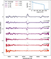 |
Fig. A.1. PCA solution for the 30-day epoch spectra without denoising them in advance. The overall trends and the individual principal components match well those obtained in the run with the applied denoising. The main difference is the lower significance of the PC-s due to the more excessive noise terms that also enter the higher-order components, meaning that more components are necessary for a more reliable decomposition. |
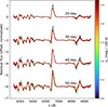 |
Fig. A.2. Recovered spectral features along changes in the light curve decline rate without the use of prior denoising on the spectra. The change in the features along the light curve decline rates matches that presented in Fig. 8: for more significant decline rates, one finds more suppressed emission and absorption lines. |
The principal components displayed in Fig. A.1 resemble those from the denoised case. However, the impact of noise is evident: even the higher-order components display strong noise patterns toward the red end of the spectra. In addition, the significance spectrum changes substantially; it becomes shallower compared to that of Fig. 4, indicating that more PCs are required to explain the same amount of variance. The eigenvalue cutoff also shifts to higher PC indices in the absence of denoising.
Despite these differences, the procedure recovers the same trends between the spectra and the decline rates, as displayed in Fig. A.2. Spectra associated with higher s2 values exhibit more diminished lines, just as shown before. However, the recovered correlations between the change in the spectral profiles and the light curve decline rate are slightly weaker than with denoising. This demonstrates that denoising indeed does not alter intrinsic correlations that can be extracted from the data, but rather strengthens them by removing the correlated effects in the noise (e.g., fringing at the redder wavelengths), leading to a more efficient PCA decomposition.
Finally, we note that our dataset consists of nearby SNe with generally high-quality spectra and overall not so dominant noise components. In contrast, future surveys such as those conducted with the Roman Space Telescope will observe more distant SNe with less optimized follow-up. In those cases, denoising techniques will become even more critical for maximizing the scientific return from lower signal-to-noise spectral data.
Appendix B: Spectral differences between SNe IIP/L without the application of PCA
Ultimately, it is not necessary to apply interpolation or PCA decomposition to qualitatively assess the relationship between spectral features and light curve decline rates. To demonstrate that the recovered trends are not a result of these methods, we divided the SNe into two groups based on their light curve decline rates, using a threshold of 1.5 mag / 100 day to separate the more canonical IIP-s from IIL-s). Fig. B.1 shows the averaged spectra for these two groups at an epoch of 30 +/- 5 days. The comparison reveals that, on average, SNe IIL exhibit more diminished features of hydrogen, along with subtle suppression in the metal line blanketing region and for the Ca II NIR triplet. This low-level test confirms that the spectral differences between SNe IIP and IIL are present directly in the raw data as well, and are not the result of the applied procedure.
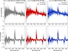 |
Fig. B.1. Spectral differences of IIP and IIL supernovae. The rows correspond to the spectra before and after the continuum normalization. The columns, from left to right: the full sample, the subsample of IIL type supernovae (exhibiting light curve decline rates larger than 1.5 mag / 100 d), and the subsample of IIP supernovae with lower decline rates. The bold colored lines show the medians of the subsamples. |
Appendix C: Principal component analysis results
Details on the principal component analysis applied to the spectra. Table C.1 displays the singular values estimated by PCA, which track the significance of each eigenvector. As an extension of Fig. 4, Fig. C.1 presents the PCA eigenvectors obtained for the spectra at the 40-day epoch.
Singular values estimated by the PCA for individual epochs.
Appendix D: Sample summary
Tables D.1, D.2, and D.3 list the sample objects and the properties used or measured for the analysis. The codes for the references are listed in the caption of the last segment, Table D.3. Finally, Table D.4 lists the principal component coefficient values per supernova, along with indicating which SN belongs to the detected subset. The full tables are also available on the GitHub page of the author.
List of supernovae used for this study.
Continuation of Table D.1.
Continuation of Table D.1.
Excerpt table of the PCA coefficient values obtained in Sec. 4.
Appendix E: Sample light curves
Fig. E.1 shows the normalized sample light curves color-coded according to the groups they are members of as defined by the t-SNE projection. The plot clearly illustrates that most of the light curves with long plateaus correspond to SNe belonging to the continuous or "normal" group, while members of the subgroup predominantly exhibit faster decline rates. Combined with their spectral signatures, these steeper declines further support the interpretation that enhanced CSM interaction is the key driver of the detached group. One notable exception is SN 2003E, which shows a long plateau; it was marked as "irregular" due to its unusual Hα behavior, where the line temporarily weakens during the photospheric phase (Gutiérrez et al. 2017b). We have also highlighted a subset of objects with spectra similar to SN 2023ixf, which show intermediate decline rates and correspond to the more canonical SNe IIL. The variability in the decline rate within this spectral group may reflect different degrees of moderate CSM interaction (potentially driven by variations in CSM density or extent) or intrinsic differences in the ejecta (mass of the hydrogen envelope, mass loss). However, since most of the objects similar to 2023ixf display relatively steep declines, and given that SN 2023ixf itself was influenced by CSM interaction (Zheng et al. 2025), we consider CSM interaction to be a likely significant contributor within this subset as well.
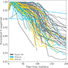 |
Fig. E.1. V-band light curves of our sample objects. The gray curves correspond to the "continuous" sample, the blue curves to the subgroup objects, and the yellow curves to the objects that are similar to 2023ixf in their spectral appearance. The light curves have been normalized to their peak or maximum observed brightness to better visualize differences. |
All Tables
All Figures
|
Fig. 1. Example of the LOWESS-based continuum removal applied to selected spectra of SN 2012aw. Top left: Original spectra with the LOWESS-smoothed continuum overplotted. The yellow marker indicates a reference wavelength at which the local linear fits are displayed for each spectrum. The blue shaded region highlights the masked Hα feature, excluded from the continuum fitting to avoid bias Bottom left: Shape of the LOWESS kernel at the reference wavelength, illustrating the weighting scheme used during smoothing. Right: Continuum-normalized spectra obtained by dividing the original data by the LOWESS continuum fit. |
| In the text | |
|
Fig. 2. Gaussian process denoising applied to example spectra of SN 2015bs. The left plot shows the original spectra overlaid with their denoised counterparts, demonstrating the effectiveness of the procedure in preserving spectral features. The right panel shows histograms of the flux residuals attributed to noise. The near-Gaussian distribution of these residuals supports the assumptions of white noise and confirms that no significant correlated features were removed during the process. |
| In the text | |
|
Fig. 3. Illustration of the Gaussian process-based interpolation of the spectral time series. Panel (a) 3D view of the continuum-normalized spectral time series of SN 2007od interpolated onto a common time–wavelength grid. Panel (b) projection of panel (a), collapsed along the time axis, highlighting the evolution of spectral changes in the region around Hα. Panel (c) flux evolution at a given wavelength bin (red dashed line in panels (a) and (b)), with GP fit color-coded by epoch. |
| In the text | |
|
Fig. 4. PCA results at one representative epoch. The figure shows the PCA applied to continuum-normalized spectra at 20 days post-explosion. The top spectrum represents the mean SN II spectrum at that epoch, while the spectra below show the first few eigenspectra derived from the PCS (via singular value decomposition, SVD), ordered from top to bottom by decreasing significance. For reference, the mean spectrum is overplotted in light gray behind each eigenspectrum. The numbers next to each eigenspectrum indicate the corresponding eigenvalue, which reflects the variance explained by that PC. The inset plot in each panel displays the eigenvalue decay, indicating the variance captured by each component. |
| In the text | |
|
Fig. 5. t-SNE projection plots of the PCA coefficients (per epoch). These plots show how the SNe are distributed within the high-dimensional PCA space after dimensional reduction. Colored pentagons mark the positions of different CMFGEN models variants. SNe 2023ixf and 2024ggi are also added using the spectra currently available in the literature (red crosses), along with CSM-interacting SNe II from Jacobson-Galán et al. (2024) (green stars). A clear separation by s2 values is observed across all epochs, confirming the link between spectral and light curve properties. At 50 days, two groups emerge: a continuous “regular SNe IIP/L” sequence along s2, and a scattered subgroup, likely shaped by strong CSM interaction (marked by the yellow rectangle). Model projections align with expectations: CSM-rich models explain the subgroup objects, while mass-loss models resemble fast-declining SNe. |
| In the text | |
|
Fig. 6. Comparison between the day 20 and day 30 interpolated spectral features of 2023ixf and 2024ggi with the nearest models from Hillier & Dessart (2019), based on Fig. 5. |
| In the text | |
|
Fig. 7. Cornerplot of the measured spectral and light curve parameters for our supernova sample (blue and yellow squares together) at the epoch of 50 days. The blue circles represent the supernovae that belong to the “continuous” subclass of SNe II, while the yellow squares are the objects that are members of the detached subgroup based on their spectral appearance and the clustering performed in Sect. 4.3. The red circles represent the measurements done in Gutiérrez et al. (2017b), for comparison. The τ values are the Kendall-tau correlation parameters for the canonical SNe. |
| In the text | |
|
Fig. 8. Top: Median reconstructed spectral trends as a function of the s2 light curve decline rate based on our PCA analysis. The four sets of spectra correspond to the four investigated epochs. The color of the individual spectra shows the s2 light curve decline rate for which they were calculated. Bottom: Subgroup spectra. The gray spectra show those of the subgroup objects (defined by Fig. 5, the blue spectra show their median for each epoch. The red dashed spectrum shows the reconstructed spectrum for s = 2.5 [mag/100 d] (which is the darkest red spectrum on the left-hand side plot), while the black curve shows the spectra of SN 2023ixf. |
| In the text | |
|
Fig. A.1. PCA solution for the 30-day epoch spectra without denoising them in advance. The overall trends and the individual principal components match well those obtained in the run with the applied denoising. The main difference is the lower significance of the PC-s due to the more excessive noise terms that also enter the higher-order components, meaning that more components are necessary for a more reliable decomposition. |
| In the text | |
|
Fig. A.2. Recovered spectral features along changes in the light curve decline rate without the use of prior denoising on the spectra. The change in the features along the light curve decline rates matches that presented in Fig. 8: for more significant decline rates, one finds more suppressed emission and absorption lines. |
| In the text | |
|
Fig. B.1. Spectral differences of IIP and IIL supernovae. The rows correspond to the spectra before and after the continuum normalization. The columns, from left to right: the full sample, the subsample of IIL type supernovae (exhibiting light curve decline rates larger than 1.5 mag / 100 d), and the subsample of IIP supernovae with lower decline rates. The bold colored lines show the medians of the subsamples. |
| In the text | |
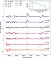 |
Fig. C.1. Same as Figure 4, but at 40 days post-explosion. |
| In the text | |
|
Fig. E.1. V-band light curves of our sample objects. The gray curves correspond to the "continuous" sample, the blue curves to the subgroup objects, and the yellow curves to the objects that are similar to 2023ixf in their spectral appearance. The light curves have been normalized to their peak or maximum observed brightness to better visualize differences. |
| In the text | |
Current usage metrics show cumulative count of Article Views (full-text article views including HTML views, PDF and ePub downloads, according to the available data) and Abstracts Views on Vision4Press platform.
Data correspond to usage on the plateform after 2015. The current usage metrics is available 48-96 hours after online publication and is updated daily on week days.
Initial download of the metrics may take a while.