| Issue |
A&A
Volume 708, April 2026
|
|
|---|---|---|
| Article Number | A244 | |
| Number of page(s) | 20 | |
| Section | Extragalactic astronomy | |
| DOI | https://doi.org/10.1051/0004-6361/202557624 | |
| Published online | 08 April 2026 | |
The baryon budget of galaxies across the first billion years
Theoretical predictions for gas phases, depletion times, stellar return fractions
1
INAF-Italian National Institute of Astrophysics, Observatory of Trieste, Via G. Tiepolo 11, 34143 Trieste, Italy
2
Institute for Fundamental Physics of the Universe, Via Beirut 2, 34151 Trieste, Italy
3
European Southern Observatory, Karl-Schwarzschild-Straße 2, 85748 Garching bei Muenchen, Germania
4
Aix Marseille Université, CNRS, LAM (Laboratoire d’Astrophysique de Marseille) UMR 7326, 13388 Marseille, France
★ Corresponding author: This email address is being protected from spambots. You need JavaScript enabled to view it.
Received:
9
October
2025
Accepted:
15
February
2026
Abstract
Context. ALMA and JWST observations of galaxies in the first billion years of the Universe provide key constraints on the baryon cycle during the epoch of reionisation. A complete census of the baryonic phases in early galaxies is essential to understand the efficiency and timescales of star formation.
Aims. In this work, we study cosmic matter at redshift z > 5 to investigate the different phases in which early gas and stars reside, their corresponding mass budgets, the resulting depletion times, and the expected stellar return fraction as a function of stellar age.
Methods. We used the COLDSIM hydrodynamical time-dependent non-equilibrium chemistry simulations to perform a detailed analysis of the cold, warm, hot, and stellar phases for both bound structures (galaxies and their circumgalactic medium) and the diffuse intergalactic medium. We further investigated the cold HI and H2 components, explicitly computed in our simulations, and examined their relations with the host mass, star formation, metallicity, and depletion timescales. We also provide observational insights and discuss the implications for stellar mass functions, Population III star formation, and changes in the initial mass function.
Results. Cosmic gas prior to reionisation is mostly cold, while at later epochs the warm phase becomes dominant as a consequence of enhanced star formation activity and increasing UV reionising radiation. Stellar return fractions at these times are ∼0.15–0.20, a factor of two lower than the values usually adopted. Mass functions and mass density parameters in bound objects increase with cosmic time, closely tracing the overall structure formation process. Cold, warm, and hot gas masses as well as HI and H2 components show increasing trends with mass and star formation rate, while HI and H2 depletion times decrease down to 0.01–0.1 Gyr with a weak dependence on metallicity. The resulting star formation efficiency remains at the level of a few percent independently of z and gas-to-star fractions decline with mass, influenced by local feedback and environment. Our findings are consistent with ALMA, VLA and IRAM surveys at later epochs, including ALFALFA, xCOLDGASS, GASS, xGASS, EDGE-CALIFA, PHIBBS, and ASPECS.
Conclusions. Gas phases are quantitatively related to the underlying stellar populations and can be used to infer unknown quantities. In the appendix, we provide fit functions describing the trends of the stellar return fraction, the main sequence, phase mass relations, gas-to-star fractions, and depletion timescales.
Key words: galaxies: formation / galaxies: high-redshift / intergalactic medium / galaxies: star formation
© The Authors 2026
 Open Access article, published by EDP Sciences, under the terms of the Creative Commons Attribution License (https://creativecommons.org/licenses/by/4.0), which permits unrestricted use, distribution, and reproduction in any medium, provided the original work is properly cited.
This article is published in open access under the Subscribe to Open model. This email address is being protected from spambots. You need JavaScript enabled to view it. to support open access publication.
1. Introduction
Baryonic structure formation relies on a scenario in which cosmic gas falls into the galaxy potential wells from large scales, cools down, and condenses into stars. Formed stars release energy and mass into the surrounding medium via star formation feedback that, together with active galactic nucleus (AGN) activity, leads baryon outflows. This determines a continuous mass transfer among different baryon phases and scales, during which matter flows in and out of galaxies: the so-called baryon cycle (e.g. Tumlinson et al. 2017; Péroux & Howk 2020). This latter essentially mediates the interplay between cosmic mass that is gravitationally bound in galaxies and the intergalactic medium (IGM). Primordial times witness the very first episodes of the cosmic baryon cycle, which is likely in place by the first half-gigayear of the Universe.
Recent JWST and ALMA detections (Bañados et al. 2024; Chemerynska et al. 2024; Carniani et al. 2024; Huertas-Company et al. 2025; Schouws et al. 2025a,b; Helton et al. 2025a; Naidu et al. 2026; Conselice et al. 2025; Fujimoto et al. 2025; Gandolfi et al. 2025) suggest that the first galaxies have already formed by redshift z ≃ 14 and present relatively complex metallicity (Z) patterns with a star-forming main sequence established over timescales of 10–100 Myr. The onset of such early star formation episodes requires significant amounts of cold molecular (H2) mass. Indeed, neutral hydrogen (HI) and helium are not efficient coolants below about 104 K, but HI and residual free electrons trigger the formation of large quantities of H2 both in pristine population III (PopIII) and in polluted population II-I (PopII-I) regimes (Saslaw & Zipoy 1967; Hollenbach & McKee 1979; Abel et al. 1997; Galli & Palla 1998; Maio et al. 2010; Wise et al. 2012; Huyan et al. 2025; Vanzella et al. 2026).
Cold or cooling gas is commonly observed in galaxies through HI 21 cm line or molecular transitions. Warm gas is usually seen in star-forming sites via photoionisation emission in Hα or high-ionisation metal species and expected in optically thick regions of MHD-driven accretion discs. With high-energy instruments, such as eRosita or XRISM, hot (2–10 keV) gas can be found in optically selected objects at z ≃ 0–2, X-ray emitting galaxy clusters, and AGN coronas (Jiang et al. 2019; Comparat et al. 2023). Resolved active-galaxy studies in the local Universe have detected kiloparsec-scale molecular outflows with strong contributions from the H2 phase at temperatures of T ≳ 103 K (Cicone et al. 2014, 2021; Lamperti et al. 2022; Zanchettin et al. 2025; Koribalski et al. 2025; Langan et al. 2026), while MUSE observations indicate the presence of ∼102 K molecular gas in galaxies that are both accreting and expelling material (Weng et al. 2022). Despite the evidence that baryons can be found in a broad variety of phases and objects, quantitative estimates are challenging.
The relations between cold neutral gas (detected in absorption) and warm ionised gas (probed in emission) are currently being explored. Recent comparative studies involving controlled samples at z ≃ 2–4 have found a typical variance in the probed gas abundances of 0.2-0.3 dex with dependencies on the line diagnostic used (Schady et al. 2024). This approach opens the possibility of combining both absorption and emission techniques to better investigate high-z faint galaxies (Kulkarni et al. 2022). Nevertheless, theoretical studies focusing on high-z gas phases are still lacking and the contribution of cold, warm, and hot gas to the whole cosmic mass budget is to be determined.
It is known from both observational results and theoretical calculations that at z < 6, after reionisation completes, the cosmic mass density of cold neutral gas flattens around 10−3 of the cosmic critical density (Wolfe et al. 1995; Rao & Turnshek 2000; Storrie-Lombardi & Wolfe 2000; Péroux et al. 2001; Nagamine et al. 2004; Tacconi et al. 2020; Heintz et al. 2022). The condensed baryon budget is dominated by the HI component, while corresponding H2 values are estimated to be much lower (between a factor of a few and some dex; Walter et al. 2020; Decarli et al. 2020; Maio et al. 2022; Boogaard et al. 2023; Messias et al. 2024). Previous studies have shown that warm or hot gas can account for a large fraction of baryons in low-redshift structures (e.g. Dev et al. 2024; Deepak et al. 2025), but at high z the situation is extremely uncertain and their share, distribution, and evolution is debated (Peroux & Nelson 2024).
The interplay among different gas phases, the conversion of cold gas into stars and the release of stellar mass into warm and hot gas depend on a few physical quantities, i.e. gas depletion times (tdepl), stellar ages (tage), and the stellar return fraction (R). A clear assessment of these variables is crucial for our understanding of the early baryon cycle, as well as for addressing the connection between gas and stars. Low-z and cosmic-noon studies have suggested that typical depletion times might be of the order of some gigayears (Tacconi et al. 2013, 2018; Castignani et al. 2025; Kaur et al. 2025), while commonly adopted values for R are obtained by averaging over a chosen initial stellar mass function (IMF) and imposing instantaneous recycling of massive stars (Maeder 1992; Madau & Dickinson 2014). That means that stellar ages and time-dependent yields are not taken into account. Thus, resulting R values, typically in the range of R ≃ 0.3–0.4 for Salpeter (1955) and Kroupa (2001) or Chabrier (2003) IMFs, can be considered valid only on timescales of 5–10 Gyr. Due to the much shorter cosmic times at z ≳ 5, those findings are unreliable for such an epoch. Hence, depletion times and stellar return fractions should be revised and reconciled with high-z timescales. This is relevant for estimating stellar masses and star formation rates (SFRs) in the early Universe.
Throughout this work, we shed light on these issues by using ad hoc hydrodynamical simulations of primordial structure formation taken by the COLDSIM project (e.g. Maio et al. 2022; Casavecchia et al. 2024; Parente et al. 2026). We adopt a Λ cold dark matter (ΛCDM) model with present-day cosmological-constant, matter, and baryon density parameters of Ω0, Λ = 0.726, Ω0, m = 0.274, and Ω0, b = 0.0458, respectively. The expansion parameter normalised to 100 km/s/Mpc is h = 0.702, while the mass variance within 8 Mpc/h radius is σ8 = 0.816 and the power spectrum index is n = 0.968 (Planck Collaboration VI 2020). The comoving cosmological critical density is ρ0, crit = 277.4 h2M⊙ kpc−3 = 136.7 M⊙ kpc−3 and the value of the metallicity in the solar neighbourhood is Z⊙ = 0.02. All logarithms are in base 10.
The text is organised as follows. In Sect. 2, we describe the numerical simulations used and the analysis performed. In Sect. 3 we show our main results and in Sect. 4 we discuss them. We then summarise our findings and conclude in Sect. 5. Fitting relations and supplementary material are collected in the appendix.
2. Method
We employed the detailed and accurate COLDSIM numerical simulations of primordial cosmic structure formation. The implementation includes gravitational-force calculations and smoothed-particle hydrodynamics inherited from the P-GADGET-3 code (Springel 2005) and additional extensions including: non-equilibrium atomic and molecular chemistry (for e−, H, H+, H−, He, He+, He++, H2, H2+, D, D+, HD, and HeH+) explicitly followed in cold, warm, and hot gas phases; dust grain catalysis; photoelectric and cosmic-ray heating; HI and H2 density-dependent self-shielding; gas cooling from resonant and sub-millimetre fine-structure line emission; star formation and stellar evolution of PopII-I and PopIII stars according to a Salpeter IMF; remnant masses and metal spreading for He, C, N, O, Ne, Mg, Si, S, Ca, and Fe, from type-II and type-Ia supernovae (SNe) and asymptotic-giant-branch (AGB) events according to metal-dependent yields and lifetimes; thermal feedback; and galactic winds (kinetic feedback) at 350 km/s (Maio et al. 2022; Maio & Viel 2023; Casavecchia et al. 2024, 2025; Parente et al. 2026). PopIII and PopII-I regimes are differentiated in terms of a critical metallicity Zcrit = 10−4 Z⊙ and differ for the stellar metal yields adopted. Yields for zero-metallicity stars are used in the PopIII case (Z < Zcrit) and yields for metal-enriched stars in the PopII-I case (Z ≥ Zcrit). We remind the reader that Zcrit values are quite uncertain (Bromm et al. 2001a; Omukai et al. 2005; Santoro & Shull 2006; Chiaki et al. 2014; Chon et al. 2024), but, due to the rapid metal enrichment by early SNe, different assumptions do not lead to significantly different results (Maio et al. 2010).
We consider three cosmic volumes initialised at redshift z = 99 according to the ΛCDM paradigm. Our reference (Ref) set-up has a comoving box side of L = 10 Mpc/h and an initial number of gas and dark-matter particles of Npart = 2 × 5123. The high-resolution (HR) run has the same L, and Npart = 2 × 10003, while the large-box (LB) run is characterised by L = 50 Mpc/h and Npart = 2 × 10003. We performed our analysis on the Ref run and checked the effects of resolution or volume sampling by comparisons with the HR and LB simulations in Appendix A and B. The resulting gas (mgas) and dark-matter (mdm) mass resolutions are listed in Table 1.
Simulation set-up for the HR, Ref, and LB runs.
Cosmic structures were identified by searching for clustered particles via a friend-of-friend technique with a linking length of ∼0.2 the mean inter-particle separation. A substructure finder algorithm checked for minimal values of the local gravitational potential and gave us basic properties of gravitationally bound structures (Dolag et al. 2009), such as the position, virial radius (Rvir), virial mass (Mvir), stellar mass (Mstar), SFR, and Z. To avoid numerical artefacts that could have led to spurious results, we considered bound structures to be well behaved only if they were sampled with at least 300 particles and their Rvir > 0. A pictorial view of such cosmic objects is given in Fig. 1, where the projected mass-weighted temperature is shown for the most massive halo at z ≃ 6 traced back to z ≃ 10 and 14 when its total mass is 6.9 × 10¹⁰, 7.3 × 10⁹, and 1.4 × 10⁹ M⊙, and its physical virial radius is 18.7, 5.9, and 2.4 kpc, respectively. For all the simulated objects, we additionally evaluated the masses in the cold, warm, and hot gas phase defined as the ones with gas temperatures of T < 104 K, 104 ≤ T/K ≤ 107, and T > 107 K (Table 2). From the abundances derived by our chemistry network, we explicitly computed the HI and H2 masses, too. Our modelling produces a main sequence characterised by a rather flat specific-SFR (sSFR) trend with Mstar, in agreement with available observations (Appendix C). The simulated sequence at z > 5 can be fitted by
 (1)
(1)
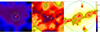 |
Fig. 1. Mass-weighted temperature maps at z ≃ 14, 10 and 6 smoothed on a grid of 1024 pixels a side for the gas in the largest halo that has a physical virial radius (circles) of ∼2.4, 5.9, and 18.7 kpc and a total mass of 1.4 × 10⁹, 7.3 × 10⁹, and 6.9 × 10¹⁰ M⊙, respectively, from left to right. |
Gas phase definitions.
and analogous relations hold at different z (Appendix C).
The resulting SFR density (SFRD) is in line with recent observational data, as shown in our previous works (e.g. Fig. 2 in Casavecchia et al. 2024), where resolution impacts for the Ref, LB, and HR runs are discussed, as well.
3. Results
In the next sections, we present our main results about the cosmic baryon census and the links among different mass phases. We first present global trends (Sect. 3.1), then we study the relations between baryon phases and galaxy properties (Sect. 3.2). Finally, we address the picture for the baryon cycle (Sect. 3.3).
3.1. Global trends
Mass density parameters and mass functions are shown below.
3.1.1. Mass density parameters
Baryon mass density parameters in the simulated cosmic volume were computed as: Ωphase = ρphase/ρ0, crit, with ρphase comoving mass density of the given baryonic phase considered (cold, warm, hot, stars, HI, H2).
Results for Ωcold, Ωwarm, Ωhot, Ωstars, ΩHI, and ΩH2 are shown in Fig. 2. From the trends it is clear that at z ≳ 6 the cold phase dominates the cosmic mass budget, with a mass density parameter that closely traces Ω0, b. At z ≲ 6, reionisation gets completed and Ωcold drops by almost two orders of magnitudes, stabilising around 10−3 (possibly linked to surviving neutral islands; Malloy & Lidz 2015; Becker et al. 2015; Bosman et al. 2018; Kulkarni et al. 2019; Nasir & D’Aloisio 2020; Gnedin & Zhu 2025; Becker et al. 2024; Spina et al. 2024; Zhu et al. 2024; Davies et al. 2026), while the warm component catches up and becomes the most important mass reservoir at later times. At early epochs, Ωwarm is driven by star formation feedback and its contribution is as low as ∼10−6 at z ∼ 20, about 5 dex smaller than Ωcold. Ongoing star formation heats up cold material and triggers the conversion of increasingly large amounts of cold gas into warm gas between z ∼ 20 and 6. This is reflected by the behaviour of Ωstars, which accounts for a fraction of a percent of the mass involved in star-forming events (as traced by the warm phase). We note that the stellar budget was derived from a Salpeter IMF and that possible IMF variations (Kroupa 2001; Chabrier 2003; Bell & de Jong 2001; Bell et al. 2003; Gallazzi et al. 2008; Herrmann et al. 2016; Blackwell et al. 2026) impact Ωstars by up to 0.3 dex (a factor of 2), as summarised in Table 3.
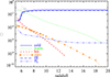 |
Fig. 2. Baryon density parameters as function of redshift for cold (solid line), warm (dotted line), hot (short-dashed line), stellar (dot-dashed line with asterisks), HI (long-dashed line), and H2 (dot-dot-dot-dashed line) phases. The horizontal grey line marks the value of Ω0, b. |
Impact of IMF variation on stellar masses.
Hot gas mass generated during cosmic structure assembly is subdominant, since it traces larger and rarer objects. The cold phase hosts both HI and H2, two crucial species for the conversion of gas into stars. While HI typically accounts for 3/4 the cold mass, H2 molecules are almost ubiquitous. Their production gets enhanced during the early gas collapse at z ∼ 15–20 and increases by roughly two orders of magnitudes by z ∼ 5.
3.1.2. Mass functions
Fig. 3 shows mass functions for cold, warm, and hot gas at z ≃ 5–16. The mass function is defined as the number of objects with a given (phase) mass per unit volume and per unit logarithmic mass bin. In all three cases, the mass function evolves from narrow, poorly sampled distributions (z ≃ 16) to broader and richer ones (z ≃ 5) with higher normalisation values towards lower redshifts. That is a direct consequence of cosmic structure formation, which causes an increase over time of the number density of formed galaxies. The cold and warm phases peak at Mcold ∼ Mwarm ∼ 107 M⊙ and the hot phase at Mhot ∼ 105 M⊙ at roughly any z. The high-mass end of the distributions show that the maximum values of cold, warm, and hot masses are very different, with Mcold reaching ∼ 109 M⊙, but Mwarm ∼ 1010 M⊙ and Mhot only ∼108 M⊙. Larger objects are able to retain larger amounts of baryons, while smaller objects have shallower potential wells, and hence are more susceptible to feedback energetics. A clear example is offered by the cold-phase mass distribution between z ≃ 6 and 5, when reionisation heats up cold, diffuse gas and leads to a decrease in the peak mass and the low-mass tail. At z ≳ 6 the redshift evolution is quite neat and regular and results from the interplay between local gas cooling and stellar heating. By comparing the masses of different gas phases at any fixed z, we find in general a minor role played by hot gas and a more relevant role played by cold and warm gas at most scales.
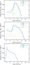 |
Fig. 3. Cold (top), warm (centre), and hot (bottom) gas mass functions at z = 5.25, 6.14, 8.09, 10.00, 13.01, and 16.01. |
Looking at the details of cold-mass distributions, in Fig. 4 we make predictions for the HI and H2 mass functions. The former closely follows the Mcold behaviour, as expected from its typical abundances (see Fig. 2); hence, the HI mass function is a reliable tracer of the cold-gas mass function. In the upper panel, we also show a fit derived by ALFALFA data and valid at z = 0 for MHI > 106 M⊙ (Jones et al. 2018). Clearly, the low-redshift trend is not a good description of the high-z HI distribution, when mass regimes and gas thermal states are rather different. In fact, the lack of early, grown, massive structures biases the resulting high-z HI distributions towards values of MHI < 109 M⊙. Halo mass growth and/or mergers at later times are expected to shift HI masses up to MHI ≃ 1010–1011 M⊙ and reionisation would lower the abundance of smaller (mostly unshielded) objects with MHI ∼ 106–108 M⊙. The behaviour of the H2 mass function is more convolved, because MH2 can grow in a variety of temperature and density regimes and both stellar feedback and reionisation are efficient at dissociating unshielded H2 mass. In particular, the high-MH2 end is driven by molecular formation in thick cooling gas, while the low-mass tail is determined by H2 destruction due to stellar feedback (z > 6) or reionisation (z ≲ 6).
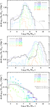 |
Fig. 4. HI (top), H2 (centre), and stellar (bottom) mass functions at different z with a fit to z = 0 ALFALFA HI data by Jones et al. (2018) (top panel, dotted grey line), z = 6–10 HST/Spitzer masses by Stefanon et al. (2021) (bottom panel, coloured crosses) and expectations by Jaacks et al. (2019) (bottom panel, coloured diamonds). |
The mass distribution of the young (tage < 100 Myr) stellar component is plotted in the bottom panel of Fig. 4 and compared with UV-based determinations for z = 6–10 HST and Spitzer galaxies (Stefanon et al. 2021). The resulting trend decreases with Mstar and follows a Schechter form, while redshift evolution is evident in the normalisation and reflects the level of star formation activity from early to late times. A plethora of previous works have shown stellar mass functions, such as those in the bottom panel of Fig. 4. Nevertheless, the low-mass regime is still debated and more observational data of faint or normal star-forming galaxies at those epochs are needed to draw definitive conclusions. Broadly speaking, we find a power-law trend down to Mstar ∼ 106 M⊙ and a flattening of the distribution at lower Mstar, while the high-mass regime is in line with the data by Stefanon et al. (2021). Independent theoretical results by Jaacks et al. (2019), despite focusing on a smaller-mass range, find a behaviour that is qualitatively similar to ours (although steeper at z ∼ 8), with a mild flattening around Mstar ∼ 105-106 M⊙. The existing discrepancies could be ascribed to the different stellar-population assumptions, selection effects, or numerical resolution. As is noted therein, the flattening values correspond to the transition between (smaller) H2-cooling haloes and (larger) H-cooling haloes, with implications for cooling efficiencies. Thus, gas cooling is key for the establishment and shape of the early stellar mass function.
3.2. Baryon budget, galaxies and the IGM
We explore where different baryon phases are located and their relations with the hosting environment by looking at the mass density parameters in bound structures and in the IGM, as well as their possible correlations with the main galaxy properties.
3.2.1. Mass phases in bound structures and IGM
Mass density parameters in bound structures and the IGM were estimated by selecting the total mass within a distance of R < Rvir from halo centres (Ωbound) and the mass lying beyond any Rvir (ΩIGM) for each phase. The selected bound mass therefore included both galaxies and their circumgalactic medium (CGM). The share of cold, warm, hot, stellar, HI, and H2 mass phases in bound structures (Ωbound, cold, Ωbound, warm, Ωbound, hot, Ωbound, stars, Ωbound, HI, Ωbound, H2) and diffuse gas (ΩIGM, cold, ΩIGM, warm, ΩIGM, hot, ΩIGM, stars, ΩIGM, HI, ΩIGM, H2) are presented in Fig. 5, while corresponding bound-to-cosmic and IGM-to-cosmic mass density ratios are in Appendix D.
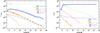 |
Fig. 5. Baryon density parameters in bound objects (left) and the IGM (right) as function of redshift for cold (solid lines), warm (dotted lines), hot (short-dashed lines), stellar (dot-dashed lines with asterisks), HI (long-dashed lines), and H2 (dot-dot-dot-dashed lines) phases. The horizontal grey line marks the value of Ω0, b. Stars form out of cold gas that dominates the baryon budget at z ≳ 6 and is overtaken by warm gas at later times. |
The trends for bound objects follow the halo growth during cosmic evolution with little amounts of mass in bound structures at early times and increasingly large amounts of bound mass at later epochs. This is particularly evident for Ωbound, warm, Ωbound, hot, and Ωbound, stars that increase monotonically with time and signal the build-up of gaseous and stellar content in galaxies. The trend of Ωbound, cold is affected by reionisation at z ≃ 6, when the UV background radiation ionises HI (Ωbound, HI drops) and slightly boosts H2 in the thin regions of halo peripheries (Ωbound, H2 gets enhanced). This causes Ωbound, warm to dominate the baryons in collapsed structures at z < 6. When compared to the whole cosmic mass, the resulting Ωbound values are different from those in Fig. 2 and discrepancies reach a few dex (consistently with the phase average evolution shown in Appendix D, Fig. D.2).
For the diffuse gas, the values of ΩIGM, cold, ΩIGM, warm, and ΩIGM, hot tightly follow the corresponding Ωcold, Ωwarm, and Ωhot cosmic behaviour and the picture arising from Fig. 5 is similar to the one of Fig. 2. In the IGM case, the stellar phase is negligible, as primordial stars are typically formed in bound structures (early galaxies). While HI traces IGM cold gas well, H2 features a resulting ΩIGM, H2 ∼ 10−6 at z ≃ 18 (in line with primordial abundances) and ΩIGM, H2 ≳ 10−5 at z < 6.
3.2.2. Phase relations
It is debated whether gas phases correlate with the main galaxy properties and if they could be used to infer unknown quantities.
To address these questions, we check gas scaling relations in Fig. 6, where cold, warm and hot gas masses in bound structures are plotted against the hosting Mstar (upper row) and SFR (lower row). Corresponding mass fractions are shown in Appendix D. To better guide the eye, we overplot fits to simulation results, as reported in Appendix F. Gas phase masses generally increase with Mstar and SFR and the results in the figure show that the hot component is subdominant by a factor of ∼102–103 at all z. Warm and cold phases share comparable amounts of mass with slightly more cold gas in smaller systems (Mstar ≲ 107 M⊙). The trend is shallower for the cold material and steeper for the warm one (which dominates at SFR ≳ 0.01–0.1 M⊙). Simulation results suggest that cold, warm and hot gas masses increase with both Mstar and SFR with slopes of ∼0.2, 0.5 and 0.6 (Table F.1).
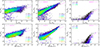 |
Fig. 6. Cold (left column), warm (central column), and hot (right column) gas mass versus Mstar (top row) and SFR (bottom row) for galaxies at redshift z = 5.25, 6.14, 8.09, 10.00, 13.01, and 16.01, with simulation fits (dashed magenta lines) reported in Appendix F (Table F.1). Different gas phases probe different Mstar and SFR regimes with little redshift evolution, but a large environment and feedback-driven scatter. |
We further explore the trends of HI and H2 masses as functions of Mvir, Mstar, and SFR in Fig. 7. We compare our predictions with z ∼ 0 HI data from HIPASS and ALFALFA surveys (Padmanabhan & Kulkarni 2017; Guo et al. 2021) and with H2 data from ALMA/NOEMA surveys of star-forming galaxies at z ∼ 1–3 (Bertola et al. 2024), nearby DustPedia galaxies (Salvestrini et al. 2025), and MUSE-ALMA galaxies (Bollo et al. 2026). HI and H2 mass relations feature little evolution and the scatter broadens due to both larger sample statistics and increasing feedback impacts at lower z. Their scalings with Mstar and SFR are similar, consistently with the main-sequence relation at this epoch, and are characterised by slopes of roughly 0.2 and 0.5 (Table F.2). The H2 behaviour is in agreement with recent MUSE-ALMA upper limits at z ≃ 0.5 by Bollo et al. (2026) and the fundamental plane by Salvestrini et al. (2025), whose multi-parametric fit suggests an MH2-SFR slope of 0.51 at z ≃ 0 (see also Sargent et al. 2014). Low-z observations are qualitatively in line with our predictions, although they bear remarkable uncertainties (Romeo 2020; Romeo et al. 2020; Chowdhury et al. 2022; Bianchetti et al. 2025).
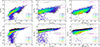 |
Fig. 7. HI (top) and H2 (bottom) masses versus Mvir (left), Mstar (centre), and SFR (right). Observational fits for HI and H2 data are shown by grey dotted lines and MUSE-ALMA Haloes H2 upper limits (Bollo et al. 2026) by grey circles and arrows. The fit to the MUSE-ALMA Haloes MHI vs. Mstar is Log(MHI/M⊙) = 0.50 Log(Mstar/M⊙)+4.52 (O’Beirne et al. 2026, priv. comm.) and is extrapolated from galaxy data at Mstar ∼ 108–1012 M⊙. Multi-parametric fits by Salvestrini et al. (2025) are shown for SFR = 10−1 M⊙ yr−1 (lower central panel) and Mstar = 108.5, 107, and 105.5 M⊙ (dotted lines from top to bottom in the lower right panel). Simulation fits (dashed magenta lines) are in Appendix F (Table F.2). Results are little dependent on redshift and feature a large environment-driven scatter. |
Supplementary material about HI and H2 total gas fractions fHI and fH2 versus Mvir, Mstar, SFR, and Z is given in Appendix D. Here, we only stress that, due to feedback effects, fHI may reach values ≲0.1 of the whole gas mass (in objects dominated by warm or hot gas), while fH2 is typically around a few percent, but reaches values larger than 10% in cold, metal-enriched, star-forming sites. Finally, we checked the relations between gas phases and metallicities and found that they are similar to the ones in Figs. 6 and 7 because of the mass-metallicity relation.
3.3. Baryon cycling: Connecting gas and stars
Baryon phases are influenced by both the stellar activity – that returns a fraction of stellar mass to the gaseous environment during stellar evolutionary stages (stellar return fraction; R) – and the efficiency with which gas is converted into stars during a typical depletion time (star formation efficiency; SFE). These two phenomena are signposts of the interaction between gas and stars and we quantify them in the next section.
3.3.1. Stellar return fraction
The stellar return fraction, R, depends on the assumed stellar IMF, metal yields, mass loss during SN explosions and AGB winds, stellar remnants, and stellar lifetimes. Most authors rely on IMF-integrated averages of R, although this can vary for different populations and metallicities. Since in our simulations we track the stellar age (tage) of each population and the respective chemical enrichment and mass losses, here we improve on previous estimates by computing R self-consistently at different times for multiple stellar populations. For each output, the average return fraction is R = 1 − Ωstars/Ω0, stars, with Ωstars and Ω0,satrs current and initial stellar mass density parameters.
Fig. 8 shows the resulting average trend for R(tage) at z = 5, 12, and 18, fitted as a function of tage as follows:
 (2)
(2)
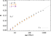 |
Fig. 8. Stellar return fraction R as a function of stellar age for simulated data at redshifts z = 5 (crosses), 12 (diamonds), and 18 (triangles) in the Ref run. Data points refer to median R values with median absolute deviation, while the solid grey line is the corresponding fit (Eq. 2). |
if tage > 3.853 Myr and R = 0 otherwise. We note that, at tage ≃ 10 Gyr, R ≃ 0.3, consistently with the expectations for a Salpeter IMF.
Our results imply that in high-z galaxies the amount of stellar mass that is released into the surrounding gas is smaller than the amount inferred by common IMF-integrated estimates. Our z = 5 figures are around 0.15–0.20, i.e. half of the typically adopted values. This is a consequence of the younger ages in high-z populations that have had not enough time to evolve through all the stellar stages and eject large amount of mass back to the surrounding environment. These considerations suggest that the recycled material affects the baryon budget by a fraction of ≲20% at z > 5 and, since gas phases influenced by star formation feedback are predominantly warm, the corresponding Ωwarm values (in e.g. Fig. 2) would share such recycled baryons at the time of their ejection. On the other hand, early SN and AGB events (that take place on timescales of up to a few hundreds million years) seem efficient at boosting R to levels that are only a factor of two away from late-time expectations. These findings are not severely affected by metallicity effects (Appendix A) and impact available high-z SFRDs, which appear to suffer from R mis-estimates on top of IMF uncertainties (in Table 3).
3.3.2. Gas depletion and star formation
Depletion times effectively quantify the timescales needed to transfer mass from the cold HI and H2 phases to the stellar phase and are defined as: tdepl,HI = MHI/SFR and  .
.
In Fig. 9, the average HI depletion time presents an evolution from tdepl, HI ∼ 10 Gyr at z ∼ 20 to about 1 Gyr at z ∼ 5. Mean and median values are larger, at variance with the typical Hubble times at those epochs. The values for tdepl, H2 lie around ∼0.01–1 Gyr at z ∼ 5–20. They are shorter than the Hubble time at the same epochs and support the formation of bursty objects at z ∼ 15 and beyond. Mean and median values may differ from simple averages by a factor of a few up to one dex, as is shown in the figure. As a reference, the fitting expressions for the median HI and H2 trends at z≃5–20 are
 (3)
(3)
 (4)
(4)
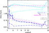 |
Fig. 9. Redshift evolution of average (regular lines), mean (thin lines), and median (thick lines) HI and H2 depletion times compared to dynamical time, tdyn (dotted black line), and observational expectations by Bollo et al. (2026) at low z (crosses with 1σ dispersion) and Péroux & Howk (2020) at z≃5–6 (diamonds with 1σ dispersion). Simulation fits (Appendix F) are overplotted with long-dashed magenta lines. |
The latter roughly follows the dynamical time of density contrasts Δ ≃ 500,  , with tH Hubble time (Fig. 9). Fits for average and mean evolution are in Appendix F.
In Fig. 10, tdepl, HI and tdepl, H2 are plotted as functions of SFR (further relations with Mstar, gas Z, and sSFR can be found in Appendix E). Their trend decreases as a result of ongoing star formation activity. In particular, the bulk of tdepl, H2 values are about 0.01–0.05 Gyr at z ≃ 16 and about 0.1–1 Gyr at z ≃ 6. Minimum values are reached in larger (Mstar ≳ 108 M⊙), more star-forming (SFR > 0.1 M⊙ yr−1) structures where typical gas metallicities are Z > 0.01 Z⊙. Because of the H2 sensitivity to star-forming processes, the tdepl, H2 scatter is broader than tdepl, HI and is due to environment and feedback episodes that alter gas molecular content and cooling capabilities in a non-trivial way. HI trends at different redshifts feature resulting normalisations that are higher by one or two dex. Fits to simulation results demonstrate that HI and H2 depletion times decrease with SFR (stellar mass) with slopes of −0.7 and −0.5 (−0.6 and −0.3), respectively (Table F.3).
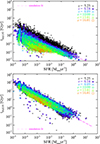 |
Fig. 10. H2 (top) and HI (bottom) depletion times versus SFR at z = 5.25, 6.14, 8.09, 10.00, 13.01, and 16.01 with simulation fits (Appendix F, Table F.3). Further trends with galaxy properties are in Appendix E. |
In Fig. 11 the median HI and H2 depletion times versus gas metallicity are displayed for the whole redshift range as well as for the different z considered in one-dex metallicity bins. The figures show neatly that average trends are decreasing with gas metallicity as a consequence of more efficient star formation in metal-rich environments. The difference between the average tdepl, HI and tdepl, H2 is almost three dex at Z ≲ 0.001 Z⊙ and one dex at Z ≳ 0.1 Z⊙. This suggests that metals are efficient in lowering tdepl, HI, although they are less crucial for tdepl, H2.
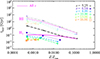 |
Fig. 11. Median HI (thin symbols) and H2 (thick symbols) depletion times vs Z at different z (coloured symbols) and for the whole z range (solid magenta lines). Gas metallicity affects depletion times at all z. |
Gas timescales allow us to infer the SFE of a given object, tff/tdepl, with tff and tdepl gas free-fall time and depletion time (Fig. 12, top panel). We find a median SFE ∼ 0.01–0.04, and values of around 0.1 for more star-forming objects (SFR > 0.01 M⊙ yr−1). This is in agreement with low-z data (Ni et al. 2025) and the lack of evidence for increased SFE at early times (Zavala et al. 2019; Donnan et al. 2025).
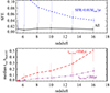 |
Fig. 12. Top: Median SFE redshift evolution with 1σ spread (top) for all (solid line) and star-forming (short-dashed line) objects. Bottom: Median trec/tdepl, H2 ratios with 1σ spread for trec, low = 9 Myr (long-dashed line) and 3 Myr (dot-dashed line) lower limits. |
Another interesting timescale is the recovery time, trec, which gives the time needed for gas to cool again after being heated by stellar feedback during the initial stages of star formation. We check its role in describing star-forming events in the lower panel of Fig. 12. The values of trec are functions of SN mass or, equivalently, lifetime (tage), and in Appendix F we provide fits to the results by Jeon et al. (2014) in the range of trec ∼ 9–300 Myr for 15–200 M⊙ SN explosions hosted in a halo with mass 5 × 10⁵ M⊙. We adopt the mentioned trec–tage fit in Appendix F and estimate median values of trec/tdepl, H2 for the simulated galaxy population. To bracket uncertainties about trec lower values (trec, low), we consider both 9 Myr and 3 Myr for trec, low (in line with Table 1 in Jeon et al. 2014) when using our fit. We find that trec behaves as a good tracer of the initial episodes of star formation in molecular gas, when it accounts for roughly 20–50% of the H2 depletion time (z ≃ 16); however, ongoing feedback effects make its contribution drop down to 1–10% at z ≃ 5–6.
4. Discussion
This paper presents an analysis of the baryon phases at the epoch of reionisation and, as for any research work, the obtained results may depend on the model assumptions performed, but also give hints as to how to interpret observational findings.
4.1. Model assumptions
We considered star particles as simple stellar populations described by a Salpeter IMF, although different choices are possible due to uncertainties in the sampling of low-mass, long-lived stars (see Table 3). We included energy ejection and mass loss from type-II SNe, low-mass stars and intermediate-mass stars. We accounted for type-Ia SNe by considering the classical (favoured) single-degenerate scenario (Whelan & Iben 1973), in which they form in binary systems after a delay of ∼0.1 Gyr and about 50% of them explode within 1 Gyr, irrespectively of the exact delay time distribution (Iben & Tutukov 1994; Greggio 2005; Cappellaro et al. 2015; Maoz & Graur 2017). The properties of the resulting population might depend on the inclusion of stellar rotation and post-zero-age-main-sequence evolution at high z, though (Hassan et al. 2025).
Gas cooling takes place via resonant, fine-structure, and molecular lines and is responsible for the transition from hot to warm and cold phases (Maio et al. 2007, 2010), while winds are generated within the smoothing kernel of star-forming particles with a constant velocity of 350 km/s and are decoupled from hydro calculations after their ejection in overdense regions (e.g. Maio et al. 2011a). Different wind implementations could potentially affect the gas located near star-forming sites, but the impacts should be limited as long as wind velocities are kept in realistic ranges, of around a few 102 km/s, and mass loading factors do not exceed extreme values of ∼5 (Perrotta et al. 2024).
We checked resolution effects and found that there can be differences in the warm, hot, and stellar phases, but the resulting trends are similar within one dex or less (Appendix A). This finding is related to the optimal gas resolutions adopted here which allow us to resolve gas phases at scales from megaparsecs to tens of parsecs at z ≳ 10. This is consistent with previous works (Creasey et al. 2011) that demonstrated that numerical overcooling can severely affect results for particle gas masses higher than ∼106 M⊙. We selected objects by means of their virial mass and number of constituting particles in order to exclude tiny, poorly resolved structures. Different selection criteria (explored in Appendix B) might lead to slightly different results; however, the general trends are preserved.
The temperature thresholds to distinguish cold, warm, and hot gas phases are somewhat arbitrary; however, most literature studies follow the choices we perform here. A typical threshold of 104 K is common in observational investigations to study neutral and HI gas masses at different redshifts (Nelson et al. 2020), while the threshold between warm and hot gas is debated and typically ranges between a few 106 K and 107 K. Here we chose 107 K and note that the impacts of adopting slightly lower values would be limited, due to the large amount of warm mass that dominates over hot gas.
We identified bound and IGM baryons by means of the virial radius. Alternative criteria might impact the final outcomes.
Our results for cosmic mass density parameters demonstrate that cold gas is the main baryon phase until reionisation, when its contribution drops down to Ωcold ∼ 10−3 and warm gas takes over. Of course, the details of this transition may depend on the reionisation history, the UV-background model adopted, and assumptions about heating and chemistry rates (Maio et al. 2022). Radiative-transfer effects of the radiation that escapes primordial star-forming regions might have an impact on the actual atomic and molecular abundances, since UV and Lyman-Werner photons might dissociate them in unshielded regions. Due to their rarity, primordial, solar-like, or OB-star sources do not induce dramatic variations in the average HI and H2 content over megaparsec scales (as quantified in Maio et al. 2016).
The sSFR trends we find are in line with observational data (Appendix C); however, caution must be taken when comparing numerical models with observations that may rely on different assumptions about the galaxy main sequence. We neglect primordial black-hole feedback, since in typical conditions its effects are expected to be minor due to the small galaxy masses at these epochs (see further discussion in e.g. Maio et al. 2019).
With these assumptions, our star formation efficiencies are of the order of a few percent, while average stellar return fractions are R ≲ 0.2 at the epoch of interest here (i.e. up to 20% of the initial stellar mass is converted into warm gas). As a consequence, any small fraction of cold gas that forms stars competes with increasing fractions of stellar mass turned back into gas via direct mass loss. These quantities affect the mass transfer from a phase to another; hence, different modelling or theoretical uncertainties of such processes might impact our findings.
We stress that the main thing responsible for the transition of gas from cold to warm or hot phases is not the mass transfer itself, which is quantitatively rather small, but the heating energy produced and injected into the surroundings after such small amounts of gas have formed stars. This happens via SN explosions and feedback, and the differentials of the curves in Figs. 2 and 5 give a quantitative measure of the actual mass transfer. These physical processes lead the mass flows among different phases, determining the complete baryon cycle.
4.2. Model variations and implications for the early SFRD
The primordial IMF is particularly debated in the literature (e.g. Palla et al. 1983; Silk 1983; Bromm et al. 2001b; Abel et al. 2002; Tornatore et al. 2007; Maio et al. 2010; Bromm 2013; Liu & Bromm 2020; Klessen & Glover 2023, and references therein) and a top-heavy shape is commonly adopted for PopIII regimes, following prescriptions by Larson (1998). His argument was based on the higher Jeans (Bonnor-Ebert) masses expected at higher redshift, due to the increasing cosmic-background temperature. Subsequent studies have highlighted the role of further physical processes, such as local gas shielding, partial recombination, magnetic fields and binary or cluster formation, which would bring proto-stellar seed masses down to values comparable to solar and following a power-law (unbiased) distribution (Yoshida et al. 2007; Clark et al. 2011; Greif et al. 2011; Hirano et al. 2014; Stacy et al. 2022; Chon et al. 2022; Machida et al. 2025; Gjergo et al. 2026). Direct evidence is not available yet, and thus the PopIII IMF remains unknown.
To test its impacts on the early SFRD, in Fig. 13 we collect our expectations for different model variations, including Salpeter and top-heavy PopIII IMFs in our Ref box, and changes in the background matter density field in different cosmic volumes, such as: warm darm matter (WDM), non-Gaussianities (as parameterised by the fNL parameter, where fNL = 0 is the Gaussian case), and high-order corrections to linear theory inducing coherent megaparsec-scale gas bulk valocities of vbulk - 60 km/s at 2σ levels (Maio et al. 2011b; Maio & Iannuzzi 2011; Maio & Viel 2015, 2023). While the total SFRDs are similar and suffer mostly from uncertainties in volume sampling or resolution (blue shade), different PopIII IMFs neatly determine different PopIII SFRDs and affect the timing of metal enrichment, photon production, and massive-black-hole formation (Maio et al. 2011a, 2016, 2019; Ma et al. 2017). Changes in the background (WDM, fNL = 100 or vbulk cases) produce limited impacts on PopIII SFRDs, whose trends are still consistent with the latest JWST PopIII constraints at z ≃ 6 (Fujimoto et al. 2025). This demonstrates that the effects of alternative cosmological scenarios are subdominant with respect to baryon modelling (Maio et al. 2011a,b, 2012; Maio & Viel 2015, 2023; Pillepich et al. 2018; Villaescusa-Navarro et al. 2021; D’Souza & Bell 2022; Zang & Zhu 2024; Barberi Squarotti et al. 2024; Despali et al. 2025; Acharya et al. 2025; D’Eramo et al. 2025).
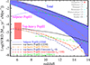 |
Fig. 13. Observed (symbols) and simulated (lines) comoving SFRDs for Salpeter (this work) and top-heavy (previous works) PopIII IMFs and model variations including: CDM and WDM (Maio & Viel 2015, 2023), non-Gaussianities (fNL = 0, 100; Maio & Iannuzzi 2011), and primordial bulk flows at 60 km/s (Maio et al. 2011b). Total SFRDs for different models and resolutions (blue shade) and JWST PopIII determinations (red shade) are also shown. Observational SFRDs are from Reddy et al. (2008), Merlin et al. (2019), Bhatawdekar et al. (2019), Bouwens et al. (2021), Donnan et al. (2023a,b), Harikane et al. (2024), and Fujimoto et al. (2025). |
Fig. 14 summarises the behaviour of the PopIII SFRD for additional models in the literature. The heterogeneity of theoretical results suggests that current uncertainties or degeneracies are still remarkable, almost two dex (z ≃ 6) or larger (z > 6), and a definitive consensus must still be reached.
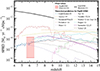 |
Fig. 14. Top-heavy PopIII SFRDs (broken lines) from simulations (Maio et al. 2010, 2011a, Pallottini et al. 2014, Xu et al. 2016, Jaacks et al. 2019, Liu & Bromm 2020, Skinner & Wise 2020, Venditti et al. 2023) and semi-analytical models (Visbal et al. 2020, Muñoz et al. 2022, Hegde & Furlanetto 2023, Sarmento & Scannapieco 2025) compared to total SFRD data (solid line) and JWST PopIII determinations (shaded area) taken from Fujimoto et al. (2025). |
4.3. Comparison with the literature
Drawing precise conclusions based on direct comparisons with observations at the epochs of interest here is not trivial and quantification of early gas phases is still an open problem. Observational determinations of stellar masses are difficult (one-dex error), as well as HI mass estimates, while H2 values rely on indirect (CO) low-z calibrations. Detections of kiloparsec-scale [CII] emission up to z ≃ 7 are consistent with the existence of significant amounts of cold gas in primordial sources (Bischetti et al. 2024; Zanella et al. 2024; Decarli & Díaz-Santos 2025; Algera et al. 2025; Narita et al. 2026; Vizgan et al. 2026; Chiang 2026), in line with our conclusions. There seems to be growing evidence of z > 6 cold outflows detected via OH+ 290 μm and OH 119 μm absorption lines tracing atomic diffuse gas and dense molecular gas, respectively (e.g. ALMA detections by Shao et al. 2022, Salak et al. 2024, and Spilker et al. 2025).
Qualitatively speaking, given the remarkable differences we find between the trends of the cosmic Ω parameters and the Ωbound ones, one must conclude that estimates of the baryon budget based on the mass of bound structures could be biased and recent ΩHI results by Oyarzún et al. (2025) go in this direction.
In large numerical simulations, H2 fractions estimated at post-processing seem to be almost insensitive to the sub-grid models adopted; however, in such analysis the cold and molecular phases cannot be directly traced due to the poor ISM physics (Ward et al. 2022, and references therein). H2 can be further explored through semi-analytical prescriptions calibrated with the present-day observed galaxy populations (Lagos et al. 2015, 2020; Diemer et al. 2018; Davé et al. 2019; Jin et al. 2021; Szakacs et al. 2022), but this approach tends to underestimate higher-z molecular masses by a factor of a few.
During the cosmic stellar-mass build-up, the amount of the mass returned to the gas phases evolves non-linearly, since the formation of stars is accompanied by a stellar return fraction, R, that grows with stellar age (Fig. 8). Although consistent with IMF and stellar-mass uncertainties (Table 3), dependences of R on stellar metallicity (Appendix A) are less severe than what is derived from analytic calculations assuming fixed metallicities (Calura et al. 2014; Vincenzo et al. 2016). More detailed analyses based on simulations that include stellar evolution, time-dependent metal spreading, and feedback mechanisms (such as the one we perform here) are still lacking in the literature.
Baryon mass functions at different z show a variety of trends with typically decreasing high-mass tails. This is somehow reminiscent of the Schechter formalism, but with more complex behaviour at the low-mass end. When comparing our results to observations of the HI mass function at z ≃ 0 by Jones et al. (2018), we see that low-z determinations are smoother and extend towards higher HI masses. This highlights a clear redshift evolution of gas mass distributions.
Baryon phases in bound objects are linked to the main galaxy properties, such as mass, SFR, and metallicity, while dependencies of our results on the specific SFR are usually weak, consistently with recent theoretical findings about early fine-structure line emission (Bisbas et al. 2022; Casavecchia et al. 2024, 2025; Muñoz-Elgueta et al. 2024; Nyhagen et al. 2025; Nakazato et al. 2026). In general, cold, warm, and hot gas masses increase with hosting Mstar, SFR, and gas Z and the found relations bare a scatter of one or two dex, as a consequence of star formation stochasticity (Katz et al. 1996). Thus, tight observational correlations might be sample-biased and capture only the trends of more powerful sources, mostly at high redshift.
The broad scatter in the gas phases is reflected in the depletion times. Observational determinations for star-forming galaxies at z ∼ 0 suggest gas depletion times of ∼2–8 Gyr (Tumlinson et al. 2017) decreasing within Mstar ∼ 108.5–1011.5 M⊙. First surveys of molecular gas in PHIBSS cosmic-noon star-forming galaxies (Tacconi et al. 2013, 2018) found tdepl, H2 ∝ (1 + z)−0.6, well approximated by tdyn ≃ tH/10. Recent estimates inferred by QSO and main-sequence galaxy observations at z ≃ 6 − 7 suggest tdepl, H2 ∼ 0.01–0.1 Gyr (Zavala et al. 2022; Salvestrini et al. 2025), in line with our results. We find that depletion times depend on redshift, but, when averaged over the z ≳ 5 range, median tdepl, H2 values are weakly dependent on gas metallicity and lie around 100 Myr as a result of turbulent (Sabbi et al. 2022), feedback-regulated star formation. Such short H2 timescales make the formation of Milky Way progenitors possible at z ≳ 6 (Rusta et al. 2024). Corresponding SFEs are around 0.01–0.04 and do not evolve significantly. In this respect, recent findings in isolated-galaxy simulations by Polzin et al. (2024) are in line with ours.
Overall, the theoretical timescales we find in primordial epochs help us understand the first phases of cosmic star formation and the role of feedback and environment in shaping the early baryon cycle. Furthermore, the impact of star formation heating explains why absorption-selected galaxies (e.g. Bollo et al. 2026) are often inefficient at converting cold gas into stars, despite their sizeable molecular reservoir.
4.4. Observational insights
From an observational point of view, measurements of MH2 and Mstar can be inferred from millimetre and optical observations, while MHI is becoming available at cosmological distances thanks to 21 cm detections. For this reason, the following definitions of observational HI and H2 gas-to-star mass fractions and baryon mass fraction are commonly adopted: μHI = MHI/Mstar, μH2 = MH2/Mstar and Fgas = MH2/(MH2 + Mstar) = μH2/(μH2 + 1).
Fig. 15 displays the evolution of the average μHI, μH2, and Fgas in the first gigayear. HI gas-to-star fractions decrease monotonically from μHI ∼ 103 at z ≳ 20 down to unity at z ≃ 5, while corresponding μH2 values range from a few to 0.1. These trends are due to the tiny amounts of stars formed in early epochs in comparison to the dominant cold-gas mass. Subsequent stellar-mass growth and the associated feedback mechanisms cause a shallower evolution of cold-gas phases and a regular decrease in both μHI and μH2. The Fgas behaviour is analogous to μH2 with values ranging between ∼0.1 (z ≃ 5) and 1 (z ≃ 20).
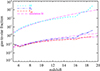 |
Fig. 15. Average μHI = MHI/Mstar (short-dashed line), μH2 = MH2/Mstar (dot-dot-dot-dashed line), and Fgas = μH2/(μH2 + 1) (dot-dashed line) redshift evolution with simulation fits (long-dashed lines; Appendix F). |
In Fig. 16 we present the dependencies of μHI, μH2, and Fgas with Mstar and corresponding fitting relations for the whole simulated data sample (Table F.2). Observational fractions decrease with Mstar. In particular, the relation between μHI and Mstar is fitted by μHI = 106.08(Mstar/M⊙)−0.76, and the resulting normalisation and slope are roughly constant in z. HI measurements from ALFALFA, GASS, COLDGASS, and xGASS data (Brown et al. 2015; Saintonge et al. 2016; Catinella et al. 2018; Guo et al. 2021) show similar slopes, of between −0.85 and −0.90. However, optically dark sources with a low surface brightness are also detected in HI and lie off the relation at Mstar ≲ 107 M⊙ (see recent WALLABY results by O’Beirne et al. 2025).
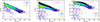 |
Fig. 16. Gas-to-star fractions, μHI (left), μH2 (centre), and Fgas = μH2/(1 + μH2) (right) as functions of Mstar compared to z ≃ 0 observational fits (dotted lines) for main-sequence galaxies (Saintonge et al. 2016, 2017; Tacconi et al. 2018). Different dotted lines in the left panel correspond to fixed Log(SFR/M⊙ yr−1) = 0, –1, –2, –3, –4, and –5, from top to bottom. Dashed magenta lines refer to simulation fits (Appendix F, Table F.2). |
Our expectations for μH2 feature a slope ranging between −0.3 (at z ≃ 16) and −0.7 (at z ≃ 5) and give μH2 ∝ Mstar−0.49 as average scaling. That broadly agrees with low-z observational results from, for example, xCOLDGASS field galaxies (Saintonge et al. 2017), EDGE-CALIFA spiral galaxies (Bolatto et al. 2017), SDSS star-forming galaxies (Popesso et al. 2020), GASP jellyfish galaxies (Moretti et al. 2023), and PHIBBS, ASPECS, and ALMA/NOEMA galaxies and cosmic-noon AGNs (Bertola et al. 2024) that similarly span a range of a few dex and feature a decreasing μH2. The exact slope of the μH2–Mstar relation is still debated. For example, the analysis by Tacconi et al. (2018) is compatible with a slope of −0.33 at z ∼ 0, while Bertola et al. (2024) find a slope of −1 at cosmic noon, without strong differences between AGN hosts and non-active galaxies. It is unclear whether this is due to possible redshift effects; however, Papastergis et al. (2012) and Peeples et al. (2014) find trends analogous to ours, with z ∼ 0 gas-to-star ratios in the range 0.1–100 and a slope between −0.48 and −0.43 using measurements by McGaugh (2005, 2012), Leroy et al. (2008) and Saintonge et al. (2011).
Our predictions for Fgas suggest typical values of between 0.1 and 0.8 for most of the sampled stellar masses and a drop below 10% at more massive scales. The trend has an average slope of roughly −0.3; however, it is better fitted by the μH2-based relation Fgas = [1 + 0.0036 (Mstar/M⊙)0.49]−1. In the figure, scattered data points below μHI, μH2, and Fgas trends represent galaxies that are either inactive or that have suffered outflow-driven HI and H2 mass removal. The Fgas bending reflects environment or feedback-induced molecular suppression and might be at the origin of the SFR-Mstar bending at later time (Popesso et al. 2019; Pérez-Martínez et al. 2025). Estimates for nearby resolved galaxies observed with Hershel agree with typical Fgas ≃ 0.04 and range between 0.02 and 0.6 depending on metallicity and dust content (Casasola et al. 2022). NOEMA determinations of z < 1 H2-cooling bright central galaxies yield Fgas ≃ 0.1–0.5 (Castignani et al. 2025). At z ≃ 1–5, observations of star-forming gas have been reporting routinely Fgas ≃ 0.3–0.8 (Daddi et al. 2010; Saintonge et al. 2011; Harris et al. 2012; Magnelli et al. 2012; Tacconi et al. 2013; Bothwell et al. 2013; Scoville et al. 2016) and studies of resolved molecular gas in z ≃ 2–3 lensed active galaxies suggest Fgas ≃ 0.6 (Spingola et al. 2020). Recent analysis of ALMA/SDSS z ≃ 2 quasars (Molyneux et al. 2025) agree with Fgas ≃ 0.02–0.24 (μH2 ≃ 0.02–0.32). Values from z ∼ 4–8 primordial galaxies show Fgas ≃ 0.3–0.9 (Dessauges-Zavadsky et al. 2020; Heintz et al. 2023; Aravena et al. 2024; Fudamoto et al. 2025). At higher z there is no convergence, yet, and upper limits at z ≃ 14 range between 0.5 (Helton et al. 2025b) and 0.8 (Schouws et al. 2025b; Carniani et al. 2025).
All these observational results together with the expected large theoretical scatter are in line with the idea that high-z star-forming galaxies might be more gas-rich than present-day ones due to their more limited evolution. Environment or dynamical conditions (mass, SFR, Z, mergers) do play a relevant role and induce significant variations in the actual abundances (as observationally suggested at lower z by e.g. Kanekar et al. 2018; Donevski et al. 2020; Zanella et al. 2023, 2026); hence, HI and H2 do not necessarily fill up the whole galaxy gas budget. The warm component can account for more than 50% of the gas content in bound structures and HI and H2 mean fractions can reach values as low as 0.2 and 10−3, respectively (Appendix D). Hints about the role of warm cosmic gas are also suggested by low-z H Lyα studies (Viel et al. 2017; Scarlata et al. 2025; Gelli et al. 2025; Rowland et al. 2025) and partially ionised atomic species, such as OVI or CIV (Peeples et al. 2014; Werk et al. 2019; Lochhaas et al. 2025). Also MgII, NII, and OIII lines are diagnostics of mildly warm gas and have been recently detected at high z (Hennawi et al. 2021; Kolupuri et al. 2025; Perna et al. 2025; Belladitta et al. 2025; Nakazato et al. 2026), but a reliable quantification has proven to be difficult. For hot gas, the situation is much more uncertain, as T > 107 K gas is mostly detected in low-z galaxy groups and clusters via X-ray emission. While hot-gas fractions can be related to total mass in both simulations and observations at z < 1 (Comparat et al. 2023; Zhang et al. 2024a,b; Rasia et al. 2025; Marini et al. 2025; Biffi et al. 2025), the high-z regime still deserves investigations. In addition, the spread among available observations is ∼dex, due to the different data (XMM-Newton, Chandra, SZ, gravitational lensing), selections (X-ray or optical), or assumptions (hydrostatic equilibrium, scaling relations) adopted to retrieve the hot mass.
5. Conclusions
In this work we have exploited the up-to-date COLDSIM numerical simulations to make predictions about the baryon budget of early galaxies and explore correlations that may be used to infer unknown quantities. We implemented detailed non-equilibrium chemistry of several chemical species, which guaranteed that HI and H2 abundances were traced consistently with metal-dependent cooling, heating, and feedback processes during cosmic structure evolution. This allowed us to explicitly follow the cold, warm, and hot gas thermal phases without relying on poorly constrained sub-grid assumptions. Our findings can be summarised as follows.
-
Baryon mass density parameters at z > 5 are dominated by gas, both in bound structures (galaxies/CGM) and in the IGM, and bound objects contain only a small fraction of the entire baryonic mass, around 10−6–10−2.
-
The cold phase dominates the epoch of reionisation, but warm gas is present by z ∼ 20 and increases with time, taking over the cosmic baryon budget at z ≲ 6.
-
Due to uncertainties in the adopted IMF, the stellar-mass density parameter can vary within 0.3 dex.
-
Phase mass functions evolve with z and show feedback-driven trends at low masses and a more regular Schechter-like shape at the high-mass end.
-
Gas phases correlate with the host galaxy Mstar and SFR, and feature a more scattered behaviour with gas Z.
-
HI traces the whole cold phase fairly well, while H2 gas is tightly linked to star formation with tdepl, H2 ∼ 0.01–0.1 Gyr.
-
Typical tdepl, HI and tdepl, H2 decrease with Mstar and SFR and correlate weakly with Z.
-
Median star formation efficiencies are around a few percent and do not evolve significantly with redshift.
-
The stellar return fraction increases up to R≃0.2 for tage ≃ 1 Gyr (a factor of two lower than the values commonly adopted) and this impacts high-z SFRDs.
-
Observation-based μHI, μH2, and Fgas fractions show decreasing trends with cosmic time, Mstar, and SFR, but cannot be considered as fair proxies of the whole galaxy gas content.
-
Matter phases and depletion times are related to host galaxy properties via simple scaling relations (see the appendix).
Acknowledgments
We thank the anonymous referee for constructive comments that allowed us to improve the original manuscript. We are grateful to V. Bollo and T. O’Beirne for useful discussions and for kindly sharing MUSE-ALMA Haloes data and to S. Fujimoto and R. P. Naidu for granting leave to reproduce their PopIII data collection. UM expresses gratitude to the Italian National Institute of Astrophysics for financial support provided through Theory Grant no. 1.05.23.06.13 “FIRST – First Galaxies in the Cosmic Dawn and the Epoch of Reionisation with High Resolution Numerical Simulations” and Travel Grant no. 1.05.23.04.01. UM also acknowledges warm hospitality at the European Southern Observatory during the completion of this work and motivating interactions with Camilla Maio. We finally acknowledge the NASA Astrophysics Data System and the JSTOR archive for their bibliographic tools.
References
- Abel, T., Anninos, P., Zhang, Y., & Norman, M. L. 1997, New Astron., 2, 181 [NASA ADS] [CrossRef] [Google Scholar]
- Abel, T., Bryan, G. L., & Norman, M. L. 2002, Science, 295, 93 [CrossRef] [Google Scholar]
- Acharya, A., Ma, Q.-B., Giri, S. K., et al. 2025, MNRAS [Google Scholar]
- Algera, H. S. B., Herrera-Camus, R., Aravena, M., et al. 2025, A&A, submitted [arXiv:2512.02320] [Google Scholar]
- Aravena, M., Heintz, K., Dessauges-Zavadsky, M., et al. 2024, A&A, 682, A24 [NASA ADS] [CrossRef] [EDP Sciences] [Google Scholar]
- Bacchini, C., Fraternali, F., Iorio, G., & Pezzulli, G. 2019, A&A, 622, A64 [NASA ADS] [CrossRef] [EDP Sciences] [Google Scholar]
- Bacchini, C., Nipoti, C., Iorio, G., et al. 2024, A&A, 687, A115 [NASA ADS] [CrossRef] [EDP Sciences] [Google Scholar]
- Bañados, E., Khusanova, Y., Decarli, R., et al. 2024, ApJ, 977, L46 [Google Scholar]
- Barberi Squarotti, M., Camera, S., & Maartens, R. 2024, JCAP, 2024, 043 [Google Scholar]
- Becker, G. D., Bolton, J. S., & Lidz, A. 2015, PASA, 32, e045 [NASA ADS] [CrossRef] [Google Scholar]
- Becker, G. D., Bolton, J. S., Zhu, Y., & Hashemi, S. 2024, MNRAS, 533, 1525 [Google Scholar]
- Behroozi, P., Wechsler, R. H., Hearin, A. P., & Conroy, C. 2019, MNRAS, 488, 3143 [NASA ADS] [CrossRef] [Google Scholar]
- Bell, E. F., & de Jong, R. S. 2001, ApJ, 550, 212 [Google Scholar]
- Bell, E. F., McIntosh, D. H., Katz, N., & Weinberg, M. D. 2003, ApJS, 149, 289 [Google Scholar]
- Belladitta, S., Bañados, E., Xie, Z.-L., et al. 2025, A&A, 699, A335 [NASA ADS] [CrossRef] [EDP Sciences] [Google Scholar]
- Bertola, E., Circosta, C., Ginolfi, M., et al. 2024, A&A, 691, A178 [NASA ADS] [CrossRef] [EDP Sciences] [Google Scholar]
- Bhatawdekar, R., Conselice, C. J., Margalef-Bentabol, B., & Duncan, K. 2019, MNRAS, 486, 3805 [NASA ADS] [CrossRef] [Google Scholar]
- Bianchetti, A., Sinigaglia, F., Rodighiero, G., et al. 2025, ApJ, 982, 82 [Google Scholar]
- Biffi, V., Rasia, E., Borgani, S., et al. 2025, A&A, 698, A238 [NASA ADS] [CrossRef] [EDP Sciences] [Google Scholar]
- Bisbas, T. G., Walch, S., Naab, T., et al. 2022, ApJ, 934, 115 [NASA ADS] [CrossRef] [Google Scholar]
- Bischetti, M., Choi, H., Fiore, F., et al. 2024, ApJ, 970, 9 [NASA ADS] [CrossRef] [Google Scholar]
- Blackwell, A. E., Bregman, J. N., & Davis, S. C. 2026, ApJ, 997, 109 [Google Scholar]
- Bolatto, A. D., Wong, T., Utomo, D., et al. 2017, ApJ, 846, 159 [Google Scholar]
- Bollo, V., Peroux, C., Zwaan, M., et al. 2026, A&A, 707, A81 [NASA ADS] [CrossRef] [EDP Sciences] [Google Scholar]
- Boogaard, L. A., Decarli, R., Walter, F., et al. 2023, ApJ, 945, 111 [NASA ADS] [CrossRef] [Google Scholar]
- Bosman, S. E. I., Fan, X., Jiang, L., et al. 2018, MNRAS, 479, 1055 [Google Scholar]
- Bothwell, M. S., Aguirre, J. E., Chapman, S. C., et al. 2013, ApJ, 779, 67 [NASA ADS] [CrossRef] [Google Scholar]
- Bouwens, R. J., Oesch, P. A., Stefanon, M., et al. 2021, AJ, 162, 47 [NASA ADS] [CrossRef] [Google Scholar]
- Bromm, V. 2013, Rep. Prog. Phys., 76, 112901 [NASA ADS] [CrossRef] [Google Scholar]
- Bromm, V., Ferrara, A., Coppi, P. S., & Larson, R. B. 2001a, MNRAS, 328, 969 [NASA ADS] [CrossRef] [Google Scholar]
- Bromm, V., Kudritzki, R. P., & Loeb, A. 2001b, ApJ, 552, 464 [NASA ADS] [CrossRef] [Google Scholar]
- Brown, T., Catinella, B., Cortese, L., et al. 2015, MNRAS, 452, 2479 [Google Scholar]
- Calura, F., Ciotti, L., & Nipoti, C. 2014, MNRAS, 440, 3341 [NASA ADS] [CrossRef] [Google Scholar]
- Cappellaro, E., Botticella, M. T., Pignata, G., et al. 2015, A&A, 584, A62 [NASA ADS] [CrossRef] [EDP Sciences] [Google Scholar]
- Carniani, S., Hainline, K., D’Eugenio, F., et al. 2024, Nature, 633, 318 [CrossRef] [Google Scholar]
- Carniani, S., D’Eugenio, F., Ji, X., et al. 2025, A&A, 696, A87 [NASA ADS] [CrossRef] [EDP Sciences] [Google Scholar]
- Casasola, V., Bianchi, S., Magrini, L., et al. 2022, A&A, 668, A130 [NASA ADS] [CrossRef] [EDP Sciences] [Google Scholar]
- Casavecchia, B., Maio, U., Péroux, C., & Ciardi, B. 2024, A&A, 689, A106 [NASA ADS] [CrossRef] [EDP Sciences] [Google Scholar]
- Casavecchia, B., Maio, U., Péroux, C., & Ciardi, B. 2025, A&A, 693, A119 [NASA ADS] [CrossRef] [EDP Sciences] [Google Scholar]
- Castignani, G., Combes, F., Salomé, P., Edge, A., & Jablonka, P. 2025, A&A, 700, A197 [NASA ADS] [CrossRef] [EDP Sciences] [Google Scholar]
- Catinella, B., Saintonge, A., Janowiecki, S., et al. 2018, MNRAS, 476, 875 [NASA ADS] [CrossRef] [Google Scholar]
- Ceverino, D., Glover, S. C. O., & Klessen, R. S. 2017, MNRAS, 470, 2791 [NASA ADS] [CrossRef] [Google Scholar]
- Chabrier, G. 2003, PASP, 115, 763 [Google Scholar]
- Chemerynska, I., Atek, H., Furtak, L. J., et al. 2024, MNRAS, 531, 2615 [NASA ADS] [CrossRef] [Google Scholar]
- Chiaki, G., Schneider, R., Nozawa, T., et al. 2014, MNRAS, 439, 3121 [NASA ADS] [CrossRef] [Google Scholar]
- Chiang, Y. K. 2026, ArXiv e-prints [arXiv:2602.02658] [Google Scholar]
- Chon, S., Ono, H., Omukai, K., & Schneider, R. 2022, MNRAS, 514, 4639 [NASA ADS] [CrossRef] [Google Scholar]
- Chon, S., Hosokawa, T., Omukai, K., & Schneider, R. 2024, MNRAS, 530, 2453 [NASA ADS] [CrossRef] [Google Scholar]
- Chowdhury, A., Kanekar, N., & Chengalur, J. N. 2022, ApJ, 941, L6 [NASA ADS] [CrossRef] [Google Scholar]
- Cicone, C., Maiolino, R., Sturm, E., et al. 2014, A&A, 562, A21 [NASA ADS] [CrossRef] [EDP Sciences] [Google Scholar]
- Cicone, C., Mainieri, V., Circosta, C., et al. 2021, A&A, 654, L8 [NASA ADS] [CrossRef] [EDP Sciences] [Google Scholar]
- Clark, P. C., Glover, S. C. O., Klessen, R. S., & Bromm, V. 2011, ApJ, 727, 110 [NASA ADS] [CrossRef] [Google Scholar]
- Comparat, J., Luo, W., Merloni, A., et al. 2023, A&A, 673, A122 [NASA ADS] [CrossRef] [EDP Sciences] [Google Scholar]
- Conselice, C. J., Adams, N., Harvey, T., et al. 2025, ApJ, 983, 30 [Google Scholar]
- Creasey, P., Theuns, T., Bower, R. G., & Lacey, C. G. 2011, MNRAS, 415, 3706 [Google Scholar]
- Croton, D. J., Springel, V., White, S. D. M., et al. 2006, MNRAS, 365, 11 [Google Scholar]
- Daddi, E., Bournaud, F., Walter, F., et al. 2010, ApJ, 713, 686 [NASA ADS] [CrossRef] [Google Scholar]
- Davé, R., Anglés-Alcázar, D., Narayanan, D., et al. 2019, MNRAS, 486, 2827 [Google Scholar]
- Davies, F. B., Bosman, S. E. I., D’Odorico, V., et al. 2026, MNRAS, 545, staf1862 [Google Scholar]
- Decarli, R., & Díaz-Santos, T. 2025, A&ARv, 33, 4 [Google Scholar]
- Decarli, R., Aravena, M., Boogaard, L., et al. 2020, ApJ, 902, 110 [Google Scholar]
- Deepak, S., Howk, J. C., Lehner, N., & Péroux, C. 2025, ApJ, 987, 199 [Google Scholar]
- D’Eramo, F., Lenoci, A., & Dekker, A. 2025, Phys. Rev. D, 112, 116008 [Google Scholar]
- Despali, G., Moscardini, L., Nelson, D., et al. 2025, A&A, 697, A213 [NASA ADS] [CrossRef] [EDP Sciences] [Google Scholar]
- Dessauges-Zavadsky, M., Ginolfi, M., Pozzi, F., et al. 2020, A&A, 643, A5 [NASA ADS] [CrossRef] [EDP Sciences] [Google Scholar]
- Dev, A., Driver, S. P., Meyer, M., et al. 2024, MNRAS, 535, 2357 [Google Scholar]
- Diemer, B., Stevens, A. R. H., Forbes, J. C., et al. 2018, ApJS, 238, 33 [NASA ADS] [CrossRef] [Google Scholar]
- Dolag, K., Borgani, S., Murante, G., & Springel, V. 2009, MNRAS, 399, 497 [Google Scholar]
- Donevski, D., Lapi, A., Małek, K., et al. 2020, A&A, 644, A144 [NASA ADS] [CrossRef] [EDP Sciences] [Google Scholar]
- Donnan, C. T., McLeod, D. J., Dunlop, J. S., et al. 2023a, MNRAS, 518, 6011 [Google Scholar]
- Donnan, C. T., McLeod, D. J., McLure, R. J., et al. 2023b, MNRAS, 520, 4554 [NASA ADS] [CrossRef] [Google Scholar]
- Donnan, C. T., Dunlop, J. S., McLure, R. J., McLeod, D. J., & Cullen, F. 2025, MNRAS, 539, 2409 [Google Scholar]
- D’Souza, R., & Bell, E. F. 2022, MNRAS, 512, 739 [CrossRef] [Google Scholar]
- Fudamoto, Y., Inoue, A. K., Bouwens, R., et al. 2025, ApJ, submitted [arXiv:2504.03831] [Google Scholar]
- Fujimoto, S., Naidu, R. P., Chisholm, J., et al. 2025, ApJ, 989, 46 [Google Scholar]
- Gallazzi, A., Brinchmann, J., Charlot, S., & White, S. D. M. 2008, MNRAS, 383, 1439 [Google Scholar]
- Galli, D., & Palla, F. 1998, A&A, 335, 403 [NASA ADS] [Google Scholar]
- Gandolfi, G., Rodighiero, G., Castellano, M., et al. 2025, A&A, 706, A364 [Google Scholar]
- Gelli, V., Mason, C., Pallottini, A., et al. 2025, A&A, submitted [arXiv:2510.01315] [Google Scholar]
- Gjergo, E., Zhang, Z., & Kroupa, P. 2026, Res. Astron. Astrophys., in press [arXiv:2601.20998] [Google Scholar]
- Gnedin, N., & Zhu, H. 2025, Open J. Astrophys., 8, 111 [Google Scholar]
- Greggio, L. 2005, A&A, 441, 1055 [NASA ADS] [CrossRef] [EDP Sciences] [Google Scholar]
- Greif, T. H., Springel, V., White, S. D. M., et al. 2011, ApJ, 737, 75 [NASA ADS] [CrossRef] [Google Scholar]
- Guo, H., Jones, M. G., Wang, J., & Lin, L. 2021, ApJ, 918, 53 [NASA ADS] [CrossRef] [Google Scholar]
- Harikane, Y., Nakajima, K., Ouchi, M., et al. 2024, ApJ, 960, 56 [NASA ADS] [CrossRef] [Google Scholar]
- Harris, A. I., Baker, A. J., Frayer, D. T., et al. 2012, ApJ, 752, 152 [NASA ADS] [CrossRef] [Google Scholar]
- Hassan, J. B., Perna, R., Cantiello, M., et al. 2025, ApJ, 992, 68 [Google Scholar]
- Hegde, S., & Furlanetto, S. R. 2023, MNRAS, 525, 428 [Google Scholar]
- Heintz, K. E., Oesch, P. A., Aravena, M., et al. 2022, ApJ, 934, L27 [NASA ADS] [CrossRef] [Google Scholar]
- Heintz, K. E., Giménez-Arteaga, C., Fujimoto, S., et al. 2023, ApJ, 944, L30 [NASA ADS] [CrossRef] [Google Scholar]
- Helton, J. M., Alberts, S., Rieke, G. H., et al. 2025a, ApJ, submitted [arXiv:2506.02099] [Google Scholar]
- Helton, J. M., Rieke, G. H., Alberts, S., et al. 2025b, Nat. Astron., 9, 729 [Google Scholar]
- Hennawi, J. F., Davies, F. B., Wang, F., & Oñorbe, J. 2021, MNRAS, 506, 2963 [NASA ADS] [CrossRef] [Google Scholar]
- Herrera-Camus, R., González-López, J., Förster Schreiber, N., et al. 2025, A&A, 699, A80 [NASA ADS] [CrossRef] [EDP Sciences] [Google Scholar]
- Herrmann, K. A., Hunter, D. A., Zhang, H.-X., & Elmegreen, B. G. 2016, AJ, 152, 177 [NASA ADS] [CrossRef] [Google Scholar]
- Hirano, S., Hosokawa, T., Yoshida, N., et al. 2014, ApJ, 781, 60 [NASA ADS] [CrossRef] [Google Scholar]
- Hollenbach, D., & McKee, C. F. 1979, ApJS, 41, 555 [Google Scholar]
- Huertas-Company, M., Shuntov, M., Dong, Y., et al. 2025, A&A, 704, A94 [NASA ADS] [CrossRef] [EDP Sciences] [Google Scholar]
- Huyan, J., Kulkarni, V. P., Poudel, S., et al. 2025, ApJ, 991, 228 [Google Scholar]
- Iben, I., Jr, & Tutukov, A. V. 1994, ApJ, 431, 264 [NASA ADS] [CrossRef] [Google Scholar]
- Jaacks, J., Finkelstein, S. L., & Bromm, V. 2019, MNRAS, 488, 2202 [NASA ADS] [CrossRef] [Google Scholar]
- Jeon, M., Pawlik, A. H., Bromm, V., & Milosavljević, M. 2014, MNRAS, 444, 3288 [Google Scholar]
- Jiang, J., Fabian, A. C., Dauser, T., et al. 2019, MNRAS, 489, 3436 [NASA ADS] [CrossRef] [Google Scholar]
- Jin, S., Dannerbauer, H., Emonts, B., et al. 2021, A&A, 652, A11 [NASA ADS] [CrossRef] [EDP Sciences] [Google Scholar]
- Jones, M. G., Haynes, M. P., Giovanelli, R., & Moorman, C. 2018, MNRAS, 477, 2 [Google Scholar]
- Kanekar, N., Prochaska, J. X., Christensen, L., et al. 2018, ApJ, 856, L23 [NASA ADS] [CrossRef] [Google Scholar]
- Kashino, D., Silverman, J. D., Rodighiero, G., et al. 2013, ApJ, 777, L8 [Google Scholar]
- Katz, N., Weinberg, D. H., & Hernquist, L. 1996, ApJS, 105, 19 [NASA ADS] [CrossRef] [Google Scholar]
- Kaur, B., Kanekar, N., Neeleman, M., et al. 2025, ApJ, 982, L26 [Google Scholar]
- Klessen, R. S., & Glover, S. C. O. 2023, ARA&A, 61, 65 [NASA ADS] [CrossRef] [Google Scholar]
- Kolupuri, S., Decarli, R., Neri, R., et al. 2025, A&A, 695, A201 [NASA ADS] [CrossRef] [EDP Sciences] [Google Scholar]
- Koribalski, B. S., Crocker, R. M., Khabibullin, I., et al. 2025, PASA, in press [arXiv:2512.15991] [Google Scholar]
- Kroupa, P. 2001, MNRAS, 322, 231 [NASA ADS] [CrossRef] [Google Scholar]
- Kulkarni, G., Keating, L. C., Haehnelt, M. G., et al. 2019, MNRAS, 485, L24 [Google Scholar]
- Kulkarni, V. P., Bowen, D. V., Straka, L. A., et al. 2022, ApJ, 929, 150 [Google Scholar]
- Lagos, C. d. P., Crain, R. A., Schaye, J., et al. 2015, MNRAS, 452, 3815 [NASA ADS] [CrossRef] [Google Scholar]
- Lagos, C. d. P., da Cunha, E., Robotham, A. S. G., et al. 2020, MNRAS, 499, 1948 [CrossRef] [Google Scholar]
- Lamperti, I., Pereira-Santaella, M., Perna, M., et al. 2022, A&A, 668, A45 [NASA ADS] [CrossRef] [EDP Sciences] [Google Scholar]
- Langan, I., Popping, G., Ginolfi, M., et al. 2026, A&A, 705, A209 [NASA ADS] [CrossRef] [EDP Sciences] [Google Scholar]
- Larson, R. B. 1998, MNRAS, 301, 569 [NASA ADS] [CrossRef] [Google Scholar]
- Leroy, A. K., Walter, F., Brinks, E., et al. 2008, AJ, 136, 2782 [Google Scholar]
- Liu, B., & Bromm, V. 2020, MNRAS, 497, 2839 [NASA ADS] [CrossRef] [Google Scholar]
- Lochhaas, C., Peeples, M. S., O’Shea, B. W., et al. 2025, ApJ, in press [arXiv:2510.25844] [Google Scholar]
- Ma, Q., Maio, U., Ciardi, B., & Salvaterra, R. 2017, MNRAS, 466, 1140 [NASA ADS] [CrossRef] [Google Scholar]
- Machida, M. N., Hirano, S., & Basu, S. 2025, ApJ, 988, 6 [Google Scholar]
- Madau, P., & Dickinson, M. 2014, ARA&A, 52, 415 [Google Scholar]
- Maeder, A. 1992, A&A, 264, 105 [NASA ADS] [Google Scholar]
- Magnelli, B., Saintonge, A., Lutz, D., et al. 2012, A&A, 548, A22 [NASA ADS] [CrossRef] [EDP Sciences] [Google Scholar]
- Maio, U., & Iannuzzi, F. 2011, MNRAS, 415, 3021 [NASA ADS] [CrossRef] [Google Scholar]
- Maio, U., & Viel, M. 2015, MNRAS, 446, 2760 [NASA ADS] [CrossRef] [Google Scholar]
- Maio, U., & Viel, M. 2023, A&A, 672, A71 [NASA ADS] [CrossRef] [EDP Sciences] [Google Scholar]
- Maio, U., Dolag, K., Ciardi, B., & Tornatore, L. 2007, MNRAS, 379, 963 [NASA ADS] [CrossRef] [Google Scholar]
- Maio, U., Ciardi, B., Dolag, K., Tornatore, L., & Khochfar, S. 2010, MNRAS, 407, 1003 [CrossRef] [Google Scholar]
- Maio, U., Khochfar, S., Johnson, J. L., & Ciardi, B. 2011a, MNRAS, 414, 1145 [NASA ADS] [CrossRef] [Google Scholar]
- Maio, U., Koopmans, L. V. E., & Ciardi, B. 2011b, MNRAS, 412, L40 [NASA ADS] [CrossRef] [Google Scholar]
- Maio, U., Salvaterra, R., Moscardini, L., & Ciardi, B. 2012, MNRAS, 426, 2078 [NASA ADS] [CrossRef] [Google Scholar]
- Maio, U., Petkova, M., De Lucia, G., & Borgani, S. 2016, MNRAS, 460, 3733 [NASA ADS] [CrossRef] [Google Scholar]
- Maio, U., Borgani, S., Ciardi, B., & Petkova, M. 2019, PASA, 36 [Google Scholar]
- Maio, U., Péroux, C., & Ciardi, B. 2022, A&A, 657, A47 [NASA ADS] [CrossRef] [EDP Sciences] [Google Scholar]
- Malloy, M., & Lidz, A. 2015, ApJ, 799, 179 [NASA ADS] [CrossRef] [Google Scholar]
- Maoz, D., & Graur, O. 2017, ApJ, 848, 25 [Google Scholar]
- Marini, I., Popesso, P., Dolag, K., et al. 2025, A&A, 698, A191 [NASA ADS] [CrossRef] [EDP Sciences] [Google Scholar]
- McGaugh, S. S. 2005, ApJ, 632, 859 [Google Scholar]
- McGaugh, S. S. 2012, AJ, 143, 40 [Google Scholar]
- Merlin, E., Fortuni, F., Torelli, M., et al. 2019, MNRAS, 490, 3309 [CrossRef] [Google Scholar]
- Messias, H., Guerrero, A., Nagar, N., et al. 2024, MNRAS, 533, 3937 [Google Scholar]
- Molyneux, S. J., Banerji, M., Temple, M. J., et al. 2025, MNRAS, 540, 1163 [Google Scholar]
- Moretti, A., Serra, P., Bacchini, C., et al. 2023, ApJ, 955, 153 [NASA ADS] [CrossRef] [Google Scholar]
- Moster, B. P., Somerville, R. S., Maulbetsch, C., et al. 2010, ApJ, 710, 903 [Google Scholar]
- Muñoz, J. B., Qin, Y., Mesinger, A., et al. 2022, MNRAS, 511, 3657 [CrossRef] [Google Scholar]
- Muñoz-Elgueta, N., Arrigoni Battaia, F., Kauffmann, G., et al. 2024, A&A, 690, A392 [NASA ADS] [CrossRef] [EDP Sciences] [Google Scholar]
- Nagamine, K., Springel, V., & Hernquist, L. 2004, MNRAS, 348, 421 [NASA ADS] [CrossRef] [Google Scholar]
- Naidu, R. P., Oesch, P. A., Brammer, G., et al. 2026, Open J. Astrophys., 9, 56033 [Google Scholar]
- Nakazato, Y., Sugimura, K., Inoue, A. K., & Ricotti, M. 2026, ApJ, 998, 26 [Google Scholar]
- Narita, K., Hatsukade, B., Fujimoto, S., et al. 2026, ApJ, 998, 42 [Google Scholar]
- Nasir, F., & D’Aloisio, A. 2020, MNRAS, 494, 3080 [Google Scholar]
- Nelson, D., Sharma, P., Pillepich, A., et al. 2020, MNRAS, 498, 2391 [NASA ADS] [CrossRef] [Google Scholar]
- Ni, Y., Li, H., Vogelsberger, M., et al. 2025, A&A, 699, A282 [NASA ADS] [CrossRef] [EDP Sciences] [Google Scholar]
- Nyhagen, C. T., Schimek, A., Cicone, C., Decataldo, D., & Shen, S. 2025, A&A, 702, A260 [NASA ADS] [CrossRef] [EDP Sciences] [Google Scholar]
- O’Beirne, T., Kilborn, V. A., Cluver, M. E., et al. 2025, MNRAS, 544, 1799 [Google Scholar]
- Omukai, K., Tsuribe, T., Schneider, R., & Ferrara, A. 2005, ApJ, 626, 627 [NASA ADS] [CrossRef] [Google Scholar]
- Oyarzún, G. A., Rafelski, M., Christensen, L., et al. 2025, ApJ, 983, 10 [Google Scholar]
- Padmanabhan, H., & Kulkarni, G. 2017, MNRAS, 470, 340 [Google Scholar]
- Palla, F., Salpeter, E. E., & Stahler, S. W. 1983, ApJ, 271, 632 [NASA ADS] [CrossRef] [Google Scholar]
- Pallottini, A., Ferrara, A., Gallerani, S., Salvadori, S., & D’Odorico, V. 2014, MNRAS, 440, 2498 [NASA ADS] [CrossRef] [Google Scholar]
- Papastergis, E., Cattaneo, A., Huang, S., Giovanelli, R., & Haynes, M. P. 2012, ApJ, 759, 138 [NASA ADS] [CrossRef] [Google Scholar]
- Parente, M., Bischetti, M., Maio, U., et al. 2026, A&A, 705, A39 [NASA ADS] [CrossRef] [EDP Sciences] [Google Scholar]
- Peeples, M. S., Werk, J. K., Tumlinson, J., et al. 2014, ApJ, 786, 54 [NASA ADS] [CrossRef] [Google Scholar]
- Pérez-Martínez, J. M., Dannerbauer, H., Emonts, B. H. C., et al. 2025, A&A, 696, A236 [NASA ADS] [CrossRef] [EDP Sciences] [Google Scholar]
- Perna, M., Arribas, S., Ji, X., et al. 2025, A&A, 694, A170 [NASA ADS] [CrossRef] [EDP Sciences] [Google Scholar]
- Péroux, C., & Howk, J. C. 2020, ARA&A, 58, 363 [CrossRef] [Google Scholar]
- Peroux, C., & Nelson, D. 2024, ArXiv e-prints [arXiv:2411.07988] [Google Scholar]
- Péroux, C., Storrie-Lombardi, L. J., McMahon, R. G., Irwin, M., & Hook, I. M. 2001, AJ, 121, 1799 [CrossRef] [Google Scholar]
- Perrotta, S., Coil, A. L., Rupke, D. S. N., et al. 2024, ApJ, 975, 263 [Google Scholar]
- Pillepich, A., Reiprich, T. H., Porciani, C., Borm, K., & Merloni, A. 2018, MNRAS, 481, 613 [Google Scholar]
- Planck Collaboration VI. 2020, A&A, 641, A6 [NASA ADS] [CrossRef] [EDP Sciences] [Google Scholar]
- Polzin, A., Kravtsov, A. V., Semenov, V. A., & Gnedin, N. Y. 2024, Open J. Astrophys., 7, 114 [Google Scholar]
- Popesso, P., Concas, A., Morselli, L., et al. 2019, MNRAS, 483, 3213 [Google Scholar]
- Popesso, P., Concas, A., Morselli, L., et al. 2020, MNRAS, 496, 2531 [NASA ADS] [CrossRef] [Google Scholar]
- Popesso, P., Concas, A., Cresci, G., et al. 2023, MNRAS, 519, 1526 [Google Scholar]
- Rao, S. M., & Turnshek, D. A. 2000, ApJS, 130, 1 [NASA ADS] [CrossRef] [Google Scholar]
- Rasia, E., Tripodi, R., Borgani, S., et al. 2025, A&A, 702, A182 [NASA ADS] [CrossRef] [EDP Sciences] [Google Scholar]
- Reddy, N. A., Steidel, C. C., Pettini, M., et al. 2008, ApJS, 175, 48 [CrossRef] [Google Scholar]
- Rodighiero, G., Cimatti, A., Gruppioni, C., et al. 2010, A&A, 518, L25 [NASA ADS] [CrossRef] [EDP Sciences] [Google Scholar]
- Rodighiero, G., Renzini, A., Daddi, E., et al. 2014, MNRAS, 443, 19 [Google Scholar]
- Romeo, A. B. 2020, MNRAS, 491, 4843 [NASA ADS] [CrossRef] [Google Scholar]
- Romeo, A. B., Agertz, O., & Renaud, F. 2020, MNRAS, 499, 5656 [NASA ADS] [CrossRef] [Google Scholar]
- Rosdahl, J., Katz, H., Blaizot, J., et al. 2018, MNRAS, 479, 994 [NASA ADS] [Google Scholar]
- Rowland, L. E., Heintz, K. E., Algera, H., et al. 2025, A&A, submitted [arXiv:2510.11351] [Google Scholar]
- Rusta, E., Salvadori, S., Gelli, V., Koutsouridou, I., & Marconi, A. 2024, ApJ, 974, L35 [Google Scholar]
- Sabbi, E., Zeidler, P., Marel, R. P. v. d., et al. 2022, ApJ, 936, 135 [Google Scholar]
- Saintonge, A., Kauffmann, G., Kramer, C., et al. 2011, MNRAS, 415, 32 [NASA ADS] [CrossRef] [Google Scholar]
- Saintonge, A., Catinella, B., Cortese, L., et al. 2016, MNRAS, 462, 1749 [Google Scholar]
- Saintonge, A., Catinella, B., Tacconi, L. J., et al. 2017, ApJS, 233, 22 [Google Scholar]
- Salak, D., Hashimoto, T., Inoue, A. K., et al. 2024, ApJ, 962, 1 [NASA ADS] [CrossRef] [Google Scholar]
- Salpeter, E. E. 1955, ApJ, 121, 161 [Google Scholar]
- Salvestrini, F., Bianchi, S., & Corbelli, E. 2025, A&A, 699, A346 [NASA ADS] [CrossRef] [EDP Sciences] [Google Scholar]
- Santini, P., Fontana, A., Castellano, M., et al. 2017, ApJ, 847, 76 [NASA ADS] [CrossRef] [Google Scholar]
- Santoro, F., & Shull, J. M. 2006, ApJ, 643, 26 [NASA ADS] [CrossRef] [Google Scholar]
- Sargent, M. T., Daddi, E., Béthermin, M., et al. 2014, ApJ, 793, 19 [NASA ADS] [CrossRef] [Google Scholar]
- Sarmento, R., & Scannapieco, E. 2025, ApJ, 988, 221 [Google Scholar]
- Saslaw, W. C., & Zipoy, D. 1967, Nature, 216, 976 [NASA ADS] [CrossRef] [Google Scholar]
- Scarlata, C. M., Hu, W., Hayes, M. J., et al. 2025, ApJ, 985, 115 [Google Scholar]
- Schady, P., Yates, R. M., Christensen, L., et al. 2024, MNRAS, 529, 2807 [NASA ADS] [CrossRef] [Google Scholar]
- Schouws, S., Bouwens, R. J., Algera, H., et al. 2025a, ApJ, submitted [arXiv:2502.01610] [Google Scholar]
- Schouws, S., Bouwens, R. J., Ormerod, K., et al. 2025b, ApJ, 988, 19 [Google Scholar]
- Schreiber, C., Pannella, M., Elbaz, D., et al. 2015, A&A, 575, A74 [NASA ADS] [CrossRef] [EDP Sciences] [Google Scholar]
- Scoville, N., Sheth, K., Aussel, H., et al. 2016, ApJ, 820, 83 [Google Scholar]
- Shao, Y., Wang, R., Weiss, A., et al. 2022, A&A, 668, A121 [NASA ADS] [CrossRef] [EDP Sciences] [Google Scholar]
- Silk, J. 1983, MNRAS, 205, 705 [Google Scholar]
- Skinner, D., & Wise, J. H. 2020, MNRAS, 492, 4386 [NASA ADS] [CrossRef] [Google Scholar]
- Speagle, J. S., Steinhardt, C. L., Capak, P. L., & Silverman, J. D. 2014, ApJS, 214, 15 [Google Scholar]
- Spilker, J. S., Champagne, J. B., Fan, X., et al. 2025, ApJ, 982, 72 [Google Scholar]
- Spina, B., Bosman, S. E. I., Davies, F. B., Gaikwad, P., & Zhu, Y. 2024, A&A, 688, L26 [NASA ADS] [CrossRef] [EDP Sciences] [Google Scholar]
- Spingola, C., McKean, J. P., Vegetti, S., et al. 2020, MNRAS, 495, 2387 [Google Scholar]
- Springel, V. 2005, MNRAS, 364, 1105 [Google Scholar]
- Stacy, A., McKee, C. F., Lee, A. T., Klein, R. I., & Li, P. S. 2022, MNRAS, 511, 5042 [NASA ADS] [CrossRef] [Google Scholar]
- Stefanon, M., Bouwens, R. J., Labbé, I., et al. 2021, ApJ, 922, 29 [NASA ADS] [CrossRef] [Google Scholar]
- Storrie-Lombardi, L. J., & Wolfe, A. M. 2000, ApJ, 543, 552 [Google Scholar]
- Szakacs, R., Péroux, C., Zwaan, M. A., et al. 2022, MNRAS, 512, 4736 [NASA ADS] [CrossRef] [Google Scholar]
- Tacchella, S., Bose, S., Conroy, C., Eisenstein, D. J., & Johnson, B. D. 2018, ApJ, 868, 92 [NASA ADS] [CrossRef] [Google Scholar]
- Tacconi, L. J., Neri, R., Genzel, R., et al. 2013, ApJ, 768, 74 [NASA ADS] [CrossRef] [Google Scholar]
- Tacconi, L. J., Genzel, R., Saintonge, A., et al. 2018, ApJ, 853, 179 [Google Scholar]
- Tacconi, L. J., Genzel, R., & Sternberg, A. 2020, ARA&A, 58, 157 [NASA ADS] [CrossRef] [Google Scholar]
- Tornatore, L., Ferrara, A., & Schneider, R. 2007, MNRAS, 382, 945 [NASA ADS] [CrossRef] [Google Scholar]
- Tumlinson, J., Peeples, M. S., & Werk, J. K. 2017, ARA&A, 55, 389 [Google Scholar]
- Vanzella, E., Messa, M., Zanella, A., et al. 2026, A&A, 705, L12 [NASA ADS] [CrossRef] [EDP Sciences] [Google Scholar]
- Venditti, A., Graziani, L., Schneider, R., et al. 2023, MNRAS, 522, 3809 [NASA ADS] [CrossRef] [Google Scholar]
- Viel, M., Haehnelt, M. G., Bolton, J. S., et al. 2017, MNRAS, 467, L86 [NASA ADS] [CrossRef] [Google Scholar]
- Villaescusa-Navarro, F., Anglés-Alcázar, D., Genel, S., et al. 2021, ApJ, 915, 71 [NASA ADS] [CrossRef] [Google Scholar]
- Vincenzo, F., Matteucci, F., Belfiore, F., & Maiolino, R. 2016, MNRAS, 455, 4183 [Google Scholar]
- Visbal, E., Bryan, G. L., & Haiman, Z. 2020, ApJ, 897, 95 [NASA ADS] [CrossRef] [Google Scholar]
- Vizgan, D., Vieira, J. D., Spilker, J. S., et al. 2026, ApJ, in press [arXiv:2601.04133] [Google Scholar]
- Walter, F., Carilli, C., Neeleman, M., et al. 2020, ApJ, 902, 111 [Google Scholar]
- Ward, S. R., Harrison, C. M., Costa, T., & Mainieri, V. 2022, MNRAS, 514, 2936 [NASA ADS] [CrossRef] [Google Scholar]
- Weng, S., Sadler, E. M., Foster, C., et al. 2022, MNRAS, 512, 3638 [NASA ADS] [CrossRef] [Google Scholar]
- Werk, J. K., Rubin, K. H. R., Bish, H. V., et al. 2019, ApJ, 887, 89 [NASA ADS] [CrossRef] [Google Scholar]
- Whelan, J., & Iben, I., Jr 1973, ApJ, 186, 1007 [Google Scholar]
- Wise, J. H., Turk, M. J., Norman, M. L., & Abel, T. 2012, ApJ, 745, 50 [NASA ADS] [CrossRef] [Google Scholar]
- Wolfe, A. M., Lanzetta, K. M., Foltz, C. B., & Chaffee, F. H. 1995, ApJ, 454, 698 [Google Scholar]
- Xu, H., Norman, M. L., O’Shea, B. W., & Wise, J. H. 2016, ApJ, 823, 140 [NASA ADS] [CrossRef] [Google Scholar]
- Yoshida, N., Omukai, K., & Hernquist, L. 2007, ApJ, 667, L117 [NASA ADS] [CrossRef] [Google Scholar]
- Zanchettin, M. V., Ramos Almeida, C., Audibert, A., et al. 2025, A&A, 695, A185 [NASA ADS] [CrossRef] [EDP Sciences] [Google Scholar]
- Zanella, A., Valentino, F., Gallazzi, A., et al. 2023, MNRAS, 524, 923 [CrossRef] [Google Scholar]
- Zanella, A., Iani, E., Dessauges-Zavadsky, M., et al. 2024, A&A, 685, A80 [NASA ADS] [CrossRef] [EDP Sciences] [Google Scholar]
- Zanella, A., Belli, S., Valentino, F. M., & Bolamperti, A. 2026, A&A, in press https://doi.org/10.1051/0004-6361/202558073 [Google Scholar]
- Zang, S.-H., & Zhu, H.-M. 2024, ApJ, 961, 160 [Google Scholar]
- Zavala, J. A., Casey, C. M., Scoville, N., et al. 2019, ApJ, 887, 183 [NASA ADS] [CrossRef] [Google Scholar]
- Zavala, J. A., Casey, C. M., Spilker, J., et al. 2022, ApJ, 933, 242 [CrossRef] [Google Scholar]
- Zhang, Y., Comparat, J., Ponti, G., et al. 2024a, A&A, 690, A267 [NASA ADS] [CrossRef] [EDP Sciences] [Google Scholar]
- Zhang, Y., Comparat, J., Ponti, G., et al. 2024b, A&A, 690, A268 [NASA ADS] [CrossRef] [EDP Sciences] [Google Scholar]
- Zhu, H., Avestruz, C., & Gnedin, N. Y. 2020, ApJ, 899, 137 [Google Scholar]
- Zhu, Y., Becker, G. D., Bosman, S. E. I., et al. 2024, MNRAS, 533, L49 [NASA ADS] [CrossRef] [Google Scholar]
Appendix A: Numerical effects
In Fig. A.1 the impact of different box resolutions and sizes on the evolution of the matter density parameters is shown for cold, warm, hot and stellar phases in the Ref, HR, and LB runs. Results converge to the same behaviour in all the boxes.
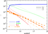 |
Fig. A.1. Redshift evolution of the mass density parameters for the cold (solid lines), warm (dotted lines), hot (dashed lines) and stellar (dot-dashed lines) components in the Ref (thick lines), HR (regular lines) and LB (thin lines) simulations. |
Figs. A.2 and A.3 show the resulting distributions for the stellar return fraction R at z ≃ 6, and its evolution as function of redshift and stellar age, as described by the fitting expression of eq. 2: R(tage) = 0.0885 Log(tage/3.853Myr). R values are obtained from self-consistent stellar-evolution calculations including time-dependent metal enrichment for a Salpeter IMF.
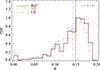 |
Fig. A.2. Probability distributions (histograms) and median values (vertical lines) of R for the Ref (solid black lines), HR (dashed orange lines) and LB (dot-dot-dot-dashed purple lines) simulations at z ≃ 6. |
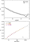 |
Fig. A.3. Top: Redshift evolution of the average R at different redshifts for the Ref (solid black lines), HR (dashed orange lines) and LB (dot-dot-dot-dashed purple lines) simulations. Bottom: Dependence of R on stellar age at z ≃ 2 (crosses), 6 (diamonds) and 18 (triangles), plotted together with the fitting function of eq. 2 (solid line). |
Further numerical effects are discussed about stellar-metallicity dependences of the stellar return fraction R in Fig. A.4. We find metallicity-driven variations from a few up to some ten percent with stronger impacts at high redshift, as demonstrated by the R distributions for metallicity-selected structures (Z < 0.001 Z⊙ and Z > 0.1 Z⊙). At z ≃ 6, 9 and 12, sample peak and median are both around R ≃ 0.15, 0.11 and 0.09. Metal-poor populations, that are older and more evolved, feature corresponding values of R ∼ 0.17, 0.12 and 0.09, while younger metal-rich populations have R ∼ 0.14, 0.09 and 0.06.
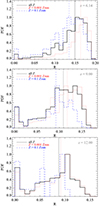 |
Fig. A.4. Probability distribution functions (histograms) and median values (vertical lines) of R computed for the Ref run at redshift z ≃ 6, 9 and 12 for different stellar metallicities: all Z (solid black lines), Z < 0.001 Z⊙ (dotted red lines) and Z > 0.1 Z⊙ (dashed blue lines). |
Appendix B: Selection effects
In Fig. B.1, we show halo mass functions obtained with different selection criteria. Total-mass functions and virial-mass functions feature similar trends, with slight differences in the low-mass tail. When haloes with more than 300 member particles are considered, the low-mass tail is statistically less populated as tiny objects, presumably not well resolved, are excluded.
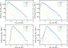 |
Fig. B.1. Top row: Halo total-mass functions (left) and virial-mass functions (right) at z = 5.25, 6.14, 8.09, 10.00, 13.01, 16.00. Bottom row: Corresponding functions for haloes with more than 300 particles. |
In Fig. B.2 we show the impacts of selection effects in terms of the relative contribution to the total mass locked in bound objects when different mass or number thresholds are applied.
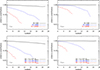 |
Fig. B.2. Top row: Contribution to the total gas mass (left) and stellar mass (right) of haloes with a number of particles N > 100 (solid lines), 1 000 (dot-dashed lines), 10 000 (dashed lines) as a function of redshift. Bottom row: Contribution of haloes with total mass M > 5 × 10⁷ (solid lines), 109 (dot-dashed lines) and 1010 M⊙ (dashed lines). |
Appendix C: Main sequence
With the selection performed in this work (more than 300 particles to resolve the virial mass of haloes), we retrieve the basic relations involving SFR, stellar mass and halo mass at different epochs, as plotted in Fig. C.1. The simulated main sequence at different z (upper panel) can be fitted by eq. 1 with the values of the parameters a and b listed in Table F.1. The values we find are in good agreement with z ≃ 5 observational determinations (Rodighiero et al. 2010, 2014; Kashino et al. 2013; Speagle et al. 2014; Schreiber et al. 2015; Popesso et al. 2023; Herrera-Camus et al. 2025). The simulated relation between stellar mass and halo mass (lower panel) features a generally increasing trend at all z. Recent literature works adopting heterogeneous numerical techniques are in line with the broad scatter we find at low masses (Ceverino et al. 2017; Rosdahl et al. 2018; Tacchella et al. 2018; Behroozi et al. 2019; Zhu et al. 2020; Romeo et al. 2020; Stefanon et al. 2021).
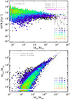 |
Fig. C.1. Top: Simulated sSFR and Mstar at different z (coloured symbols), z ≃ 5 observational fits by Speagle et al. (2014), Santini et al. (2017) and Popesso et al. (2023) (thin, regular and thick dotted lines) and z ∼ 0.5 MUSE-ALMA determinations (circles) with upper limits (arrows) by Bollo et al. (2026). Fits to simulation data at each z (thin dashed lines) are displayed together with the fit to the whole simulated sample (thick dashed magenta line), as per eq. 1 and Table F.1: Log10(SFR/Gyr−1) = 1.871 − 0.187 Log10(Mstar/M⊙). Bottom: Simulated Mstar and Mvir and fits from a low-z semi-analytical model (Croton et al. 2006, SAM, thick dotted line) and the stellar-to-halo mass relation (Moster et al. 2010, SHMR, thin dotted line). |
Appendix D: Mass fractions and phases
In the top panel of Fig. D.1 the ratios between the bound-object mass density parameters and the cosmic mass density parameters are shown for each baryon phase. Similarly, results for the IGM-to-cosmic ratios are shown in the bottom panel. At early times, most of the cosmic gas is in the cold (HI) phase, but, due to the rarity of primordial objects, cold bound gas accounts for only Ωbound, cold/Ωcold ≲ 10−4 (z ≃ 18). The amount of warm cosmic gas is tiny in comparison to cold cosmic gas (Fig. 2) and is typically bound (Ωbound, warm/Ωwarm > 50% at z ≃ 18). While cosmic evolution proceeds, more and more gas experiences cooling, star formation and feedback effects in growing galaxies. These processes boost Ωbound, H2/ΩH2 up to ∼0.8, lower ΩIGM, H2/ΩH2 down to ∼0.2 and lead to Ωbound, hot/Ωhot ∼ 0.1–1% at z ≃ 6–10.
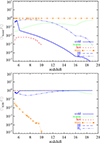 |
Fig. D.1. Bound-to-cosmic (top) and IGM-to-cosmic (bottom) mass density ratio for the cold, warm, hot, stellar, HI and H2 baryon phases. |
In Fig. D.2, we display the mean redshift evolution of the bound-object mass fractions for the cold, warm, hot, stellar, HI and H2 baryon phase, computed as < fphase > =Mphase/Mgas = Ωbound, phase/(Ωbound, cold+Ωbound, warm+Ωbound, hot), where, Mphase and Mgas are the total bound masses in the considered phase and in the gas, respectively. Clearly, the cold and warm phases dominate the halo mass content at z ≳ 6 and z ≲ 6, respectively, and the cold and warm fractions lie around 0.3 and 0.7 at z ≃ 5. Hot gas is always subdominant, with average fractions that increase from ∼10−6 at z ≃ 10 to about 5 × 10⁻³ at z ≃ 5, while star fractions follow star formation activity increasing from ∼10−4 at z ≃ 19 to 0.1 at z ≃ 5. HI and H2 phases feature trends that are almost flat with average H2-to-HI ratios ∼0.001-0.05.
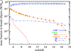 |
Fig. D.2. Average mass fraction of each baryon phase (cold, warm, hot, stars, HI, H2) identified in bound objects at different redshifts. |
Cold, warm and hot simulated gas fractions at different z as functions of virial mass, stellar mass, SFR and gas Z are displayed in Fig. D.3, while the trends for HI and H2 gas fractions are presented in Fig. D.4. These quantities are theoretically consistent, but they are hard to be proven observationally, since detecting all the gaseous components and estimating the total gas mass in galaxies is challenging. So, in Fig. D.5, we normalise the HI and H2 fractions by accounting for the cold component only, i.e.: fHI, cold = MHI/Mcold and fH2, cold = MH2/Mcold. These quantities are closer to observations when HI and/or H2 can be considered good tracers of the gas budget (e.g. Bacchini et al. 2019, 2024). The figures show fHI, cold ≃ 0.75 for all the galaxy populations sampled at different z, while fH2, cold reaches values up to ∼0.2–0.3, i.e. some dex higher than fH2. These results are consequences of the fact that HI is only present in the cold phase, where most H2 is formed. In general, H2 molecules are susceptible to non-equilibrium, environment and feedback effects, as highlighted by the scatter in both fH2 (Fig. D.4) and fH2, cold (Fig. D.5). These results are consistent with Figs. 6 and 7.
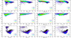 |
Fig. D.3. Cold (top row), warm (central row) and hot (bottom row) gas fraction versus virial mass (first column), stellar mass (second column), SFR (third column) and gas metallicity (fourth column) at z = 5.25, 6.14, 8.09, 10.00, 13.01, and 16.01. |
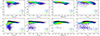 |
Fig. D.4. HI (top) and H2 (bottom) mass fractions versus virial mass, stellar mass, SFR and gas metallicity, respectively from left to right, at z = 5.25, 6.14, 8.09, 10.00, 13.01, and 16.01. |
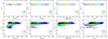 |
Fig. D.5. HI (top) and H2 (bottom) cold-mass fractions versus virial mass, stellar mass, SFR and gas metallicity, respectively from left to right, at z = 5.25, 6.14, 8.09, 10.00, 13.01, and 16.01. |
Appendix E: Depletion times
HI and H2 gas depletion times as function of stellar mass Mstar, gas metallicity Z and sSFR can be found in Fig. E.1. Data points show rather broad relations due to the role of feedback and environment in shaping gas properties at all times. The values of tdepl, HI and tdepl, H2 decrease with stellar mass and metallicity and minimum values are reached in star-forming structures with Mstar ∼ 108–109 M⊙ and Z > 0.01 Z⊙. The similarity of these trends with the ones with SFR in Fig. 10 is simply understood in terms of the main-sequence and mass-metallicity relations.
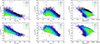 |
Fig. E.1. H2 (top) and HI (bottom) depletion times versus stellar mass (left), gas metallicity (centre) and sSFR (right) at z = 5.25, 6.14, 8.09, 10.00, 13.01, and 16.01. Simulation fits (dashed magenta lines) are in Appendix F. |
Appendix F: Fitting functions
We fit simulated results in the base-10 logarithmic form

where x and y are dimensionless, non-negative variables and a and b are fit parameters.
We consider data for masses, SFR and metallicities both at individual redshifts and in the whole z > 5 range (all z). Masses and metallicities are expressed in solar units, SFR in M⊙ yr−1, depletion times in Gyr and sSFR in Gyr−1.
In Table F.1 we report a and b parameters for the main sequence and the relations between Mcold, Mwarm, Mhot vs Mstar or SFR:
Fit parameters for the main sequence (sSFR vs. Mstar) and the relations between Mcold or Mwarm or Mhot and Mstar or SFR. Mass is in solar units, SFR in solar masses per year and sSFR in Gyr−1.
Log(sSFR/Gyr−1) = a + b Log(Mstar/M⊙)
Log(Mcold/M⊙) = a + b Log(Mstar/M⊙)
Log(Mwarm/M⊙) = a + b Log(Mstar/M⊙)
Log(Mhot/M⊙) = a + b Log(Mstar/M⊙)
Log(Mcold/M⊙) = a + b Log[SFR/(M⊙ yr−1)]
Log(Mwarm/M⊙) = a + b Log[SFR/(M⊙ yr−1)]
Log(Mhot/M⊙) = a + b Log[SFR/(M⊙ yr−1)].
Parameter determinations for the Mhot relations are missing at z ≳ 10 due to lack of statistics. To remove resolution artefacts, we fit the data for objects with stellar masses and hot-gas masses above 2 × 10⁶ M⊙ and SFR> 3 × 10⁻² M⊙ yr−1.
In Table F.2 we quote a and b parameters for the relations between MHI or MH2 and Mvir or Mstar and for the relations between MHI or MH2 and SFR:
Fit parameters for MHI or MH2 and Mvir, Mstar and SFR relations, as well as for gas-to-star fractions μHI and μH2 versus Mstar with mass in solar units and SFR in solar masses per year.
Log(MHI/M⊙) = a + b Log(Mvir/M⊙)
Log(MH2/M⊙) = a + b Log(Mvir/M⊙)
Log(MHI/M⊙) = a + b Log(Mstar/M⊙)
Log(MH2/M⊙) = a + b Log(Mstar/M⊙)
Log(MHI/M⊙) = a + b Log[SFR/(M⊙ yr−1)]
Log(MH2/M⊙) = a + b Log[SFR/(M⊙ yr−1)].
Results for HI and H2 gas-to-star fractions μHI = MHI/Mstar and μH2 = MH2/Mstar as functions of Mstar are also fitted as:
Log μHI = a + b Log(Mstar/M⊙)
Log μH2 = a + b Log(Mstar/M⊙).
Corresponding Fgas values are obtained via Fgas = μH2/(μH2 + 1).
Fit parameters for HI and H2 depletion times, tdepl, HI and tdepl, H2, as functions of Mstar, SFR, gas Z and sSFR are quoted in Table F.3 for the expressions below:
Fit parameters for HI and H2 depletion times tdepl, HI and tdepl, H2 in Gyr versus Mstar, SFR, gas Z and sSFR with mass in solar units, SFR in solar masses per year, Z in units of Z⊙ and sSFR in Gyr−1.
Log(tdepl, HI/Gyr) = a + b Log(Mstar/M⊙)
Log(tdepl, H2/Gyr) = a + b Log(Mstar/M⊙)
Log(tdepl, HI/Gyr) = a + b Log[SFR/(M⊙ yr−1)]
Log(tdepl, H2/Gyr) = a + b Log[SFR/(M⊙ yr−1)]
Log(tdepl, HI/Gyr) = a + b Log(Z/Z⊙)
Log(tdepl, H2/Gyr) = a + b Log(Z/Z⊙)
Log(tdepl, HI/Gyr) = a + b Log(sSFR/Gyr−1)
Log(tdepl, H2/Gyr) = a + b Log(sSFR/Gyr−1).
Redshift evolution of the median tdepl, HI and tdepl, H2 is:
Log(tdepl, HI/Gyr) = 1.345 − 0.170 Log(1 + z)
Log(tdepl, H2/Gyr) = 0.943 − 2.045 Log(1 + z).
Their behaviour is bracketed by the average trends
Log(tdepl, HI/Gyr) = − 1.177 + 1.578 Log(1 + z)
Log(tdepl, H2/Gyr) = − 1.499 − 0.236 Log(1 + z)
and the mean trends
Log(tdepl, HI/Gyr) = 2.857 − 1.301 Log(1 + z)
Log(tdepl, H2/Gyr) = 2.273 − 3.065 Log(1 + z).
The evolution of the average μHI and μH2 is given by:
Log μHI = −3.379 + 4.813 Log(1 + z)
Log μH2 = −3.700 + 2.300 Log(1 + z)
with 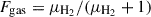 .
.
We fit the recovery timescale for 15-200 M⊙ stars as:
Log(trec/Myr) = 3.295 − 2.349Log(tage/Myr), equivalent to
Log(trec/Myr) = − 0.424 + 1.307Log(Mstar/M⊙).
The fitting function for the stellar return fraction R (eq. 2) is:

for stellar ages tage > 3.853 Myr and R = 0 otherwise.
All Tables
Fit parameters for the main sequence (sSFR vs. Mstar) and the relations between Mcold or Mwarm or Mhot and Mstar or SFR. Mass is in solar units, SFR in solar masses per year and sSFR in Gyr−1.
Fit parameters for MHI or MH2 and Mvir, Mstar and SFR relations, as well as for gas-to-star fractions μHI and μH2 versus Mstar with mass in solar units and SFR in solar masses per year.
Fit parameters for HI and H2 depletion times tdepl, HI and tdepl, H2 in Gyr versus Mstar, SFR, gas Z and sSFR with mass in solar units, SFR in solar masses per year, Z in units of Z⊙ and sSFR in Gyr−1.
All Figures
|
Fig. 1. Mass-weighted temperature maps at z ≃ 14, 10 and 6 smoothed on a grid of 1024 pixels a side for the gas in the largest halo that has a physical virial radius (circles) of ∼2.4, 5.9, and 18.7 kpc and a total mass of 1.4 × 10⁹, 7.3 × 10⁹, and 6.9 × 10¹⁰ M⊙, respectively, from left to right. |
| In the text | |
|
Fig. 2. Baryon density parameters as function of redshift for cold (solid line), warm (dotted line), hot (short-dashed line), stellar (dot-dashed line with asterisks), HI (long-dashed line), and H2 (dot-dot-dot-dashed line) phases. The horizontal grey line marks the value of Ω0, b. |
| In the text | |
|
Fig. 3. Cold (top), warm (centre), and hot (bottom) gas mass functions at z = 5.25, 6.14, 8.09, 10.00, 13.01, and 16.01. |
| In the text | |
|
Fig. 4. HI (top), H2 (centre), and stellar (bottom) mass functions at different z with a fit to z = 0 ALFALFA HI data by Jones et al. (2018) (top panel, dotted grey line), z = 6–10 HST/Spitzer masses by Stefanon et al. (2021) (bottom panel, coloured crosses) and expectations by Jaacks et al. (2019) (bottom panel, coloured diamonds). |
| In the text | |
|
Fig. 5. Baryon density parameters in bound objects (left) and the IGM (right) as function of redshift for cold (solid lines), warm (dotted lines), hot (short-dashed lines), stellar (dot-dashed lines with asterisks), HI (long-dashed lines), and H2 (dot-dot-dot-dashed lines) phases. The horizontal grey line marks the value of Ω0, b. Stars form out of cold gas that dominates the baryon budget at z ≳ 6 and is overtaken by warm gas at later times. |
| In the text | |
|
Fig. 6. Cold (left column), warm (central column), and hot (right column) gas mass versus Mstar (top row) and SFR (bottom row) for galaxies at redshift z = 5.25, 6.14, 8.09, 10.00, 13.01, and 16.01, with simulation fits (dashed magenta lines) reported in Appendix F (Table F.1). Different gas phases probe different Mstar and SFR regimes with little redshift evolution, but a large environment and feedback-driven scatter. |
| In the text | |
|
Fig. 7. HI (top) and H2 (bottom) masses versus Mvir (left), Mstar (centre), and SFR (right). Observational fits for HI and H2 data are shown by grey dotted lines and MUSE-ALMA Haloes H2 upper limits (Bollo et al. 2026) by grey circles and arrows. The fit to the MUSE-ALMA Haloes MHI vs. Mstar is Log(MHI/M⊙) = 0.50 Log(Mstar/M⊙)+4.52 (O’Beirne et al. 2026, priv. comm.) and is extrapolated from galaxy data at Mstar ∼ 108–1012 M⊙. Multi-parametric fits by Salvestrini et al. (2025) are shown for SFR = 10−1 M⊙ yr−1 (lower central panel) and Mstar = 108.5, 107, and 105.5 M⊙ (dotted lines from top to bottom in the lower right panel). Simulation fits (dashed magenta lines) are in Appendix F (Table F.2). Results are little dependent on redshift and feature a large environment-driven scatter. |
| In the text | |
|
Fig. 8. Stellar return fraction R as a function of stellar age for simulated data at redshifts z = 5 (crosses), 12 (diamonds), and 18 (triangles) in the Ref run. Data points refer to median R values with median absolute deviation, while the solid grey line is the corresponding fit (Eq. 2). |
| In the text | |
|
Fig. 9. Redshift evolution of average (regular lines), mean (thin lines), and median (thick lines) HI and H2 depletion times compared to dynamical time, tdyn (dotted black line), and observational expectations by Bollo et al. (2026) at low z (crosses with 1σ dispersion) and Péroux & Howk (2020) at z≃5–6 (diamonds with 1σ dispersion). Simulation fits (Appendix F) are overplotted with long-dashed magenta lines. |
| In the text | |
|
Fig. 10. H2 (top) and HI (bottom) depletion times versus SFR at z = 5.25, 6.14, 8.09, 10.00, 13.01, and 16.01 with simulation fits (Appendix F, Table F.3). Further trends with galaxy properties are in Appendix E. |
| In the text | |
|
Fig. 11. Median HI (thin symbols) and H2 (thick symbols) depletion times vs Z at different z (coloured symbols) and for the whole z range (solid magenta lines). Gas metallicity affects depletion times at all z. |
| In the text | |
|
Fig. 12. Top: Median SFE redshift evolution with 1σ spread (top) for all (solid line) and star-forming (short-dashed line) objects. Bottom: Median trec/tdepl, H2 ratios with 1σ spread for trec, low = 9 Myr (long-dashed line) and 3 Myr (dot-dashed line) lower limits. |
| In the text | |
|
Fig. 13. Observed (symbols) and simulated (lines) comoving SFRDs for Salpeter (this work) and top-heavy (previous works) PopIII IMFs and model variations including: CDM and WDM (Maio & Viel 2015, 2023), non-Gaussianities (fNL = 0, 100; Maio & Iannuzzi 2011), and primordial bulk flows at 60 km/s (Maio et al. 2011b). Total SFRDs for different models and resolutions (blue shade) and JWST PopIII determinations (red shade) are also shown. Observational SFRDs are from Reddy et al. (2008), Merlin et al. (2019), Bhatawdekar et al. (2019), Bouwens et al. (2021), Donnan et al. (2023a,b), Harikane et al. (2024), and Fujimoto et al. (2025). |
| In the text | |
|
Fig. 14. Top-heavy PopIII SFRDs (broken lines) from simulations (Maio et al. 2010, 2011a, Pallottini et al. 2014, Xu et al. 2016, Jaacks et al. 2019, Liu & Bromm 2020, Skinner & Wise 2020, Venditti et al. 2023) and semi-analytical models (Visbal et al. 2020, Muñoz et al. 2022, Hegde & Furlanetto 2023, Sarmento & Scannapieco 2025) compared to total SFRD data (solid line) and JWST PopIII determinations (shaded area) taken from Fujimoto et al. (2025). |
| In the text | |
|
Fig. 15. Average μHI = MHI/Mstar (short-dashed line), μH2 = MH2/Mstar (dot-dot-dot-dashed line), and Fgas = μH2/(μH2 + 1) (dot-dashed line) redshift evolution with simulation fits (long-dashed lines; Appendix F). |
| In the text | |
|
Fig. 16. Gas-to-star fractions, μHI (left), μH2 (centre), and Fgas = μH2/(1 + μH2) (right) as functions of Mstar compared to z ≃ 0 observational fits (dotted lines) for main-sequence galaxies (Saintonge et al. 2016, 2017; Tacconi et al. 2018). Different dotted lines in the left panel correspond to fixed Log(SFR/M⊙ yr−1) = 0, –1, –2, –3, –4, and –5, from top to bottom. Dashed magenta lines refer to simulation fits (Appendix F, Table F.2). |
| In the text | |
|
Fig. A.1. Redshift evolution of the mass density parameters for the cold (solid lines), warm (dotted lines), hot (dashed lines) and stellar (dot-dashed lines) components in the Ref (thick lines), HR (regular lines) and LB (thin lines) simulations. |
| In the text | |
|
Fig. A.2. Probability distributions (histograms) and median values (vertical lines) of R for the Ref (solid black lines), HR (dashed orange lines) and LB (dot-dot-dot-dashed purple lines) simulations at z ≃ 6. |
| In the text | |
|
Fig. A.3. Top: Redshift evolution of the average R at different redshifts for the Ref (solid black lines), HR (dashed orange lines) and LB (dot-dot-dot-dashed purple lines) simulations. Bottom: Dependence of R on stellar age at z ≃ 2 (crosses), 6 (diamonds) and 18 (triangles), plotted together with the fitting function of eq. 2 (solid line). |
| In the text | |
|
Fig. A.4. Probability distribution functions (histograms) and median values (vertical lines) of R computed for the Ref run at redshift z ≃ 6, 9 and 12 for different stellar metallicities: all Z (solid black lines), Z < 0.001 Z⊙ (dotted red lines) and Z > 0.1 Z⊙ (dashed blue lines). |
| In the text | |
|
Fig. B.1. Top row: Halo total-mass functions (left) and virial-mass functions (right) at z = 5.25, 6.14, 8.09, 10.00, 13.01, 16.00. Bottom row: Corresponding functions for haloes with more than 300 particles. |
| In the text | |
|
Fig. B.2. Top row: Contribution to the total gas mass (left) and stellar mass (right) of haloes with a number of particles N > 100 (solid lines), 1 000 (dot-dashed lines), 10 000 (dashed lines) as a function of redshift. Bottom row: Contribution of haloes with total mass M > 5 × 10⁷ (solid lines), 109 (dot-dashed lines) and 1010 M⊙ (dashed lines). |
| In the text | |
|
Fig. C.1. Top: Simulated sSFR and Mstar at different z (coloured symbols), z ≃ 5 observational fits by Speagle et al. (2014), Santini et al. (2017) and Popesso et al. (2023) (thin, regular and thick dotted lines) and z ∼ 0.5 MUSE-ALMA determinations (circles) with upper limits (arrows) by Bollo et al. (2026). Fits to simulation data at each z (thin dashed lines) are displayed together with the fit to the whole simulated sample (thick dashed magenta line), as per eq. 1 and Table F.1: Log10(SFR/Gyr−1) = 1.871 − 0.187 Log10(Mstar/M⊙). Bottom: Simulated Mstar and Mvir and fits from a low-z semi-analytical model (Croton et al. 2006, SAM, thick dotted line) and the stellar-to-halo mass relation (Moster et al. 2010, SHMR, thin dotted line). |
| In the text | |
|
Fig. D.1. Bound-to-cosmic (top) and IGM-to-cosmic (bottom) mass density ratio for the cold, warm, hot, stellar, HI and H2 baryon phases. |
| In the text | |
|
Fig. D.2. Average mass fraction of each baryon phase (cold, warm, hot, stars, HI, H2) identified in bound objects at different redshifts. |
| In the text | |
|
Fig. D.3. Cold (top row), warm (central row) and hot (bottom row) gas fraction versus virial mass (first column), stellar mass (second column), SFR (third column) and gas metallicity (fourth column) at z = 5.25, 6.14, 8.09, 10.00, 13.01, and 16.01. |
| In the text | |
|
Fig. D.4. HI (top) and H2 (bottom) mass fractions versus virial mass, stellar mass, SFR and gas metallicity, respectively from left to right, at z = 5.25, 6.14, 8.09, 10.00, 13.01, and 16.01. |
| In the text | |
|
Fig. D.5. HI (top) and H2 (bottom) cold-mass fractions versus virial mass, stellar mass, SFR and gas metallicity, respectively from left to right, at z = 5.25, 6.14, 8.09, 10.00, 13.01, and 16.01. |
| In the text | |
|
Fig. E.1. H2 (top) and HI (bottom) depletion times versus stellar mass (left), gas metallicity (centre) and sSFR (right) at z = 5.25, 6.14, 8.09, 10.00, 13.01, and 16.01. Simulation fits (dashed magenta lines) are in Appendix F. |
| In the text | |
Current usage metrics show cumulative count of Article Views (full-text article views including HTML views, PDF and ePub downloads, according to the available data) and Abstracts Views on Vision4Press platform.
Data correspond to usage on the plateform after 2015. The current usage metrics is available 48-96 hours after online publication and is updated daily on week days.
Initial download of the metrics may take a while.