| Issue |
A&A
Volume 708, April 2026
|
|
|---|---|---|
| Article Number | A60 | |
| Number of page(s) | 19 | |
| Section | Extragalactic astronomy | |
| DOI | https://doi.org/10.1051/0004-6361/202557667 | |
| Published online | 26 March 2026 | |
GRB 180728A and SN 2018fip: The nearest high-energy cosmological gamma-ray burst with an associated supernova
1
INAF – Osservatorio di Astrofisica e Scienza dello Spazio, Via Piero Gobetti 93/3, 40129 Bologna, Italy
2
INAF, Osservatorio Astronomico di Capodimonte, Salita Moiariello 16, 80131 Naples, Italy
3
DARK, Niels Bohr Institute, University of Copenhagen, Jagtvej 128, 2200 Copenhagen, Denmark
4
Department of Astronomy, Kyoto University, Kitashirakawa-Oiwake-cho, Sakyo-ku, Kyoto 606-8502, Japan
5
Department of Physics, University of Bath, Claverton Down, Bath BA2 7AY, UK
6
Cosmic Dawn Center (DAWN)
7
Niels Bohr Institute, University of Copenhagen, Jagtvej 128, 2200 Copenhagen N, Denmark
8
Department of Astrophysics/IMAPP, Radboud University, 6525 AJ, Nijmegen, The Netherlands
9
Hessian Research Cluster ELEMENTS, Giersch Science Center, Max-von-Laue-Stra βe 12, Goethe University Frankfurt, Campus Riedberg, D-60438 Frankfurt am Main, Germany
10
Instituto de Astrofísica de Andalucía (IAA-CSIC), Glorieta de la Astronomía s/n, 18008 Granada, Spain
11
Thüringer Landessternwarte Tautenburg, Sternwarte 5, 07778 Tautenburg, Germany
12
INAF – Osservatorio Astronomico di Brera, Via E. Bianchi 46, I-23807 Merate (LC), Italy
13
Artemis, Université de la Côte d’Azur, Observatoire de la Côte d’Azur, CNRS, 06304 Nice, France
14
Aix Marseille Univ, CNRS, LAM, Marseille, France
15
Department of Physics, Royal Holloway – University of London, Egham TW20 0EX, U.K.
16
Lomonosov Moscow State University, 119234 Moscow, Universitetskiy prospekt, 13, Moscow, Russia
17
School of Physics and Centre for Space Research, University College Dublin, Belfield D04 V1W8 Dublin, Ireland
18
INAF, Osservatorio Astronomico di Roma, Via Frascati 33, I-00078 Monte Porzio Catone (Roma), Italy
19
Department of Physics, Lancaster University, Lancs LA1 4YB, UK
20
Center for Interdisciplinary Exploration and Research in Astrophysics (CIERA), Northwestern University, 1800 Sherman Avenue, Evanston, IL 60201, USA
21
School of Physics and Astronomy, University of Leicester, University Road, Leicester LE1 7RH, UK
22
Space Science Data Center (SSDC) – Agenzia Spaziale Italiana (ASI), Via del Politecnico snc, I-00133 Roma, Italy
23
Astrophysics Research Institute, Liverpool John Moores University, 146 Brownlow Hill, Liverpool L3 5RF, UK
24
Max-Planck-Institut für Extraterrestrische Physik, Giessenbachstraße 1, 85748 Garching, Germany
25
The Oskar Klein Centre, Department of Astronomy, AlbaNova SE-106 91 Stockholm, Sweden
26
School of Mathematical and Physical Sciences, Macquarie University, NSW 2109, Australia
★ Corresponding author: This email address is being protected from spambots. You need JavaScript enabled to view it.
Received:
13
October
2025
Accepted:
16
January
2026
Abstract
Context. The long gamma-ray burst GRB 180728A at a redshift of z = 0.1171 stands out due to its high isotropic energy of Eγ, iso ≈ 2.5 × 1051 erg, in contrast with most events at redshift z < 0.2, but it is comparable to the bulk of luminous bursts more common at higher redshift.
Aims. We aim to study the properties of GRB 180728A’s prompt emission, afterglow, and associated supernova (SN 2018fip), comparing them with other GRB-SN events.
Methods. This study employs a dense photometric and spectroscopic follow-up of the afterglow and the SN up to 80 days after the burst. We used image subtraction to remove the presence of a nearby bright star, and modelled both the afterglow and the supernova.
Results. This event lies on the Ep, i–Eγ, iso plane occupied by classical collapsar events, and the prompt emission is one of the most energetic at z < 0.2 after GRB 030329 and GRB 221009A. The afterglow of GRB 180728A is less luminous than that of most long GRBs, showing a shallow early phase that steepens after about 5 hours (0.2 days). The GRB exploded in an irregular low-mass blue star-forming galaxy, which is typical of low-z collapsar events. Because of the relatively faint afterglow, the light curve bump of SN 2018fip dominates the optical emission already after approximately 3 days and is one of the best sampled to date. The strong suppression below ∼4000 Å and a largely featureless continuum in the early 6–9 day spectra favour aspherical two-component ejecta with a high-velocity collimated component (> 20 000 km s−1), that is dominant early on and a more massive low-velocity component that dominates at much later epochs.
Conclusions. Our findings indicate that asymmetries need to be considered in order to better understand GRB-SNe. In any case, SN 2018fip shares many characteristics with typical GRB-SNe. Its kinetic energy is below the common range of 1052–1053 erg and does not correlate with the high energy of the GRB, highlighting the complexity and diversity of the GRB-SN energy budget partition.
Key words: gamma-ray burst: general / supernovae: general / supernovae: individual: SN 2018fip / gamma-ray burst: individual: GRB 180728A
Deceased.
© The Authors 2026
 Open Access article, published by EDP Sciences, under the terms of the Creative Commons Attribution License (https://creativecommons.org/licenses/by/4.0), which permits unrestricted use, distribution, and reproduction in any medium, provided the original work is properly cited.
This article is published in open access under the Subscribe to Open model. This email address is being protected from spambots. You need JavaScript enabled to view it. to support open access publication.
1. Introduction
Gamma-ray bursts (GRBs) are the most energetic explosions in the Universe. They have at least two different progenitors: the collapse of fast-rotating very massive stars (collapsar model, e.g., Woosley & Bloom 2006) which leads to broad-lined Type Ic core-collapse supernovae (SNe) (Cano et al. 2017b), or the merger of compact objects including at least one neutron star, which can be observed as kilonovae (KNe; e.g., Abbott et al. 2017a,b). Although some exceptions have been found (e.g., Ahumada et al. 2021; Rossi et al. 2022b; Levan et al. 2023), collapsar events are usually responsible for long-duration GRBs (LGRBs), which have a duration longer than ∼2 s (see, e.g. Bromberg et al. 2012) and a soft energy spectrum (Mazets et al. 1981; Kouveliotou et al. 1993).
The association of LGRBs with massive stars has been established since the association of the nearby and low energy GRB 980425 with the well studied SN 1998bw, the prototypical GRB-SN (e.g., Galama et al. 1998; Woosley et al. 1999; Nakamura et al. 2001; Sollerman et al. 2002; Woosley & Bloom 2006; Clocchiatti et al. 2011; Modjaz et al. 2016). All known GRB-SNe are Type Ic with broad line features (SNe Ic-BL), explosions of highly stripped stars that lack signatures of hydrogen and helium in their spectra (e.g., Woosley & Bloom 2006; Cano et al. 2017b). Most GRB-SNe share a similar luminosity1, energy release, ejecta, and nickel masses (e.g., Cano et al. 2017b; Izzo et al. 2019; Klose et al. 2019; Melandri et al. 2022), regardless of the energy of the GRB, whether they are a low-energy2 GRB, such as GRB 060218 (e.g. Pian et al. 2006; Mazzali et al. 2006), or a highly energetic GRB, such as GRB 130427A (e.g., Xu et al. 2013; Melandri et al. 2014). The only rare exceptions are the superluminous SN 2011kl associated with the ultra-long GRB 111209A (Kann et al. 2019) and the putatively most luminous GRB-SN associated with the otherwise unexceptional GRB 140506A3 (Kann et al. 2024a).
In contrast to the GRB-SN properties, LGRBs have a wide range of emitted isotropic energy (Eγ, iso of 1048–1055 erg; e.g., Minaev & Pozanenko 2020; Tsvetkova et al. 2021). Due to selection effects (e.g., Minaev & Pozanenko 2020), most events within z < 0.2 are low-energy GRBs, with an isotropic energy of 1048–1050 erg, while high-redshift events have large gamma-ray energies, 1051–1055 erg (e.g., Minaev & Pozanenko 2020; Tsvetkova et al. 2021). Among the dozen LGRBs at z < 0.2, only two have Eγ, iso > 1050 erg, GRB 030329 at z = 0.167 (Hjorth et al. 2003; Matheson et al. 2003; Stanek et al. 2003), and the exceptional brightest of all time (BOAT) GRB 221009A (Burns et al. 2023) at z = 0.151 (Malesani et al. 2025) with its Eγ, iso ≈ 1055 erg (Frederiks et al. 2023).
Of the thousands of known LGRBs, an associated SN has been identified in only about 50 cases through late-time bumps in their optical afterglow light curves, since such signals become progressively too faint to detect at high redshifts. Moreover, there are accurate spectroscopic observations of only about 30 GRB-SNe, because only the low-redshift events can be studied in detail (e.g., Galama et al. 1998; Hjorth et al. 2003; Izzo et al. 2019; Cano et al. 2017a; Ashall et al. 2019; Melandri et al. 2019; Kann et al. 2019; Melandri et al. 2022). The SNe associated with events at redshifts beyond z = 0.2 are usually too faint for spectroscopic follow-up from the ground, except for the brightest events at z ≳ 0.3, such as GRB 130427A – SN 2013cq at z = 0.3399 (e.g., Xu et al. 2013; Melandri et al. 2014), or more recently GRB 230812B – SN 2023pel z = 0.360 (Srinivasaragavan et al. 2024a; Roman Aguilar et al. 2025), and even their photometric follow-up requires a substantial observational effort (e.g., Klose et al. 2019).
The only nearby high-energy event whose afterglow (unlike GRB 221009A) did not outshine its associated SN is GRB 030329 (Shrestha et al. 2023; Levan et al. 2023; Blanchard et al. 2024; Srinivasaragavan et al. 2023), and its proximity allows for detailed study from its rise. With just this one case, the connection between GRB energy and SN properties remains uncertain. Within the collapsar scenario, the observed burst duration is just the difference between the engine operating time and the jet breakout time (e.g., Bromberg et al. 2012). Numerical simulations have shown that the longest-lasting engines result in the most successful gamma-ray bursts (the result is also a function of the viewing angle), those in which the jet breaks out of the star’s surface (Lazzati et al. 2012, 2013). Most of the energy produced powers the SN ejecta, while only a small fraction is sufficient for the jet to penetrate the stellar envelope and produce the GRB and the afterglow (e.g., Mazzali et al. 2014; Ashall et al. 2019). However, the simple assumption of a spherical explosion is not the best model. In particular, (Ashall et al. 2019) find that the emission of SN 2016jca (GRB 161219B) is a highly aspherical explosion viewed close to the on-axis jet, due to the very early SN spectroscopic identification. (Izzo et al. 2019) reached similar conclusions in the case of SN 2017iuk (GRB 171205A).
In this paper, we present a comprehensive analysis of the optical and near-infrared (NIR) counterpart of GRB 180728A and of the associated supernova. This event has a gamma-ray energy of ≈2 × 1051 erg (Frederiks et al. 2018), firmly placing it in the high-energy population of GRBs. In Rossi et al. (2018), we reported the detection in our first afterglow spectra of absorption features at a common redshift of z = 0.117 (refined to 0.1171 in Section 3.2), which we consider to be the redshift of GRB 180728A. In Izzo et al. (2018) and Selsing et al. (2018) we reported the spectroscopic discovery of the emerging SN, named SN 2018fip in the Transient Name Server4.
In Sects. 2 and 3 of this paper, we present the available multi-band data. In Sect. 4, we present the results of our analysis of the afterglow, host galaxy, and SN spectra. In Sect. 5, we discuss our analysis, and in Sect. 6, we present our conclusions. Throughout this work, we adopt the notation according to which the flux density of a counterpart is described as Fν(t)∝t−αν−β, and we use a Lambda cold dark matter (ΛCDM) world model with ΩM = 0.308, ΩΛ = 0.692, and H0 = 67.8 km s−1 Mpc−1 (Planck Collaboration XIII 2016). The redshift of z = 0.117 thus corresponds to a luminosity distance of 562 Mpc, and at this redshift 1 arcsec corresponds to 2.2 kpc. Significant Galactic extinction affects the field (AV = 0.74 mag; Schlafly & Finkbeiner 2011). We report magnitudes in the AB system, and we report times in the observer frame, unless otherwise specified.
2. Observations
2.1. The burst
The Burst Alert Telescope (BAT; Barthelmy et al. 2005) on board the Neil GehrelsSwift Observatory satellite (Gehrels et al. 2004) detected the bright LGRB 180728A at t0 = 17:29:00 UT on the 28th of July 2018 (Starling et al. 2018). The prompt emission shows a faint precursor lasting about 3 s followed by a single but brighter pulse. This began at t0 + 11 s, peaked at t0 + 13 s, and faded to background at t0 + 40 s. The total duration of the burst measured by BAT in the 15–350 keV energy range is T90 = 8.68 ± 0.30 s (Markwardt et al. 2018). Konus-Wind (KW; Frederiks et al. 2018) and Astrosat CZTI (Sharma et al. 2018) also detected the burst, while the Gamma-Ray Burst Monitor (GBM) on board the Fermi satellite (Veres et al. 2018) detected its precursor.
2.2. Afterglow photometry
The MASTER Global Robotic Net (Lipunov et al. 2010) pointed at GRB 180728A with MASTER-SAAO, located at the South African Astronomical Observatory starting 22 s after notice time (38 s after trigger time) on 2018-07-28 17:29:38 UT (Lipunov et al. 2018a,b). In the first 10 s exposure the MASTER auto-detection system discovered the optical afterglow in both polarisation filters (see Sect. 3.1 where we provide a refined localisation). MASTER followed-up the afterglow every night until 2018-08-18 with both MASTER-OAFA (located at the Observatorio Astronomico Felix Aguilar) and SAAO (Lipunov et al. 2018c).
We conducted additional early optical and NIR observations using the 0.6-meter robotic Rapid Eye Mount (REM) telescope (Zerbi et al. 2001; Covino et al. 2004), located at the European Southern Observatory (ESO) in La Silla, Chile. Observations began on 28 July 2018, about 0.18 days after the burst event, and lasted for several hours. We performed further ground-based observations using the multichannel imager GROND (Greiner et al. 2008) mounted on the MPG 2.2 m telescope on La Silla, Chile. GROND started observing on 2018-08-01, 3.3 days after the GRB trigger. Starting 5.6 hours after the trigger, we have also used the acquisition camera of the X-shooter instrument.
Swift did not slew immediately due to an Earth limb constraint (Starling et al. 2018). The X-Ray Telescope (XRT; Burrows et al. 2005) and the UltraViolet and Optical Telescope (UVOT; Roming et al. 2005) aboard Swift began observing GRB 180728A 1730.8 s (0.02 days) after the BAT trigger (Perri et al. 2018). Swift/XRT found an unknown X-ray source with an uncertainty of 5.8 arcseconds (radius, 90% containment). A UVOT-enhanced position gave the localisation to within 1 5 radius (90% containment) and was consistent with the optical counterpart (Osborne et al. 2018). XRT observations continued for more than 2 months after the GRB, when the source became too faint to be detected. Swift/UVOT began settled observations of the field 1740 s after the BAT trigger, and initial results were reported in Laporte & Starling (2018), where they report the detection of a source consistent with the enhanced XRT position and the optical transient (OT) discovered with MASTER.
2.3. Spectroscopic follow-up
We obtained ultraviolet (UV) to NIR spectroscopic observations of the afterglow and SN with the X-shooter instrument (Vernet et al. 2011) mounted on the Very Large Telescope (VLT) on Paranal (ESO, Chile). The spectra cover a wavelength range from 3300–22 500 Å. We obtained the first three spectra under the ESO program 0101.D-0648 (PI: N. Tanvir), and the following spectra under the DDT ESO program 2101.D-5044 (PI: A. Rossi).
Starting with the fourth epoch, we placed the slit at a position angle of 118.1°, chosen to cover both the afterglow and the nearby star, as shown in Fig. 1. Note that by chance the slit covered both objects also during the first observation. Observations were obtained by nodding along the slit with an offset of 5″ between exposures in a standard ABBA sequence. We used slit widths of  ,
,  and
and  for the UVB, VIS and NIR spectrograph arms, respectively, resulting in resolving powers of R = λ/Δλ ≈ 4400, 7400 and 5400. Our spectroscopic campaign is summarised in Table 1. Selsing et al. (2018) reported that significant features in the spectrum develop and become more prominent 23 days after the GRB (21 days in the rest frame). These features resemble those of SNe Type-Ic at maximum light (see Sect. 4.5).
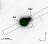 |
Fig. 1. Image of the optical afterglow of GRB 180728A obtained in the r-band with the X-shooter acquisition camera on 28 July 2018, 0.23 days after the burst trigger. We highlight the position of the afterglow (indicated as “AG”) and of the nearby star, together with their projected distance. The rectangle shows the X-shooter slit with a position angle of 118.1 deg, which we selected to cover both the afterglow and the nearby star starting with the fourth observation at 6.26 days. The green contours indicate equal count levels. |
Spectroscopic observations obtained with X-shooter.
3. Data reduction
3.1. Imaging
We extracted Swift/UVOT source counts using a region of 3″ radius. In order to be consistent with the UVOT calibration, we then corrected these count rates to 5″ using the curve of growth contained in the calibration files (Poole et al. 2008). Within this extraction region there is contamination from a relatively bright nearby star in the UVOT white, b and v filters (see Fig. 1), which we subtracted using late-time imaging. The star was too faint in the UV and not a significant source of contamination at those wavelengths. We obtained the count rates from the images using the Swift tool UVOTSOURCE and converted to magnitudes using the UVOT photometric zero points. Contamination-corrected fluxes can be found in Table C.3.
MASTER observed the OT in both polarisation filters (Pola1 and Pola2 in Table C.3) and in the Clear CR band (best described by GAIA g filter). Unfortunately, we could not measure any polarisation. The list of reference stars is in Table C.2. After astrometric calibration and combine of the images, we performed standard aperture photometry as described in Lipunov et al. (2019). In the attempt to detect the SN component, deep observations in the Clear-band were obtained after the first night. These frames were stacked and an upper limit was calculated for each of the resulting total frames.
The REM data reduction was performed using standard procedures, including image alignment, stacking, and sky subtraction. The images were automatically reduced using the jitter script of the eclipse package (Devillard 1997) which aligns and stacks the images to obtain one average image for each sequence. A combination of IRAF (Tody 1993) and SExtractor packages (Bertin & Arnouts 2010) was used to perform aperture photometry. Given the relatively low signal-to-noise ratio of the individual images, we combined multiple frames, obtaining a significant detection in the SDSS g′r′i′z′ filters at 0.25 days.
The images from X-shooter g′r′z′ and GROND g′r′i′z′JHKs were reduced in a standard manner using PyRAF/IRAF (Tody 1993). In particular, for GROND, a dedicated pipeline was used as described in Krühler et al. (2008). Astrometry was calibrated against field stars in the GAIA DR2 catalogue (Gaia Collaboration 2018), obtaining an astrometric precision of 0 17. The coordinates of the transient are RA,Dec(J2000)
  ,
,  . In GROND and X-shooter images the nearby star makes it difficult to perform photometry, especially when the OT is fainter than the star and the seeing is comparable or larger than the projected offset (Fig. 1). To remove the contamination of this star, we used image-subtraction using deep X-shooter and GROND reference images obtained more than 220 days after the GRB under clear sky conditions with seeing
  and
and  for the X-shooter and GROND, respectively. Before applying image subtraction, the input and reference images were aligned using the WCSREMAP package (Mink 1997). Image subtraction was then performed using a routine based on HOTPANTS5 (Becker 2015). To calibrate the g′r′i′z′ photometry we used secondary standards (Table C.1) in the field observed with GROND 16.3 days after trigger, and calibrated with the SDSS field STD176 observed immediately after and under photometric conditions. Calibration of the field in JHKs was performed using 2MASS stars (Skrutskie et al. 2006).
Finally, we corrected all the data for Galactic extinction using the extinction curve derived by Cardelli et al. (1989), E(B − V) = 0.238 mag from the dust maps of Schlafly & Finkbeiner (2011), and an optical total-to-selective extinction ratio RV = 3.1. In Table C.3 we report our full dataset before correction for Galactic extinction.
3.2. Spectroscopy of the optical transient
We reduced the spectra following the procedure described in Selsing et al. (2019), which includes a cosmic-ray removal algorithm (van Dokkum 2001) applied to the raw spectra, after which each individual exposure was reduced with the version v. 3.5.0 of the ESO X-shooter pipeline (Modigliani et al. 2010). The pipeline produces a flat-fielded, rectified, and wavelength-calibrated 2D spectrum for every frame in the UVB, VIS, and NIR arms. We then combined the different frames using custom-made post-processing scripts7. Background light from a nearby bright foreground star complicated the extraction of the 1D spectrum. We used an extraction region from −3 to +3 pixels (equivalent to 0.96″) to limit the contamination from the stellar source. The final extracted 1D spectra were then corrected for slit loss and Galactic extinction along the line-of-sight of the burst using the dust maps of Schlafly & Finkbeiner (2011). Wavelengths are reported in vacuum and in the barycentric frame of the Solar System. After analyzing the final reduction of the first spectra, we have refined the redshift to be z = 0.1171 ± 0.0001, determined from the detection of absorption features due to Mg II λλ2796,2803, Mg I λ2853, and Ca II λλ3934,3969, as first reported in Rossi et al. (2018).
4. Data analysis
4.1. Prompt emission phase
The prompt emission of GRB 180728A was measured and characterised by the three main GRB detectors currently in operation: Swift/BAT (Markwardt et al. 2018), Fermi/GBM (Veres et al. 2018), and Konus-WIND (Frederiks et al. 2018). The light curve of this event consists of a weak and soft ‘precursor’ followed by a bright and harder pulse (see also Hu et al. 2021), making it one of those cases in which the estimates of the observer-frame spectral peak energy Ep and, to a lesser extent, of the total radiated energy Eγ, iso depend significantly on the combination of the energy band and detector sensitivity, as well as on the exposure time over which the spectrum and fluence were measured.
In order to check the consistency of this event with the Ep, i-Eγ, iso correlation8 of LGRBs (Amati et al. 2002; Amati 2006), we adopted the conservative approach of taking into account the fluence and Ep estimates for all three instruments. In the case of BAT we performed our own analysis, following the standard data reduction and analysis recipes9. Based on the above and assuming the standard flat ΛCDM cosmology, we derived an isotropic equivalent radiated energy Eγ, iso in the 1–10 000 keV cosmological rest-frame of (2.5 ± 0.5)×1051 erg and a rest-frame, intrinsic spectral peak energy Ep, i of 123 ± 28 keV. As shown in Figure 2, these values make GRB 180728A well consistent with the Ep, i-Eγ, iso correlation (e.g., Amati et al. 2002). With the values above, GRB 180728A had an isotropic gamma-ray equivalent luminosity of log Liso [erg s−1] = 50.4 and falls in the category of high-luminosity GRBs (Hjorth 2013; Cano et al. 2017b).
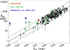 |
Fig. 2. GRB 180728A (red) in the Ep, i − Eγ, iso plane. The GRBs with an associated SN are highlighted in green; outliers are in blue. Dot-dashed lines indicate the ±2σ region. The GRB data are from Amati et al. (2019). |
4.2. Light curve analysis – The afterglow and supernova
The very early MASTER light curve shows a shallow, then steeper, rise to peak. To model this peak, we excluded the first two data points, where residual prompt emission might still be present. Therefore, we modelled data up to 0.05 days after the trigger with a rise breaking to a decay using a smoothly broken power law (Beuermann et al. 1999): F = (F1n + F2n)−1/n, where Fx = fb(t/tb)−αx10, with fb as the flux density at break time tb; n as the break smoothness parameter; and the subscripts 1, 2 indicating pre- and post-break, respectively. In particular, using the subscript r,d for the rise and decay around the early peak, we found αr = −0.66 ± 0.16, αd = 0.431 ± 0.011, and tb, peak = 0.0024 ± 0.0002 days (211 ± 16 s).
Data following the peak can also be fit with a smoothly broken power law, in addition to an SN component (the underlying host-galaxy component has been subtracted). As previously reported in Izzo et al. (2018), there is clear evidence of a ∼0.5 mag rebrightening in the X-shooter r-band between 6 and 13 days, thus indicating an emerging SN component in the optical light curve. Therefore, we fit the afterglow of GRB 180728A as well as SN 2018fip in the k, s context (Zeh et al. 2004). Here, we assume that the SN light curve evolves similarly to SN 1998bw associated with GRB 980425 (Galama et al. 1998; Patat et al. 2001; Clocchiatti et al. 2011), modified by the luminosity factor k and the stretch factor s. A value of k = 1 implies that the GRB-SN is just as luminous as SN 1998bw in the specific rest-frame band corresponding to the observer-frame band in which the measurements were taken. Furthermore, without changing its fundamental shape, the light curve’s temporal evolution can be compressed (s < 1) or stretched (s > 1) with the stretch factor, s. This is a powerful analysis method, as GRB-SNe are found to generally agree well with the light curve shape of SN 1998bw (Ferrero et al. 2006; Klose et al. 2019; Kann et al. 2024a).
We performed a joint fit of all bands except the GROND H and K bands, which have so few detections that they do not contribute to the fit. In this fit, the parameters α1, α2, tb and n are shared between all bands. Similarly, we assumed no host galaxy contribution in any band. We did not find any systematic offsets among Sloan g′r′z′ from X-shooter, GROND g′r′z′ data, and MASTER CR data. Therefore, we combined similar filters into single light curves. We note that only GROND systematically observed in i′ and the NIR filters, except for one REM epoch with g′r′i′z′ photometry at ∼0.25 days. As GROND data dominate, especially during the SN phase, we used these filters when filter-specific parameters were needed. For all bands where a SN contribution was detected (GROND g′r′i′z′J), we derived SN 1998bw model light curves in these filters at the redshift of GRB 180728A following the method detailed in Zeh et al. (2004) and Klose et al. (2019). The luminosity factor k and the stretch factor s were left free to vary individually for each band. The derived kg′…J parameters represent the exact SN 1998bw light curve for each filter. As the data density is high, we initially decided to leave the break smoothness n free to vary. However, this resulted in a degenerate fit which did not converge after over a thousand Levenberg-Marquardt least-squares iterations. Because the light curve break clearly shows a very smooth rollover, we fixed n = 1. The results are given in Table 211. The n = 1 fit is also more consistent with the expected values for a typical GRB geometry (van Eerten & MacFadyen 2013; Lamb et al. 2021). The break is achromatic, a characteristic feature of jet breaks (e.g., Rhoads 1997, 1999), which is clear in the optical bands (Fig. 3). We can therefore exclude an origin related to the passage of a spectral break (e.g., Sari et al. 1998). Alternative scenarios such as reverse shocks or a sudden energy injection would instead produce a bump or a steep-to-shallow transition in the light curve (e.g., Sari & Mészáros 2000; Zhang & Mészáros 2002; Granot et al. 2003; Nakar & Granot 2007). We therefore conclude that this feature is most likely the jet break of the afterglow. The pre- and post-break decay indices are shallower than expected for a classical jet break, and may be explained by a non-constant environment (e.g., wind) with the possible presence of continuous (rather than sudden) energy injection (e.g., Zhang et al. 2006; Racusin et al. 2009) and/or by a slightly off-axis structured jet (e.g. Ryan et al. 2020). An advanced numerical modelling goes beyond the goals of this work.
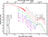 |
Fig. 3. Fit to the light curve and supernova of GRB 180728A. Magnitudes are in the AB system and corrected for Galactic foreground extinction, and time is in the observer frame. For reasons of clarity, light curves in each filter are offset by the magnitude values noted in the legend. Starting at ≈300 s, the light curve in all bands except for H and K is fitted with a broken power law plus individual SN component. The dashed line for the white filter is an extrapolation because the points at > 4 days were not fitted. See text for details. |
Afterglow and supernova fit results.
Given the very low line-of-sight extinction in the host galaxy of GRB 180728A (see Sect. 4.3), the k values derived from the fit require no further correction. We find SN 2018fip is generally somewhat fainter than SN 1998bw, 80–90% of its luminosity, except for the J band, where it is somewhat brighter (but we caution the error here is larger, and SN 1998bw itself has very sparse and late J-band data Patat et al. 2001; Sollerman et al. 2002). It also evolves a bit faster than SN 1998bw, at a stretch of 80–100%. This makes SN 2018fip a very typical GRB-SN. We also note that this SN joins the small group of GRB-SN with NIR detections, which includes SN2010bh, SN2011kl, SN2013dx, and SN1998bw. The fitted model allowed us to disentangle the afterglow and SN contributions from the data, producing high-quality ‘pure’ afterglow and SN-only data12.
4.3. The early optical to X-ray spectral energy distribution
We used Xspec v12.13.0 (Arnaud 1996) to simultaneously model the optical and X-ray spectral energy distribution (SED) at the logarithmic mean time of 0.03, 0.1, 0.24 and 1.5 days, corresponding to the first, second, and fourth Swift/XRT observing epochs, and an additional late time epoch before the rise of the SN and corresponding to the third VLT/X-shooter spectra. They correspond also to 2 epochs before and 2 epochs after the break in the light curve (at about 0.1–0.2 days, see Sect. 4.2 and Table 2). To build these SEDs, we first created the XRT spectra using the time-slice tool in the XRT repository (Evans et al. 2007, 2009). We then shifted the optical data closer to these times using the decay indices found above. For all epochs we applied a Galactic equivalent hydrogen column density of  (Willingale et al. 2013) and a foreground Galactic dust extinction (Sect. 3.1). The redshift was fixed to z = 0.117. For the last epoch at 1.5 days, we used the pure afterglow magnitudes obtained from the procedure described above (Sect. 4.2)13.
We started analyzing the data from the last 2 epochs, to avoid possible degeneracy between the fireball model breaks in the SED and the absorption. At late times the breaks are commonly far from the optical and XRT bands, and after the jet break they should not shift in time, according to the standard fireball scenario. These late-time fits show that a single power law fits both epochs well (Fig. 4). Therefore, it is reasonable to assume that these two epochs share the same physical synchrotron emission model. We jointly fit both epochs with the same shared parameters and we find the best fit ( ) for a common spectral slope of
  , with intrinsic
  and negligible intrinsic dust extinction. This is in particular best modelled with E(B − V) = 0.012 ± 0.009 mag and the Large Magellanic Cloud (LMC) extinction law (Pei 1992), compared to Small Magellanic Cloud (SMC) or Milky Way (MW) laws, which also explains the possible 2175 Å absorption feature visible in the uvm2-band in the earliest SEDs (see Appendix B and Fig. B.1).
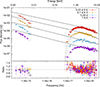 |
Fig. 4. X-ray to optical SED at 0.03, 0.1, 0.24 and 1.5 days. The last two epochs are well modelled by a joint-fit with a single power law with spectral slope β ∼ 0.7. In the first two epochs, the optical data have a slightly shallower spectral slope, βopt ∼ 0.6, while the X-ray data do not and require a break that moves from 2.1 to 2.6 keV (with βX = βopt + 0.5). The solid line is the unextinguished and unabsorbed model. The dashed line represents the extinguished and absorbed model, dominated by the Galactic foreground extinction in the optical/NIR bands and absorption in the X-rays. |
Afterwards, we fitted the first epochs at 0.03 and 0.1 days, keeping the intrinsic absorption and dust extinction fixed at the values found above (letting them vary produces consistent results). We find that the first 2 SEDs (0.03 and 0.1 days) are best modelled by a broken power law with βopt ∼ 0.6, and βX = βopt + 0.5, which gets harder with time and with a spectral break at ∼2–2.5 keV in both epochs ( ). The lower-frequency branch of the spectral slope is shallower than the index found above for the 2 later epochs (∼0.6 vs. ∼0.7). This behaviour is also evident from a simple look at the light curve: at 0.03 days the X-rays are brighter than a simple extrapolation of the optical light curve (see Fig. 5; dotted line). Another interesting feature is the spectral break that could shift from
  to
to  keV. We can interpret this as a synchrotron emission cooling break shifting to higher frequencies (e.g., Sari et al. 1998), as expected for a wind environment rather than a constant interstellar medium (ISM) within the fireball model (e.g., Chevalier & Li 1999). However, at 0.1 days, the uncertainty in the break time is large, making it impossible to precisely determine how fast it evolves and confirm this scenario. Moreover, this feature is not commonly seen in afterglows (Schulze et al. 2011), and it can also arise from a different mechanism that enhances the early X-rays. In the following, we adopt an ISM scenario but also report wind-model results for completeness. We summarise the results of the fits in Table 3.
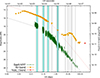 |
Fig. 5. Swift/XRT and optical light curves (MASTER CR band, X-shooter, GROND r′). Note that the optical data of the transient were obtained via image subtraction after 0.2 days, and therefore the contribution of the host is also subtracted. We highlight in cyan the epochs used in the optical-to-XRT SED fitting. Vertical lines highlight epochs with spectroscopic coverage. The dotted lines are the best fit of the optical light curve obtained in Section 4.2, which we have also normalised to the X-rays for data after 5 ks, i.e., excluding the first Swift orbit, which clearly shows that these early data are offset from the fit (see Sect. 4.3). |
Spectral energy distribution fit results.
These results agree with past findings on GRB afterglows (Ronchini et al. 2023). This event is among the 19 out of 30 GRBs analysed in that work, for which the shallow phase has an optical-to-X-ray spectrum fully consistent with synchrotron emission from a single population of shock accelerated electrons (Sample 1 in Ronchini et al. 2023). The mean X-ray luminosity during this phase is  erg s−1 and its duration is tb, X = 21.2 ks. Therefore, we infer a radiated isotropic energy of EX, iso = 1.3 × 1050 erg. By assuming a radiative efficiency of η ∼ 0.1 in agreement (e.g., Beniamini et al. 2016), we conclude that the bolometric isotropic kinetic energy of the jet is at least Ek, iso ∼ 1 × 1051 erg14.
4.4. Collimation-corrected energy
Under the assumptions of the scenario depicted above, we derive the half-opening angle of the jet. Assuming that the light curve break at 0.215 days (Table 2) represents the jet break (see Sect. 4.2), we use it to measure the collimation of the jet (Sari et al. 1999). Following (Frail et al. 2001) we calculated this angle using the following equation for a uniform jet expanding in a constant-density medium:
 (1)
(1)
where Etot, iso = Eγ, iso (Sect. 4.1, n = 1 cm−3 is the number density of the medium, η = Eγ, iso/Etot, iso = 0.215 is the typical radiative efficiency assumed for this calculation, tjet is the jet-break time, while z = 0.117 is the redshift of the event. We find θISM = 0.084 ± 0.003 rad (4.8 ± 0.2 deg), in agreement with other events (e.g., Laskar et al. 2014, 2018; Rossi et al. 2022a)16.
Using the above efficiency, we obtained Ek, iso = 1052 erg, consistent with the lower limit of Ek, iso > 1 × 1051 erg reported at the end of Sect. 4.3. If we consider the outflow to be collimated, the ‘true’ gamma-ray energy of the jet is Eγ = Eγ, iso(1 − cos(θjet)) ≃ 9 × 1048 erg. Therefore, we estimate the ‘total collimated energy’ of the jet to be Etot ≃ Eγ/η ≃ 0.4 × 1050 erg. Assuming a wind medium, and using the following equation from (Bloom et al. 2003):
 (2)
(2)
we obtained θwind = 0.126 ± 0.007 rad (7.2 ± 0.4 deg) and thus Etot ≃ 0.9 × 1050 erg.
4.5. Classification and bolometric light curve of the SN
To classify SN 2018fip, we compared our X-shooter spectra of SN 2018fip at 12, 18, and 23 days with other SNe using SNID (Blondin & Tonry 2011). We find that the broad-line features most closely match those of the broad-lined Type-Ic SN 2002ap at a compatible phase and the same redshift. For example, at 12 days the best match is obtained for −2.4 days relative to maximum light.
After separating the afterglow and SN contributions from the data as explained in Section 4.2, we constructed a bolometric light curve of the supernova emission using our g′r′i′z′J photometry. We analysed the light curve using the analytical model developed by Arnett (1982) for Type-Ia SNe, which can also be applied to core-collapse Type-Ic SNe with a few careful considerations: i) the model assumes spherical symmetry for the SN ejecta; ii) it assumes that the total amount of nickel is concentrated at the centre of the ejecta. These assumptions may not be appropriate in the case of highly rotating progenitor stars and asymmetric explosion (Cano et al. 2017b; Izzo et al. 2019), in which case the derived parameters can change significantly (e.g., Dessart et al. 2017). The model provides an estimate of the total kinetic energy of the SN ejecta, given the expansion velocity measured from P-Cygni absorption of spectral features around the peak brightness of the SN, as well as an estimate of the total amount of nickel synthesised in the explosion and the optical opacity. In particular, we derive the expansion velocity from the blueshift of the Fe II multiplets, along with the Si IIλ6355 doublet, O Iλ8446, and Ca II triplet λ8492 absorption features (Fig. 6), fitting each with a Gaussian profile, similarly to Modjaz et al. (2016). From the spectrum of the SN on rest-frame day 14 (12 days in observer frame), we inferred an expansion velocity of vej = 15 000 ± 1000 km s−1. With this assumption, the best fit to the bolometric light curve (Fig. C.1) with the Arnett model gives a total ejected mass in the SN of  M⊙, a kinetic energy of
  erg, and a synthesised nickel mass of
  M⊙, with a resulting opacity of k = 0.05 ± 0.02 cm2g−1. We find that SN 2018fip reaches a peak luminosity of (5.70 ± 0.41)×1042 erg s−1 at 14.9 ± 0.17 days after the GRB trigger (rest-frame).
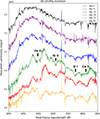 |
Fig. 6. Evolution of the spectra of SN 2018fip in the rest-frame. The absorption features marked in the image refer to the spectrum obtained about 5 days after the peak (day 18). Phases are in the observer frame. |
4.6. Spectral modelling of the SN
To remove the contribution of the afterglow and host from the spectra of SN 2018fip, we used our light-curve modelling to construct g′r′i′z′J SEDs at spectroscopic epochs after day 6 and subtracted them from the de-reddened spectra. Figure 6 shows the spectral evolution of SN 2018fip. We note that (Buckley et al. 2018) initially claimed an emerging SN based on spectroscopic data obtained 27.2 h after the burst with the SALT telescope. However, our second spectroscopic observation with VLT/X-shooter obtained 35.5 h (1.48 days) after the GRB (Heintz et al. 2018) does not show evidence of these broad undulations or deviations from a single power law with spectral index ∼0.7. The spectra remain featureless until the SN light-curve peak (day 12), when some absorption features start to appear. We performed spectral synthesis calculations using TARDIS (Kerzendorf & Sim 2014). Our reference model is shown in Figure 7. The input density structure for the reference model is shown in Fig. 8.
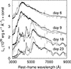 |
Fig. 7. Synthesised spectra as compared with those of SN 2018fip. Solid black lines represent the reference model spectra. The dashed black lines (on days 18 and 23) show the synthesised spectra with the high-velocity component included in the spectral synthesis calculations, demonstrating that this component is not present at late epochs. The observed spectra are shown with grey lines. The same constant in flux has been added for the model and data as an offset for presentation purposes (3.6, 2.0, 0.8, and 0.0 for day 6, 9, 18 and 23, respectively). |
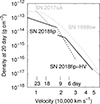 |
Fig. 8. Input density structure for the reference spectral model (solid black lines): the inner lower-velocity component for the spectra on day 18 and 23 (SN 2018fip) and the outer high-velocity component for day six and nine (SN 2018fip-HV). The dashed black line shows the upper limit set by the spectral synthesis analyses on days 18 and 23 (see the main text). The density structures derived for GRB-SNe 2017iuk (Izzo et al. 2019) and 1998bw (Iwamoto et al. 1998) are shown by solid grey and dashed grey lines, respectively. |
To study the temporal evolution, we started with the two spectra after SN peak observed on days 18 and 23. We first assume a density structure described by a single power law. We roughly constrain the photosphere position (i.e., set the photospheric velocity as the inner boundary for spectral synthesis) by requiring that the optical depth integrated back from the outer region to the photosphere is about unity for the putative opacity in the range of 0.03–0.6 cm2 g−1 that covers the C+O-rich to Fe-rich composition (Mazzali et al. 2001). Then, the photospheric velocity is varied within this range (Fig. 9), as well as the composition in the spectrum synthesis simulations. For the composition, we assume, for simplicity, that the relative mass fractions among Fe-peak elements produced by complete Si burning are universal, guided by typical results from explosive nucleosynthesis calculations (e.g., Maeda et al. 2002); X(56Ni):X(Ni):X(Fe):X(Co) = 0.1 : 0.013 : 0.01 : 0.007, where the normalisation here is set by the homogeneous mixing of all 56Ni (∼0.4 M⊙) over the entire ejecta (∼4 M⊙). The same is the case for Ti, Cr and Ca created by the incomplete Si burning; X(Ti):X(Cr):X(Ca) = 7 × 10⁻³ : 2 × 10⁻³ : 0.01. We vary the total abundance of these two element groups independently as parameters in the spectral synthesis. The remaining mass fractions are set to be those in a typical C+O-rich layer; a mixture of C, O, Mg together with a half of the solar abundance for the heavier elements as the progenitor abundance. We also varied the mass fractions of Si and S, but adding these elements above the progenitor values produced overly strong absorption features. Therefore, we set their additional contribution from explosive burning to zero for these elements; this is not unexpected if the explosive nucleosynthesis takes place following a jet-like explosion (e.g., Maeda & Nomoto 2003). In summary, for a given density structure, we have three main parameters: the photospheric velocity, the mass fraction of 56Ni (representing complete Si-burning products), and the mass fraction of Ca (representing incomplete Si-burning products).
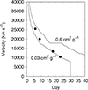 |
Fig. 9. Photospheric velocity used in the reference model (points). The two solid curves show the expected evolution of the photospheric velocity calculated for the reference density structure adopting a constant opacity of 0.03 or 0.6 cm2 g−1. In TARDIS spectral synthesis simulations, the input photospheric velocity is varied as a parameter within the range between the two lines shown here (see Sect. 4.6). |
After tuning these parameters to roughly match the observed spectra at days 18 and 23, we obtain our ‘final’ reference model for the low-velocity part of the ejecta up to ∼20 000 km s−1. We favour a shallow density distribution below ∼20 000 km s−1 (ρ ∝ v−2 in the reference model) for two reasons. First, reproducing the spectral evolution between days 18 and 23 requires a rapid decrease in the photospheric velocity. Second, the shallow density distribution reproduces line profiles that roughly match the observed spectra. As seen in Fig. 9, the photospheric velocities used in the model on day 18 and 23 satisfy the constraint from the optical depth. For the composition, our final values are X(56Ni) = 0.15 and X(Ca) = 0.003 below 15 000 km s−1 while X(56Ni) = 0.03 and X(Ca) = 6 × 10⁻⁴ above it (up to ∼20 000 km s−1). Although we do not aim to derive the composition structure accurately, the mass fractions of heavy elements appear to increase towards lower-velocity material, as expected from typical one-dimensional explosion simulations (e.g., Nomoto et al. 2006). The mass fractions of the Fe-peak elements in the inner region (15 000 km s−1) are roughly the values expected from homogeneous mixing.
We explored spectral synthesis simulations to identify ejecta structures that produce synthetic spectra roughly matching the spectra at the earlier epochs (days 6 and 9), independent of the structure applied to the later epochs. These spectra show strong suppression below ∼4000 Å and a largely featureless continuum. We explain these two features by a photosphere formed in a high-velocity, Fe-rich outer region (> 20 000 km s−1); in the reference model (Fig. 7), we set the 56Ni mass fraction to X(56Ni) = 0.24. The lower 56Ni content or lower photosheric velocity results in too blue a continuum without sufficient absorption in the blue portion of the spectra. One could keep the same 56Ni mass density in order to roughly create a similar amount of blue absorption by simultaneously decreasing X(56Ni) and increasing the density. However, this conflicts with the constraint on the photospheric velocity we set in our model construction (i.e., Fig. 9).
In the high-velocity region, we include stable Ni (i.e., 58Ni) with the relative mass fraction to 56Ni set the same as applied to the inner region. We do not include other Fe-peak elements or Ca in the high-velocity region, because they characteristic absorption features at different wavelength regions that clash with the observed featureless spectra. This indicates that this high-velocity component may originate in the highest-entropy region in the explosion (i.e., the one created in the deepest ejecta in a spherically symmetric configuration; Sato et al. 2021). The evolution of the photosphere and its velocity can be seen in Figures 8 and 9, which shows that the photosphere is in the high-velocity region early on, but is below the high-velocity region on day 18. We further discuss the implications in Section 5.2.
We note that the inner distribution adopted to model the spectra on day 18 and 23 does not include the high-velocity component used for the spectra on day 6 and 9. In ‘spectral tomography’ (e.g., Mazzali et al. 2015), the ejecta structure is reconstructed from the outermost to the innermost regions by modelling the early spectra first, since material above the photosphere can still significantly affect the observations. Figure 7 shows that this procedure does not work for SN 2018fip. The dashed curves are the synthetic spectra on day 18 and 23 created with the high-velocity outer component, showing several critical problems; the features dominated by Fe II at ∼5000 Å never match the data, with the pseudo emission peak shifted to the blue as compared to the observed wavelength, and the associated absorption becoming too strong. This indicates that there is too much (relatively low-temperature) Fe-rich material either along or out of the line of sight (for the absorption-emission problem). Also, the high-velocity component produces excessive absorption and heating in the outer layer, shifting the O I absorption towards higher velocities. Further details can be found in Appendix C.
4.7. The host galaxy
Thanks to our late imaging, we can investigate the morphology of the host galaxy. We used the last GROND epoch, obtained 254 days after the GRB, which is deeper than the X-shooter images. Unfortunately, also in this case the presence of the bright star disturbs the analysis. Therefore, we used the IRAF daophot package (Stetson 1987) to build a point spread function model and subtract the nearby star. After removing the emission from the star, an extended object is clearly visible at the afterglow/SN position in the optical bands (Fig. 10), which we identify as the host galaxy of GRB 180728A. The host appears to be made up of two bright regions visible in the g′ and r′ filters. It is extended in the SE-NW direction with major and minor axes of  and
and  , measured in the g′-band. These correspond to ∼3 and ∼1.4 kpc at the redshift of the GRB. The SE region is bluer and contributes approximately half of the host flux in the g′ band, indicating a younger stellar population than in the NW region. Interestingly, the bluer and younger SE-region does not coincide with the location of the GRB-SN (colour panel in Fig. 10), although the GRB exploded with a negligible offset from the brightest region, in agreement with the LGRB population (e.g., Bloom et al. 2002; Blanchard et al. 2016).
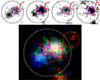 |
Fig. 10. RGB-colour image of the host galaxy of GRB 180728A, obtained from i′,r′ g′ images. Bluer regions correspond primarily to g′-band emission. The top panels show the individual g′ r′ i′ z′ GROND imaging. The nearby star (red circle) was removed using a point spread function model, although some residual is left. The magenta circle shows the position of the afterglow/SN. The dashed circle has a radius of 1 |

We obtained aperture photometry within a circular radius of  corresponding to 3.3 kpc at the redshift of the burst, large enough to include the entire host complex while avoiding nearby sources. The galaxy is not detected in the NIR bands with GROND down to the following AB upper limits J > 20.8, H > 19.7, Ks > 17.8, but it is detected in VISTA J archival images (though not in K). We measured the following AB aperture magnitudes, not corrected for the foreground Galactic extinction: g′ = 22.77 ± 0.06 , r′ = 22.40 ± 0.06 , i′ = 21.98 ± 0.09 , z′ = 21.67 ± 0.10, J = 21.4 ± 0.3. To assess whether the late-time data are still affected by SN light, we considered the SN 1998bw light curve, which extends beyond 250 days, together with the best-fit scaling and stretching parameters derived in Section 4.2. We find that the SN should be g = 25.5, r = 25, i = 24, z ∼ 24 which is 2–3 mag fainter than the host. This contribution is included in the photometric error of the host magnitude measurements.
To study the spectral properties of the host, we used the final spectrum obtained at 71 days, with the slit oriented along the host major axis. Since there was no detectable continuum in the NIR arm, we limited the analysis to the UVB and VIS arms. We accounted for the small SN contribution at this late epoch and fine-tuned the absolute flux calibration using late-time g′, r′, i′, and z′ GROND photometry at 254 days (see below), which is free from SN and afterglow emission. The continuum of the host galaxy is clearly detected between 0.4 μm−1 μm. We detect the emission lines [O III] doublet and [N II], Balmer Hβλ4861 and Hαλ6563 (Fig. 11) at a redshift of 0.1172 ± 0.0001, consistent with that of the afterglow (Sect. 3.2). All measured fluxes are reported in Table 4. Since the slit follows the host major axis, it captures emission from both star-forming regions (Fig. 10). Following the O3N2 metallicity calibration from Hirschauer et al. (2018), we find 12 + log(O/H) = 8.57. The Balmer decrement, Hα/Hβ = 2.61 ± 0.36, corresponds to AV < 0.1 and therefore to a negligible dust content (Osterbrock 1989). We measure a low star formation rate (SFR) of 0.02 M⊙/yr based on the Hα line flux, assuming a (Chabrier 2003) initial mass function and following Treyer et al. (2007). The low SFR and metallicity are consistent with those observed for LGRB hosts at similar redshifts (e.g., Krühler et al. 2015; Vergani et al. 2015; Japelj et al. 2016).
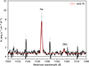 |
Fig. 11. Zoom-in on the Hα line and [N II] region of the VLT/X-shooter spectrum of the host galaxy in units of 10−17 erg s−1 cm−2 Å−1. The detected emission lines are marked. A fit of the lines and of the continuum is shown in red. In grey is the error on the spectrum. |
Emission lines fluxes corrected for Galactic extinction.
After correcting for foreground extinction, we modelled the host-galaxy SED with the CIGALE code (Boquien et al. 2019), fixing the redshift to z = 0.117. Unfortunately, the photometric uncertainties prevented us from modelling the two regions separately. Given the lack of rest-frame UV photometry, it is also difficult to constrain the SFR. We can still estimate the SFR using an alternative approach: in i′ the host is brighter than in r′ and z′-bands, which we interpret as Hα emission falling within this band at the redshift of the GRB (Fig. 12). We include this effect in the SED fitting because CIGALE accounts for the contribution of emission lines to the photometry via Kennicutt relations (Kennicutt 1998), allowing an SFR estimate, although the large photometric uncertainties make this constraint very uncertain. Assuming a delayed star formation history and a Bruzual & Charlot (2003) stellar population with a Chabrier initial mass function, we obtain a best fit to the photometric data ( ) for a galaxy with a relatively young (0.3–0.9 Gyr) stellar population, dust attenuation AV = 0.4 mag (using the Calzetti et al. 2000 law), a stellar mass of 107.84 ± 0.23 M⊙, SFR of
  , i.e.,
  . With these values we derive a specific SFR (SSFR) of 0.1–9 Gyr−1, well within those measured so far in the LGRB host population (e.g., Savaglio et al. 2009; Hunt et al. 2014; Perley et al. 2013; Vergani et al. 2015; Japelj et al. 2016; Schulze et al. 2018). The absolute magnitude is MB = −16. We conclude that this is a young star-forming dwarf galaxy similar to other LGRB host galaxies found at low redshift (e.g., Savaglio et al. 2009; Taggart & Perley 2021). In particular, its properties are similar to the host of GRB 030329, which is just slightly more luminous (MB ∼ −17; Gorosabel et al. 2005; Sollerman et al. 2005; Savaglio et al. 2009).
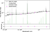 |
Fig. 12. GROND g′ r′ i′ z′ and VISTA J-band photometry of the host galaxy of GRB 180728A with Cigale (Section 4.7). The best model (solid line) is shown together with the relative residuals. Photometric measurements are marked by violet empty circles. |
5. Discussion
5.1. The afterglow of GRB 180728A in context
Using the redshift and the SED, we transform the pure afterglow light curve to z = 1 following the method described in (Kann et al. 2006). Here, we correct the afterglow for line-of-sight extinction (negligible in this case) and shift it in time and luminosity to z = 1, including the k-correction. The magnitude offset we find is dRc = +5.23 ± 0.03. Thereby, it can be directly compared to the large afterglow collection presented by (Kann et al. 2006, 2010, 2011, 2024b). We show the comparison in Fig. 13, with the afterglow of GRB 180728A highlighted in red. We also highlight with thicker dark grey lines the afterglows of some other GRBs at z < 0.5 that are associated with GRB-SNe (spectroscopically secure in most cases), where some are labelled.
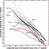 |
Fig. 13. Afterglows of GRBs, all transformed to the z = 1 system following the method of Kann et al. (2006). We highlight (in red) the afterglow of GRB 180728A, which is seen to be among the faintest known in the context of luminosity. We also mark with thick dark grey lines other GRBs at z < 0.5 that are associated with SNe (the SN emission has been subtracted in this plot). |
Similarly, to place the X-ray emission of GRB 180728A in context, we retrieved X-ray light curves of all Swift GRBs up to February 2024 with detected afterglows (at least two epochs) and known redshifts from the Swift Burst Analyser17 (Evans et al. 2010). The density plot in Fig. 14 displays the parameter space occupied by these 473 bursts (using the method described in Schulze et al. 2014). In this case, for comparison, we have also highlighted other GRBs with spectroscopically confirmed SNe and separated them in low- and high-Eγ, iso18. From these figures, it can be seen that the optical afterglow of GRB 180728A, while bright observationally, is among the least luminous known. Definite SN-associated GRBs have early afterglows that range from typical to faint. Indeed, several of these are among the faintest afterglows ever followed up to late times; this is a selection bias stemming from the interest in SN follow-up combined with Swift’s capability to probe the UV regime where GRB-SNe are usually strongly suppressed (but see Kann et al. 2019), revealing the true afterglow evolution.
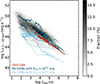 |
Fig. 14. X-ray light curve of GRB 180728A in the context of the X-ray afterglows of 473 Swift GRBs with known redshifts (until February 2024). For comparison, we overlay the light curves of Swift GRBs with spectroscopically confirmed SNe and divide the sample into six SN-GRBs with Eγ, iso < 1051 and nine SN-GRBs with Eγ, iso > 1051 erg. The colour table on the right side translates a grey shade at a given luminosity and time into a fraction of bursts. |
As in the optical, the X-ray afterglow of GRB 180728A is slightly underluminous compared to other Swift GRBs, although it is not among the faintest, as in three other events the X-ray afterglow declines rapidly without the early shallow phase observed here. However, we see that GRB 180728A lies in between the two samples of high-energy cosmological GRBs and low-energy and low-redshift GRBs, especially within one day. Therefore, in this case, the X-ray afterglow appears to scale with Eγ, iso. Hu et al. (2021) noted that its Swift/XRT light curve shows late-time bumps at 10 keV that are also observed in the cases of GRBs 190829A and 171205A (Izzo et al. 2019), although bumps are known since at least GRB 030329 (e.g., Zeh et al. 2004) and are a possible signature of refreshed shocks (e.g., Granot et al. 2003; Moss et al. 2023).
In fact, a striking difference from other GRB-SNe at z < 0.5 is in the slower fading of the afterglow (see Figs. 13 and 14) within the first 0.1 days. None of the other low-redshift GRB-SNe show such early shallow fading except for GRB 091127-SN2009nz (Filgas et al. 2011), which has a light curve that is strikingly similar though ≈10 times more luminous. Indeed, both the prompt emission and the SN are more luminous than those of GRB 180728A/SN 2018fip and are more similar to those of GRB 030329/SN 2003dh. Not surprisingly, at late times (> 1 day in rest frame) almost all afterglows show a similar decay after the jet break (an exception being GRB 1304027A, see e.g., De Pasquale et al. 2016).
5.2. The asphericity and energy of the SN ejecta
In Section 4.6, we modelled the spectroscopic data from 6 to 23 days using a high-velocity component for the early phase and a low-velocity component for the late phase. A problem we found is that the high-velocity component must produce detectable signatures at later epochs, but no such traces are seen on day 18 and thereafter. This discrepancy may have important implications for the ejecta structure, the jet formation, and the explosion mechanism. The most likely cause of the problem in explaining the spectral evolution is the strong assumption of spherical symmetry adopted in TARDIS. In fact, asymmetry/asphericity in the ejecta structure has been extensively discussed for GRB-SNe (e.g., Maeda & Nomoto 2003; Suzuki & Maeda 2022; Maeda et al. 2023). One possible configuration that could overcome this problem/difficulty is the one shown in Figure 15: a combination of a 56Ni-rich high-velocity component confined in a narrow solid angle and a slower quasi-spherical ejecta (see also Ashall et al. 2019). In this configuration, the photosphere is within the high-velocity 56Ni-rich component in the early phase (when the radiation output can indeed be dominated by this component; Maeda et al. 2006), while it recedes to the inner ejecta component in the late phase. If the solid angle of the high-velocity component is significantly smaller than the size of the photosphere in the late phase, the absorption created in the high-velocity component could be minimised. If we take the characteristic velocity of the high-velocity component as ∼20 000 km s−1 and the photospheric velocity on day 23 as ∼10 000 km s−1 (Fig. 9), this requires that the half-opening angle of the high-velocity component is < 30°, or the fraction of the solid angle (Ω/4π) < 13% assuming the bipolar structure. The high-velocity Fe-rich component may represent a sub-relativistic cocoon associated with a GRB jet (Nakar 2015; Nakar & Piran 2017; Gottlieb et al. 2018; Piro & Kollmeier 2018; Izzo et al. 2019).
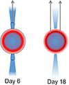 |
Fig. 15. Schematic of the ejecta structure, showing a combination of the 56Ni-rich high-velocity component confined in a narrow solid angle and the slower quasi-spherical ejecta. The black line shows the photosphere at: i) 6 days, when it includes the high-velocity high-velocity component, and ii) at 18 days, when the photosphere recedes in the inner ejecta. |
The low-velocity (perhaps quasi-spherical) component has the ejecta mass Mej, kinetic energy Ek, SN, and Nickel mass M(56Ni) within ∼10 000 − 20 000 km s−1 as follows: ∼1.5 M⊙, ∼3 × 1051 erg, and ∼0.17 M⊙, respectively. Because it does not include material below ∼10 000 km s−1 and above 20 000 km s−1, these values provide lower limits. For example, incorporating the density structure above 20 000 km s−1 (dashed line in Fig. 8) increases them to Mej ∼ 2 M⊙ and ∼5 × 1051 erg. On the other hand, the high-velocity component (> 20 000 km s−1) has isotropic values of Mej ∼ 0.5 M⊙, ∼3.5 × 1051 erg, and M(56Ni) ∼0.1 M⊙. Because the high-velocity component occupies a narrow solid angle, the low-velocity component likely dominates the total mass and energy. A fair comparison to other GRB-SNe (whose values are usually derived through the Arnett relation) requires care, because asphericity strongly affects the spectral properties of SN 2018fip, particularly its energy. If we assume a simple spherical scenario, we can sum the inner and outer components obtained above, with an additional hidden internal region of 1 M⊙, and therefore obtain a total of Mej = 3 M⊙ and Ek, SN ∼ 6.5 × 1051 erg. Note that the low-velocity ejecta agree well with the values obtained via the bolometric light curve and the Arnett model, probably because both methods assume a homologous expansion with nickel concentrated in the centre. The high-velocity ejecta adds additional energy, and thus the total values are larger than those obtained from the bolometric light curve. However, the kinetic energy estimated for the high-velocity component could be overestimated and should be reduced by a factor < 0.13, considering the half-opening angle of < 30° estimated above.
5.3. The energetics of GRB 180728A/SN 2018fip in context
The photometric data (Fig. 3) reveals a light curve that smoothly decays after a peak, then breaks into a steeper decay, and finally gives over to the rising associated supernova SN 2018fip. The light curve evolution strongly resembles GRB 011121 (Greiner et al. 2003). It is less similar to well-known nearby GRB-SN associations such as GRB 030329 – SN 2003dh (Stanek et al. 2003; Hjorth et al. 2003; Matheson et al. 2003), where the afterglow brightness suppresses the SN bump’s visibility. Similarly, low-energy events such as XRF 060218/SN 2006ap (Campana et al. 2006; Pian et al. 2006; Ferrero et al. 2006) and GRB 171205A – SN 2017iuk (Izzo et al. 2019), show a clear SN bump but essentially no afterglow emission.
Figure 16 shows the quasi-bolometric light curve of SN 2018fip compared to the 13 GRB-SNe, with low-order spline fits overplotted for clarity. Details regarding the selection criteria for the comparison sample and the methodology used to estimate their bolometric light curves are described in Kumar et al. (2024). The comparison sample consists of 13 well-observed GRB-SNe, whose light curves are compiled primarily from Cano et al. (2017b) and references therein, along with more recent events such as SN 2016jca (Cano et al. 2017a; Ashall et al. 2019), SN 2017htp (de Ugarte Postigo et al. 2017; Melandri et al. 2019; Kumar et al. 2022), SN 2017iuk (Wang et al. 2018; Izzo et al. 2019; Suzuki et al. 2019; Kumar et al. 2022), and SN 2019jrj (Melandri et al. 2022). The full sample spans a wide range of peak quasi-bolometric luminosities, from ∼3 to 36 × 1042 erg s−1 (Kumar et al. 2024). SN 2018fip reaches a peak luminosity of ∼5.7 × 1042 erg s−1 at ≈15 days post-burst, placing it on the fainter end of the GRB-SN luminosity distribution. This highlights the considerable diversity in GRB-SN energetics and positions SN 2018fip as an intrinsically low-luminosity example within the population. Notably, this comparison is conducted without rescaling to SN 1998bw, allowing for a direct interpretation of absolute luminosity differences across the sample.
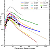 |
Fig. 16. Quasi-bolometric light curve of SN 2018fip compared to those of 13 well-observed GRB-SNe, with low-order spline fits shown for each. Most of the comparison light curves, especially for GRB-SNe observed before 2015, are adopted from the compilation by Cano et al. (2017b), which incorporates data from multiple earlier studies cited therein. Additional events were included from more recent works by Cano et al. (2017a), Izzo et al. (2019), Melandri et al. (2019, 2022), Kumar et al. (2022, 2024). |
To further compare the light curves of SN 2018fip with those of other GRB SNe, we used the parametrisation k,s19 (top panel of Fig. 17 and Section 4.2). SN 2018fip lies in the middle of the k,s space covered by GRB-SNe. Therefore, it is one of the nearest SNe in the k,s space to the prototype SN 1998bw. The most similar case is GRB 140606B, which also has a similar isotropic energy. The faint and early peaking end of the diagram (bottom-left) is occupied by the notable cases of SN 2010bh/GRB 100316D (Starling et al. 2011; Bufano et al. 2012; Olivares et al. 2015) and SN 2006aj/GRB 060218 (Ferrero et al. 2006). At the luminous/late-peaking end lies 2011kl/GRB111209B, but we note that this event is more similar spectroscopically to superluminous supernovae (Greiner et al. 2015; Kann et al. 2019). We do not show the BOAT GRB 221009A in the figures because its associated supernova SN 2022xiw cannot be thoroughly studied, although observations suggest that it was less luminous than SN 1998bw (e.g., Blanchard et al. 2024; Fulton et al. 2023; Levan et al. 2023; Kong et al. 2024; Shrestha et al. 2023; Srinivasaragavan et al. 2023).
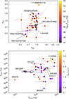 |
Fig. 17. Top: Luminosity–stretch diagram colour-coded by Eγ, iso. The dashed line is the best fit from (Klose et al. 2019). Bottom:Ek, SN – Eγ, iso plane, colour-coded by T90. Data are from (Cano et al. 2017b) and have been updated with recent results (Klose et al. 2019; Dainotti et al. 2022; Kann et al. 2024a; Dong et al. 2025). For SN 2018fip, the error on Ek, SN obtained via the Arnett modelling extends up to the one obtained by the spectral modelling and spherical approximation. |
In the bottom panel in Figure 17 we compare all GRBs with a known SN in the Ek, SN – Eγ, iso plane, (data from Minaev & Pozanenko 2020; Tsvetkova et al. 2021; Demianski et al. 2018; Dainotti et al. 2022, thus limited to this about 2021). For SN 2018fip, we also consider the additional contribution of the high-velocity component obtained by spectral modelling, but still in a spherical approximation (Section 5.2). GRB radiated energy (not corrected for collimation) spans more than 6 orders of magnitude, with the recent BOAT being an extreme example (Burns et al. 2023; Frederiks et al. 2023). As already known, most GRB-SNe have Ek, SN ∼ 1052–1053 erg (not corrected for asymmetry, see Mazzali et al. 2014; Ashall et al. 2019; Melandri et al. 2019), regardless of the GRB energy, suggesting that the GRB-SN phenomenon is driven by the SN, not the GRB jet (e.g., Woosley & Bloom 2006; Mazzali et al. 2014). SN 2018fip is towards the low-energy side of this plane, below 1052 erg, which means that overall not an extreme amount of energy resulted from the death of this massive star. This could even double if one considers the additional energy of the high-velocity ejecta, although this is likely highly collimated, and thus must be considered an upper limit. Considering the events at z < 0.2, it we find it interesting to compare GRB 180728A with the well-studied GRB 030229, again omitting the weakly constrained SN 2022xiw of GRB 221009A. The top panel shows that SN 2003dh is one of the brightest supernovae, 3 times more luminous, though peaking at similar times as SN 2018fip (see Fig. 17). The bottom panel shows that it has Ek, SN ≳ 5 − 10 times that of SN 2018fip.
Lü et al. (2018) have estimated the energy partition within GRB-SNe, defined as the GRB efficiency ξ% = Etot/(Etot + Ek, SN)20, where Etot is the total collimated energy of the jet (Section 4.4). They confirmed previous results showing that in these systems the beaming-corrected GRB energy is usually smaller than the SN energy, with less than 30% of the total energy distributed in the relativistic jet. It is likely that the real distribution is less skewed towards lower values, because in many cases only lower limits exist (for details, see Lü et al. 2018). For GRB 180728A/SN 2018fip, using the total collimated energy estimated in Section 4.4 and the SN energy found in Section 5.2, we find that the efficiency of GRB 180728A is ∼2%21. Considering the assumptions made (see Sections 4.4 and 4.3), this is a qualitative value that enables comparison with other GRB-SNe. Similarly to the results obtained by Lü et al. (2018), we find that the low efficiency of this event is similar to the majority of GRB-SNe, where only GRB 111209A stands out22 (Fig. 18). Please note again that in these considerations GRBs are already corrected for the collimation, but the asphericity of SNe is not considered. In general, for a correct comparison, all events should be modelled considering a high-velocity component (see, e.g. Khatami & Kasen 2019) and also corrected for asphericity, but this is possible only for very few events (e.g. Ashall et al. 2019).
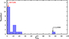 |
Fig. 18. Distribution of the GRB efficiency ξ% following the approach described in Lü et al. (2018). We highlight GRBs 180728A/SN 2018fip and 111209A/SN 2011kl, which are discussed in the text. |
In the bottom panel of Figure 17, we show in purple all GRBs with a duration shorter than ∼20 s (the average LGRB duration (e.g., Minaev & Pozanenko 2020; Tsvetkova et al. 2021), and we observe that they typically have Eγ, iso < 1053 erg. Assuming that Eγ, iso is a reasonable good proxy for the total GRB jet energy (or, in other words, assuming universal efficiency), this can be partly explained in the context of the collapsar scenario. In this model, only the longest GRBs (those with the longest engines) retain sufficient energy after breaking out from the stellar envelope to power the GRB jet (e.g., Lazzati et al. 2013). Indeed, we notice that, in general, GRB 180728A is in the central part of the figure, in agreement with the aforementioned collapsar scenario and the short duration of just 8.7 s. Notably, GRB 180728A has one of the shortest durations among GRB-SNe, along with GRB 091127 (7.42 s), which also exhibits a similar afterglow, as noted in Sect. 5.1. GRB 091127 has similar efficiency (ξ% ≲ 8), a slightly more energetic SN (Ek, SN ∼ 13 × 1051 erg), and a very similar afterglow evolution, suggesting that it had a progenitor and engine similar to those of GRB 180728A. However, its afterglow was four magnitudes more luminous, making the SN-bump less evident (Cobb et al. 2010; Olivares et al. 2015).
6. Summary and conclusions
GRB 180728A is a long-duration GRB detected at redshift z = 0.117. It is notable for its high isotropic energy release Eγ, iso > 1051 erg, making it one of the nearest high-energy GRBs ever observed at low redshift (z < 0.2), similar to GRB 030329. We used multi-band photometric and spectroscopic observations up to 80 days post-burst and applied image subtraction to isolate the SN light from a nearby star. This is one of only a handful of events detected in the J-band. We analysed the prompt and afterglow emission and host-galaxy spectra, and spectral synthesis of the SN was done using TARDIS. We then compared GRB 180728A/SN 2018fip with other events to investigate correlations between GRB energy and SN properties. In the following, we summarise our key results.
-
The GRB has an isotropic energy Eγ, iso of (2.5 ± 0.5)×1051 erg and an intrinsic spectral peak energy Ep, i of 123 ± 28 keV.
-
The afterglow exhibits a slow early fading followed by a break at 0.2 days. It was slightly underluminous, placing it between high-energy cosmological GRBs and low-energy nearby GRBs.
-
The host is an irregular low-mass blue star-forming galaxy, which is typical for low-z collapsar events.
-
The SN 2018fip spectral modelling indicates aspherical explosion with a two-component ejecta: a narrow, high-velocity outer layer more dominant during the early spectra (5–8 days in the rest-frame) with a velocity above 20 000 km s−1, and a slower (15 000 km s−1) more massive inner spherical component more dominant in later spectra (16–21 days in the rest-frame). The high-velocity component is likely confined to < 30°, and it plays a crucial role in explaining the evolution of SN 2018fip.
-
Assuming a quasi-spherical scenario, the spectral modelling yielded a total ejected mass of Mej = 3 M⊙ and a kinetic energy of Ek, SN ∼ 6.5 × 1051 erg. The symmetric spherical model of Ni-radioactive-heating of Arnett (1982), gives
 M⊙,
M⊙,  M⊙, and
  erg.
erg. -
SN 2018fip is a a broad-lined Type Ic with a kinetic energy just below the common range of 1052–1053 erg typical for GRB-SNe.
In conclusion, despite its high energy, GRB 180728A is associated with a supernova and afterglow that are intrinsically fainter than those of typical events. Indeed, although its burst energy is comparable to that of GRB 030329, both its afterglow and supernova are significantly fainter, highlighting the diversity in GRB-SN properties even at similar redshifts and energies. Overall, the low GRB efficiency of 180728A (∼2%) is similar to most GRB-SNe, reinforcing the view that these explosions are powered primarily by the supernova rather than the GRB jet. Finally, our results reinforce earlier findings on the asphericity of GRB–SN explosions and emphasise its crucial role in shaping the true energetics. The upcoming extremely large telescopes and the James Webb Space Telescope (McGuire et al. 2016) will enable high-quality multi-epoch spectroscopy of GRB-SNe beyond z ∼ 0.2, expanding the sample available for advanced spectral modelling, including studies of asymmetry, and allowing for investigation of the higher-energy GRBs typical at cosmological distances.
Data availability
The full Table C.3 is available at the CDS via https://cdsarc.cds.unistra.fr/viz-bin/cat/J/A+A/708/A60. The reduced and flux calibrated spectra are available on the ESO Science Archive Facility as data collection GRB180728A_SN2018fip23. The absolute-flux calibrated, extinction corrected, and afterglow subtracted spectra of SN 2018fip are available on the Weizmann Interactive Supernova Data Repository24 (WISeREP).
Acknowledgments
We thank the anonymous referee for providing thoughtful comments. A. Rossi thanks P. Evans for his help in the analysis of the Swift/XRT data. A. Rossi and E. Palazzi acknowledge financial support from PRIN-MIUR 2017 (grant 20179ZF5KS) and from the INAF project ‘Supporto Arizona & Italia’. L. Izzo acknowledges financial support from the INAF Data Grant Program ‘YES’ (PI: Izzo) ‘Multi-wavelength and multi messenger analysis of relativistic supernovae’. K. Maeda acknowledges support from the Japan Society for the Promotion of Science (JSPS) KAKENHI grants JP24KK0070, JP24H01810, and JP20H00174. The spectral mdoeling calculations were in part carried out on Yukawa-21 at YITP in Kyoto University. DBM is funded by the European Union (ERC, HEAVYMETAL, 101071865). Views and opinions expressed are, however, those of the authors only and do not necessarily reflect those of the European Union or the European Research Council. Neither the European Union nor the granting authority can be held responsible for them. The Cosmic Dawn Center (DAWN) is funded by the Danish National Research Foundation under grant DNRF140. AK is supported by the UK Science and Technology Facilities Council (STFC) Consolidated grant ST/V000853/1. R.B acknowledges funding from the Italian Space Agency, contract ASI/INAF n. I/004/11/6. The research leading to these results has received funding from the European Union’s Horizon 2020 Programme under the AHEAD2020 project (grant agreement n. 871158). Part of the funding for GROND (both hardware and personnel) was generously granted by the Leibniz-Prize to G. Hasinger (DFG grant HA 1850/28-1) and by the Thüringer Landessternwarte Tautenburg. The VL, PB, DV study was conducted under the state assignment of Lomonosov MSU. This work made use of WISeREP – https://www.wiserep.org. This research has made use of the NASA/IPAC Infrared Science Archive, which is funded by the National Aeronautics and Space Administration and operated by the California Institute of Technology. This work made use of data supplied by the UK Swift Science Data Centre at the University of Leicester. This research made use of TARDIS, a community-developed software package for spectral synthesis in supernovae. The development of TARDIS received support from GitHub, the Google Summer of Code initiative, and ESA’s Summer of Code in Space program. TARDIS is a fiscally sponsored project of NumFOCUS. TARDIS makes extensive use of Astropy and Pyne. This work is based on observations collected at the Very Large Telescope of the European Southern Observatory, Paranal, Chile (ESO programmes 2101.D-5044, PI: A. Rossi; 0101.D-0648, PI: N. Tanvir).
References
- Abbott, B. P., Abbott, R., Abbott, T. D., et al. 2017a, Phys. Rev. Lett., 119, 161101 [Google Scholar]
- Abbott, B. P., Abbott, R., Abbott, T. D., et al. 2017b, ApJ, 848, L12 [Google Scholar]
- Ahumada, T., Singer, L. P., Anand, S., et al. 2021, Nat. Astron., 5, 917 [NASA ADS] [CrossRef] [Google Scholar]
- Amati, L. 2006, MNRAS, 372, 233 [Google Scholar]
- Amati, L., Frontera, F., Tavani, M., et al. 2002, A&A, 390, 81 [NASA ADS] [CrossRef] [EDP Sciences] [Google Scholar]
- Amati, L., D’Agostino, R., Luongo, O., Muccino, M., & Tantalo, M. 2019, MNRAS, 486, L46 [CrossRef] [Google Scholar]
- Arnaud, K. A. 1996, ASP Conf. Ser., 101, 17 [Google Scholar]
- Arnett, W. D. 1982, ApJ, 253, 785 [Google Scholar]
- Ashall, C., Mazzali, P. A., Pian, E., et al. 2019, MNRAS, 487, 5824 [NASA ADS] [CrossRef] [Google Scholar]
- Barthelmy, S. D., Barbier, L. M., Cummings, J. R., et al. 2005, Space Sci. Rev., 120, 143 [Google Scholar]
- Becker, A. 2015, Astrophysics Source Code Library [record ascl:1504.004] [Google Scholar]
- Beniamini, P., Nava, L., Duran, R. B., & Piran, T. 2015, MNRAS, 454, 1073 [NASA ADS] [CrossRef] [Google Scholar]
- Beniamini, P., Nava, L., & Piran, T. 2016, MNRAS, 461, 51 [NASA ADS] [CrossRef] [Google Scholar]
- Bertin, E., & Arnouts, S. 2010, Astrophysics Source Code Library [record ascl: 1010.064] [Google Scholar]
- Beuermann, K., Hessman, F. V., Reinsch, K., et al. 1999, A&A, 352, L26 [NASA ADS] [Google Scholar]
- Blanchard, P. K., Berger, E., & Fong, W.-F. 2016, ApJ, 817, 144 [Google Scholar]
- Blanchard, P. K., Villar, V. A., Chornock, R., et al. 2024, Nat. Astron., 8, 774 [NASA ADS] [CrossRef] [Google Scholar]
- Blondin, S., & Tonry, J. L. 2011, Astrophysics Source Code Library [record ascl:1107.001] [Google Scholar]
- Bloom, J. S., Kulkarni, S. R., & Djorgovski, S. G. 2002, AJ, 123, 1111 [NASA ADS] [CrossRef] [Google Scholar]
- Bloom, J. S., Frail, D. A., & Kulkarni, S. R. 2003, ApJ, 594, 674 [NASA ADS] [CrossRef] [Google Scholar]
- Boquien, M., Burgarella, D., Roehlly, Y., et al. 2019, A&A, 622, A103 [NASA ADS] [CrossRef] [EDP Sciences] [Google Scholar]
- Bromberg, O., Nakar, E., Piran, T., & Sari, R. 2012, ApJ, 749, 110 [NASA ADS] [CrossRef] [Google Scholar]
- Bruzual, G., & Charlot, S. 2003, MNRAS, 344, 1000 [NASA ADS] [CrossRef] [Google Scholar]
- Buckley, D. A. H., Potter, S. B., Lipunov, V., et al. 2018, ATel, 11897, 1 [Google Scholar]
- Bufano, F., Pian, E., Sollerman, J., et al. 2012, ApJ, 753, 67 [Google Scholar]
- Burns, E., Svinkin, D., Fenimore, E., et al. 2023, ApJ, 946, L31 [NASA ADS] [CrossRef] [Google Scholar]
- Burrows, D. N., Hill, J. E., Nousek, J. A., et al. 2005, Space Sci. Rev., 120, 165 [Google Scholar]
- Calzetti, D., Armus, L., Bohlin, R. C., et al. 2000, ApJ, 533, 682 [NASA ADS] [CrossRef] [Google Scholar]
- Campana, S., Mangano, V., Blustin, A. J., et al. 2006, Nature, 442, 1008 [NASA ADS] [CrossRef] [Google Scholar]
- Cano, Z., Izzo, L., de Ugarte Postigo, A., et al. 2017a, A&A, 605, A107 [NASA ADS] [CrossRef] [EDP Sciences] [Google Scholar]
- Cano, Z., Wang, S.-Q., Dai, Z.-G., & Wu, X.-F. 2017b, Adv. Astron., 2017, 8929054 [CrossRef] [Google Scholar]
- Cardelli, J. A., Clayton, G. C., & Mathis, J. S. 1989, ApJ, 345, 245 [Google Scholar]
- Chabrier, G. 2003, PASP, 115, 763 [Google Scholar]
- Chevalier, R. A., & Li, Z.-Y. 1999, ApJ, 520, L29 [NASA ADS] [CrossRef] [Google Scholar]
- Clocchiatti, A., Suntzeff, N. B., Covarrubias, R., & Candia, P. 2011, AJ, 141, 163 [NASA ADS] [CrossRef] [Google Scholar]
- Cobb, B. E., Bloom, J. S., Perley, D. A., et al. 2010, ApJ, 718, L150 [NASA ADS] [CrossRef] [Google Scholar]
- Covino, S., Zerbi, F. M., Chincarini, G., et al. 2004, Astron. Nachr., 325, 543 [NASA ADS] [CrossRef] [Google Scholar]
- Dainotti, M. G., De Simone, B., Islam, K. M., et al. 2022, ApJ, 938, 41 [Google Scholar]
- D’Avanzo, P., Salvaterra, R., Sbarufatti, B., et al. 2012, MNRAS, 425, 506 [CrossRef] [Google Scholar]
- De Pasquale, M., Page, M. J., Kann, D. A., et al. 2016, MNRAS, 462, 1111 [NASA ADS] [CrossRef] [Google Scholar]
- de Ugarte Postigo, A., Selsing, J., Malesani, D., et al. 2017, GCN, 22096, 1 [Google Scholar]
- Demianski, M., Piedipalumbo, E., Sawant, D., & Amati, L. 2018, Mem. Soc. Astron. It., 89, 197 [Google Scholar]
- Dessart, L., John Hillier, D., Yoon, S.-C., Waldman, R., & Livne, E. 2017, A&A, 603, A51 [NASA ADS] [CrossRef] [EDP Sciences] [Google Scholar]
- Devillard, N. 1997, Messenger, 87, 19 [Google Scholar]
- Dong, X.-F., Huang, Y.-F., Zhang, Z.-B., et al. 2025, ApJ, 993, 20 [Google Scholar]
- Evans, P. A., Beardmore, A. P., Page, K. L., et al. 2007, A&A, 469, 379 [NASA ADS] [CrossRef] [EDP Sciences] [Google Scholar]
- Evans, P. A., Beardmore, A. P., Page, K. L., et al. 2009, MNRAS, 397, 1177 [Google Scholar]
- Evans, P. A., Willingale, R., Osborne, J. P., et al. 2010, A&A, 519, A102 [NASA ADS] [CrossRef] [EDP Sciences] [Google Scholar]
- Ferrero, P., Kann, D. A., Zeh, A., et al. 2006, A&A, 457, 857 [NASA ADS] [CrossRef] [EDP Sciences] [Google Scholar]
- Filgas, R., Greiner, J., Schady, P., et al. 2011, A&A, 535, A57 [NASA ADS] [CrossRef] [EDP Sciences] [Google Scholar]
- Frail, D. A., Kulkarni, S. R., Sari, R., et al. 2001, ApJ, 562, L55 [NASA ADS] [CrossRef] [Google Scholar]
- Frederiks, D., Golenetskii, S., Aptekar, R., et al. 2018, GCN, 23061, 1 [Google Scholar]
- Frederiks, D., Svinkin, D., Lysenko, A. L., et al. 2023, ApJ, 949, L7 [NASA ADS] [CrossRef] [Google Scholar]
- Fulton, M. D., Smartt, S. J., Rhodes, L., et al. 2023, ApJ, 946, L22 [NASA ADS] [CrossRef] [Google Scholar]
- Gaia Collaboration (Brown, A. G. A., et al.) 2018, A&A, 616, A1 [NASA ADS] [CrossRef] [EDP Sciences] [Google Scholar]
- Galama, T. J., Vreeswijk, P. M., van Paradijs, J., et al. 1998, Nature, 395, 670 [Google Scholar]
- Gehrels, N., Chincarini, G., Giommi, P., et al. 2004, ApJ, 611, 1005 [Google Scholar]
- Gorosabel, J., Pérez-Ramírez, D., Sollerman, J., et al. 2005, A&A, 444, 711 [NASA ADS] [CrossRef] [EDP Sciences] [Google Scholar]
- Gottlieb, O., Nakar, E., Piran, T., & Hotokezaka, K. 2018, MNRAS, 479, 588 [NASA ADS] [Google Scholar]
- Granot, J., Nakar, E., & Piran, T. 2003, Nature, 426, 138 [Google Scholar]
- Greiner, J., Klose, S., Salvato, M., et al. 2003, ApJ, 599, 1223 [NASA ADS] [CrossRef] [Google Scholar]
- Greiner, J., Bornemann, W., Clemens, C., et al. 2008, PASP, 120, 405 [Google Scholar]
- Greiner, J., Mazzali, P. A., Kann, D. A., et al. 2015, Nature, 523, 189 [Google Scholar]
- Heintz, K. E., Izzo, L., Rossi, A., et al. 2018, GCN, 23067, 1 [Google Scholar]
- Hirschauer, A. S., Salzer, J. J., Janowiecki, S., & Wegner, G. A. 2018, AJ, 155, 82 [NASA ADS] [CrossRef] [Google Scholar]
- Hjorth, J. 2013, Philos. Trans. R. Soc. Lond. Ser. A, 371, 20120275 [Google Scholar]
- Hjorth, J., Sollerman, J., Møller, P., et al. 2003, Nature, 423, 847 [Google Scholar]
- Hu, Y. D., Castro-Tirado, A. J., Kumar, A., et al. 2021, A&A, 646, A50 [NASA ADS] [CrossRef] [EDP Sciences] [Google Scholar]
- Hunt, L. K., Palazzi, E., Michałowski, M. J., et al. 2014, A&A, 565, A112 [NASA ADS] [CrossRef] [EDP Sciences] [Google Scholar]
- Iwamoto, K., Mazzali, P. A., Nomoto, K., et al. 1998, Nature, 395, 672 [Google Scholar]
- Izzo, L., Rossi, A., Malesani, D. B., et al. 2018, GCN, 23142, 1 [Google Scholar]
- Izzo, L., de Ugarte Postigo, A., Maeda, K., et al. 2019, Nature, 565, 324 [Google Scholar]
- Japelj, J., Vergani, S. D., Salvaterra, R., et al. 2016, A&A, 590, A129 [NASA ADS] [CrossRef] [EDP Sciences] [Google Scholar]
- Kann, D. A., Klose, S., & Zeh, A. 2006, ApJ, 641, 993 [NASA ADS] [CrossRef] [Google Scholar]
- Kann, D. A., Klose, S., Zhang, B., et al. 2010, ApJ, 720, 1513 [Google Scholar]
- Kann, D. A., Klose, S., Zhang, B., et al. 2011, ApJ, 734, 96 [NASA ADS] [CrossRef] [Google Scholar]
- Kann, D. A., Schady, P., Olivares, E. F., et al. 2018, A&A, 617, A122 [NASA ADS] [CrossRef] [EDP Sciences] [Google Scholar]
- Kann, D. A., Schady, P., Olivares, E. F., et al. 2019, A&A, 624, A143 [NASA ADS] [CrossRef] [EDP Sciences] [Google Scholar]
- Kann, D. A., Rossi, A., Oates, S. R., et al. 2024a, A&A, 684, A164 [NASA ADS] [CrossRef] [EDP Sciences] [Google Scholar]
- Kann, D. A., White, N. E., Ghirlanda, G., et al. 2024b, A&A, 686, A56 [NASA ADS] [CrossRef] [EDP Sciences] [Google Scholar]
- Kennicutt, R. C., Jr. 1998, ARA&A, 36, 189 [Google Scholar]
- Kerzendorf, W. E., & Sim, S. A. 2014, MNRAS, 440, 387 [NASA ADS] [CrossRef] [Google Scholar]
- Khatami, D. K., & Kasen, D. N. 2019, ApJ, 878, 56 [NASA ADS] [CrossRef] [Google Scholar]
- Klose, S., Schmidl, S., Kann, D. A., et al. 2019, A&A, 622, A138 [NASA ADS] [CrossRef] [EDP Sciences] [Google Scholar]
- Kong, D.-F., Wang, X.-G., Zheng, W., et al. 2024, ApJ, 971, 56 [Google Scholar]
- Kouveliotou, C., Meegan, C. A., Fishman, G. J., et al. 1993, ApJ, 413, L101 [NASA ADS] [CrossRef] [Google Scholar]
- Krühler, T., Küpcü Yoldas, A., Greiner, J., et al. 2008, ApJ, 685, 376 [CrossRef] [Google Scholar]
- Krühler, T., Malesani, D., Fynbo, J. P. U., et al. 2015, A&A, 581, A125 [Google Scholar]
- Kumar, A., Pandey, S. B., Gupta, R., et al. 2022, New Astron., 97, 101889 [Google Scholar]
- Kumar, A., Sharma, K., Vinkó, J., et al. 2024, MNRAS, 531, 3297 [Google Scholar]
- Lamb, G. P., Kann, D. A., Fernández, J. J., et al. 2021, MNRAS, 506, 4163 [NASA ADS] [CrossRef] [Google Scholar]
- Laporte, S. J., & Starling, R. L. C. 2018, GCN, 23064, 1 [Google Scholar]
- Laskar, T., Berger, E., Tanvir, N., et al. 2014, ApJ, 781, 1 [Google Scholar]
- Laskar, T., Berger, E., Chornock, R., et al. 2018, ApJ, 858, 65 [NASA ADS] [CrossRef] [Google Scholar]
- Lazzati, D., Morsony, B. J., Blackwell, C. H., & Begelman, M. C. 2012, ApJ, 750, 68 [NASA ADS] [CrossRef] [Google Scholar]
- Lazzati, D., Villeneuve, M., López-Cámara, D., Morsony, B. J., & Perna, R. 2013, MNRAS, 436, 1867 [Google Scholar]
- Levan, A. J., Lamb, G. P., Schneider, B., et al. 2023, ApJ, 946, L28 [NASA ADS] [CrossRef] [Google Scholar]
- Lipunov, V., Kornilov, V., Gorbovskoy, E., et al. 2010, Adv. Astron., 2010, 349171 [Google Scholar]
- Lipunov, V., Gorbovskoy, E., Tiurina, N., et al. 2018a, GCN, 23048, 1 [Google Scholar]
- Lipunov, V., Gorbovskoy, E., Tiurina, N., et al. 2018b, GCN, 23050, 1 [Google Scholar]
- Lipunov, V., Gorbovskoy, E., Tiurina, N., et al. 2018c, GCN, 23143, 1 [Google Scholar]
- Lipunov, V. M., Kuznetsov, A. S., Gorbovskoy, E. S., et al. 2019, Astron. Rep., 63, 534 [Google Scholar]
- Lü, H.-J., Lan, L., Zhang, B., et al. 2018, ApJ, 862, 130 [CrossRef] [Google Scholar]
- Maeda, K., & Nomoto, K. 2003, ApJ, 598, 1163 [NASA ADS] [CrossRef] [Google Scholar]
- Maeda, K., Nakamura, T., Nomoto, K., et al. 2002, ApJ, 565, 405 [NASA ADS] [CrossRef] [Google Scholar]
- Maeda, K., Mazzali, P. A., & Nomoto, K. 2006, ApJ, 645, 1331 [NASA ADS] [CrossRef] [Google Scholar]
- Maeda, K., Suzuki, A., & Izzo, L. 2023, MNRAS, 522, 2267 [Google Scholar]
- Malesani, D. B., Levan, A. J., Izzo, L., et al. 2025, A&A, 701, A134 [NASA ADS] [CrossRef] [EDP Sciences] [Google Scholar]
- Markwardt, C. B., Barthelmy, S. D., Cummings, J. R., et al. 2018, GCN, 23054, 1 [Google Scholar]
- Matheson, T., Garnavich, P. M., Stanek, K. Z., et al. 2003, ApJ, 599, 394 [NASA ADS] [CrossRef] [Google Scholar]
- Mazets, E. P., Golenetskii, S. V., Ilinskii, V. N., et al. 1981, Ap&SS, 80, 3 [NASA ADS] [CrossRef] [Google Scholar]
- Mazzali, P. A., Nomoto, K., Cappellaro, E., et al. 2001, ApJ, 547, 988 [NASA ADS] [CrossRef] [Google Scholar]
- Mazzali, P. A., Deng, J., Nomoto, K., et al. 2006, Nature, 442, 1018 [NASA ADS] [CrossRef] [Google Scholar]
- Mazzali, P. A., McFadyen, A. I., Woosley, S. E., Pian, E., & Tanaka, M. 2014, MNRAS, 443, 67 [Google Scholar]
- Mazzali, P. A., Sullivan, M., Filippenko, A. V., et al. 2015, MNRAS, 450, 2631 [NASA ADS] [CrossRef] [Google Scholar]
- McGuire, J. T. W., Tanvir, N. R., Levan, A. J., et al. 2016, ApJ, 825, 135 [NASA ADS] [CrossRef] [Google Scholar]
- Melandri, A., Pian, E., D’Elia, V., et al. 2014, A&A, 567, A29 [NASA ADS] [CrossRef] [EDP Sciences] [Google Scholar]
- Melandri, A., Malesani, D. B., Izzo, L., et al. 2019, MNRAS, 490, 5366 [Google Scholar]
- Melandri, A., Izzo, L., Pian, E., et al. 2022, A&A, 659, A39 [NASA ADS] [CrossRef] [EDP Sciences] [Google Scholar]
- Mészáros, P. 2006, Rep. Progr. Phys., 69, 2259 [CrossRef] [Google Scholar]
- Minaev, P. Y., & Pozanenko, A. S. 2020, MNRAS, 492, 1919 [NASA ADS] [CrossRef] [Google Scholar]
- Mink, D. J. 1997, ASP Conf. Ser., 125, 249 [NASA ADS] [Google Scholar]
- Modigliani, A., Goldoni, P., Royer, F., et al. 2010, SPIE Conf. Ser., 7737, 773728 [Google Scholar]
- Modjaz, M., Liu, Y. Q., Bianco, F. B., & Graur, O. 2016, ApJ, 832, 108 [NASA ADS] [CrossRef] [Google Scholar]
- Molinari, E., Vergani, S. D., Malesani, D., et al. 2007, A&A, 469, L13 [NASA ADS] [CrossRef] [EDP Sciences] [Google Scholar]
- Moss, M. J., Mochkovitch, R., Daigne, F., Beniamini, P., & Guiriec, S. 2023, MNRAS, 525, 5224 [Google Scholar]
- Nakamura, T., Mazzali, P. A., Nomoto, K., & Iwamoto, K. 2001, ApJ, 550, 991 [Google Scholar]
- Nakar, E. 2015, ApJ, 807, 172 [Google Scholar]
- Nakar, E., & Granot, J. 2007, MNRAS, 380, 1744 [Google Scholar]
- Nakar, E., & Piran, T. 2017, ApJ, 834, 28 [Google Scholar]
- Nomoto, K., Tominaga, N., Umeda, H., Kobayashi, C., & Maeda, K. 2006, Nucl. Phys. A, 777, 424 [CrossRef] [Google Scholar]
- Olivares, E. F., Greiner, J., Schady, P., et al. 2015, A&A, 577, A44 [NASA ADS] [CrossRef] [EDP Sciences] [Google Scholar]
- Osborne, J. P., Beardmore, A. P., Evans, P. A., & Goad, M. R. 2018, GCN, 23051, 1 [Google Scholar]
- Osterbrock, D. E. 1989, Astrophysics of Gaseous Nebulae and Active Galactic Nuclei (University Science Books) [Google Scholar]
- Panaitescu, A., & Kumar, P. 2000, ApJ, 543, 66 [Google Scholar]
- Patat, F., Cappellaro, E., Danziger, J., et al. 2001, ApJ, 555, 900 [Google Scholar]
- Pei, Y. C. 1992, ApJ, 395, 130 [Google Scholar]
- Perley, D. A., Levan, A. J., Tanvir, N. R., et al. 2013, ApJ, 778, 128 [Google Scholar]
- Perri, M., Evans, P. A., Osborne, J. P., et al. 2018, GCN, 23049, 1 [Google Scholar]
- Pian, E., Mazzali, P. A., Masetti, N., et al. 2006, Nature, 442, 1011 [Google Scholar]
- Piro, A. L., & Kollmeier, J. A. 2018, ApJ, 855, 103 [Google Scholar]
- Planck Collaboration XIII. 2016, A&A, 594, A13 [NASA ADS] [CrossRef] [EDP Sciences] [Google Scholar]
- Poole, T. S., Breeveld, A. A., Page, M. J., et al. 2008, MNRAS, 383, 627 [Google Scholar]
- Racusin, J. L., Liang, E. W., Burrows, D. N., et al. 2009, ApJ, 698, 43 [NASA ADS] [CrossRef] [Google Scholar]
- Rhoads, J. E. 1997, ApJ, 487, L1 [NASA ADS] [CrossRef] [Google Scholar]
- Rhoads, J. E. 1999, ApJ, 525, 737 [Google Scholar]
- Roman Aguilar, L. M., Saez, M. M., Ertini, K., & Bersten, M. C. 2025, A&A, 698, A78 [NASA ADS] [CrossRef] [EDP Sciences] [Google Scholar]
- Roming, P. W. A., Kennedy, T. E., Mason, K. O., et al. 2005, Space Sci. Rev., 120, 95 [Google Scholar]
- Ronchini, S., Stratta, G., Rossi, A., et al. 2023, A&A, 675, A117 [NASA ADS] [CrossRef] [EDP Sciences] [Google Scholar]
- Rossi, A., Izzo, L., Milvang-Jensen, B., et al. 2018, GCN, 23055, 1 [Google Scholar]
- Rossi, A., Frederiks, D. D., Kann, D. A., et al. 2022a, A&A, 665, A125 [NASA ADS] [CrossRef] [EDP Sciences] [Google Scholar]
- Rossi, A., Rothberg, B., Palazzi, E., et al. 2022b, ApJ, 932, 1 [NASA ADS] [CrossRef] [Google Scholar]
- Ryan, G., van Eerten, H., Piro, L., & Troja, E. 2020, ApJ, 896, 166 [CrossRef] [Google Scholar]
- Sari, R., & Mészáros, P. 2000, ApJ, 535, L33 [NASA ADS] [CrossRef] [Google Scholar]
- Sari, R., & Piran, T. 1999, ApJ, 520, 641 [NASA ADS] [CrossRef] [Google Scholar]
- Sari, R., Piran, T., & Narayan, R. 1998, ApJ, 497, L17 [Google Scholar]
- Sari, R., Piran, T., & Halpern, J. P. 1999, ApJ, 519, L17 [NASA ADS] [CrossRef] [Google Scholar]
- Sato, T., Maeda, K., Nagataki, S., et al. 2021, Nature, 592, 537 [Google Scholar]
- Savaglio, S., Glazebrook, K., & Le Borgne, D. 2009, ApJ, 691, 182 [Google Scholar]
- Schlafly, E. F., & Finkbeiner, D. P. 2011, ApJ, 737, 103 [Google Scholar]
- Schulze, S., Klose, S., Björnsson, G., et al. 2011, A&A, 526, A23 [NASA ADS] [CrossRef] [EDP Sciences] [Google Scholar]
- Schulze, S., Malesani, D., Cucchiara, A., et al. 2014, A&A, 566, A102 [NASA ADS] [CrossRef] [EDP Sciences] [Google Scholar]
- Schulze, S., Krühler, T., Leloudas, G., et al. 2018, MNRAS, 473, 1258 [NASA ADS] [CrossRef] [Google Scholar]
- Selsing, J., Izzo, L., Rossi, A., et al. 2018, GCN, 23181, 1 [Google Scholar]
- Selsing, J., Malesani, D., Goldoni, P., et al. 2019, A&A, 623, A92 [NASA ADS] [CrossRef] [EDP Sciences] [Google Scholar]
- Sharma, V., Bhattacharya, D., Bhalerao, V., Rao, A. R., & Vadawale, S. 2018, GCN, 23102, 1 [Google Scholar]
- Shrestha, M., Sand, D. J., Alexander, K. D., et al. 2023, ApJ, 946, L25 [NASA ADS] [CrossRef] [Google Scholar]
- Skrutskie, M. F., Cutri, R. M., Stiening, R., et al. 2006, AJ, 131, 1163 [NASA ADS] [CrossRef] [Google Scholar]
- Sollerman, J., Holland, S. T., Challis, P., et al. 2002, A&A, 386, 944 [NASA ADS] [CrossRef] [EDP Sciences] [Google Scholar]
- Sollerman, J., Östlin, G., Fynbo, J. P. U., et al. 2005, New Astron., 11, 103 [Google Scholar]
- Srinivasaragavan, G. P., O’Connor, B., Cenko, S. B., et al. 2023, ApJ, 949, L39 [Google Scholar]
- Srinivasaragavan, G. P., Swain, V., O’Connor, B., et al. 2024a, ApJ, 960, L18 [Google Scholar]
- Srinivasaragavan, G. P., Yang, S., Anand, S., et al. 2024b, ApJ, 976, 71 [Google Scholar]
- Stanek, K. Z., Matheson, T., Garnavich, P. M., et al. 2003, ApJ, 591, L17 [Google Scholar]
- Starling, R. L. C., Wiersema, K., Levan, A. J., et al. 2011, MNRAS, 411, 2792 [NASA ADS] [CrossRef] [Google Scholar]
- Starling, R. L. C., Barthelmy, S. D., Lien, A. Y., et al. 2018, GCN, 23046, 1 [Google Scholar]
- Stetson, P. B. 1987, PASP, 99, 191 [Google Scholar]
- Suzuki, A., & Maeda, K. 2022, ApJ, 925, 148 [NASA ADS] [CrossRef] [Google Scholar]
- Suzuki, A., Maeda, K., & Shigeyama, T. 2019, ApJ, 870, 38 [Google Scholar]
- Taddia, F., Sollerman, J., Fremling, C., et al. 2019, A&A, 621, A71 [NASA ADS] [CrossRef] [EDP Sciences] [Google Scholar]
- Taggart, K., & Perley, D. A. 2021, MNRAS, 503, 3931 [NASA ADS] [CrossRef] [Google Scholar]
- Tody, D. 1993, ASP Conf. Ser., 52, 173 [NASA ADS] [Google Scholar]
- Treyer, M., Schiminovich, D., Johnson, B., et al. 2007, ApJS, 173, 256 [Google Scholar]
- Tsvetkova, A., Frederiks, D., Svinkin, D., et al. 2021, ApJ, 908, 83 [NASA ADS] [CrossRef] [Google Scholar]
- van Dokkum, P. G. 2001, PASP, 113, 1420 [Google Scholar]
- van Eerten, H., & MacFadyen, A. 2013, ApJ, 767, 141 [NASA ADS] [CrossRef] [Google Scholar]
- Veres, P., Meegan, C., & Mailyan, B. 2018, GCN, 23053, 1 [Google Scholar]
- Vergani, S. D., Salvaterra, R., Japelj, J., et al. 2015, A&A, 581, A102 [NASA ADS] [CrossRef] [EDP Sciences] [Google Scholar]
- Vernet, J., Dekker, H., D’Odorico, S., et al. 2011, A&A, 536, A105 [NASA ADS] [CrossRef] [EDP Sciences] [Google Scholar]
- Wang, J., Zhu, Z. P., Xu, D., et al. 2018, ApJ, 867, 147 [NASA ADS] [CrossRef] [Google Scholar]
- Willingale, R., Starling, R. L. C., Beardmore, A. P., Tanvir, N. R., & O’Brien, P. T. 2013, MNRAS, 431, 394 [Google Scholar]
- Woosley, S. E., & Bloom, J. S. 2006, ARA&A, 44, 507 [Google Scholar]
- Woosley, S. E., Eastman, R. G., & Schmidt, B. P. 1999, ApJ, 516, 788 [NASA ADS] [CrossRef] [Google Scholar]
- Xu, D., de Ugarte Postigo, A., Leloudas, G., et al. 2013, ApJ, 776, 98 [NASA ADS] [CrossRef] [Google Scholar]
- Zeh, A., Klose, S., & Hartmann, D. H. 2004, ApJ, 609, 952 [NASA ADS] [CrossRef] [Google Scholar]
- Zerbi, R. M., Chincarini, G., Ghisellini, G., et al. 2001, Astron. Nachr., 322, 275 [Google Scholar]
- Zhang, W., & MacFadyen, A. 2009, ApJ, 698, 1261 [NASA ADS] [CrossRef] [Google Scholar]
- Zhang, B., & Mészáros, P. 2002, ApJ, 566, 712 [NASA ADS] [CrossRef] [Google Scholar]
- Zhang, B., Fan, Y. Z., Dyks, J., et al. 2006, ApJ, 642, 354 [Google Scholar]
- Zhang, B., Liang, E., Page, K. L., et al. 2007, ApJ, 655, 989 [NASA ADS] [CrossRef] [Google Scholar]
But we note that Type Ic-BL SNe without confirmed GRB are on average fainter than GRB-SNe and SN 1998bw in particular (e.g., Taddia et al. 2019; Srinivasaragavan et al. 2024b).
Note that other works classify GRBs as low or high gamma-ray luminosity events. However, here we prefer to consider just the energy to better compare with the total energy budget available to the GRB-SN event.
Though it is not spectroscopically confirmed.
Centred at RA,Dec(J2000)  , −11° 17′25.
Ep, i = Ep(1 + z) is the rest-frame photon energy at which the νFν spectrum peaks, and Eγ, iso is the isotropic-equivalent radiated energy as measured in a ‘bolometric’ band, usually 1 keV–10 MeV in the rest frame.
BAT Analysis Threads on the nasa.gov website.
Note that we define Fν(t)∝t−α, thus a negative temporal index indicates a rising light curve.
As the determined α1, 2 values are those for t → 0 and t → +∞, respectively (and thus difficult to visualise the difference), the slope results differ depending on the choice of n.
Analogue to the treatment of the afterglow of GRB 111209A and SN 2011kl (Greiner et al. 2015; Kann et al. 2018, 2019).
The difference is g = +0.15, r = +0.14 and z = +0.07 mag.
We note that GRB efficiency estimates range between 0.1 (D’Avanzo et al. 2012) and 0.9 (e.g., Zhang et al. 2007). However, a reassessment by Beniamini et al. (2015, 2016) indicates typical efficiencies of 0.1–0.2.
Thus  .
.
A similar, just slightly larger value is obtained using (Zhang & MacFadyen 2009).
Eγ, iso < 1051 erg GRBs: 060218, 100316D, 120422A, 161219B, 171205A, 190829A; Eγ, iso > 1051 erg GRBs: 050525A, 081007, 091127, 101219B, 111209A, 140606B, 171010A, 190114C, 230812B.
To minimise errors, we used the weighted mean of k and s obtained from g′r′z′-bands light curves following (Klose et al. 2019).
We prefer to use ξ% instead of η% as in Lü et al. (2018) because it can be confused with the radiative efficiency.
The efficiency varies in the range 1–3%, respectively for ISM and wind medium.
For GRB 111209A, as for the other bursts, we referred to the values reported in Lü et al. (2018) and the discussion in Kann et al. (2019).
DOI under https://doi.org/10.18727/archive/105
Appendix A: Lorentz factor
Under the assumptions of the light curve analysis described in section 4.2 we are able to derive the Lorentz factor of the jet. Within the fireball forward shock model the peak of the optical emission corresponds to the afterglow onset (Sari & Piran 1999), which in the rest-frame corresponds to the deceleration timescale  , where Rdec is the deceleration radius, c the speed of light and Γdec is the Lorentz factor at tdec. The initial Lorentz factor Γ0 is expected to be twice that of Γdec (Panaitescu & Kumar 2000; Mészáros 2006). Following Molinari et al. (2007), which assumes a homogeneous surrounding medium, we calculated Γ0 using the following equation:
![Mathematical equation: $$ \begin{aligned} \Gamma (t_{peak})= 160 \left[ \frac{ E_{\gamma ,53} \, (1+z)^{3}}{\eta \, n \, t^{3}_{peak,2}}\right]^{1/8}\,, \end{aligned} $$](/articles/aa/full_html/2026/04/aa57667-25/aa57667-25-eq44.gif) (A.1)
(A.1)
where Eγ, iso is the isotropic-equivalent energy released by the GRB in gamma rays and in units of 1053 erg, n = 1 cm−3 is the number density of the constant medium, tpeak, 2 = tpeak/(100 s), η is the radiative efficiency fixed to 0.2 (see Sect. 4.4). The peak time is tpeak = tb, peak(−αr/αd)(1/[n(αd − αr)], where n, tb, peak, αd, αr are the smoothness (fixed to 10), the break time and the indexes of the rise and decay phase identified by the broken power law model (Sect. 4.2). Using the values in section 4.2 we find the peak time tpeak = 219 ± 20 s. Using Eγ, 53 = 2.5 × 10⁻² (see Sect. 4.1), we obtain Γ0 ≈ 80 (η n)−1/8 with typical values η = 0.2 and n = 1 cm−3.
Appendix B: Dust extinction
In section section 4.3, we find that the optical-to-X-ray SEDs are best modelled with the LMC extinction law. From Fig. B.1 one can notice that the Galactic 2175 Å absorption feature is clearly visible in the uvm2-band in early epochs, and thus the LMC and MW models are favoured. Multi-epoch fits of the SEDs before 1.5 days, using the MW, LMC, and SMC dust attenuation curves of (Pei 1992) give the following results:
-
MW dust: β = 0.637 ± 0.137, AV = 0.023 ± 0.095 mag for χ2/d.o.f. = 0.73
-
LMC dust: β = 0.570 ± 0.201, AV = 0.081 ± 0.110 mag for χ2/d.o.f. = 0.70
-
SMC dust: β = 0.564 ± 0.175, AV = 0.061 ± 0.098 mag for χ2/d.o.f. = 0.69
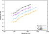 |
Fig. B.1. UV-optical-NIR SEDs between 0.03 and 0.5 days. The Galactic 2175 Å absorption feature is clearly visible in the uvm2-band. |
Across all cases, extinction remains negligible within measurement uncertainties, with a modest preference for the LMC model over the MW model.
Appendix C: The high-velocity component
In section 4.6 we find that the high-velocity, Fe-rich outer ejecta component that fits early spectra produces clearly incorrect spectral features at later epochs. Here we note that this problem is essentially independent from the ejecta composition and density in the inner region; it is the existence of the Fe-rich high-velocity component inferred from the earliest phase-spectra that produces too much absorption even in the later epochs, irrespective of the nature of the input radiation that irradiates the outer region. We have varied both the inner and outer structure and composition in several ways, but have not found a solution that can explain the early and late-time spectra simultaneously. As an example, Fig. C.2 shows the synthetic spectra for a model in which X(56Ni) and X(58Ni) in the outer, high-velocity (> 20, 000 km s−1) component are decreased by a factor of 8 from our reference model (i.e., the same one used for the region in 15, 000 − 20, 000 km s−1). While the absorption below ∼4, 000Å is not sufficient on day 6 and 9, the model already shows the clear problems for the spectra on day 18 and 23. Indeed, the density in the outer region obtained for day 6 and 9 is too large even if this is dominated by the C+O material to be compatible to the spectra on day 18 and 23. As yet another exercise for the spectral analysis on day 18 and 23, we have added pure C+O material (plus the progenitor metals) above 20, 000 km s−1 and changed the slope of the density structure as shown by the dashed line in Fig. 8. We consider this to be an upper limit necessary to not produce too strong high-velocity O I and NIR Ca II, and in fact it is below the one inferred from the spectral analysis on days 6 and 9.
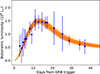 |
Fig. C.1. Monte Carlo Markov Chain fit to the bolometric light curve of SN 2018fip, obtained from our g′r′i′z′J photometry, using the radioactive-heating mode (Arnett 1982). |
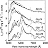 |
Fig. C.2. Another set of the spectral models that do not fit to the observed spectra. The solid curves show the synthesised spectra for the model in which the mass fractions of 56Ni and 58Ni are decreased by a factor of eight as compared to the reference model. The dashed curves adopt a pure C+O composition (plus the progenitor metals) for the high-velocity component. The grey lines show the observed spectra (see the caption of Fig. 7 for details). |
Reference stars for GROND and X-shooter photometry.
Reference stars used for MASTER photometry.
Observations of the afterglow of GRB 180728A.
All Tables
All Figures
|
Fig. 1. Image of the optical afterglow of GRB 180728A obtained in the r-band with the X-shooter acquisition camera on 28 July 2018, 0.23 days after the burst trigger. We highlight the position of the afterglow (indicated as “AG”) and of the nearby star, together with their projected distance. The rectangle shows the X-shooter slit with a position angle of 118.1 deg, which we selected to cover both the afterglow and the nearby star starting with the fourth observation at 6.26 days. The green contours indicate equal count levels. |
| In the text | |
|
Fig. 2. GRB 180728A (red) in the Ep, i − Eγ, iso plane. The GRBs with an associated SN are highlighted in green; outliers are in blue. Dot-dashed lines indicate the ±2σ region. The GRB data are from Amati et al. (2019). |
| In the text | |
|
Fig. 3. Fit to the light curve and supernova of GRB 180728A. Magnitudes are in the AB system and corrected for Galactic foreground extinction, and time is in the observer frame. For reasons of clarity, light curves in each filter are offset by the magnitude values noted in the legend. Starting at ≈300 s, the light curve in all bands except for H and K is fitted with a broken power law plus individual SN component. The dashed line for the white filter is an extrapolation because the points at > 4 days were not fitted. See text for details. |
| In the text | |
|
Fig. 4. X-ray to optical SED at 0.03, 0.1, 0.24 and 1.5 days. The last two epochs are well modelled by a joint-fit with a single power law with spectral slope β ∼ 0.7. In the first two epochs, the optical data have a slightly shallower spectral slope, βopt ∼ 0.6, while the X-ray data do not and require a break that moves from 2.1 to 2.6 keV (with βX = βopt + 0.5). The solid line is the unextinguished and unabsorbed model. The dashed line represents the extinguished and absorbed model, dominated by the Galactic foreground extinction in the optical/NIR bands and absorption in the X-rays. |
| In the text | |
|
Fig. 5. Swift/XRT and optical light curves (MASTER CR band, X-shooter, GROND r′). Note that the optical data of the transient were obtained via image subtraction after 0.2 days, and therefore the contribution of the host is also subtracted. We highlight in cyan the epochs used in the optical-to-XRT SED fitting. Vertical lines highlight epochs with spectroscopic coverage. The dotted lines are the best fit of the optical light curve obtained in Section 4.2, which we have also normalised to the X-rays for data after 5 ks, i.e., excluding the first Swift orbit, which clearly shows that these early data are offset from the fit (see Sect. 4.3). |
| In the text | |
|
Fig. 6. Evolution of the spectra of SN 2018fip in the rest-frame. The absorption features marked in the image refer to the spectrum obtained about 5 days after the peak (day 18). Phases are in the observer frame. |
| In the text | |
|
Fig. 7. Synthesised spectra as compared with those of SN 2018fip. Solid black lines represent the reference model spectra. The dashed black lines (on days 18 and 23) show the synthesised spectra with the high-velocity component included in the spectral synthesis calculations, demonstrating that this component is not present at late epochs. The observed spectra are shown with grey lines. The same constant in flux has been added for the model and data as an offset for presentation purposes (3.6, 2.0, 0.8, and 0.0 for day 6, 9, 18 and 23, respectively). |
| In the text | |
|
Fig. 8. Input density structure for the reference spectral model (solid black lines): the inner lower-velocity component for the spectra on day 18 and 23 (SN 2018fip) and the outer high-velocity component for day six and nine (SN 2018fip-HV). The dashed black line shows the upper limit set by the spectral synthesis analyses on days 18 and 23 (see the main text). The density structures derived for GRB-SNe 2017iuk (Izzo et al. 2019) and 1998bw (Iwamoto et al. 1998) are shown by solid grey and dashed grey lines, respectively. |
| In the text | |
|
Fig. 9. Photospheric velocity used in the reference model (points). The two solid curves show the expected evolution of the photospheric velocity calculated for the reference density structure adopting a constant opacity of 0.03 or 0.6 cm2 g−1. In TARDIS spectral synthesis simulations, the input photospheric velocity is varied as a parameter within the range between the two lines shown here (see Sect. 4.6). |
| In the text | |
|
Fig. 10. RGB-colour image of the host galaxy of GRB 180728A, obtained from i′,r′ g′ images. Bluer regions correspond primarily to g′-band emission. The top panels show the individual g′ r′ i′ z′ GROND imaging. The nearby star (red circle) was removed using a point spread function model, although some residual is left. The magenta circle shows the position of the afterglow/SN. The dashed circle has a radius of 1 |
| In the text | |
|
Fig. 11. Zoom-in on the Hα line and [N II] region of the VLT/X-shooter spectrum of the host galaxy in units of 10−17 erg s−1 cm−2 Å−1. The detected emission lines are marked. A fit of the lines and of the continuum is shown in red. In grey is the error on the spectrum. |
| In the text | |
|
Fig. 12. GROND g′ r′ i′ z′ and VISTA J-band photometry of the host galaxy of GRB 180728A with Cigale (Section 4.7). The best model (solid line) is shown together with the relative residuals. Photometric measurements are marked by violet empty circles. |
| In the text | |
|
Fig. 13. Afterglows of GRBs, all transformed to the z = 1 system following the method of Kann et al. (2006). We highlight (in red) the afterglow of GRB 180728A, which is seen to be among the faintest known in the context of luminosity. We also mark with thick dark grey lines other GRBs at z < 0.5 that are associated with SNe (the SN emission has been subtracted in this plot). |
| In the text | |
|
Fig. 14. X-ray light curve of GRB 180728A in the context of the X-ray afterglows of 473 Swift GRBs with known redshifts (until February 2024). For comparison, we overlay the light curves of Swift GRBs with spectroscopically confirmed SNe and divide the sample into six SN-GRBs with Eγ, iso < 1051 and nine SN-GRBs with Eγ, iso > 1051 erg. The colour table on the right side translates a grey shade at a given luminosity and time into a fraction of bursts. |
| In the text | |
|
Fig. 15. Schematic of the ejecta structure, showing a combination of the 56Ni-rich high-velocity component confined in a narrow solid angle and the slower quasi-spherical ejecta. The black line shows the photosphere at: i) 6 days, when it includes the high-velocity high-velocity component, and ii) at 18 days, when the photosphere recedes in the inner ejecta. |
| In the text | |
|
Fig. 16. Quasi-bolometric light curve of SN 2018fip compared to those of 13 well-observed GRB-SNe, with low-order spline fits shown for each. Most of the comparison light curves, especially for GRB-SNe observed before 2015, are adopted from the compilation by Cano et al. (2017b), which incorporates data from multiple earlier studies cited therein. Additional events were included from more recent works by Cano et al. (2017a), Izzo et al. (2019), Melandri et al. (2019, 2022), Kumar et al. (2022, 2024). |
| In the text | |
|
Fig. 17. Top: Luminosity–stretch diagram colour-coded by Eγ, iso. The dashed line is the best fit from (Klose et al. 2019). Bottom:Ek, SN – Eγ, iso plane, colour-coded by T90. Data are from (Cano et al. 2017b) and have been updated with recent results (Klose et al. 2019; Dainotti et al. 2022; Kann et al. 2024a; Dong et al. 2025). For SN 2018fip, the error on Ek, SN obtained via the Arnett modelling extends up to the one obtained by the spectral modelling and spherical approximation. |
| In the text | |
|
Fig. 18. Distribution of the GRB efficiency ξ% following the approach described in Lü et al. (2018). We highlight GRBs 180728A/SN 2018fip and 111209A/SN 2011kl, which are discussed in the text. |
| In the text | |
|
Fig. B.1. UV-optical-NIR SEDs between 0.03 and 0.5 days. The Galactic 2175 Å absorption feature is clearly visible in the uvm2-band. |
| In the text | |
|
Fig. C.1. Monte Carlo Markov Chain fit to the bolometric light curve of SN 2018fip, obtained from our g′r′i′z′J photometry, using the radioactive-heating mode (Arnett 1982). |
| In the text | |
|
Fig. C.2. Another set of the spectral models that do not fit to the observed spectra. The solid curves show the synthesised spectra for the model in which the mass fractions of 56Ni and 58Ni are decreased by a factor of eight as compared to the reference model. The dashed curves adopt a pure C+O composition (plus the progenitor metals) for the high-velocity component. The grey lines show the observed spectra (see the caption of Fig. 7 for details). |
| In the text | |
Current usage metrics show cumulative count of Article Views (full-text article views including HTML views, PDF and ePub downloads, according to the available data) and Abstracts Views on Vision4Press platform.
Data correspond to usage on the plateform after 2015. The current usage metrics is available 48-96 hours after online publication and is updated daily on week days.
Initial download of the metrics may take a while.