| Issue |
A&A
Volume 708, April 2026
|
|
|---|---|---|
| Article Number | A219 | |
| Number of page(s) | 23 | |
| Section | Cosmology (including clusters of galaxies) | |
| DOI | https://doi.org/10.1051/0004-6361/202558368 | |
| Published online | 08 April 2026 | |
The DESI DR1 peculiar velocity survey: Growth rate measurements from the galaxy power spectrum
1
Aix-Marseille University, CNRS/IN2P3, CPPM, Marseille 13288, France
2
Centre for Astrophysics & Supercomputing, Swinburne University of Technology, P.O. Box 218 Hawthorn, VIC 3122, Australia
3
School of Mathematics and Physics, University of Queensland, Brisbane, QLD 4072, Australia
4
Korea Astronomy and Space Science Institute, 776, Daedeokdae-ro, Yuseong-gu, Daejeon, 34055, Republic of Korea
5
University of Science and Technology, 217 Gajeong-ro, Yuseong-gu, Daejeon, 34113, Republic of Korea
6
Steward Observatory, University of Arizona, 933 N. Cherry Avenue, Tucson, AZ 85721, USA
7
Department of Physics, Carnegie Mellon University, 5000 Forbes Avenue, Pittsburgh, PA 15213, USA
8
Lawrence Berkeley National Laboratory, 1 Cyclotron Road, Berkeley, CA 94720, USA
9
Department of Physics, Boston University, 590 Commonwealth Avenue, Boston, MA 02215, USA
10
Dipartimento di Fisica “Aldo Pontremoli”, Università degli Studi di Milano, Via Celoria 16, I-20133 Milano, Italy
11
INAF-Osservatorio Astronomico di Brera, Via Brera 28, 20122 Milano, Italy
12
Department of Physics & Astronomy, University College London, Gower Street, London WC1E 6BT, UK
13
Department of Physics & Astronomy, University of Rochester, 206 Bausch and Lomb Hall, P.O. Box 270171 Rochester, NY 14627-0171, USA
14
Instituto de Física, Universidad Nacional Autónoma de México, Circuito de la Investigación Científica, Ciudad Universitaria, Cd. de México C. P. 04510, Mexico
15
University of California, Berkeley, 110 Sproul Hall #5800 Berkeley, CA 94720, USA
16
Institut de Física d’Altes Energies (IFAE), The Barcelona Institute of Science and Technology, Edifici Cn, Campus UAB, 08193 Bellaterra (Barcelona), Spain
17
Departamento de Física, Universidad de los Andes, Cra. 1 No. 18A-10, Edificio Ip, CP 111711 Bogotá, Colombia
18
Observatorio Astronómico, Universidad de los Andes, Cra. 1 No. 18A-10, Edificio H, CP 111711 Bogotá, Colombia
19
Institut d’Estudis Espacials de Catalunya (IEEC), c/ Esteve Terradas 1, Edifici RDIT, Campus PMT-UPC, 08860 Castelldefels, Spain
20
Institute of Cosmology and Gravitation, University of Portsmouth, Dennis Sciama Building, Portsmouth PO1 3FX, UK
21
Institute of Space Sciences, ICE-CSIC, Campus UAB, Carrer de Can Magrans s/n, 08913 Bellaterra, Barcelona, Spain
22
University of Virginia, Department of Astronomy, Charlottesville, VA 22904, USA
23
Fermi National Accelerator Laboratory, PO Box 500 Batavia, IL 60510, USA
24
Institut d’Astrophysique de Paris. 98 bis boulevard Arago, 75014 Paris, France
25
IRFU, CEA, Université Paris-Saclay, F-91191 Gif-sur-Yvette, France
26
Center for Cosmology and AstroParticle Physics, The Ohio State University, 191 West Woodruff Avenue, Columbus, OH 43210, USA
27
Department of Physics, The Ohio State University, 191 West Woodruff Avenue, Columbus, OH 43210, USA
28
The Ohio State University, Columbus 43210, OH, USA
29
Department of Physics, University of Michigan, 450 Church Street, Ann Arbor, MI 48109, USA
30
University of Michigan, 500 S. State Street, Ann Arbor, MI 48109, USA
31
Department of Physics, The University of Texas at Dallas, 800 W. Campbell Rd., Richardson, TX 75080, USA
32
NSF NOIRLab, 950 N. Cherry Ave., Tucson, AZ 85719, USA
33
Department of Physics and Astronomy, University of California, Irvine 92697, USA
34
Sorbonne Université, CNRS/IN2P3, Laboratoire de Physique Nucléaire et de Hautes Energies (LPNHE), FR-75005 Paris, France
35
Departament de Física, Serra Húnter, Universitat Autònoma de Barcelona, 08193 Bellaterra (Barcelona), Spain
36
Institució Catalana de Recerca i Estudis Avançats, Passeig de Lluís Companys, 23, 08010 Barcelona, Spain
37
Department of Physics and Astronomy, Siena University, 515 Loudon Road, Loudonville, NY 12211, USA
38
Instituto de Física, Universidad Nacional Autónoma de México, Circuito de la Investigación Científica, Ciudad Universitaria, Cd. de México C. P. 04510, Mexico
39
Department of Physics and Astronomy, University of Waterloo, 200 University Ave W, Waterloo, ON N2L 3G1, Canada
40
Perimeter Institute for Theoretical Physics, 31 Caroline St. North, Waterloo, ON N2L 2Y5, Canada
41
Waterloo Centre for Astrophysics, University of Waterloo, 200 University Ave W, Waterloo, ON N2L 3G1, Canada
42
Space Sciences Laboratory, University of California, Berkeley, 7 Gauss Way, Berkeley, CA 94720, USA
43
Instituto de Astrofísica de Andalucía (CSIC), Glorieta de la Astronomía, s/n, E-18008 Granada, Spain
44
Departament de Física, EEBE, Universitat Politècnica de Catalunya, c/Eduard Maristany 10, 08930 Barcelona, Spain
45
Department of Physics and Astronomy, Sejong University, 209 Neungdong-ro, Gwangjin-gu, Seoul, 05006, Republic of Korea
46
CIEMAT, Avenida Complutense 40, E-28040 Madrid, Spain
47
Department of Physics & Astronomy, Ohio University, 139 University Terrace, Athens, OH 45701, USA
48
National Astronomical Observatories, Chinese Academy of Sciences, A20 Datun Road, Chaoyang District, Beijing 100101, P.R. China
★ Corresponding author: This email address is being protected from spambots. You need JavaScript enabled to view it.
Received:
2
December
2025
Accepted:
12
February
2026
Abstract
The large-scale structure of the Universe and its evolution encapsulate a wealth of cosmological information. A powerful means of unlocking this knowledge lies in measuring the auto-power spectrum and/or the cross-power spectrum of the galaxy density and momentum fields, followed by the estimation of cosmological parameters based on these spectrum measurements. In this study, we generalize the cross-power spectrum model to accommodate scenarios in which the density and momentum fields are derived from distinct galaxy surveys. The growth rate of the large-scale structures of the Universe, commonly represented as fσ8, was extracted by jointly fitting the monopole and quadrupole moments of the auto-density power spectrum, the monopole of the auto-momentum power spectrum, and the dipole of the cross-power spectrum. Our estimators, theoretical models, and parameter-fitting framework were tested using mocks, confirming their robustness and accuracy in retrieving the fiducial growth rate from simulation. These techniques were then applied to analyse the power spectrum of the DESI Bright Galaxy Survey and Peculiar Velocity Survey. The fit result of the growth rate is fσ8 = 0.440+0.080−0.096 at effective redshift zeff = 0.07. By synthesizing the fitting outcomes from correlation functions, maximum likelihood estimation, and the power spectrum, a consensus value is yielded of fσ8(zeff = 0.07) = 0.450+0.055−0.055, and correspondingly we obtain γ = 0.580+0.110−0.110, Ωm = 0.301+0.011−0.011, and σ8 = 0.834+0.032−0.032. The measured fσ8 and γ are consistent with the prediction of the Λ cold dark matter model and general relativity.
Key words: cosmological parameters / large-scale structure of Universe
© The Authors 2026
 Open Access article, published by EDP Sciences, under the terms of the Creative Commons Attribution License (https://creativecommons.org/licenses/by/4.0), which permits unrestricted use, distribution, and reproduction in any medium, provided the original work is properly cited.
This article is published in open access under the Subscribe to Open model. This email address is being protected from spambots. You need JavaScript enabled to view it. to support open access publication.
1. Introduction
One of the most profound scientific pursuits in cosmology is to unravel the evolutionary processes that have shaped the large-scale structures of our Universe. Galaxies exhibit peculiar motions – superimposed on their Hubble recession velocities – due to gravitational fluctuations arising from local variations in the matter density field. These peculiar velocities serve as a crucial observational probe, offering deep insights into the underlying dark matter distribution and the dynamic history of cosmic expansion and structure formation. Consequently, they have garnered growing interest as an essential diagnostic tool for assessing the accuracy and predictive power of cosmological models.
An approach to assess the cosmological models involves measuring the low-order kinematic moments of the cosmic flow field based on the radial components of galaxies’ peculiar velocities, and subsequently comparing these estimates with the predictions of the cosmological models (Kaiser 1988; Strauss & Willick 1995; Feldman et al. 2010; Scrimgeour et al. 2016; Zhang et al. 2017; Qin et al. 2018, 2019b; Qin 2021; Qin et al. 2021; Whitford et al. 2023). However, due to the significant cosmic variance inherent in low-redshift velocity surveys, the constraints imposed on cosmological models through this method are typically not tight.
An alternative approach involves estimating cosmological parameters and subsequently comparing them with predictions of cosmological models. In the field of cosmology, researchers commonly aim to investigate the rate at which large-scale structures evolve, as well as the ratio between galaxy density and dark matter density. The former quantity is associated with the structure linear growth rate, f, while the latter relates to the galaxy biasing parameter, b. Furthermore, in practical applications, normalized parameters fσ8 and bσ8 have attracted attention as measurable quantities. σ8 refers to the root mean square of mass density fluctuations within spheres of 8 Mpc h−1. Various methodologies have been proposed in prior studies to extract these parameters from galaxy survey data (Ishak 2019; Ishak et al. 2025).
One technique involves the reconstruction of the cosmological density and velocity fields (Nusser et al. 1991; Kitaura et al. 2012; Wang et al. 2012), or the cosmography of the local Universe (Courtois et al. 2013; Dupuy & Courtois 2023). The parameters fσ8 and bσ8 can be estimated by comparing the observed peculiar velocities of galaxies with the reconstructed velocity field (Carrick et al. 2015; Said et al. 2020; Boruah et al. 2022). However, systematic errors associated with this method are difficult to quantify, and previous studies have indicated that the errors tend to be underestimated (Turner & Blake 2023; Blake & Turner 2024). Recently, artificial intelligence techniques have increasingly been applied to field reconstruction (Hong et al. 2021; Qin et al. 2023a; Wu et al. 2023), offering novel opportunities in this research area. Moreover, since the covariance matrix of the density and velocity fields can be formulated in terms of fσ8 and bσ8, these parameters can alternatively be estimated by maximizing the likelihood function under the assumption of a Gaussian distribution (Johnson et al. 2014; Adams & Blake 2017; Lai et al. 2023; Carreres et al. 2023; Rocher et al. 2023; Ravoux et al. 2025). However, this method remains computationally demanding. Another commonly used approach is the two-point statistic method, which has played a significant role in cosmology over the past decades. Based on this method, fσ8 and bσ8 can be derived from the galaxy two-point correlation functions, the velocity-correlation functions, and the galaxy-velocity cross-correlation functions (Gorski et al. 1989; Howlett et al. 2015; Dupuy et al. 2019; Wang et al. 2018; Turner et al. 2021, 2023; Qin et al. 2022, 2023b; Lyall et al. 2023). Nevertheless, these approaches tend to be computationally intensive too.
Instead of studying the two-point correlations in configuration space, we can also analyse them in Fourier space, i.e. analysing the so-called power spectrum. The concept of the cosmological power spectrum was first introduced by Kaiser (1987). The first measurement of the (galaxy) density power spectrum was carried out by Kaiser & Peacock (1991). The methodology for estimating the density power spectrum was later refined by Feldman et al. (1994), forming the standard approach widely used today. In addition to these foundational contributions, Yamamoto et al. (2006) and Bianchi et al. (2015) further developed estimators for the multipoles of the density power spectrum.
However, the linear growth rate of the structure, fσ8 is only primarily sensitive to higher-order components of the density power spectrum, resulting in relatively weak constraints when inferred from this method alone. To improve the estimation of fσ8, the momentum power spectrum – initially explored in Park (2000) – has recently gained widespread use in cosmology. Howlett (2019, hereafter Paper I) adapted the momentum power spectrum method to be implemented in a manner analogous to the conventional density power spectrum approach. Qin et al. (2019a, hereafter Paper II) successfully applied the momentum power spectrum to constrain fσ8 using data from the combined 6dFGS peculiar velocity survey (6dFGSv; Campbell et al. 2014) and 2MASS Tully-Fisher (2MTF; Hong et al. 2019) survey. Building upon their research, Qin et al. (2025, hereafter Paper III) advanced the existing methodology by extending it to the cross-power spectrum of density and momentum fields – both derived from a unified survey catalogue. Their work achieved a successful estimation of fσ8 through the peculiar velocity data from the Sloan Digital Sky Survey peculiar velocity catalogue (SDSSv; Howlett et al. 2022). This paper marks the fourth in the ongoing series. Herein, we further refine and expand our analytical framework to model and measure the cross-power spectrum in more complex cases, where the density and momentum fields are drawn from distinct galaxy survey catalogues, each exhibiting unique survey geometries, selection criteria, and sample characteristics. Additional studies employing the momentum power spectrum include those by Park & Park (2006), Appleby et al. (2023) and Shi et al. (2024).
We constrained fσ8 using Data Release 1 (DR1) from the Bright Galaxy Survey (BGS; Hahn et al. 2023) and Peculiar Velocity Survey (DESI-PV; Carr et al. 2025; Ross et al. 2025; Douglass et al. 2025) of the Dark Energy Spectroscopic Instrument (DESI; DESI Collaboration 2025a,b). The DESI-PV DR1 stands as the largest peculiar velocity survey ever assembled to date. This paper forms part of a comprehensive series of results from DESI-PV DR1 (Turner et al. 2025; Lai et al. 2025; Ross et al. 2025; Douglass et al. 2025; Bautista et al. 2025; Carr et al. 2025; Nguyen et al. 2025).
This paper is organized as follows. Section 2 presents the data and mocks employed for measuring the power spectrum. Section 3 introduces the estimators utilized to compute the power spectrum. Section 4 delves into the theoretical models of the power spectrum. In Sect. 5 we outline the fitting methodologies and validate our estimators and models through extensive testing on mocks. Section 6 showcases the final parameter fitting results derived from the survey data. In Sect. 7 we discuss the parameter constraints in light of predictions and fits from other data sets. Lastly, Sect. 8 offers a comprehensive conclusion summarizing the key findings of the study.
In this paper, we adopt the AbacusSummit (Maksimova et al. 2021) cosmological parameters1ns = 0.96490, As = 2.101198 × 10⁻⁹, Ωm = 0.315192, Ωbh2 = 0.02237, Ωch2 = 0.12000, σ8 = 0.8113545, and H0 = 100 h km s−1 Mpc−1, where h = 0.67360. We adopt a flat Λ cold dark matter (ΛCDM) fiducial cosmological model.
2. Data and mocks
2.1. The Dark Energy Spectroscopic Instrument
Located at the Kitt Peak National Observatory in Arizona, USA, the Dark Energy Spectroscopic Instrument is a multi-fibre spectrograph mounted on the 4-meter Mayall Telescope, designed to explore the large-scale structure of the Universe and the expansion history of the Universe (Levi et al. 2013; DESI Collaboration 2016a,b, 2022; Miller et al. 2024; Poppett et al. 2024). The DESI focal plane spans 8 square degrees and is equipped with 5000 optical fibres, each of which can be positioned onto individual targets within an observational field using robotic positioners (Silber et al. 2023). The spectrographs span the near-ultraviolet to near-infrared spectrum (3600–9800 Å), delivering a spectral resolution that ascends from 2000 in the blue camera to 5000 in the red camera. The observing strategy is detailed in Guy et al. (2023) and Schlafly et al. (2023). Following its Early Data Release (EDR; DESI Collaboration 2024a,b), the survey has now progressed to DR1 (DESI Collaboration 2025a,c). For this study, the galaxy sample was drawn from the DESI DR1 catalogue. We used the DESI DR1 large-scale structure catalogue2 (DESI Collaboration 2025e).
2.1.1. The BGS data
The Bright Galaxy Survey (BGS; Hahn et al. 2023) Bright sample has undergone refinement by Turner et al. (2025), who introduced tailored selection criteria to enhance its suitability for analyses involving peculiar velocities. The final BGS data catalogue employed in our study encompasses a total of 415 523 galaxies, with an r-band absolute magnitude threshold set at −17.7. The sky distribution of these galaxies is illustrated by the black dots in Fig. 1. Furthermore, the redshifts of these galaxies, measured in the CMB frame, span the range from z = 0.01 to z = 0.1, as is depicted by the black bars in Fig. 2. The galaxy mean number density,  , is shown in the top left panel of Fig. 3. The calculation of
  is detailed in Bautista et al. (2025). In this paper, the density field was derived from the BGS catalogue.
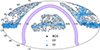 |
Fig. 1. Sky coverage in equatorial co-ordinates of the galaxies analysed within this study. The black dots delineate the sky distribution of BGS galaxies, the grey dots represent that of FP galaxies, and the blue dots illustrate the distribution of TF galaxies. The purple band signifies the galactic plane. |
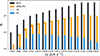 |
Fig. 2. Redshift distribution of the galaxies employed in this paper. The y axis is presented on logarithmic scales to enhance the clarity of the data. The black bars depict the redshift distribution of the BGS galaxies, the grey bars delineate the redshift distribution of FP galaxies, and the blue bars illustrate the redshift distribution of TF galaxies. Additionally, the yellow bars represent the redshift distribution of the entire DESI-PV sample, which constitutes a combination of FP and TF galaxies. |
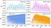 |
Fig. 3. Galaxy mean number density, denoted as |

2.1.2. The DESI-PV data
Due to the peculiar motions of galaxies, the apparent distance of a galaxy, denoted as dz, deviates from its true comoving distance, dh. This discrepancy is measurable and can be quantified through the logarithmic distance ratio, defined as  . It can be converted to the line-of-sight peculiar velocity using the velocity estimator Eq. (A.1). Within the DESI-PV survey, two distinct populations of galaxies are observed: spiral galaxies, also known as late-type galaxies, and elliptical galaxies, referred to as early-type galaxies. The η for late-type galaxies is derived from the Tully-Fisher (TF; Tully & Fisher 1977) relation, whereas for early-type galaxies it is inferred from the fundamental plane (FP; Djorgovski & Davis 1987, Dressler et al. 1987) relation. In DESI-PV, the TF sample (Douglass et al. 2025) comprises a total of 6,806 late-type galaxies. The sky distribution of these galaxies is illustrated by the blue dots in Fig. 1. Furthermore, the redshifts of these galaxies span the range from z = 0.015 to z = 0.1, as depicted by the blue bars in Fig. 2. In contrast, the FP sample (Ross et al. 2025) consists of 73 822 early-type galaxies. Their sky distribution is marked by grey dots in Fig. 1, and their redshifts span the interval from z = 0.01 to z = 0.1, as is shown in the grey bars of Fig. 2.
The DESI-PV catalogue is a combination of the TF sample and the FP sample. The zero-point calibration bridging these two datasets has been rigorously investigated by Carr et al. (2025), ensuring a physical alignment. The redshift distribution of this combined sample is illustrated by the yellow bars in Fig. 2. Meanwhile, the galaxy mean number density,  , is depicted in the top right panel of Fig. 3. In this study, the momentum field was constructed from the DESI-PV catalogue. In accordance with the reasoning articulated in Turner et al. (2025), we imposed a redshift cut of zcut = 0.05 on the TF galaxies when measuring the power spectrum – excluding those galaxies lying beyond this threshold – to mitigate systematic biases inherent in the TF velocity measurements. This identical redshift cut was consistently applied across both mocks and random catalogues, ensuring coherence and comparability throughout the analysis. Following Turner et al. (2025), a 4σ-clipping was applied to the measured η values of the DESI-PV data too.
2.2. Mocks
A considerable number of mocks is indispensable for validating the algorithm and accurately estimating the uncertainties in the power spectrum and associated parameters. Bautista et al. (2025) offers a comprehensive set of 675 BGS mocks, meticulously designed to mirror the characteristics of the BGS data. In parallel, 675 FP mocks have been constructed to emulate the FP data, alongside 675 TF mocks tailored to align with the TF data. Each set of BGS, FP, and TF mocks shares the same observer, resulting in a total of 675 mock sets. These mocks were derived from the AbacusSummit simulation, and the fiducial value of fσ8 for these mocks is 0.466 at an effective redshift of z = 0.2.
The FP and TF mocks were generated with the specific aim of replicating the selection function and survey geometry, the FP relation, the TF relation, and the galaxy clustering observed in the FP and TF data, respectively. The DESI-PV mocks were formed by combining the TF and FP mocks. The galaxy mean number density,  , of DESI-PV mocks is illustrated in the bottom right panel of Fig. 3. The galaxy mean number density,
  , of BGS mocks is illustrated in the bottom left panel of Fig. 3.
2.3. The random catalogues
The random catalogues for both the data and mocks are also supplied by Bautista et al. (2025). In order to precisely extract cosmological parameters from the power spectrum, it is imperative to appropriately account for the survey geometry of both BGS and DESI-PV. Employing fast Fourier transforms to measure the power spectrum in the context of a non-periodic and incomplete survey geometry leads to a convolution of the true power spectrum with the survey’s window function. To address this, the random catalogue was employed to estimate the window function, thereby enabling the application of an equivalent convolution to our theoretical model during the data fitting process. The random catalogues for FP and TF were generated independently, with the objective of more faithfully replicating the distinct observational features of the TF and FP surveys, respectively. The random catalogue for DESI-PV was constructed by combining the random catalogues of TF and FP.
3. The estimation of the power spectrum
3.1. The field functions
In this paper, we investigate the redshift-space power spectrum of galaxies, encompassing both the auto-power spectrum and cross-power spectrum of the galaxy density and momentum fields. The density field was derived from the BGS catalogue, whereas the momentum field was obtained from the DESI-PV catalogue. Within our paper series, the density (contrast) field is defined by
 (1)
(1)
where ρ(r) is the mass density at position r = [rx, ry, rz], and  represents the average mass density of the Universe. The line-of-sight momentum field is defined by
![Mathematical equation: $$ \begin{aligned} p(\mathbf{r})\equiv [1+\delta (\mathbf{r})]v(\mathbf{r}),\end{aligned} $$](/articles/aa/full_html/2026/04/aa58368-25/aa58368-25-eq15.gif) (2)
(2)
with v(r) denoting the line-of-sight peculiar velocity at position r. The auto-density power spectrum, Pδ, the auto-momentum power spectrum, Pp, and the cross-power spectrum of the density and momentum fields, Pδp, were originally formulated as two-point correlations of δ and/or p in Fourier space, as expressed in
 (3)
(3)
 (4)
(4)
 (5)
(5)
respectively, where δD(k − k′) indicates the Dirac δ function and ‘*’ denotes the complex conjugate. k is the wave vector.
We favour the momentum power spectrum over the velocity power spectrum because, in principle, the velocity field is a continuous entity defined everywhere in space, even in regions devoid of galaxies. However, our measurements are limited to locations where galaxies (and thus mass) are present, effectively yielding a mass-weighted or momentum-based power spectrum. In regions devoid of galaxies, we record zero velocity not because the velocity is truly zero, but due to the absence of tracers. Additionally, the momentum power spectrum retains the same fundamental information as the velocity power spectrum, and with additional non-linear contributions introduced by the (1 + δ) term that are incorporated into the theoretical modelling.
Following the methodology outlined in Feldman et al. (1994), which constitutes the standard approach widely adopted today, the estimator for the density field is presented in
![Mathematical equation: $$ \begin{aligned} F^{\delta }(\mathbf{r})\equiv \frac{w_{\delta }(\mathbf{r})\left[ n_{\delta }(\mathbf{r})-\alpha n_s(\mathbf{r}) \right]}{A_{\delta }}. \end{aligned} $$](/articles/aa/full_html/2026/04/aa58368-25/aa58368-25-eq19.gif) (6)
(6)
In this formulation wδ(r), nδ(r) and ns(r) represent the weight factor, the number density of galaxies, and the number density of random points at position r. The number of random points is α times greater than the number of galaxies. Aδ serves as the normalization factor, defined by
 (7)
(7)
which ensures that the amplitude of the measured power aligns with it in a Universe unaffected by survey selection effects. The computation of the mean galaxy number density,  , at position r is detailed in Bautista et al. (2025) or see Fig. 3. As is indicated in Eq. (6), to estimate the density field it is necessary to subtract the random catalogue. This is because we measure the density contrast field, δ, which can only be accomplished if we possess knowledge of, and are able to subtract, the mean number of galaxies within each grid cell, estimated from randoms of that cell.
Similarly, following the derivation in Paper I, the estimator for the momentum field is given by
 (8)
(8)
where wp(r) and np(r) denote the weight factor and the number density of galaxies at position r, respectively. Ap functions as the normalization factor, defined by
 (9)
(9)
which again adjusts the amplitude of the measured power to conform with it in an idealized Universe without survey selection biases. The computation of the mean galaxy number density,  , at position r is also detailed in Bautista et al. (2025) (or see Fig. 3). Notably, no random catalogue is subtracted when estimating the momentum field. This is because that the mean velocity at any spatial point is inherently zero; consequently, subtracting a random catalogue during the construction of the momentum field would be equivalent to subtracting zero.
In this paper, we define the Fourier transform of the field functions presented in Eqs. (6) and (8) through the following formulation:
 (10)
(10)
and inversely,
 (11)
(11)
3.2. The estimators of the power spectrum multipoles
The observed redshift of a galaxy comprises two dominant contributions: the Hubble recessional redshift resulting from the cosmic expansion, and the peculiar velocity redshift arising from localized gravitational influences. Consequently, the inferred position of a galaxy based on its observed redshift does not represent its true comoving position; instead, it reveals a distorted position that is referred to as the ‘redshift-space position’. This phenomenon is widely recognized as redshift-space distortion (RSD).
Redshift-space distortions disrupt the spherical symmetry of the power spectrum with respect to the line of sight. To capture this anisotropic behavior, a prevalent methodology involves decomposing the redshift-space power spectrum, P(k), into a series of Legendre polynomials, Lℓ(μ), i.e.
 (12)
(12)
In this decomposition, the angular dependence of the power spectrum, P(k), is encapsulated within the Legendre polynomials, Lℓ(μ), while the amplitude information of P(k) are encoded in the multipole moments, Pℓ(k), commonly referred to as power spectrum multipoles. Here,  denotes the cosine of the angle between the unit wave vector,
  , and the line-of-sight unit vector,
  .
.
Following the formalism established by Yamamoto et al. (2006) and Paper I, the estimators for the auto-density and auto-momentum power spectrum multipoles are defined by
 (13)
(13)
and
 (14)
(14)
respectively. The indices ‘δ’ and ‘p’ corresponds to the auto-density and auto-momentum power spectrum, respectively. The associated shot-noise contributions are described by
 (15)
(15)
 (16)
(16)
respectively.
As is outlined in Appendix H.1 (or see Paper III), the estimator for the cross-power spectrum multipoles is defined through3
 (17)
(17)
with the corresponding shot-noise term detailed in
 (18)
(18)
In this context, ‘δp’ specifically refers to the density-momentum cross-power spectrum, while ‘Im’ denotes the imaginary part of a complex number. Given that both the time evolution of gravitational interactions and the initial conditions of the Universe remain invariant under the transformation δ → −δ and v → −v, the cross-power spectrum between the density and momentum fields must also exhibit invariance under such transformations. This leads directly to the identity  , which holds exclusively for purely imaginary functions. See Appendix B for more details.
The shot noise observed in the auto-power spectrum originates from the discrete nature of galaxies as tracers of the underlying density and momentum fields. In the case of the cross-power spectrum, shot noise arises due to the potential overlap of galaxies used in the estimation of both the density and momentum fields. This form of noise is proportional to the sample containing fewer objects (Smith 2009).
The expressions for the estimators of auto-power spectrum multipoles have been thoroughly examined by Bianchi et al. (2015). Nevertheless, our formulations of the field function definitions and Fourier transform definition deviate slightly from that of Bianchi et al. (2015). Consequently, below we restate the corresponding expressions for clarity and consistency. For convenience, we adopt the methodological framework proposed by Bianchi et al. (2015) and introduce the following function:
 (19)
(19)
where ℓ = 0, 1, 2, 3, 4, .... Consequently, based on Eq. (13) or Eq. (14), the corresponding even-multipoles of the auto-power spectrum are expressed in (see Appendix H.3 for more discussion)
![Mathematical equation: $$ \begin{aligned} P_0(k) = \frac{1}{V} \int \frac{d\Omega _k}{4\pi }[F(\mathbf{k}) T_0^*(\mathbf{k}) ]-\fancyscript {N}_0 \end{aligned} $$](/articles/aa/full_html/2026/04/aa58368-25/aa58368-25-eq39.gif) (20)
(20)
![Mathematical equation: $$ \begin{aligned} P_2(k) = \frac{5}{2V }\int \frac{d\Omega _k}{4\pi }F(\mathbf{k})\left[ 3T^*_2(\mathbf{k})-T^*_0(\mathbf{k}) \right] \end{aligned} $$](/articles/aa/full_html/2026/04/aa58368-25/aa58368-25-eq40.gif) (21)
(21)
![Mathematical equation: $$ \begin{aligned} P_4(k) = \frac{9}{8V }\int \frac{d\Omega _k}{4\pi }F(\mathbf{k})\left[ 35T^*_4(\mathbf{k})-30T^*_2(\mathbf{k})+3T^*_0(\mathbf{k}) \right] ,\end{aligned} $$](/articles/aa/full_html/2026/04/aa58368-25/aa58368-25-eq41.gif) (22)
(22)
where dΩk denotes the solid angle. See Appendix D for the expressions of T0, T2, and T4. It is important to note that, unlike in Bianchi et al. (2015), the normalization factors Aδ and Ap are inherently incorporated within the field functions in our formulation, and our definition of Fourier transformation diverges from them too. For multipoles with ℓ > 0, the shot noise becomes negligible and can be safely ignored (Blake et al. 2010; Howlett 2019). If ignoring the wide-angle or general relativistic effects, only the even-multipoles of the auto-power spectrum are non-zero (Bianchi et al. 2015; Beutler & Di Dio 2020; Castorina & White 2020).
In this paper, building upon Eq. (17) and Eq. (19), we derive the associated odd-multipoles for the cross-power spectrum, as expressed in
 (23)
(23)
![Mathematical equation: $$ \begin{aligned} P_3(k)&=\frac{7}{2 V}\int \frac{d\Omega _k}{4\pi } \bigg [ 5\times \frac{\mathrm{Im} \{F^p(\mathbf{k}) T^{\delta *}_3(\mathbf{k})-F^{\delta }(\mathbf{k}) T^{p*}_3(\mathbf{k}) \}}{2}\nonumber \\&\qquad -3\times \frac{\mathrm{Im} \{F^p(\mathbf{k}) T^{\delta *}_1(\mathbf{k})-F^{\delta }(\mathbf{k}) T^{p*}_1(\mathbf{k}) \}}{2} \bigg ]. \end{aligned} $$](/articles/aa/full_html/2026/04/aa58368-25/aa58368-25-eq43.gif) (24)
(24)
See Appendix D for the expressions of T1 and T3. For similar reasons, only the odd-multipoles exhibit non-vanishing contributions to the cross-power spectrum, and the influence of shot noise diminishes to a negligible extent for ℓ > 0.
3.3. The FKP weights
In Feldman et al. (1994), the authors introduced a weighting scheme for the density power spectrum aimed at minimizing the fractional variance of its estimation. This method is widely known as the Feldman-Kaiser-Peacock (FKP) weighting scheme and is given by
 (25)
(25)
Building upon this work, Paper I proposed an analogous weighting strategy tailored specifically for the momentum field, given by
 (26)
(26)
where ⟨v2(r)⟩ accounts for both intrinsic scatter and measurement errors associated with peculiar velocity estimates and can be calculated using Eq. (A.3).
The FKP weights were derived under the assumption that the power spectrum follows a Gaussian distribution. However, FKP weights may not represent the optimal choice when the power spectrum is not Gaussian. As is demonstrated in Sect. 6 of Paper I, varying the value of PFKP(k) alters the effective survey depth of the galaxy survey. Different choices of FKP weights influence the trade-off between upweighting higher redshift data – thereby increasing cosmic volume and reducing power spectrum variance – and upweighting nearby objects where velocity measurement errors are smaller. Following Paper I, Paper II, and Paper III, we set  and
and  for the density and momentum fields, respectively, to achieve optimal measurement accuracy.
3.4. Grid correction and Nyquist frequency
To compute the field functions of Eq. (6) and (8) from galaxies, it is necessary to assign the galaxies to a three-dimensional grid. This gridding process effectively convolves the field values with a top-hat window function in each spatial direction, resulting in each Fourier mode being multiplied by a Sinc function. To mitigate this effect, following the methodology outlined in Abate et al. (2008), Johnson et al. (2014), and Adams & Blake (2017), we applied a correction factor by dividing each voxel corresponding to a wave vector of k = [kx, ky, kz] by the following Sinc functions for the Fourier transformed field functions (i.e. F(k) and Tℓ(k)):
 (27)
(27)
where Lx, Ly, and Lz denote the size of the voxel in the x, y, and z directions, respectively. In this study, we constructed the galaxy grid using a voxel size of Lx = Ly = Lz = 2 Mpc h−1 within a cubic box of size L = 800 Mpc h−1 centred on the observer. This configuration provides sufficient spatial coverage to include the galaxies observed in the DESI survey.
Furthermore, we consider only those Fourier modes corresponding to wave numbers, k, that exceed the Nyquist frequency, defined by
 (28)
(28)
This ensures that the sampling rate meets the minimum requirement for an undistorted estimation of the power spectrum.
4. The theoretical model of the power spectrum
4.1. The models of power spectrum
Kaiser (1987) developed a linear model for the density power spectrum, commonly referred to as the Kaiser formula (see Appendix C), which has been extensively utilized over the past few decades. Building upon this foundation, Koda et al. (2014) extended the analysis to the power spectrum of peculiar velocities, and incorporated empirical damping terms into the linear models in order to more accurately account for non-linear motions of galaxies. However, these linear and quasi-linear models are effective only for k < 0.15 h Mpc−1, where measurement errors tend to be larger.
To more effectively capture non-linear effects and extend the analysis into regions with smaller measurement errors, we employed one-loop perturbation theory models for the power spectrum in this paper. These redshift-space power spectrum models were initially developed by Vlah et al. (2012, 2013), Okumura et al. (2014) and summarized in Appendix A of Paper I and updated in Sect. 4 of Paper III. Following the theoretical framework outlined in Vlah et al. (2012, 2013) and Paper I, the density power spectrum model is described by
 (29)
(29)
Based on the theoretical formulation presented in Okumura et al. (2014) and Paper I, the momentum power spectrum model is given by
![Mathematical equation: $$ \begin{aligned} P^{p}(k,\mu ) = \frac{[a(z)H(z)]^2}{k^{2}}\big [P_{11}+\mu ^2(2P_{12}+3P_{13}+P_{22})\big ] . \end{aligned} $$](/articles/aa/full_html/2026/04/aa58368-25/aa58368-25-eq51.gif) (30)
(30)
Additionally, the cross-power spectrum model was also derived in Okumura et al. (2014). However, according to Chen et al. (2025, Eq. (D.2) therein), there exist minor inaccuracies in the derivation of the cross-power spectrum expression in Okumura et al. (2014, Eq. (2.19) therein), and consequently in Paper III. In this paper, we derived the corrected version, which is given in
![Mathematical equation: $$ \begin{aligned} P^{\delta p}(k,\mu )&=\frac{a(z)H(z)}{k} \mu \Bigg [P_{01} + P_{02} + P_{11} \nonumber \\&+ \mu ^2\bigg (\frac{3}{2}P_{03} + 2 P_{04} + \frac{3}{2} P_{12} + 2P_{13} + \frac{1}{2}P_{22}\bigg ) \Bigg ]. \end{aligned} $$](/articles/aa/full_html/2026/04/aa58368-25/aa58368-25-eq52.gif) (31)
(31)
Notably, this is the imaginary part of the cross-power spectrum model. The new formulations for Pmn, (m, n = 0, 1, 2, 3, 4) are presented in Sect. 4.2. In the aforementioned equations, the scale factor was determined from
 (32)
(32)
Assuming ΛCDM, the Hubble parameter is given by
 (33)
(33)
where H0, Ωm, and ΩΛ are the Hubble constant, matter density parameter, and dark energy density parameter in the present-day Universe at effective redshift zeff = 0.
The models described in Eq. (29), (30), and (31) represent highly general frameworks, with the sole underlying assumption being the local plane-parallel approximation. These models do not presuppose the ΛCDM paradigm. To derive the ΛCDM-specific models, one simply needs to employ ΛCDM theory in the computation of E(z) (in Eq. (33)), and the growth factor D(a) (in Eq. (44)), as well as the linear matter power spectrum, PL (as was mentioned in Sect. 4.2). However, one is entirely at liberty to utilize alternative theoretical approaches to calculate PL, D(a) and E(z), thereby generating power spectrum models corresponding to other cosmological models.
To obtain the theoretical models for the power spectrum multipoles, one can substitute Eq. (29), (30) and (31) into the following:
 (34)
(34)
which essentially performs a Legendre transformation corresponding to Eq. (12). The aforementioned theoretical models for the power spectrum can be readily converted into models for the galaxy two-point correlation function, the velocity correlation function, and the galaxy-velocity cross-correlation function using the HANKL package4 (Karamanis & Beutler 2021); see Turner et al. (2025) and Appendix C for more discussion. The momentum correlation is equivalent to the velocity correlation in linear scales, as demonstrated by Eq. (2) of Paper I; therefore, the model of the velocity correlation function can be converted from the model of the momentum power spectrum approximately.
4.2. The new loop terms for the cross power spectrum
The loop terms, Pmn, (m, n = 0, 1, 2, 3, 4), in Eq. (29), 30, and 31 were initially formulated by Vlah et al. (2012, 2013), Okumura et al. (2014), Paper I and Paper III. Their models, however, were specifically tailored for situations in which both density and momentum fields originate from the same galaxy survey dataset.
In this paper, we generalize Pmn of cross-power spectrum Eq. (31) to accommodate cases in which the density and momentum fields stem from different surveys with differing observational properties. This generalization implies that the cross-power spectrum Eq. (31) will incorporate multiple biasing parameters. The corresponding new formulations for Pmn (of Eq. (31)) are detailed in the subsequent equations:
 (35)
(35)
 (36)
(36)
 (37)
(37)
 (38)
(38)
 (39)
(39)
where the indices δ and p denote the parameters for density and momentum fields, respectively. The terms P00 in the expression of P04 should be calculated from Eq. (35) of this paper. Following the derivation outlined in Paper III, we arrive at
 (40)
(40)
 (41)
(41)
where P00 and P01 in the above equations should be obtained from Eqs. (35) and (36) of this paper, separately. By following the derivation presented in Paper I, we also obtain
 (42)
(42)
 (43)
(43)
In the above, the P00, P01, and P02 should be derived from Eq. (35), (36), and (40) of this paper, respectively. The term D represents the linear growth factor. Under the assumption of general relativity (GR) and ΛCDM, its analytical expression is given by (Heath 1977; Howlett et al. 2015)
 (44)
(44)
where
 (45)
(45)
and where Dgr, 0 symbolizes the Dgr(a) of the present-day Universe at redshift zeff = 0. E(a) is given in Eq. (33). The terms Imn, Kmn, Kmns, σ3, and σ4 were derived from integrations of the linear matter power spectrum PL, following the approach detailed in Vlah et al. (2012) and Paper I. In this study, we utilized the CAMB5 package (Lewis et al. 2000) to calculate PL(k) assuming ΛCDM, with the resulting PL(k) illustrated in Fig. C.1.
The parameters of the power spectrum models are summarized in Table 1. Within the context of the cross-power spectrum formalism Eq. (31), the fully parameterized model comprises ten parameters. On the other hand, by equating the biasing parameters and velocity dispersion parameters of the density field with those of the momentum field, Eqs. (35) to (43) simplify to the expressions detailed in Appendix A of Paper I. As a result, we obtain the Pmn for the auto-density and auto-momentum power spectrum models (i.e. Eqs. (29) and (30)) conform to the formulations proposed by Paper I, Paper II and Paper III. As was argued in McDonald & Roy (2009), Saito et al. (2014) and Paper I, two higher-order galaxy biasing parameters can be determined from the linear bias using local Lagrangian relations:
 (46)
(46)
Parameters of the power spectrum models.
They can also be set as free parameters when fitting the models to the measurements to gain more flexibility from the models.
Furthermore, setting all of the loop terms, Imn, Kmn, Kmns, σ3, and σ4, to zero, in conjunction with setting the higher-order biasing and velocity dispersion parameters to zero, leads to a reduction in the power spectrum models in Eqs. (29), (30), and (31) to the Kaiser formulas, as is demonstrated in Fig. C.2.
4.3. The window function convolution
In actual astronomical observations, our view is confined to galaxies residing within a limited spatial volume and with a particular sky completeness function. Consequently, the power spectrum measured from galaxy surveys reflects only the characteristics of this restricted volume, rather than representing the entire Universe. However, theoretical formulations of the power spectrum are typically based on the infinitely extended Universe. Therefore, in order to reliably infer cosmological parameters from galaxy surveys, it is crucial to incorporate the impacts of survey geometry and observational completeness when comparing theoretical models with measured power spectrum. This necessitates the application of a convolution operation involving the window function, as formally described by
 (47)
(47)
where the model power spectrum multipoles Pℓ′(k′) (ℓ′ = 0, 1, 2, 3, 4, ...) are concatenated into a single vector, P(k′) = [P0(k′), P1(k′), P2(k′), P3(k′), P4(k′), ...]. The term Pc(k) denotes the convolved model power spectrum multipoles, which serves as the counterpart for direct comparison with the measured power spectrum multipole. The window function convolution matrix, W, is characterized by dimensions (Nℓ × Nk)×(Nℓ′ × Nk′). Specifically, Nk denotes the number of k bins associated with each measured power spectrum multipole, while Nℓ represents the total count of measured power spectrum multipoles. Furthermore, Nk′ indicates the number of k′ values employed in computing each model power spectrum multipole, and Nℓ′ refers to the overall number of theoretical power spectrum multipoles considered.
The window function convolution matrix, W, was constructed using random catalogues, following the approach detailed in Appendix H.2. Each entry of the matrix, W, was defined according to
 (48)
(48)
where
 (49)
(49)
 (50)
(50)
 (51)
(51)
where  corresponds to the spherical harmonics, w(r) symbolizes the FKP weight introduced in Sect. 3.3, and
  stands for the mean galaxy number density outlined in Sects. 2 and 3.1.
For the auto-power spectrum, w(r) and  should be computed individually for both the density and momentum fields, and the A2 should be computed from Eqs. (7) or (9), respectively. However, when considering the cross-power spectrum, and in accordance with the arguments articulated in Appendix H.2, the following substitutions must be made to the normalization factor in Eq. (48):
 (52)
(52)
along with the following corresponding modifications to Eq. (49),
![Mathematical equation: $$ \begin{aligned}&G(\hat{\mathbf{k}}-\hat{\mathbf{k}}^{\prime })\tilde{S}^{\ell \ell ^{\prime } *}_{mm^{\prime }}(\hat{\mathbf{k}}-\hat{\mathbf{k}}^{\prime }) \rightarrow \nonumber \\&\frac{1}{2}\left[G^{p}(\hat{\mathbf{k}}-\hat{\mathbf{k}}\prime )\tilde{S}^{\delta , \ell \ell ^{\prime } *}_{mm^{\prime }}(\hat{\mathbf{k}}-\hat{\mathbf{k}}^{\prime })+G^{\delta }(\hat{\mathbf{k}}-\hat{\mathbf{k}}^{\prime })\tilde{S}^{p,\ell \ell ^{\prime } *}_{mm^{\prime }}(\hat{\mathbf{k}}-\hat{\mathbf{k}}\prime ), \right] \end{aligned} $$](/articles/aa/full_html/2026/04/aa58368-25/aa58368-25-eq78.gif) (53)
(53)
where Gδ and Gp are derived from Eq. (51), applied separately to the density and momentum fields, whereas the terms  and
and  are obtained through Eq. (50), also evaluated independently for the density and momentum fields.
The window function convolution matrix was computed by assigning the random points to a three-dimensional grid. In this paper, we set nx = ny = nz = 140 for a cubic box size of L = 700 Mpc h−1, in order to get a grid without empty voxels in the region where random points are fulfilled.
Figure 4 illustrates the window function convolution matrix across different types of power spectrum, including the density power spectrum of the BGS data ( left panel), the momentum power spectrum of the DESI-PV data (middle panel), and their cross-power spectrum ( right panel). Notably, as is revealed in Fig. 4, the off-diagonal blocks of the W exhibit non-zero values, signifying that the convolution of any given multipole receives contributions from other multipoles. This interdependence implies that higher-order multipoles must be incorporated into the modelling framework, even if they are not directly involved in the final fitting procedure. In this work, we include all multipoles up to ℓmax = 4 to ensure comprehensive and accurate representation. As is shown in Fig. 5, the differences arising from varying ℓmax values are negligible, indicating that ℓ = 4 is sufficiently large to ensure convergence. We employed k′∈[0, 0.4075] h Mpc−1 (with 300 bins) in computing each model’s power spectrum multipole, which should be slightly larger than the k ∈ [0, 0.3] h Mpc−1 that is associated with each measured power spectrum multipole, in order to fully cover the diagonal information of each block of the convolution matrix.
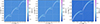 |
Fig. 4. Window function convolution matrix. The horizontal axis is presented on logarithmic scales to enhance the clarity of the data. The left panel displays the convolution matrix for the density power spectrum of the BGS data. The middle panel illustrates the convolution matrix for the momentum power spectrum of the DESI-PV data. The right panel exhibits the convolution matrix for the cross power spectrum between the BGS and DESI-PV data. |
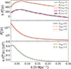 |
Fig. 5. Window function-convolved model power spectrum computed with different ℓmax values. The parameters of the power spectrum models are taken from Table 2. |
5. Tests on mocks
5.1. Fitting method
In this study, we concatenated the density, momentum, and cross power spectrum to effectively constrain the growth rate fσ8. By concatenating the models of these three spectrum, i.e. Eqs. (29), (30), and (31), we derived a comprehensive framework comprising 13 parameters in total. These encompass the growth rate, fσ8, the biasing parameters [b1σ8, b2σ8, bsσ8, b3nlσ8] for both the density and momentum fields, as well as the velocity dispersion parameters [σvS, σvT] for the density and momentum fields, respectively. However, in practical applications, it is not necessary to treat all 13 parameters as independent variables during model fitting with measurements, because these models are not equally sensitive to every parameter. Through the following testing using mocks, we discovered that a streamlined set of only five key parameters [ fσ8, b1σ8, b2σ8, σvT, σvS ] suffices to maintain robustness and precision in the fitting process (see Appendix E for more discussion). This led us to adopt a unified linear biasing parameter, b1σ8, for both the density and momentum fields, and a shared second-order biasing parameter, b2σ8, for both fields. Furthermore, we employed shared velocity dispersion parameters [σvT, σvS] across both the density and momentum fields.
In our study, the covariance matrix of the power spectrum is derived not from the actual Universe, but from a finite number of mocks. This limitation introduces an uncertainty into the inverse of the covariance matrix. This issue is referred to as the Hartlap effect (Hartlap et al. 2007). To address this challenge, we adopted the methodology proposed by Sellentin & Heavens (2016), which is different from the conventional approach of directly minimizing the χ2. Instead, we employed a likelihood function based on the following modified t distribution to derive more robust estimates of the parameters θ = [fσ8, b1σ8, b2σ8, σvT2, σvS2]:
![Mathematical equation: $$ \begin{aligned} \mathcal{L} (P|\theta ) \propto |\boldsymbol{\mathsf{C }}|^{-\frac{1}{2}} \left[ 1+\frac{ \chi ^2(P|\theta )}{N-1} \right]^{-\frac{N}{2}}, \end{aligned} $$](/articles/aa/full_html/2026/04/aa58368-25/aa58368-25-eq81.gif) (54)
(54)
where N = 675 is the number of mocks. Within this framework, the χ2 is formulated according to ![Mathematical equation: $ \chi^2(\boldsymbol{P}_{o}|\theta) = \left[ \mathbf{P}_{o}-\mathbf{P}^{c}_{m}(\theta)\right]\boldsymbol{\mathsf{C}}^{-1}\left[\mathbf{P}_{o}-\mathbf{P}^{c}_{m}(\theta)\right]^T $](/articles/aa/full_html/2026/04/aa58368-25/aa58368-25-eq82.gif) , where Po signifies the measured power spectrum,
, where Po signifies the measured power spectrum,  denotes the model power spectrum convolved with the survey window function, and C represents the covariance matrix.
In this research, cosmological parameters were extracted through a combination of the auto-density power spectrum monopole, P0δ, and quadrupole, P2δ, the auto-momentum power spectrum monopole, P0p, and the cross-power spectrum dipole, P1δp. Specifically, both Po = [P0δ, P2δ, P0p, P1δp] and Pmc = [P0δc, P2δc, P0pc, P1δpc] are represented as 4Nk vectors, while the covariance matrix, C, spans a dimensionality of 4Nk × 4Nk. Additional measured multipole components of the power spectrum of the survey data are found to be close to zero and exhibit high noise levels; therefore, they are excluded from the parameter estimation process in this work.
Parameter inference was conducted using the Metropolis-Hastings Markov chain Monte Carlo (MCMC) methodology, under uniformly flat priors defined over the interval fσ8 ∈ (0, 1.5], b1σ8 ∈ [0, 3], b2σ8 ∈ [ − 5, 5], σvT2 ∈ (0, 3502], and σvS2 ∈ (0, 3502]. Our growth rate constraints were obtained through the measurement of power spectrum in bins of k ∈ [0.025, 0.3], with bin widths of 0.009h Mpc−1.
5.2. Fitting fσ8 of the mocks
We began by fitting the power spectrum of the mock average. As is illustrated in Fig. 6, the filled circles represent the average of the power spectrum measured from 675 mocks, while the solid curves depict the best-fit theoretical models. The density power spectrum was measured from the BGS mocks, whereas the momentum power spectrum was obtained from the DESI-PV mocks. Each cross-power spectrum was computed using a BGS mock and its corresponding DESI-PV mock (which has the same observer as that BGS mock).
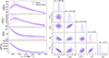 |
Fig. 6. Power spectrum and parameter fitting outcomes from the BGS and DESI-PV mocks. In the left panels, the filled circles represent the averaged measurements of the density monopole, density quadrupole, momentum monopole, and cross dipole power spectrum, respectively, across 675 mocks. The error bars reflect the uncertainty associated with a single realization. The fitted model power spectrum is overlaid as curves. On the right, the marginalized histograms and two-dimensional contours of the MCMC samples for the cosmological parameters are shown, with the MCMC fit results annotated at the top of each histogram (or see Table 2). The 2D contours delineate the 1, 1.5, 2, and 2.5σ confidence levels, while the shaded regions in the histograms indicate the 1σ confidence interval. The vertical dashed line marks the fiducial value fσ8 = 0.466. |
The MCMC resulting parameter estimates are summarized in Table 2 and illustrated in the right panel of Fig. 6. Notably, the estimated value of  closely aligns with the mock fiducial value of fσ8,fid = 0.466 at effective redshift zeff = 0.2. This agreement demonstrates that our fitting methodology effectively recovers the true growth rate embedded in the mocks, and that the power spectrum models perform robustly up to the non-linear scale of kmax = 0.3 h Mpc−1 under current conditions. In this analysis, we excluded the momentum power spectrum quadrupole, P2p, as it is heavily dominated by noise in survey data. To further assess the adaptability of our model, we also conducted fits incorporating P2p using the mock average, where P2p exhibits sufficient smoothness to yield a reliable fit. For a more detailed exploration, please refer to Appendix F.
MCMC-fit cosmological parameter estimates derived from mock average.
We proceeded to fit fσ8 of 15 randomly selected DESI-PV mocks and their corresponding BGS mock counterparts. As is illustrated in the top panel of Fig. 7, the filled squares represent the MCMC estimates of fσ8 derived from each of the 15 mock sets, all of which align closely with the fiducial fσ8 value (indicated by the dashed yellow line). The shaded blue band displays the fσ8 constraint extracted from Table 2 (i.e. mock average), providing an independent reference for comparison. The reduced χ2 values for all 15 measurements are found to be near unity, underscoring the robustness of the model and confirming that it provides an excellent statistical fit to the mock data. Figure 8 presents the growth rate constraints derived from fitting the power spectrum using different wave number cut-offs kmax, demonstrating that our models yield stable fits and reliable for kmax < 0.35 h Mpc−1.
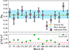 |
Fig. 7. fσ8 fit results (represented by filled squares in the top panel) from 15 randomly selected BGS mocks and their corresponding DESI-PV mock counterparts. In the top panel, the dashed yellow line indicates the fiducial value fσ8 = 0.466 of mocks. The blue band represents the fσ8 value from Table 2. The bottom panel illustrates the reduced χ2 values for each measurement, depicted by filled green circles. |
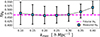 |
Fig. 8. fσ8 as a function of the cut-off wave number. The filled blue squares show the estimated fσ8 as a function of the cut-off wave number, kmax. The dashed pink line is the fiducial value 0.466. |
6. Results
6.1. The systematic error of the FP data
In Fig. 9, we compare the measured momentum power spectrum of the FP survey data with the average momentum power spectrum derived from 675 FP mocks. As the plot illustrates, the momentum power spectrum from the FP data begins to deviate. Specifically, it becomes elevated relative to the mocks starting at k = 0.05 h Mpc−1. This discrepancy becomes even more pronounced at k = 0.1 h Mpc−1, where the data exhibits significantly higher values than the mock predictions. This bias originates from a systematic bias in the measured η values of the FP data. In particular, within larger galaxy groups, the measured η tends to be more negative, leading to this anomalous behavior in the momentum power spectrum. This bias was initially identified by Howlett et al. (2022) through an analysis of the SDSSv data and has since been confirmed in DESI FP data, as reported by Ross et al. (2025). However, the underlying physical cause of this bias remains elusive and not yet fully understood. In future endeavours, a comprehensive galaxy group catalogue of DESI will be meticulously constructed, serving as a pivotal foundation for the calibration of this bias.
 |
Fig. 9. Comparison of the momentum power spectrum derived from the FP data (represented by filled magenta circles) with the averaged spectrum obtained from FP mocks (illustrated by filled blue circles accompanied by error bars). |
This systematic deviation also affects the estimation of fσ8, as the DESI-PV catalogue is predominantly composed of FP galaxies rather than TF galaxies. As is shown in the top panel of Fig. 10, the filled blue squares represent the estimated values of the growth rate, fσ8 (derived from the power spectrum of the BGS and DESI-PV data), as a function of the cut-off wave number, kmaxp, of the momentum power spectrum. We fixed kmax = 0.3 h Mpc−1 for the density and cross power spectrum. Notably, at  , the measured fσ8 abruptly rises from approximately 0.4 to around 0.6.
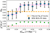 |
Fig. 10. In the top panel, the filled blue squares show the estimated growth rate, fσ8, as a function of the cut-off wave number, kmaxp, of the momentum power spectrum. We fixed kmax = 0.3 h Mpc−1 for the density and cross power spectrum. They were derived from the BGS and DESI-PV survey data. The dashed magenta line indicates the average of the filled blue squares. The dashed yellow line indicates the fiducial value fσ8 = 0.466 of mocks. The bottom panel illustrates the reduced χ2 values for each measurement, depicted by filled green circles. |
To mitigate this bias, we have to adopt a conservative approach by restricting the momentum power spectrum analysis to  when fitting fσ8 from survey data, while retaining kmax = 0.3 h Mpc−1 for the density and cross power spectrum. The information encoded in the momentum power spectrum is predominantly concentrated on the larger cosmological scales, specifically at wave numbers below k ≤ 0.1 h Mpc−1 (Howlett 2019; Bautista et al. 2025). Consequently, adopting a conservative cut-off at
  enables a robust analysis of the data without sacrificing significant signal content and does not impact our main conclusion.
It is important to emphasize that  reflects the reliability limit of the measured momentum power spectrum, rather than a breakdown of the theoretical model. Indeed, the model of momentum power spectrum remains robust and accurate up to kmax = 0.3 h Mpc−1 as demonstrated in Sect. 5.2. In future studies, with access to an unbiased velocity survey, we anticipate being able to extend the momentum power spectrum analysis to kmax = 0.3 h Mpc−1, thereby enhancing the precision and constraining power of our cosmological inferences.
6.2. Result of fσ8
As is depicted in Fig. 11, the power spectrum fitting results for the BGS and DESI-PV data are presented. In the left-hand panels, the top, middle, and bottom subplots display the measured density monopole and quadrupole, momentum monopole, and cross dipole power spectrum, respectively, with filled circles representing the measurements of the data. The curves illustrate the theoretical model spectrum that have been fitted to the measured data points. The goodness-of-fit is quantified by a reduced chi-squared value of χ2/d.o.f. = 116.563/(98 − 5) = 1.2534, indicating a satisfactory agreement between the model and the data. The derived cosmological parameter constraints are summarized in Table 3 and illustrated in the right panel of Fig. 11. Notably, the estimate for the growth rate is  at the effective redshift zeff = 0.07.
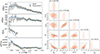 |
Fig. 11. Same as Fig. 6 but for the BGS data and DESI-PV data. In the right panel, the vertical dashed line marks the GR+Planck Collaboration VI (2020) prediction fσ8 = 0.446. The corresponding marginalized parameter values are summarized in Table 3. |
MCMC-fit cosmological parameter estimates derived from data.
To compute the theoretically predicted value of fσ8, we followed the formalism outlined in Howlett et al. (2015), wherein the growth rate as a function of redshift is expressed as
 (55)
(55)
with
 (56)
(56)
and Dgr(a) obtained from Eq. (45). Under the framework of GR, the growth index, γ, was fixed at 0.55 (Linder 2005). Consequently, with the Planck Collaboration VI (2020) cosmology, the GR predicts a growth rate of fσ8 = 0.446 at zeff = 0.07, which aligns remarkably well with our measured value of  at the 68% confidence level, underscoring the consistency between theory and observation.
The refined estimate of the growth rate, derived by synthesizing the fitting outcomes from the correlation function (Turner et al. 2025), maximum likelihood estimation (MLE, Lai et al. 2025), and the power spectrum of this paper, yields a consensus value of  , in concordance with theoretical predictions too. For a deeper exploration of data synthesis, see Bautista et al. (2025).
6.3. Result of γ
We present constraints on Linder’s growth index, γ (see Eq. (55)), assuming a ΛCDM background, obtained with cobaya (Torrado & Lewis 2021) interfaced to MGCAMB (Wang et al. 2023; Hojjati et al. 2011) using MG_flag = 2. In this setting, γ is mapped into the modified scale and redshift-dependent Poisson factor μ(a, k). In our analysis, we used DESI DR1 ShapeFit measurements in six redshift bins, distance-scale information from the post-reconstruction correlation function, and the baryon acoustic oscillation (BAO) Lyα likelihood used in DR1 (DESI Collaboration 2025d)6. We sampled the background parameters in addition to γ and report σ8 as a derived quantity. To mitigate projection effects, we applied a Big-Bang nucleosynthesis Gaussian prior, ωb ∼ 𝒩(0.02218, 0.00055), and a broad Gaussian prior on ns centred on the Planck fit value with standard deviation inflated by a factor of ten, π(ns)∼𝒩(0.9649, 0.042) (Planck Collaboration VI 2020). The addition of PV fσ8 measurements with DESI DR1 ShapeFit breaks the σ8–γ degeneracy and sharpens the constraints on all parameters.
Figure 12 shows the fitting results for (γ, Ωm, σ8) obtained from DESI DR1 ShapeFit (SF) + BAO, combined with our PV consensus,  (orange contours). We find
  ,
,  , and
, and  . Our result is consistent with GR. The PV fσ8 information reduced the errors of γ, Ωm, and σ8 by ≈32%, ≈33%, and ≈20% respectively, relative to SF+BAO alone (see blue contours or Table 4). Our measurement of γ falls notably below the values reported by Nguyen et al. (2023) and Calabrese et al. (2025), who obtain higher estimate values of γ ∼ 0.65.
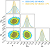 |
Fig. 12. Constraints on (γ, Ωm, σ8). DESI DR1 (SF+BAO; blue) and its combination with PV consensus fσ8 (orange). Shaded regions show 68% and 95% credible contours. The vertical dashed line marks the GR prediction γ = 0.55. |
Estimated values of γ, Ωm, and σ8.
7. Discussion
Figure 13 displays the evolution of the growth rate, fσ8, as a function of redshift, z. The blue curve was derived from Eq. (55), under the assumption of GR and a ΛCDM cosmological model based on Planck Collaboration VI (2020). The filled green circle represents the measurement derived from this paper. In comparison with the results presented in Turner et al. (2025) and Lai et al. (2025), our measurement exhibits slightly broader error margins, a consequence of adopting a lower wave number cut-off,  , in the analysis of the momentum power spectrum, relative to the higher thresholds employed in the other two studies. The filled red diamond denotes the consensus outcome of these three measurements. The other measurements are: H17: Howlett et al. (2017); J14: Johnson et al. (2014); A20: Adams & Blake (2020); Q19: Qin et al. (2019a); Q25: Qin et al. (2025); B12: Beutler et al. (2012); As23: Appleby et al. (2023); T23: Turner et al. (2023); D19: Dupuy et al. (2019); W18: Wang et al. (2018); C15: Carrick et al. (2015); S20: Said et al. (2020); Bp24: Boubel et al. (2024); Bs20: Boruah et al. (2020); DESI: DESI Collaboration (2025c); SDSS: Alam et al. (2021); B11 WiggleZ: Blake et al. (2011).
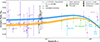 |
Fig. 13. Growth rate, fσ8, as a function of redshift, z. The blue curve represents the theoretical prediction derived under the assumption of GR (γ = 0.55) and a ΛCDM cosmology calibrated using Planck Collaboration VI (2020). The filled green circle denotes the measurement obtained in this study. The filled orange square corresponds to the result from Lai et al. (2025, using MLE), based on the same dataset, while the filled blue pentagon reflects the measurement from Turner et al. (2025, using correlation functions), also utilizing identical data. The filled red diamond corresponds to the consensus result of these three measurements. Additional observational constraints are illustrated by purple circles (using power spectrum), purple squares (using MLE), a purple cross (using reconstruction), and purple pentagons (using correlation functions), representing measurements from other surveys. The light blue pentagrams corresponds to the results from DESI DR1. The dashed orange curve indicates the model fits to all the data points, with the shaded orange region depicting the associated uncertainties. |
Although these measurements largely align with the predictions of GR, a subtle discrepancy becomes apparent when they are analysed in combination. To further investigate this, we integrated the aforementioned measured fσ8 values (i.e. all the data points in Fig. 13; we only used the filled red diamond for DESI-PV) with the Planck chain7 and performed a fitting analysis for γ. The resulting fit value of γ = 0.63 ± 0.02 was then transformed into a corresponding range of fσ8 values across different redshifts and is presented as the orange-coloured curve in Fig. 13. This result indicates a moderate tendency in the data towards a higher γ value, implying a potentially weaker gravitational model compared to the predictions of GR (blue curve in Fig. 13). However, it is important to note that the fit value and associated uncertainty for this γ should be interpreted with caution, as there exists considerable overlap – and thus covariance – among many of the measurements in Fig. 13, which has not been fully incorporated into the analysis. Nonetheless, as is shown in Fig. 13, a minor tension remains between current observational data and the theoretical predictions of GR, a discrepancy that may be further clarified or resolved through future research and surveys.
8. Conclusions
In this paper, we build upon the foundational research presented in Paper I, Paper II, and Paper III by conducting a comprehensive joint analysis of the monopole and quadrupole moments of the auto-density power spectrum, the monopole of the auto-momentum power spectrum, and the dipole component of the cross-power spectrum to measure the growth rate, fσ8. The density field was derived from the BGS, whereas the momentum field was extracted from the DESI-PV. Our investigation yields the following key findings:
-
We have systematically presented the power spectrum estimators and the window function convolution matrix.
-
We have refined the theoretical model of the cross-power spectrum and extended its applicability to scenarios in which the density and momentum fields originate from different survey catalogues.
-
Utilizing mocks, we demonstrate that the power spectrum models exhibit robust performance up to the non-linear scale of kmax = 0.3 h Mpc−1 when fitting fσ8 using the set [P0δ, P2δ, P0p, P1δp] and treating [fσ8, b1σ8, b2σ8, σvT2, σvS2] as free parameters.
-
Furthermore, our analysis of mocks reveals that the models remain reliable up to the non-linear scale of kmax = 0.25 h Mpc−1 when fitting fσ8 using [P0δ, P2δ, P0p, P2p, P1δp] and allowing
![Mathematical equation: $ {[f\sigma_{8}, b^{\delta}_{1}\sigma_{8}, b_{2}\sigma_{8}, b^p_{1}\sigma_{8}, \sigma^2_{\delta,vT}, \sigma^2_{vS}, \sigma^2_{p,vT}]} $](/articles/aa/full_html/2026/04/aa58368-25/aa58368-25-eq115.gif) to vary freely.
to vary freely. -
Our results indicate that the systematic bias of FP data enhances the measured momentum power spectrum at k > 0.1 h Mpc−1. Consequently, we restrict our fitting range of the momentum power spectrum to k ≤ 0.1 h Mpc−1 to mitigate this effect.
-
We obtain an estimate of the growth rate as
 at zeff = 0.07. The refined estimate of the growth rate, derived by synthesizing the fitting outcomes from Turner et al. (2025), Lai et al. (2025), and this paper, yields a consensus value of fσ8 = 0.450 ± 0.055. These are in agreement with the prediction of the ΛCDM and GR models.
 -
We obtain an estimate of γ as
 (corresponding to the consensus fσ8), which is in agreement with the prediction of GR. Correspondingly, we find
  and
and  .
.
There are several promising avenues for future research building upon this work. (1) Our methodology can be applied to Data Release 2 of the DESI peculiar velocity survey, which is significantly more homogeneous and extensive than Data Release 1, thereby enabling a more precise constraint on fσ8. (2) While the current analysis assumes the local plane-parallel approximation, future efforts will focus on incorporating wide-angle effects into both our models and estimators. (3) As is highlighted in Appendix G of this paper, the momentum power spectrum and cross power spectrum lack Galilean invariance, making them susceptible to potential systematic biases in the data. To address this limitation, we aim to transition toward measuring and modelling the pair-wise momentum power spectrum, as has been proposed by Chen et al. (2025). (4) We have not yet accounted for the gravitational redshift of galaxies. In forthcoming studies, we intend to extend our framework to measure and model this relativistic effect, following the approach outlined by Beutler & Di Dio (2020).
Data availability
The data used to generate the figures in this paper are available at https://zenodo.org/uploads/17672675
Acknowledgments
FQ and JB is supported by the funding from Excellence Initiative of Aix-Marseille University – A*MIDEX, a French “Investissements d’Avenir” program (AMX-20-CE-02 – DARKUNI). This material is based upon work supported by the U.S. Department of Energy (DOE), Office of Science, Office of High-Energy Physics, under Contract No. DE–AC02–05CH11231, and by the National Energy Research Scientific Computing Center, a DOE Office of Science User Facility under the same contract. Additional support for DESI was provided by the U.S. National Science Foundation (NSF), Division of Astronomical Sciences under Contract No. AST-0950945 to the NSF’s National Optical-Infrared Astronomy Research Laboratory; the Science and Technology Facilities Council of the United Kingdom; the Gordon and Betty Moore Foundation; the Heising-Simons Foundation; the French Alternative Energies and Atomic Energy Commission (CEA); the National Council of Humanities, Science and Technology of Mexico (CONAHCYT); the Ministry of Science, Innovation and Universities of Spain (MICIU/AEI/10.13039/501100011033), and by the DESI Member Institutions: https://www.desi.lbl.gov/collaborating-institutions. Any opinions, findings, and conclusions or recommendations expressed in this material are those of the author(s) and do not necessarily reflect the views of the U.S. National Science Foundation, the U.S. Department of Energy, or any of the listed funding agencies. The authors are honored to be permitted to conduct scientific research on I’oligam Du’ag (Kitt Peak), a mountain with particular significance to the Tohono O’odham Nation.
References
- Abate, A., Bridle, S., Teodoro, L. F. A., Warren, M. S., & Hendry, M. 2008, MNRAS, 389, 1739 [NASA ADS] [CrossRef] [Google Scholar]
- Adams, C., & Blake, C. 2017, MNRAS, 471, 839 [NASA ADS] [CrossRef] [Google Scholar]
- Adams, C., & Blake, C. 2020, MNRAS, 494, 3275 [NASA ADS] [CrossRef] [Google Scholar]
- Alam, S., Aubert, M., Avila, S., et al. 2021, Phys. Rev. D, 103, 083533 [NASA ADS] [CrossRef] [Google Scholar]
- Appleby, S., Tonegawa, M., Park, C., et al. 2023, ApJ, 958, 180 [Google Scholar]
- Bautista, J., Amsellem, A. J., Aronica, V., et al. 2025, arXiv e-prints [arXiv:2512.03228] [Google Scholar]
- Beutler, F., & Di Dio, E. 2020, JCAP, 2020, 048 [CrossRef] [Google Scholar]
- Beutler, F., Blake, C., Colless, M., et al. 2012, MNRAS, 423, 3430 [NASA ADS] [CrossRef] [Google Scholar]
- Bianchi, D., Gil-Marín, H., Ruggeri, R., & Percival, W. J. 2015, MNRAS, 453, L11 [NASA ADS] [CrossRef] [Google Scholar]
- Blake, C., & Turner, R. J. 2024, Open J. Astrophys., 7, 87 [Google Scholar]
- Blake, C., Brough, S., Colless, M., et al. 2010, MNRAS, 406, 803 [NASA ADS] [Google Scholar]
- Blake, C., Brough, S., Colless, M., et al. 2011, MNRAS, 415, 2876 [NASA ADS] [CrossRef] [Google Scholar]
- Blake, C., Carter, P., & Koda, J. 2018, MNRAS, 479, 5168 [Google Scholar]
- Boruah, S. S., Hudson, M. J., & Lavaux, G. 2020, MNRAS, 498, 2703 [Google Scholar]
- Boruah, S. S., Lavaux, G., & Hudson, M. J. 2022, MNRAS, 517, 4529 [NASA ADS] [CrossRef] [Google Scholar]
- Boubel, P., Colless, M., Said, K., & Staveley-Smith, L. 2024, MNRAS, 531, 84 [Google Scholar]
- Calabrese, E., Hill, J. C., Jense, H. T., et al. 2025, JCAP, 2025, 063 [Google Scholar]
- Campbell, L. A., Lucey, J. R., Colless, M., et al. 2014, MNRAS, 443, 1231 [NASA ADS] [CrossRef] [Google Scholar]
- Carr, A., Howlett, C., Amsellem, A. J., et al. 2025, arXiv e-prints [arXiv:2512.03232] [Google Scholar]
- Carreres, B., Bautista, J. E., Feinstein, F., et al. 2023, A&A, 674, A197 [NASA ADS] [CrossRef] [EDP Sciences] [Google Scholar]
- Carrick, J., Turnbull, S. J., Lavaux, G., & Hudson, M. J. 2015, MNRAS, 450, 317 [Google Scholar]
- Castorina, E., & White, M. 2020, MNRAS, 499, 893 [Google Scholar]
- Chen, S. F., Howlett, C., Lai, Y., & Qin, F. 2025, arXiv e-prints [arXiv:2508.00066] [Google Scholar]
- Courtois, H. M., Pomarède, D., Tully, R. B., Hoffman, Y., & Courtois, D. 2013, AJ, 146, 69 [NASA ADS] [CrossRef] [Google Scholar]
- Davis, T. M., & Scrimgeour, M. I. 2014, MNRAS, 442, 1117 [NASA ADS] [CrossRef] [Google Scholar]
- DESI Collaboration (Aghamousa, A., et al.) 2016a, arXiv e-prints [arXiv:1611.00036] [Google Scholar]
- DESI Collaboration (Aghamousa, A., et al.) 2016b, arXiv e-prints [arXiv:1611.00037] [Google Scholar]
- DESI Collaboration (Abareshi, B., et al.) 2022, AJ, 164, 207 [NASA ADS] [CrossRef] [Google Scholar]
- DESI Collaboration (Adame, A. G., et al.) 2024a, AJ, 168, 58 [NASA ADS] [CrossRef] [Google Scholar]
- DESI Collaboration (Adame, A. G., et al.) 2024b, AJ, 167, 62 [NASA ADS] [CrossRef] [Google Scholar]
- DESI Collaboration (Abdul-Karim, M., et al.) 2025a, arXiv e-prints [arXiv:2503.14745] [Google Scholar]
- DESI Collaboration (Abdul Karim, M., et al.) 2025b, Phys. Rev. D, 112, 083515 [Google Scholar]
- DESI Collaboration (Adame, A. G., et al.) 2025c, JCAP, 2025, 028 [Google Scholar]
- DESI Collaboration (Adame, A. G., et al.) 2025d, JCAP, 2025, 124 [CrossRef] [Google Scholar]
- DESI Collaboration (Adame, A. G., et al.) 2025e, JCAP, 2025, 017 [Google Scholar]
- DESI Collaboration (Adame, A. G., et al.) 2025f, JCAP, 2025, 008 [Google Scholar]
- Djorgovski, S., & Davis, M. 1987, ApJ, 313, 59 [Google Scholar]
- Douglass, K., BenZvi, S., Kim, A. G., et al. 2025, arXiv e-prints [arXiv:2512.03227] [Google Scholar]
- Dressler, A., Lynden-Bell, D., Burstein, D., et al. 1987, ApJ, 313, 42 [Google Scholar]
- Dupuy, A., & Courtois, H. M. 2023, A&A, 678, A176 [NASA ADS] [CrossRef] [EDP Sciences] [Google Scholar]
- Dupuy, A., Courtois, H. M., & Kubik, B. 2019, MNRAS, 486, 440 [NASA ADS] [CrossRef] [Google Scholar]
- Feldman, H. A., Kaiser, N., & Peacock, J. A. 1994, ApJ, 426, 23 [Google Scholar]
- Feldman, H. A., Watkins, R., & Hudson, M. J. 2010, MNRAS, 407, 2328 [Google Scholar]
- Gorski, K. M., Davis, M., Strauss, M. A., White, S. D. M., & Yahil, A. 1989, ApJ, 344, 1 [NASA ADS] [CrossRef] [Google Scholar]
- Guy, J., Bailey, S., Kremin, A., et al. 2023, AJ, 165, 144 [NASA ADS] [CrossRef] [Google Scholar]
- Hahn, C., Wilson, M. J., Ruiz-Macias, O., et al. 2023, AJ, 165, 253 [CrossRef] [Google Scholar]
- Hartlap, J., Simon, P., & Schneider, P. 2007, A&A, 464, 399 [NASA ADS] [CrossRef] [EDP Sciences] [Google Scholar]
- Heath, D. J. 1977, MNRAS, 179, 351 [NASA ADS] [CrossRef] [Google Scholar]
- Hojjati, A., Pogosian, L., & Zhao, G.-B. 2011, JCAP, 08, 005 [CrossRef] [Google Scholar]
- Hong, T., Staveley-Smith, L., Masters, K. L., et al. 2019, MNRAS, 487, 2061 [Google Scholar]
- Hong, S. E., Jeong, D., Hwang, H. S., & Kim, J. 2021, ApJ, 913, 76 [Google Scholar]
- Howlett, C. 2019, MNRAS, 487, 5209 [Google Scholar]
- Howlett, C., Ross, A. J., Samushia, L., Percival, W. J., & Manera, M. 2015, MNRAS, 449, 848 [NASA ADS] [CrossRef] [Google Scholar]
- Howlett, C., Staveley-Smith, L., Elahi, P. J., et al. 2017, MNRAS, 471, 3135 [NASA ADS] [CrossRef] [Google Scholar]
- Howlett, C., Said, K., Lucey, J. R., et al. 2022, MNRAS, 515, 953 [NASA ADS] [CrossRef] [Google Scholar]
- Ishak, M. 2019, Liv. Rev. Rel., 22, 1 [NASA ADS] [CrossRef] [Google Scholar]
- Ishak, M., Pan, J., Calderon, R., et al. 2025, JCAP, 2025, 053 [Google Scholar]
- Johnson, A., Blake, C., Koda, J., et al. 2014, MNRAS, 444, 3926 [NASA ADS] [CrossRef] [Google Scholar]
- Kaiser, N. 1987, MNRAS, 227, 1 [Google Scholar]
- Kaiser, N. 1988, MNRAS, 231, 149 [NASA ADS] [Google Scholar]
- Kaiser, N., & Peacock, J. A. 1991, ApJ, 379, 482 [Google Scholar]
- Karamanis, M., & Beutler, F. 2021, https://doi.org/10.5281/zenodo.4923137 [Google Scholar]
- Kitaura, F.-S., Angulo, R. E., Hoffman, Y., & Gottlöber, S. 2012, MNRAS, 425, 2422 [Google Scholar]
- Koda, J., Blake, C., Davis, T., et al. 2014, MNRAS, 445, 4267 [NASA ADS] [CrossRef] [Google Scholar]
- Lai, Y., Howlett, C., & Davis, T. M. 2023, MNRAS, 518, 1840 [Google Scholar]
- Lai, Y., Howlett, C., Aguilar, J., et al. 2025, arXiv e-prints [arXiv:2512.03229] [Google Scholar]
- Levi, M., Bebek, C., Beers, T., et al. 2013, arXiv e-prints [arXiv:1308.0847] [Google Scholar]
- Lewis, A., Challinor, A., & Lasenby, A. 2000, ApJ, 538, 473 [Google Scholar]
- Linder, E. V. 2005, Phys. Rev. D, 72, 043529 [Google Scholar]
- Lyall, S., Blake, C., Turner, R., Ruggeri, R., & Winther, H. 2023, MNRAS, 518, 5929 [Google Scholar]
- Maksimova, N. A., Garrison, L. H., Eisenstein, D. J., et al. 2021, MNRAS, 508, 4017 [NASA ADS] [CrossRef] [Google Scholar]
- McDonald, P., & Roy, A. 2009, JCAP, 2009, 020 [CrossRef] [Google Scholar]
- Miller, T. N., Doel, P., Gutierrez, G., et al. 2024, AJ, 168, 95 [NASA ADS] [CrossRef] [Google Scholar]
- Nguyen, N.-M., Huterer, D., & Wen, Y. 2023, Phys. Rev. Lett., 131, 111001 [CrossRef] [Google Scholar]
- Nguyen, A., Blake, C., Turner, R. J., et al. 2025, arXiv e-prints [arXiv:2510.07673] [Google Scholar]
- Nusser, A., Dekel, A., Bertschinger, E., & Blumenthal, G. R. 1991, ApJ, 379, 6 [NASA ADS] [CrossRef] [Google Scholar]
- Okumura, T., Seljak, U., Vlah, Z., & Desjacques, V. 2014, JCAP, 2014, 003 [Google Scholar]
- Park, C. 2000, MNRAS, 319, 573 [Google Scholar]
- Park, C.-G., & Park, C. 2006, ApJ, 637, 1 [Google Scholar]
- Planck Collaboration VI. 2020, A&A, 641, A6 [NASA ADS] [CrossRef] [EDP Sciences] [Google Scholar]
- Poppett, C., Tyas, L., Aguilar, J., et al. 2024, AJ, 168, 245 [Google Scholar]
- Qin, F. 2021, Res. Astron. Astrophys., 21, 242 [Google Scholar]
- Qin, F., Howlett, C., Staveley-Smith, L., & Hong, T. 2018, MNRAS, 477, 5150 [Google Scholar]
- Qin, F., Howlett, C., & Staveley-Smith, L. 2019a, MNRAS, 487, 5235 [CrossRef] [Google Scholar]
- Qin, F., Howlett, C., Staveley-Smith, L., & Hong, T. 2019b, MNRAS, 482, 1920 [Google Scholar]
- Qin, F., Parkinson, D., Howlett, C., & Said, K. 2021, ApJ, 922, 59 [Google Scholar]
- Qin, F., Howlett, C., Stevens, A. R. H., & Parkinson, D. 2022, ApJ, 937, 113 [Google Scholar]
- Qin, F., Parkinson, D., Hong, S. E., & Sabiu, C. G. 2023a, JCAP, 2023, 062 [CrossRef] [Google Scholar]
- Qin, F., Parkinson, D., Stevens, A. R. H., & Howlett, C. 2023b, ApJ, 957, 40 [Google Scholar]
- Qin, F., Howlett, C., & Parkinson, D. 2025, ApJ, 978, 7 [Google Scholar]
- Ravoux, C., Carreres, B., Rosselli, D., et al. 2025, A&A, 698, A273 [NASA ADS] [CrossRef] [EDP Sciences] [Google Scholar]
- Rocher, A., Ruhlmann-Kleider, V., Burtin, E., et al. 2023, JCAP, 2023, 016 [CrossRef] [Google Scholar]
- Ross, C. E., Howlett, C., Lucey, J. R., et al. 2025, arXiv e-prints [arXiv:2512.03226] [Google Scholar]
- Said, K., Colless, M., Magoulas, C., Lucey, J. R., & Hudson, M. J. 2020, MNRAS, 497, 1275 [NASA ADS] [CrossRef] [Google Scholar]
- Saito, S., Baldauf, T., Vlah, Z., et al. 2014, Phys. Rev. D, 90, 123522 [NASA ADS] [CrossRef] [Google Scholar]
- Schlafly, E. F., Kirkby, D., Schlegel, D. J., et al. 2023, AJ, 166, 259 [NASA ADS] [CrossRef] [Google Scholar]
- Scrimgeour, M. I., Davis, T. M., Blake, C., et al. 2016, MNRAS, 455, 386 [Google Scholar]
- Sellentin, E., & Heavens, A. F. 2016, MNRAS, 456, L132 [Google Scholar]
- Shi, Y., Zhang, P., Mao, S., & Gu, Q. 2024, MNRAS, 528, 4922 [NASA ADS] [CrossRef] [Google Scholar]
- Silber, J. H., Fagrelius, P., Fanning, K., et al. 2023, AJ, 165, 9 [NASA ADS] [CrossRef] [Google Scholar]
- Smith, R. E. 2009, MNRAS, 400, 851 [NASA ADS] [CrossRef] [Google Scholar]
- Strauss, M. A., & Willick, J. A. 1995, Phys. Rep., 261, 271 [NASA ADS] [CrossRef] [Google Scholar]
- Torrado, J., & Lewis, A. 2021, JCAP, 05, 057 [Google Scholar]
- Tully, R. B., & Fisher, J. R. 1977, A&A, 54, 661 [NASA ADS] [Google Scholar]
- Turner, R. J., & Blake, C. 2023, MNRAS, 526, 337 [Google Scholar]
- Turner, R. J., Blake, C., & Ruggeri, R. 2021, MNRAS, 502, 2087 [Google Scholar]
- Turner, R. J., Blake, C., & Ruggeri, R. 2023, MNRAS, 518, 2436 [Google Scholar]
- Turner, R. J., Blake, C., Qin, F., et al. 2025, arXiv e-prints [arXiv:2512.03230] [Google Scholar]
- Vlah, Z., Seljak, U., McDonald, P., Okumura, T., & Baldauf, T. 2012, JCAP, 2012, 009 [CrossRef] [Google Scholar]
- Vlah, Z., Seljak, U., Okumura, T., & Desjacques, V. 2013, JCAP, 2013, 053 [Google Scholar]
- Wang, H., Mo, H. J., Yang, X., & van den Bosch, F. C. 2012, MNRAS, 420, 1809 [NASA ADS] [CrossRef] [Google Scholar]
- Wang, Y., Rooney, C., Feldman, H. A., & Watkins, R. 2018, MNRAS, 480, 5332 [Google Scholar]
- Wang, Z., Mirpoorian, S. H., Pogosian, L., Silvestri, A., & Zhao, G.-B. 2023, JCAP, 08, 038 [Google Scholar]
- Watkins, R., & Feldman, H. A. 2015, MNRAS, 450, 1868 [NASA ADS] [CrossRef] [Google Scholar]
- Whitford, A. M., Howlett, C., & Davis, T. M. 2023, MNRAS, 526, 3051 [NASA ADS] [CrossRef] [Google Scholar]
- Wu, Z., Xiao, L., Xiao, X., et al. 2023, MNRAS, 522, 4748 [NASA ADS] [Google Scholar]
- Yamamoto, K., Nakamichi, M., Kamino, A., Bassett, B. A., & Nishioka, H. 2006, PASJ, 58, 93 [Google Scholar]
- Zhang, Y., Qin, F., & Wang, B. 2017, Phys. Rev. D, 96, 103523 [Google Scholar]
abacus_cosm000: https://abacussummit.readthedocs.io/en/latest/cosmologies.html
The HANKL PYTHON package: https://hankl.readthedocs.io/en/latest/install.html
CAMB: https://camb.info/
For details regarding the ShapeFit compression, we direct readers to Sect. 4 of DESI Collaboration (2025f).
We use the chain base_plikHM_TTTEEE_lowl_lowE_lensing_1.txt in CosmoParams_base-plikHM_R3.01 on https://irsa.ipac.caltech.edu/data/Planck/release_3/ancillary-data/ as a prior on Ωm.
Appendix A: Peculiar velocity estimator
By employing the low-redshift approximation of the log-distance ratio, and under the assumption that the true peculiar velocities of galaxies are significantly smaller than their observed redshifts, the line-of-sight peculiar velocities can then be inferred from η through (Johnson et al. 2014; Watkins & Feldman 2015; Adams & Blake 2017; Howlett et al. 2017; Qin et al. 2018; Carreres et al. 2023)
 (A.1)
(A.1)
where zmod is given by (Davis & Scrimgeour 2014; Watkins & Feldman 2015)
![Mathematical equation: $$ \begin{aligned} z_{\mathrm{mod} }=z\left[1+\frac{1}{2}(1-q_0)z-\frac{1}{6}(1-q_0-3q_0^2+1)z^2\right]\,, \end{aligned} $$](/articles/aa/full_html/2026/04/aa58368-25/aa58368-25-eq121.gif) (A.2)
(A.2)
and where z is the observed redshift of a galaxy. The acceleration parameter is q0 = 0.5(Ωm − 2ΩΛ).
Following the methodology outlined in Watkins & Feldman (2015) and Paper II, we adopt the following for Eq. 26
 (A.3)
(A.3)
where ση denotes the measurement error in the log-distance ratio η. 3002 km2 s−2 represents the intrinsic scatter in peculiar velocities caused by non-linear galactic motions. As discussed in Appendix A of Paper II, variations in the assumed value of this intrinsic scatter have minimal impact on our results. The ⟨v2(r)⟩ term for the DESI-PV random catalogue is computed by Bautista et al. (2025).
Appendix B: Verifying  for cross-power spectrum
In Sect. 3.2, we indicated that the estimator of the cross-power spectrum given in Eq. 17 should satisfy the condition  . This property will be verified in the present section. To begin with, let i denote the imaginary unit, such that i2 = −1. Upon disregarding the shot-noise term and referring to Eq. 17, we obtain
 (B.1)
(B.1)
which subsequently implies
 (B.2)
(B.2)
On the other hand, we have
 (B.3)
(B.3)
which subsequently implies
 (B.4)
(B.4)
Comparing the above equation to Eq. B.2, one can logically infer that  .
.
Appendix C: The linear models of power spectrum and the models for the correlation functions
Kaiser (1987) developed a linear model for the density power spectrum, commonly referred to as the Kaiser Formula, given by
 (C.1)
(C.1)
which has been extensively utilized over the past decades. Building upon this foundation, Koda et al. (2014) extended the analysis to the power spectrum of peculiar velocities as well as cross-power, they modelling the velocity power spectrum and density-velocity cross power spectrum using
 (C.2)
(C.2)
 (C.3)
(C.3)
Furthermore, they incorporated damping terms into the above linear models in order to more accurately account for non-linear motions of galaxies, given by
 (C.4)
(C.4)
 (C.5)
(C.5)
 (C.6)
(C.6)
where the damping terms are defined by
 (C.7)
(C.7)
to account for non-linear motions of galaxies. The σg and σv are the non-linear velocity dispersion parameters for the density and velocity fields, respectively.
We initialize all loop terms–Imn, Kmn, Kmns, σ3 and σ4–to zero, and similarly set the higher-order biasing and velocity dispersion parameters to zeros. In essence, we retain only fσ8 and b1σ8. Consequently, Eq. 29, 30 and 31 reduce to the classic Kaiser formulae expressed in Eq. C.1,C.2 and C.3, respectively, as illustrated in Fig.C.2. For simplicity, we manually set fσ8 = 0.437, b1σ8 = 0.564 and effective redshift z = 0 to generate this plot. In the middel panel of Fig. C.2, it becomes evident that the momentum power spectrum quadrupole P2p (represented by yellow dots and the yellow curve) surpasses the monopole P0p (depicted by blue dots and its curve). This arises due to the absence of window function convolution effects in our current consideration. Illustrated in Fig.C.1 is the linear matter power spectrum utilized in our analysis.
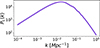 |
Fig. C.1. Linear matter power spectrum PL(k). |
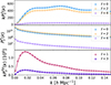 |
Fig. C.2. Comparing the Kaiser formulas (filled circles), Eqs. C.1, C.2, and C.3 to the linearized perturbation models (curves) Eqs. 29, 30, and 31. |
The mathematical framework for converting power spectrum to correlation functions primarily draws upon Turner et al. (2025). In Fig.C.3, we present the model correlation functions converted from the power spectrum models presented in Sect. 4 with parameters from Table 2.
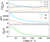 |
Fig. C.3. Two-point correlation function models are derived from the power spectrum models introduced in Sect. 4, using the parameter values listed in Table 2. The top panel illustrates the galaxy auto-two-point correlation function |


Appendix D: The multipoles of the field function
The Eq. 19 can be further expressed in a more refined form as
 (D.1)
(D.1)
Thus, by directly expanding the term  for ℓ = 0, 2 and 4, the even-multipole components of the Fourier-transformed field function are explicitly presented in
 (D.2)
(D.2)
 (D.3)
(D.3)
and
 (D.4)
(D.4)
respectively, and where
 (D.5)
(D.5)
where i, j, n = x, y, z.
Furthermore, guided by the theoretical framework proposed in Paper III, based on Eq. D.1, the odd-multipole components of the Fourier-transformed field function are formulated as described in
 (D.6)
(D.6)
 (D.7)
(D.7)
and where
 (D.8)
(D.8)
where i, j, n = x, y, z.
Appendix E: More tests using mocks
In Sect. 5.2 we demonstrate the adaptability of the power spectrum models by performing fits on [P0δ, P2δ, P0p, P1δp] using five free parameters [ fσ8, b1σ8, b2σ8, σvT, σvS ], which suffices to maintain robustness and precision in the fitting process. Alternatively, we can separate the biasing parameters between the density and momentum fields–i.e., adopt seven free parameters ![Mathematical equation: $ {[\ f\sigma_8,\ b^{\delta}_{1}\sigma_8,\ b^{\delta}_{2}\sigma_8,\ b^p_{1}\sigma_8,\ b^p_{2}\sigma_8,\ \sigma_{vT},\ \sigma_{vS}\ ]} $](/articles/aa/full_html/2026/04/aa58368-25/aa58368-25-eq148.gif) –without significantly altering the resulting fσ8; see Fig.E.1. Consequently, to maintain model simplicity and reduce parameters, we adopt shared biasing parameters for both fields.
–without significantly altering the resulting fσ8; see Fig.E.1. Consequently, to maintain model simplicity and reduce parameters, we adopt shared biasing parameters for both fields.
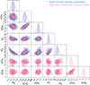 |
Fig. E.1. Fitting results obtained with |
![Mathematical equation: $ {[\ f\sigma_8,\ b^{\delta}_{1}\sigma_8,\ b^{\delta}_{2}\sigma_8,\ b^p_{1}\sigma_8,\ b^p_{2}\sigma_8,\sigma_{vT},\sigma_{vS}\ ] } $](/articles/aa/full_html/2026/04/aa58368-25/aa58368-25-eq149.gif)
Appendix F: Fitting fσ8 of mocks from 
In Sect. 5.2 we demonstrate the adaptability of the power spectrum models by performing fits on [P0δ, P2δ, P0p, P1δp]. Given that the momentum power spectrum quadrupole P2p derived from the FP mock average displays a sufficiently smooth behavior to support a robust fitting procedure, we extend our analysis to include P2p in the parameter estimation, thereby enabling a more comprehensive determination of fσ8 based on [P0δ, P2δ, P0p, P2p, P1δp].
As we incorporate additional data into the fitting process, it becomes essential to enhance the flexibility of the power spectrum models accordingly. To achieve this, we introduce two additional free parameters. Specifically, we distinguish the linear biasing parameters between the density and momentum fields, and similarly differentiate the velocity dispersion parameters across these two fields. Consequently, the set of free parameters is defined as ![Mathematical equation: $ \theta = [f\sigma_{8}, b^{\delta}_{1}\sigma_{8}, b_{2}\sigma_{8}, b^p_{1}\sigma_{8}, \sigma^2_{\delta,vT}, \sigma^2_{vS}, \sigma^2_{p,vT}] $](/articles/aa/full_html/2026/04/aa58368-25/aa58368-25-eq151.gif) , resulting in a total of seven independent parameters. All other parameters remain shared between the density and momentum fields. Furthermore, to ensure model stability and prevent breakdown at nonlinear scales, we adopt a reduced kmax value of 0.25 h Mpc−1, in contrast to that used in Sect. 5.2.
, resulting in a total of seven independent parameters. All other parameters remain shared between the density and momentum fields. Furthermore, to ensure model stability and prevent breakdown at nonlinear scales, we adopt a reduced kmax value of 0.25 h Mpc−1, in contrast to that used in Sect. 5.2.
As illustrated in Fig. F.1, the filled circles represent the average of the power spectrum measured from 675 mocks, while the solid curves depict the theoretical models fit to the measurements. The MCMC resulting parameter estimates are show in Fig.F.2 and summarized in Table F.1. The fit value of  , which well aligns with the fiducial simulation value of fσ8, fid = 0.466 at effective redshift zeff = 0.2. This agreement demonstrates that our fitting methodology effectively recovers the true growth rate embedded in the mocks, and that the power spectrum models perform robustly up to the non-linear scale of kmax = 0.25 h Mpc−1 under current conditions.
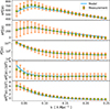 |
Fig. F.1. Same as Fig. 6 but for including the momentum power spectrum quadrupole P2p in the fitting. |
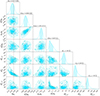 |
Fig. F.2. Same as Fig. 6 but for including the momentum power spectrum quadrupole P2p in the fitting. The corresponding marginalized parameter values are summarized in Table F.1. |
MCMC-fit cosmological parameter estimates.
Appendix G: The Galilean transformation of power spectrum
As elaborated in Paper III, the momentum power spectrum Pp(k) and cross-power spectrum Pδp(k) are not invariant under the Galilean transformation; that is, their values depend on the bulk motion of the sample relative to the observational frame. Specifically, for the momentum power spectrum, if a constant bulk velocity shift ϵ is introduced to the line-of-sight peculiar velocities, i.e., by substituting v(r)→v(r)+ϵ, the momentum correlation yields
 (G.1)
(G.1)
In this expression, the average of the density contrast field, i.e. ⟨δ(r)⟩ and ⟨δ(r′)⟩ are zeros. The average of the momentum field, i.e. ⟨p(r)⟩ and ⟨p(r′)⟩ are zeros too. Consequently, the above equation simplifies to
 (G.2)
(G.2)
Applying the Fourier transform to the aforementioned equation yields
![Mathematical equation: $$ \begin{aligned}&\frac{1}{(2\pi )^6}\int \langle p_G(\mathbf{k}) p^*_G(\mathbf{k}^{\prime }) \rangle e^{-i \mathbf{k} \cdot \mathbf{r} } e^{i \mathbf{k}^{\prime } \cdot \mathbf{r}^{\prime } } d^3kd^3k^{\prime } \nonumber \\ =&\frac{1}{(2\pi )^6}\int \Big [ \langle p(\mathbf{k}) p^*(\mathbf{k}^{\prime }) \rangle +\langle \delta ^*(\mathbf{k}^{\prime })p(\mathbf{k}) \rangle \epsilon +\langle \delta (\mathbf{k})p^*(\mathbf{k}^{\prime }) \rangle \epsilon \nonumber \\&+\langle \delta (\mathbf{k})\delta ^*(\mathbf{k}^{\prime })\rangle \epsilon ^2\Big ]e^{-i \mathbf{k} \cdot \mathbf{r} } e^{i \mathbf{k}^{\prime } \cdot \mathbf{r}^{\prime } } d^3kd^3k^{\prime } + \epsilon ^2 \delta ^D(\mathbf{k}) \delta ^D(\mathbf{k}^{\prime }) \end{aligned} $$](/articles/aa/full_html/2026/04/aa58368-25/aa58368-25-eq162.gif) (G.3)
(G.3)
in the final term, the δD(k) and δD(k′) cannot equal unity simultaneously, as we are exclusively considering the case k ≠ k′ in the context of two-point statistic. Consequently, δD(k)δD(k′) = 0, and the above equation indicates
 (G.4)
(G.4)
Substituting the definitions of the power spectrum provided in Eq. 3, 4 and 5 into the above equation leads to
 (G.5)
(G.5)
Given that Pδp = −Pδp* (see Appendix B), the above equation further reduces to
 (G.6)
(G.6)
which represents the Galilean-transformed form of the momentum power spectrum. Analogously, the corresponding Galilean-transformed cross-power spectrum is expressed as
 (G.7)
(G.7)
The bulk velocity ϵ comprises two possible components: one stems from coherent bulk motion of galaxies driven by local gravitational fluctuations, and the other originates from potential systematic errors induced by observational or measurement inaccuracies.
We investigate whether the fitting outcomes exhibit sensitivity to the parameter ϵ. By substituting the power spectrum models described in Sect. 4 into Eqs. G.6 and G.7, we obtain the Galilean-transformed versions of these models. These transformed models are then fitted to the measured power spectrum of BGS and DESI-PV data. In this analysis, ϵ is treated as a free parameter with a flat prior over the broad range of ϵ ∈ [ − 1000, 1000] km s−1. The resulting fits are visualized through pink-colored histograms and 2D contour plots in Fig.G.1. For comparative purposes, the blue-colored histograms and 2D contours represent the fitting results obtained without applying the Galilean transformation (identical to those shown in Fig.11). The results from both approaches are in close agreement, and the fit value for ϵ is determined to be  km s−1, which is statistically consistent with zero. Consequently, the influence of the Galilean transformation is found to be negligible within the context of our analysis.
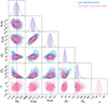 |
Fig. G.1. Fitting results obtained using the Galilean-transformed power spectrum models (pink histograms and 2D contour plots). The blue counterparts illustrate the results derived without the transformation (the same as Fig.11). |
Appendix H: Deriving the estimator of power spectrum and the window function convolution matrix
Corresponding to Sects. 3.2 and 4.3, in this section, we present a detailed derivation of the estimator for the power spectrum and its associated window function convolution matrix by taking the cross-power spectrum as a representative example. The mathematical framework primarily draws upon Sect. 3.1 of Paper I, Sect. 3.2 of Paper III, and Sect. 2.2 of Blake et al. (2018).
H.1. Power spectrum estimator
We begin by introducing the Legendre transformation, denoted as (Blake et al. 2018)
 (H.1)
(H.1)
Following the methodology outlined in Yamamoto et al. (2006) and Sect. 3.2 of Paper III and employing the Fourier transform definition given in Eq. 10, we formulate our estimator for the cross-power spectrum under the "local plane-parallel approximation", i.e.  , as
, as
![Mathematical equation: $$ \begin{aligned} |F^{\delta }(k)F^{p *}_{\ell }(k)|=&\frac{1}{V}\int F^{\delta }(\mathbf{r})e^{i \mathbf{k} \cdot \mathbf{r}} d^3r\frac{1}{V^{\prime }} \int \Big [(2\ell +1)\int F^{p*}(\mathbf{r}^{\prime })L^*_{\ell }(\hat{\mathbf{k}}\cdot \hat{\mathbf{r}^{\prime }})\frac{d \Omega _k}{4\pi }\Big ]e^{-i \mathbf{k} \cdot \mathbf{r}^{\prime }}d^3r^{\prime } \nonumber \\ =&\frac{2\ell +1}{VV^{\prime }}\int \frac{d \Omega _k}{4\pi }\int d^3r \int d^3r^{\prime } F^{\delta }(\mathbf{r})F^{p*}(\mathbf{r}^{\prime }) L^*_{\ell }(\hat{\mathbf{k}}\cdot \hat{\mathbf{r}^{\prime }}) e^{i \mathbf{k} \cdot (\mathbf{r}-\mathbf{r}^{\prime }) }. \end{aligned} $$](/articles/aa/full_html/2026/04/aa58368-25/aa58368-25-eq170.gif) (H.2)
(H.2)
Subsequently, the cross-correlation between the density and momentum fields is expressed as
 (H.3)
(H.3)
Building upon the methodology outlined in Sect. 3.2 of Paper III, and employing Eq. 6 and 8, we derive the cross-correlation between the density and momentum fields as
![Mathematical equation: $$ \begin{aligned} \langle F^{\delta }(\mathbf{r}) F^{p*}(\mathbf{r}^{\prime } ) \rangle =\bigg \langle \frac{w_{\delta }(\mathbf{r})\left[ n_{\delta }(\mathbf{r})-\alpha n_s(\mathbf{r}) \right]}{A_{\delta }}\ \frac{w_p(\mathbf{r}^{\prime })n_p(\mathbf{r}^{\prime })v(\mathbf{r}^{\prime })}{A_p} \bigg \rangle = \frac{1}{ {A_{\delta }A_{p}}} w_{\delta }(\mathbf{r})w_{p}(\mathbf{r}^{\prime })\Big (\langle n_{\delta }(\mathbf{r}) n_p(\mathbf{r}^{\prime } ) v(\mathbf{r}^{\prime } ) \rangle -\alpha \langle n_s(\mathbf{r}) n_p(\mathbf{r}^{\prime } ) v(\mathbf{r}^{\prime } ) \rangle \Big ) \end{aligned} $$](/articles/aa/full_html/2026/04/aa58368-25/aa58368-25-eq172.gif) (H.4)
(H.4)
Drawing from the approach described in Park & Park 2006 and Paper I, the first term within the brackets of Eq. H.4 can be rewritten as  . Given that the cross-correlation between galaxies and random points is zero, the second term within the brackets of Eq. H.4 becomes zero, i.e. α⟨ns(r)np(r′)v(r′)⟩ = 0. Consequently, we obtain
![Mathematical equation: $$ \begin{aligned} \langle F^{\delta }(\mathbf{r}) F^{p*}(\mathbf{r}^{\prime } ) \rangle = \frac{1}{ {A_{\delta }A_{p}}} w_{\delta }(\mathbf{r})w_{p}(\mathbf{r}^{\prime })\big [ \bar{n}_{\delta }(\mathbf{r})\bar{n}_p(\mathbf{r}^{\prime })\xi _{\delta p}(|\mathbf{r}-\mathbf{r}^{\prime }|) + \min \{\bar{n}_{\delta }(\mathbf{r}),\bar{n}_p(\mathbf{r})\} \langle v(\mathbf{r}^{\prime }) \rangle \delta ^D(|\mathbf{r}-\mathbf{r}^{\prime }|)\big ] \end{aligned} $$](/articles/aa/full_html/2026/04/aa58368-25/aa58368-25-eq174.gif) (H.5)
(H.5)
By substituting the above equation into Eq. H.3 in place of ⟨Fδ(r)Fp*(r′)⟩, we arrive at
![Mathematical equation: $$ \begin{aligned} \langle |F^{\delta }(k)F^{p *}_{\ell }(k)|\rangle =&\frac{1}{ {A_{\delta }A_{p}}} \frac{2\ell +1}{V}\int \frac{d \Omega _k}{4\pi }\int d^3r \Big [\frac{1}{V^{\prime }}\int d^3r^{\prime } w_{\delta }(\mathbf{r})w_{p}(\mathbf{r}^{\prime })\bar{n}_{\delta }(\mathbf{r})\bar{n}_p(\mathbf{r}^{\prime })\xi _{\delta p}(|\mathbf{r}-\mathbf{r}^{\prime }|) L^*_{\ell }(\hat{\mathbf{k}}\cdot \hat{\mathbf{r}^{\prime }}) e^{i \mathbf{k} \cdot (\mathbf{r}-\mathbf{r}^{\prime })} \nonumber \\&+ \frac{1}{V^{\prime }} \int d^3r^{\prime }w_{\delta }(\mathbf{r})w_{p}(\mathbf{r})\min \{\bar{n}_{\delta }(\mathbf{r}),\bar{n}_p(\mathbf{r})\} \langle v(\mathbf{r}) \rangle \delta ^D(\mathbf{r}-\mathbf{r}^{\prime }) L^*_{\ell }(\hat{\mathbf{k}}\cdot \hat{\mathbf{r}^{\prime }}) e^{i \mathbf{k} \cdot (\mathbf{r}-\mathbf{r}^{\prime }) }\Big ] \end{aligned} $$](/articles/aa/full_html/2026/04/aa58368-25/aa58368-25-eq175.gif) (H.6)
(H.6)
Upon integrating the second term over the Dirac delta function about r′ using the relation  , we obtain
![Mathematical equation: $$ \begin{aligned} \langle |F^{\delta }(k)F^{p *}_{\ell }(k)|\rangle =&\frac{1}{ {A_{\delta }A_{p}}} \frac{2\ell +1}{V}\int \frac{d \Omega _k}{4\pi }\int d^3r \Big [\frac{1}{V^{\prime }}\int d^3r^{\prime } w_{\delta }(\mathbf{r})w_{p}(\mathbf{r}^{\prime })\bar{n}_{\delta }(\mathbf{r})\bar{n}_p(\mathbf{r}^{\prime })\xi _{\delta p}(|\mathbf{r}-\mathbf{r}^{\prime }|) L^*_{\ell }(\hat{\mathbf{k}}\cdot \hat{\mathbf{r}^{\prime }}) e^{i \mathbf{k} \cdot (\mathbf{r}-\mathbf{r}^{\prime }) }\nonumber \\&+ w_{\delta }(\mathbf{r})w_{p}(\mathbf{r})\min \{\bar{n}_{\delta }(\mathbf{r}),\bar{n}_p(\mathbf{r})\} \langle v(\mathbf{r}) \rangle L^*_{\ell }(\hat{\mathbf{k}}\cdot \hat{\mathbf{r}}) \Big ]\nonumber \\ =&\frac{1}{ {A_{\delta }A_{p}}} \frac{2\ell +1}{V}\int \frac{d \Omega _k}{4\pi }\bigg [\int d^3r \frac{1}{V^{\prime }}\int d^3r^{\prime } w_{\delta }(\mathbf{r})w_{p}(\mathbf{r}^{\prime })\bar{n}_{\delta }(\mathbf{r})\bar{n}_p(\mathbf{r}^{\prime })\xi _{\delta p}(|\mathbf{r}-\mathbf{r}^{\prime }|) L^*_{\ell }(\hat{\mathbf{k}}\cdot \hat{\mathbf{r}^{\prime }}) e^{i \mathbf{k} \cdot (\mathbf{r}-\mathbf{r}^{\prime }) }\nonumber \\&+ \int w_{\delta }(\mathbf{r})w_{p}(\mathbf{r})\min \{\bar{n}_{\delta }(\mathbf{r}),\bar{n}_p(\mathbf{r})\} \langle v(\mathbf{r}) \rangle L^*_{\ell }(\hat{\mathbf{k}}\cdot \hat{\mathbf{r}}) d^3r \bigg ] \end{aligned} $$](/articles/aa/full_html/2026/04/aa58368-25/aa58368-25-eq177.gif) (H.7)
(H.7)
We define the function
 (H.8)
(H.8)
where the shot-noise term  is formally introduced as Eq. 18 of this paper, allowing us to simplify Eq. H.7 into
![Mathematical equation: $$ \begin{aligned} \langle |F^{\delta }(k)F^{p *}_{\ell }(k)|\rangle =\frac{1}{ {A_{\delta }A_{p}}} \frac{2\ell +1}{V}\int \frac{d \Omega _k}{4\pi }\Big [\int d^3r \frac{1}{V^{\prime }}\int d^3r^{\prime } w_{\delta }(\mathbf{r})w_{p}(\mathbf{r}^{\prime })\bar{n}_{\delta }(\mathbf{r})\bar{n}_p(\mathbf{r}^{\prime })\xi _{\delta p}(|\mathbf{r}-\mathbf{r}^{\prime }|) L^*_{\ell }(\hat{\mathbf{k}}\cdot \hat{\mathbf{r}^{\prime }}) e^{i \mathbf{k} \cdot (\mathbf{r}-\mathbf{r}^{\prime }) } + N^{\delta p} \Big ] \end{aligned} $$](/articles/aa/full_html/2026/04/aa58368-25/aa58368-25-eq180.gif) (H.9)
(H.9)
The two-point correlation function maintains an intrinsic relationship with the power spectrum through
 (H.10)
Incorporating this relationship into Eq. H.9 to substitute ξδp leads to
![Mathematical equation: $$ \begin{aligned}&\langle |F^{\delta }(k)F^{p *}_{\ell }(k)|\rangle \nonumber \\ =&\frac{1}{ {A_{\delta }A_{p}}} \frac{2\ell +1}{V}\int \frac{d \Omega _k}{4\pi }\Big [\int d^3r \frac{1}{V^{\prime }}\int d^3r^{\prime } w_{\delta }(\mathbf{r})w_{p}(\mathbf{r}^{\prime })\bar{n}_{\delta }(\mathbf{r})\bar{n}_p(\mathbf{r}^{\prime }) \Big ( \int P^{\delta p}(\mathbf{k}^{\prime })e^{-i \mathbf{k}^{\prime } \cdot (\mathbf{r}-\mathbf{r}^{\prime }) } \frac{d^3k^{\prime }}{(2\pi )^3} \Big ) L^*_{\ell }(\hat{\mathbf{k}}\cdot \hat{\mathbf{r}^{\prime }}) e^{i \mathbf{k} \cdot (\mathbf{r}-\mathbf{r}^{\prime }) } + N^{\delta p} \Big ]\nonumber \\ =&\frac{1}{ {A_{\delta }A_{p}}} \frac{2\ell +1}{V}\int \frac{d \Omega _k}{4\pi }\Big [\Big (\int w_{\delta }(\mathbf{r})\bar{n}_{\delta }(\mathbf{r}) e^{i (\mathbf{k}-\mathbf{k}^{\prime })\cdot \mathbf{r} } d^3r \Big )\frac{1}{V^{\prime }}\int d^3r^{\prime } \int \frac{d^3k^{\prime }}{(2\pi )^3} P^{\delta p}(\mathbf{k}^{\prime }) L^*_{\ell }(\hat{\mathbf{k}}\cdot \hat{\mathbf{r}^{\prime }}) e^{-i (\mathbf{k}-\mathbf{k}^{\prime })\cdot \mathbf{r}^{\prime } }w_{p}(\mathbf{r}^{\prime })\bar{n}_p(\mathbf{r}^{\prime }) + N^{\delta p} \Big ] \end{aligned} $$](/articles/aa/full_html/2026/04/aa58368-25/aa58368-25-eq182.gif) (H.11)
(H.11)
We define the function
 (H.12)
as proposed in Eq. 51, Eq. H.11 can be reduced to
![Mathematical equation: $$ \begin{aligned} \langle |F^{\delta }(k)F^{p *}_{\ell }(k)|\rangle =\frac{1}{ {A_{\delta }A_{p}}} \frac{2\ell +1}{V}\int \frac{d \Omega _k}{4\pi } \Big [ \frac{1}{V^{\prime }}\int d^3r^{\prime } \int \frac{d^3k^{\prime }}{(2\pi )^3} P^{\delta p}(\mathbf{k}^{\prime }) L^*_{\ell }(\hat{\mathbf{k}}\cdot \hat{\mathbf{r}^{\prime }}) e^{-i (\mathbf{k}-\mathbf{k}^{\prime })\cdot \mathbf{r}^{\prime } } w_{p}(\mathbf{r}^{\prime })\bar{n}_p(\mathbf{r}^{\prime }) G^{\delta }(\mathbf{k}-\mathbf{k}^{\prime })+ N^{\delta p} \Big ] \end{aligned} $$](/articles/aa/full_html/2026/04/aa58368-25/aa58368-25-eq184.gif) (H.13)
(H.13)
Expanding the power spectrum Pδp(k′) in terms of Legendre polynomials using Eq. 12 of this paper, we derive
![Mathematical equation: $$ \begin{aligned}&\langle |F^{\delta }(k)F^{p *}_{\ell }(k)|\rangle \nonumber \\ =&\frac{1}{ {A_{\delta }A_{p}}} \frac{2\ell +1}{V}\int \frac{d \Omega _k}{4\pi } \Big [\frac{1}{V^{\prime }} \int d^3r^{\prime } \int \frac{d^3k^{\prime }}{(2\pi )^3} \Big (\sum _{\ell ^{\prime }}P^{\delta p}_{\ell ^{\prime }}(k^{\prime } )L_{\ell ^{\prime }}(\hat{\mathbf{k}}^{\prime }\cdot \hat{\mathbf{r}^{\prime }})\Big ) L^*_{\ell }(\hat{\mathbf{k}}\cdot \hat{\mathbf{r}^{\prime }}) e^{-i (\mathbf{k}-\mathbf{k}^{\prime })\cdot \mathbf{r}^{\prime } } w_{p}(\mathbf{r}^{\prime })\bar{n}_p(\mathbf{r}^{\prime }) G^{\delta }(\mathbf{k}-\mathbf{k}^{\prime })+ N^{\delta p} \Big ]\nonumber \\ =&\frac{2\ell +1}{ {A_{\delta }A_{p}}V} \int \frac{d \Omega _k}{4\pi } \bigg [ \sum _{\ell ^{\prime }} \int \frac{d^3k^{\prime }}{(2\pi )^3} P^{\delta p}_{\ell ^{\prime }}(k^{\prime } ) G^{\delta }(\mathbf{k}-\mathbf{k}^{\prime }) \Big (\frac{1}{V^{\prime }}\int d^3r^{\prime } w_{p}(\mathbf{r}^{\prime })\bar{n}_p(\mathbf{r}^{\prime }) L_{\ell ^{\prime }}(\hat{\mathbf{k}}^{\prime }\cdot \hat{\mathbf{r}^{\prime }}) L^*_{\ell }(\hat{\mathbf{k}}\cdot \hat{\mathbf{r}^{\prime }}) e^{-i (\mathbf{k}-\mathbf{k}^{\prime })\cdot \mathbf{r}^{\prime } } \Big )+ N^{\delta p} \bigg ] \end{aligned} $$](/articles/aa/full_html/2026/04/aa58368-25/aa58368-25-eq185.gif) (H.14)
(H.14)
Further defining the function
 (H.15)
the conjugate form of the above equation enables us to reformulate Eq. H.14 as
![Mathematical equation: $$ \begin{aligned} \langle |F^{\delta }(k)F^{p *}_{\ell }(k)|\rangle =\frac{2\ell +1}{ {A_{\delta }A_{p}}V} \int \frac{d \Omega _k}{4\pi } \Big [ \sum _{\ell ^{\prime }} \int \frac{d^3k^{\prime }}{(2\pi )^3} P^{\delta p}_{\ell ^{\prime }}(k^{\prime } ) G^{\delta }(\mathbf{k}-\mathbf{k}^{\prime }) S^{p*}_{\ell \ell ^{\prime }}(\mathbf{k},\mathbf{k}^{\prime }) + N^{\delta p} \Big ] \end{aligned} $$](/articles/aa/full_html/2026/04/aa58368-25/aa58368-25-eq187.gif) (H.16)
(H.16)
which is similar to Equation 15 of Paper III8. We define the window function as
![Mathematical equation: $$ \begin{aligned} \mathbf{W} \equiv \frac{2\ell +1}{ {A_{\delta }A_{p}}V} \int \frac{d \Omega _k}{4\pi } \Big [ \sum _{\ell ^{\prime }} \int \frac{d^3k^{\prime }}{(2\pi )^3} G^{\delta }(\mathbf{k}-\mathbf{k}^{\prime }) S^{p*}_{\ell \ell ^{\prime }}(\mathbf{k},\mathbf{k}^{\prime }) \Big ] \end{aligned} $$](/articles/aa/full_html/2026/04/aa58368-25/aa58368-25-eq188.gif) (H.17)
(H.17)
in the absence of this component, Eq. H.16 collapses to
 (H.18)
i.e. we can formally express our estimator of the density-momentum cross power spectrum as  with
with  given by Eq. H.2. Consequently, we re-formulate our estimator as
 (H.19)
ensuring its symmetry under  as established in Appendix B.
H.2. Window function
We can expand the Legendre functions in terms of spherical harmonics following the approach outlined in Blake et al. (2018)
 (H.20)
Substituting this expansion and its conjugate into Eq. H.15 yields
 (H.21)
where  is defined by Eq. 50 of this paper. Substituting this result back into Eq. H.17 leads to
![Mathematical equation: $$ \begin{aligned} \mathbf{W} =\frac{1}{ {A_{\delta }A_{p}}} \int \frac{d \Omega _k}{4\pi } \sum ^{\ell }_{m=-\ell }Y^{\ell }_{m}(\hat{\mathbf{k}}) \sum _{\ell ^{\prime }}\frac{(4\pi )^2}{2\ell ^{\prime }+1} \sum ^{\ell ^{\prime }}_{m^{\prime }=-\ell ^{\prime }}\Big [ \frac{1}{V} \int \frac{d^3k^{\prime }}{(2\pi )^3} Y^{\ell ^{\prime }*}_{m^{\prime }}(\hat{\mathbf{k}}^{\prime }) G^{\delta }(\mathbf{k}-\mathbf{k}^{\prime }) \tilde{S}^{p,\ \ell \ell ^{\prime } *}_{mm^{\prime }}( \mathbf{k} ) \Big ] \end{aligned} $$](/articles/aa/full_html/2026/04/aa58368-25/aa58368-25-eq197.gif) (H.22)
(H.22)
which corresponds to Eq. 48 of this paper, and serves as the foundation for computing the window function convolution matrix. The aforementioned expression of W corresponds to the term  . However, as suggested by Blake et al. (2018), in order to derive the corresponding W that conforms to the format specified in Eq. H.19, we just need to substitute the term
  in the above equation with Eq. 53. Notably, the factor V in Equation 19 of Blake et al. (2018) (and Equation 38 of Paper III) is differ from the above Eq. H.22 due to their definition of Fourier transformation and Gδ diverges from our definition presented in Eq. 10 and 51.
H.3. The expression of multipoles
To illustrate the methodology for computing Eq. 20 to 24, we consider the ℓ = 4 auto-power spectrum as a representative example for computing the estimators defined in Eq. 22. In this specific case, Eq. H.2 simplifies to
 (H.23)
By applying Eq. 10, the resulting expression becomes
![Mathematical equation: $$ \begin{aligned}&|F(k)F^{*}_4(k)| \nonumber \\ =&\frac{9}{8}\int \frac{d \Omega _k}{4\pi }F(\mathbf{k})\frac{1}{V^{\prime }} \int d^3r^{\prime } F^{*}(\mathbf{r}^{\prime }) \Big (35 (\hat{\mathbf{k}}\cdot \hat{\mathbf{r}^{\prime }})^4-30 (\hat{\mathbf{k}}\cdot \hat{\mathbf{r}^{\prime }})^2+3 (\hat{\mathbf{k}}\cdot \hat{\mathbf{r}^{\prime }})^0\Big ) e^{-i \mathbf{k} \cdot \mathbf{r}^{\prime } }\nonumber \\ =&\frac{9}{8V^{\prime }}\int \frac{d \Omega _k}{4\pi }F(\mathbf{k}) \bigg [35\int (\hat{\mathbf{k}}\cdot \hat{\mathbf{r}^{\prime }})^4F^{*}(\mathbf{r}^{\prime })e^{-i \mathbf{k} \cdot \mathbf{r}^{\prime } }d^3r^{\prime }-30\int (\hat{\mathbf{k}}\cdot \hat{\mathbf{r}^{\prime }})^2F^{*}(\mathbf{r}^{\prime })e^{-i \mathbf{k} \cdot \mathbf{r}^{\prime } }d^3r^{\prime }+3 \int (\hat{\mathbf{k}}\cdot \hat{\mathbf{r}^{\prime }})^0F^{*}(\mathbf{r}^{\prime }) e^{-i \mathbf{k} \cdot \mathbf{r}^{\prime } }d^3r^{\prime }\bigg ] \end{aligned} $$](/articles/aa/full_html/2026/04/aa58368-25/aa58368-25-eq201.gif) (H.24)
(H.24)
Further incorporating the conjugate form of Eq. 19 for the cases where ℓ = 0, 2, 4, this expression reduces to
![Mathematical equation: $$ \begin{aligned} |F(k)F^{*}_4(k)| =\frac{9}{8V^{\prime }}\int \frac{d \Omega _k}{4\pi }F(\mathbf{k}) [35T^*_4(\mathbf{k})-30 T^*_2(\mathbf{k})+3T^*_0(\mathbf{k})] \end{aligned} $$](/articles/aa/full_html/2026/04/aa58368-25/aa58368-25-eq202.gif) (H.25)
(H.25)
Substituting this expansion into Eq. 13 or Eq. 14 yields
![Mathematical equation: $$ \begin{aligned} P_{4}(k) = \frac{9}{8V^{\prime }}\int \frac{d \Omega _k}{4\pi }F(\mathbf{k}) [35T^*_4(\mathbf{k})-30 T^*_2(\mathbf{k})+3T^*_0(\mathbf{k})]-\fancyscript {N}_{4} \end{aligned} $$](/articles/aa/full_html/2026/04/aa58368-25/aa58368-25-eq203.gif) (H.26)
(H.26)
with 𝒩4 ≈ 0, the above equation collapses precisely to Eq. 22.
All Tables
All Figures
|
Fig. 1. Sky coverage in equatorial co-ordinates of the galaxies analysed within this study. The black dots delineate the sky distribution of BGS galaxies, the grey dots represent that of FP galaxies, and the blue dots illustrate the distribution of TF galaxies. The purple band signifies the galactic plane. |
| In the text | |
|
Fig. 2. Redshift distribution of the galaxies employed in this paper. The y axis is presented on logarithmic scales to enhance the clarity of the data. The black bars depict the redshift distribution of the BGS galaxies, the grey bars delineate the redshift distribution of FP galaxies, and the blue bars illustrate the redshift distribution of TF galaxies. Additionally, the yellow bars represent the redshift distribution of the entire DESI-PV sample, which constitutes a combination of FP and TF galaxies. |
| In the text | |
|
Fig. 3. Galaxy mean number density, denoted as |
| In the text | |
|
Fig. 4. Window function convolution matrix. The horizontal axis is presented on logarithmic scales to enhance the clarity of the data. The left panel displays the convolution matrix for the density power spectrum of the BGS data. The middle panel illustrates the convolution matrix for the momentum power spectrum of the DESI-PV data. The right panel exhibits the convolution matrix for the cross power spectrum between the BGS and DESI-PV data. |
| In the text | |
|
Fig. 5. Window function-convolved model power spectrum computed with different ℓmax values. The parameters of the power spectrum models are taken from Table 2. |
| In the text | |
|
Fig. 6. Power spectrum and parameter fitting outcomes from the BGS and DESI-PV mocks. In the left panels, the filled circles represent the averaged measurements of the density monopole, density quadrupole, momentum monopole, and cross dipole power spectrum, respectively, across 675 mocks. The error bars reflect the uncertainty associated with a single realization. The fitted model power spectrum is overlaid as curves. On the right, the marginalized histograms and two-dimensional contours of the MCMC samples for the cosmological parameters are shown, with the MCMC fit results annotated at the top of each histogram (or see Table 2). The 2D contours delineate the 1, 1.5, 2, and 2.5σ confidence levels, while the shaded regions in the histograms indicate the 1σ confidence interval. The vertical dashed line marks the fiducial value fσ8 = 0.466. |
| In the text | |
|
Fig. 7. fσ8 fit results (represented by filled squares in the top panel) from 15 randomly selected BGS mocks and their corresponding DESI-PV mock counterparts. In the top panel, the dashed yellow line indicates the fiducial value fσ8 = 0.466 of mocks. The blue band represents the fσ8 value from Table 2. The bottom panel illustrates the reduced χ2 values for each measurement, depicted by filled green circles. |
| In the text | |
|
Fig. 8. fσ8 as a function of the cut-off wave number. The filled blue squares show the estimated fσ8 as a function of the cut-off wave number, kmax. The dashed pink line is the fiducial value 0.466. |
| In the text | |
|
Fig. 9. Comparison of the momentum power spectrum derived from the FP data (represented by filled magenta circles) with the averaged spectrum obtained from FP mocks (illustrated by filled blue circles accompanied by error bars). |
| In the text | |
|
Fig. 10. In the top panel, the filled blue squares show the estimated growth rate, fσ8, as a function of the cut-off wave number, kmaxp, of the momentum power spectrum. We fixed kmax = 0.3 h Mpc−1 for the density and cross power spectrum. They were derived from the BGS and DESI-PV survey data. The dashed magenta line indicates the average of the filled blue squares. The dashed yellow line indicates the fiducial value fσ8 = 0.466 of mocks. The bottom panel illustrates the reduced χ2 values for each measurement, depicted by filled green circles. |
| In the text | |
|
Fig. 11. Same as Fig. 6 but for the BGS data and DESI-PV data. In the right panel, the vertical dashed line marks the GR+Planck Collaboration VI (2020) prediction fσ8 = 0.446. The corresponding marginalized parameter values are summarized in Table 3. |
| In the text | |
|
Fig. 12. Constraints on (γ, Ωm, σ8). DESI DR1 (SF+BAO; blue) and its combination with PV consensus fσ8 (orange). Shaded regions show 68% and 95% credible contours. The vertical dashed line marks the GR prediction γ = 0.55. |
| In the text | |
|
Fig. 13. Growth rate, fσ8, as a function of redshift, z. The blue curve represents the theoretical prediction derived under the assumption of GR (γ = 0.55) and a ΛCDM cosmology calibrated using Planck Collaboration VI (2020). The filled green circle denotes the measurement obtained in this study. The filled orange square corresponds to the result from Lai et al. (2025, using MLE), based on the same dataset, while the filled blue pentagon reflects the measurement from Turner et al. (2025, using correlation functions), also utilizing identical data. The filled red diamond corresponds to the consensus result of these three measurements. Additional observational constraints are illustrated by purple circles (using power spectrum), purple squares (using MLE), a purple cross (using reconstruction), and purple pentagons (using correlation functions), representing measurements from other surveys. The light blue pentagrams corresponds to the results from DESI DR1. The dashed orange curve indicates the model fits to all the data points, with the shaded orange region depicting the associated uncertainties. |
| In the text | |
|
Fig. C.1. Linear matter power spectrum PL(k). |
| In the text | |
|
Fig. C.2. Comparing the Kaiser formulas (filled circles), Eqs. C.1, C.2, and C.3 to the linearized perturbation models (curves) Eqs. 29, 30, and 31. |
| In the text | |
|
Fig. C.3. Two-point correlation function models are derived from the power spectrum models introduced in Sect. 4, using the parameter values listed in Table 2. The top panel illustrates the galaxy auto-two-point correlation function |
| In the text | |
|
Fig. E.1. Fitting results obtained with |
| In the text | |
|
Fig. F.1. Same as Fig. 6 but for including the momentum power spectrum quadrupole P2p in the fitting. |
| In the text | |
|
Fig. F.2. Same as Fig. 6 but for including the momentum power spectrum quadrupole P2p in the fitting. The corresponding marginalized parameter values are summarized in Table F.1. |
| In the text | |
|
Fig. G.1. Fitting results obtained using the Galilean-transformed power spectrum models (pink histograms and 2D contour plots). The blue counterparts illustrate the results derived without the transformation (the same as Fig.11). |
| In the text | |
Current usage metrics show cumulative count of Article Views (full-text article views including HTML views, PDF and ePub downloads, according to the available data) and Abstracts Views on Vision4Press platform.
Data correspond to usage on the plateform after 2015. The current usage metrics is available 48-96 hours after online publication and is updated daily on week days.
Initial download of the metrics may take a while.