| Issue |
A&A
Volume 708, April 2026
|
|
|---|---|---|
| Article Number | A11 | |
| Number of page(s) | 13 | |
| Section | Interstellar and circumstellar matter | |
| DOI | https://doi.org/10.1051/0004-6361/202558460 | |
| Published online | 31 March 2026 | |
Diverse stages of star formation in the IRAS 18162-2048 region
Emergence of UV feedback
1
Instituto de Astrofísica de Andalucía, CSIC,
Glorieta de la Astronomía s/n,
18008
Granada,
Spain
2
INAF, Osservatorio Astronomico di Capodimonte,
Salita Moiariello 16,
80131
Napoli,
Italy
3
Departament de Física Quàntica i Astrofísica (FQA), Universitat de Barcelona (UB),
c/ Martí i Franquès 1,
08028
Barcelona,
Spain
4
Institut de Ciències del Cosmos (ICCUB), Universitat de Barcelona (UB),
c/ Martí i Franquès 1,
08028
Barcelona,
Spain
5
Thüringer Landessternwarte Tautenburg,
Sternwarte 5,
07778
Tautenburg,
Germany
6
Instituto de Astronomía Teórica y Experimental (IATE), Universidad Nacional de Córdoba (UNC),
Córdoba,
Argentina
7
Instituto de Radioastronomía y Astrofísica, Universidad Nacional Autónoma de México,
Morelia,
Michoacán
58089,
Mexico
8
INAF, Osservatorio Astronomico di Cagliari,
via della Scienza 5,
09047
Selargius,
Italy
9
INAF, Osservatorio Astrofisico di Arcetri,
Largo E. Fermi 5,
50125
Firenze,
Italy
10
Dublin Institute for Advanced Studies, School of Cosmic Physics,
31 Fitzwilliam Place,
Dublin 2,
Ireland
11
University College Dublin, School of Physics,
Belfield,
Dublin 4,
Ireland
12
Jodrell Bank Centre for Astrophysics, Department of Physics & Astronomy, The University of Manchester,
Oxford Road,
Manchester
M13 9PL,
UK
13
I. Physikalisches Institut, Universität zu Köln,
Zülpicher Str 77,
50937
Köln,
Germany
★ Corresponding author: This email address is being protected from spambots. You need JavaScript enabled to view it.
Received:
8
December
2025
Accepted:
9
February
2026
Abstract
Context. High-mass star formation remains a major open problem in astrophysics, particularly regarding the transition between deeply embedded protostars and the onset of ionising radiation capable of producing photodissociation regions (PDRs) and compact H II regions.
Aims. We aim to characterise the excitation and ionisation conditions of the high-mass star-forming region IRAS 18162−2048, which is where the parsec-scale jet HH80−81 lies.
Methods. We obtained adaptive optics–assisted integral field spectroscopy in the near-IR K band (1.93–2.47 µm) with VLT/SINFONI, complemented by VLA X and C bands (3−6 cm) and ALMA band 3 (∼3.3 mm) observations. We analysed the continuum and line emission to derive visual extinction and excitation conditions and the kinematics of the gas of the region.
Results. The near-IR continuum reveals two IR sources, IRS 2 and IRS 7, while the main protostellar core, IRAS 18162-2048, remains undetected up to 2.47 µm. IRS 7 shows a peculiar hydrogen recombination line (HRL) Brγ profile with a narrow emission component superimposed on a broad absorption feature, consistent with a B2/B3 zero-age main-sequence (ZAMS) star. Extended H2 emission exhibits a ‘sawtooth’ pattern in the excitation diagram, characteristic of UV radiation in a PDR rather than shock excitation. The radiative transfer model Cloudy reproduces the H2 ro-vibrational populations for Tgas = 600 K and nH = 7.9 × 103 cm−3. The VLA X and C bands observations reveal a compact radio source previously reported as a ‘stationary condensation’ (SC) and coincident with IRS 7. For the first time, we detect IRS 7/SC in millimetre wavelengths. The spectral index in the 3−6 cm and 3.3 mm regime is consistent with optically thin free–free emission.
Conclusions. Our near-IR and radio observations reveal that IRS 7/SC is a B2/B3 ZAMS star that has begun to photo-ionise its environment, giving rise to an extended PDR and a compact H II region. The coexistence of this source with the deeply embedded protostar IRAS 18162-2048 and other bubble-like structures in the field suggests a multi-generational star-forming environment. Future James Webb Space Telescope observations targeting the H2 pure rotational lines (3–28 µm) and other HRLs less affected by extinction will be essential to characterising the cooler molecular and ionised gas to fully disclose the formation history of the region.
Key words: stars: formation / stars: individual: IRAS 18162-2048 / ISM: bubbles / HII regions / ISM: individual objects: HH 80-81
© The Authors 2026
 Open Access article, published by EDP Sciences, under the terms of the Creative Commons Attribution License (https://creativecommons.org/licenses/by/4.0), which permits unrestricted use, distribution, and reproduction in any medium, provided the original work is properly cited.
This article is published in open access under the Subscribe to Open model. This email address is being protected from spambots. You need JavaScript enabled to view it. to support open access publication.
1 Introduction
The formation of low-mass (M∗ < 2 M⊙) and high-mass (M∗ > 8 M⊙; Lbol > 103 L⊙) stars has traditionally been studied along separate pathways (e.g. Beuther et al. 2007; Frank et al. 2014; Tan et al. 2014). Yet it is increasingly clear that stars of different masses can form together, evolve on different timescales, and interact dynamically with their common environment (see Beuther et al. 2025, for a review). In such clustered settings, massive (proto-)stars strongly influence their surroundings through a variety of feedback processes, from powerful jets, winds, and outflows to intense UV stellar radiation that rapidly produces compact H II regions. Unlike their low-mass counterparts, massive protostars reach the zero-age main sequence (ZAMS) while still accreting (Palla & Stahler 1993), irradiating, and shaping their natal cloud, even during their earliest growth phases. At the same time, several characteristics of star formation appear to scale smoothly across the mass spectrum, such as the ubiquity of accretion discs (Beltrán & de Wit 2016; Andrews et al. 2018) and associated collimated jets and outflows (Bally 2016; Anglada et al. 2018; Ray & Ferreira 2021).
Feedback from massive stars can disrupt local gas reservoirs, but it also has the potential to induce or accelerate subsequent star formation. Theoretical work and observations over the past decades have pointed towards feedback-driven triggering in bright-rimmed clouds, expanding H II regions, and wind-blown bubbles (e.g. Klein et al. 1980; Sugitani et al. 1989; Elmegreen 2011). In addition, protostellar jets and molecular outflows themselves may compress and destabilize dense gas, seeding the next generation of young stars (e.g. Girart et al. 2001; Osorio et al. 2017). Understanding the interplay between accretion, feedback, and clustered formation, especially in high-mass protostellar regions, therefore remains central to building a complete theory of star formation.
The high-mass star-forming region IRAS 18162-2048 (d ∼ 1.4 kpc, Lbol ∼ 104 L⊙; Añez-López et al. 2020) offers a unique opportunity to investigate these processes in action. Its central main protostar, IRAS 18162-2048, is a deeply embedded 20–30 M⊙ protostar driving the spectacular ∼15 pc (in projection) HH 80–81 multi-wavelength jet (Marti et al. 1993; Carrasco-González et al. 2010; Masqué et al. 2012; Bally & Reipurth 2023; Mohan et al. 2023). The surrounding cluster contains numerous young stellar objects (YSOs) with circumstellar masses (most likely tracing discs) between 0.003 and ∼5 M⊙, identified in high-resolution ALMA band 6 observations (Busquet et al. 2019; Añez-López et al. 2020). Mid-IR imaging (8–13 µm) has also revealed embedded sources such as IRS 2 and IRS 7, which may be more evolved sources (Stecklum et al. 1997). The region therefore presents a hint of multi-generational star formation, where massive proto-stellar accretion, disc-jet activity, and emerging UV-driven photo-ionisation may coexist within a compact environment.
Despite the wealth of existing observations, the region IRAS 18162-2048 continues to pose fundamental questions. The origin of the bright H2 emission, the nature of compact centimetre to millimetre sources in the vicinity of the main protostar, and the degree to which newly formed massive stars irradiate and reshape their environment remain unclear. Further, whether these signatures are solely the result of shock activity from ongoing accretion and outflows or they instead mark the ignition of young OB-type stars and the development of compact H II regions and photodissociation regions (PDRs) is also unknown. To address these questions, we combined near-IR integral field spectroscopy with radio observations to map the molecular and ionised gas with the aim of identifying the emission mechanisms.
The paper is structured as follows: in Sect. 2 we detail the observations taken and the data reduction procedures. In Sect. 3 we present our results, while in Sect. 4 we discuss the implications of our findings. Section 5 contains our conclusions.
2 Observations
2.1 VLT/SINFONI
The Very Large Telescope (VLT) Spectrograph for INtegral Field Observations in the Near-Infrared (SINFONI; Eisenhauer et al. 2003) data were obtained on 3 August 2018 as part of the programme ID 0101.C-0317(A) (PI: R. Fedriani), targeting the first ∼10 000 au of the high-mass star-forming region IRAS 18162-2048. The observations consist of eight AB nodding positions, each with DIT=30 s and NDIT=6 for the science positions and NDIT=3 for the sky positions. Total exposure times of 180 s and 90 s were set per frame for the science and sky positions, respectively. The field of view (FoV) was centred at the IRS 7 source covering 8″ × 8″ (11 200 × 11 200 au2 at a distance of 1.4 kpc) with a spaxel size of 250 mas pixel−1, and the position angle was east of north of zero degrees. The observations were adaptive optics assisted with a natural guide star, reaching an angular resolution of ∼0.6″. The natural guide star used was 2MASS J18191071-2047423 with R = 13.6 mag and B-R colour 0.17, and it was separated from the science target by 20″. We set up the K grating with a spectral resolution of ∼4000 (∼75 km s−1). The data were reduced using the European Southern Observatory pipeline gasgano with standard parameters. A wavelength accuracy of 0.09 Å (i.e. ∼1.3 km s−1) was achieved using arc lamps (neon plus argon in the K band). The standard star Hip 088201 was used for spectral calibration and telluric correction.
2.2 VLA
The radio centimetre continuum emission from the IRAS 18162-2048 region was observed with the Karl G. Jansky Very Large Array (VLA) of the National Radio Astronomy Observatory (NRAO) in A configuration (VLA-A) at C (covering the frequency range 4–8 GHz, i.e. ∼6 cm) and X (covering 8–12 GHz, i.e. ∼3 cm) bands during August 2019 (project code: 19A-321, PI: A.R. Rodríguez-Kamenetzky). The phase centre was set at RA (J2000) = 18h19m12.09s, Dec (J2000) = +20◦47′30.89″.
Data calibration was conducted with the Common Astronomy Software Applications (CASA; version 6.4.1; CASA Team 2022) package using the NRAO pipeline optimised for VLA continuum observations. We adopted the standard frequency setup for the continuum, utilising 2 MHz-wide channels across the full bandwidth of each band. The source 3C 286 served as both the bandpass and flux calibrator, while complex gain calibration (phase and amplitude) was derived from frequent observations of J1911–2006. Calibrated datasets from both bands were concatenated into a single file for subsequent imaging and self-calibration. Imaging was carried out with the tclean task in CASA, employing multi-frequency synthesis (nterms = 2) and multi-scale cleaning algorithms (Rau & Cornwell 2011). Primary beam correction was applied, and super-uniform weighting was used to maximise angular resolution, yielding a restoring beam of 0.30″ × 0.14″ with a position angle of 21.5◦ and a root mean square (rms) noise σ = 7 µJy beam−1.
2.3 ALMA
Observations were carried out with the Atacama Large Millimeter/submillimeter Array (ALMA) in band 3 on 27 June 2014 as part of the program 2012.1.00441.S (PI: R. Galván-Madrid). The source J1733-1304 was used as a flux-scale and bandpass calibrator, and J1832-2039 was used as a gain calibrator. Visibility calibration and imaging were performed with CASA version 5.0.0, using as the phase centre RA (J2000) = 18h19m12.094s, Dec (J2000) = −20◦47′30.91″. The spectral setup included four spectral windows of 0.94 GHz of bandwidth each, centred at 92.03, 92.87, 105.89, and 106.73 GHz. All the line-free channels of these spectral windows were combined to produce the continuum image presented in this paper.
The image has a central frequency of 99.39 GHz (∼3.3 mm), a beamsize of 0.99″ × 0.95″, a position angle of 77.4◦ (Briggs weighting with robust=0.5), and an rms noise σ = 18 µJy beam−1, which was achieved after a few iterations of phase self-calibration.
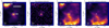 |
Fig. 1 Left: SINFONI K band continuum view of the IRAS 18162-2048 star-forming region. The black and white boxes represent the extraction regions for the spectra shown in Fig. 2. The black crosses represent the positions of IRS 2 and IRS 7 (peak intensity pixel from SINFONI), and the red cross shows the position of IRAS 18162-2048 (from the VLA data). Middle left: peak intensity continuum-subtracted map for the Brγ emission line. The white crosses represent the positions of IRS 2 and IRS 7, and the red cross indicates the position of IRAS 18162-2048. Middle right: peak intensity map for the 1–0 S(1) H2 emission line including the continuum emission. Right: same as middle-right panel but with the continuum subtracted. In all panels, the full FoV of SINFONI is shown. |
3 Results
3.1 Spatial and spectral distribution of the emission in the near-infrared
Our spectro-imaging observations cover the first ∼10 000 au of the IRAS 18162-2048 region. The left panel of Fig. 1 shows the continuum emission constructed using 555 line-free channels across the SINFONI K band spanning 1.93–2.47 µm. We identified two previously reported sources, IRS 2 and IRS 7 (Yamashita et al. 1987; Tamura et al. 1991). The main proto-star IRAS 18162-2048 is not detected at any wavelength within this spectral range, even when summing all continuum channels, indicating a much higher level of extinction toward this source. We observed extended continuum emission around IRS 7, suggesting scattered light in the vicinity. We measured its Ks band magnitude by integrating the flux at 2.159 µm. We first adopted the 2.8″ aperture defined by Stecklum et al. (1997), obtaining Ks = 11.52 ± 0.01 mag, consistent with the value reported at the epoch of March 1995 (∼11.60 mag; see their Table 1). Moreover, 2MASS reports Ks ∼ 11.51 mag at the epoch of 10 June 1999 (Skrutskie et al. 2006). This suggests no major brightening or dimming events have occurred over the past few decades, based on the consistent brightness level across all three measurements, although the intervening activity remains unknown. Using our improved angular resolution, we measured the magnitude in a smaller region of 1″ (central white box in Fig. 1), yielding Ks = 12.79 ± 0.02 mag. No magnitude was estimated for IRS 2, as it lies near the edge of our FoV, and it is clearly not entirely covered in our observations, leading to flux losses.
The middle-right panel of Fig. 1 shows the combined line and continuum emission of the 1–0 S(1) molecular hydrogen (H2) transition at 2.12 µm. The continuum-subtracted H2 emission (Fig. 1, right panel) resembles what is typically associated with protostellar outflows (see e.g. Varricatt et al. 2010; Caratti o Garatti et al. 2015), even displaying a bow-shaped-like feature (see e.g. Fedriani et al. 2018; Ray et al. 2023; Crowe et al. 2024, 2025). However, as discussed in Sect. 3.3, this emission is produced by UV pumping and most likely traces a PDR with a bubble-like structure. Conversely, the hydrogen recombination line (HRL) Brγ at 2.16 µm is detected exclusively towards the position of IRS 7 (see Fig. 1 middle-left panel and Fig. 2 top panel). In star-forming regions, the Brγ line is often used as a tracer of accretion and ejection processes occurring very close to the central protostar (Coffey et al. 2010; Alcalá et al. 2014; Caratti o Garatti et al. 2016). In our case, however, the emission is not spatially extended, or it presents a P-Cygni profile and therefore is unlikely to trace protostellar jets (Davies et al. 2010; Fedriani et al. 2019) or the innermost region of accretion discs given its line profile (GRAVITY Collaboration 2020, 2024), although this depends on the inclination angle. A detailed analysis of the Brγ line profile and its possible origin is presented in Sect. 3.2.
Figure 2 shows the spectra extracted from the regions marked by the black and white boxes in Fig. 1 (left panels). Both IRS 2 and IRS 7 display clear signs of reddening, but it is stronger in IRS 2 (see top panel of Fig. 2). The IRS 2 spectrum shows no prominent emission lines other than the ubiquitous 1–0 S(1) H2 line, which is detected across the entire FoV. Aspin (1994) also found a featureless spectrum for IRS 2. In contrast, the IRS 7 spectrum exhibits numerous H2 transitions, most likely arising from a PDR. There are a number of spurious peaks in the spectra marked with dotted red lines and labelled with ‘+’. It should also be noted that the wiggles in the range 2.0–2.1 µm are noise and not real emission. Notably, the HRL Brγ displays a composite absorption plus emission profile. A close-up view of this feature is provided in Fig. 3. The bottom panel of Fig. 2 presents the rich H2 spectrum extracted from the white south box region shown in the left panels of Fig. 1. Gaussian profiles were fitted to the H2 emission lines, and the fluxes were derived by integrating under the fitted curves. The rms noise was estimated from the continuum surrounding each line to determine the associated flux uncertainties. Table 1 summarises the H2 lines detected within the white south box region, which represents the highest signal-to-noise ratio (S/N) region. For each transition, the table lists the vacuum wavelength, the integrated flux, and the corresponding S/N. Interestingly, nowhere in our cube did we find evidence of additional emission lines that are usually associated with accretion and ejection processes in the circumstellar environment of YSOs, such as [Fe II], Na I, He I, or the CO band head.
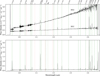 |
Fig. 2 Top: spectra for IRS 2 and IRS 7 as labelled. Bottom: spectrum extracted at the highest S/N in the main region of H2 emission. Extraction boxes are shown in Fig. 1. Main H2 emission lines are marked as vertical dashed green lines, Brγ as a dotted green line, and noisy peaks as dotted red lines and labelled as ‘+’. |
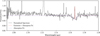 |
Fig. 3 Zoom-in of the IRS 7 spectrum at the 2.07–2.20 µm range. A double Gaussian profile (emission plus absorption) fit to the Brγ line is shown as a dashed red line, whereas the dotted blue line shows the single Gaussian profile fit to the absorption component. Strong emission lines correspond to H2, in particular 2–1 S(3), 1–0 S(1), 3–2 S(4), and 2–1 S(2), at 2.074, 2.122, 2.128, and 2.154 µm, respectively. |
3.2 The hydrogen recombination line Brackett gamma
Line profiles can provide key diagnostics of the physical mechanisms at work in YSOs. For example, inverse P-Cygni profiles (i.e. strong red-shifted continuum absorption) are associated with infalling material in molecular emission at large scales (Zapata et al. 2008), whereas P-Cygni profiles (i.e. strong blue-shifted continuum absorption) are linked to strong ejection activity for ionised winds close to the central sources (Najarro et al. 1997). The Brγ line in YSOs has been observed to trace jets close to the protostar (Caratti o Garatti et al. 2016) and accretion processes within circumstellar discs (GRAVITY Collaboration 2020). A prominent P-Cygni profile was observed in the high-mass YSO IRAS 13481−6124 (Fedriani et al. 2018), where the line traces powerful jets close to the massive protostar. In our case, we detected Brγ emission only at the position of IRS 7, showing a peculiar line profile. The line exhibits a clear emission core superimposed on a broad absorption feature (see Fig. 3). We fitted a double Gaussian profile to the Brγ line, accounting for both the emission and absorption components. The emission component is unresolved at our spectral resolution of ∼75 km s−1 and peaks at ∼0 km s−1 in the local standard of rest. These two facts suggest that it could be tracing an H II region, while the absorption feature displays a full width at half maximum of ∼750 km s−1. Considering only the absorption component, we estimate an equivalent width (EW) of 2.2 ± 0.2 Å. To the best of our knowledge, this is the first detection of an HRL in the region of IRAS 18162-2048.
Notes. Fluxes were measured within the region indicated by the white south box in Fig. 1.
The observed line profile is characteristic of an OB-type ZAMS star. Bik et al. (2005) conducted a high spectral resolution (R ∼ 10 000, corresponding to ∼30 km s−1) survey of deeply embedded young massive star candidates and established that O-and B-type stars can be empirically distinguished by their Brγ EW, with a boundary at EW = 5 Å, and by the presence (or a lack) of a number of emission lines. Although our EW measurement could nominally place IRS 7 in the O-type regime by the classification scheme of Bik et al. (2005), this value may be affected by veiling, which tends to reduce the apparent depth of absorption features. We can confidently rule out an O-type classification for IRS 7, as we did not detect the characteristic C IV lines at 2.069, 2.078, and 2.083 µm; the He I lines at 2.058, 2.112, and 2.113 µm; the N III line at 2.115 µm; nor the He II line at 2.185 µm, all of which were found in the spectra of O-type sources by Bik et al. (2005). We therefore classify IRS 7 as a B2/B3 ZAMS star (see Bik et al. 2005, and references therein for details on the classification scheme). This was confirmed later by our radio observations (see Sect. 3.5).
We interpret the broad absorption component as originating from the stellar photosphere (Bik et al. 2005, found full width at zero intensity of 800 km s−1 for the Brγ for other sources in their survey), while the narrow unresolved emission core most likely traces ionised gas associated with an incipient H II region surrounding IRS 7. This interpretation is consistent with the presence of extended continuum and H2 emission in the vicinity, which together indicate that IRS 7 is already influencing its immediate environment through both radiative and mechanical feedback.
Molecular hydrogen (H2) emission lines detected on IRAS 18162-2048.
3.3 Extinction and excitation conditions
Line ratios involving transitions that originate from the same upper energy level can be used to estimate the extinction along the line of sight (e.g. Nisini 2008). Ideally, these lines should be widely separated in wavelength to maximise sensitivity to reddening. However, our spectral setup covers only the K band, from 1.93 to 2.47 µm. To estimate the visual extinction, AV, we used the H2 1–0 Q(3)/1–0 S(1) line ratio, which offers the highest S/N among the available line pairs. We followed the same approach described by Costa Silva et al. (2022) (but see also Zannese et al. (2025)) and adopted the near-IR extinction law from Rieke & Lebofsky (1985).
Since our data provide spectra for every pixel, we could construct a spatially resolved AV map. Figure 4 (left panel) shows the resulting pixel-by-pixel extinction distribution. For instance, at the position of IRS 2, the 1–0 Q(3) line is not detected with sufficient S/N, leading to unreliable extinction estimates in that region, and therefore it has been masked (grey region in the figure). Across the main H2 bow-shaped structure, the average extinction is ∼12 mag, consistent with the value of 12.4 mag reported by Stecklum et al. (1997) using an independent method. In their method, the authors reddened the blackbody spectrum of a B2 ZAMS star by varying the extinction until the model matched the observed photometry from the R to the K band.
The H2 line ratio 1–0 S(1)/2–1 S(1) provides insights into the excitation mechanism of the emitting gas (Fig. 4 middle panel). For shock excitation, this ratio is expected to exceed ∼10, whereas for purely UV-pumped emission, it is typically ∼1.7 (Burton 1992). After correcting the fluxes for extinction using our derived AV values, we obtained an average ratio of ∼5.9. This clearly indicates that the H2 emission in the region is inconsistent with purely shock-driven thermal excitation and instead points to UV fluorescence as the dominant process (see Sect. 3.4). However, Burton et al. (1990) showed that in dense PDRs, collisional processes can alter the level populations, leading to deviations from those expected for purely UV-excited gas (see also Sternberg & Neufeld 1999). Therefore, we are probably observing an intermediate case between UV-excited and shocked H2. This is more evident in the southeast region of our observations, where the ratio is greater than eight, although with just a few pixels with ratios consistent with shocks (i.e. ≳10).
Velocity maps provide key insight into the kinematics associated with a given emitting species. The right panel of Fig. 4 presents the radial velocity map of the H2 1–0 S(1) line with respect to the systemic velocity of the region, which is the strongest and best isolated transition in our dataset. We used the Python package bettermoments (Teague & Foreman-Mackey 2018) to fit Gaussian profiles to the line emission across the field, considering only pixels with S/N > 3. The average radial velocity within the main emitting region is ∼1 km s−1, indicating negligible bulk motion along the line of sight. It should be noted that although the nominal spectral resolution of our observations is ∆v ∼ 75 km s−1, the centroid velocity of the line can be measured with higher precision, scaling as  . For the H2 1–0 S(1) line, with an average S/N ∼ 100, this corresponds to uncertainties of ∼7.5 km s−1. Even for the pixels with S/N∼3, the uncertainty would be ∼43 km s−1. In any case, such low velocities are consistent with two scenarios: (i) a potential outflow oriented nearly in the plane of the sky, resulting in minimal radial velocity components or (ii) PDR-excited H2 emission. In shock–driven H2 emission associated with protostellar jets, velocity shifts of tens to hundreds of kilometres per second are typically observed (e.g. Fedriani et al. 2018, 2019) and so is evidence of blue- and red-shifted components (e.g. Fedriani et al. 2020). In contrast, PDR–excited H2 usually exhibits very small velocity gradients close to the systemic velocity (Burton et al. 1990; Marconi et al. 1998). Combined with the excitation analysis presented earlier, this velocity structure strongly supports a PDR origin for the observed H2 emission rather than shock-driven outflow activity (see also Sect. 3.4). Together, the extinction, excitation, and velocity maps analyses provide a consistent picture in which UV radiation from nearby massive (proto-)stars plays a key role in shaping the observed near-IR emission.
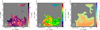 |
Fig. 4 Left: extinction map obtained from the H2 1–0 Q(3)/1–0 S(1) line ratio. Middle: excitation map from the H2 line ratio 1–0 S(1)/2–1 S(1). Right: radial velocity map using the H2 1–0 S(1) line. In all panels, grey indicates masked pixels with S/N < 3. |
3.4 H2 ro-vibrational diagrams
The combined effects of UV radiation and collisional excitation produce two limiting regimes for the ro-vibrational level populations. In dense and/or hot environments, such as shocked gas in protostellar outflows, frequent collisions drive the level populations towards a thermal (Boltzmann) distribution, resulting in ro-vibrational diagrams that follow a straight line in a logarithmic excitation plot (e.g. Caratti o Garatti et al. 2008). In contrast, low-density gas exposed to intense UV radiation exhibits a distinct distribution, with populations that do not decrease monotonically with excitation energy. In excitation diagrams, this manifests as a characteristic ‘sawtooth’ pattern, which serves as a diagnostic signature of UV-pumped H2 emission in PDRs (Burton 1992; Kaplan et al. 2017; Le et al. 2017). Such diagrams provide a clear distinction between collisional and radiative excitation mechanisms and give constraints on both the gas temperature and the ortho-to-para ratio (OPR).
We constructed a ro-vibrational diagram using the de-reddened fluxes from Table 1 corresponding to the white south box, adopting AV = 12 mag. To model the emission, we fitted a two-temperature component while leaving the OPR as a free parameter. A single temperature component fit failed to reproduce the observed H2 intensities. Figure 5 shows the resulting ro-vibrational diagram for the observed H2 lines together with the fit obtained using the PDR Toolbox (Pound & Wolfire 2023). The characteristic ‘sawtooth’ pattern of PDRs is clearly visible, confirming the dominance of UV pumping in the emission, instead of a near-linear thermal distribution. The best-fit model yields a cold component with Tcold ∼ 400 K, a hot component with Thot ∼ 3000 K, a total H2 column density N(H2) ∼ 2 × 1023 cm−2, and an OPR= 2.76 ± 0.14.
The derived hot-component temperature is higher than typically observed in protostellar outflow knots, where values of Thot ∼ 2000 K are more common, and the ro-vibrational diagrams usually follow a near-linear thermal distribution (Caratti o Garatti et al. 2015; Costa Silva et al. 2022). This further supports the conclusion that UV pumping is the dominant excitation mechanism in the H2 emission for which Tcold is a better tracer of the kinetic temperature of the gas. The fitted OPR is 2.76 ± 0.14, which is somewhat high for pure PDR emission (see e.g. Le et al. 2017, and references therein). As mentioned above, we are probably observing an intermediate case between UV- and shocked-excited H2 emission. However, the collective near-IR evidence points towards a strong contribution from UV-pumped excitation.
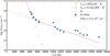 |
Fig. 5 Ro-vibrational diagram using the fluxes extracted from the white south box depicted in Fig. 1 and summarised in Table 1. The blue circles represent the observed H2 data after extinction correction (AV = 12 mag), and the pink line shows the two-temperature component. The plot was generated using the PDR Toolbox (Pound & Wolfire 2023). |
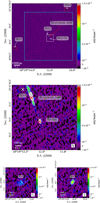 |
Fig. 6 Top: VLA X and C band continuum image. The cyan box represents the field shown in Fig. 7, whereas the white box represents the FoV of SINFONI. The main sources in the region are labelled. Middle: same as above but zoomed in on the SINFONI FoV. Contours are (−3, 3, 5, 10, 15) × σX+C where σX+C = 7µJy beam−1. The red crosses represent the VLA positions for IRAS 18162-2048 and IRS 7/SC, and the white crosses are the SINFONI positions for IRS 2 and IRS 7/S. Bottom: zoomed in views of the red boxes in the top panel highlighting IRS 3 (left) and IRS 4 (right). The synthesised beams are shown at the bottom-right corners. |
3.5 Radio emission at millimetre and centimetre wavelengths
We present new high-sensitivity VLA A-configuration observations at ∼3–6 cm (X and C bands). Figure 6 shows the resulting radio continuum map of the IRAS 18162-2048 region, where several compact sources were clearly detected. In addition to the emission associated with the main protostar IRAS 18162-2048, we also detected a non-resolved compact radio counterpart to IRS 7. Further emission was observed at the positions of the IR sources IRS 3 and IRS 4 originally identified by Yamashita et al. (1987). Both objects were later detected in the radio by Marti et al. (1993), who catalogued them as sources 20 (IRS 3) and 12 (IRS 4) in their Table 2.
Notes. Positional uncertainties are ∼50 mas. The symbols are as follows: a catalogued in Table 1 from IR observations by Yamashita et al. (1987); b catalogued in Table 5 from IR observations by Tamura et al. (1991);† catalogued in Table 2 as sources 12, 13, and 20, respectively, from radio observations by Marti et al. (1993);∗ referred to as stationary condensation (SC) in Marti et al. (1995).
Interestingly, both IRS 3 and IRS 4 are visible in the Hα (6564 Å) image presented in Fig. 1 of Bally & Reipurth (2023), suggesting the presence of ionised material in relatively low-extinction regions. Moreover, each source appears as a point-like object surrounded by bubble-like structures, corresponding to the molecular hydrogen objects (MHOs) 2357 and 2359, respectively (see Figs. 15 and 16 in Bally & Reipurth 2023). A similar identification was made by Mohan et al. (2023), who classified IRS 3 and IRS 4 as ‘YSO2’ and ‘YSO1’, connected to their ‘Reg3’ and ‘Reg5’ regions (see their Fig. 2). IRS 4, in particular, has been proposed to be a Herbig Ae/Be star of spectral type B2, and it is thought to be responsible for carving the prominent H2 bubble observed around it (Bally & Reipurth 2023). We performed 2D Gaussian fits to all compact detections except for the main protostar IRAS 18162-2048 and its jet, as analysis of its complex morphology goes beyond the scope of this paper. Table 2 presents a summary of their positions and flux densities. A discussion of the nature of these sources is provided in Sect. 4.
Figure 7 shows complementary ALMA continuum emission at ∼3.3 mm. We overlayed the ALMA ∼1.14 mm compact sources reported by Busquet et al. (2019) as red crosses. Several objects are detected in both bands, while others are only recovered at one of the ALMA frequencies. This behaviour may result from a combination of dust opacity, differing evolutionary stages, and optical depth effects. We also note the considerable difference in angular resolution and sensitivity between the ALMA ∼1.14 mm data (∼45 mas, ∼56 µJy beam−1; Busquet et al. 2019) and our ∼3.3 mm image (∼1″, ∼18 µJy beam−1), which likely contributes to the observed difference between wavelengths.
A particularly noteworthy result is the detection of IRS 7 in our 3.3 mm data. It is the first time this source has been detected in the millimetre regime. A Gaussian fit to the ALMA band 3 emission of IRS 7 yields S3.3mm = 0.457 ± 0.310 mJy, and it is non-resolved. The source was originally identified in the radio continuum by Marti et al. (1993), who later referred to it as the ‘stationary condensation’ (SC) due to its lack of proper motions, in contrast to the extremely high velocity (∼1000 km s−1) HH 80–81 jet knots (Marti et al. 1995; Bally & Reipurth 2023). IRS 7 was first identified by Tamura et al. (1991) in the IR. Later, Stecklum et al. (1997) associated IRS 7 with the SC, and our detections confirm this identification.
We calculated the spectral index of IRS 7/SC given their non-resolved detections at both centimetre and millimetre wavelengths, defined as
 (1)
(1)
where ν1 = 8.19 GHz and ν2 = 99.3 GHz, corresponding to the observed frequencies for VLA and ALMA, respectively. We obtained a value of α = 0.19 ± 0.27, which is consistent with almost optically thin free-free emission (i.e. −0.1 ≤ α ≤ 2 for free-free emission; Anglada et al. 1998; Purser et al. 2016; Sanna et al. 2018). In fact, assuming that the emission at 3– 6 cm arises from free-free emission, extrapolating with a spectral index of −0.1 (optically thin emission) would provide a strict lower limit to the free-free contribution at higher frequencies. This extrapolation would yield a value of 0.220 ± 0.011 mJy at 3.3 mm, which is what we actually detect within the errors. Moreover, Marti et al. (1995) reported a flat spectral index between 3.6 and 6 cm, consistent with optically thin free-free emission as well. Thus, we can confidently conclude that dust is not the dominant origin of the emission in IRS 7/SC, supporting the interpretation that this source is a compact photo-ionised H II region powered by a B2/B3 ZAMS star (see Sect. 4).
We note that IRS 2 is not detected at either 3–6 cm or 3.3 mm. This applies to our data and to previous studies (e.g. Marti et al. 1993; Rodríguez-Kamenetzky et al. 2017; Busquet et al. 2019). This non–detection may suggest a later evolutionary stage, where accretion and jet activity have declined and no detectable ionised region has developed, or alternatively a lower–luminosity source below our sensitivity threshold. It could also correspond to a non-stellar object, with the observed IR emission arising from scattered light from nearby sources, as suggested by Aspin (1994).
VLA X and C band detections in the region IRAS 18162-2048, excluding the main protostar and its jet.
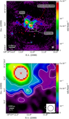 |
Fig. 7 Top: ALMA band 3 (∼3.3 mm) image in the region IRAS 18162-2048. Red crosses are ALMA 1.14 mm detections in the field (Busquet et al. 2019), with the larger cross corresponding to the main protostar IRAS 18162-2048. The large white crosses indicate the positions of IRS 2 and IRS 7/SC from their SINFONI positions. The white box represents the SINFONI FoV. Bottom: same as above but zoomed in on the SINFONI FoV. Contours are (−3, 3, 5, 10, 15) × σ3.3mm, where σ3.3mm = 18 µJy beam−1. The synthesised beams are shown at the bottom right corners. |
4 Discussion
4.1 IRS 7: A B2/B3 zero-age main-sequence star powering an H II and a photodissociation region
Our results strongly indicate the presence of sources of UV photons within the region of IRAS 18162-2048. The Brγ line profile observed towards IRS 7/SC is consistent with that of a B2/B3 ZAMS star (Bik et al. 2005). In addition, the presence of a PDR is revealed by the H2 emission morphology, its kinematics (Fig. 4), and the distinct ro-vibrational ‘sawtooth’ pattern in the excitation diagram (Fig. 5). The measured 1–0 S(1)/2– 1 S(1) ratio and radial velocity maps (Fig. 4) further rule out a shock origin for the molecular emission, confirming that UV-pumped excitation dominates. The collective near-IR evidence thus points to a strong source of UV photons in the vicinity. Interestingly, the main source in the region, IRAS 18162-2048, remains undetected up to 2.47 µm (Fig. 1), likely due to the extremely high extinction towards its core. This suggests that IRS 7/SC is the main contributor to the observed PDR emission, at least in the near-IR regime.
We note that IRAS 18162-2048 has been extensively observed at millimetre and centimetre wavelengths. The optical component was first identified by Gyulbudaghian et al. (1978), while early radio observations by Rodriguez et al. (1980) detected free-free emission in the region. Later, Marti et al. (1993) presented high-resolution VLA observations at 6 cm, revealing the SC for the first time Marti et al. (1995). Unlike the HH 80–81 radio knots, which exhibit proper motions exceeding 1000 km s−1 (Marti et al. 1995; Bally & Reipurth 2023), the SC source has remained stationary for decades, indicating that it is not part of the main protostellar jet.
For the first time, IRS 7/SC has been detected in the millimetre regime using our ALMA ∼3.3 mm observations. The resulting spectral index, α = 0.19 ± 0.27, is consistent with optically thin free–free emission and supports the presence of a compact H II region. Based on the radio continuum alone, it is not possible to conclusively distinguish between shock–ionised jet emission and photo-ionised gas. When the near-IR and radio diagnostics are considered together, photo-ionisation becomes the most plausible interpretation. Specifically, the absence of measurable proper motions, the compact morphology, the measured spectral index, the Brγ line profile, and the H2 excitation properties all favour photo-ionised gas rather than shock-excited jet emission for this source. Figure 8 shows the H2 1–0 S(1) emission overlaid with both the VLA 3–6 cm as red contours and the ALMA ∼3.3 mm continuum as green contours. It is also worth noting the non-detection of IRS 7 at 1.14 mm in Busquet et al. (2019). This may point to the fact that no accretion disc is present at this source, implying an older generation of stars in this region.
To further investigate the nature of this source, we compared its bolometric and radio luminosities with those of known YSOs. Using Eq. (28) from Anglada et al. (2018) and our observations in the VLA X and C bands, i.e. ν = 8.19 GHz, S ν = 0.283 mJy, and d = 1400 pc (Table 2), we estimated the bolometric luminosity assuming the entire radio emission arises from an ionised jet, yielding Lbol ∼ 600 L⊙ (red circle in Fig. 9). Alternatively, if the centimetre radio flux originates from an optically thin H II region, then we obtain a rate of ionising photons (or Lyman photon rate) of  , assuming Te = 104 K (see e.g. Kurtz et al. 1994; Estalella & Anglada 1999). The bolo-metric luminosity inferred from these ionising photons is then Lbol ∼ 1300 L⊙. Interpolating from Table 1 of Thompson (1984), the corresponding Lyman photon rate matches that expected from a B2/B3 ZAMS star.
The excellent agreement between the spectral classification inferred independently from the near-IR Brγ line and from the radio continuum supports the interpretation of IRS 7/SC as a compact H II region powered by a young B2/B3 ZAMS star. Its UV radiation appears to be carving out and illuminating a surrounding PDR, as evidenced by the observed H2 morphology and excitation conditions. Other sources in the vicinity of IRAS 18162-2048 can be ruled out as the main UV radiation field. For example, IRS 2 does not show any emission or absorption line in its near-IR K band spectrum and no 3–6 cm nor 3.3 mm detection. The main protostar IRAS 18162-2048 is deeply embedded in its parental core, with a thick accretion disc that may confine any possible UV radiation within the first few astronomical units from the protostar (Carrasco-González et al. 2012; Añez-López et al. 2020). All in all, IRS 7/SC seems to be the most likely source of UV radiation in the field and therefore represents an important transitional phase between a massive protostar and a fully developed H II region (see e.g. Osorio et al. 1999), providing a valuable benchmark for understanding the early radiative feedback in massive star formation (see also Sect. 4.3).
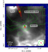 |
Fig. 8 Inner 10 000 au view of the IRAS 18162-2048 high-mass star-forming region. The greyscale image is H2 1-0 S(1) at 2.12 µm. Red contours are VLA X and C bands in the A configuration. Contours are (3, 5, 10, 20, 50, 100, 200) × σX+C, where σX+C = 7µJy beam−1. Green contours are ALMA ∼3.3 mm. Contours are (3, 5, 10, 15) × σ3.3mm, where σ3.3mm = 18µJy beam−1. Black crosses correspond to SINFONI positions. The synthesised beams are shown at the bottom-right corner. |
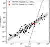 |
Fig. 9 Correlation between bolometric luminosity and radio continuum luminosity at centimetre wavelengths (dashed line and shaded area). Squares represent very low luminosity (Lbol < 1 L⊙), circles low luminosity (1 ≤ Lbol ≤ 1000 L⊙), and triangles high luminosity sources (Lbol > 1000 L⊙). The dot-dashed line represents the expected radio luminosity of an optically thin region photo-ionised by Lyman continuum. The red circle corresponds to a Lbol ∼ 600 L⊙ assuming all radio flux comes from shocked-excited jet emission, whereas the red triangle corresponds to a Lbol ∼ 1300 L⊙ assuming all radio flux comes from an optically thin H II region. Both have been calculated using Sνd2 = 0.55 mJy kpc2, with ν = 8.19 GHz. The figure is adapted from Anglada et al. (2018). |
4.2 Physical conditions of the PDR
There is compelling evidence of the presence of a PDR in IRAS 18162–2048. Our observations indicate that IRS 7/SC is most likely a B2/B3 ZAMS star that has ignited its own compact H II region. The surrounding molecular gas shows clear signatures of UV-pumped H2 emission, confirming the coexistence of ionised, atomic, and molecular phases typical of a PDR.
To investigate the physical conditions governing this region, we used the spectral synthesis and photo-ionisation code Cloudy1. Calculations were carried out with version 25.00 of Cloudy (described by Gunasekera et al. 2025), which includes significant improvements in its treatment of molecular processes and updated atomic and grain physics compared to the widely used versions 13 and 17 (Ferland et al. 2013, 2017).
Following a methodology similar to that of Kaplan et al. (2017), we explored the PDR’s physical properties using a grid of constant-temperature, constant-density models. Although this approach simplifies the geometry, it effectively reproduces the observed H2 ro-vibrational level populations, suggesting that the emitting layer of the PDR can be characterised by relatively uniform conditions. We used the grid command in Cloudy to explore temperatures from 200 to 800 K in steps of 50 K and hydrogen densities from log10(nH /cm−3) = 2.0 to 5.0 in steps of 0.1 dex. The incident radiation field was modelled as a blackbody with an effective temperature of T = 19 000 K, consistent with a B3 V star, and a hydrogen-ionising photon rate of  (Thompson 1984), as obtained from the radio observations. The projected separation between IRS 7/SC and the PDR, derived from our near-IR observations, is 4″ (corresponding to 5600 au, or 0.027 pc), which we specified using the Cloudy command radius 16.92 in units of log10 in centimetres. Standard interstellar medium abundances were adopted, including dust grains and polycyclic aromatic hydrocarbons (PAHs), by enabling the commands grain Orion, grains PAH 3, and database H2. To account for element depletion onto dust, we used the parametrisation of Jenkins (2009) with a depletion strength of F∗ = 0.5. Cosmic background radiation and cosmic ray ionisation were included via the CMB and cosmic ray background options, respectively. The models were run with 3000 computational cells and with the sphere and double keywords to ensure proper convergence for optically thick geometries. A stopping criterion of AV = 20 mag was imposed, motivated by the observed extinction (AV ∼ 12 mag; Sect. 3.3). The calculations were set to iterate until convergence.
A total of 403 models were generated. The goodness of the fit was quantified using χ2 = Σ(ln(Fobs) − ln(Fmodel))2, where Fobs and Fmod are the observed and modelled line flux densities, respectively. Figure 10 (left panel) shows the resulting χ2 contour map. The best-fitting model (χ2 = 1.94) corresponds to T = 600 K and log10(nH /cm−3) = 3.9, i.e. nH = 7.9 × 103 cm−3. The grid strongly constrains the gas temperature, while the density remains poorly constrained, a degeneracy also noted by Kaplan et al. (2017) in their study of the Orion Bar. This behaviour arises because temperature affects the collisional excitation rates and the thermal population of the v = 0 ladder, which in turn determines how higher vibrational levels are populated via UV pumping. As a result, the models are highly sensitive to temperature variations, whereas density exerts a weaker influence. As mentioned in Sect. 3.4, the fitted Tcold component may be a better tracer of the kinetic temperature of the gas, and it is consistent with the temperature of the best Cloudy model.
The right panel of Fig. 10 presents the ro-vibrational excitation diagram for the best-fit model compared with our de-reddened observations, both normalised to the 1–0 S(1) line at 2.12 µm. The agreement is excellent, particularly in reproducing the observed ‘sawtooth’ pattern characteristic of UV-pumped molecular hydrogen. Model-independent estimates of the radiation field strength can be expressed in units of the Habing field (Wolfire et al. 2022) as G0 ∼ 0.5Lbol/(4πl21.6 × 10−3), where Lbol is the stellar luminosity (in erg s−1) and l is the projected distance in cm between the ionising source and the PDR. Using L ∼ 1300 L⊙ ∼ 5×1036 erg s−1 and l ∼ 5880 au ∼ 8.79×1016 cm, we estimated G0 ∼ 1.6 × 10⁴. For comparison, typical field strengths in benchmark PDRs such as the Orion Bar are G0 ∼ 3 × 10⁴ (Wolfire et al. 2022), while Berné et al. (2009) derived values in the range of G0 ∼ 103–105 for Monoceros R2 from the combined analysis of PAH ionisation fractions and H2 0–0 S(3)/S(2) line ratios. The derived parameters, T = 600 K, nH ≈ 8 × 103 cm−3, and G0 ∼ 104, are consistent with those found in other dense PDRs illuminated by early-type stars. The estimated radiation field in IRAS 18162–2048 is therefore consistent with a dense, strongly irradiated PDR powered by a B2/B3 ZAMS star.
Our spectral coverage (1.93–2.47 µm) only includes the near-IR ro-vibrational transitions of H2 and thus misses the pure rotational 0–0 transitions at mid-IR wavelengths (3.3–28.2 µm). These lines, observable only with the James Webb Space Telescope (JWST), would probe the colder gas component of the PDR and provide critical constraints on the gas density and heating balance. Therefore, follow-up JWST observations are warranted to fully characterise the physical structure and excitation conditions in the region IRAS 18162–2048.
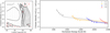 |
Fig. 10 Left: χ2 map for the grid run of constant density and constant temperature with Cloudy. The red star represents the model with the lowest χ2 of 1.94 (see text). The red crosses mark the grid values where the Cloudy code raised a failure flag of failed assert or cloudy abort. Right: Ro-vibrational diagram of H2 comparing our observations (markers) with the best Cloudy model (lines) for T = 600 K and log10(nH /cm−3) = 3.9. Both models and observations have been normalised to the column density over the statistical weight of the 1–0 S(1) line at 2.12 µm (i.e. Nr/gr). Markers and lines are colour-coded by vibrational level (v), and circles and solid lines represent ortho- transitions, whereas triangles and dashed lines are for para-transitions. |
4.3 Multi-generational star formation in IRAS 18162-2048
The high-mass star-forming region IRAS 18162-2048 presents convincing evidence of multi-generational star formation, with young protostars, compact H II regions, and evolved feedback-driven structures coexisting within the same molecular environment. In addition to the well-studied collimated jet driven by the main protostar IRAS 18162-2048, several bubble-like cavities have now been identified across the region (see the H2 continuum subtracted image shown in Fig. 16 from Bally & Reipurth 2023 and Fig. 2 from Mohan et al. 2023). These include bubble-like structures centred on IRS 4, IRS 3, and a third source southeast of MHO 2360 as well as the bubble revealed in this study around IRS 7/SC (see Fig. 1). Such a morphology is more consistent with the cumulative action of multiple photo-ionising sources over time than with purely shock-excited bow shocks from protostellar outflows. However, we cannot rule out that some of this molecular emission emerges from outflow shocked material.
Our VLA detections provide further support for a more evolved stellar population embedded within the region. Both IRS 4 and IRS 3 are clearly detected at centimetre wavelengths, suggesting the presence of ionised gas. Although the lack of equivalent ALMA or near-IR integral field unit coverage prevents a full characterisation of these sources, the spatial coincidence between radio peaks and bubble H2 structures strongly hints at past or ongoing H II regions. We also calculated the number of Lyman continuum photons for the two sources as done for IRS 7/SC (see Sect. 4.1). We obtained  for IRS 4 and
  for the source in the proximity of IRS 3 (see Table 2), both consistent with B2/B3 ZAMS stars. In fact, these sources may represent an older generation of stars, as they are clearly detected in the Hα image of Bally & Reipurth (2023, see their Fig. 1) and therefore had time to disperse their surroundings and lower the extinction. This structure should be considered in conjunction with the newly detected PDR around IRS 7/SC, which our combined near-IR and radio diagnostics favour to be a compact photo-ionised nebula. In this case, however, IRS 7/SC may be in a younger evolutionary stage in comparison to the aforementioned sources.
Taken together, the presence of multiple ionised bubbles and compact radio sources indicates that several massive or intermediate-mass stars have already reached the stage of producing photo-ionising feedback. Meanwhile, the main protostar, IRAS 18162-2048, appears to be significantly younger. Estimates for massive protostars undergoing high accretion rates (10−4–10−3 M⊙ yr−1) predict the development of a compact H II region at ages ∼105 yr (Osorio et al. 1999; Cesaroni et al. 2005; Davies et al. 2011; Mottram et al. 2011). Although Añez-López et al. (2020) suggested the presence of an incipient hyper-compact H II region towards the main protostar, observational evidence remains inconclusive. Our results are consistent with IRAS 18162-2048 still being younger than ∼105 yr and not in the ZAMS stage yet, i.e. prior to fully developing a stable photo-ionised region, while other sources in its vicinity have already reached this evolutionary stage.
This age spread opens the possibility that a triggered star formation process operated in the region IRAS 18162-2048. The spatial distribution of the bubbles appears to surround the central region where the main protostar IRAS 18162-2048 resides. Although speculative at this stage, the geometry towards the main protostar IRAS 18161-2048 may be suggestive of compressed gas being funnelled inwards by previous generations of feedback-driven expansion. Such a sequence of older stars carving cavities followed by the collapse of swept-up material forming younger objects has been proposed in other high-mass star-forming regions (e.g. Lee & Chen 2007; Thompson et al. 2012; Liu et al. 2017; Kim et al. 2025). Nevertheless, the current data do not yet allow for a firm conclusion, and dedicated molecular-line kinematics studies and higher-resolution radio and IR spectro-imaging of the outer bubbles will be required to confirm or refute this scenario.
In summary, the high-mass star-forming region IRAS 18162-2048 is emerging as a clustered sequential star-forming environment where feedback from earlier massive stars has shaped the cloud and may have influenced the birth of the next generation, including the main protostar IRAS 18162-2048. The system therefore provides an excellent laboratory to study the interplay between feedback and star formation in a massive protocluster context.
5 Conclusions
We have presented near-IR integral field spectroscopic observations of the high-mass star-forming region IRAS 18162–2048 obtained with VLT/SINFONI and complemented with new VLA X and C band data and ALMA band 3 observations. Our study resolved the inner ∼10 000 au of the system, revealing a complex interplay between massive and intermediate-mass YSOs, ionised and molecular gas, and UV-irradiated material. Through spectral and morphological diagnostics, we identified clear evidence of a compact H II region and a PDR excited by a B2/B3 type ZAMS star, most likely by IRS 7/SC. We summarise our main conclusions in the following:
The SINFONI K band continuum map reveals two main IR sources, IRS 2 and IRS 7, consistent with previous detections by Yamashita et al. (1987); Tamura et al. (1991); Stecklum et al. (1997). The primary source, IRAS 18162-2048, remains undetected up to 2.47 µm, indicating very high extinction towards the main protostar (Fig. 1);
The IR source IRS 7 shows a peculiar Brγ profile with a narrow emission core superimposed on a broad absorption component, and this is consistent with a B2–B3 ZAMS star following the classification scheme from Bik et al. (2005). The lack of He I and C IV lines rules out O spectral types. We interpret the emission component of the Brγ line as evidence of a nascent compact H II region surrounding IRS 7 and the absorption component as its photosphere (Fig. 3);
Strong H2 ro-vibrational emission was detected, exhibiting the characteristic ‘sawtooth’ pattern in the excitation diagram, which is clear evidence of UV radiation typical of PDRs, rather than the shock excitation. The 1–0 S(1)/2– 1 S(1) ratio (≤5.9) further supports this interpretation and is consistent with dense UV-irradiated molecular gas. Pixel-by-pixel H2 1–0 Q(3)/1–0 S(1) ratios yield an average visual extinction of AV ∼ 12 mag across the main bow-shaped H2 structure, consistent with previous estimates. This moderate extinction enables efficient UV penetration, sustaining the observed H2 emission. The radial velocity map reveals bulk velocities of ∼1 km s−1, further evidencing the dominance of UV radiation. See Figs. 4 and 5;
New high-resolution VLA X and C band observations detected the compact source coincident with IRS 7 (also known in the radio as ‘stationary condensation’), with a flux density of 0.283 ± 0.015 mJy (Fig. 6). For the first time, IRS 7/SC is detected in millimetre wavelengths in our ALMA band 3 observations, with a flux density of 0.457 ± 0.310 mJy (Fig. 7). The spectral index between 3–6 cm and 3.3 mm (α = 0.19 ± 0.27) is consistent with free-free emission. The derived Lyman continuum photon rate for the centimetre regime (Fig. 9) corresponds to a B2/B3 ZAMS star, in excellent agreement with the near-IR spectral diagnostics;
Using the 25.00 Cloudy code (Gunasekera et al. 2025), we modelled the H2 ro-vibrational populations assuming a constant density and temperature. The best-fitted model yielded Tgas = 600 K and nH = 7.9 × 103 cm−3, reproducing the observed ‘sawtooth’ excitation pattern (Fig. 10). A model-independent estimate of the UV radiation field gave G0 ∼ 1.6 × 10⁴ in Habing units, which is similar to estimates inferred for benchmark PDRs such as the Orion Bar and Monoceros R2. This supports the interpretation of IRS 7 as a young massive star photo-ionising and photo-dissociating its surroundings;
Large and small scales near-IR and radio observations revealed multiple compact bubbles associated with sources such as IRS 7, IRS 4, IRS 3, and the structure southeast to MHO 2360, indicating previous episodes of massive-star feedback and the presence of H II regions. The morphology and spatial distribution of these bubbles suggest that earlier generations of stars influenced the cloud structure and potentially helped trigger subsequent star-formation events. While further high-resolution observations are required to firmly establish this scenario, IRAS 18162–2048 stands out as an active, multi-generational, feedback-rich star-forming complex.
Acknowledgements
The authors acknowledge fruitful discussions with K.F. Kaplan, M. Pound, and M. Wolfire. The authors thank the anonymous referee for their constructive report. R.F., G.A., J.F.G., M.O., G.B.C., F.P.M., G.A.F. acknowledge support from the grants PID2023-146295NB-I00, and from the Severo Ochoa grant CEX2021-001131-S funded by MCIN/AEI/10.13039/501100011033 and by “European Union NextGenerationEU/PRTR”. G.B-C also acknowledges support from grant PRE2018-086111, funded by MCIN/AEI/ 10.13039/501100011033 and by ‘ESF Investing in your future’. A.F.P.M. acknowledges support from grant PRE2021-100926, funded by MCIN/AEI /10.13039/501100011033 and by ‘ESF Investing in your future’. A.C.G. acknowledges support from PRIN-MUR 2022 20228JPA3A “The path to star and planet formation in the JWST era (PATH)” funded by NextGeneration EU and by INAF-GoG 2022 “NIR-dark Accretion Outbursts in Massive Young stellar objects (NAOMY)” and Large Gran INAF-2024 “Spectral Key features of Young stellar objects: Wind-Accretion LinKs Explored in the infraRed (SKYWALKER). JMMS acknowledges financial support from the Spanish Ministry of Science and Innovation under grant PID2022-136828NB-C41/AEI/10.13039/501100011033/ERDF/EU and through the María de Maeztu award to the ICCUB (CEX2024-001451-M). R.G.M. acknowledges support from DGAPA-UNAM-PAPIIT project IN105225. C.C.-G. acknowledges support from UNAM DGAPA-PAPIIT grant IG101224. G.A.F also gratefully acknowledges the Deutsche Forschungsgemeinschaft (DFG) for funding through SFB 1601 “Habitats of massive stars across cosmic time” (sub-project B1) and from the University of Cologne and its Global Faculty programme. This paper makes use of the following ALMA data: ADS/JAO.ALMA#2012.1.00441.S. ALMA is a partnership of ESO (representing its member states), NSF (USA) and NINS (Japan), together with NRC (Canada), NSC and ASIAA (Taiwan), and KASI (Republic of Korea), in cooperation with the Republic of Chile. The Joint ALMA Observatory is operated by ESO, AUI/NRAO and NAOJ. This study is also based on observations made under project 19A-321 with the VLA of NRAO. The National Radio Astronomy Observatory is a facility of the National Science Foundation operated under cooperative agreement by Associated Universities, Inc.
References
- Añez-López, N., Osorio, M., Busquet, G., et al. 2020, ApJ, 888, 41 [CrossRef] [Google Scholar]
- Alcalá, J. M., Natta, A., Manara, C. F., et al. 2014, A&A, 561, A2 [NASA ADS] [CrossRef] [EDP Sciences] [Google Scholar]
- Andrews, S. M., Huang, J., Pérez, L. M., et al. 2018, ApJ, 869, L41 [NASA ADS] [CrossRef] [Google Scholar]
- Anglada, G., Villuendas, E., Estalella, R., et al. 1998, AJ, 116, 2953 [Google Scholar]
- Anglada, G., Rodríguez, L. F., & Carrasco-González, C. 2018, A&A Rev., 26, 3 [Google Scholar]
- Aspin, C. 1994, A&A, 281, L29 [NASA ADS] [Google Scholar]
- Bally, J. 2016, ARA&A, 54, 491 [Google Scholar]
- Bally, J., & Reipurth, B. 2023, ApJ, 958, 99 [NASA ADS] [CrossRef] [Google Scholar]
- Beltrán, M. T., & de Wit, W. J. 2016, A&A Rev., 24, 6 [Google Scholar]
- Berné, O., Fuente, A., Goicoechea, J. R., et al. 2009, ApJ, 706, L160 [CrossRef] [Google Scholar]
- Beuther, H., Churchwell, E. B., McKee, C. F., & Tan, J. C. 2007, Protostars and Planets V, 165 [Google Scholar]
- Beuther, H., Kuiper, R., & Tafalla, M. 2025, ARA&A, 63, 1 [Google Scholar]
- Bik, A., Kaper, L., Hanson, M. M., & Smits, M. 2005, A&A, 440, 121 [NASA ADS] [CrossRef] [EDP Sciences] [Google Scholar]
- Burton, M. G. 1992, Austr. J. Phys., 45, 463 [Google Scholar]
- Burton, M. G., Hollenbach, D. J., & Tielens, A. G. G. M. 1990, ApJ, 365, 620 [NASA ADS] [CrossRef] [Google Scholar]
- Busquet, G., Girart, J. M., Estalella, R., et al. 2019, A&A, 623, L8 [NASA ADS] [CrossRef] [EDP Sciences] [Google Scholar]
- Caratti o Garatti, A., Froebrich, D., Eislöffel, J., Giannini, T., & Nisini, B. 2008, A&A, 485, 137 [NASA ADS] [CrossRef] [EDP Sciences] [Google Scholar]
- Caratti o Garatti, A., Stecklum, B., Linz, H., Garcia Lopez, R., & Sanna, A. 2015, A&A, 573, A82 [NASA ADS] [CrossRef] [EDP Sciences] [Google Scholar]
- Caratti o Garatti, A., Stecklum, B., Weigelt, G., et al. 2016, A&A, 589, L4 [NASA ADS] [CrossRef] [EDP Sciences] [Google Scholar]
- Carrasco-González, C., Rodríguez, L. F., Anglada, G., et al. 2010, Science, 330, 1209 [CrossRef] [Google Scholar]
- Carrasco-González, C., Galván-Madrid, R., Anglada, G., et al. 2012, ApJ, 752, L29 [Google Scholar]
- CASA Team (Bean, B., et al.) 2022, PASP, 134, 114501 [NASA ADS] [CrossRef] [Google Scholar]
- Cesaroni, R., Felli, M., Churchwell, E., & Walmsley, M., eds. 2005, IAU Symposium, 227, Massive Star Birth: A Crossroads of Astrophysics [Google Scholar]
- Coffey, D., Bacciotti, F., Podio, L., & Nisini, B. 2010, ApJ, 719, 505 [NASA ADS] [CrossRef] [Google Scholar]
- Costa Silva, A. R., Fedriani, R., Tan, J. C., et al. 2022, A&A, 659, A23 [NASA ADS] [CrossRef] [EDP Sciences] [Google Scholar]
- Crowe, S., Fedriani, R., Tan, J. C., et al. 2024, A&A, 682, A2 [NASA ADS] [CrossRef] [EDP Sciences] [Google Scholar]
- Crowe, S., Fedriani, R., Tan, J. C., et al. 2025, ApJ, 983, 19 [Google Scholar]
- Davies, B., Lumsden, S. L., Hoare, M. G., Oudmaijer, R. D., & de Wit, W.-J. 2010, MNRAS, 402, 1504 [Google Scholar]
- Davies, B., Hoare, M. G., Lumsden, S. L., et al. 2011, MNRAS, 416, 972 [Google Scholar]
- Eisenhauer, F., Abuter, R., Bickert, K., et al. 2003, in Proc. SPIE, 4841, Instrument Design and Performance for Optical/Infrared Ground-based Telescopes, eds. M. Iye, & A. F. M. Moorwood, 1548 [CrossRef] [Google Scholar]
- Elmegreen, B. G. 2011, in EAS Publications Series, 51, EAS Publications Series, eds. C. Charbonnel & T. Montmerle (EDP), 45 [NASA ADS] [CrossRef] [EDP Sciences] [Google Scholar]
- Estalella, R., & Anglada, G. 1999, Introducción a la Física del Medio Interestelar, Textos Docents No. 50 (Barcelona, España: Edicions UB), 140 [Google Scholar]
- Fedriani, R., Caratti o Garatti, A., Coffey, D., et al. 2018, A&A, 616, A126 [NASA ADS] [CrossRef] [EDP Sciences] [Google Scholar]
- Fedriani, R., Garatti, A. C. O., Purser, S. J. D., et al. 2019, Nat. Commun., 10, 3630 [NASA ADS] [CrossRef] [Google Scholar]
- Fedriani, R., Caratti o Garatti, A., Koutoulaki, M., et al. 2020, A&A, 633, A128 [NASA ADS] [CrossRef] [EDP Sciences] [Google Scholar]
- Ferland, G. J., Porter, R. L., van Hoof, P. A. M., et al. 2013, Rev. Mexicana Astron. Astrofis., 49, 137 [Google Scholar]
- Ferland, G. J., Chatzikos, M., Guzmán, F., et al. 2017, Rev. Mexicana Astron. Astrofis., 53, 385 [Google Scholar]
- Frank, A., Ray, T. P., Cabrit, S., et al. 2014, Protostars and Planets VI, 451 [Google Scholar]
- Girart, J. M., Estalella, R., Viti, S., Williams, D. A., & Ho, P. T. P. 2001, ApJ, 562, L91 [Google Scholar]
- GRAVITY Collaboration (Garcia Lopez, R., et al.) 2020, Nature, 584, 547 [Google Scholar]
- GRAVITY Collaboration (Garcia Lopez, R., et al.) 2024, A&A, 684, A43 [Google Scholar]
- Gunasekera, C. M., van Hoof, P. A. M., Dehghanian, M., et al. 2025, arXiv e-prints [arXiv:2508.01102] [Google Scholar]
- Gyulbudaghian, A. L., Glushkov, Y. I., & Denisyuk, E. K. 1978, ApJ, 224, L137 [NASA ADS] [CrossRef] [Google Scholar]
- Jenkins, E. B. 2009, ApJ, 700, 1299 [Google Scholar]
- Kaplan, K. F., Dinerstein, H. L., Oh, H., et al. 2017, ApJ, 838, 152 [CrossRef] [Google Scholar]
- Kim, W.-J., Beuther, H., Wyrowski, F., et al. 2025, A&A, 694, A30 [NASA ADS] [CrossRef] [EDP Sciences] [Google Scholar]
- Klein, R. I., Sandford, M. T., II, & Whitaker, R. W. 1980, Space Sci. Rev., 27, 275 [Google Scholar]
- Kurtz, S., Churchwell, E., & Wood, D. O. S. 1994, ApJS, 91, 659 [Google Scholar]
- Le, H. A. N., Pak, S., Kaplan, K., et al. 2017, ApJ, 841, 13 [Google Scholar]
- Lee, H.-T., & Chen, W. P. 2007, ApJ, 657, 884 [CrossRef] [Google Scholar]
- Liu, T., Lacy, J., Li, P. S., et al. 2017, ApJ, 849, 25 [Google Scholar]
- Marconi, A., Testi, L., Natta, A., & Walmsley, C. M. 1998, A&A, 330, 696 [NASA ADS] [Google Scholar]
- Marti, J., Rodriguez, L. F., & Reipurth, B. 1993, ApJ, 416, 208 [Google Scholar]
- Marti, J., Rodriguez, L. F., & Reipurth, B. 1995, ApJ, 449, 184 [NASA ADS] [CrossRef] [Google Scholar]
- Masqué, J. M., Girart, J. M., Estalella, R., Rodríguez, L. F., & Beltrán, M. T. 2012, ApJ, 758, L10 [Google Scholar]
- Mohan, S., Vig, S., Varricatt, W. P., & Tej, A. 2023, ApJ, 942, 76 [NASA ADS] [CrossRef] [Google Scholar]
- Mottram, J. C., Hoare, M. G., Davies, B., et al. 2011, ApJ, 730, L33 [Google Scholar]
- Najarro, F., Hillier, D. J., & Stahl, O. 1997, A&A, 326, 1117 [NASA ADS] [Google Scholar]
- Nisini, B. 2008, in Jets from Young Stars II, Lecture Notes in Physics, 742, eds. F. Bacciotti, L. Testi, & E. Whelan (Springer-Verlag Berlin Heidelberg), 79 [Google Scholar]
- Osorio, M., Lizano, S., & D’Alessio, P. 1999, ApJ, 525, 808 [Google Scholar]
- Osorio, M., Díaz-Rodríguez, A. K., Anglada, G., et al. 2017, ApJ, 840, 36 [Google Scholar]
- Palla, F., & Stahler, S. W. 1993, ApJ, 418, 414 [Google Scholar]
- Pound, M. W., & Wolfire, M. G. 2023, AJ, 165, 25 [NASA ADS] [CrossRef] [Google Scholar]
- Purser, S. J. D., Lumsden, S. L., Hoare, M. G., et al. 2016, MNRAS, 460, 1039 [NASA ADS] [CrossRef] [Google Scholar]
- Rau, U., & Cornwell, T. J. 2011, A&A, 532, A71 [NASA ADS] [CrossRef] [EDP Sciences] [Google Scholar]
- Ray, T. P., & Ferreira, J. 2021, New A Rev., 93, 101615 [NASA ADS] [CrossRef] [Google Scholar]
- Ray, T. P., McCaughrean, M. J., Caratti o Garatti, A., et al. 2023, Nature, 622, 48 [NASA ADS] [CrossRef] [Google Scholar]
- Rieke, G. H., & Lebofsky, M. J. 1985, ApJ, 288, 618 [Google Scholar]
- Rodriguez, L. F., Moran, J. M., Ho, P. T. P., & Gottlieb, E. W. 1980, ApJ, 235, 845 [Google Scholar]
- Rodríguez-Kamenetzky, A., Carrasco-González, C., Araudo, A., et al. 2017, ApJ, 851, 16 [Google Scholar]
- Sanna, A., Moscadelli, L., Goddi, C., Krishnan, V., & Massi, F. 2018, A&A, 619, A107 [NASA ADS] [CrossRef] [EDP Sciences] [Google Scholar]
- Skrutskie, M. F., Cutri, R. M., Stiening, R., et al. 2006, AJ, 131, 1163 [NASA ADS] [CrossRef] [Google Scholar]
- Stecklum, B., Feldt, M., Richichi, A., Calamai, G., & Lagage, O. 1997, ApJ, 479, 339 [Google Scholar]
- Sternberg, A., & Neufeld, D. A. 1999, ApJ, 516, 371 [NASA ADS] [CrossRef] [Google Scholar]
- Sugitani, K., Fukui, Y., Mizuni, A., & Ohashi, N. 1989, ApJ, 342, L87 [NASA ADS] [CrossRef] [Google Scholar]
- Tamura, M., Gatley, I., Joyce, R. R., et al. 1991, ApJ, 378, 611 [NASA ADS] [CrossRef] [Google Scholar]
- Tan, J. C., Beltrán, M. T., Caselli, P., et al. 2014, Protostars and Planets VI, 149 [Google Scholar]
- Teague, R., & Foreman-Mackey, D. 2018, RNAAS, 2, 173 [NASA ADS] [Google Scholar]
- Thompson, R. I. 1984, ApJ, 283, 165 [NASA ADS] [CrossRef] [Google Scholar]
- Thompson, M. A., Urquhart, J. S., Moore, T. J. T., & Morgan, L. K. 2012, MNRAS, 421, 408 [NASA ADS] [Google Scholar]
- Varricatt, W. P., Davis, C. J., Ramsay, S., & Todd, S. P. 2010, MNRAS, 404, 661 [NASA ADS] [CrossRef] [Google Scholar]
- Wolfire, M. G., Vallini, L., & Chevance, M. 2022, ARA&A, 60, 247 [Google Scholar]
- Yamashita, T., Sato, S., Nagata, T., et al. 1987, A&A, 177, 258 [NASA ADS] [Google Scholar]
- Zannese, M., Guillard, P., Abergel, A., et al. 2025, A&A, 704, A202 [NASA ADS] [CrossRef] [EDP Sciences] [Google Scholar]
- Zapata, L. A., Palau, A., Ho, P. T. P., et al. 2008, A&A, 479, L25 [NASA ADS] [CrossRef] [EDP Sciences] [Google Scholar]
All Tables
VLA X and C band detections in the region IRAS 18162-2048, excluding the main protostar and its jet.
All Figures
|
Fig. 1 Left: SINFONI K band continuum view of the IRAS 18162-2048 star-forming region. The black and white boxes represent the extraction regions for the spectra shown in Fig. 2. The black crosses represent the positions of IRS 2 and IRS 7 (peak intensity pixel from SINFONI), and the red cross shows the position of IRAS 18162-2048 (from the VLA data). Middle left: peak intensity continuum-subtracted map for the Brγ emission line. The white crosses represent the positions of IRS 2 and IRS 7, and the red cross indicates the position of IRAS 18162-2048. Middle right: peak intensity map for the 1–0 S(1) H2 emission line including the continuum emission. Right: same as middle-right panel but with the continuum subtracted. In all panels, the full FoV of SINFONI is shown. |
| In the text | |
|
Fig. 2 Top: spectra for IRS 2 and IRS 7 as labelled. Bottom: spectrum extracted at the highest S/N in the main region of H2 emission. Extraction boxes are shown in Fig. 1. Main H2 emission lines are marked as vertical dashed green lines, Brγ as a dotted green line, and noisy peaks as dotted red lines and labelled as ‘+’. |
| In the text | |
|
Fig. 3 Zoom-in of the IRS 7 spectrum at the 2.07–2.20 µm range. A double Gaussian profile (emission plus absorption) fit to the Brγ line is shown as a dashed red line, whereas the dotted blue line shows the single Gaussian profile fit to the absorption component. Strong emission lines correspond to H2, in particular 2–1 S(3), 1–0 S(1), 3–2 S(4), and 2–1 S(2), at 2.074, 2.122, 2.128, and 2.154 µm, respectively. |
| In the text | |
|
Fig. 4 Left: extinction map obtained from the H2 1–0 Q(3)/1–0 S(1) line ratio. Middle: excitation map from the H2 line ratio 1–0 S(1)/2–1 S(1). Right: radial velocity map using the H2 1–0 S(1) line. In all panels, grey indicates masked pixels with S/N < 3. |
| In the text | |
|
Fig. 5 Ro-vibrational diagram using the fluxes extracted from the white south box depicted in Fig. 1 and summarised in Table 1. The blue circles represent the observed H2 data after extinction correction (AV = 12 mag), and the pink line shows the two-temperature component. The plot was generated using the PDR Toolbox (Pound & Wolfire 2023). |
| In the text | |
|
Fig. 6 Top: VLA X and C band continuum image. The cyan box represents the field shown in Fig. 7, whereas the white box represents the FoV of SINFONI. The main sources in the region are labelled. Middle: same as above but zoomed in on the SINFONI FoV. Contours are (−3, 3, 5, 10, 15) × σX+C where σX+C = 7µJy beam−1. The red crosses represent the VLA positions for IRAS 18162-2048 and IRS 7/SC, and the white crosses are the SINFONI positions for IRS 2 and IRS 7/S. Bottom: zoomed in views of the red boxes in the top panel highlighting IRS 3 (left) and IRS 4 (right). The synthesised beams are shown at the bottom-right corners. |
| In the text | |
|
Fig. 7 Top: ALMA band 3 (∼3.3 mm) image in the region IRAS 18162-2048. Red crosses are ALMA 1.14 mm detections in the field (Busquet et al. 2019), with the larger cross corresponding to the main protostar IRAS 18162-2048. The large white crosses indicate the positions of IRS 2 and IRS 7/SC from their SINFONI positions. The white box represents the SINFONI FoV. Bottom: same as above but zoomed in on the SINFONI FoV. Contours are (−3, 3, 5, 10, 15) × σ3.3mm, where σ3.3mm = 18 µJy beam−1. The synthesised beams are shown at the bottom right corners. |
| In the text | |
|
Fig. 8 Inner 10 000 au view of the IRAS 18162-2048 high-mass star-forming region. The greyscale image is H2 1-0 S(1) at 2.12 µm. Red contours are VLA X and C bands in the A configuration. Contours are (3, 5, 10, 20, 50, 100, 200) × σX+C, where σX+C = 7µJy beam−1. Green contours are ALMA ∼3.3 mm. Contours are (3, 5, 10, 15) × σ3.3mm, where σ3.3mm = 18µJy beam−1. Black crosses correspond to SINFONI positions. The synthesised beams are shown at the bottom-right corner. |
| In the text | |
|
Fig. 9 Correlation between bolometric luminosity and radio continuum luminosity at centimetre wavelengths (dashed line and shaded area). Squares represent very low luminosity (Lbol < 1 L⊙), circles low luminosity (1 ≤ Lbol ≤ 1000 L⊙), and triangles high luminosity sources (Lbol > 1000 L⊙). The dot-dashed line represents the expected radio luminosity of an optically thin region photo-ionised by Lyman continuum. The red circle corresponds to a Lbol ∼ 600 L⊙ assuming all radio flux comes from shocked-excited jet emission, whereas the red triangle corresponds to a Lbol ∼ 1300 L⊙ assuming all radio flux comes from an optically thin H II region. Both have been calculated using Sνd2 = 0.55 mJy kpc2, with ν = 8.19 GHz. The figure is adapted from Anglada et al. (2018). |
| In the text | |
|
Fig. 10 Left: χ2 map for the grid run of constant density and constant temperature with Cloudy. The red star represents the model with the lowest χ2 of 1.94 (see text). The red crosses mark the grid values where the Cloudy code raised a failure flag of failed assert or cloudy abort. Right: Ro-vibrational diagram of H2 comparing our observations (markers) with the best Cloudy model (lines) for T = 600 K and log10(nH /cm−3) = 3.9. Both models and observations have been normalised to the column density over the statistical weight of the 1–0 S(1) line at 2.12 µm (i.e. Nr/gr). Markers and lines are colour-coded by vibrational level (v), and circles and solid lines represent ortho- transitions, whereas triangles and dashed lines are for para-transitions. |
| In the text | |
Current usage metrics show cumulative count of Article Views (full-text article views including HTML views, PDF and ePub downloads, according to the available data) and Abstracts Views on Vision4Press platform.
Data correspond to usage on the plateform after 2015. The current usage metrics is available 48-96 hours after online publication and is updated daily on week days.
Initial download of the metrics may take a while.