| Issue |
A&A
Volume 708, April 2026
|
|
|---|---|---|
| Article Number | A5 | |
| Number of page(s) | 17 | |
| Section | Astrophysical processes | |
| DOI | https://doi.org/10.1051/0004-6361/202558674 | |
| Published online | 25 March 2026 | |
Unveiling broad line region structure in active galactic nuclei with high resolution X-ray spectra
An analytic approach to wind emission line profiles
1
IFPU – Institute for Fundamental Physics of the Universe, Via Beirut 2, 34151 Trieste, Italy
2
SISSA – International School for Advanced Studies, Via Bonomea 265, 34136 Trieste, Italy
3
INAF – Osservatorio Astronomico di Trieste, Via G. B. Tiepolo 11, I-34143 Trieste, Italy
4
Centre for Extragalactic Astronomy, Department of Physics, Durham University, South Road, Durham DH1 3LE, UK
5
Quasar Science Resources SL for ESA, European Space Astronomy Centre (ESAC), Science Operations Department, 28692 Villanueva de la Cañada, Madrid, Spain
6
Astronomical Institute, Tohoku University, 6-3 Aramakiazaaoba, Aoba-ku, Sendai, Miyagi 980-8578, Japan
★ Corresponding author: This email address is being protected from spambots. You need JavaScript enabled to view it.
Received:
19
December
2025
Accepted:
14
February
2026
Abstract
XRISM has provided an unprecedented view of the emission and absorption lines in the X-ray. Notably, early results showed significant complexity to the Fe-Kα line profile in active galactic nuclei (AGN), with clear contributions from at least three emitting structures: an inner disc, intermediary broad line region (BLR) scale material, and an outer torus. This poses a new challenge for the modelling of the emission lines as, while fast sophisticated models for disc line-profiles exist, large scale-height material is typically much more complex. In this paper we aim to address this gap, by building a fully analytic model for the emission line profiles from a wind, aimed towards BLR scale material, motivated on previous reverberation studies suggesting a wind on the inner edge of the BLR. Our approach gives a physically motivated, yet computationally fast, model for the intermediary component to the Fe-Kα complex seen in the XRISM data. We demonstrate our model on the XRISM observations of NGC 4151 from the performance verification phase, showing that it gives a good description of the data, with physically reasonable parameters for BLR scale material. We also show that our model naturally gives the ‘smooth’ line profile seen in the data, due to the large spatial extent of a wind. Finally, we make our model code public to the community, and name it XWIND.
Key words: accretion, accretion disks / line: profiles / X-rays: galaxies
© The Authors 2026
 Open Access article, published by EDP Sciences, under the terms of the Creative Commons Attribution License (https://creativecommons.org/licenses/by/4.0), which permits unrestricted use, distribution, and reproduction in any medium, provided the original work is properly cited.
This article is published in open access under the Subscribe to Open model. This email address is being protected from spambots. You need JavaScript enabled to view it. to support open access publication.
1. Introduction
Accreting systems, typically understood in the context of the Shakura & Sunyaev (1973) disc model, display near-ubiquitous out-flowing winds. From accreting white dwarfs, to black hole binaries, and up to active galactic nuclei (AGN), outflowing material seems to be a direct consequence of accretion, either driven via magnetic fields (e.g. Blandford & Payne 1982; Fukumura et al. 2010, 2017), thermally through inverse Compton scattering (e.g Begelman et al. 1983; Begelman & McKee 1983), or radiatively via the absorption of an incident photon field (e.g. Proga et al. 2000; Proga & Kallman 2004; King 2010).
In AGN the picture is rather complex. In the X-ray there are ultra-fast outflows (UFOs), winds reaching a significant fraction of the speed of light (∼0.2 − 0.3c) typically associated with highly accreting AGN (e.g. Reeves et al. 2009; Tombesi et al. 2010; Nardini et al. 2015; Matzeu et al. 2017; Igo et al. 2020; Xrism Collaboration 2025; Noda et al. 2025b). In the optical ultraviolet, powerful outflows can manifest in both characteristic broad-absorption lines (e.g. Weymann et al. 1991; Leighly et al. 2009, 2018; Choi et al. 2020, 2022) or skewed and blueshifted emission lines. Importantly for our understanding of AGN feedback, these powerful outflows are detected across cosmic time (e.g. Maiolino et al. 2012; Bischetti et al. 2017, 2019, 2023; Fiore et al. 2017), with a clear link between the outflow power and the accretion power in the AGN (e.g. Feruglio et al. 2015; Fiore et al. 2017).
However, the majority of AGN, especially in the local Universe, are not accreting close to the Eddington limit, and so one does not necessarily expect to see these powerful outflows. Yet, even in more typical moderately accreting AGN, there is evidence for winds, albeit with significantly less power than the more extreme UFOs. The clearest examples come from intensive monitoring campaigns, in particular STORM campaigns (De Rosa et al. 2015), which showed clear evidence of variable absorption, now interpreted as a disc wind on the inner edge of the broad line region (BLR) (Dehghanian et al. 2019a,b; Kara et al. 2021). More recently, BLR scale outflows have also been suggested in spatially resolved Gravity and Gravity+ observations (e.g. GRAVITY Collaboration 2024, 2026). Given the prevalence of more moderately accreting AGN and the near-ubiquitous presence of the BLR, understanding the structure of these BLR scale outflows and their link to the accretion flow is critical for our overall understanding of the structure and evolution of AGN.
Large scale-height material has the advantage that it subtends a large solid angle as seen from the central source. Given the ubiquity of high energy X-rays in AGN (Elvis et al. 1994; Lusso & Risaliti 2016), this large scale-height material should see, and absorb, a significant number of X-ray photons. A fraction of these will then be re-emitted, predominantly in Fe-Kα and Fe-Kβ (e.g. Murphy & Yaqoob 2009; Tzanavaris et al. 2023), with the motion of the material imprinted onto the observed line shape. Indeed, previous work using Chandra, XMM, and NuSTAR spectra has clearly shown contributions to the Fe-Kα line from BLR scale material (e.g. Yaqoob & Padmanabhan 2004; Bianchi et al. 2008; Miller et al. 2018; Andonie et al. 2022b,a). This is further supported by Noda et al. (2023) who showed Fe-Kα lagging the continuum through a changing-state event with timescales corresponding to BLR distances.
More recently, XRISM observations of bright nearby AGN have clearly distinguished multiple components of the Fe-Kα complex, consistently showing an intermediary component consistent with BLR scale material (Xrism Collaboration 2024; Bogensberger et al. 2025; Miller et al. 2025; Mehdipour et al. 2025; Kammoun et al. 2025). This provides an opportunity, as resolving individual components of the emission lines allows for the detailed modelling of each of these emitting components. However, herein lies the challenge, as detailed modelling of wind emission lines is generally complex. Firstly, physically realistic modelling of the wind structures requires expensive hydrodynamical simulations (e.g. Proga et al. 2000; Nomura et al. 2016; Nomura & Ohsuga 2017; Higginbottom et al. 2018). This can be circumvented to some extent by implementing parametric models for the wind structure (e.g. Knigge et al. 1995; Sim et al. 2008; Hagino et al. 2015; Matzeu et al. 2022; Luminari et al. 2018, 2024), which allow for rapid calculations of both the velocity and density profiles. This approach is used in a number of current AGN wind models (e.g. the WINE model of Luminari et al. 2024 and the XRADE model from Matzeu et al. 2022, among others). However, in order to extract observable spectra, radiative transfer calculations are required, regardless of whether the wind structure is calculated via simulation or parametrically. Radiative transfer calculations are typically complex, leading to computational bottlenecks, although we note that a number of sophisticated methods currently exist (e.g. Long & Knigge 2002; Odaka et al. 2011; Mehdipour et al. 2016; Ferland et al. 2017; Vander Meulen et al. 2023; Luminari et al. 2023; Matthews et al. 2025). Often, to speed up the fitting process, studies will then resort to calculating model grids to create interpolation tables (e.g. Luminari et al. 2024), or, for more advanced usage, train a convolutional neural net (Matzeu et al. 2022) (emulation). These are highly advanced models, with the ability to fit a full broad-band X-ray spectrum. However, for a slow wind on the inner edge of the BLR, the main constraining power in the X-ray should originate in the Fe-Kα complex, and so full radiative transfer is likely unnecessary.
Instead, it should be possible to perform a simplified analytic calculation. This is the main aim of this paper. Here we parameterise the wind in terms of its geometry, velocity profile, and mass-outflow rate. Through mass-conservation, we then calculate the density profile. Under the assumption that the material is mostly neutral and illuminated by a simple power-law X-ray spectrum, we perform a simplified calculation of the absorption and transmittance of the incident X-ray spectrum through the wind. This approach is analytic and allows us to extract the number of photons re-emitted in Fe-Kα, in essence the emissivity profile. Accounting for the relativistic Doppler shift induced by the wind motion and integrating over the emissivity profile, then gives the observed frame emission line profile. Not only does this provide a rapid calculation of the emission line profile, but it also self-consistently calculates the equivalent width of the line. These combine to give constraining power on not only the distance from the black hole of the wind, but also the mass-outflow rate and covering fraction.
This paper is organised as follows. In Section 2 we define the model and give a detailed description of the calculations. Then in Section 3 we explore the properties of the model and its observables. In Section 4 we apply our model to an XRISM observation of NGC 4151, demonstrating its ability to constrain the properties of a BLR-like wind, before we give our discussion and conclusions in Section 5.
2. XWIND model definition
We give here a detailed overview of the calculations that go into our wind line model. Throughout we will use the standard notation for radii, where r is a dimensionless gravitational radius and R is in physical units, related via R = rRG where RG = GM/c2. The same notation also applies to any other distance measure throughout this paper.
2.1. Wind geometry
We start by defining the geometry of our wind, sketched in Fig. 1, expanding on that initially defined in Sim et al. (2008). Throughout we will work in spherical polar coordinates. For simplicity, we assume the wind is axisymmetric in azimuth, eliminating any dependence on ϕ in the reference frame of the wind.
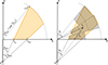 |
Fig. 1. Left: definition of our model geometry. The wind is launched between rin and rout, at an angle defined by the distance of the focus below the origin, df. The covering fraction fcov defines the maximum radial extent of the wind rmax (in spherical polar coordinates), giving a spherical boundary condition. Right: example of our calculation grid (at significantly lower resolution for clarity). We split the wind into cells of cos(θ) with width dcos(θ) in the range cos(θ)∈[0, fcov], and radius r with width dlog(r). The grid in r extends from the inner streamline to either the outer streamline (defined from rout) or rmax, depending on whichever is smallest. Our wind cells are illustrated as the dark shaded regions. Throughout this paper we will evaluate the wind emission and density at the centre of each cell θi and rj. For completeness, this also defines the length travelled along the streamline lij at each cell. |
As in Sim et al. (2008) the wind is launched between rin and rout. We consider the wind to consist of a set of streamlines, each with an opening angle αij, which all converge at a focal point df located on the z-axis directly below the origin. We treat this focal point as an input parameter throughout our calculations. The maximum extent of the wind is then set by the covering fraction fcov, defined in terms of the total solid angle fcov = Ω/4π. While this assumes that the wind is launched from both sides of the disc, the observer will only see emission originating from the side of the disc facing the observer. This gives a spherical boundary condition of rmax defined as
 (1)
(1)
where cos(θmin) = fcov (from the definition of the solid angle). We stress that this boundary condition is only valid if arccos(fcov) > arctan(rin/df), as otherwise the opening angle of the wind is too shallow to ever reach the desired covering fraction. In these instances, our model code sends a warning, and then readjusts fcov, before proceeding with the calculation.
We now depart somewhat from the geometry in Sim et al. (2008), here opting to divide our wind into cells in θ and r. We define bins in cos(θ), spaced at a constant dcos(θ) = 0.002, in the range cos(θ)∈[0, fcov]. This naturally leads to each wind cell subtending the same solid angle dΩ = dϕdcos(θ) as seen from the central source. When evaluating wind properties, we use the centre of each bin, defined as θi = cos(θedge)+0.5dcos(θ), where θedge is the lower edge of the bin.
For each θi, we then subdivide into bins of r, geometrically spaced such that dlog(r) = 0.01 is constant. Here, the radial bin edges are defined from the point where the sight-line along θi crosses the streamline launched from rin to the point where the sight-line either crosses the streamline from rout or crosses rmax, whichever is the smallest. As with θ, we evaluate the wind properties in the centre of the bin, defined as rj = redge + 0.5 × 10log10(redge)+dlog(r).
The wind is now tiled with a set of cells, each with evaluation points θi and rj. This is illustrated on the right side of Fig. 1. Each of these cells corresponds to a streamline launched at rL, ij with opening angle αij, and evaluated at a length lij along the streamline. All of these are given by
![Mathematical equation: $$ \begin{aligned} \cos (\alpha _{ij})&= \frac{r_j \cos (\theta _i) + d_f}{\big [r_j^2 + 2r_j d_f \cos (\theta _i) + d_f^2\big ]^{1/2}}, \end{aligned} $$](/articles/aa/full_html/2026/04/aa58674-25/aa58674-25-eq2.gif) (2)
(2)
 (3)
(3)
![Mathematical equation: $$ \begin{aligned} l_{ij}&= \big [r_j^2 + r_{L, ij}^2 - 2r_j r_{L, ij} \sin (\theta _i)\big ]^{1/2}. \end{aligned} $$](/articles/aa/full_html/2026/04/aa58674-25/aa58674-25-eq4.gif) (4)
(4)
2.2. Velocity profile
The velocity profile can now be easily calculated for each wind cell. Starting with the azimuthal velocity vϕ, we assume that at the base of the wind the streamline has the same azimuthal velocity as the disc, here taken to be Keplerian. As material travels out along the streamline, angular momentum is conserved, such that the azimuthal velocity at any point in the wind is (Knigge et al. 1995)
 (5)
(5)
Note that here we have removed the explicit reference to the cell indexes i and j.
The second component is the outflow velocity along a streamline. Here we use the velocity profile parameterised in terms of the velocity at infinity v∞ (Knigge et al. 1995; Sim et al. 2008; Hagino et al. 2015, 2016; Matzeu et al. 2022)
 (6)
(6)
Here, v0 is the initial velocity at the base, which we fix to 0 throughout, rv is the velocity scale-length, defined as the distance along the streamline where the velocity reaches half of v∞, β is the velocity exponent that determines the acceleration rate along a streamline, and l is the distance along the streamline, previously given in Eq. (4).
2.3. Density profile
Given the defined geometry and the corresponding velocity profile, we can now estimate the density profile of the wind, following Matzeu et al. (2022). We start by considering the total mass-outflow rate Ṁw. It is often easier to express this in terms of the Eddington mass-accretion rate ṀEdd, as this naturally scales by the mass of the central object such that ṁw=Ṁw/ṀEdd.
The mass outflow is distributed between rin and rout, with a mass-loss rate per unit area given by  . Here, κ determines the efficiency of the wind as a function of the physical launch radius. For radiatively driven outflows, the expectation is that κ ∼ −1.3 → −1 (Behar 2009), which effectively states that the majority of material is launched from the inner edge of the wind, with the outflow becoming increasingly inefficient as the launch radius increases.
Mass conservation requires that
 (7)
(7)
This is simply the integral across the surface of the disc covered by the wind (i.e. the annulus between rin and rout), and the factor of 2 comes from the disc having two sides. This can be solved analytically, to give
![Mathematical equation: $$ \begin{aligned} \frac{d\dot{M}_{\rm w}}{dA}&= \frac{\dot{M}_{\rm w} (\kappa + 2)}{4\pi [R_{\mathrm{out}}^{\kappa + 2} - R_{\mathrm{in}}^{\kappa +2}]} R_L^{\kappa } \nonumber \\&= \frac{\dot{m}_{\rm w} \dot{M}_{\mathrm{Edd}} (\kappa + 2)}{4\pi [r_{\mathrm{out}}^{\kappa +2} - r_{\mathrm{in}}^{\kappa +2}]} r_L^{\kappa } R_G^{-2}. \end{aligned} $$](/articles/aa/full_html/2026/04/aa58674-25/aa58674-25-eq9.gif) (8)
(8)
For a given wind cell, we can write the mass density as ρ = dM/dV, where dV = dAdz. Furthermore, within a cell the material has a velocity along the streamline vl, such that in time dt it has travelled dz = vldt. Hence, we can write dV = vldtdA, such that  . The number density in a wind cell is then given by
 (9)
(9)
where mI ≃ 1.23mp is the ion mas, which we choose to write in terms of the proton mass mp. The left column of Fig. 2 demonstrates the density profile for a wind launched at BLR-like distances over a range of outflow velocities.
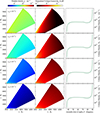 |
Fig. 2. Wind density profile (left column) and corresponding emissivity profile (middle column) for a range of outflow velocities (increasing from top to bottom, value given in top left corner of each row). The right column shows the column-density profile for varying lines of sight through the winds. These have all been calculated for a wind launched between rin = 1000 and rout = 3000, with |

2.4. Calculating the emissivity
An important aspect in the shape of the emission line is the relative emissivity across the wind volume. For a photoionised line, this can be calculated from an incident spectrum and wind density profile. We give here an overview of our methodology for this, based on the neutral Fe-Kα line. We stress that the calculations below give self-consistent solutions to the Fe-Kα line strength; however, for other emission lines this is not the case. Hence, within XWIND, we provide two submodels: XWINDLINE, where the normalisation should remain free for generic use, and XWINDFE, where the normalisation is self-consistently calculated for neutral Fe-Kα and the rest-frame emission assumes the 7-Lorentzian approximation from Hölzer et al. (1997). Internally, the calculations are identical, since XWINDLINE uses the emissivity calculated assuming neutral Fe-Kα. We also use XWINDLINE to extract a convolution kernel, XWINDCONV, allowing for the application of wind broadening to any spectral-shape, including continuum. Throughout we neglect the Compton shoulder in XWIND, as the typical wind densities are too low for this to be important, with the exception perhaps at the base of the wind.
We base our calculations on the analytic approach given in Yaqoob et al. (2001), updated in Tzanavaris et al. (2023). Firstly, the wind will see an incident spectrum, N(E), originating from the central regions of the accretion flow. The relevant part of the spectrum depends somewhat on the line species being calculated, due to strongly differing ionisation potentials. However, this is too complex for our approach. Instead we assume that the relative emissivity across the wind volume is more or less identical for each line species (i.e. that for all lines it traces density), and only the absolute (i.e. normalisation) emissivity differs. Thus, internally we calculate the absolute emissivity for neutral Fe-Kα, and simply apply the same emissivity for any other line.
The neutral Fe-Kα line is induced by photons above EK ≃ 7.1 keV. In this energy range the intrinsic emission is dominated by inverse Compton scattering, giving a power-law-like spectrum (Haardt & Maraschi 1993; Haardt et al. 1994). Hence, we fix the incident spectrum to a power-law of the form N(E) = N0E−Γ, photons s−1 cm−2 keV−1. In XWINDFEN0 is the number of photons s−1 cm−2 at 1 keV. Following Tzanavaris et al. (2023), the Fe-Kα photon flux emitted from a constant column-density material with solid angle Ω is
 (10)
(10)
where y ∼ 0.3 is the fluorescent yield, AFe ≃ 4.86 × 10⁻⁵ (Anders & Grevesse 1989) is the iron abundance, NH is the column-density of the absorbing material, and σFe-K is the iron K-shell absorption cross-section. The cross-section decays exponentially with energy above the absorption edge, such that σFe-K(E) = σ0(E/EK)−α where α ≃ 2.67 and σ0 ≃ 3.37 × 10⁻²⁰ cm2 (Murphy & Yaqoob 2009; Tzanavaris et al. 2023).
Of course, our wind does not have a constant column-density. Instead, this needs to be calculated separately for each wind cell. Making the simplifying assumption that the density within a single wind cell is roughly constant, we can write for the column-density in cell ij: NH, ij ≃ nijΔRj, where ΔRj = rjRGdlog r is the radial width of the wind cell, and is calculated directly from the model geometry.
As we integrate radially along a sight-line θi, not only does the column-density evolve, but also the spectrum incident in the wind cell. For a given cell at (θi, rj), the incident spectrum N(E) will be slightly absorbed by the cell at (θi, rj − 1). Hence, the fluorescence of each cell is not simply calculated directly from Eq. (10). Instead, we need to take into account the effect of all radially preceding cells on the incident spectrum, such that for a wind cell ij in (θi, rj), the incident spectrum is given by
 (11)
(11)
and so the fluorescence from the wind cell at ij is
 (12)
(12)
which now also takes into account the solid angle of each wind cell as seen from the central source. In Eqn. 11, all factors of M cancel (by expanding RG and ṀEdd), such that the total fluorescence and line profile are fully independent of mass.
2.5. Calculating the overall line profile
The previous subsection only gives the emission in the co-moving frame of the wind. In the observer frame, the emission will be smeared out into a characteristic line shape. Material moving away or towards the observer will broaden the line due to Doppler shifts, the bulk outflowing motion of the wind will give a net blueshift, and relativistic length contraction and time-dilation will lead to a boosting effect in the emission originating from material travelling towards the observer. All of these are very well known effects, which have previously been calculated for accretion discs (Chen et al. 1989; Fabian et al. 1989). In this section, we give a generalisation to a 3D velocity profile, though only in the weak field limit.
In general, the energy of the emitted photon is given by the projection of the photon four-momentum, pα, onto the four-velocity of the emitting material, uα, such that Eem = uαpα (Cunningham 1975; Luminet 1979). This will give the usual relation for the special relativistic Doppler shift in a flat space-time, as considered here.
The four-velocity of the emitting material is simply given as uα = gαβuβ = γ(c, −vw) where vw is the three-velocity profile of the wind, γ = (1 − (vw/c)2)−1/2 is the Lorentz factor of the wind material, and gαβ is the Minkowski metric. The three-velocity components of the wind were previously calculated in section 2.2, such that in Cartesian coordinates
 (13)
(13)
The four-momentum of a photon is simply given by  , where
  is a unit vector that describes the direction of the photon. Energy is conserved along a trajectory, and so here Eγ = Eobs (Cunningham 1975). Further, since we assume the photon travels in straight lines, the photon direction is simply
  for an observer located in the x − z plane at an inclination i from the z-axis. Hence, we arrive at the ratio between observed and emitted frame photon energies, considering special relativity only
![Mathematical equation: $$ \begin{aligned} \begin{split} \frac{E_{\mathrm{em}}}{E_{\mathrm{obs}}} = \frac{u_\alpha p^\alpha }{E_{\mathrm{obs}}} =&\gamma \Bigg \{1 - \frac{1}{c} \bigg [v_l\cos (\alpha )\cos (i) \\&+\sin (i) \Big (v_l\sin (\alpha )\cos (\phi ) - v_\phi \sin (\phi ) \Big ) \bigg ] \Bigg \}. \end{split} \end{aligned} $$](/articles/aa/full_html/2026/04/aa58674-25/aa58674-25-eq20.gif) (14)
(14)
As expected, this is in the form of the special relativistic Doppler shift, except that here it is decomposed into individual velocity components. Also, factoring in the gravitational redshift, calculated in the Schwarzchild metric, gives the following
![Mathematical equation: $$ \begin{aligned} \begin{split} \frac{E_{\mathrm{em}}}{E_{\mathrm{obs}}} =&\gamma \bigg (1 - \frac{2}{r} \bigg )^{-\frac{1}{2}}\Bigg \{1 - \frac{1}{c} \bigg [v_l\cos (\alpha )\cos (i) +\\&\sin (i) \Big (v_l\sin (\alpha )\cos (\phi ) - v_\phi \sin (\phi ) \Big ) \bigg ] \Bigg \}. \end{split} \end{aligned} $$](/articles/aa/full_html/2026/04/aa58674-25/aa58674-25-eq21.gif) (15)
(15)
The above only gives the relation between the emitted and observed photon energies. To relate this to an observed photon flux, we take advantage of the fact that Nγ/E3 is Lorentz invariant (Lindquist 1966; Cunningham 1975), such that
 (16)
(16)
where Nγ, em is calculated from Eq. (12).
The total line-profile comes from integrating over the wind volume. However, since we do not know a priori what wind cells correspond to what specific energy shift, it is simpler to iterate over each cell, calculate the photon flux and energy shift from Eqs. (12), (15), and (16), adding the output photon flux to the relevant energy bin.
Throughout we use an internal fractional energy grid in E/E0, with bins evenly spaced from E/E0 = 0.2 to 4.4 with Δ(E/E0) = 2 × 10⁻⁴. This allows for maximum velocity widths up to 0.9c, which is more than adequate for any realistic wind. It also gives an internal energy resolution of 1.2 eV at 6 keV, oversampling that of XRISM-resolve (∼5 eV at 6 keV, Kelley et al. 2025).
As a sanity check, we apply our above methodology to a disc geometry, allowing for a direct comparison to DISKLINE (Fabian et al. 1989). This shows generally very good agreement for large radii, but begins to deviate systematically below r ∼ 50 (see Appendix B, Fig. B.1). This is expected, since DISKLINE considers a treatment using the Schwarzchild metric (though no light-bending). As such, we do not recommend the use of our model code for small launch radii.
3. Model properties
3.1. Emission line profiles
We illustrate the model emission line profiles in Fig. 3. We illustrate the effects by varying each parameter individually while keeping the others fixed. The fixed underlying model is calculated for ṁw= 10−2, rin = 1000, rout = 3rin,  , fcov = 0.6, v∞ = 10−3, rv = 100, β = 1, and κ = −1. All line profiles have been normalised to unity, in order to highlight changes in the shape, and are observed at an inclination of 45 degrees.
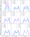 |
Fig. 3. Example emission line profiles and their evolution with varying wind parameters. These have all been re-normalised to have the same total flux, and have all been calculated for an observed inclination of 45 degrees. Each panel shows the effect of varying an individual parameter, given in the top left corner of each panel. When not being varied, parameters are fixed at: ṁw= 10−2, rin = 700, rout = 3rin, |

To start with, there is a clear trend in that the vast majority of the line profiles appear rather sharp. This is not surprising when we examine the emissivity profiles in Fig. 2. In general, the emission is dominated by the inner edge at the base of the wind, as this is where both the density and incident flux is the strongest. At larger distances along the streamline, the density drops off such that the absorption becomes less efficient, resulting in fewer photons available to re-emit. Alternatively, for lines of sight passing through a dense region (e.g. at the base), the optical depth will be high, and so the incident continuum is mostly absorbed before it reaches the outer edge of the wind. This is clear in Fig. 3, which shows almost no change in the line profile when changing rout.
In terms of understanding the physical origin of the wind, the key parameters are rin, v∞, and ṁw. The combination of rin and v∞ should inform the driving mechanism of the wind. Especially radiation-driven outflow models, for example, UV line-driven winds (Proga et al. 2000; Proga & Kallman 2004), FRADO models (Czerny & Hryniewicz 2011; Naddaf et al. 2021), tend to have a specific radial range over which they can exist, as they strongly depend on the local disc SED, as well as contain predictions on the outflow velocity. As both of these have a significant impact on the line profile, it should be possible to constrain them.
The behaviour of the line profile with v∞ also reveals a key effect of calculating the density profile via mass-conservation. As the velocity is reduced, the overall density of the wind increases. In addition, it appears from Fig. 2 that the moderate to high density regions also move further up the streamline. This will then increase the fraction of the emission originating from larger distances along a given streamline within the wind, which in turn traces a smaller angular velocity due to the conservation of angular momentum. The net effect is that the line profile begins to ‘fill in’ towards the centre.
3.2. Fe-Kα equivalent width
A key advantage of our approach is that it gives a self-consistent normalisation to the Fe-Kα emission line for a given wind density profile and incident X-ray spectrum (as also outlined in Tzanavaris et al. 2023). This depends strongly on both the mass-outflow rate ṁw and outflow velocity profile (governed by v∞), as these determine the density profile. We demonstrate this in Fig. 4. This shows on the left the expected equivalent width of the Fe-Kα line for a grid of ṁw and v∞. On the right, we show curves of growth with ṁw and v∞ respectively. These are calculated for the same base model as the line-profiles in Fig. 3. The equivalent widths are calculated with respect to the incident continuum (a power-law, see Section 2.4) at (rest-frame) 6.4 keV.
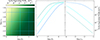 |
Fig. 4. Left: colour-plot showing the equivalent width of the Fe-Kα emission line for varying ṁw and v∞. The darker the shade of green, the larger the equivalent width. The vertical, horizontal solid, and dashed lines correspond to the slices used to extract the curves of growth on the right as a function of ṁw/v∞. Right: curves of growth as a function of ṁw (left panel) and v∞ (right panel). As ṁw increases, so does the equivalent width, until eventually the line saturates due to the wind becoming optically thick. Conversely, increasing v∞ will reduce the equivalent width, as this reduces the overall density of the wind (see Fig. 2) leading to a lower degree of absorption and thus fewer photons available to re-emit as Fe-Kα. |
These behave as expected. Increasing ṁw leads to more material in the wind, and therefore naturally the density increases. Higher density leads to increased absorption of the incident spectrum, which in turn gives a higher number of available photons to re-emit. The perhaps more interesting effect is the saturation of the equivalent width once ṁw reaches a certain value. This is an effect of the wind going optically thick, and so now the limiting factor to the total fluorescence depends on the incident continuum rather than the wind density profile. However, increasing the normalisation of the incident continuum does not lead to a higher equivalent width, as this is always measured relative to the continuum. Hence, we predict a rather stringent upper limit on the expected Fe-Kα equivalent width from a wind of EW ∼ 5 × 10⁻¹ keV (for a covering fraction of 0.6; the exact value will naturally also depend somewhat on fcov). This also becomes clear in Fig. 2, which shows how the emission becomes strongly concentrated to the inner edge of the wind when the density is sufficiently high, such that the incident spectrum is highly absorbed before reaching the inner or outer regions (top panel).
4. Application to XRISM data – a wind on the inner edge of the BLR in NGC 4151?
We demonstrate our model on a XRISM observation of NGC 4151, taken during the performance verification (PV) phase. NGC 4151 was observed five times during the PV phase (Xrism Collaboration 2024; Xiang et al. 2025). We chose the longest observation to maximise signal-to-noise (obsID 300047020, observation date 18.05.2025, exposure time 103.7 ks, presented previously in Xiang et al. 2025).
Before constraining the line-profile, we also fit the broad-band continuum, using simultaneous XRISM-xtend (Noda et al. 2025a) and NuSTAR data. Below we give details on the data reduction, broad-band spectral fit, and finally our fit to the XRISM-resolve (Kelley et al. 2025) spectrum of the Fe-Kα complex.
For all subsequent analysis, we use the reduction pipelines included in HEASOFT v.6.63 and XSPEC v.12.15.1 (Arnaud 1996). All errors are quoted at 90% confidence.
4.1. XRISM-data reduction
We reduce both the XRISM-resolve and XRISM-xtend data, using the standard XRISM reduction pipeline along with the corresponding most recent calibration files from the CALDB database (as of writing, corresponding to the resolve and xtend calibration files from 15 September 2025, and the general files from 15 November 2024). We give here a brief overview of the reduction process, as also outlined in Xrism Collaboration (2024).
We start by running XAPIPELINE, which generates the cleaned event files for both resolve and xtend. Next, focusing on XRISM-resolve, we use XSELECT to extract the source spectrum, filtering such that we only extract high-resolution primary (Hp) events. We also filter out periods of high particle background and data from pixel 27 (as recommended due to a significant variation in gain). Using RSLMKRMF we then generate an RMF file, setting the size option to large (L) to accurately give the response around our region of interest (5–7 keV), but without the significant increase in file size that comes with including the electron loss continuum (the x-large option). For the ancillary response (ARF) file, we first generate an exposure map using XAEXPMAP, before then generating the ARF using XAARFGEN. Here we set the source type to a point-source, and run the ray-tracing of reflected and transmitted photons through the detector using 300 000 photons.
For XRISM-xtend we extract a source spectrum from a rectangular region with dimensions 2.3″ × 5.0″ centred on the source. We then extract a background spectrum using the same extraction region, but on a portion of the sky with no source contribution. The RMF file is generated using XTDRMF and an ARF file in an identical manner to XRISM-resolve (but with the instrument set to xtend).
For both spectra, we bin the data in such a way that each bin contains at least 25 counts, allowing the use of χ2 statistics during the fitting procedure.
4.2. NuSTAR data reduction
Simultaneous with the XRISM observation, NGC 4151 was observed by NuSTAR (obsID 60902010004, presented previously in Xiang et al. 2025). We combine these data with the XRISM-xtend data to extend our broad-band continuum fit to 90.0 keV.
We use the standard NUPIPELINE tool to generate the cleaned event files, with CALBD calibration files corresponding to the most recent update as of writing (released 06 October 2025). After generating the cleaned event files, we run NUPRODUCTS to give both the source and background spectral files, the response file, and the ancillary response file for both FPMA and FPMB modules. The source spectrum is extracted using a circular annulus with a radius of 120″ centred on the source, while the background is extracted from an identical annulus in an empty patch of sky. As with the XRISM spectra, we re-bin the source spectrum to contain at least 25 counts per bin.
4.3. Broad-band spectral fit
Before constraining the profile of the Fe-Kα complex, we require an estimate of the underlying continuum. This is for two reasons. The first is that the intrinsic source continuum flux above ∼7.1 keV determines the absolute strength of the Fe-Kα fluorescence line (see Eq. (10)). The second is that broad features in the line profile are highly sensitive to the shape of the underlying continuum; especially if these features are weak.
Following Noda et al. (in preparation) we construct a phenomenological model for the underlying continuum, using here the combined XRISM-xtend and NuSTAR data. At low energies below ∼1.5 keV the XRISM-xtend spectrum is dominated by a complex scattered continuum. Hence, we limit the XRISM-xtend energy range to 1.2 − 12 keV during the fitting, where we note that part of the scattered continuum is included in order to estimate its contribution to the overall flux level. For NuSTAR, we consider the energy range between 5.0 and 90.0 keV, giving a total combined band-pass of 1.2–90 keV. The total source spectrum is shown in Fig. 5.
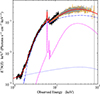 |
Fig. 5. Best fit broad-band continuum, using combined XRISM-xtend (black crosses) and NuSTAR (orange and grey crosses for FPMA and FPMB respectively).The solid red line shows the total spectral model, with the dotted and dashed lines showing the individual components. These are: the scattered continuum (dotted blue), reflection spectrum (dashed magenta), and the primary continuum (dashed-dotted blue). The plotted NuSTAR data have been corrected by a cross-calibration constant used to account for instrumental differences between XRISM-xtend and NuSTAR. The data have been re-binned slightly for clarity. |
In the primary continuum we use a redshifted cutoff power-law (ZCUTOFFPL in XSPEC), subject to absorption from the host galaxy (TBABS Wilms et al. 2000) and also partial covering absorption intrinsic to the AGN itself (e.g. from a wind) (PCFABS). We then include a component originating from cold reflection off the disc (PEXMON Magdziarz & Zdziarski 1995; Nandra et al. 2007) convolved with Gaussian broadening (GSMOOTH) to account for the iron emission and Compton hump. Here we fix the observer inclination at 60 degrees and all abundances to solar abundances. Finally, we include an additional cutoff power-law, with photon index and cutoff energy tied to the primary continuum, to describe the scattered continuum. The total model is then also absorbed by our galaxy, where we fix NH = 2 × 1020 cm−2. The final XSPEC model is then: tbabsMW * (zcutoffplscatt+ tbabsint*(pcfabs*zcutoffplprimary + gsmooth*pexmon)). We also include a cross-calibration constant, applied to the NuSTAR data, to account for small calibration differences between XRISM-xtend and NuSTAR.
This gives a moderate fit to the broad-band spectrum, with χν2 = 4876/3760 = 1.3. The increase in χ2 is predominantly driven by complexity in the scattered continuum and in the region 5 − 8 keV where details in the Fe-Kα profile not captured by this model, as well as absorption lines (as seen in Xiang et al. 2025) not included here, drive significant residuals. As these are a known effect, and since the broad-band continuum shape is otherwise well constrained, we continue with this as our underlying base continuum for our more detailed analysis of the XRISM-resolve spectrum in the next subsection. The best fit continuum model is shown in Fig. 5, with corresponding fit parameters shown in Table 1. The errors are estimated at 90% confidence from an MCMC chain using 8 walkers and 160 000 steps.
Best fit parameters to the broad-band fit of the XRISM-xtend and NuSTAR data.
4.4. Model application to XRISM-resolve
We now focus our analysis onto the XRISM-resolve spectrum. Specifically, we focus on the shape of the Fe-Kα complex and so limit the spectral fit to the energy range 5.0 − 6.6 keV (in the observed frame).
For the underlying continuum we take the model from the broad-band spectral fit, fixing all parameters to those in Table 1. We make one change, removing the RDBLUR*PEXMON component, since we now focus on a detailed fit of the Fe-Kα complex. Xrism Collaboration (2024) showed three distinct components to the Fe-Kα line, which we adapt here. We start with a MYTORUS (Yaqoob 2012) component, convolved with RDBLUR (Fabian et al. 1989), to account for the narrow Torus emission. Specifically, we used the updated MYTORUS line emission files (mytl_V000HLZnEp000_v01.fits) from Yaqoob (2024) as these include the intrinsic Fe-Kα profile from Hölzer et al. (1997). In RDBLUR we fix the emissivity index to −2 to account for the non-disc geometry of the torus, and set a lower limit of 104 RG for the inner radius. We fix the outer radius at 107 RG.
Next we add a XWINDFE component, to account for the moderately broad BLR scale emission, the main focus of this analysis. We stress that XWINDFE will self-consistently calculate the equivalent width of the line for a given input spectrum, and also includes the intrinsic Hölzer et al. (1997) profile for the rest-frame emission (see Section 2 for a full model description). Hence we tie the input spectrum for XWINDFE to that of the primary continuum in the broad-band fit. We also fix a number of the geometric parameters in order to simplify the fit. Firstly, we set the outer launch radius to rout = 1.5rin, since we are aiming to describe a wind on the inner edge of the BLR, so this will in effect limit the radial extent of the wind. Secondly, we fix  , effectively fixing the opening angle on the inner edge to αmin = 30° (see Fig. 1). In the geometry considered here, this also sets an upper limit on the covering fraction of fcov, max ≃ 0.86. From Fig. 3 we see that the velocity parameters rv and β, as well as the radial launch efficiency parameter κ, have only a small impact on the overall line shape. Hence, we fix these at rv = 200, β = 1, and κ = −1, as typically done for radiative winds (e.g Matzeu et al. 2022). During initial fitting attempts, we also noted that the fit was insensitive to turbulent velocity vturb, therefore we fixed this at 0 (where the choice is motivated by the fact that this allows the code to skip an additional convolution step, speeding up the fit). We also fixed all abundances to their solar values, using the values from Anders & Grevesse (1989).
Finally, we include a DISKLINE (Fabian et al. 1989) component, to account for the presence of an inner accretion disc. We allow the inner radius to be free, but fix the outer radius to 103 RG. We also fix the emissivity index to −3, as expected for a flat disc.
Thus, the final XSPEC model is: tbabsMW * (zcutoffplscatt + tbabsint * (pcfabs*zcutoffplprimary + rdblur*mytorus + zashift*(xwindfe + diskline))), where the ZASHIFT component accounts for the lack of a redshift parameter in both XWINDFE and DISKLINE. In Appendix C we test the effect of removing individual model components of the Fe-Kα complex in order to assess their significance for the overall fit.
This gives an excellent fit to the 5.0 − 6.6 keV XRISM-resolve spectrum, with  . The resulting fit parameters are given in Table 2, and the spectrum is shown in Fig 6, where we have elected to only show the 6.0–6.6 keV range in order to highlight the Fe-Kα complex.
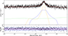 |
Fig. 6. Top: best fit model to XRISM-resolve data (black points). The solid red line shows the total model, while the dashed and dotted lines show the components. These are: scattered and primary continuum (grey dotted lines), MYTORUS emission line from Compton thick slow-moving material (orange dashed line), XWINDFE emission line for a wind inwards of the BLR (blue dashed line), and DISKLINE emission line from the inner disc (green dashed line). Bottom: data-model residuals, normalised by the data errorbar. The shaded blue bands show the 1σ (dark) and 2σ (light) deviation. |
Best fit parameters for the model fit to the Fe-Kα complex in the XRISM-Resolve spectrum.
The resulting XWINDFE parameters suggest a slow-moving wind (log10(v∞/c)≃ − 3.5) with a moderately low mass-outflow rate (log10ṁw ≃ −3.0). Specifically, the mass-outflow rate is important, as this is significantly lower than the accretion rate for NGC 4151 (ṁ ∼ 0.02, Mahmoud & Done 2020), indicating that although the impact on the line-profile is significant, the impact of this slow wind on accretion flow will likely be minimal. In some sense, this is reassuring, given the near ubiquitous presence of a BLR across the AGN population.
However, the inferred outflow velocity, v∞/c ≃ 10−3.5 ≃ 100 km s−1, appears rather low, especially given that the escape velocity at rin ≃ 1550 is vesc ∼ 7600 km s−1. This is likely because our model only considers outflowing material in a wind geometry. More realistic BLR geometries are probably multi-component, with a non-outflowing virialized component and potentially also an inflowing component. Indeed, the physically motivated FRADO models Czerny & Hryniewicz (2011) for the BLR give material that first rises in a dusty wind, before failing and falling back towards the disc. As such, we caution the reader that assuming the entire BLR can be modelled with XWIND, as done here for demonstrative purposes, is likely physically incomplete, and a more realistic picture could be obtained by including some contribution from non-outflowing material. However, this is beyond the scope of this paper; instead, we note that XWIND does give a physically motivated method for adding in a wind component to the BLR emission. Additionally, Kraemer et al. (2006) suggests that this wind component should be present, as seen through slow-moving, ∼500 km s−1, material seen in absorption.
More interesting in terms of the wind itself is the resulting density profile, as seen in Fig. 7. Initially, one would think that the low outflow rate would give a relatively low density. However, this is counteracted by the low outflow velocity, instead giving a moderate density range of ∼107 − 109 cm−3. Although the high density regions are concentrated towards the base of the wind, the larger scale regions appear to have a relatively uniform profile, with n ∼ 107.2 − 107.5 cm−3. This impacts the line-profile, allowing for significant emission from spatial scales well beyond the base, giving the smooth ‘narrowing’ of the emission line seen in Fig. 6. However, it is uncertain whether all of this ‘large spatial scale’ emission is genuinely present, and not simply a fitting degeneracy due to a lack of a non-outflowing component to the BLR. Nonetheless, we note that the derived density profile gives a line of sight column-density of NH ∼ 1.4 × 1023 cm−2, in surprisingly close agreement with the  cm−2 derived for the partial covering absorber in the continuum fit with XRISM-Xtend and NuSTAR. This adds confidence that the derived model geometry is physically consistent with the observed X-ray absorption.
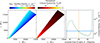 |
Fig. 7. Left and middle: wind density (left) and emissivity (right) profiles corresponding to the best fit XWINDFE model fit to the XRISM-resolve data (Fig. 6). It is clear that the high density and emissivity regions are concentrated towards the base of the wind. However, some additional contributions from larger scale regions in the wind give the ‘narrow-er’ core seen in the line profile in Fig. 6. Right: column-density profile as a function of azimuth through the wind (green line). The drop at ∼50° corresponds to the point where sight-lines do not reach the outer radius of the wind, rather cutting through the central regions. The vertical dashed orange line indicates the observer inclination for NGC 4151, while the solid blue horizontal line indicates the column-density of the PCFABS component as inferred from the continuum fit. The agreement here is remarkable given that the XWINDFE fit did not use any prior constraints on line-of-sight column-density. |
5. Discussion and conclusions
We have developed a model for emission line profiles originating from a wind structure on BLR-like scales, XWIND, which we have made publicly available. Our approach gives a physically motivated model that can be easily fit to XRISM data, and in the future NewAthena.
There are a number of caveats. Perhaps the most important being that we assume neutral material. This is unlikely to be the case for material surrounding an AGN, given the highly ionising SED typically associated with the inner accretion flow. Given the wide range in wind density, one might expect a range of ionisation states throughout. This may affect the line profile, as even small changes in ionisation can shift or weaken the emitted line (e.g. Bianchi et al. 2005), which in the best case simply mildly smooth the line, in the worst case significantly alter the line shape. The magnitude of these effects depends on wind properties, placing some limits to model parameters within which the results can be trusted. While we do not calculate ionisation on the fly, we can make a rough estimate. Using the SED of NGC 4151 from Mahmoud & Done (2020) and the wind densities derived in Section 4.4 we arrive at ionisation parameters ranging from log10ξ ∼ 2.5 − 3.5 in the high emissivity regions, where ξ = Lion/(nHR2) and Lion is the integrated luminosity from 13.6 eV to 13.6 keV (1–1000 Ryd), following standard definitions (Ferland et al. 2017; Mehdipour et al. 2016). This is initially problematic, given that in this regime one expects a significant contribution from ionised species of iron (Mehdipour et al. 2016). However, this is to neglect clumping, which may increase the local density of the emitting material, and thus reduce the overall ionisation state. Xrism Collaboration (2025) showed conclusively a clumpy outflow in PDS 456 through absorption, although that is for a UFO wind where the models of Matzeu et al. (2022) and Luminari et al. (2024) are likely more appropriate. However, it is not be unreasonable to assume that clumping can extend to these slower BLR scale winds, especially given the presence of the low ionisation slow-moving absorption lines seen in Kraemer et al. (2006). As such, we caution the reader that this model is a first-order approximation both in terms of ignoring internal clumping, such that XWIND can be thought of as a volume-averaged approximation, and in terms of the ionisation state of the material, which is completely ignored. While increasing the local density through clumping can address some of the caveats, we caution that this model should not be used for material significantly inwards of the BLR (r ≲ 1000) where ionisation will almost certainly alter the line shape.
There is also the caveat of the simplified geometry and velocity profile. We have assumed that the material is always outflowing. However, this is likely not the case, especially given the rather low outflow velocity derived in Section 4. It may be expected that at some point the outflow fails and the material falls back down, as in, for example, the failed radiative outflow models of the BLR (Czerny & Hryniewicz 2011; Naddaf et al. 2021). The motion of this infalling material is likely to be somewhat more chaotic than the smooth outflowing wind assumed here, potentially providing some additional smoothing or narrow component to the model line profile. Of course, the total effect of this would depend somewhat on the column density of the intervening wind, as the wind inwards of this would still cast a shadow across any material falling back down. Nonetheless, we caution that a physically complete picture should include at least a non-outflowing component, and that XWIND only provides a method for adding in the wind.
Caveats aside, the model does give a statistically good fit to the data, while providing physical constraints on BLR-like winds. It is particularly promising that our model fits not only give launch radii consistent with those seen in previous XRISM analysis of NGC 4151 (Xrism Collaboration 2024; Xiang et al. 2025), but also provide reasonable mass-outflow rates compared to the mass-accretion rate for NGC 4151. However, we stress that this is only one viable explanation, and that there are likely other models that give equally good fits to these data.
XRISM has provided an unprecedented view of the X-ray emitting regions in astrophysical sources, and for AGN has allowed the characterisation of multiple components of the Fe-Kα emitting regions. These data are of sufficient quality that they warrant physical models in order to start characterising their actual structure. Our approach provides a step forward in this regard, giving a fast and simple, yet physical, model for BLR scale outflows. In the future we will start applying our model to a wider sample of XRISM observations of moderately accreting AGN, with the aim of understanding the structure of BLR-like outflows across the wider population.
Data availability
The XWIND model code is available via the corresponding author’s GitHub page (https://github.com/scotthgn). We release two version. One written exclusively in FORTRAN designed to be used with the XSPEC spectral fitting package (https://github.com/scotthgn/XWIND), and a PYTHON version designed to give more flexibility (and plotting options), referred to as PYXWIND (https://github.com/scotthgn/PyXWIND). Both the XRISM and NuSTAR data are publicly available via the HEASARC service, and were previously published in Xiang et al. (2025).
Acknowledgments
We thank the anonymous referee for their constructive comments, which improved the quality of this manuscript. We would like to thank the XRISM team for their work on the initial compilation and analysis of the high resolution data, which motivated this work. We would also like to thank Jon M. Miller for useful discussions, in particular on the NGC 4151 data. SH acknowledges support from an IFPU fellowship, as well as previous support from the Science and Technologies Facilities Council (STFC) through the studentship ST/W507428/1. CD acknowledges support from STFC through the grant ST/T000244/1. This work made use of the following software: XSPEC (Arnaud 1996), NUMPY (Harris et al. 2020), ASTROPY (Astropy Collaboration 2013, 2018, 2022), and meson.
References
- Anders, E., & Grevesse, N. 1989, Geochim. Cosmochim. Acta, 53, 197 [Google Scholar]
- Andonie, C., Bauer, F. E., Carraro, R., et al. 2022a, A&A, 664, A46 [NASA ADS] [CrossRef] [EDP Sciences] [Google Scholar]
- Andonie, C., Ricci, C., Paltani, S., et al. 2022b, MNRAS, 511, 5768 [NASA ADS] [CrossRef] [Google Scholar]
- Arnaud, K. A. 1996, ASP Conf. Ser., 101, 17 [Google Scholar]
- Astropy Collaboration (Robitaille, T. P., et al.) 2013, A&A, 558, A33 [NASA ADS] [CrossRef] [EDP Sciences] [Google Scholar]
- Astropy Collaboration (Price-Whelan, A. M., et al.) 2018, AJ, 156, 123 [Google Scholar]
- Astropy Collaboration (Price-Whelan, A. M., et al.) 2022, ApJ, 935, 167 [NASA ADS] [CrossRef] [Google Scholar]
- Begelman, M. C., & McKee, C. F. 1983, ApJ, 271, 89 [NASA ADS] [CrossRef] [Google Scholar]
- Begelman, M. C., McKee, C. F., & Shields, G. A. 1983, ApJ, 271, 70 [CrossRef] [Google Scholar]
- Behar, E. 2009, ApJ, 703, 1346 [NASA ADS] [CrossRef] [Google Scholar]
- Bianchi, S., Miniutti, G., Fabian, A. C., & Iwasawa, K. 2005, MNRAS, 360, 380 [Google Scholar]
- Bianchi, S., La Franca, F., Matt, G., et al. 2008, MNRAS, 389, L52 [NASA ADS] [Google Scholar]
- Bischetti, M., Piconcelli, E., Vietri, G., et al. 2017, A&A, 598, A122 [NASA ADS] [CrossRef] [EDP Sciences] [Google Scholar]
- Bischetti, M., Maiolino, R., Carniani, S., et al. 2019, A&A, 630, A59 [NASA ADS] [CrossRef] [EDP Sciences] [Google Scholar]
- Bischetti, M., Fiore, F., Feruglio, C., et al. 2023, ApJ, 952, 44 [NASA ADS] [CrossRef] [Google Scholar]
- Blandford, R. D., & Payne, D. G. 1982, MNRAS, 199, 883 [CrossRef] [Google Scholar]
- Bogensberger, D., Nakatani, Y., Yaqoob, T., et al. 2025, PASJ, 77, S209 [Google Scholar]
- Chen, K., Halpern, J. P., & Filippenko, A. V. 1989, ApJ, 339, 742 [NASA ADS] [CrossRef] [Google Scholar]
- Choi, H., Leighly, K. M., Terndrup, D. M., Gallagher, S. C., & Richards, G. T. 2020, ApJ, 891, 53 [NASA ADS] [CrossRef] [Google Scholar]
- Choi, H., Leighly, K. M., Terndrup, D. M., et al. 2022, ApJ, 937, 74 [NASA ADS] [CrossRef] [Google Scholar]
- Cunningham, C. T. 1975, ApJ, 202, 788 [NASA ADS] [CrossRef] [Google Scholar]
- Czerny, B., & Hryniewicz, K. 2011, A&A, 525, L8 [NASA ADS] [CrossRef] [EDP Sciences] [Google Scholar]
- De Rosa, G., Peterson, B. M., Ely, J., et al. 2015, ApJ, 806, 128 [NASA ADS] [CrossRef] [Google Scholar]
- Dehghanian, M., Ferland, G. J., Kriss, G. A., et al. 2019a, ApJ, 877, 119 [NASA ADS] [CrossRef] [Google Scholar]
- Dehghanian, M., Ferland, G. J., Peterson, B. M., et al. 2019b, ApJ, 882, L30 [NASA ADS] [CrossRef] [Google Scholar]
- Elvis, M., Wilkes, B. J., McDowell, J. C., et al. 1994, ApJS, 95, 1 [Google Scholar]
- Fabian, A. C., Rees, M. J., Stella, L., & White, N. E. 1989, MNRAS, 238, 729 [Google Scholar]
- Ferland, G. J., Chatzikos, M., Guzmán, F., et al. 2017, Rev. Mex. Astron. Astrofis., 53, 385 [NASA ADS] [Google Scholar]
- Feruglio, C., Fiore, F., Carniani, S., et al. 2015, A&A, 583, A99 [NASA ADS] [CrossRef] [EDP Sciences] [Google Scholar]
- Fiore, F., Feruglio, C., Shankar, F., et al. 2017, A&A, 601, A143 [NASA ADS] [CrossRef] [EDP Sciences] [Google Scholar]
- Fukumura, K., Kazanas, D., Contopoulos, I., & Behar, E. 2010, ApJ, 715, 636 [NASA ADS] [CrossRef] [Google Scholar]
- Fukumura, K., Kazanas, D., Shrader, C., et al. 2017, Nat. Astron., 1, 0062 [NASA ADS] [CrossRef] [Google Scholar]
- Amorim, A. 2024, A&A, 684, A167 [NASA ADS] [CrossRef] [EDP Sciences] [Google Scholar]
- GRAVITY Collaboration (Abd El Dayem, K., et al.) 2026, A&A, 706, A99 [Google Scholar]
- Haardt, F., & Maraschi, L. 1993, ApJ, 413, 507 [Google Scholar]
- Haardt, F., Maraschi, L., & Ghisellini, G. 1994, ApJ, 432, L95 [NASA ADS] [CrossRef] [Google Scholar]
- Hagino, K., Odaka, H., Done, C., et al. 2015, MNRAS, 446, 663 [NASA ADS] [CrossRef] [Google Scholar]
- Hagino, K., Odaka, H., Done, C., et al. 2016, MNRAS, 461, 3954 [Google Scholar]
- Harris, C. R., Millman, K. J., van der Walt, S. J., et al. 2020, Nature, 585, 357 [NASA ADS] [CrossRef] [Google Scholar]
- Higginbottom, N., Knigge, C., Long, K. S., et al. 2018, MNRAS, 479, 3651 [NASA ADS] [CrossRef] [Google Scholar]
- Hölzer, G., Fritsch, M., Deutsch, M., Härtwig, J., & Förster, E. 1997, Phys. Rev. A, 56, 4554 [CrossRef] [Google Scholar]
- Igo, Z., Parker, M. L., Matzeu, G. A., et al. 2020, MNRAS, 493, 1088 [NASA ADS] [CrossRef] [Google Scholar]
- Kammoun, E., Kawamuro, T., Murakami, K., et al. 2025, ApJ, 994, L13 [Google Scholar]
- Kara, E., Mehdipour, M., Kriss, G. A., et al. 2021, ApJ, 922, 151 [NASA ADS] [CrossRef] [Google Scholar]
- Kelley, R. L., Ishisaki, Y., Costantini, E., et al. 2025, J. Astron. Telesc. Instrum. Syst., 11, 042026 [Google Scholar]
- King, A. R. 2010, MNRAS, 402, 1516 [Google Scholar]
- Knigge, C., Woods, J. A., & Drew, J. E. 1995, MNRAS, 273, 225 [NASA ADS] [Google Scholar]
- Kraemer, S. B., Crenshaw, D. M., Gabel, J. R., et al. 2006, ApJS, 167, 161 [Google Scholar]
- Leighly, K. M., Hamann, F., Casebeer, D. A., & Grupe, D. 2009, ApJ, 701, 176 [Google Scholar]
- Leighly, K. M., Terndrup, D. M., Gallagher, S. C., Richards, G. T., & Dietrich, M. 2018, ApJ, 866, 7 [NASA ADS] [CrossRef] [Google Scholar]
- Lindquist, R. W. 1966, Ann. Phys., 37, 487 [NASA ADS] [CrossRef] [Google Scholar]
- Long, K. S., & Knigge, C. 2002, ApJ, 579, 725 [NASA ADS] [CrossRef] [Google Scholar]
- Luminari, A., Piconcelli, E., Tombesi, F., et al. 2018, A&A, 619, A149 [NASA ADS] [CrossRef] [EDP Sciences] [Google Scholar]
- Luminari, A., Nicastro, F., Krongold, Y., Piro, L., & Thakur, A. L. 2023, A&A, 679, A141 [NASA ADS] [CrossRef] [EDP Sciences] [Google Scholar]
- Luminari, A., Piconcelli, E., Tombesi, F., Nicastro, F., & Fiore, F. 2024, A&A, 691, A357 [NASA ADS] [CrossRef] [EDP Sciences] [Google Scholar]
- Luminet, J. P. 1979, A&A, 75, 228 [Google Scholar]
- Lusso, E., & Risaliti, G. 2016, ApJ, 819, 154 [Google Scholar]
- Magdziarz, P., & Zdziarski, A. A. 1995, MNRAS, 273, 837 [Google Scholar]
- Mahmoud, R. D., & Done, C. 2020, MNRAS, 491, 5126 [NASA ADS] [Google Scholar]
- Maiolino, R., Gallerani, S., Neri, R., et al. 2012, MNRAS, 425, L66 [Google Scholar]
- Matthews, J. H., Long, K. S., Knigge, C., et al. 2025, MNRAS, 536, 879 [Google Scholar]
- Matzeu, G. A., Reeves, J. N., Braito, V., et al. 2017, MNRAS, 472, L15 [NASA ADS] [CrossRef] [Google Scholar]
- Matzeu, G. A., Lieu, M., Costa, M. T., et al. 2022, MNRAS, 515, 6172 [NASA ADS] [CrossRef] [Google Scholar]
- Mehdipour, M., Kaastra, J. S., & Kallman, T. 2016, A&A, 596, A65 [NASA ADS] [CrossRef] [EDP Sciences] [Google Scholar]
- Mehdipour, M., Kaastra, J. S., Eckart, M. E., et al. 2025, A&A, 699, A228 [NASA ADS] [CrossRef] [EDP Sciences] [Google Scholar]
- Miller, J. M., Cackett, E., Zoghbi, A., et al. 2018, ApJ, 865, 97 [Google Scholar]
- Miller, J. M., Xiang, X., Byun, D., et al. 2025, ApJ, 994, L10 [Google Scholar]
- Murphy, K. D., & Yaqoob, T. 2009, MNRAS, 397, 1549 [Google Scholar]
- Naddaf, M.-H., Czerny, B., & Szczerba, R. 2021, ApJ, 920, 30 [NASA ADS] [CrossRef] [Google Scholar]
- Nandra, K., O’Neill, P. M., George, I. M., & Reeves, J. N. 2007, MNRAS, 382, 194 [NASA ADS] [CrossRef] [Google Scholar]
- Nardini, E., Reeves, J. N., Gofford, J., et al. 2015, Science, 347, 860 [Google Scholar]
- Noda, H., Mineta, T., Minezaki, T., et al. 2023, ApJ, 943, 63 [NASA ADS] [CrossRef] [Google Scholar]
- Noda, H., Mori, K., Tomida, H., et al. 2025a, PASJ, 77, S10 [Google Scholar]
- Noda, H., Yamada, S., Ogawa, S., et al. 2025b, ApJ, 993, L53 [Google Scholar]
- Nomura, M., & Ohsuga, K. 2017, MNRAS, 465, 2873 [Google Scholar]
- Nomura, M., Ohsuga, K., Takahashi, H. R., Wada, K., & Yoshida, T. 2016, PASJ, 68, 16 [NASA ADS] [CrossRef] [Google Scholar]
- Odaka, H., Aharonian, F., Watanabe, S., et al. 2011, ApJ, 740, 103 [NASA ADS] [CrossRef] [Google Scholar]
- Proga, D., & Kallman, T. R. 2004, ApJ, 616, 688 [Google Scholar]
- Proga, D., Stone, J. M., & Kallman, T. R. 2000, ApJ, 543, 686 [Google Scholar]
- Reeves, J. N., O’Brien, P. T., Braito, V., et al. 2009, ApJ, 701, 493 [NASA ADS] [CrossRef] [Google Scholar]
- Shakura, N. I., & Sunyaev, R. A. 1973, A&A, 24, 337 [NASA ADS] [Google Scholar]
- Sim, S. A., Long, K. S., Miller, L., & Turner, T. J. 2008, MNRAS, 388, 611 [CrossRef] [Google Scholar]
- Tombesi, F., Cappi, M., Reeves, J. N., et al. 2010, A&A, 521, A57 [NASA ADS] [CrossRef] [EDP Sciences] [Google Scholar]
- Tzanavaris, P., Yaqoob, T., & LaMassa, S. 2023, Phys. Rev. D, 108, 123037 [Google Scholar]
- Vander Meulen, B., Camps, P., Stalevski, M., & Baes, M. 2023, A&A, 674, A123 [NASA ADS] [CrossRef] [EDP Sciences] [Google Scholar]
- Weymann, R. J., Morris, S. L., Foltz, C. B., & Hewett, P. C. 1991, ApJ, 373, 23 [NASA ADS] [CrossRef] [Google Scholar]
- Wilms, J., Allen, A., & McCray, R. 2000, ApJ, 542, 914 [Google Scholar]
- Xiang, X., Miller, J. M., Behar, E., et al. 2025, ApJ, 988, L54 [Google Scholar]
- Xrism Collaboration (Audard, M., et al.) 2024, ApJ, 973, L25 [Google Scholar]
- Xrism Collaboration (Audard, M., et al.) 2025, Nature, 641, 1132 [Google Scholar]
- Yaqoob, T. 2012, MNRAS, 423, 3360 [Google Scholar]
- Yaqoob, T. 2024, MNRAS, 527, 1093 [Google Scholar]
- Yaqoob, T., & Padmanabhan, U. 2004, ApJ, 604, 63 [NASA ADS] [CrossRef] [Google Scholar]
- Yaqoob, T., George, I. M., Nandra, K., et al. 2001, ApJ, 546, 759 [Google Scholar]
Appendix A: XWIND model documentation
We release both an XSPEC version of XWIND, written in FORTRAN, as well as a stand-alone PYTHON version, PYXWIND, for use-cases outside of XSPEC. Within XWIND we release three model flavours: XWINDLINE, XWINDFE, and XWINDCONV. Here we give a brief overview of each model flavour. We note that PYXWIND includes additional functionality for plotting and the calculation of column-density profiles. For these details we refer the reader to the documentation on the GitHub page: https://github.com/scotthgn/PyXWIND.
XWINDLINE: This is the base model, which simply focuses on the line-shape as given by the wind. As such the rest-frame energy is treated as a free parameter, and the rest-frame emission is considered a simple delta-function. Here the normalisation should also be treated as a free parameter, as the model does not consider the output equivalent width. The input parameters for XWINDLINE are given in table A.1.
XWIND model parameter
XWINDFE: This model is specific to the Fe-Kα complex. As such it calculates self-consistently the equivalent width of the emission line (see section 3.2), and so the normalisation in XSPEC should always be fixed at unity. The absolute line flux is instead set by the number of photons absorbed, and re-emitted, by the wind, which is fundamentally governed by the density profile as well as the incident X-ray spectrum originating from the central corona. Hence, the model takes as input parameters the normalisation and photon index of the incident spectrum. These should always be tied to a corresponding fit of the broad-band continuum, and not left free while fitting the line-profile. In addition to the self-consistent normalisation, XWINDFE uses the 7-Lorentzian Hölzer et al. (1997) profile for the rest-frame emission. This leads to it naturally including Lorentzian wings, as well as both Fe-Kα1 and Fe-Kα2 lines. The input parameters for this model are given in tabel A.2.
XWINDFE model parameters
XWINDCONV: Convolution model. Takes the line-profiles from XWINDLINE, and uses them as a convolution kernel that is the applied to some input spectrum. Note that the normalisation used is such that the convolution conserves the photon number of the input spectrum (i.e if you convolve an input spectrum containing 100 photons with XWINDCONV the output spectrum will also contain 100 photons). The advantage here is that one can apply wind broadening to either continuum emission (e.g the diffuse continuum, under certain assumptions) or output line emission from e.g more realistic radiative transfer calculations (from e.g CLOUDY Ferland et al. 2017), again under the assumption that the emissivity follows the profile calculated here. The input parameters are given in table A.3.
XWINDCONV model parameters
Appendix B: Comparison to DISKLINE
As a sanity check we, we adapt our model to a Keplerian disc, allowing for a direct comparison to the well established DISKLINE (Fabian et al. 1989). The main differences from XWIND are that we now only consider the Keplerian velocity component in Eqn. 15 (as well as the gravitational redshift). We also calculate the emission using a simple radial emissivity profile, with ϵ(r)∝r−3.
The resulting line-profiles are shown in Fig. B.1, where we have performed comparisons while stepping through inner radius (left panel), and observer inclination (middle and right panels). DISKLINE is shown as the dashed black lines, while the profile from our code is shown as the solid coloured lines. For large radii, r ≳ 50, the profiles are entirely consistent with one another. This is not the case at small radii where we start to see some systematic deviation. This is likely due to out choice of a flat-space time metric. While DISKLINE ignores light-bending, it does still calculate the energy shifts and impact parameters in the Schwarzchild metric. This becomes important at small radii. As such, we do not recommend the use of our model for very small launch radii (as might be expected from e.g. at UFO type wind).
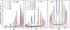 |
Fig. B.1. Comparison of line profiles for a Keplerian disc, calculated considering only relativistic Doppler shifts as outlined in section 2.5 (solid coloured lines) and calculated using the DISKLINE model (Fabian et al. 1989) (dashed lines), which includes some corrections expected from the Schwarzchild metric. In all cases these are calculated for a narrow annulus, such that rout = 1.1rin. The left panel shows the profiles while stepping through values of rin, in order to highlight where our approximations break down. For rin ≳ 50 our line profile matches that or DISKLINE well, whereas below this we start to see systematic offsets originating from our choice of metric. The middle and right panels show the profiles while stepping through observed inclination, with rin = 20 and 200 respectively. Again, in the weak field limit, where general relativistic corrections are small, our approximation matches well that of DISKLINE. |
Nonetheless, at BLR scales, the general relativistic corrections are negligible, with perhaps the exception of the gravitational redshift, which is included in our model.
Appendix C: Line-profile component tests
We present here a brief set of comparison fits to quantitate the significance of each component. In total we perform six additional fits, removing/including the XWINDFE, MYTOURS, and DISKLINE components. The underlying continuum model is fixed to that presented in section 4. As with our fiducial model fit, we use the 5.0 − 6.6 keV range of the XRISM-resolve spectrum. The resulting fits are shown in Fig. C.1, with a a zoom in on the residual shown in Fig. C.2. Each panel in the figures gives the relevant model combination to the line profile.
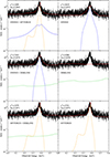 |
Fig. C.1. Model fits to XRISM-resolve for subsets of our total line-profile model, to highlight the significance of each component. As with the main model in Fig. 6 these have been fit over the 5.0-6.6 keV energy range. The left column shows the case for a two-component model to the Fe-Kα complex, while the right shows a single component scenario. The relevant model components (shown as dashed coloured lines) are XWINDFE (blue), MYTORUS (orange), and DISKLINE (green). In all cases, these result in a statistically significantly worse fit than our fiducial three component model for the Fe-Kα complex. |
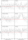 |
Fig. C.2. Residual to the fits presented in Fig. C.1. Note we have chosen to zoom in on the 6.25-6.5 keV region in order to highlight the residuals around the Fe-Kα complex. The fits, however, are performed across the 5.0-6.6 keV range. |
Perhaps the least significant component to the line profile is DISKLINE, with Δχ2 = 75 with only 2 additional degrees of freedom. This is not particularly surprising, given that broad components suffer from dilution with the underlying continuum, especially in high resolution spectra.
More importantly for this paper, we see that both the MYTORUS and XWINDFE components are significant, with Δχ2 = 109 and Δχ2 = 145 for 3 and 4 additional degrees of freedom, respectively. It is quite clear in the residuals shown in Fig. C.2 that these components are required to model the narrow and intermediary components of the line.
All Tables
Best fit parameters for the model fit to the Fe-Kα complex in the XRISM-Resolve spectrum.
All Figures
|
Fig. 1. Left: definition of our model geometry. The wind is launched between rin and rout, at an angle defined by the distance of the focus below the origin, df. The covering fraction fcov defines the maximum radial extent of the wind rmax (in spherical polar coordinates), giving a spherical boundary condition. Right: example of our calculation grid (at significantly lower resolution for clarity). We split the wind into cells of cos(θ) with width dcos(θ) in the range cos(θ)∈[0, fcov], and radius r with width dlog(r). The grid in r extends from the inner streamline to either the outer streamline (defined from rout) or rmax, depending on whichever is smallest. Our wind cells are illustrated as the dark shaded regions. Throughout this paper we will evaluate the wind emission and density at the centre of each cell θi and rj. For completeness, this also defines the length travelled along the streamline lij at each cell. |
| In the text | |
|
Fig. 2. Wind density profile (left column) and corresponding emissivity profile (middle column) for a range of outflow velocities (increasing from top to bottom, value given in top left corner of each row). The right column shows the column-density profile for varying lines of sight through the winds. These have all been calculated for a wind launched between rin = 1000 and rout = 3000, with |
| In the text | |
|
Fig. 3. Example emission line profiles and their evolution with varying wind parameters. These have all been re-normalised to have the same total flux, and have all been calculated for an observed inclination of 45 degrees. Each panel shows the effect of varying an individual parameter, given in the top left corner of each panel. When not being varied, parameters are fixed at: ṁw= 10−2, rin = 700, rout = 3rin, |
| In the text | |
|
Fig. 4. Left: colour-plot showing the equivalent width of the Fe-Kα emission line for varying ṁw and v∞. The darker the shade of green, the larger the equivalent width. The vertical, horizontal solid, and dashed lines correspond to the slices used to extract the curves of growth on the right as a function of ṁw/v∞. Right: curves of growth as a function of ṁw (left panel) and v∞ (right panel). As ṁw increases, so does the equivalent width, until eventually the line saturates due to the wind becoming optically thick. Conversely, increasing v∞ will reduce the equivalent width, as this reduces the overall density of the wind (see Fig. 2) leading to a lower degree of absorption and thus fewer photons available to re-emit as Fe-Kα. |
| In the text | |
|
Fig. 5. Best fit broad-band continuum, using combined XRISM-xtend (black crosses) and NuSTAR (orange and grey crosses for FPMA and FPMB respectively).The solid red line shows the total spectral model, with the dotted and dashed lines showing the individual components. These are: the scattered continuum (dotted blue), reflection spectrum (dashed magenta), and the primary continuum (dashed-dotted blue). The plotted NuSTAR data have been corrected by a cross-calibration constant used to account for instrumental differences between XRISM-xtend and NuSTAR. The data have been re-binned slightly for clarity. |
| In the text | |
|
Fig. 6. Top: best fit model to XRISM-resolve data (black points). The solid red line shows the total model, while the dashed and dotted lines show the components. These are: scattered and primary continuum (grey dotted lines), MYTORUS emission line from Compton thick slow-moving material (orange dashed line), XWINDFE emission line for a wind inwards of the BLR (blue dashed line), and DISKLINE emission line from the inner disc (green dashed line). Bottom: data-model residuals, normalised by the data errorbar. The shaded blue bands show the 1σ (dark) and 2σ (light) deviation. |
| In the text | |
|
Fig. 7. Left and middle: wind density (left) and emissivity (right) profiles corresponding to the best fit XWINDFE model fit to the XRISM-resolve data (Fig. 6). It is clear that the high density and emissivity regions are concentrated towards the base of the wind. However, some additional contributions from larger scale regions in the wind give the ‘narrow-er’ core seen in the line profile in Fig. 6. Right: column-density profile as a function of azimuth through the wind (green line). The drop at ∼50° corresponds to the point where sight-lines do not reach the outer radius of the wind, rather cutting through the central regions. The vertical dashed orange line indicates the observer inclination for NGC 4151, while the solid blue horizontal line indicates the column-density of the PCFABS component as inferred from the continuum fit. The agreement here is remarkable given that the XWINDFE fit did not use any prior constraints on line-of-sight column-density. |
| In the text | |
|
Fig. B.1. Comparison of line profiles for a Keplerian disc, calculated considering only relativistic Doppler shifts as outlined in section 2.5 (solid coloured lines) and calculated using the DISKLINE model (Fabian et al. 1989) (dashed lines), which includes some corrections expected from the Schwarzchild metric. In all cases these are calculated for a narrow annulus, such that rout = 1.1rin. The left panel shows the profiles while stepping through values of rin, in order to highlight where our approximations break down. For rin ≳ 50 our line profile matches that or DISKLINE well, whereas below this we start to see systematic offsets originating from our choice of metric. The middle and right panels show the profiles while stepping through observed inclination, with rin = 20 and 200 respectively. Again, in the weak field limit, where general relativistic corrections are small, our approximation matches well that of DISKLINE. |
| In the text | |
|
Fig. C.1. Model fits to XRISM-resolve for subsets of our total line-profile model, to highlight the significance of each component. As with the main model in Fig. 6 these have been fit over the 5.0-6.6 keV energy range. The left column shows the case for a two-component model to the Fe-Kα complex, while the right shows a single component scenario. The relevant model components (shown as dashed coloured lines) are XWINDFE (blue), MYTORUS (orange), and DISKLINE (green). In all cases, these result in a statistically significantly worse fit than our fiducial three component model for the Fe-Kα complex. |
| In the text | |
|
Fig. C.2. Residual to the fits presented in Fig. C.1. Note we have chosen to zoom in on the 6.25-6.5 keV region in order to highlight the residuals around the Fe-Kα complex. The fits, however, are performed across the 5.0-6.6 keV range. |
| In the text | |
Current usage metrics show cumulative count of Article Views (full-text article views including HTML views, PDF and ePub downloads, according to the available data) and Abstracts Views on Vision4Press platform.
Data correspond to usage on the plateform after 2015. The current usage metrics is available 48-96 hours after online publication and is updated daily on week days.
Initial download of the metrics may take a while.