| Issue |
A&A
Volume 710, June 2026
|
|
|---|---|---|
| Article Number | A33 | |
| Number of page(s) | 21 | |
| Section | Stellar structure and evolution | |
| DOI | https://doi.org/10.1051/0004-6361/202557843 | |
| Published online | 29 May 2026 | |
SN 2024iss: A double-peaked Type IIb supernova with evidence of circumstellar interaction
1
Department of Physics, Tsinghua University, Beijing 100084, China
2
National Astronomical Observatories, Chinese Academy of Sciences, Beijing 100101, China
3
School of Astronomy and Space Science, University of Chinese Academy of Sciences, Beijing 100049,1408, China
4
Las Cumbres Observatory, 6740 Cortona Drive, Suite 102 Goleta, CA 93117, USA
5
Department of Physics, University of California Santa Barbara, Santa Barbara, California 93106, USA
6
Università degli Studi di Padova, Dipartimento di Fisica e Astronomia, Vicolo dell’Osservatorio 2, 35122 Padova, Italy
7
INAF – Osservatorio Astronomico di Padova, Vicolo dell’Osservatorio 5, 35122 Padova, Italy
8
INAF – Osservatorio Astronomico di Brera, Via Bianchi 46, 23807 Merate, (LC), Italy
9
Department of Astronomy, University of California, Berkeley, CA 94720-3411, USA
10
Yunnan Observatories, Chinese Academy of Sciences, Kunming 650216, China
11
International Centre of Supernovae, Yunnan Key Laboratory, Kunming 650216, China
12
Key Laboratory for the Structure and Evolution of Celestial Objects, Chinese Academy of Sciences, Kunming 650216, China
13
Steward Observatory, University of Arizona, 933 North Cherry Avenue, Tucson, AZ 85721-0065, USA
14
Gemini Observatory, 670 North A‘ohoku Place, Hilo, HI 96720-2700, USA
15
Xinjiang Astronomical Observatory, Chinese Academy of Sciences, Urumqi, Xinjiang 830011, China
16
Università degli Studi di Padova, Dipartimento di Fisica e Astronomia, Vicolo dell’Osservatorio 3, 35122 Padova, Italy
17
Key Laboratory of Optical Astronomy, National Astronomical Observatories, Chinese Academy of Sciences, Beijing 100101, China
18
Department of Astronomy, University of Texas, Austin, TX 78712, USA
19
Kavli Institute for Theoretical Physics, University of California, Santa Barbara, 552 University Road, Goleta, CA 93106-4030, USA
20
Johns Hopkins University, Baltimore, MD, USA
21
School of Physics and Astronomy, Monash University, Clayton, Australia
22
OzGrav: The ARC Center of Excellence for Gravitational Wave Discovery, Hawthorn, VIC 3122, Australia
23
Adler Planetarium, 1300 S. DuSable Lake Shore Dr., Chicago, IL 60605, USA
24
HUN-REN CSFK Konkoly Observatory, MTA Center of Excellence, Konkoly Thege ut 15-17 Budapest 1121, Hungary
25
Department of Experimental Physics, University of Szeged, Dóm tér 9 Szeged 6720, Hungary
26
ELTE Eötvös Loránd University, Institute of Physics and Astronomy, Pázmány Péter sétány 1/A, Budapest 1117, Hungary
27
Institute of High Energy Physics, Chinese Academy of Sciences, Beijing 100049, China
28
Beijing Planetarium, Beijing Academy of Sciences and Technology, Beijing 100044, China
★ Corresponding authors: This email address is being protected from spambots. You need JavaScript enabled to view it.
, This email address is being protected from spambots. You need JavaScript enabled to view it.
Received:
27
October
2025
Accepted:
5
February
2026
Abstract
Aims. We present optical, ultraviolet, and X-ray observations of supernova (SN) 2024iss, a Type IIb SN that shows a prominent double-peaked light curve.
Methods. We modeled the first peak with a semianalytical shock-cooling model and the X-ray emission with a free-free model. We also compared the envelope radius and mass-loss rate with those of other Type IIb SNe to explore the relationships between the progenitor envelope and the circumstellar material.
Results. The shock-cooling peak in the V-band light curve reached MV = −17.33 ± 0.26 mag, while the 56Ni-powered second peak attained MV = −17.43 ± 0.26 mag. Early spectra show a photospheric velocity of approximately 19 400 km s−1 at 3.82 days from the Hα P Cygni profile. The Balmer lines persist for at least more than 87 days after the explosion, which is characteristic of hydrogen-rich ejecta. Modeling the first light-curve peak with the shock-cooling model suggests an extended hydrogen envelope with a mass of 0.11 ± 0.04 M⊙ and a radius of 244 ± 43 R⊙. Fitting the second light-curve peak with an Arnett-like model indicates a typical 56Ni mass of 0.117 ± 0.013 M⊙ and a relatively low ejecta mass of 1.27 ± 0.34 M⊙. X-ray observations revealed bright thermal bremsstrahlung emission and indicate a mass-loss rate of 1.6 × 10⁻⁵ M⊙ yr−1, which is similar to that of SN 1993J.
Conclusions. Supernova 2024iss occupies a transitional position between the two subclasses of extended and compact Type IIb SNe. Its envelope radius and preexplosion mass-loss rate appear to be consistent with the correlation observed in the broader sample. The observational properties of SN 2024iss are compatible with a binary-interaction scenario being the dominant mechanism for envelope stripping.
Key words: stars: massive / stars: mass-loss / supernovae: individual: SN2024iss
LSSTC Catalyst Fellow.
© The Authors 2026
 Open Access article, published by EDP Sciences, under the terms of the Creative Commons Attribution License (https://creativecommons.org/licenses/by/4.0), which permits unrestricted use, distribution, and reproduction in any medium, provided the original work is properly cited.
This article is published in open access under the Subscribe to Open model. This email address is being protected from spambots. You need JavaScript enabled to view it. to support open access publication.
1. Introduction
Type IIb supernovae (SNe) are generally thought to form a transitional subclass whose spectroscopic properties lie between those of the Type II and Ib SNe (for reviews, see Filippenko 1997; Gal-Yam 2017). The spectra of Type IIb SNe initially exhibit strong hydrogen features with no evidence of helium. The hydrogen lines persist only for the first few weeks after explosion, after which P-Cygni features of He I begin to appear in the spectra (see, e.g., Filippenko 1997).
The rather prompt emergence of helium lines indicates that the outermost envelope of the progenitors of Type IIb SNe has been partially stripped, thus providing an important approach to test the mechanisms that can dramatically strip the outer envelopes of massive progenitor stars. The remarkable transformation between the hydrogen- and helium-dominated spectroscopic phases was initially revealed by the extensive observing campaign on SN 1993J (Filippenko et al. 1993, 1994; Woosley et al. 1994; Barbon et al. 1995; Richmond et al. 1996; Matheson et al. 2000). Thanks to the transient-alert stream produced by high-cadence wide-field sky surveys such as the Palomar Transient Factory (PTF; Rau et al. 2009; Law et al. 2009) and later the Zwicky Transient Facilities (Bellm et al. 2019; Graham et al. 2019), large samples of SNe IIb have been studied, including SNe 2011dh (Arcavi et al. 2011; Ergon et al. 2014), 2011fu (Kumar et al. 2013; Morales-Garoffolo et al. 2015), 2013df (Morales-Garoffolo et al. 2014; Szalai et al. 2016), 2016gkg (Tartaglia et al. 2017; Bersten et al. 2018; Sravan et al. 2018), 2017ati (Peng et al. 2026), 2017ckj (Li et al. 2025), 2020acat (Medler et al. 2022), 2022ngb (Zhao et al. 2026) and 2024uwq (Subrayan et al. 2025). Detailed analyses of the homogeneity and diversity of SNe IIb have also been performed based on larger samples (e.g., Shivvers et al. 2019).
One way to investigate the nature of Type IIb SNe can be facilitated by analyzing archival preexplosion images. By fitting stellar evolutionary tracks to the spectral energy distribution (SED) extracted at the exact location of the SN in the archival images taken by the Hubble Space Telescope (HST), various studies have suggested that the progenitor stars of SNe IIb tend to be yellow (or even cooler) supergiants. Examples include SNe 1993J (Maund et al. 2004), 2013df (Van Dyk et al. 2014), 2016gkg (Kilpatrick et al. 2017; Tartaglia et al. 2017), 2017gkk (Niu et al. 2024) and 2024abfo (Reguitti et al. 2025; Niu et al. 2025).
A more general approach to investigating the nature of the progenitor can be achieved by fitting the early-time emissions of the SN explosion with a shock-cooling model. This process characterizes the energy emitted by the shock breakout deposited in the ejecta and describes how such energy diffuses out as the ejecta expand and cool (see, e.g., Waxman et al. 2017 for a review). The early luminosity evolution of SNe IIb often manifests itself as a double-peaked light curve, where the first peak is powered by the cooling of the extended envelope of the progenitor star heated by the shock, called the shock-cooling emission (Soderberg et al. 2012). Various semi-analytic models have been developed within the framework of shock cooling and were used to fit the early light curves of core-collapse (CC) SNe.
Piro et al. (2021) introduced a two-zone model with a broken power law to characterize the radial density structure of the envelope. This model builds on the earlier works of Piro (2015) and Nakar & Piro (2014). Meanwhile, Sapir & Waxman (2017) extended the earlier work of Rabinak & Waxman (2011) to a longer regime of validity, introducing two choices of the polytropic index: n = 3 for radiative envelopes (e.g., blue supergiants) and n = 3/2 for convective envelopes (e.g., red supergiants). Morag et al. (2023) further developed the framework of Sapir & Waxman (2017) by considering the effects of strong blanketing of numerous iron absorption lines in the near-ultraviolet (UV) to optical wavelength ranges and the multizone dynamics, increasing the feasibility of the model at early phases. Farah et al. (2025b) developed a framework for shock-cooling fitting of SNe IIb, employing various models to constrain the envelope mass and radius. Moreover, Nagy & Vinkó (2016) developed a semi-analytical model to constrain the nature of the envelope by considering a dense inner region and an extended low-mass envelope.
These models of the early luminosity evolution of SNe IIb generally suggest that the extended hydrogen envelope associated with their first light-curve peak have masses of 10−2–10−1 M⊙ and radii of 100–500 R⊙, which are both broadly consistent with the results of preexplosion imaging, although some discrepancies remain unresolved. Alternative interpretations of the early light curve peak have also been proposed, including a bimodal radial distribution of [56]Ni (Orellana & Bersten 2022) and thermal energy deposited by the shock as it propagates through the envelope (Liu et al. 2025).
Owing to preexplosion mass loss and partial envelope stripping, some SNe IIb also exhibit signatures of circumstellar material (CSM), offering valuable insights into the preexplosion mass-loss history of their progenitor systems (Smith 2017). X-ray emission provides an important trace of the ejecta-CSM interaction. Fransson et al. (1996) analyzed the X-ray emission of SN 1993J and attributed it to the thermal bremsstrahlung produced by the forward shock. This framework was extended in studies of SNe 2011dh (Soderberg et al. 2012) and 2013df (Kamble et al. 2016) and led to further support of the role of X-ray observations in providing critical constraints on the electron number density of the CSM around Type IIb SNe. Dwarkadas (2025) compiled the early X-ray light curves of interacting CCSNe and found no compelling evidence for nonthermal X-ray emission in SNe IIb.
The mechanism stripping the envelopes of the progenitor star remains uncertain. The removal of the progenitor’s envelope and the formation of CSM generally result from two scenarios: single-star or binary-interaction mechanisms. In the framework of wind-driven mass loss (e.g., Woosley et al. 1993; Georgy 2012; Yoon 2017), the stripping of a star can be rather intense and may indicate a massive progenitor such as a Wolf-Rayet star, as seen in events such as the first broad-line SN IIb (Hamuy et al. 2009). Additionally, eruptive mass loss just prior to the terminal explosion may be triggered by processes including pulsation-driven superwinds (Yoon & Cantiello 2010) or core neutrino emission (Moriya 2014).
Alternatively, binary interaction has gained increasing support in recent years as a more prevalent explanation for envelope stripping (Podsiadlowski 1992; Smith 2014; Sravan et al. 2020; Dessart et al. 2024). Sana et al. (2012) indicates that more than 70% of massive stars undergo mass exchange with a companion, with about one-third resulting in binary mergers. Direct imaging has confirmed companion stars in some Type IIb SN progenitors, such as those of SN 1993J (Maund & Smartt 2009) and SN 2001ig (Ryder et al. 2018). Furthermore, binary scenarios naturally explain the observed correlations between CSM properties and the residual envelope of the progenitor.
Chevalier & Soderberg (2010) were the first to classify SNe IIb into two subtypes based on the prominence of their shock-cooling emission, and the authors investigated the associated X-ray properties. The extended subtype (Type eIIb) exhibits a pronounced shock-cooling peak in the early-time light curve, indicating a relatively massive hydrogen envelope (≥0.1 M⊙) and a large progenitor radius (∼100–1000 R⊙). These events typically show thermal X-ray emission. In contrast, objects belonging to the compact subtype (Type cIIb) display a weaker or no signature of shock cooling, indicating smaller sizes of their progenitors.
Following this classification, Soderberg et al. (2012) and Kamble et al. (2016) found that Type eIIb SNe generally exhibit stronger X-ray emission and are surrounded by denser CSM. The distinction between Type eIIb and Type cIIb is further supported by Maeda et al. (2015) and Ouchi & Maeda (2017), who showed that the initial orbital separation affects the residual envelope mass and preexplosion mass loss. In this framework, closer binaries tend to produce more stripped, compact progenitors with lower mass-loss rates. A parallel study by Yoon et al. (2017) proposed that Type eIIb SNe originate from systems undergoing late Case B mass transfer and evolve into red supergiants, while Type cIIb events would result from early Case B transfer and evolve into blue supergiants or yellow supergiants. Nevertheless, the sample size of SNe IIb is still limited, and events with comprehensive optical and X-ray observations are even sparser. Further studies of the relationship between the envelope and the CSM will require a larger well-characterized sample.
In this article, we present and analyze spectrophotometric and X-ray observations of SN 2024iss, a nearby Type IIb SN with a prominent double peak in optical bands and exhibiting bright thermal X-ray emission comparable to that of SN 1993J. Basic information about SN 2024iss is provided in Section 2.1. The details of the observations and data reduction are described in Section 2. In Section 3, we analyze the multiband light curves and the evolution of the pseudobolometric luminosity. The spectral evolution and comparisons with other well-observed SNe IIb are discussed in Section 4. In Section 5, we model the early shock-cooling emission peak. The X-ray properties are inferred in Section 6. In Section 7 we discuss possible mass-loss mechanisms for SN 2024iss. Our main conclusions are summarized in Section 8.
2. Observations and data reduction
2.1. Discovery and host galaxy
SN 2024iss was discovered on UTC 2024 May 12, 21:37 (MJD 60442.901) by the Gravitational-wave Optical Transient Observer (GOTO; Steeghs et al. 2022). Approximately six hours before the reported discovery, the SN emission was recorded by a public-outreach telescope located at the Xinglong Observatory, as detailed in Section 2. The SN exploded at J2000 celestial coordinates  ,
,  , in the outskirts of the nearby dwarf galaxy WISEA J125906.48+284842.6 (redshift z = 0.003334). This is in contrast to the sample of SNe IIb in Ma et al. (2025), where the majority of the host galaxies are spirals. Moreover, the host galaxy of SN 2024iss is also dimmer than most of those of well-studied SNe IIb, with W1 = −15.56 ± 0.62 mag.
Assuming a flat Λ cold dark matter (ΛCDM) model with H0 = 73.0 km s−1 Mpc−1, Ωm = 0.27, and ΩΛ = 0.73 (Spergel et al. 2007), we adopt a distance of 13.4 ± 1.6 Mpc, based on the Local Group velocity (Fixsen et al. 1996), as acquired from the NASA/IPAC Extragalactic Database (NED).
Considering the low redshift of SN 2024iss, we adopted an additional 10% uncertainty in distance to account for the effect of the peculiar velocity. We add this systematic uncertainty and the error in the Local Group distance in quadrature to obtain the final uncertainty in the distance to SN 2024iss. This yields a distance modulus of 30.64 ± 0.26 mag, which we use throughout this paper.
The Galactic reddening toward the line of sight of SN 2024iss was estimated as E(B − V) = 0.0084 mag based on the extinction map derived by Schlafly & Finkbeiner (2011). We neglect the reddening of the host galaxy, as no strong Na I D absorption features can be identified at the redshift of the host (see Section 4). Adopting the RV = 3.1 extinction law (Cardelli et al. 1989), this results in an extinction of AV = 0.026 mag.
The last nondetection was reported by the All-Sky Automated Survey for Supernovae (ASAS-SN; Kochanek et al. 2017) with a g-band limit of 18.24 mag, on 2024 May 11, 18:29 (MJD 60441.770), ∼0.87 days before the first detection at Xinglong (MJD = 60442.645). Throughout this paper, all phases are given relative to the estimated explosion time of SN 2024iss, defined as the midpoint between the last nondetection and the first detection, i.e., MJD 60442.208 ± 0.438. A more detailed estimate of t0 based on fitting a shock-cooling model to the early light curves of SN 2024iss is presented in Section 5. Basic observational properties of SN 2024iss are summarized in Table 1.
Basic properties of SN 2024iss.
2.2. Optical photometry
The observing campaign on SN 2024iss started ∼6 hr before the reported discovery. Follow-up photometry was obtained with the 0.8 m Tsinghua University-NAOC telescope (TNT; Huang et al. 2012) at Xinglong Station, the Lijiang 2.4 m telescope (LJT; Fan et al. 2015) of Yunnan Astronomical Observatories, the Nanshan One-meter Wide-field Telescope (NOWT; Bai et al. 2020), the 0.36 m reflector of the Tsinghua University (SNOVA) at Nanshan Station of Xinjiang Astronomical Observatory, the Schmidt 67/91 cm Telescope (67/91-ST), the Copernico 1.82 m telescope at the Asiago Astrophysical Observatory, and the 3.58 m Telescopio Nazionale Galileo (TNG; Barbieri et al. 1994) on the island of La Palma, and the Las Cumbres Observatory global network of robotic telescopes (LCO; Brown et al. 2013) through the Global Supernova Project.
Optical images were pre-processed with standard procedures, which include bias subtraction, flat-field correction, and cosmic-ray removal. We used a custom ZURTYPHOT pipeline (Mo et al., in prep.) to reduce the TNT images. The AUTOmated Photometry Of Transients (AutoPhOT) pipeline (Brennan & Fraser 2022) was implemented to extract the photometry from the images obtained by the XL_106, LJT, 67/91-ST, Copernico, and TNG. As XL_106 is equipped with RGB filters, we calibrate the R-, G-, and B-band photometry to the r, V, and g bands under the Sloan Digital Sky Survey (SDSS) photometric system (Fukugita et al. 1996) in AB magnitudes (Oke & Gunn 1983), respectively, following the prescriptions in Li et al. (2024). Considering SN 2024iss exploded in the outskirts of a faint dwarf galaxy, template subtraction is not necessary. The instrumental magnitudes of SN 2024iss were calibrated using the AAVSO Photometric All Sky Survey (APASS) DR9 Catalogue (Henden et al. 2016). The final BV- and gri- band magnitudes of SN 2024iss were calibrated against local bright comparison stars, and were transformed to the standard Johnson (Vega magnitude; Johnson et al. 1966) and SDSS (AB magnitude; Fukugita et al. 1996) systems, respectively. We also include the near-infrared (NIR) photometry from Yamanaka et al. (2025) for the pseudobolometric luminosity calculation in Section 3.3.
SN 2024iss was also observed with the Ultra-violet Optical Telescope (UVOT; Roming et al. 2005) on board the Neil Gehrels Swift Observatory (Swift; Gehrels et al. 2004), using a 5″-radius aperture to measure magnitudes in uvw1, uvw2, uvm2, u, b, and v band-passes. Photometric data were extracted with HEASOFT1 and the latest Swift calibration database2 (Breeveld et al. 2011). In addition, high-cadence o-band photometry from ATLAS (Tonry et al. 2018) was included in our dataset. We list the photometry of SN 2024iss in Table 2, and Figure 1 shows the multiband light curves of SN 2024iss.
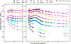 |
Fig. 1. Optical light curves of SN 2024iss. Left panel: Early-time multiband photometry within the first ten days. Right panel: Multiband light curves of SN 2024iss within the first ∼100 days. All magnitudes are corrected for the Galactic extinction. For better clarity, light curves in different bandpasses were shifted vertically by arbitrary numbers as labeled on the right. Facilities used to obtain the photometry are indicated by the legend. The last nondetection from ASAS-SN is marked by the green inverted triangle. |
Photometric observations of SN 2024iss.
2.3. Optical spectroscopy
Our spectral sequence of SN 2024iss consists of 51 spectra, spanning phases from t ≈ 1 days to 87 days after the explosion. The data set is obtained by various facilities including the Beijing Faint Object Spectrograph and Camera (BFOSC) on the Xinglong 2.16 m telescope (XLT;), the Kast double spectrograph (Miller et al. 1993) mounted on the Shane 3 m telescope at Lick Observatory, the Yunnan Faint Object Spectrograph and Camera (YFOSC) on the Lijiang 2.4 m telescope (LJT; Wang et al. 2019), the FLOYDS spectrographs (Brown et al. 2013) on the 2 m Faulkes Telescopes South and North (FTS and FTN), the Gemini Multi-Object Spectrograph (GMOS; Hook et al. 2004) on the Gemini North Telescope (GNT), the B&C spectrograph on the 1.22 m Galileo Telescope (GT), the DOLORES (Device Optimised for the LOw RESolution) on the 3.5 m Telescopio Nazionale Galileo (TNG), the Low Resolution Spectrograph 2 (LRS2; Chonis et al. 2014) mounted on the Hobby-Eberly Telescope (HET; Ramsey et al. 1998) located at McDonald Observatory, Binospec (Fabricant et al. 2019) at the MMT Observatory, the Boller and Chivens Spectrograph (B&C) on the University of Arizona’s Bok 2.3 m telescope located at Kitt Peak National Observatory, and the Multi-Object Double Spectrographs (MODS; Pogge et al. 2010) on the Large Binocular Telescope (LBT) located on Mt. Graham, Arizona USA. The observation log of optical spectroscopy is presented in Table A.3.
All spectra were processed following routines within IRAF (Tody 1986, 1993), as well as custom Python and IDL codes3, including bias subtraction, flat-field correction, and cosmic-ray removal. The FLOYDS pipeline (Valenti et al. 2014) was used to reduce the FLOYDS spectra. Spectra taken with GNT+GMOS were reduced with the Data Reduction for Astronomy from Gemini Observatory North and South (DRAGONS; Labrie et al. 2019) package. The HET spectrum were reduced by the Panacea pipeline4. Spectra taken with the Binospec on MMT were reduced using the Python-based package PypeIt (v1.17.4; Prochaska et al. 2020), while those taken with the MODS were bias and flat-field corrected using the modsCCDred package (Pogge 2019), then they were extracted and flux-calibrated with the standard IRAF routines. Wavelengths were calibrated using Fe/Ar or Fe/Ne comparison-lamp spectra taken on the same night. Flux calibration was achieved using standard stars observed at similar airmasses. We also removed the telluric features by scaling a mean telluric spectrum constructed from multiple observations of telluric standard stars to match the SN spectrum.
2.4. X-ray observations
Immediately after the explosion of SN 2024iss, rapid follow-up observations in the soft X-ray band were carried out by the Follow-up X-ray Telescope (FXT; Chen et al. 2020) on the Einstein Probe (EP) satellite (Yuan et al. 2022), the X-ray Telescope (XRT; Burrows et al. 2005) on the Swift (Gehrels et al. 2004), and the Nuclear Spectroscopic Telescope Array (NuSTAR; Harrison et al. 2013). Note that a prominent signal was detected by EP-FXT during its first epoch observations (corresponding to t ≈ +3 days after the explosion). Integration of SN 2024iss by Swift-XRT was started approximately two days after the explosion. A total of 18 observations were conducted spanning the phases from days +2 to +34. We detected prominent signals in the first two time intervals, spanning from days +1.5 to +3.7 and +4.1 to +7.1. Rebinning the Swift XRT integration to the third time interval centered at day +11 reveals a rapid decline of the X-ray luminosity. We do not detect any significant signal during the fourth time interval centered at day +35 after the explosion. Subsequent Swift observations conducted at t ≈ 207 and 277 days did not detect any signals at the location of SN 2024iss. A log of the X-ray observations is provided in Table A.1.
The FXT data were reduced with the FXT data-analysis software (fxtsoftware v1.10)5 to produce high-level science products. Swift/XRT data were processed with the online XRT product builder6 (Evans et al. 2007, 2009). NuSTAR observations were analyzed with the standard NuSTAR data-analysis software (NuSTARDAS v2.1.2) to extract science products. We fit the energy spectrum with the tbabs*apec model7. The tbabs model computes the total cross section of the gas particles along the source-Earth line of sight that induce the X-ray absorption, including the Galactic, the host, and the matter surrounding the emitting source. The apec model calculation returns the emission spectrum produced by the collisionally ionized diffuse gas. The best-fit model parameters of X-ray spectrum are tabulated in Table A.2. Due to the limited photon counts and the restricted energy coverage of FXT (0.5–10 keV), the plasma temperature (kT) of SN 2024iss at each epoch cannot be reliably constrained independently. We therefore adopted a fixed plasma temperature to the temperature estimated from the second NuSTAR observation for all other observations. The neutral hydrogen column density from the Milky Way toward the direction of SN 2024iss is 7.5 × 1019 cm−2 (Foight et al. 2016), as derived assuming it is linearly correlated with the Galactic reddening component, namely E(B-V) = 0.0084 mag.
3. Optical photometry
3.1. Photometric evolution
Figure 1 shows the UV and optical light curves of SN 2024iss. We divide the temporal evolution of the photometry into two phases, namely the early shock-cooling (from days 0 to 10 after the SN explosion) and the later radioactive decay phases. SN 2024iss was discovered very shortly after the explosion; following the serendipitous gVr-band images obtained on day 0.44, we continued the high-cadence multicolor photometric followup campaign on SN 2024iss and obtained the second epoch of observation on day 1.3. SN 2024iss reached the first V-band peak of −17.33 ± 0.26 mag on about day 2.4. This evolution is consistent with the cooling of a hot blackbody, where the peak of the emission shifts progressively to longer wavelengths as the temperature decreases.
At t ≈ 5 days after the explosion, as photons escape from the expanding shock-heated envelope, the SN luminosity becomes progressively dominated by the radioactive decay of [56]Ni, which powered the second peak of SN 2024iss. After correcting for extinction, the peak of the V-band light curve (MV = −17.43 ± 0.26 mag) was reached on day 18.7. At t ≈ 50 days after the explosion, the light curves of SN 2024iss in all observed bandpasses enter a linear decline phase, with a characteristic V-band decline rate of ∼2.0 mag (100 days)−1. As seen in other SNe IIb, SN 2024iss declines faster than the radioactive-decay rate of [56]Co → [56]Fe, 0.98 mag (100 days)−1.
Figure 2 compares the absolute V light curve of SN 2024iss with a sample of well-observed SNe IIb, including SNe 1993J (Richmond et al. 1996), 2011fu (Morales-Garoffolo et al. 2015), 2011dh (Ergon et al. 2014), 2013df (Morales-Garoffolo et al. 2014), 2016gkg (Arcavi et al. 2017; Bersten et al. 2018), and 2020acat (Medler et al. 2022). Basic observational properties of this SN sample are provided in Table 3. Considering the relatively large uncertainties in the estimation of the distance modulus among various cases, we arbitrarily shifted the light curve to match the peak of the V magnitude of SN 2024iss and aimed to compare the morphology of the light curves of different SNe IIb.
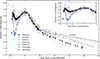 |
Fig. 2. Light curve in the V band for SN 2024iss compared to those of well-sampled cases: Type IIb SNe 1993J, 2011dh, 2013df, 2016gkg, and 2020acat. The light curves of the comparison SNe have been shifted in both magnitude and time to align with the peak magnitude and the time of the V light-curve peak of SN 2024iss. The dashed black line represents the expected decline rate of [56]Co (0.98 mag (100 day)−1; Woosley et al. 1989). The upper-right inset shows a zoom-in of the first 30 days. |
Properties of some typical Type IIb SNe compared with SN 2024iss.
SN 2024iss shows a prominent first peak, which is similar to that of SNe 1993J, 2011fu, 2013df, and 2016gkg, but distinct from that of SNe 2011dh and 2020acat. As discussed previously, SNe IIb can be further classified into two subtypes, eIIb and cIIb (Chevalier & Soderberg 2010). The prominent early peak of SN 2024iss indicates its extended-envelope nature. Among all the known cases that belong to the eIIb group, SN 2024iss is notable for its well-sampled first peak, with multiband photometry covering both the rise and the decline during the shock-cooling phase. The decline rate of the first peak in SN 2024iss is comparable to that of SN 2011fu. However, the former exhibits a shorter decline time and a shallower subsequent valley compared to those observed in SNe 1993J and 2011fu. At the [56]Ni-powered phase, as illustrated in Figure 2, the V-band light curve of SN 2024iss displays remarkable similarities to those of other comparison SNe IIb. During the linear (in mag day−1) decline phase of the light curve (from ∼60 days post-explosion), SN 2024iss exhibits a faster decline compared to that of other comparison SNe. More detailed modeling of the initial peak, the secondary peak, and the radioactive-decay tail of the light curve is presented in Sections 5, 3.4, and 7.3, respectively.
3.2. Color evolution
Figure 3 compares the extinction-corrected U − B, B − V, and g − r color curves of SN 2024iss with those of SNe 1993J, 2011fu, 2011dh, 2013df and 2016gkg. For better comparison, the V − R colors of SNe 1993J, 2011fu, 2013df, and 2016gkg were converted to g − r using the transformation relations provided by Jordi et al. (2006).
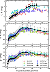 |
Fig. 3. Galactic reddening-corrected U − B, B − V, and g − r color curves of SN 2024iss compared with Galactic reddening-corrected color curves of SNe 1993J, 2011fu, 2011dh, 2013df, and 2016gkg. For display purposes, the V − R color curves of SNe 1993J, 2011fu, 2013df, and 2016gkg were converted to g − r using the transformation from Jordi et al. (2006). |
As shown in the top panel of Figure 3, the U − B color of SN 2024iss displays a continuous increase until settling to a plateau at a maximum of ∼1.2 ± 0.4 mag at t ≈ 35 days. The B − V and g − r colors of SN 2024iss exhibit similar evolution, with two distinct phases of increase of the color indices, which coincide with the first and second optical light-curve peaks. In particular, the B − V and the g − r colors of SN 2024iss increase by ∼0.35 mag and 0.67 mag within the first five days, respectively. Such an initial rise indicates a rapid decrease in photospheric temperature as fit by a blackbody function (see Sect. 3.3 and Fig. 4). From t ≈ 5 to 20 days, both the B − V and g − r colors of SN 2024iss continue to become redder, but at a much slower rate. Such a two-phase redward evolution in the early color curves is broadly consistent with the average behavior of the comparison SNe IIb shown in Figure 3. In contrast, a blueward color evolution between the two rapid increases in B − V and g − r is reported in SNe 2022crv (Dong et al. 2024) and 2024uwq (Subrayan et al. 2025).
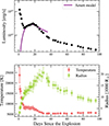 |
Fig. 4. Top: Pseudo-bolometric light curve of SN 2024iss. The purple line shows the best-fit Arnett model (Arnett 1982) to the secondary peak. Bottom: Evolution of the blackbody temperature and the photospheric radius of SN 2024iss, as indicated by the left- and right-hand ordinates, respectively. |
As the V light curve reaches its secondary peak at around day 20, the B − V and g − r colors of SN 2024iss display another redward evolution until reaching the reddest colors of ∼1.29 ± 0.37 and 0.97 ± 0.37 mag, respectively, at t ≈ 40 days. Overall, such color evolution is broadly consistent with that of other SNe IIb, with the exception of SN 2011dh, which does not show a clear initial rapid reddening phase and only exhibits a very shallow initial decline in the V band (Tsvetkov et al. 2012) and the P48 g band (Arcavi et al. 2011).
3.3. Pseudo-bolometric luminosity and temperature evolution
Using extinction-corrected photometry, we constructed the pseudobolometric light curve of SN 2024iss with the Light Curve Fitting package (Hosseinzadeh & Gomez 2020). The SED at each epoch was fit with a blackbody function, employing a Markov chain Monte Carlo routine with the emceepg package (Foreman-Mackey et al. 2013). We also included the NIR photometry published by Yamanaka et al. (2025), as the NIR contribution at later phase (a few months after the explosion) may reach up to ∼35% (Medler et al. 2022). Temporal evolutions of the constructed pseudobolometric luminosity, the blackbody temperature, and the radius of SN 2024iss are shown in Figure 4. The last two of these parameters were derived by fitting a blackbody spectrum to the SED constructed from the UV, optical, and NIR (uvw2, uvm2, uvw1, B, V, g, r, i, J, H, and K) photometry.
As shown in the top panel of Figure 4, the maximum pseudobolometric luminosity of SN 2024iss yields L = (1.2 ± 0.4)×1043erg s−1, which is observed on day 1.2. Owing to the lack of multiband photometry at even earlier phases, the constructed pseudobolometric light curve does not cover the phase before day 1.2. The pseudobolometric light curve subsequently declines until reaching a turning point on day 6.7. The light curve then rises again until a secondary peak of L = 3.1 × 1042 erg s−1, log(L/erg s−1) = 42.49 ± 0.07 is attained on day 17.6, which is coincident with the time of the V-band maximum brightness. The pseudobolometric luminosity of SN 2024iss observed at its secondary peak is slightly above the mean peak luminosity of SNe IIb given by Prentice et al. (2016), log . This may result from either a larger amount of [56]Ni synthesized during the SN explosion or a more thorough mixing of [56]Ni throughout the ejecta (Liu et al. 2025).
Both the temperature and photospheric radius of SN 2024iss show evolution similar to those of other Stripped-Envelope Supernovae (SESNe; Taddia et al. 2018). The effective temperature drops rapidly during the early phase, from ∼23 000 K to ∼8200 K within the first ∼7 days, until entering a plateau phase. It remains constant until t ≈ 18 days and then decreases, at a time roughly coincident with the V-band maximum light. The temperature evolution of SN 2024iss derived by fitting a blackbody to the SED mirrors the trend observed in the B − V and g − r color curves (see Sect. 3.2 and Fig. 3).
3.4. Estimating the [56]Ni mass
We fit the second peak of the pseudobolometric light curve with the Arnett (1982), which was first proposed as an oversimplified expanding fireball model to explain the early-time light curve of Type Ia SNe. Valenti et al. (2008) extended this model to SESNe by separating their photometric evolution into the photospheric and nebular phases, and introducing a γ-ray leakage term. This model involves two key parameters to describe the secondary peak of the bolometric light curve, namely the synthesized nickel mass in the SN ejecta (MNi), which determines the peak bolometric luminosity, and the ejecta mass (Mej), which is related to the photon diffusion time τm and the width of the bolometric light curve. According to Arnett (1982), τm can be expressed in terms of Mej and the photospheric velocity, vph:
 (1)
(1)
where β ≈ 13.8 is a constant, c denotes the speed of light and vph is the photospheric velocity. Following common assumptions for SESNe (Taddia et al. 2018; Dong et al. 2024), we adopt a constant optical opacity κopt = 0.07 cm2 g−1 and a γ−ray opacity κγ = 0.027 cm2 g−1. This model assumes all [56]Ni is placed at the center of the SN ejecta without any outward mixing, and that the opacity remains constant throughout the evolution. For a spherical SN ejecta, vph is linked to the kinetic energy and Mej through the relation
 (2)
(2)
Following the prescriptions described by Dessart & Hillier (2005), we adopt a photospheric velocity of 7500 km s−1, as measured from the absorption minimum of Fe II λ5169 in the near-maximum-light spectrum. This velocity is comparable to that of SN 1993J (8000 km s−1) and other SNe IIb (Medler et al. 2022), but is significantly lower than the velocity measured from the Hα P Cygni profile in the spectrum of SN 2024iss, which is 15000 km s−1 (Yamanaka et al. 2025).
We fit the pseudobolometric light curve of SN 2024iss spanning the phase from t ≈ +7 to +30 days with the emcee package (Foreman-Mackey et al. 2013). The time interval was chosen to encompass the secondary peak but exclude the nebular phase when the observed flux becomes dominated by various emission lines from iron-group elements. The best-fit result is shown by the purple line in the upper panel of Fig. 4, indicating MNi = 0.117 ± 0.013 M⊙, Mej = 1.27 ± 0.34 M⊙, and Ek = 0.43 ± 0.12 × 1051erg. The nickel mass derived for SN 2024iss is similar to that reported for other Type IIb SNe, such as 0.11 M⊙ for SN 2013df (Morales-Garoffolo et al. 2014). However, the ejecta mass of SN 2024iss appears to be lower than the entire SN IIb sample presented by Medler et al. (2021). Additionally, we measure the magnitude decline from maximum light to 15 days thereafter in the V-band light curve, i.e., Δm15(V) = 1.13 mag, which is larger compared to an average value of 0.93 mag derived for a sample of Type IIb SNe (Taddia et al. 2018). Such a rapid decline may not solely result from a low ejecta mass, but may also be caused by other effects such as vigorous mixing of radioactive [56]Ni throughout the SN ejecta, or by variations in the density profile of the ejecta (Liu et al. 2025). A more detailed analysis is provided in Section 7.3.
4. Optical spectroscopy
4.1. Spectral evolution
We collected a total of 51 spectra of SN 2024iss spanning the phases from t ≈ +1.3 to +87.0 days. The spectral sequences before and after t ≈ 7.0 days are shown in Figures 5 and 6, respectively. All spectra were corrected for the Galactic reddening and are presented in the rest frame. Within the first seven days after the estimated explosion, the spectra of SN 2024iss are characterized by a blue and featureless continuum. At this stage, the SN emission is dominated by the shock cooling. The outermost envelope of the exploding progenitor star manifests sufficiently high temperature at the location of the photosphere, where the high-opacity line-forming regions were not often present. We see no narrow emission features in the first few spectra of SN 2024iss, as shown in Figure 5. However, narrow emission features can be identified in the spectra of SN 1993J (Benetti et al. 1994) and 2013cu (Gal-Yam 2017) within the first days after the explosion.
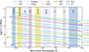 |
Fig. 5. Spectral sequence of SN 2024iss, spanning the first 7 days after the explosion. Phases are marked on the right. Different colors distinguish the different spectrographs used in the observations, as shown at the top. A log of the spectroscopy of SN 2024iss is given in Table A.3. |
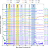 |
Fig. 6. Spectral sequence of SN 2024iss obtained during the phases from t ≈ 8 to 87 days after the explosion. The layout of the figure is similar to that of Figure 5. For the purpose of presentation, the best-fit blackbody function was subtracted from each spectrum. |
The absence of such narrow lines may indicate either a relatively low density or less radially extended CSM content around the progenitor of SN 2024iss. As the ejecta cool down, the characteristic P Cygni profiles of the Balmer lines start to emerge in the t ≈ 3.8 day spectrum. Features of He I λ5876, Hγ and Ca II λλ8498, 8542, 8662 (the NIR triplet) also can be identified in the spectra starting from t ≈ 5.3 days.
As illustrated in Figure 6, the spectral evolution of SN 2024iss after the shock-cooling phase shows a close resemblance to that of other SNe IIb (Filippenko 1997; Morales-Garoffolo et al. 2014; Medler et al. 2022). All spectra are normalized by the fit blackbody continuum. After t ≈ 18.4 days, Fe II lines develop P Cygni profiles. Meanwhile, He I λ5876, 6678 features become progressively more prominent after the shock-cooling phase. We attribute the absorption troughs at ∼4300 Å to the blending of several lines, namely He I λ4472, Mg I λ4481, and Fe II λ4549, consistent with line identifications in the literature (e.g., Hachinger et al. 2012; Silverman et al. 2009; Morales-Garoffolo et al. 2014).
Before entering the nebular phase, the Ca II λλ3943, 3969 H&K and Ca II λλ8498, 8542, 8662 NIR triplet lines are prominent blueshifted absorption features. As the ejecta cool, the [Ca II] λλ7291, 7323 doublet appears around day 32, followed by a series of oxygen lines, [O I] λλ6300, 6364 and O I λ7774. Such signatures can be clearly identified in the t ≈ 61 day spectrum. By t ≈ 87 days, as the ejecta cool, various forbidden lines and the double peak in the Ca II λλ8498, 8542, 8662 feature become even more prominent in the spectrum (see further discussion in Sect. 4.3).
4.2. Velocity evolution
The photospheric velocities of SN 2024iss as measured from Hα, Hβ, Hγ, He I λ5876, He I λ6678, Fe II λ5018, Fe II λ5169, Ca II λλ3943, 3969, and Ca II λλ8498, 8542, 8662 lines are shown in Figure 7. For each spectral feature that shows a P Cygni profile, we subtracted the pseudocontinuum and fit the residual with a Gaussian function. We then inferred the expansion velocity from the blueshifted absorption minimum. After V-band maximum brightness, velocities inferred from the Balmer lines and the He I λ5876 feature show a slower decline, which may be due to the transition of the energy source from adiabatic to radiative cooling. The Balmer lines show a similar velocity evolution, with velocities consistently higher than those of other lines. Additionally, Ca II lines also exhibit relatively high expansion velocities, possibly due to element mixing (Fransson & Chevalier 1989). At t > 25 days, measuring the Ca II velocity is difficult because of emission-dominated profiles. The Fe II λ5169 line velocities are key tracers of the receding photosphere in the expanding ejecta (Dessart & Hillier 2005). We measure a velocity of 7500 ± 500 km s−1 from the Fe II λ5169 line around the V-band peak of SN 2024iss. We also note that the P Cygni profile of the Fe II λ5169 feature suffered from increased contamination as other lines emerged, introducing larger uncertainties in profile fitting and velocity estimation. In Figure 8, we compare the velocity evolution of SN 2024iss with that of other SNe IIb.
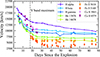 |
Fig. 7. Evolution of the expansion velocity of SN 2024iss measured from spectral features of Hα, Hβ, Hγ, He I, Fe II, and Ca II. The dashed vertical gray line marks the epoch of V light-curve peak brightness. Photospheric velocities inferred from the absorption minima of Balmer and He I λ5876 lines appear to be faster than those from other spectral features. |
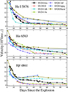 |
Fig. 8. Temporal evolution of He I λ5876, Hα, and Hβ of SN 2024iss compared to that measured for SNe 1993J, 2011dh, 2011fu, 2013df, 2016gkg, and 2020acat. |
4.3. Comparison with other Type IIb SNe
Figure 9 compares the spectra of SN 2024iss with those of SNe 1993J (Barbon et al. 1995; Matheson et al. 2000), 2011dh (Arcavi et al. 2011; Ergon et al. 2014), 2011fu (Kumar et al. 2013; Morales-Garoffolo et al. 2015; Shivvers et al. 2019), 2013df (Szalai et al. 2016; Shivvers et al. 2019), 2016gkg (Kilpatrick et al. 2017), and 2020acat (Medler et al. 2022) at similar phases. All comparison spectra were downloaded from WISEREP8 (Yaron & Gal-Yam 2012) and have been corrected for the redshifts of the host galaxies and the reported reddenings. Basic information of the comparison SNe is compiled in Table 3.
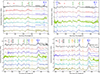 |
Fig. 9. Spectra of SN 2024iss at (a) −12, (b) 2, (c) 31, and (d) 69 days relative to V-band peak brightness compared with other well-studied SNe IIb at similar phases. Phases with respect to the V maximum are labeled. All spectra are shown in the rest frame and have been normalized. The vertical dashed lines mark the positions of certain spectral features at zero rest-frame velocity. For comparison, the gray curve underlying the spectrum of each comparison SN shows the shifted spectrum of SN 2024iss that matches their mean flux within the displayed wavelength range. |
At early phases, SNe 2024iss and 1993J exhibit similar Hα and Hβ profiles, while SN 1993J displays a more prominent He I λ5876 line. The Ca II NIR triplet profile of SN 2024iss shows a striking resemblance to that of SN 2020acat. Additionally, we note that among all the spectra of SNe IIb compared in Fig. 9 (a), SNe 2011dh and 2011fu exhibit more prominent line at ∼10 before V-band maximum brightness, indicating a prompt spectral evolution.
At around V maximum, as shown in Fig. 9 (b), both SNe 2024iss and 1993J exhibit a flat-topped emission component of Hα, which may likely be caused by the strengthening He I λ6678. In contrast, SN 2013df displays single-peaked Hα emission, while SNe 2011dh and 2011fu exhibit double-peaked profiles, likely indicating a rather prompt mixing of helium into the H-rich envelope. SN 2011fu shows the most prominent He I λ5876 feature among the sample. Additionally, SNe 2024iss and 2013df are characterized by shallower Ca II λλ8498, 8542, 8662 absorption lines relative to other comparison SNe. We also note that both SNe 2024iss and 1993J display a double-peaked feature near 4000 Å, whereas SNe 2011fu and 2016gkg show a single Ca II H&K λλ3943, 3969 emission peak. Finally, SN 2024iss shows a single-peaked line near 4800 Å which can be attributed to Hβ, where other comparison SNe display line complexes.
In Fig. 9 (c) we compare the spectrum of SN 2024iss at ∼31 days after the V-band peak to those of other comparison SNe at a similar phase. SN 2024iss exhibits broader Ca II λλ8498, 8542, 8662 absorption in comparison with other SNe. Furthermore, unlike the significantly weakened Hα absorption component observed in SNe 1993J and 2013df, such a feature still remains prominent in SNe 2024iss, 2016gkg, and 2020acat.
At t ≈ 67 days after the V-band maximum light, as shown in Fig. 9 (d), the iron features became more prominent, indicating a transition to the nebular phase, when the continuum spectral emission becomes dominated by a blend of Fe-group features. The strength of the Balmer lines is decreasing while several He I lines remain strong, highlighting the SN’s Type IIb nature. Additionally, the spectrum of SN 2024iss exhibits a double-peaked Ca II λλ8498, 8542, 8662 profile. Among the comparison sample, only SN 1993J shows a comparable feature at a similar phase. At earlier phases, these lines are blended due to line broadening. As the ejecta cool down, individual components separate and become distinguishable. The evolution of the double-peaked Ca II NIR triplet profile of SN 2024iss during the nebular phase remains an intriguing question. Additionally, similar to SNe 1993J and 2013df, SN 2024iss still shows Hα at this phase, which was no longer identified in the spectra of SN 2011fe, 2011dh, and 2020acat obtained at a similar epoch. The presence of hydrogen at this phase suggests elemental mixing or a relatively massive hydrogen envelope. Finally, we note that SN 2024iss also shows the strongest [Ca II] λλ7291, 7323 emission feature relative to the comparison SNe.
5. Shock-cooling model fitting
Among various models developed to describe the shock cooling emission, we adopt the one by Sapir & Waxman (2017, hereafter SW17) to fit the multiband light curves of SN 2024iss up to t ≈ 5 days after the explosion. The key parameters in SW17 include the envelope radius (R), the envelope mass (Menv), the shock velocity (vs, 8.5), the product of stellar mass and a numerical factor related to envelope structure (fρM), and the time of first light (t0).
SW17 assumes a polytropic density profile, where the polytropic index n = 3/2 corresponds to the case of a red supergiant with a convective envelope and n = 3 corresponds to the case of a blue supergiant with a radiative envelope. Building on the framework of Rabinak & Waxman (2011), SW17 introduced an exponential suppression factor in luminosity. This modification extends the validity of the model to a few days after the explosion. According to the different polytropic indexes (n = 3/2[3]), the bolometric luminosity is given by (following the formulation recast by Arcavi et al. 2017)
![Mathematical equation: $$ \begin{aligned} L_\mathrm{RW} = 2.0[2.1]&\times 10^{42} \nonumber \\&\times \left [ \frac{v_{s,8.5}t^{2}}{f_{\rho }M\kappa _{0.34}}\right ] ^{-0.086[-0.175]}\ \frac{v_{s,8.5}^{2}R_{13}}{\kappa _{0.34}}\ \mathrm {erg\,s}^{-1} \, , \end{aligned} $$](/articles/aa/full_html/2026/06/aa57843-25/aa57843-25-eq7.gif) (3)
(3)
![Mathematical equation: $$ \begin{aligned} L/L_\mathrm{RW} = 0.94[0.79]&\times \nonumber \\&\mathrm{exp} \left [-\left(\frac{1.67[4.57]t}{(19.5\kappa _{0.34}M_{e}v_{s,8.5}^{-1})^{0.5}}\right)^{0.8[0.73]}\right ]\, , \end{aligned} $$](/articles/aa/full_html/2026/06/aa57843-25/aa57843-25-eq8.gif) (4)
(4)
where t is the time since explosion in days, vs, 8.5 is the shock velocity in 108.5 cm s−1, R13 is the envelope radius in 1013 cm, κ0.34 is the opacity in 0.34 cm2 g−1, and M is the ejecta mass (core mass Mc + envelope mass Me) in solar masses. When Rc/R ≪ 1, fρ can be approximated as
 (5)
(5)
The temporal evolution of the color temperature is given as
![Mathematical equation: $$ \begin{aligned} T = 2.05[1.96]&\times 10^{4} \nonumber \\&\,\,\times \left [\frac{v_{s,8.5}^{2}t^{2}}{f_{\rho }M\kappa _{0.34}}\right ]^{0.027[0.016]}\left(\frac{R_{13}}{\kappa _{0.34}}\right)^{0.25} t^{-0.5}\, \mathrm{K}\, . \end{aligned} $$](/articles/aa/full_html/2026/06/aa57843-25/aa57843-25-eq10.gif) (6)
(6)
Assuming that the continuum emission of SN 2024iss can be well approximated by a blackbody spectrum, we can calculate the photospheric radius from the Stefan-Boltzmann law and fit the model to the multiband photometry. We fit the Swift UVOT uvw2, uvm2, uvw1, B, V, g, r, and i-band light curves of SN 2024iss with the open-source package Light Curve Fitting (Hosseinzadeh & Gomez 2020), implementing the analytic expression given by SW17, with an index n = 3/2. We restrict the fit to data obtained within five days after the estimated time of explosion, as beyond this point the energy input from the radioactive decay of [56]Ni exceeds 30% (see Sect. 3.4) and therefore biases the results. Within five days after explosion, the blackbody temperature satisfies the criterion T > 0.7 eV, ensuring the validity of the SW17 model during the period. The fit was performed using a Markov chain Monte Carlo routine with 30 walkers and 2000 steps (1000 steps for burn-in). The additional scatter term (σ) was included to account for intrinsic variability and deviations from the blackbody assumption.
The Markov chain Monte Carlo parameters distributions and the best-fit model multiband light curves are presented in Figure 10. The parameters that best describe the shock-cooling phase as follows: R = 244 ± 43 R⊙, Menv = 0.11 ± 0.04 M⊙, vs, 8.5 = (1.9 ± 0.3)×108.5 cm s−1, fρM = 100 ± 65 M⊙ and texp = 60442.41 ± 0.05 d. The model light curves agree fairly well with the observations. The inferred envelope mass and radius of SN 2024iss are larger than those of SN 2016gkg (∼0.03 M⊙, ∼141 R⊙; Piro et al. 2021), indicating a more extended envelope than in Type cIIb SNe. The envelope mass of SN 2024iss is lower than that of SN 1993J (∼0.2 M⊙; Woosley et al. 1994), suggesting that its envelope is less extended than that of some Type eIIb SNe.
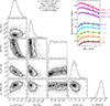 |
Fig. 10. Corner plot presenting the posterior distributions of the SW17 shock-cooling light-curve model of SN 2024iss. The fit to the early light curves was restricted to five days after the estimated time of the SN explosion. The best-fit parameters are listed at the top of the figure. The upper-right inset presents the model light curves that best fit the multiband photometry, as displayed by color coded curves and symbols, respectively. |
6. X-ray constraints on the circumstellar medium
Figure 11 shows the unabsorbed 3–10 keV X-ray luminosity of SN 2024iss. The errors were estimated by adding the uncertainties in the X-ray photometry and the distance modulus in quadrature. As the temperature of post-shock gas is higher than 2 × 10⁷ K, thermal bremsstrahlung emission in the forward shock dominates over the cooling (Fransson et al. 1996; Chevalier & Fransson 2017). Assuming a homogeneous wind with vwind = 10 km s−1 according to Fransson et al. (1996), our best-fit result is consistent with a mass-loss rate of Ṁ = 1.6 × 10⁻⁵ M⊙ yr−1 and a shock velocity of  9.5 × 108 cm s−1. Based on the 3σ and 5σ confidence intervals of the 3–10 keV luminosity as indicated by the green and purple shaded regions in Fig. 11, the mass-loss rate is constrained as (1.2–1.9) ×10−5 and (1.0–2.2) × 10−5 M⊙ yr−1, respectively. The mass-loss rate inferred for the X-ray observations of SN 2024iss is comparable to those of SNe 1993J (4 × 10⁻⁵ M⊙ yr−1; Fransson et al. 1996) and 2013df (i.e., 8 × 10⁻⁵ M⊙ yr−1, Kamble et al. 2016). The shock velocity inferred from the X-ray light curve of SN 2024iss is consistent with that estimated by the shock-cooling model as discussed in Section 5, vs = (6.0 ± 0.9)×108 cm s−1, but is much smaller than the result inferred from the early-time Hα velocity (vHα = 1.94 × 109cm s−1).
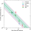 |
Fig. 11. Unabsorbed X-ray luminosity of SN 2024iss observed in the 3–10 keV band. The red, green, and blue data points represent the observations conducted with NuSTAR, Swift-XRT, and EP-FXT, respectively. The black line shows the best-fit thermal bremsstrahlung model, with a mass-loss rate of 1.6 × 10⁻⁵ M⊙ yr−1 and a shock velocity of 9.5 × 108 cm s−1. The green and purple shaded areas indicate the 3σ and 5σ confidence regions, respectively. |
To further investigate the CSM properties, we also used the method of emission measure (EM) to constrain the density structure of the CSM:
 (7)
(7)
where ρ(r) represents the mass density of the CSM at radius r, VCSM ≈ 4 πr2Δr is the volume of the shocked CSM shell, with Δr ≈ 0.1r denoting the thickness of the forward-shocked CSM. We adopted a mean molecular weight of μ = 0.61 for the ionized CSM with solar metallicity, where μe ≈ 1.3 and μH ≈ 1.15. The EM parameter can be derived from the “Norm” column in Table A.2.
Figure 12 shows the radial density profile of the CSM around SN 2024iss (ρCSM) as inferred from the EM method, together with that of the homogeneous wind with different mass-loss rates. The CSM density lies between the 10−5 and 10−4 M⊙ yr−1 curves of steady mass loss, with a mean value of (5.55 ± 1.57) × 10−5 M⊙ yr−1. This estimate is higher than the value derived from the X-ray light curve of SN 2024iss. However, it is comparable to the mass loss rate of 8 × 10⁻⁵ M⊙ yr−1 estimated for SN 2013df, assuming a wind velocity of 10 km s−1 (Kamble et al. 2016). The discrepancy may be due to the unusually low intrinsic neutral hydrogen column density of SN 2024iss, namely NH < 8 × 1019 cm−2 (84% confidence level) after subtracting the Galactic contribution. The low column density would introduce a degeneracy in the X-ray spectral fitting and thus overestimate the mass-loss rate compared to the free-free emission model. A power-law fit to this profile yields ρCSM ∝ R−2.19±0.10, which is consistent (within ∼2σ) with the canonical R−2 expected for a steady wind.
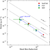 |
Fig. 12. Circumstellar material density profile as inferred from the EM. Data from NuSTAR, Swift-XRT, and EP-FXT are indicated by the red, green, and blue circles, respectively. The dashed gray lines represent the wind-like density profiles corresponding to mass-loss rates of Ṁ = 10−5, 10−4, 10−3 M⊙ yr−1. The dashed blue line denotes the power-law fit to the X-ray light curve. The inferred radial density profile ρCSM ∝ R−2.19 ± 0.10 is compatible with a homogeneous mass-loss wind within ∼2σ. |
In Figure 13, we compare the 0.3–10 keV X-ray luminosity evolution of SN 2024iss with that of several other Type IIb SNe, including SNe 1993J (Chandra et al. 2009), 2011dh (Soderberg et al. 2012), 2013df (Kamble et al. 2016), 2016gkg (Dwarkadas 2025), and 2024abfo (Reguitti et al. 2025). The X-ray luminosity of SNe 1993J and 2013df were estimated in the 0.3–8 keV band. The uncertainty introduced from different bands can be neglected, as the X-ray emission contributes little above 8 keV. Among the comparison sample, SN 1993J is found to follow a power-law decline with an index of ∼ − 0.68 (see the black dashed line in Fig. 13). SN 2024iss, SN 1993J, and SN 2016gkg exhibit an overall higher X-ray luminosity in comparison with SN 2011dh and SN 2024abfo.
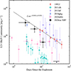 |
Fig. 13. X-ray luminosity evolution at 0.3–10 keV of SN 2024iss compared with that of SNe 1993J (Chandra et al. 2009), 2011dh (Soderberg et al. 2012), 2013df (Kamble et al. 2016), 2016gkg (Dwarkadas 2025), and 2024abfo (Reguitti et al. 2025). While most of the comparison data are in the 0.3–10 keV band, the fluxes of SNe 1993J and 2013df were measured in the 0.3–8 keV band. |
The high X-ray luminosity of the first three events above can be attributed to an extended hydrogen-rich envelope and dense wind-like CSM (Kamble et al. 2016). In contrast, those Type IIb SNe that are faint in the X-ray band may arise from more compact progenitors with a weaker ejecta-CSM interaction. Following the framework of Chevalier & Soderberg (2010), we classify SN 2024iss as Type eIIb, which is compatible with its double-peaked optical light curve and high mass-loss rate, as observed in SNe 1993J, 2013df, and 2011hs.
7. Discussion
7.1. The progenitor of SN 2024iss
The best fit to the Arnett model based on the second light-curve peak of SN 2024iss suggests an ejecta mass of Mej = 1.27 ± 0.34 M⊙ (see Section 3.4). Assuming a typical mass for the neutron star remnant of 1.4 M⊙ (Thorsett & Chakrabarty 1999), we estimate a helium core mass of Mremnant + Mej + Menv = 2.8 M⊙. Using the progenitor grid of Sukhbold et al. (2016), this indicates a zero-age main-sequence (ZAMS) mass of MZAMS = 9–11 M⊙, similar to that inferred for SN 2016gkg (Kilpatrick et al. 2022) and compatible with the predicted mass range of SN IIb progenitors in a binary system (Yoon et al. 2017). By fitting the first peak in the optical light curves with the shock-cooling model presented by P21, we infer that the mass and radius of the H envelope of SN 2024iss are Menv = 0.11 ± 0.04 M⊙ and Renv = 224 ± 43 R⊙ (see Sect. 5). The inferred mass and radius favors for a yellow supergiant progenitor star. In contrast, models involving single Wolf-Rayet stars are not able to produce an ejecta mass lower than 5 M⊙ (Lyman et al. 2016). A binary system may naturally account for the partially depleted H envelope required for the progenitor of SN 2024iss.
7.2. SN 2024iss: Bridging the gap between Types eIIb and cIIb
Note that in the classification scheme of Yoon et al. (2017), the envelope mass of SN 2024iss is close to the threshold of 0.15 M⊙ adopted to distinguish between Types eIIb and cIIb. For comparison, the compact Type IIb SN 2016gkg has an envelope mass of ∼0.03 M⊙ (Piro et al. 2021), while the extended Type IIb SN 1993J exhibits a much larger envelope mass of ∼0.2 M⊙ (Woosley et al. 1994). Similarly, the envelope radius of SN 2024iss is larger than that of the compact SN 2008ax (∼40 R⊙; Folatelli et al. 2015), but smaller than that of SN 1993J (∼575 R⊙; Woosley et al. 1994). Moreover, SN 2024iss and other Type eIIb SNe, such as SNe 1993J and 2011fu, exhibit a shallower valley than Type cIIb SNe, similar to SNe 2016gkg and 2011dh in Fig. 2. Additionally, as illustrated in Fig. 13, the X-ray luminosity of SN 2024iss is overall higher than that of Type IIb SNe with a less extended envelope, such as SNe 2011dh and 2016gkg, but lower than that of SN 1993J, whose progenitor had a more massive and extended H envelope. Taken together, the envelope properties and X-ray emission suggest that SN 2024iss likely represents a transitional object lying between the compact and extended subtypes of Type IIb SNe.
To investigate the properties of SN 2024iss and the CSM-envelope connection further, following Maeda et al. (2015), we plot in Figure 14 the mass-loss rate per unit wind velocity (Ṁ/vw) against the envelope radius. The choice of the former parameter minimizes the uncertainties due to the assumption of wind velocities. The mass-loss rates are estimated from the X-ray analyses of SNe 1993J (Fransson et al. 1996), 2008ax (Roming et al. 2009), 2011dh (Maeda et al. 2014), and 2013df (Kamble et al. 2016). The mass-loss rate of SN 2013df was adopted from Bufano et al. (2014), based on an analysis of its radio light curves. The progenitor radius was inferred through a comparison between the SED yielded from archival preexplosion images obtained by the Hubble Space Telescope and stellar-evolution tracks: SNe 1993J (Maund et al. 2004), 2011dh (Maund et al. 2011), 2013df (Van Dyk et al. 2014), and 2008ax (Folatelli et al. 2015). The progenitor radius of SN 2011hs was inferred by modeling its bolometric light curve (Bufano et al. 2014). We adopt the progenitor radii of Type Ib/c SNe from Maeda et al. (2012). The mass-loss rates of Type Ib/c SNe were inferred from their radio light curves, assuming a typical wind velocity of ∼1000 km s−1 (Chevalier & Fransson 2006).
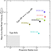 |
Fig. 14. Comparison between the mass-loss rate normalized by wind velocity (Ṁ/vw) and the progenitor radius. The shaded region indicates typical CSM densities of Type Ib/c SNe (Chevalier & Fransson 2006), though these estimates may suffer from systematic uncertainties of up to an order of magnitude (Maeda et al. 2012). Color coded symbols represent the estimated values for different SNe as labeled. The upper-right to lower-left arrow illustrates a possible evolutionary sequence from Type eIIb to cIIb and eventually to Type Ib/Ic SNe. |
As shown in Fig. 14, SN 2024iss lies in between the eIIb and cIIb groups. This supports the empirical relation proposed by Maeda et al. (2015), where more extended progenitors tend to have experienced a stronger mass loss. Furthermore, there exists a transitional subtype between SNe IIL and SNe IIb, the Type II short-plateau SNe. These events show plateaus lasting only several tens of days, and are characterized by relatively massive H envelopes (∼1.7 M⊙) and high mass-loss rates of ∼ 10−2 M⊙ yr−1, as inferred for the sample presented by Hiramatsu et al. (2021). Also, Farah et al. (2025a) classified transitional SNe IIb lying between Type II short-plateau SNe and normal Type IIb SNe, with envelope masses of around 0.6–0.8 M⊙. We expect Type II short-plateau SNe and these transitional Type IIb SNe to emerge in the upper-right region of Fig. 14, offering further insights into the relationship between CSM and envelope in H-rich SNe.
7.3. Implications of the low ejecta mass of SN 2024iss
The Arnett model fit to the pseudobolometric light curve of SN 2024iss suggests an ejecta mass of 1.27 ± 0.34 M⊙ and a [56]Ni mass of 0.117 ± 0.013 M⊙. While the latter mass value is consistent with the average value derived for SNe IIb, the ejecta mass of SN 2024iss is lower than that of all Type IIb SNe compiled by Rodríguez et al. (2023). The faint and fast Type IIb SN 2011hs exhibits a similar ejecta mass and explosion energy compared to that of SN 2024iss, but with a significantly lower [56]Ni mass (Bufano et al. 2014).
The secondary peak of SN 2024iss reached MV = −17.43 ± 0.26 mag, consistent with the average of −17.4 mag from the sample of (Taddia et al. 2018). However, it appears to be a faster decliner as indicated by its Δm15(V) = 1.13 mag (see Sect. 3.4), compared to the mean value of 0.93 mag for SNe IIb (Taddia et al. 2018) and 0.88 mag for SNe IIb (Rodríguez et al. 2023). The late-time decay rate also approaches 2 mag (100 days)−1, one of the steepest in the sample. This is consistent with the trend reported by Taddia et al. (2018), where objects with larger Δm15(V) also exhibit a steeper late-time decline. Taddia et al. (2018) explained this trend by noting that objects with higher Ek/Mej ratios are less efficient in trapping γ-rays and therefore exhibit a steeper late-time decline and a narrower light-curve peak.
Prentice et al. (2019) found that the ejecta masses of SNe IIb exhibited a bimodal distribution peaking at 1.9 and 3.9 M⊙, as represented by SNe 1993J (Mej ≈ 2.2 M⊙, Lyman et al. 2016) and 2016gkg (Mej ≈ 3.4 M⊙, Bersten et al. 2018), respectively. Such a bimodal mass distribution of the ejecta may indicate a discontinuity of the intrinsic properties of Type IIb SNe with one group having more extended and the other having a rather compact envelope. The ejecta mass of SN 2024iss falls within the lower ejecta mass regime, consistent with its Type eIIb classification.
Ayala et al. (2025) also found that although the inferred [56]Ni masses of Type eIIb and cIIb SNe are similar. However, the former group tends to have a lower average ejecta mass. Das et al. (2023) studied a sample of Ca-rich SNe IIb, which exhibit low ejecta masses and are inferred to originate from progenitors with MZAMS < 12 M⊙. They suggest that progenitors with smaller initial masses may develop larger envelope radii. According to Dewi et al. (2002) and Dewi & Pols (2003), a progenitor star with such an extended envelope may expand sufficiently to fill its Roche lobes again and undergo additional episodes of mass transfer. This process can further strip the envelope and enrich the CSM and is thus compatible with the low ejecta mass observed in SN 2024iss.
Taken together, these results indicate that Type eIIb and cIIb SNe may arise from progenitors with similar initial ZAMS masses but diverging in their final envelope and ejecta properties. Moreover, the progenitor ZAMS mass of Type Ib SN iPTF13bvn is constrained to be 10–12 M⊙ (Eldridge et al. 2023), similar to the ZAMS mass of SN 2024iss as indicated in Section 7.1. The interaction with the companion star may provide a natural explanation for the differences between Type Ib, cIIb, and eIIb SNe. In particular, an enhanced CSM enrichment during the common-envelope phase may take place before the SN explosion. Maeda et al. (2022) emphasized that instead of the initial mass of the exploding star, the binary separation and the orbital period may play a more critical role in determining the observational properties of the SN explosion.
It is important to note, however, that the Arnett model assumes a constant opacity and fixed photospheric velocity, which may introduce systematic uncertainties in the derived parameters. For instance, adopting a photospheric velocity of 15 000 km s−1 following Yamanaka et al. (2025), the Arnett model yields a larger ejecta mass of Mej = 2.64 ± 0.53 M⊙, but the corresponding kinetic energy (Ek = (3.54 ± 0.83)×1051erg) would be unrealistically high for a Type IIb SN. Alternatively, if we adopt an opacity of κ = 0.2 cm2 g−1 as suggested by Nagy & Vinkó (2016) and maintain the same photospheric velocity of 15000 km s−1, the fit yields Mej = 1.23 ± 0.23 M⊙ and Ek = (1.64 ± 0.3)×1051erg. Taken together, these estimates imply an ejecta mass in the range of 1.23–2.64 M⊙. However, considering the steep decline of the radioactive tail, a lower ejecta mass appears more plausible for SN 2024iss. With additional data obtained during the nebular phase, it should be possible to better constrain the ejecta mass following Wheeler et al. (2015) and Haynie & Piro (2023).
8. Conclusions
We have presented optical, UV, and X-ray observations of SN 2024iss, a Type IIb SN with a prominent double peak in optical bands and bright thermal X-ray emission. We summarize our key findings as follows.
(1) The optical light curves of SN 2024iss exhibit a double-peak feature. The first V-band peak, which can be attributed to shock cooling, occurred ∼2.4 days after the explosion and reached a peak magnitude of MV = −17.33 ± 0.26. The second peak, powered by [56]Ni decay, reached a peak magnitude of MV = −17.43 ± 0.26 at ∼18.7 days after the SN explosion. The photometric follow-up campaign on SN 2024iss was carried out starting from ∼0.87 days after the last nondetection, which corresponds to ∼0.44 days after the SN explosion. The prompt observations make SN 2024iss one of the most well-sampled SNe IIb during the early phases.
(2) We measure the photospheric velocity of SN 2024iss to be ∼19 400 km s−1 from the absorption minimum of the P Cygni profile of Hα in the earliest spectrum obtained at day 3.82. The velocity decreased to ∼13 600 km s−1 after the secondary peak of the V-band light curve. The Hα and Hβ features remain detectable in our last spectrum obtained at t ≈ 87 days after the SN explosion, indicating the presence of a hydrogen-rich ejecta, which is similar to that observed in SN 1993J (Filippenko et al. 1994).
(3) We fit the second peak of the pseudobolometric light curve of SN 2024iss with an Arnett-like model and adopted a photospheric velocity of 7500 km s−1 based on the Fe II λ5169 line measured around the V-band maximum brightness. The best-fitting parameters are MNi = 0.117 ± 0.013 M⊙, Mej = 1.27 ± 0.34 M⊙, and Ek = (0.43 ± 0.12)×1051erg. The inferred [56]Ni mass is typical for Type IIb SNe, while the relatively low ejecta mass is compatible with the rapid decline in luminosity, as indicated by the large Δm15(V) value of 1.13 mag, compared to an average of 0.93 mag for Type IIb SNe (Taddia et al. 2018).
(4) We fit the multiband shock-cooling peak of SN 2024iss using the P21 model, which provides a plausible description of the data. The best-fit parameters are Renv = 244 ± 43 R⊙, Menv = 0.11 ± 0.04 M⊙, and vs = (1.67 ± 0.07)×104 km s−1.
(5) SN 2024iss exhibits bright thermal bremsstrahlung emission from the forward shock. The strength of the emission is comparable to that observed in SNe 1993J and 2013df. Assuming a wind velocity of 10 km s−1, the best fit to the X-ray light curve of SN 2024iss indicates a mass-loss rate of Ṁ = 1.6 × 10⁻⁵ M⊙ yr−1 and a shock velocity of 9.5 × 108 cm s−1. An independent estimate based on the EM gives a slightly higher mass-loss rate of (5.55 ± 1.57) × 10−5 M⊙ yr−1.
The combination of the optical and X-ray observations provides a powerful approach to probe the physical properties of SESNe. In particular, the prompt X-ray emissions from SNe obtained within the first hours after the explosion, as facilitated by wide-field sky surveys such as EP (Yuan et al. 2022), will enable systematic characterization of their immediate environment and shed light on the mass-loss process and explosion mechanisms of SESNe.
Data availability
The full Table 2 is available at the CDS via https://cdsarc.cds.unistra.fr/viz-bin/cat/J/A+A/710/A33. The spectroscopic data presented here can be retrieved from WISeREP (Yaron & Gal-Yam 2012).
Acknowledgments
We thank Yi Yang for helpful suggestions on the writing and for valuable discussions. This work is supported by the National Science Foundation of China (NSFC grants 12288102 and 12033003), the Tencent Xplorer Prize, and the Ma Huateng Foundation. The LCO group is supported by U.S. National Science Foundation (NSF) grants AST-1911151 and AST-2308113. Jujia Zhang is supported by the National Key Research and Development Program of China (NKRDPC) with grant 2021YFA1600404, the NSFC(grants 12173082, 12333008, and 12225304), the Yunnan Fundamental Research Projects (YFRP; grants 202501AV070012, 202401BC070007, 202201AT070069, and 202501AS070005), the Top-notch Young Talents Program of Yunnan Province, the Light of West China Program provided by the Chinese Academy of Sciences (CAS), and the International Centre of Supernovae, Yunnan Key Laboratory (grant 202302AN360001). WXL is supported by NSFC (12120101003 and 12373010), the National Key R&D Program (2022YFA1602902 and 2023YFA1607804), and Strategic Priority Research Program of CAS (XDB0550100 and XDB0550000). DFX is supported by the NSFC(grant 12503047). Time-domain research by the University of Arizona team and D.J.S. is supported by NSF grants AST-2108032, AST-2308181, AST-2407566, and AST-2432036, and the Heising-Simons Foundation under grant 2020-1864. A.P., A.R., and G.V. acknowledge support from the PRIN-INAF 2022 project “Shedding light on the nature of gap transients: from the observations to the model.” A.R. also acknowledges financial support from the GRAWITA Large Program Grant (PI P. D’Avanzo). Y.-Z. Cai is supported by NSFC (grant 12303054), the NKRDPC (grant 2024YFA1611603), the YFRP (grants 202401AU070063, 202501AS070078), and the International Centre of Supernovae, Yunnan Key Laboratory (grant 202302AN360001). J.V. is supported by the NKFIH-OTKA Grant K142534. Maokai Hu is funded by China Postdoctoral Science Foundation (Certificate Number 2025T180872). This work is sponsored by the Natural Science Foundation of Xinjiang Uygur Autonomous Region under grant 2024D01D32, Tianshan Talent Training Program grants 2023TSYCLJ0053 and 2023TSYCCX0101, the Central Guidance for Local Science and Technology Development Fund under grant ZYYD2025QY27, and the NSFC (grants 12433007, 12373038). A.V.F.’s research group at UC Berkeley acknowledges financial assistance from the Christopher R. Redlich Fund, as well as donations from Gary and Cynthia Bengier, Clark and Sharon Winslow, Alan Eustace and Kathy Kwan, William Draper, Timothy and Melissa Draper, Briggs and Kathleen Wood, Sanford Robertson (W.Z. is a Bengier-Winslow-Eustace Specialist in Astronomy, T.G.B. is a Draper-Wood-Robertson Specialist in Astronomy), and numerous other donors. This work was partly supported by the Urumqi Nanshan Astronomy and Deep Space Exploration Observation and Research Station of Xinjiang (XJYWZ2303). This study uses observations obtained with the Hobby-Eberly Telescope, which is a joint project of the University of Texas at Austin, the Pennsylvania State University, Ludwig-Maximilians-Universität München, and Georg-August-Universität Göttingen. The HET is named in honor of its principal benefactors, William P. Hobby and Robert E. Eberly. The Low Resolution Spectrograph 2 (LRS2) was developed and funded by the University of Texas at Austin McDonald Observatory and Department of Astronomy and by Pennsylvania State University. We thank the Leibniz-Institut für Astrophysik Potsdam (AIP) and the Institut für Astrophysik Göttingen (IAG) for their contributions to the construction of the integral field units. Based in part on observations obtained as part of (GN-2024A-Q-403; P.I. Jennifer Andrews) at the international Gemini Observatory, a program of the U.S. NSF NOIRLab, which is managed by the Association of Universities for Research in Astronomy (AURA) under a cooperative agreement with the U.S. NSF on behalf of the Gemini Observatory partnership: the NSF (United States), National Research Council (Canada), Agencia Nacional de Investigación y Desarrollo (Chile), Ministerio de Ciencia, Tecnología e Innovación (Argentina), Ministério da Ciência, Tecnologia, Inovações e Comunicações (Brazil), and Korea Astronomy and Space Science Institute (Republic of Korea). These observations were processed using DRAGONS (Data Reduction for Astronomy from Gemini Observatory North and South). This work was enabled by observations made from the Gemini North telescope, located within the Maunakea Science Reserve and adjacent to the summit of Maunakea. We are grateful for the privilege of observing the Universe from a place that is unique in both its astronomical quality and its cultural significance. Based in part on observations collected at the Copernico and Schmidt telescopes (Asiago Mount Ekar, Italy) of the INAF – Osservatorio Astronomico di Padova, and at the Galileo telescope (Asiago Pennar, Italy) of the Physics and Astronomy Department of Padova University. The LBT is an international collaboration among institutions in the United States, Italy, and Germany. LBT Corporation Members are The University of Arizona on behalf of the Arizona Board of Regents; Istituto Nazionale di Astrofisica, Italy; LBT Beteiligungsgesellschaft, Germany, representing the Max-Planck Society, The Leibniz Institute for Astrophysics Potsdam, and Heidelberg University; The Ohio State University, and The Research Corporation, on behalf of The University of Notre Dame, University of Minnesota, and University of Virginia. A major upgrade of the Kast spectrograph on the Shane 3 m telescope at Lick Observatory, led by Brad Holden, was made possible through generous gifts from the Heising-Simons Foundation, William and Marina Kast, and the University of California Observatories. Research at Lick Observatory is partially supported by a generous gift from Google. This paper made use of the modsCCDRed data-reduction code developed in part with funds provided by NSF grants AST-9987045 and AST-1108693. Some observations reported here were obtained at the MMT Observatory, a joint facility of the University of Arizona and the Smithsonian Institution. We acknowledge the observational data taken with the Einstein Probe (EP), a space mission supported by the Strategic Priority Program on Space Science of the Chinese Academy of Sciences, in collaboration with ESA, MPE, and CNES (grant XDA15310000), the Strategic Priority Research Program of the Chinese Academy of Sciences (grant XDB0550200) and the NKRDPC (grant 2022YFF0711500). We also acknowledge the observational data taken with Swift and NuSTAR. A. V. Filippenko is grateful for the hospitality of the Hagler Institute for Advanced Study as well as the Department of Physics and Astronomy at Texas A&M University during part of this investigation.
References
- Arcavi, I., Gal-Yam, A., Yaron, O., et al. 2011, ApJ, 742, L18 [Google Scholar]
- Arcavi, I., Hosseinzadeh, G., Brown, P. J., et al. 2017, ApJ, 837, L2 [NASA ADS] [CrossRef] [Google Scholar]
- Arnett, W. D. 1982, ApJ, 253, 785 [Google Scholar]
- Ayala, B., Anderson, J. P., Pignata, G., et al. 2025, A&A, 701, A128 [NASA ADS] [CrossRef] [EDP Sciences] [Google Scholar]
- Bai, C.-H., Feng, G.-J., Zhang, X., et al. 2020, Res. Astron. Astrophys., 20, 211 [Google Scholar]
- Barbieri, C., Bhatia, R. K., Bonoli, C., et al. 1994, SPIE, 2199, 10 [Google Scholar]
- Barbon, R., Benetti, S., Cappellaro, E., et al. 1995, A&AS, 110, 513 [NASA ADS] [Google Scholar]
- Bellm, E. C., Kulkarni, S. R., Graham, M. J., et al. 2019, PASP, 131, 018002 [Google Scholar]
- Benetti, S., Patat, F., Turatto, M., et al. 1994, A&A, 285, L13 [NASA ADS] [Google Scholar]
- Bersten, M. C., Folatelli, G., García, F., et al. 2018, Nature, 554, 497 [Google Scholar]
- Breeveld, A. A., Landsman, W., Holland, S. T., et al. 2011, Am. Inst. Phys. Conf. Ser., 1358, 373 [NASA ADS] [Google Scholar]
- Brennan, S. J., & Fraser, M. 2022, A&A, 667, A62 [NASA ADS] [CrossRef] [EDP Sciences] [Google Scholar]
- Brown, T. M., Baliber, N., Bianco, F. B., et al. 2013, PASP, 125, 1031 [Google Scholar]
- Bufano, F., Pignata, G., Bersten, M., et al. 2014, MNRAS, 439, 1807 [Google Scholar]
- Burrows, D. N., Hill, J. E., Nousek, J. A., et al. 2005, Space Sci. Rev., 120, 165 [Google Scholar]
- Cardelli, J. A., Clayton, G. C., & Mathis, J. S. 1989, ApJ, 345, 245 [Google Scholar]
- Chandra, P., Dwarkadas, V. V., Ray, A., Immler, S., & Pooley, D. 2009, ApJ, 699, 388 [CrossRef] [Google Scholar]
- Chen, Y., Cui, W., Han, D., et al. 2020, SPIE Conf. Ser., 11444, 114445B [Google Scholar]
- Chevalier, R. A., & Fransson, C. 2006, ApJ, 651, 381 [NASA ADS] [CrossRef] [Google Scholar]
- Chevalier, R. A., & Fransson, C. 2017, Thermal and Non-thermal Emission from Circumstellar Interaction (Springer International Publishing), 875 [Google Scholar]
- Chevalier, R. A., & Soderberg, A. M. 2010, ApJ, 711, L40 [NASA ADS] [CrossRef] [Google Scholar]
- Chonis, T. S., Hill, G. J., Lee, H., Tuttle, S. E., & Vattiat, B. L. 2014, SPIE, 9147, 91470A [Google Scholar]
- Das, K. K., Kasliwal, M. M., Fremling, C., et al. 2023, ApJ, 959, 12 [CrossRef] [Google Scholar]
- Dessart, L., & Hillier, D. J. 2005, A&A, 439, 671 [NASA ADS] [CrossRef] [EDP Sciences] [Google Scholar]
- Dessart, L., Gutiérrez, C. P., Ercolino, A., Jin, H., & Langer, N. 2024, A&A, 685, A169 [NASA ADS] [CrossRef] [EDP Sciences] [Google Scholar]
- Dewi, J. D. M., & Pols, O. R. 2003, MNRAS, 344, 629 [NASA ADS] [CrossRef] [Google Scholar]
- Dewi, J. D. M., Pols, O. R., Savonije, G. J., & van den Heuvel, E. P. J. 2002, MNRAS, 331, 1027 [CrossRef] [Google Scholar]
- Dong, Y., Valenti, S., Ashall, C., et al. 2024, ApJ, 974, 316 [NASA ADS] [CrossRef] [Google Scholar]
- Dwarkadas, V. V. 2025, Universe, 11, 161 [Google Scholar]
- Eldridge, J. J., & Maund, J. R. 2016, MNRAS, 461, L117 [NASA ADS] [CrossRef] [Google Scholar]
- Ergon, M., Sollerman, J., Fraser, M., et al. 2014, A&A, 562, A17 [NASA ADS] [CrossRef] [EDP Sciences] [Google Scholar]
- Evans, P. A., Beardmore, A. P., Page, K. L., et al. 2007, A&A, 469, 379 [NASA ADS] [CrossRef] [EDP Sciences] [Google Scholar]
- Evans, P. A., Beardmore, A. P., Page, K. L., et al. 2009, MNRAS, 397, 1177 [Google Scholar]
- Fabricant, D., Fata, R., Epps, H., et al. 2019, PASP, 131, 075004 [NASA ADS] [CrossRef] [Google Scholar]
- Fan, Y.-F., Bai, J.-M., Zhang, J.-J., et al. 2015, Res. Astron. Astrophys., 15, 918 [Google Scholar]
- Farah, J. R., Howell, D. A., Hiramatsu, D., et al. 2025a, arXiv e-prints [arXiv:2509.12470] [Google Scholar]
- Farah, J. R., Howell, D. A., Terreran, G., et al. 2025b, ApJ, 984, 60 [Google Scholar]
- Filippenko, A. V. 1997, ARA&A, 35, 309 [NASA ADS] [CrossRef] [Google Scholar]
- Filippenko, A. V., Matheson, T., & Ho, L. C. 1993, ApJ, 415, L103 [NASA ADS] [CrossRef] [Google Scholar]
- Filippenko, A. V., Matheson, T., & Barth, A. J. 1994, AJ, 108, 2220 [NASA ADS] [CrossRef] [Google Scholar]
- Fixsen, D. J., Cheng, E. S., Gales, J. M., et al. 1996, ApJ, 473, 576 [Google Scholar]
- Foight, D. R., Güver, T., Özel, F., & Slane, P. O. 2016, ApJ, 826, 66 [Google Scholar]
- Folatelli, G., Bersten, M. C., Kuncarayakti, H., et al. 2015, ApJ, 811, 147 [Google Scholar]
- Foreman-Mackey, D., Hogg, D. W., Lang, D., & Goodman, J. 2013, PASP, 125, 306 [Google Scholar]
- Fransson, C., & Chevalier, R. A. 1989, ApJ, 343, 323 [NASA ADS] [CrossRef] [Google Scholar]
- Fransson, C., Lundqvist, P., & Chevalier, R. A. 1996, ApJ, 461, 993 [NASA ADS] [CrossRef] [Google Scholar]
- Fukugita, M., Ichikawa, T., Gunn, J. E., et al. 1996, AJ, 111, 1748 [Google Scholar]
- Gal-Yam, A. 2017, Observational and Physical Classification of Supernovae (Springer International Publishing), 195 [Google Scholar]
- Gehrels, N., Chincarini, G., Giommi, P., et al. 2004, ApJ, 611, 1005 [Google Scholar]
- Georgy, C. 2012, A&A, 538, L8 [NASA ADS] [CrossRef] [EDP Sciences] [Google Scholar]
- Graham, M. J., Kulkarni, S. R., Bellm, E. C., et al. 2019, PASP, 131, 078001 [Google Scholar]
- Hachinger, S., Mazzali, P. A., Taubenberger, S., et al. 2012, MNRAS, 422, 70 [NASA ADS] [CrossRef] [Google Scholar]
- Hamuy, M., Deng, J., Mazzali, P. A., et al. 2009, ApJ, 703, 1612 [NASA ADS] [CrossRef] [Google Scholar]
- Harrison, F. A., Craig, W. W., Christensen, F. E., et al. 2013, ApJ, 770, 103 [Google Scholar]
- Haynie, A., & Piro, A. L. 2023, ApJ, 956, 98 [Google Scholar]
- Henden, A. A., Templeton, M., Terrell, D., et al. 2016, VizieR On-line Data Catalog: II/336 [Google Scholar]
- Hiramatsu, D., Howell, D. A., Moriya, T. J., et al. 2021, ApJ, 913, 55 [CrossRef] [Google Scholar]
- Hook, I. M., Jørgensen, I., Allington-Smith, J. R., et al. 2004, PASP, 116, 425 [NASA ADS] [CrossRef] [Google Scholar]
- Hosseinzadeh, G., & Gomez, S. 2020, https://doi.org/10.5281/zenodo.4312178 [Google Scholar]
- Huang, F., Li, J.-Z., Wang, X.-F., et al. 2012, Res. Astron. Astrophys., 12, 1585 [CrossRef] [Google Scholar]
- Johnson, H. L., Mitchell, R. I., Iriarte, B., & Wisniewski, W. Z. 1966, Commun. Lunar Planet. Lab., 4, 99 [NASA ADS] [Google Scholar]
- Jordi, K., Grebel, E. K., & Ammon, K. 2006, A&A, 460, 339 [NASA ADS] [CrossRef] [EDP Sciences] [Google Scholar]
- Kamble, A., Margutti, R., Soderberg, A. M., et al. 2016, ApJ, 818, 111 [NASA ADS] [CrossRef] [Google Scholar]
- Kilpatrick, C. D., Foley, R. J., Abramson, L. E., et al. 2017, MNRAS, 465, 4650 [Google Scholar]
- Kilpatrick, C. D., Coulter, D. A., Foley, R. J., et al. 2022, ApJ, 936, 111 [Google Scholar]
- Kochanek, C. S., Shappee, B. J., Stanek, K. Z., et al. 2017, PASP, 129, 104502 [Google Scholar]
- Kumar, B., Pandey, S. B., Sahu, D. K., et al. 2013, MNRAS, 431, 308 [NASA ADS] [CrossRef] [Google Scholar]
- Labrie, K., Anderson, K., Cárdenes, R., Simpson, C., & Turner, J. E. H. 2019, ASP Conf. Ser., 523, 321 [NASA ADS] [Google Scholar]
- Law, N. M., Kulkarni, S. R., Dekany, R. G., et al. 2009, PASP, 121, 1395 [NASA ADS] [CrossRef] [Google Scholar]
- Li, G., Hu, M., Li, W., et al. 2024, Nature, 627, 754 [NASA ADS] [CrossRef] [Google Scholar]
- Li, L.-H., Benetti, S., Cai, Y.-Z., et al. 2025, A&A, 704, A233 [NASA ADS] [CrossRef] [EDP Sciences] [Google Scholar]
- Liu, L.-D., Zhang, Y.-H., Yu, Y.-W., et al. 2025, arXiv e-prints [arXiv:2505.13825] [Google Scholar]
- Lyman, J. D., Bersier, D., James, P. A., et al. 2016, MNRAS, 457, 328 [Google Scholar]
- Ma, X., Wang, X., Mo, J., et al. 2025, A&A, 698, A305 [NASA ADS] [CrossRef] [EDP Sciences] [Google Scholar]
- Maeda, K., Moriya, T., Kawabata, K., et al. 2012, Mem. Soc. Astron. It., 83, 264 [Google Scholar]
- Maeda, K., Katsuda, S., Bamba, A., Terada, Y., & Fukazawa, Y. 2014, ApJ, 785, 95 [Google Scholar]
- Maeda, K., Hattori, T., Milisavljevic, D., et al. 2015, ApJ, 807, 35 [NASA ADS] [CrossRef] [Google Scholar]
- Maeda, K., Chandra, P., Moriya, T. J., et al. 2022, ApJ, 942, 17 [Google Scholar]
- Matheson, T., Filippenko, A. V., Ho, L. C., Barth, A. J., & Leonard, D. C. 2000, AJ, 120, 1499 [NASA ADS] [CrossRef] [Google Scholar]
- Maund, J. R., & Smartt, S. J. 2009, Science, 324, 486 [NASA ADS] [PubMed] [Google Scholar]
- Maund, J. R., Smartt, S. J., Kudritzki, R. P., Podsiadlowski, P., & Gilmore, G. F. 2004, Nature, 427, 129 [NASA ADS] [CrossRef] [Google Scholar]
- Maund, J. R., Fraser, M., Ergon, M., et al. 2011, ApJ, 739, L37 [Google Scholar]
- Medler, K., Mazzali, P. A., Teffs, J., et al. 2021, MNRAS, 506, 1832 [Google Scholar]
- Medler, K., Mazzali, P. A., Teffs, J., et al. 2022, MNRAS, 513, 5540 [NASA ADS] [CrossRef] [Google Scholar]
- Miller, J. S., & Stone, R. P. S. 1993, Lick Obs. Tech. Rep. 66 (Santa Cruz, CA: Lick Observatory) [Google Scholar]
- Morag, J., Sapir, N., & Waxman, E. 2023, MNRAS, 522, 2764 [Google Scholar]
- Morales-Garoffolo, A., Elias-Rosa, N., Benetti, S., et al. 2014, MNRAS, 445, 1647 [Google Scholar]
- Morales-Garoffolo, A., Elias-Rosa, N., Bersten, M., et al. 2015, MNRAS, 454, 95 [CrossRef] [Google Scholar]
- Moriya, T. J. 2014, A&A, 564, A83 [NASA ADS] [CrossRef] [EDP Sciences] [Google Scholar]
- Nagy, A. P., & Vinkó, J. 2016, A&A, 589, A53 [NASA ADS] [CrossRef] [EDP Sciences] [Google Scholar]
- Nakar, E., & Piro, A. L. 2014, ApJ, 788, 193 [NASA ADS] [CrossRef] [Google Scholar]
- Niu, Z., Sun, N.-C., & Liu, J. 2024, ApJ, 970, L9 [Google Scholar]
- Niu, Z., Sun, N. C., Maund, J. R., et al. 2025, ApJL, 987, L10 [Google Scholar]
- Oke, J. B., & Gunn, J. E. 1983, ApJ, 266, 713 [NASA ADS] [CrossRef] [Google Scholar]
- Orellana, M., & Bersten, M. C. 2022, A&A, 667, A92 [NASA ADS] [CrossRef] [EDP Sciences] [Google Scholar]
- Ouchi, R., & Maeda, K. 2017, ApJ, 840, 90 [NASA ADS] [CrossRef] [Google Scholar]
- Peng, Z. H., Benetti, S., Cai, Y. Z., et al. 2026, arXiv e-prints [arXiv:2602.04474] [Google Scholar]
- Piro, A. L. 2015, ApJ, 808, L51 [NASA ADS] [CrossRef] [Google Scholar]
- Piro, A. L., Haynie, A., & Yao, Y. 2021, ApJ, 909, 209 [NASA ADS] [CrossRef] [Google Scholar]
- Podsiadlowski, P. 1992, PASP, 104, 717 [CrossRef] [Google Scholar]
- Pogge, R. 2019, https://doi.org/10.5281/zenodo.2550741 [Google Scholar]
- Pogge, R. W., Atwood, B., Brewer, D. F., et al. 2010, SPIE Conf. Ser., 7735, 77350A [Google Scholar]
- Prentice, S. J., Mazzali, P. A., Pian, E., et al. 2016, MNRAS, 458, 2973 [NASA ADS] [CrossRef] [Google Scholar]
- Prentice, S. J., Ashall, C., James, P. A., et al. 2019, MNRAS, 485, 1559 [NASA ADS] [CrossRef] [Google Scholar]
- Prochaska, J., Hennawi, J., Westfall, K., et al. 2020, J. Open Source Software, 5, 2308 [NASA ADS] [CrossRef] [Google Scholar]
- Rabinak, I., & Waxman, E. 2011, ApJ, 728, 63 [Google Scholar]
- Ramsey, L. W., Adams, M. T., Barnes, T. G., et al. 1998, SPIE Conf. Ser., 3352, 34 [Google Scholar]
- Rau, A., Kulkarni, S. R., Law, N. M., et al. 2009, PASP, 121, 1334 [NASA ADS] [CrossRef] [Google Scholar]
- Reguitti, A., Pastorello, A., Smartt, S. J., et al. 2025, A&A, 698, A129 [NASA ADS] [CrossRef] [EDP Sciences] [Google Scholar]
- Richmond, M. W., Treffers, R. R., Filippenko, A. V., et al. 1994, AJ, 107, 1022 [Google Scholar]
- Richmond, M. W., Treffers, R. R., Filippenko, A. V., & Paik, Y. 1996, AJ, 112, 732 [NASA ADS] [CrossRef] [Google Scholar]
- Rodríguez, Ó., Maoz, D., & Nakar, E. 2023, ApJ, 955, 71 [CrossRef] [Google Scholar]
- Roming, P. W. A., Kennedy, T. E., Mason, K. O., et al. 2005, Space Sci. Rev., 120, 95 [Google Scholar]
- Roming, P. W. A., Pritchard, T. A., Brown, P. J., et al. 2009, ApJ, 704, L118 [Google Scholar]
- Ryder, S. D., Dyk, S. D. V., Fox, O. D., et al. 2018, ApJ, 856, 83 [NASA ADS] [CrossRef] [Google Scholar]
- Sana, H., de Mink, S. E., de Koter, A., et al. 2012, Science, 337, 444 [Google Scholar]
- Sapir, N., & Waxman, E. 2017, ApJ, 838, 130 [NASA ADS] [CrossRef] [Google Scholar]
- Schlafly, E. F., & Finkbeiner, D. P. 2011, ApJ, 737, 103 [Google Scholar]
- Shivvers, I., Filippenko, A. V., Silverman, J. M., et al. 2019, MNRAS, 482, 1545 [Google Scholar]
- Silverman, J. M., Mazzali, P., Chornock, R., et al. 2009, PASP, 121, 689 [Google Scholar]
- Smith, N. 2014, ARA&A, 52, 487 [NASA ADS] [CrossRef] [Google Scholar]
- Smith, N. 2017, Interacting Supernovae Types IIn and Ibn (Springer International Publishing), 403 [Google Scholar]
- Soderberg, A. M., Margutti, R., Zauderer, B. A., et al. 2012, ApJ, 752, 78 [NASA ADS] [CrossRef] [Google Scholar]
- Spergel, D. N., Bean, R., Doré, O., et al. 2007, ApJS, 170, 377 [NASA ADS] [CrossRef] [Google Scholar]
- Sravan, N., Marchant, P., Kalogera, V., & Margutti, R. 2018, ApJ, 852, L17 [NASA ADS] [CrossRef] [Google Scholar]
- Sravan, N., Marchant, P., Kalogera, V., Milisavljevic, D., & Margutti, R. 2020, ApJ, 903, 70 [NASA ADS] [CrossRef] [Google Scholar]
- Steeghs, D., Galloway, D. K., Ackley, K., et al. 2022, MNRAS, 511, 2405 [NASA ADS] [CrossRef] [Google Scholar]
- Subrayan, B. M., Sand, D. J., Bostroem, K. A., et al. 2025, ApJL, 990, L68 [Google Scholar]
- Sukhbold, T., Ertl, T., Woosley, S. E., Brown, J. M., & Janka, H.-T. 2016, ApJ, 821, 38 [Google Scholar]
- Szalai, T., Vinkó, J., Nagy, A. P., et al. 2016, MNRAS, 460, 1500 [NASA ADS] [CrossRef] [Google Scholar]
- Taddia, F., Stritzinger, M. D., Bersten, M., et al. 2018, A&A, 609, A136 [NASA ADS] [CrossRef] [EDP Sciences] [Google Scholar]
- Tartaglia, L., Fraser, M., Sand, D. J., et al. 2017, ApJ, 836, L12 [NASA ADS] [CrossRef] [Google Scholar]
- Thorsett, S. E., & Chakrabarty, D. 1999, ApJ, 512, 288 [NASA ADS] [CrossRef] [Google Scholar]
- Tody, D. 1986, SPIE Conf. Ser., 627, 733 [Google Scholar]
- Tody, D. 1993, ASP Conf. Ser., 52, 173 [NASA ADS] [Google Scholar]
- Tonry, J. L., Denneau, L., Heinze, A. N., et al. 2018, PASP, 130, 064505 [Google Scholar]
- Tsvetkov, D. Y., Volkov, I. M., Sorokina, E. I., et al. 2012, arXiv e-prints [arXiv:1207.2241] [Google Scholar]
- Valenti, S., Elias-Rosa, N., Taubenberger, S., et al. 2008, ApJ, 673, L155 [NASA ADS] [CrossRef] [Google Scholar]
- Valenti, S., Sand, D., Pastorello, A., et al. 2014, MNRAS, 438, L101 [Google Scholar]
- Van Dyk, S. D., Zheng, W., Fox, O. D., et al. 2014, AJ, 147, 37 [Google Scholar]
- Wang, C.-J., Bai, J.-M., Fan, Y.-F., et al. 2019, Res. Astron. Astrophys., 19, 149 [CrossRef] [Google Scholar]
- Waxman, E., & Katz, B. 2017, in Handbook of Supernovae, eds. A. W. Alsabti, & P. Murdin, 967 [Google Scholar]
- Wheeler, J. C., Johnson, V., & Clocchiatti, A. 2015, MNRAS, 450, 1295 [Google Scholar]
- Woosley, S. E., Pinto, P. A., & Hartmann, D. 1989, ApJ, 346, 395 [NASA ADS] [CrossRef] [Google Scholar]
- Woosley, S. E., Langer, N., & Weaver, T. A. 1993, ApJ, 411, 823 [NASA ADS] [CrossRef] [Google Scholar]
- Woosley, S. E., Eastman, R. G., Weaver, T. A., & Pinto, P. A. 1994, ApJ, 429, 300 [NASA ADS] [CrossRef] [Google Scholar]
- Yamanaka, M., Nagayama, T., & Horikiri, T. 2025, PASJ, submitted [arXiv:2503.05054] [Google Scholar]
- Yaron, O., & Gal-Yam, A. 2012, PASP, 124, 668 [Google Scholar]
- Yoon, S.-C. 2017, MNRAS, 470, 3970 [NASA ADS] [CrossRef] [Google Scholar]
- Yoon, S.-C., & Cantiello, M. 2010, ApJ, 717, L62 [NASA ADS] [CrossRef] [Google Scholar]
- Yoon, S.-C., Dessart, L., & Clocchiatti, A. 2017, ApJ, 840, 10 [NASA ADS] [CrossRef] [Google Scholar]
- Yuan, W., Zhang, C., Chen, Y., & Ling, Z. 2022, The Einstein Probe Mission (Singapore: Springer Nature), 1 [Google Scholar]
- Zhao, J.-W., Benetti, S., Cai, Y.-Z., et al. 2026, A&A, 706, A271 [NASA ADS] [CrossRef] [EDP Sciences] [Google Scholar]
Appendix A: X-ray and optical spectroscopic observations
X-ray observations of SN 2024iss.
Spectral properties from X-ray observations of SN 2024iss.
Log of optical spectroscopy of SN 2024iss.
All Tables
All Figures
|
Fig. 1. Optical light curves of SN 2024iss. Left panel: Early-time multiband photometry within the first ten days. Right panel: Multiband light curves of SN 2024iss within the first ∼100 days. All magnitudes are corrected for the Galactic extinction. For better clarity, light curves in different bandpasses were shifted vertically by arbitrary numbers as labeled on the right. Facilities used to obtain the photometry are indicated by the legend. The last nondetection from ASAS-SN is marked by the green inverted triangle. |
| In the text | |
|
Fig. 2. Light curve in the V band for SN 2024iss compared to those of well-sampled cases: Type IIb SNe 1993J, 2011dh, 2013df, 2016gkg, and 2020acat. The light curves of the comparison SNe have been shifted in both magnitude and time to align with the peak magnitude and the time of the V light-curve peak of SN 2024iss. The dashed black line represents the expected decline rate of [56]Co (0.98 mag (100 day)−1; Woosley et al. 1989). The upper-right inset shows a zoom-in of the first 30 days. |
| In the text | |
|
Fig. 3. Galactic reddening-corrected U − B, B − V, and g − r color curves of SN 2024iss compared with Galactic reddening-corrected color curves of SNe 1993J, 2011fu, 2011dh, 2013df, and 2016gkg. For display purposes, the V − R color curves of SNe 1993J, 2011fu, 2013df, and 2016gkg were converted to g − r using the transformation from Jordi et al. (2006). |
| In the text | |
|
Fig. 4. Top: Pseudo-bolometric light curve of SN 2024iss. The purple line shows the best-fit Arnett model (Arnett 1982) to the secondary peak. Bottom: Evolution of the blackbody temperature and the photospheric radius of SN 2024iss, as indicated by the left- and right-hand ordinates, respectively. |
| In the text | |
|
Fig. 5. Spectral sequence of SN 2024iss, spanning the first 7 days after the explosion. Phases are marked on the right. Different colors distinguish the different spectrographs used in the observations, as shown at the top. A log of the spectroscopy of SN 2024iss is given in Table A.3. |
| In the text | |
|
Fig. 6. Spectral sequence of SN 2024iss obtained during the phases from t ≈ 8 to 87 days after the explosion. The layout of the figure is similar to that of Figure 5. For the purpose of presentation, the best-fit blackbody function was subtracted from each spectrum. |
| In the text | |
|
Fig. 7. Evolution of the expansion velocity of SN 2024iss measured from spectral features of Hα, Hβ, Hγ, He I, Fe II, and Ca II. The dashed vertical gray line marks the epoch of V light-curve peak brightness. Photospheric velocities inferred from the absorption minima of Balmer and He I λ5876 lines appear to be faster than those from other spectral features. |
| In the text | |
|
Fig. 8. Temporal evolution of He I λ5876, Hα, and Hβ of SN 2024iss compared to that measured for SNe 1993J, 2011dh, 2011fu, 2013df, 2016gkg, and 2020acat. |
| In the text | |
|
Fig. 9. Spectra of SN 2024iss at (a) −12, (b) 2, (c) 31, and (d) 69 days relative to V-band peak brightness compared with other well-studied SNe IIb at similar phases. Phases with respect to the V maximum are labeled. All spectra are shown in the rest frame and have been normalized. The vertical dashed lines mark the positions of certain spectral features at zero rest-frame velocity. For comparison, the gray curve underlying the spectrum of each comparison SN shows the shifted spectrum of SN 2024iss that matches their mean flux within the displayed wavelength range. |
| In the text | |
|
Fig. 10. Corner plot presenting the posterior distributions of the SW17 shock-cooling light-curve model of SN 2024iss. The fit to the early light curves was restricted to five days after the estimated time of the SN explosion. The best-fit parameters are listed at the top of the figure. The upper-right inset presents the model light curves that best fit the multiband photometry, as displayed by color coded curves and symbols, respectively. |
| In the text | |
|
Fig. 11. Unabsorbed X-ray luminosity of SN 2024iss observed in the 3–10 keV band. The red, green, and blue data points represent the observations conducted with NuSTAR, Swift-XRT, and EP-FXT, respectively. The black line shows the best-fit thermal bremsstrahlung model, with a mass-loss rate of 1.6 × 10⁻⁵ M⊙ yr−1 and a shock velocity of 9.5 × 108 cm s−1. The green and purple shaded areas indicate the 3σ and 5σ confidence regions, respectively. |
| In the text | |
|
Fig. 12. Circumstellar material density profile as inferred from the EM. Data from NuSTAR, Swift-XRT, and EP-FXT are indicated by the red, green, and blue circles, respectively. The dashed gray lines represent the wind-like density profiles corresponding to mass-loss rates of Ṁ = 10−5, 10−4, 10−3 M⊙ yr−1. The dashed blue line denotes the power-law fit to the X-ray light curve. The inferred radial density profile ρCSM ∝ R−2.19 ± 0.10 is compatible with a homogeneous mass-loss wind within ∼2σ. |
| In the text | |
|
Fig. 13. X-ray luminosity evolution at 0.3–10 keV of SN 2024iss compared with that of SNe 1993J (Chandra et al. 2009), 2011dh (Soderberg et al. 2012), 2013df (Kamble et al. 2016), 2016gkg (Dwarkadas 2025), and 2024abfo (Reguitti et al. 2025). While most of the comparison data are in the 0.3–10 keV band, the fluxes of SNe 1993J and 2013df were measured in the 0.3–8 keV band. |
| In the text | |
|
Fig. 14. Comparison between the mass-loss rate normalized by wind velocity (Ṁ/vw) and the progenitor radius. The shaded region indicates typical CSM densities of Type Ib/c SNe (Chevalier & Fransson 2006), though these estimates may suffer from systematic uncertainties of up to an order of magnitude (Maeda et al. 2012). Color coded symbols represent the estimated values for different SNe as labeled. The upper-right to lower-left arrow illustrates a possible evolutionary sequence from Type eIIb to cIIb and eventually to Type Ib/Ic SNe. |
| In the text | |
Current usage metrics show cumulative count of Article Views (full-text article views including HTML views, PDF and ePub downloads, according to the available data) and Abstracts Views on Vision4Press platform.
Data correspond to usage on the plateform after 2015. The current usage metrics is available 48-96 hours after online publication and is updated daily on week days.
Initial download of the metrics may take a while.