| Issue |
A&A
Volume 701, September 2025
|
|
|---|---|---|
| Article Number | A270 | |
| Number of page(s) | 29 | |
| Section | Galactic structure, stellar clusters and populations | |
| DOI | https://doi.org/10.1051/0004-6361/202452798 | |
| Published online | 25 September 2025 | |
GaiaUnlimited: The old stellar disc of the Milky Way as traced by the red clump
1
INAF – Osservatorio Astrofisico di Torino,
via Osservatorio 20,
10025
Pino Torinese (TO),
Italy
2
School of Astronomy and Space Science, Nanjing University,
Nanjing
210023,
PR China
3
Key Laboratory of Modern Astronomy and Astrophysics, Ministry of Education,
Nanjing
210023,
PR China
4
Research School of Astronomy & Astrophysics, Australian National University,
Cotter Rd.,
Weston,
ACT 2611,
Australia
5
Max Planck Institute for Astronomy,
Königstuhl 17,
69117
Heidelberg,
Germany
6
Leiden Observatory, Leiden University,
Einsteinweg 55,
2333 CC
Leiden,
The Netherlands
7
Institute of Astronomy, University of Cambridge,
Madingley Road,
Cambridge
CB30HA,
UK
8
School of Physics and Astronomy, Monash University,
Clayton,
VIC 3800,
Australia
9
Center for Computational Astrophysics, Flatiron Institute,
162 5th Avenue,
New York City,
NY,
USA
★ Corresponding authors: This email address is being protected from spambots. You need JavaScript enabled to view it.
; This email address is being protected from spambots. You need JavaScript enabled to view it.
Received:
29
October
2024
Accepted:
25
July
2025
Abstract
We present an exploration of the Milky Way’s structural parameters using an all-sky sample of red clump (RC) giants to map the stellar density from the Galactic disc beyond 3 kpc. These evolved giants are considered to be standard candles due to their low intrinsic variance in their absolute luminosities, and this allows us to estimate their distances with reasonable confidence. We exploited all-sky photometry from the AllWISE mid-infrared survey and the Gaia survey along with astrometry from Gaia Data Release 3 and recent 3D extinction maps to develop a probabilistic scheme in order to select with high confidence RC-like stars. Our curated catalogue contains about ten million sources, for which we estimated photometric distances based on the WISE W1 photometry. We derived the selection function for our sample, which is the combined selection function of sources with both Gaia and AllWISE photometry. Using the distances and accounting for the full selection function of our observables, we were able to fit a two-disc, multi-parameter model to constrain the scale height (hɀ), scale length (Rd), flaring, and the relative mass ratios of the two-disc components. We illustrate and verify our methodology using mock catalogues of RC stars. We find that the RC population is best described by a flared disc with scale length Rd=4.24 ± 0.32 kpc and scale height at the Sun of hɀ,⊙=0.18 ± 0.01 kpc, and a shorter and thicker disc with Rd=2.66 ± 0.11 kpc, hɀ,⊙=0.48 ± 0.11 kpc, with no flare. The thicker disc constitutes 66% of the RC stellar mass beyond 3 kpc, while the flared disc shows evidence of being warped beyond 9 kpc from the Galactic centre. The residuals between the predicted number density of RC stars from our axisymmetric model and the measured counts show possible evidence of a two-armed spiral perturbation in the disc of the Milky Way.
Key words: stars: distances / Galaxy: disk / Galaxy: fundamental parameters / Galaxy: structure
© The Authors 2025
 Open Access article, published by EDP Sciences, under the terms of the Creative Commons Attribution License (https://creativecommons.org/licenses/by/4.0), which permits unrestricted use, distribution, and reproduction in any medium, provided the original work is properly cited.
This article is published in open access under the Subscribe to Open model. This email address is being protected from spambots. You need JavaScript enabled to view it. to support open access publication.
1 Introduction
Our Galaxy presents a unique opportunity to study the properties and distribution of millions of individual stars in detail. Over the past few decades, this has been made possible in large part thanks to high-quality photometric surveys such as 2MASS and WISE (Skrutskie et al. 2006; Wright et al. 2010); spectroscopic surveys such as Gaia-ESO, APOGEE, RAVE, LAMOST, and GALAH (Randich et al. 2013; Majewski et al. 2017; Steinmetz et al. 2020; Deng et al. 2012; De Silva et al. 2015); and more recently with additional synergy from the astrometry of the Gaia mission with unprecedented precision (Gaia Collaboration 2016). The wealth of data allows us to compare how various stellar populations trace the structure and shape of the Galaxy.
The generally accepted view is that the stellar content of the Milky Way is distributed along exponential discs in the galactocentric cylindrical coordinates (R, ZGC). Early studies of stellar counts showed that the disc could be principally split into two components: a ‘thick’ disc with scale height at the Sun of hɀ,⊙~0.7–0.9 kpc and a ‘thin’ disc with a shorter scale height hɀ,⊙~ 0.3 kpc (Yoshii 1982; Gilmore & Reid 1983; Jurić et al. 2008). Conversely, the ‘thick’ disc has a shorter scale length between the two, but typical estimates range between 2 < Rd < 4 kpc (see Bland-Hawthorn & Gerhard 2016, for full review). Large-scale spectroscopic surveys have allowed further dissection of the disc using chemistry ([Fe/H],[α/Fe]), showing that the scale parameters vary with age (Hayden et al. 2015). For example, Bovy et al. (2016) analysed APOGEE data in bins of mono-abundance (approximately mono-age population) and found that the radial density of the high [α/Fe] population can be described by a single exponential over a large range in galac-tocentric radius R. The low [α/Fe] population instead exhibits more complex radial density profiles, and it is understood as a series of sub-discs of similar ages, peaking in density at different radii from the inner to the outer disc.
In order to simultaneously model the vertical and radial structure of the disc, it would be advantageous to use a population of stars that is numerous, spans a large range in R, and for which distances can be reliably derived. To this end, in this paper, we use stars in the RC evolutionary phase. These are low-mass red giant stars burning helium in their convective core. During this stage, they have a relatively narrow distribution in their absolute magnitude, and their age distribution peaks between 1 ~ 2 Gyr (Cannon 1970; Girardi 2016). Over the years, the RC has been used to map out various features of the disc, such as the Galactic bulge & bar (Ness et al. 2012; Wegg & Gerhard 2013); to study the warp, flare, and scale parameters (Lόpez-Corredoira et al. 2002; Wang et al. 2020; Bovy et al. 2016; Uppal et al. 2024); and to map the large-scale velocity field of the disc (Bovy et al. 2015; Khanna et al. 2019; Gaia Collaboration 2021).
With the Gaia survey, we now have a dataset with homogenous all-sky photometry and astrometry, which allows for the selection of large samples of stellar tracers of similar type. In Gaia Collaboration (2021), Gaia EDR3 and 2MASS were combined to construct a catalogue of RC-like stars to study the kinematics of the outer disc. This sample was limited to a narrow region about the Galactic anti-centre (|l – 180°| < 20°), where extinction is minimal, allowing for deep coverage far into the outer disc. In this contribution, we extend this approach to the entire sky. However, having a large sample of distance tracers is not enough by itself, as the goal is to compare the predictions from a sensible model to the data. Whereas the model lives in a perfect universe (i.e. it is unaffected by observational effects), the data are limited by the magnitude limits of the surveys used, incompleteness in data coverage due to inhomogeneity in data sampling, and any quality cuts that one imposes when compiling the data from one or more catalogues. Thus, to properly model the Galaxy (or indeed any system), one needs to bring the ideal model to the data space in order to take into account the selection effects and, importantly, the extinction. This is illustrated well by Li & Binney (2022), who recently modelled the youngest component of the disc using OB-type stars and explored the effects of incorrect dust models.
This study was made in the context of the GaiaUnlimited project1, which has provided tools to the community to build selection functions for various datasets based on Gaia (Rix et al. 2021; Cantat-Gaudin et al. 2023; Castro-Ginard et al. 2023; Cantat-Gaudin et al. 2024). Here, we apply some of these tools to model the density profile of RC stars in the Galactic disc. The text is organised as follows: In Sect. 2 we describe the scheme to select RC stars and derive distances; Sect. 3 lays out the scheme for building the selection function and the galactic models we fit; in Sect. 4 we present the results of the density modelling on both mock and observed data; and we discuss these in detail in Sect. 5.
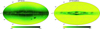 |
Fig. 1 All sky spatial distribution of our dataset. Initial cross-match of Gaia DR3 and AllWISE, i.e. ɡdr3wise shown in the left panel, and the red clump candidates selected from this are shown in the right panel, i.e. ɡdr3wise[RC] for the region |ZGC| < 2 kpc. |
2 Data
Our primary dataset is the official cross-match between Gaia DR3 and AllWISE, obtained from the all-wise_best_neighbour table provided on the Gaia data archive; the details of the cross-match algorithm are provided in Marrese et al. (2019)2. We retain only those sources with finite measurement for parallax (ϖ), as well as photometry in both Gaia (G) and AllWISE (W1 and W2) bands. This gives a count of N = 303 183 850 sources. The all-sky distribution of this dataset, which we call ɡdr3wise, is shown in Fig. 1 (left panel). Our algorithm to select RC stars is agnostic to the data quality; hence, at this stage we do not filter out poor data.
2.1 Photo-astrometric selection of the red clump
For each star, one can in principle compute the absolute magnitude (Mλ) in both the AllWISE (λ = W1) and Gaia (λ = G) passbands as
 (1)
(1)
where μ = 5 log10(100/ϖ′[mas]) is the distance modulus, and Αλ is the extinction in the passband λ, whose estimation is described in the following section. We adopt ϖ′ = ϖ + 0.017 assuming a global parallax offset from Lindegren et al. (2021). However, applying Eq. (1) would mean inverting the parallax to obtain an estimate for the distance modulus, which would yield problematic distances for sources with high parallax uncertainty, σϖ/ϖ > 0.2 (Bailer-Jones 2015; Luri et al. 2018). In this light, we make use of the Bayesian distances estimated by Bailer-Jones et al. (2021) [hereafter CBJ21]. Their catalogue provides geometric distances (dgeo) for 1.47 billion sources, requiring only the Gaia EDR3 parallaxes. Additionally, for a large majority, they also provide photo-geometric distances (dphotgeo) for sources where G magnitude and GBP – GRP colour are also available. In general, the photogeo distances are considered better for sources with high σϖ/ϖ. However, these have a dependence on the stellar population modelling in the Gaia EDR3 mock catalogue (Rybizki et al. 2020) used as a prior, and could have complex behaviour at low latitudes, as noted by CBJ21. In any case, both distance estimators are dependent on the assumed 3D density distribution of stars in the Milky Way, and in the case of CBJ21 this is derived from the Besançon Galactic model (Robin et al. 2003) used to construct the Gaia EDR3 mock catalogue of Rybizki et al. (2020). Following CBJ21, we construct the posterior probability distribution function (PDF hereafter) of distances (d) for every source in our sample. This can only be done for their geometric distances, and in any case our intention here is to use an informed prior with as few assumptions as possible, and only for the purpose of selecting RC candidates. We use the distance priors and a likelihood function (see Appendix B), to compute the PDF on a grid of 500 points (d1, d2, …dn), with d1 = 0, and dn = 2 × (dphotgeo|dgeo), i.e. setting the maximum grid point to be twice the distance prior for each source. In general, we use dphotgeo distances where available, but for the minority of sources that don’t have these provided, we use dgeo distances instead. We use the median value of the distance PDF, along with sky position (l, b) to estimate the reddening E(B – V), and using the reddening coefficients listed in Sect. 2.3 to convert to extinction Αλ.
We then converted the distance grid to that in absolute magnitude (i.e. Μλ,1, Μλ,2, …, Μλ,n), thus obtaining the posterior PDF in Μλ, to which we fit a broad Gaussian (𝒩) profile in order to obtain the peak and spread  in the inferred distribution. Since any given star has a single true absolute magnitude,
  quantifies our uncertainty on our inferred Μλ value, taken as the mean of the fitted Gaussian due to distance and extinction uncertainties. This procedure is illustrated in Fig. 2.
The absolute magnitude for the RC has been calibrated in several passbands, for example by Hawkins et al. (2017) and Ruiz-Dern et al. (2018), who also considered variations due to colour. Khanna et al. (2019, K19 hereafter) calibrated the absolute magnitude in the K band as a function of metallicity MK([FeH]) using the Galaxia code (Sharma et al. 2011). They showed that the dependence of MK on metallicity is non-negligible for stars with [Fe/H] < −0.4 dex, while beyond this metallicity, the MK is roughly flat with [Fe/H] (see their Fig. A.4). How many [Fe/H]< −0.4 RC stars we expect to observe depends on the age distribution, and the apparent magnitude limit of the sample. In Appendix C.2, we select RC stars from a Milky Way analogue generated using Galaxia. For these, Fig. 3 shows the distribution of MG versus (G – Rp)0, and MW1 versus (W1 – W2)0, with the locus of the RC marked by black contours. Figure C.4 shows the cumulative distribution function (CDF) of metallicity for the RC. We show the CDF profile for three different age caps, that is assuming the maximum age of the RC sample in the Galactic disc is τ = (5, 7, 10) Gyr. We find that the expected fraction of RC at [Fe/H] < −0.4 is about 12 % for a cap of τ < 7 Gyr, and reaches about 20% for τ < 10 Gyr. Since the age distribution of RC generally peaks around 1 ~ 2 Gyr (Girardi 2016), we do not expect many RC stars at [Fe/H] < −0.4 dex and thus neglected this small metallicity dependence in the absolute magnitude. Table 1 lists the absolute magnitude  and intrinsic dispersion
  for the RC in the photometric bands used here, according to Hawkins et al. (2017).
In order to select the RC, we assumed that the distribution in absolute magnitude space is a 2D Gaussian with the centroid at  . In general for a given distribution, the distance between its centroid (x0) and a point of interest (x1) can be given in terms of the Mahalanobis (1936, Dml) distance given as
 (2)
(2)
which respects the combined covariance (Σ) of x0 and x1. In our context, x0 and x1 are the two dimensional mean absolute magnitudes of the RC and of our inferred absolute magnitudes (MG,MW1). The covariance matrix is then given as
 (3)
(3)
where the diagonal terms combine the spread in the observed  and true dispersion of absolute magnitudes
  such that
  and likewise for W1 (we used ςg to avoid confusion with σG, the photometric uncertainty of G). The off-diagonal elements of Σ depend on the correlation (ρgw) between the absolute magnitudes in the two passbands inferred by us as well as between the absolute magnitudes in the two passbands for genuine RC stars. Since we have assumed the same distance prior and extinction map to derive the pdf of the absolute magnitudes in G and W1, the correlation between the inferred absolute magnitudes is very close to 1. In order to determine the correlation in the intrinsic absolute magnitudes of RC stars, we selected from adr3wise, stars with σϖ / ϖ < 0.05, for which we could determine the inverse parallax distance
  and hence the absolute magnitudes using Eq. (1) in both the passbands. We further retained only those stars for which
  , i.e. where the absolute magnitudes were consistent with literature values of the absolute magnitudes of RC stars to within 1σ. For this sample we could then compute the Pearson correlation coefficient between the predicted (and observed) apparent magnitudes (see Appendix A which turns out to be close to 0.4). This would suggest that the overall correlation has to be between 0.4 & 1.0, and we thus assumed a naive average of ρgw=0.7.
For a Ndim (=2 here) dataset, one can then write a likelihood function for every source in terms of the Mahalanobis distance as
 (4)
(4)
where |Σ| is the determinant of the covariance matrix. To select a source as an RC star, we require ln(L) > ln(L)th, where the threshold (L)th is set by considering a hypothetical RC star placed exactly at Dml=3 that is observationally ‘perfect’ in the sense that  (and likewise for W1). Then using Eq. (4) we derive ln(L)th.
Using the procedure above for each star in the ɡdr3wise dataset we find a total number of 9 761294 RC stars if we neglect the correlation (i.e. ρgw=0) in Eq. (3), and instead 10 269 109 RC stars with the correlation taken into account (ρgw=0.7). Hereafter adr3wise[RC] refers to the latter case unless otherwise specified. We find that over 97% of our sources have an Astro-metric Fidelity (AF) >0.5, which is typically considered to be a threshold for good quality astrometry (Rybizki et al. 2020).
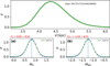 |
Fig. 2 Procedure to obtain the distribution of the absolute magnitude starting from distance priors illustrated for an example source. The top inset shows the distance prior used, which is turned into a grid of absolute magnitude using 3D extinction maps. The bottom figures show a Gaussian fit to the resulting absolute magnitude distributions in the G and W1 bands used to select the RC candidates. |
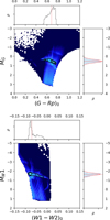 |
Fig. 3 Distribution of giants on the CaMD diagram in a mock realisation of the Milky Way using the Galaxia code (see Appendix C.2). The top panel shows MG vs Gaia colours, while the bottom panel shows MW1 versus AllWISE colours. The RC is marked by the black contours. The marginalised histogram (normalised) for the x (top sub panel) and y (right sub panel) axes are also shown. For the RC, both MG and MW1 can be approximated by a quasi-Gaussian as is shown by the red curves on the right insets. |
Absolute magnitude for RC stars.
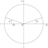 |
Fig. 4 Coordinate system adopted in this paper. |
2.2 Coordinate system
Our adopted coordinate system is illustrated in Fig. 4. We first transformed our (l, b) and distance, d, coordinates to heliocentric Cartesian coordinates, with the X-axis pointing towards the Galactic centre:
 (5)
(5)
To transform these heliocentric coordinates to galactocentric Cartesian coordinates, we assumed R⊙ = 8277 ± 9(stat) ±30(sys) pc from the ESO Gravity project’s most recent measurement of the orbit of the star S2 around the Milky Way’s supermassive black hole (GRAVITY Collaboration 2021). The heliocentric Cartesian frame is then related to galactocentric one by a simple translation: Xhc = XGC + R⊙, Yhc = YGC and Zhc = ZGC – Z⊙. The galactocentric cylindrical radius R is trivially found from  , while the cylindrical coordinate angle ϕ = tan−1(YGC / XGC) increases in the anti-clockwise direction, while the rotation of the Galaxy is clockwise, as seen from the north. The height of the Sun above the Galactic plane is adopted as Z⊙ = 0 pc (Gaia Collaboration 2023, hereafter Gaia23), though we found that our results remain unchanged even when we used the alternative Z⊙= 27 pc (Bennett & Bovy 2019).The uncertainties in our transformed coordinates are dominated by the uncertainties in distance estimates. We do not propagate these through the coordinate transformation, but instead generate multiple realisations of the data, each time sampling distances from the underlying distribution (see Sect. 2.4).
2.3 3D Extinction maps
In order to compute the absolute magnitude, we need good estimates of the extinction Aλ in passband λ. The widely used maps of reddening, E(B – V), from Schlegel et al. (1998, hereafter S98), estimates the extinction at infinity given a star’s 2D (l, b) sky coordinates. While these dust maps cover the entire sky, the 2D extinction values will overestimate the reddening for sources that are not outside the ISM layer. This can be improved upon by using 3D dust maps that require a prior for distances. All stars in our sample have a measured parallax, so in principle one could use this as a prior to estimate the distance, but as discussed earlier, instead we make use of the distances from CBJ21, as our purpose here is only to use these initial distance estimates to arrive at a realistic first-estimate of the foreground extinction along a given line of sight. For the selected sample of RC stars, we derived the distances independently, as described in Sect. 2.4.
At the time of running our algorithm, we had access to the following publicly available 3D dust maps: a) The Lallement et al. (2019) map3, derived with Gaia and 2MASS photometry and Gaia astrometry. This map provides the Gaia extinction parameter A0, defined as the monochromatic extinction at 541.4 nm at a resolution of 5 parsec within 3 kpc from the Sun and within 0.5 kpc perpendicular to the plane. b) Further out, we make use of the Bayestar 3D extinction map by Green et al. (2019). This is based on a Bayesian scheme, combining Gaia DR2 parallax with photometry from 2MASS and Pan-STARRS surveys. The spatial coverage is limited to the sky north of declination (dec) of −30°. For each source, we multiply the Bayestar map output by a multiplicative factor to obtain the reddening, i.e. E(B – V) = 0.884 × E(Baye star 19), as recommended4. c) For the remainder of the sky, we return to the S98 map, but in order to correct for the overestimation in the extinction, we estimate a dust fraction factor (following Koppelman & Helmi 2021) as
![Mathematical equation: ${{{E_{B - V}}\left( {l,b,s} \right)} \over {{E_{B - V,\infty }}\left( {l,b} \right)}} = {{\mathop \smallint \limits_0^s \rho \left[ {x\left( {s\prime } \right)} \right]ds\prime } \over {\mathop \smallint \limits_0^\infty \rho \left[ {x\left( {s\prime } \right)} \right]ds\prime }},$](/articles/aa/full_html/2025/09/aa52798-24/aa52798-24-eq22.png) (6)
(6)
where EB–V,∞(l, b) is the extinction estimate from S98, s is the heliocentric distance to a source, and x is the position vector. We note that ρ(R, ɀ) is the dust density model, which we adopted in this case from Sharma et al. (2011):
 (7)
(7)
with the disc warping and flaring (fl) modelled as
 (8)
(8)
The parameters of the model are from Robin et al. (2003) and listed in Table 2. In the AllWISE bands, we adopted the following reddening coefficients: AW1/E(B–V) = 0.174 and AW2/E(B–V) = 0.107 (Sharma et al. 2011). Using the dustap-prox code, we applied the mid-IR extinction curve from Gordon et al. (2023) and adopted R(V) = 3.1 to compute the ratios, AW1/AG = 0.07, AW1/ABp = 0.05, and AW1/ARp = 0.09, which is appropriate for a typical red clump star (4200 < Teff < 5400 K, 1.8 <log ɡ < 3.2). We find that these ratios are insensitive to [Fe/H].
2.4 Red clump distance and uncertainty
For every star classified as RC and assumed as having an absolute magnitude Μλ as per Table 1, we can invert Eq. (1) to calculate the distance modulus, but since the extinction Aλ itself depends on the distance, we follow an iterative procedure instead. First, we derived the maximum possible distance modulus for a star, assuming zero extinction along the line of sight,
 (9)
(9)
Using this equation, we could in turn derive the maximum distance (dmax), then compute the extinction, Aλ(l, b, dmax)i, and ultimately compute an updated distance modulus,
 (10)
(10)
Using μi we then recompute Aλ(l, b, d)i, and repeat the procedure until the distance modulus is converged (typically within five iterations) to  . For every star we sample the absolute magnitude from a Gaussian
  , using the values listed in Table 1, to derive the PDF of the distance modulus.
From Eq. (9), we can consider two main sources of uncertainty in our distance estimate, (a)  : The intrinsic dispersion in the absolute magnitude, and (b)
  : The photometric uncertainty. From Table 1, we see that
  is twice as large in the G band (0.2mag) compared to that in W1 (0.1mag). For this reason, we decided to use only the distances based on W1 passband in order to minimise the distance uncertainty and the effects of extinction. As for photometric uncertainty, we find that about 99.5% of our RC sample has σW1 < 0.1. In fact Fig. 5(b) shows that the overall σW1 << 0.1, i.e. the photometric uncertainties are generally much smaller compared to the intrinsic dispersion in the absolute magnitude in W1. We exclude the remaining 0.5% of the sources that have σW1 > 0.1, though given their insignificant number, their removal or not makes no noticeable difference in the results. For every star, we combined the two sources of uncertainty in quadrature to derive the uncertainty in the distance modulus as
 (11)
(11)
Strictly, one should also consider the uncertainties in the extinction maps, but since in this contribution we use a combination of various maps, this is not a trivial exercise, and we ignore it for simplicity. However, since we use primarily the distances based on W1, we anticipate this to be a small effect. We assume the uncertainties in the distance modulus are Gaussian, i.e.  . It can be shown then that the typical uncertainty in the photometric distance (d) is,
  , while a naive inversion of the parallax results in distance error given by
  , where σϖ is the parallax error. Figure 5a compares the profiles of the distance uncertainty with respect to distance from the two approaches, showing that beyond a heliocentric distance of about 3 kpc, the RC distances are superior.
Dust model parameters.
2.5 RC catalogue and validation
In Fig. 1, we show the full sky distribution (l, b) at healpix level 5, for the ɡdr3wise crossmatch (left panel), and for the selected RC candidates (right panel). The apparent magnitude distribution of the selected RC sample is shown in Fig. 6, where we note the faint limits (99.5 percentile) at mG,lim=17.5, and mW1,lim=13.8. We also note that A11WISE is essentially complete in this magnitude range (Schlafly et al. 2019, see their Fig. 4). We show in Fig. 7, the colour-magnitude distribution (grey) for the ɡdr3wise parent sample in both Gaia and A11WISE colours. In each panel, the bifurcation between Giants and dwarfs is apparent, and indicated in red contours is the region occupied by our selected RC sample.
Most of the selected sources are confined within |b| < 10° of the plane, but our algorithm also picked out sources around the Large (LMC) and the Small (SMC) Magellanic clouds. The LMC (RA, DEC = 81.28, −69.78) is known be at a distance of about 50 kpc from the Sun (Pietrzyński et al. 2019). Along this line of sight, we estimate extinction of AW1 = 0.15, and AG = 2.38. From Eq. (1), we would then expect the brightest RC in the LMC to be visible at G = 21.3 or W1 = 16.9, which lie outside the magnitude distribution of our RC candidates. Instead, these sources enter the selection because the CBJ21 catalogue has no priors for LMC/SMC stars, and since the relative parallax uncertainty is high for these sources, they are assigned incorrect distances. Our goal is to primarily select RC stars in the Milky Way disc, so for density modelling, we restrict our final sample to the region |ZGC| <2 kpc which also removes the contamination at b > −30° from the Magellanic clouds, as in Fig. 1. Though we note that the results remain changed even without this cut, because of the very low relative contamination from these stars to the total number of about ten million.
In Fig. 8a, we show the density maps for this dataset in the galactocentric XGC–YGC projection, showing clearly the region in the inner Galaxy (R<3 kpc) that we mask. Our sample provides a good coverage between 3 < R < 14 kpc. Figure 8b shows the corresponding YGC–ZGC projection to show the extent of the coverage vertically with regard to the midplane of the disc. This is also illustrated in Fig. 9, where it is clear that most of the sample lies within |ZGC| < 1.5 kpc, and that towards the outer disc (R > 10 kpc) there is a hint of flaring in the vertical counts. To see this more clearly, in Fig. 10a we plot the number counts as a function of ZGC at successive R annuli, spanning from 3 to 17 kpc. The slope of the profiles is a measure of the scale height of the disc at a particular annulus, while a change in the slope from the inner to the outer disc would indicate a change in the scale height, thus flaring if the scale height increases with R. Figure 10b shows the vertical number counts folded along the ZGC axis (i.e. |ZGC|), which makes it easier to spot the changing slope with R, in particular beyond R = 11 kpc. We remind the reader, however, that Fig. 10 shows the vertical counts in the data without accounting for the selection function, and therefore fitting a model (for example an exponential) directly to this figure is not appropriate. Here we are simply presenting the data for a visual inspection, and note the hints of a flared disc.
Any scheme for the selection of the RC based purely on astrometry and photometry is bound to have contamination from neighbouring populations. This is mainly due to limitations such as the quality of extinction maps, and uncertainty in photometry and parallax. Also, in the case of the RC, intrinsic colour and magnitude are not enough to separate such stars from red giant branch (RGB) stars occupying the same part of the HRD. In such cases, however, while not true RC stars, their true photometric distances will not be too different than those of the true RC. Since we are able to select a very large sample of RC candidates, we carry out a comparison with a few spectroscopic (GALAH and APOGEE), and asteroseismic catalogues for validation in Appendix C. For the stars that are found in common with these catalogues, we find that their distribution in the Kiel (Fig. C.3), colour–magnitude (Fig. C.1), and colour–absolute–magnitude diagrams (Fig. C.2, is reasonable for our RC sample.
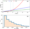 |
Fig. 5 Panel a: typical distance uncertainty for the red clump as a function of distance. The red curve shows the expectation from a naive inverse parallax estimation, the blue curve shows the predicted uncertainties in the photometric distances in G band and for W1 this is shown by the green curve. The two vertical dotted lines indicate roughly the distances beyond which the photometric distances become more informative than parallax inversion for the two bands. Panel b: distribution of photometric uncertainty in W1 for the RC stars shows that σw1 ≪ 0.1, i.e. lower than the intrinsic dispersion in the absolute magnitude of RC stars in W1. |
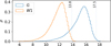 |
Fig. 6 Apparent magnitude distribution of the ɡdr3wise[RC] sample in the G and W1 bands. The vertical dashed lines at G=17.5 and Wl = 13.8 indicate the 99.5th percentiles in the respective bands. |
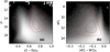 |
Fig. 7 Colour magnitude diagram for the ɡdr3wise parent catalogue shown in gray for Gaia and A11WISE colours. In each panel, we indicate the selected RC sample using the red contours (1σ, 2σ). |
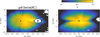 |
Fig. 8 Spatial distribution of the ɡdr3wise[RC] sample for the region considered for model fitting. Panel a shows the galactocentric XGC–YGC projection, with the location of the Sun (black star) and the Galactic centre (black dot) also indicated. Stars within R < 3kpc of the Galactic centre have been removed. Panel b shows the corresponding galactocentric YGC–ZGC projection. The number density is shown on a logarithmic scale. |
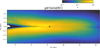 |
Fig. 9 Galactocentric R–ZGC projection for the ɡdr3wise[RC] sample over the region considered for our model fitting. The number density is shown on a logarithmic scale. The location of the Sun is indicated as a black star. |
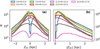 |
Fig. 10 Vertical counts of ɡdr3wise[RC] for successive annuli in R between 3 and 15 kpc. Panel a shows the counts as a function of ZGC, while panel b shows the same folded along the vertical axis, i.e. |ZGC|. In panel b, a change of slope in the vertical counts is evident as we move from the inner to the outer disc region. |
3 Method
3.1 Modelling the Galactic disc
The number density distribution, N(R, ɀ), in our model is described by two exponential discs, each of the form
 (12)
(12)
with scale height (hɀ), scale length (Rd), and an inner-cut radius (Rcut), which excludes the region not described by the disc, such as in the inner Galaxy (Aumer & Binney 2017; Vasiliev 2018). The disc is exponentially flared, i.e. hɀ increases with R, controlled by the flare scale length, Rfl,
 (13)
(13)
with scale height normalisation, hZ,⊙, at the solar radius R⊙. The total density is thus given by
 (14)
(14)
with fd1 being the mass contribution of the first disc. The density function is normalised such that over the observed volume fV F × N(R, ɀ)dV = Nobserved, where the fraction of observable stars is in the range of F = [0, 1] (see Sect. 3.2). We also considered a warped disc in one of the components. This we parametrised as
 (15)
(15)
where the onset of the warp is at Rw (i.e. ɀw= 0 inside this radius), and its amplitude is set by hw0. The warp is sinusoidal such that the line of nodes lies along ϕ′ = ϕw, where,  , being zero towards the anticenter and increasing in the direction of Galactic rotation. We distinguish this from the galactic azimuth, ϕ = tan−1(YGC/XGC), which instead increases anti-clockwise (see Fig. 4). We do so to both be consistent with standard coordinate frame conventions, as well as those preferred by the warp modelling papers.
The Milky Way is known to host a bar, and over the past several years, the range of the bar length (3 < Rb < 5 kpc) has been estimated using various tracers (Gaia23 and references within). For our purpose we retained as much of the disc region as possible while removing the probable regions most affected due to the central bar. Recently, Vislosky et al. (2024) estimated a value of Rb = 3.6 kpc but suggest that it could be as low as 3 kpc. For this reason, we fixed the inner-cut radius, Rcut = 3 kpc. Our tests showed that increasing Rcut to 3.5 kpc barely impacted the results, so we chose to stick to the lower bound of Rb. For our RC sample, the ϕ–R projection is shown in Fig. 11. Our full model fits for a maximum of 10 parameters. These are the scale parameters of the first disc (Rd, hɀ,⊙, Rfl), and its mass fraction (fd1), and four parameters describing the warp (ϕw0, Rw, aw, hw0), and the scale parameters of the second disc (Rd2, hɀ2,⊙). We only allow the first disc to be warped and flared. Our initial exploration of the observational data showed no major difference if both disc components were allowed to be both flared and warped, so in order to reduce the parameter space and degeneracy between parameters, we imposed this condition. All the parameters we fit for are listed in Table 3, along with their bounds and units.
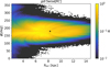 |
Fig. 11 Spatial distribution in the ϕ–R projection of the observational red clump sample constructed from the ɡdr3wise parent dataset. The range shown here is the region over which we performed our model fitting. |
Description of Galactic structure parameters.
3.2 Selection function
Here, we discuss the various layers of the selection function that need to be accounted for in our modelling of the observational data. If we consider stars in a 3D grid in space, in this case in XGC × YGC × ZGC, our goal is to be able to predict the number counts in each voxel, i:
 (16)
(16)
where Si[0, 1] is the correction factor (selection function) to the counts predicted by the model, Ni,true. In the ideal case, Si would be equal to 1 if we are able to observe the entire ground truth, that is, all stars of our modelled population in a given voxel, i. In the worst case, it would be 0 if there was missing or poor quality data in some patches of the sky but also if the survey is not designed to observe certain fields. In our specific case, Si is the fraction of the RC stars in voxel i that can be seen for our sample. However, we point out that in general, the selection function is dependent on observable quantities (Rix & Bovy 2013; Frankel et al. 2020), and here we can only define an Si for a given voxel, i, and interpret it as the fraction of stars in that voxel because we are dealing with a standard candle, which allows us to translate the observed apparent magnitude into a distance once we assume an extinction map. We can set out two principle layers that determine Si:
(a) Effective volume: For a magnitude limited survey, (mλ < mλ,lim), for a quasi-fixed absolute magnitude, such as is the case with the RC, we can define a maximum distance modulus (μ),
 (17)
(17)
such that from our position at the Sun, the observable volume would be traced by a sphere with a radius (dmax) corresponding to this maximum distance modulus. However, here we neglect the presence of interstellar dust, which is an unavoidable evil in the Galaxy. When accounting for it, the maximum distance modulus μ_max is no longer a constant and instead varies for each voxel i:
 (18)
(18)
Consequently, the observable or effective volume is crumpled and no longer a simple sphere, as illustrated in Fig. 12. Essentially, this is similar to integrating a density function over the whole sky, but with the limits on distance varying by line of sight. Hence, depending on the dust distribution, the limit of the volume sampled varies in different directions on the sky. Along some lines-of-sight one can only map to a few kiloparsecs, while along others it is possible to map out the edge of the Galactic disc. Thus we need to take into account this dust/mλ,lim induced distance limit.
Since we are modelling the number counts on a fixed 3D grid, we must also take into account the finite size of our voxels. We can pre-compute the fractional effective volume, Fi, for each volume element (ie. voxel), and then apply it to both simulated and observational data. For example, let us consider a cube shaped grid (XGC × YGC × ZGC), where every voxel has the same size, and is small enough such that the median heliocentric distance of all stars in that voxel can be approximated by the median heliocentric distance of that voxel. Then for every voxel (l, b, di) we can check if di < dmax(l, b) (dmax condition), and retain only those that satisfy this condition. However, for nearby voxels the size of the voxel may be significant with respect to its heliocentric distance, or the extinction may vary significantly within a voxel. In this case, the median quantities of the voxel (li, bi, di) are not representative of the median quantities of the stars within it. This becomes more of an issue if the volume elements of the adopted grid do not have a fixed size. In this work, because the number of stars decrease exponentially with galactocentric radius, to increase the statistical significance of the counts per voxel in the outer disk, we adopt a cylindrical grid (R,ϕ,ZGC), so that the volume of the voxels increase with R, fixing the cylindrical grid to the binning (ΔR,Δϕ,ΔZGC) = (0.25 kpc, 10°, 0.25 kpc), from Rmin=3 to 20 kpc in radius, 0 to 360° in ϕ, and between ±2 kpc in ZGC.
As an example let’s first consider such a cylindrical grid where for every voxel we compute the heliocentric distance at its centre. Then we assume a single absolute magnitude MG = 0.44 for our RC stars, so that for a given magnitude limit (say G = 16), we can estimate the dmax. In Fig. 13 we consider the case without extinction, so dmax is a constant (12.94 kpc), and at ZGC=0 kpc, i.e. right in the midplane. Figure 13a–c show the ϕ versus R projection of the voxels, mapped by different quantities. Figure 13c shows the projection mapped onto heliocentric distance, only for those voxels that satisfy di < dmax (using the centre of the voxel). So it follows that in Fig. 13b, all voxels outside of this condition have Fi set equal to 0; that is, no RC stars in this volume element will be in our magnitude limited sample. In contrast, those inside have Fi set equal to 1; that is, the selection function resulting from the magnitude limit is binary, as expected.
To check if this approximation is valid, we sub-bin our 3D cylindrical grid by a factor of 5 in each dimension (125 sub-voxels) and then in each voxel we can count the number of sub-voxels that satisfy the dmax condition, to now obtain a fractional selection function (Nd<dmax/125 instead of a binary 0 or 1). Figure 13a shows the ϕ versus R mapped in the midplane by this corrected selection, which we can now compare it to the previous simple binary selection in Fig. 13b. We can see that while for most voxels the correct selection function is identical to that in Fig. 13b (= 0 or 1), there is a set of voxels along the edge (where d = dmax) where some fraction of the voxel is still observable. Thus the sub-binning approach allows us to account for estimating the effective volume of a voxel and correctly include this region in our model.
This effect is drastic in the presence of dust, as is illustrated in Fig. 14, where again we show the projection of voxels in ϕ versus R. In panel b, we show all the voxels that should be observable but colour-coded by the incorrect binary selection function that does not take into account the finite size of the voxels. All the voxels coloured red have a selection probability of 1, while those in blue have a selection probability of 0 in the incorrect approach; thus only the red voxels would have been predicted to be observable. In panel a, the same voxels are presented but instead colour-coded using the correct method, now also taking into account the extinction to each sub-voxel when checking if its distance is within dmax. Now instead of having a binary 1 or 0, the voxels have a continuous selection fraction between 0 and 1. This approach would then correctly predict some of the blue voxels from panel b to be truly observable, while some of the red voxels are only partially observable.
Figure 14 illustrates the non-intuitive pattern that the variation of Galactic dust imposes on the region observable in the Milky Way.
Henceforth for all our analysis, we use the sub-binning method described above to estimate the effective (fractional) volume of each voxel. For the observational data, we use the magnitude limit in the G band 17.5 from Fig. 6, and the absolute magnitude is sampled from a Gaussian, that is, the luminosity function of the RC is taken as  , where
  is taken from Table 1. Thus compute the first layer of the selection function given as the fractional effective volume of each voxel as
 (19)
(19)
(b) Gaia selection function: Apart from the probability that an RC-like star can be observed given the magnitude limit of our sample, we also need to consider the probability that a source can be observed by Gaia at all. We term this the top-level selection function (S top,i). Cantat-Gaudin et al. (2023) modelled the completeness of Gaia by comparing to the much deeper DECAPS survey (Schlafly et al. 2018). They were able to devise a single parameter called M10 that encapsulates the completeness based on only three observables, the sky position and magnitude (l, b, G). For our grid, we can compute the M10 for every voxel using the aforementioned sub-binning approach and thus get the top-level selection function for every sub-voxel. We do this by using the GaiaUnlimited Python package5, and the class DR3SelectionFunctionTCG, using the central values of (l,b,G) in each sub-voxel. In any case, given our G magnitude limit of 17.5, Stop,i will be equal to 1, except in the most crowded fields.
Our parent dataset ɡdr3wise is a cross-match between the Gaia and AllWISE surveys. More specifically, every source in our parent catalogue is present in Gaia, and we are using the subset of stars that also have AllWISE photometry. In addition, we require that our stars have a measured parallax, so in summary we require all stars to have a finite (l, b, ϖ, G, W1). Essentially, all these filters are introducing selection effects of their own. To account for this we can compare the number of stars in the catalogue before and after applying the selection criteria in bins of Gaia observables. This characterises the completeness as a function of quantities such as sky position and G magnitude. This ratio-ing method allows us to build a sub-selection function (since we can safely assume every source we study here is observed by our principal survey Gaia). Castro-Ginard et al. (2023) developed such a methodology to estimate the selection function for different subsamples of stars in the Gaia catalogue. This is done by comparing the number of stars in a given subsample to that in the overall Gaia catalogue, providing an estimate of the subsample membership probability (S sub,i) as a function of observables of choice. In the GaiaUnlimited code, the SubsampleSelectionFunction class uses a beta-binomial estimator to convert the number count ratios into a probability for a source to end up in the subsample. We choose to compute the ratios in bins of sky position and magnitude (l,b,G) only. In Appendix D, we show the query that is run on the Gaia archive that allows us to compute this sub-selection function, and we show in Fig. D.1, the sky projection of the completeness for a bright (12< G < 13) and a faint 16 < G < 17 magnitude bin at HEALPix level 5. The sub-selection function estimator relies on binning and computing number ratios, so naturally the more dimensions one would bin data in, the fewer stars there would be per bin, thus increasing the variance in the estimated selection function. We find that the selection function for the RC hardly varies with colour (G – Rp), and so ignoring this dimension allows us to have a more robust number statistic on the sub-selection function. The overall selection function is then a product of the individual layers,
 (20)
(20)
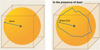 |
Fig. 12 Illustration of the maximum observable distance (dmax) for the RC for a magnitude-limited survey. The left panel shows the ideal situation when there is no dust extinction, in which case the observable region traces out a sphere with radius dmax. On the right is shown the case with extinction, which depends on the sky position (l, b) due to which dmax(l, b) varies across the sky and modifies the effective volume from that of a perfect sphere. |
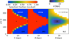 |
Fig. 13 Illustration of the selection function projected in ϕ–R space for the case without dust at ZGC=0 kpc (midplane). Panel a shows the map of the selection fraction computed using the sub-binning method, panel b shows the same for the method without sub-binning, while panel c shows the distance to all voxels that are within a distance of dmax < 12.94 kpc of the Sun. Panel a also shows the additional voxels that would be missed by assuming the median values of observables (l, b, G). In all panels, the location of the Sun is indicated by the black star. |
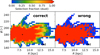 |
Fig. 14 Illustration of the effective volume projected in ϕ–R space for the case with dust. Panel a shows the map of the selection fraction computed using the sub-binning method, and it shows a continuum of probability between 0 (unobservable) and 1 (fully observable). In panel b, we show the same voxels as in panel a, but for these the selection fraction is shown for the method without sub-binning. This shows that several voxels from panel a that have a probability of being observed would be considered unobservable or would be completely observed using the incorrect method of estimating the selection function. In both panels, the location of the Sun is indicated by the black star. |
3.3 Generating mock data
For the purpose of validating our methodology, we generate mock datasets for which we know the true values. These are simplified models whose formulations are consistent with our model assumptions and thus ideal test cases for validating our procedure.
For a given density model, the total number of stars can be computed by integrating over the volume of the survey,
![Mathematical equation: $N = \mathop \smallint \nolimits^ N\left( {\left[ {R,z} \right]\left( {l,b,\mu } \right)|\Theta } \right) \times {{d_{hc}^3log\left( {10} \right)} \over 5} \times {S_i}\,\,\,d\mu dldb,$](/articles/aa/full_html/2025/09/aa52798-24/aa52798-24-eq48.png) (21)
(21)
where N([R, ɀ](l, b, μ)|Θ) is the number density as before but for a given line of sight (l, b) and at distance modulus μ. To generate a mock catalogue, we sample (l, sin(b), μ) from the density models and thus need the Jacobian  . The Si is the effective selection function of the mock catalogue. For example, if we generated a mock that is magnitude limited, has a sky dependent selection function, and is restricted only to the red clump, the net selection function would be
 (22)
(22)
where LFRC is the luminosity function (absolute magnitude distribution) of the red clump. In Fig. 3, we showed the caMD distribution of the RC from Galaxia. The marginalised distribution of absolute magnitude (right insets) shows that both MG and MW1 can be approximated as quasi-Gaussian. Therefore, for the rest of the paper, we adopt a Gaussian LFRC,  , using values from Table 1. One could also simplify the method by adopting a delta function,
  , in which case we would assume all RC to have a singular absolute magnitude.
We use the multidimensional sampler, sampleNdim, from the AGAMA code (Vasiliev 2019) to then generate our mock catalogue of one million sources. We convert from the heliocentric to the galactocentric frame, as described in Sect. 2.2, but for the mock we here assume Z⊙= 0 kpc. In Sect. 4.1 we generated several versions of the mock catalogue, to demonstrate how our model fitting methodology performs for a range of Galactic parameters, magnitude limits as well as with and without having applied extinction.
3.4 Fitting
We first grid all data in 3D space (ΔR,Δϕ,ΔZGC)= (0.25kpc, 10°, 0.25kpc) kpc. Then, using the model described in Sect. 3.1, we predict the counts in each bin Ni,raw. These “raw” counts predicted by the model need to be corrected, taking into account the selection function, i.e. Ni = Ni,raw × Si. Then we compared the predicted and the observed counts per bin by maximising a Poisson log-likelihood (Bennett & Bovy 2019),
![Mathematical equation: $lnp\left( {{N_{obs}}|N} \right) = \mathop \sum \limits_i \left[ { - {N_i} + {N_{obs,i}}ln\left( {{N_i}} \right)} \right],$](/articles/aa/full_html/2025/09/aa52798-24/aa52798-24-eq53.png) (23)
(23)
with the emcee package (Foreman-Mackey et al. 2013). We used max(25,7 × Ndim) walkers and up to 5000 iterations. We performed the model fitting only over those voxels with Nobs,i > Nmin,i, i.e. with counts above a minimum threshold. For the mock data, we generated one million particles in all and used Nmin,i=10, while since the observational dataset is of the order of ten million stars, there we varied Nmin,i=(20,… ,50) in order to estimate the uncertainties in our parameters (see Sect. 4.2.2). In order to visualise our best-fit, we inspected two dimensional projections of the number counts. Specifically, we compared the surface density Σsur f versus R for the data and the model in bins of ΔR = 0.25 kpc in order to inspect the radial profile of number counts. Similarly, we compared N(ɀ|R) versus ZGC for the data and the model in bins of ΔZGC = 0.25 kpc at different R in order to inspect the vertical profile. Finally, we considered the projection in ϕ-ZGC at various R, moving from the inner to the outer disc. This was done to inspect if our model is able to fit azimuthally varying features in the data.
4 Results: Density modelling
4.1 Fitting mock data
We begin this section by demonstrating our model fitting method on a mock catalogue of RC stars that were generated as described in Sect. 3.3. We tested our method on several different test cases, but for the demonstration we here restrict ourselves to the two cases discussed below. In both cases, we only consider the selection function layer due to extinction and the top level Gaia selection function since the sub-sample selection does not apply to our simple mock density model. The demonstration is also made available as a GitHub notebook6.
Case I: We generated a mock galaxy of one million particles with a one-disc component and no warp. The density profile is described by an exponential in both R and ZGC. Additionally, this galaxy has a flare, and we impose a magnitude limit of G=17.5. In order to exaggerate the effects of extinction we choose to use here the 2D dust model of S98 instead of the 3D model described in Sect. 2.3. Finally, we convolve the simulated distance modulus (μ), with typical RC distance uncertainties (see Sect. 2.4). The true parameters for this disc are (Rd, hZ,⊙, log10 Rfl[kpc])=(3.3 kpc, 0.3 kpc, 0.6). The density maps of the mock are shown in Fig. 15, with the projection in galactic coordinates (l, b) in panel a in R–ZGC (to show the flare) in panel b, and in Cartesian galactocentric coordinates (XGC,YGC,ZGC) in panels c and d. In Fig. E.1, we show the corner plot from the MCMC fitting carried out for this example disc, where we had set Nmin,i=10. The best-fit values are indicated with vertical lines, and agree very well with the input values for the mock. To better judge the fit, we also show the projection in ϕ–ZGC space in Fig. 16 of the mock data and the fitted model for galactocentric radial bins between 4 < R < 8.5 kpc (columns 1 and 2). Also shown in Fig. 16 are the residuals between the mock data and model (column 3). The colour map of the residuals shows general good agreement except at the edges of the density distribution where the number of stars drops rapidly.
Case II: The second example we include is that of a disc which is warped, described by (ϕw, Rw, aw, hw0)=(170°, 6.5 kpc, 1.0, 0.3 kpc). This is a rather extreme warp ideally oriented for the purpose of illustration and testing, and is not meant to represent the warp of the Milky Way. The rest of the parameters are identical to the disc in case I. Figure 17 shows the density maps for this mock data, where a tilt (top left to bottom right) is apparent in the (l, b) map in panel a. This can be compared to Fig. 15a where the disc was not warped. In Cartesian coordinates, the sense of the warp here is such that the disc bends up (towards positive ZGC) at positive YGC, and bends down at negative YGC, as shown in Fig. 17, as expected for the line-of-nodes being at ϕ = 170°. Figure E.2 shows the corner plot of the fit, again with the best-fit values indicated as blue lines. The MCMC procedure converges to recover the input values, although we did notice that the warp parameters (Rw, hw0 and aw) show strong correlations between them. The ϕ-ZGC projection of this dataset is also shown in Fig. 18, again for three successive bins in R, though here we note that the density map shows a diagonal feature beyond R> 7 kpc that is the imprint of the warp. The residual maps are again mostly close to zero across the pixels, except at the very edges (low number statistics), and thus show that the fitting works well in this case too, and we are able to fit both for the structural (scale length and height) and shape parameters (warp) of the disc, though these later show significant correlations.
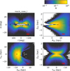 |
Fig. 15 Mock case I: density distribution for the example with a single exponential disc that is also flared for magnitude limit G = 17.5. A dust model was applied to the sample, as is evident in galactic coordinates (l, b) in panel a with the gap at very low latitudes. Panels b, c, and d show the corresponding spatial distribution in Cartesian galactocentric coordinates. The locations of the Sun (star) and Galactic centre (dot) are indicated by black points. |
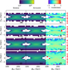 |
Fig. 16 Mock case I: fitting residuals shown in the ϕ-ZGC projection. Panel a shows the number density (logarithmic scale) of the mock data, panel b shows the predicted number density of the best-fitted model, and panel c shows the residual (relative to mock data). Panels a–c are restricted to 4 <R< 5.5 kpc. The subsequent rows show the same information but for selected successive bins in R. |
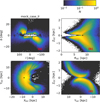 |
Fig. 17 Mock case II: density distribution for the example with a single exponential disc that is also both flared and warped for magnitude limit G=17.5. A dust model has been applied to the sample, as is evident in galactic coordinates (l, b) in panel a with the gap at very low latitudes. Panels b, c, and d show the corresponding spatial distribution in Cartesian galactocentric coordinates. The locations of the Sun (star) and Galactic center (dot) are indicated by black points. |
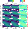 |
Fig. 18 Mock case II: fitting residuals shown in ϕ-ZGC projection. Panel a shows the number density (logarithmic scale) of the mock data, panel b shows the predicted number density of the best-fitted model, and panel c shows the residual (relative to mock data). Panels a–c are restricted to 6<R<7.5 kpc. The subsequent rows show the same information but for selected successive bins in R. |
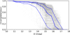 |
Fig. 19 Completeness for the RC sample for R >3 kpc, shown in gray, as a function of G magnitude (0.5 mag bins). The blue solid line shows the median profile, and the dotted lines show the 84th and 16th percentiles. |
4.2 Observational data
4.2.1 Selection function and completeness map
We move on to fitting our model on the ɡdr3wise [RC] dataset. Following Sect. 3.2, we apply all three layers of the selection function to the real data. The predicted completeness of the RC sample as a function of G magnitude is shown in Fig. 19, with the solid blue line indicating the median profile and dotted lines showing the variance in completeness. As this profile (blue line) is averaged over the entire volume (grid), we expect to see variance at any given radius. Overall, the RC sample is largely complete (close to 1) down to about G = 14, falls to about 0.5 completeness at G = 16, and then drops sharply to 0 by G = 17.
As mentioned in Sect. 3.2, taking advantage that RC stars are standard candles, we can determine the fraction of RC stars in our sample (completeness) for any particular volume. In Fig. 20, we show the completeness in polar coordinates (R,ϕ), averaged over three different slices in ZGC. Towards the inner Galaxy, the completeness drops sharply due to extinction, while in the anticentre direction the completeness extends much further. While overall the two maps at ZGC>0.25 kpc and ZGC < −0.25 kpc exhibit very similar completeness, there are minor differences between the two due to the asymmetrical dust distribution above and below the disc. Figure 20b shows the completeness for the midplane region, |ZGC | < 0.25 kpc. Compared to the maps at higher ZGC, the region of high completeness covers a much smaller region. Indeed, in the plane we are most affected by dust, which obscures our view towards the inner Galaxy and along other lines of sight with high extinction. In addition, we are also affected by high source crowding towards the Galactic centre, which makes it difficult for AllWISE to resolve individual sources and causes these fields to be less well sampled. Nevertheless, all three maps show that we are able to map out a large portion of the disc out to at least R= 15 kpc with fairly high completeness. An interactive three-dimensional visualisation of completeness for our RC sample is provided on the GaiaUnlimited webpage7.
4.2.2 Fitting model to data
Following the method used for the mock catalogues, we fit for the parameters listed in Table 3. In the first instance, we ignore the warp and check if we can fit the distribution with only a single flaring disc (i.e. we set fd1= 1). An example corner plot for this fit is shown in Fig. F.2, where we find, Rd= 3.13 ± 0.20 kpc, hɀ = 0.46 ± 0.02 kpc, and log10 Rfl= 2.14 ± 0.20. These are typical scale parameters for the old thin disc population Milky Way (e.g.. Bland-Hawthorn & Gerhard 2016), but in this case we obtain a slightly higher hɀ which compensates for a very weak flare. While the fit does converge, a closer look at the residuals shows that a single disc is not enough to account for the stellar density both in the inner (3 <R< 10 kpc), and the outer disc (10 < R < 15 kpc) simultaneously (see Fig. F.1). We therefore allowed for an additional disc component and fit for all the parameters (barring the warp again) listed in Table 3. An example corner plot in Fig. G.1, shows that the fit converges. Essentially, we find that the RC sample is best described by a two disc component model, with one component having Rd = 4.08 ± 0.32 kpc, hɀ = 0.18 ± 0.01 kpc, and log10 Rfl = 0.36 ± 0.04. This is essentially a disc with a long scale length exhibiting a strong flare, and constitutes about 34% of the total mass. The second component is dominant (~66%) has a scale length of Rd2 = 2.66 ± 0.11 kpc and constant (non-flaring) scale height of hɀ2 = 0.48 ± 0.11 kpc. When we included a flare parameter for this second disc, the fit was unable to constrain this, but this did not affect the values obtained for the remaining parameters, so we can assume that the thinner component is contributing alone to the overall flare in our dataset.
In order to estimate the uncertainties of our estimated parameters, we adopted a Monte-Carlo approach and ran the fitting over 10 realisations of the data, each time sampling the distance modulus from the assumed uncertainty distribution,  as described in Sect. 2.4. Then we used the 16th and 84th percentiles in each parameter to estimate the spread in their median values. However, we found these uncertainties to be very small and therefore unrealistic. This is likely a consequence of using a very large sample of stars. Instead, just to estimate the uncertainty, we generated one realisation of the data and then varied the arbitrarily chosen parameter Nmin,i from 50 to 20; that is, we performed independent fits while varying the arbitrarily chosen minimum number of stars per voxel criterion. In general, the median values of the parameters remains very consistent for the different Nmin,i values, but we note that the scale length of disc 1 drops from Rd= 4.4 kpc (at Nmin,i=50) to Rd=4.08 kpc (Nmin,i=20). We use the variation in the parameter values between these two fits as the uncertainty estimate. The best-fit values are then summarised for models 1 and 2 in Table 4. As separate exercise, we also carried out the two-disc fit for the ɡdr3wise [RC] sample selected by setting ρgw=0, i.e. ignoring the correlations between G and W1. Interestingly, nearly all the best-fit parameters were consistent with the values reported in Table 4, except for the scale length of disc 1 which we find to be about Rd=3.6±0.32 kpc. In both cases (ρgw=0 or ρgw=0.7); however, Rd is favoured to be much longer than Rd2.
Using these best-fitting parameters, we take a closer look at the residuals between data and model, by considering projections in 1d and 2d spaces. First, in Fig. 21 (upper panel), we show the surface density Σ(N/k pc2) as a function of R, with the model in red, which overall, is able to capture the profile of the data (stars). The grey lines in the background indicate the variation in surface density (observed and model) for each bin for every realisation of the dataset. There is a slight bump in the data around R = 6 kpc, and another one around R = 12.5 kpc, which are clearly not fit by the model, seen more clearly in the residuals (lower panel). Next, we consider the vertical counts, N(ZGC|R) as a function of |ZGC| in Fig. 22, where we plot the number of stars in data (points) in 2 kpc wide annuli between 4 < R < 15 kpc, and the model prediction as broken lines. Again, the model is largely able to capture the trends seen in the data profiles. We remind the reader that our fit was not performed in these projected spaces, so we do not expect one-to-one agreement for every bin, but judge the fit on its ability to capture the overall trends. As noted before, the slope of N(ɀGC |R) flattens for R ≥ 12 kpc due to the flare in the disc.
Finally, we inspected the residuals in the ϕ-ZGC projection for bins in R. We separately considered the inner disc (3 < R < 10 kpc), and the outer disc (10 < R < 14.5 kpc) in Figs. 23 and 24 respectively. Figure 23 shows the ϕ-ZGC projection for the inner disc, where each row corresponds to a radial bin, the first two columns show the number density of the data and model respectively, the third column shows the relative residual [1-(model/data)]. Considering the last column, we can see that overall our model is able to describe the data well, as most of the region in these panels is fairly uniform, with the exception of the edges of our grid due to low number counts and unaccounted for distance uncertainties, as mentioned before. There are other regions of high residuals, however. In the inner-most annulus of Fig. 23 we see the model is under-predicting the counts. This is likely because we don’t include a separate component for the Galactic bar/bulge, which may be contaminating this bin. While the remaining panels show smaller residuals, we note in the panels in the range corresponding to 6.0 < R < 7.5 kpc the model under-predicts the counts close to the Galactic plane. This feature gets weaker beyond 7.5 kpc. This shows that the excess of stars at this radius, noted above in Fig. 21, is restricted close to the plane. When moving outwards in the 9< R<10.5 kpc annulus, there is a weak presence of residuals along the diagonal; that is, the data predicts larger counts with regard to the model at positive ZGC and ϕ < 180°, then at negative ZGC and ϕ > 180°. This becomes more pronounced as we move to larger radii, as seen in Fig. 24, where we see the model is severely under-predicting the counts along this diagonal with increasing R, particularly beyond R>10.5 kpc. These residuals are clear evidence that the distribution of RC stars is warped in the outer disc.
In Fig. 25, we show the relative residuals in polar coordinates (R,ϕ), averaged over three different slices in ZGC. On these maps, white regions indicate where the data and the model are in close agreement, while red (model underpredicts) and blue (model overpredicts) highlight the discrepancy. We can identify three regions with discrepancy from the model prediction where the model is underpredicting counts. First, there is a small patch around R<3 kpc along ϕ = 180° seen in the slices above and below the Galactic mid-plane. This is likely to be due to the contribution from the bulge that we do not model for. The next feature is in the outer disc beyond R>9 kpc. We note that this outer feature appears to shift to higher azimuth when comparing the residuals in the upper slice (ZGC>0.25 kpc) with respect to the lower slice (ZGC<0.25 kpc), shifting from 160° < ϕ <180° to 170° < ϕ <210°. This is consistent with the residuals in the outer disc shown in Fig. 24, where the residuals are seen to lie along a diagonal, that is, at positive ZGC the residuals are higher than the corresponding negative ZGC slice below the plane for ϕ <180°. And again the residuals are higher below the plane for ϕ >180°, compared to the corresponding ZGC slice above, which we interpret to be the signature of the Galactic warp. However, we also see these residuals also shift towards higher radii with increasing azimuth, consistent with an overdensity with a spiral geometry similar to the outer arm of the two-arm spiral model (solid black curves) of Drimmel (2000, hereafter D00) based on near-infrared (NIR) data.
For the inner disc(R<9 kpc) the residuals show a clear and distinctive pattern only near the Galactic midplane (| ZGC | < 0.25 kpc, Fig. 25b). Here we see that the data has an under-density (shown in blue) with respect to the axisymmetric model, seen approximately at the Sun’s position and following the dotted curve that indicates the inter-arm position where the density is expected to be a minimum between the two arms. Inside this curve we again see positive residuals, though it is less clear whether these residuals follow a spiral geometry that is expected from the NIR-based model. Indeed, the inner edge of the positive residuals, approximately delimited by the inner spiral arm, is probably largely determined by extinction severely limiting how far we can reliably map the RC sample. In any case, any hint of spiral geometry in the inner-disc residuals is not clearly evident above (ZGC>0.25 kpc) and below (ZGC<-0.25 kpc) the Galactic plane (upper and lower panels of Fig. 25).
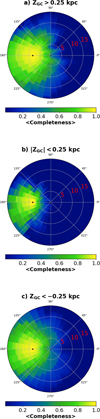 |
Fig. 20 Completeness for RC stars over the entire grid shown in galac-tocentric polar coordinates (ϕ, R) for three slices in ZGC above the plane (panel a), in the midplane (panel b), and below the plane (panel c). The concentric circles indicate bins in R, with values in kpc denoted in red. The black star indicates the Sun’s position. |
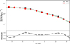 |
Fig. 21 Surface density of ɡdr3wise[RC] averaged over |ZGC| <1 kpc. Data are shown as black points, and the grey shaded area represents the two standard deviations over which each realisation of the data varies. The model predictions are shown in red and again the green shaded region represents the uncertainty in each bin. The residuals (1 -model/data) are shown in the lower panel. |
Best-fit parameters describing the Galactic disc.
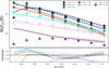 |
Fig. 22 Vertical counts as a function of |ZGC| at progressive annuli in R (2 kpc wide). In each case, the data are shown as stars, and the predictions from Model 2 as dashed lines in the same colour. The uncertainties in the best-fit model are represented by the shaded grey area. The residuals between data and model are shown in the lower panel. |
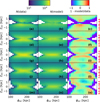 |
Fig. 23 Residuals between Model 2 from Table 4 and data in the projection, shown for the inner disc region (3 kpc < R < 10.5 kpc). In each row, the first column shows the number density of the data, the second row shows the number density predicted by the model, and the third row shows the residuals relative to the data. Each row represents a 1 kpc wide annulus in R. |
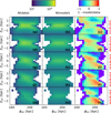 |
Fig. 24 Residuals between the model and data in the ϕ,ZGC projection. The setup is the same as Fig. 23 but for the outer disc (9.5 kpc<R< 14.5 kpc). |
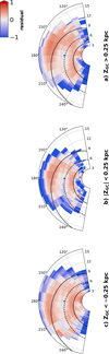 |
Fig. 25 Relative residual (1-model/data) for Model 2 from Table 4, applied to ɡdr3wise[RC], and shown in polar coordinates. The residuals are shown for three slices in ZGC above the plane (panel a), in the midplane (panel b), and below the plane (panel c). The two-arm NIR spiral model from Drimmel (2000) is overplotted as black curves. |
4.2.3 Testing warp parameters with real data
As discussed in the previous paragraphs, the best-fit of our assumed axisymmetric model exhibits diagonal residuals in the ϕ-ZGC projection. It is natural to wonder then whether the warp of the Milky Way can account for this outer feature.
To check this we tried to simultaneously fit for a model which included all the parameters from Model 2 (Table 4) as well as the additional four warp parameters (ϕw ,aw ,Rw ,hw0). However, the MCMC routine did not converge for these warp parameters, but interestingly, the remaining best-fit parameters did not significantly differ from Model 2. We then locked the best-fit parameters from Model 2, and only ran a fit for the four warp parameters, but again the MCMC had trouble converging. Our tests showed that the fit was in particular unable to constrain two parameters, aw, and ϕw which indicates the line-of-nodes (LON) for the warp. However, recent works have shown that the Milky Way’s warp does not have a constant LON, and that it curves towards lower ϕ beyond about R=12.5 kpc (Dehnen et al. 2023; Cabrera-Gadea et al. 2024; Jόnsson & McMillan 2024; Poggio et al. 2025). This could possibly explain in part why we are unable to constrain the ϕw as our warp parametrisation assumes a single LON for simplicity.
Figure 24 shows that the diagonal feature already starts appearing around R=9.5 kpc, i.e. well inside the regime where a constant LON is reasonable to assume. So, instead of adjusting all warp parameters simultaneously, we fit for only two (Rw, hw0), while keeping the other two fixed within the range of values found in the literature, at ϕw = (178°, 170°), and aw = (1.0, 2.0). Figure 26 shows the corner plots for four of these configurations, where we find Rw=8.25 kpc for (ϕw, aw)= (170°, 2.0), and Rw = 9.21 kpc for (ϕw, aw)= (178°, 1.5). Essentially, assuming that the LON of the warp varies between 2 to 10 degrees from the Galactic anti-centre allows us to place constraints on the onset of the warp at between 8.25 < Rw < 9.21 kpc. In Fig. H.1 we show the relative residuals in ϕ-ZGC: projection in the outer disc for these four configurations. Each column corresponds to one configuration, covering the 9.5 < R < 14.5 kpc part of the disc. Figure H.1 shows that, after having allowed for a warp, the residuals along the diagonal are much weaker. We summarise our best-fit warp parameters from this exercise in Table 5, where the uncertainties in hw0 & Rw are estimated by varying the Nmin,i between 50 and 20 as before for the Model 2.
Figure 27 shows different estimates of the warp amplitude available in the literature, together with the amplitude obtained with our sample, shown as a cyan shaded area for different assumed values of ϕw (between 170° and 178°) and aw (between 1 and 2). As we can see, for R ≳ 12 kpc the difference between the obtained warp amplitudes for different assumed aw and ϕw becomes prominent; however, the variation is still well below than 0.5 kpc at R ~ 14 kpc.
For R≲12 kpc, we note that our obtained warp amplitude is in broad agreement with the parametrisations by Uppal et al. (2024), based on RC stars, and in reasonable agreement with Cheng et al. (2020), based on general stellar populations in Gaia DR2/APOGEE, but larger than the estimate from Lόpez-Corredoira et al. (2002), again based on a selection of red clump stars. This latter estimate is in better agreement with the amplitude seen in the young giants (Poggio et al. 2025) and Cepheids (Chen et al. 2019). (See also other warp parametrisations based on Cepheids, e.g. Skowron et al. 2019; Dehnen et al. 2023; Cabrera-Gadea et al. 2024, whose estimated warp amplitudes are consistent with the Cepheid’s warp amplitude shown in Fig. 27.)
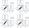 |
Fig. 26 Posterior probability distributions for two warp parameters (Rw,hw0) assuming Model 2 (Table 4) applied to ɡdr3wise[RC]. We show four cases where the other two warp parameters (ϕw,aw) have been fixed. The residuals for these are shown in Fig. H.1. |
Best-fit parameters describing the warp.
5 Discussion
Our best-fit model suggests that the RC stars are found in a two component disc (Table 4, Model 2), with a long (Rd ~ 4.24 kpc) and flaring disc (disc1) that is also potentially warped. This disc describes the stellar distribution from the Solar circle and beyond, while a second thicker and shorter (Rd~ 2.66 kpc) component that constitutes about 66% to the disc mass, describes well the distribution from 3 < R < 8 kpc. A natural question to ask then, is how our model compares with those of past works.
Scale length: There have been several studies mapping the scale parameters of the disc, and using a wide variety of tracers. Using flux maps in the near-infrared from the COBE satellite, Drimmel & Spergel (2001) found a scale length of about 2.31 kpc, which is close to what we find for the dominant component, possibly tracing the old thick disc.
Using high fidelity spectroscopic parameters from APOGEE, Lian et al. (2024) studied the surface density profiles of mono-abundance populations in the disc in bins of ages. They find that in the inner disc 3.5 < R < 7.5 kpc, the surface density profile is very flat, in agreement with high redshift Milky-Way type galaxies, while the region outside is best described by a single exponential with Rd = 2.6 kpc. For our sample, the measured surface density profile shown in Fig. 21 also shows a flatter profile inside of R < 7 kpc; however, this is in the observed data-space and so does not necessarily correspond to a flatter profile in the underlying model once selection effects are taken into account.
On the other hand, Binney & Vasiliev (2024, BV24), recently combined Gaia DR3 with chemistry from APOGEE–DR17, and distances from the StarHorse catalogue (Queiroz et al. 2023), to produce a chemodynamical model of the Galaxy using action-based distributions f(J). In their analysis they treat the Galaxy as a composite of several disc components, and in their Table 3 list the best-fit parameters for components of the Galactic disc, split by age. They provide Jϕ/υcirc(R0) = Rd, where Jϕ is the angular-momentum of stars. They find that the old disc has a scale length of about Rd=2.12 kpc, while the younger discs are at about Rd=4 kpc. Essentially, scale length was found to decrease with age. Without an age dissection, they find Rd=3.6 kpc, but this also includes the much older bulge component.
Our parameters are broadly in agreement with their analysis in that our model favours two components with long and short scale lengths respectively, and indeed our RC sample is expected to be populated by a mixture of ‘young’ and ‘old’ stars. In fact, the age distribution of the RC is not clearly determined. Using the APO-K2 asteroseismic catalogue, Warfield et al. (2024) recently derived the age of RGB stars, and showed that the RC in the traditional thin disc (α-poor) has a broad age distribution with a peak around 3–5 Gyr, while the age distribution of the RC in the traditional thick (α-rich) disc seems to be much flatter. This blurs the distinction between the old and young disc because, as they point out, the Galaxy seems to have many young α-rich RC stars that may have gained α-rich material through mass accretion in close binaries (Grisoni et al. 2024; Yu et al. 2024).
Vertical counts (scale height): In their best-fitting model, BV24 also provide the scale heights of the numerous disc components in terms of their vertical action as hɀ,⊙= 0.012 × Jɀ,0 (Binney & Vasiliev 2023). They find that their old disc has a scale height at the Sun of hɀ,⊙~ 0.28 kpc, while the high-α component has hɀ,⊙= 0.78 kpc. Interestingly, however, their young and the middle disc components have very short scale heights of hɀ,⊙~40 pc, suggesting that the youngest populations in the Milky Way are confined to a very thin sheet-like distribution. Therefore, though our ‘thin’-flaring disc may not be as young as the young counterpart of BV24, that it has a short scale height at the Sun is perhaps not too surprising. Meanwhile the thicker disc component in our RC sample has hɀ,⊙ = 0.48 kpc, and this could be due to some overlap with both the old and high-α component of BV24. Indeed, using extremely precise stellar parameters from Gaia DR3 (GSP-Spec), Recio-Blanco et al. (2024) showed the presence of a bimodality in the RC on the Kiel diagram, that is suggested to map to the typical bimodality seen in [α/Fe]–[Fe/H] separating the traditional thin and thick disc. However, due to the flare, our ‘thin’ disc with a longer scale length has a larger scale height than the second ‘thick’ disc which has a larger scale height at the Sun. Indeed, the traditional distinction of the two disks as ‘thin’ and ‘thick’ is misleading. (For further discussion see Bland-Hawthorn et al. 2019).
The vertical counts in the RC disc are generally well traced by the parameters of our Model 2 with two discs, as shown in Fig. 22. In the observed counts (starred points) the flare is seen as a change in slope of N(ɀ|R) as a function of |ZGC|. Specifically, we find log10 Rfl [kpc] ~ 0.36 for the flared disc component. Figure 28 shows the predicted profile of the scale height as a function of R, shown as black curves for both the single disc (Model 1, dashed curve) and disc1 of Model 2 (solid curve). Also plotted are a few profiles of the scale height from the literature: Lόpez-Corredoira et al. (2002, LC02 hereafter) studied the disc in the NIR using data from 2MASS where the sample is dominated by RC-like stars. They found the normalisation hɀ,⊙= 0.31 kpc, and a flare parameter of 1og10 Rfl= 0.53 (blue curve). More recently, combining both 2MASS and Gaia, Uppal et al. (2024, U24 hereafter) also constructed an all-sky RC sample and found hɀ,⊙= 0.35 kpc, but a weaker flare parameter of 1og10 Rfl= 0.85 (red curve). Cantat-Gaudin et al. (2024, TCG24 hereafter) fit for density profiles of a combined Gaia–APOGEE sample of low [α/Fe] RC stars for which high quality spec-troscopic parameters are available. This allowed them to study the profiles by population, specifically by metallicity. Crucially, their model fitting takes into account the complex selection function of the combined sample. In the range −0.3 <[Fe/H]< 0.4, where we expect most of our RC stars to be populated, they find 0.24 < hɀ,⊙ < 0.31 kpc with the flare ranging between 0.64 < 1og10 Rfl < 1.09. In Fig. 28 we include the results from TCG24 as a shaded grey region, showing the span of the flare parameter between −0.3< [Fe/H] <0.3. Except for U24, all studies use an exponential parameterisation for the flare similar to us. However, all the aforementioned studies only consider a single disc component in their fitting procedure.
Our single disc model (Model 1) in Table 4 for just a single disc component predicts hɀ,⊙= 0.46 kpc and log10 Rfl= 2.14, and we have over plotted this in Fig. 28 as a dashed black curve. It is interesting to note that between 8<R<11 kpc, the profile is very similar to that found by U24, and also quite similar to the single exponential discs of TCG24, but offset in the scale height. However, as noted earlier, this single disc model is unable to account for the stellar counts in the outer disc.
Our value of log10 Rfl= 0.36 for the flare is smaller than the aforementioned studies, which would indicate a stronger flare than previously found, though looking at Fig. 28, the profile is not too dissimilar to that found by LC22, except we have a smaller normalisation of hɀ,⊙= 0.18 kpc. However, we note that our model up to this point does not account for the warp, which the model might be compensating for with a stronger flare.
Warp: As discussed in Sect. 4.2.3, we see a clear signature of the warp in the outer disc residuals (Fig. 24), which we attempted to add to our model. While the resulting warp amplitude suggests that it may differ between young and old populations (Fig. 27), we should bear in mind that, in this study at least, we are able to explore the warp only over a limited portion of the Galactic disc, while the warp is a large-scale feature, and we therefore should avoid over-interpreting the warp amplitude obtained here. In any case, Fig. 27 shows that our knowledge of the warp amplitude is quite uncertain, especially for the old populations. Moreover, we note that while the residuals in the outer disc (shown in Fig. H.1) are lower than those in the non-warped case, they do not disappear completely. This may be due in part to assuming an over-simplified warp geometry with a straight line of nodes. whereas the young populations clearly show the line-of-nodes remains straight only for R ≃ 12 kpc (Dehnen et al. 2023; Poggio et al. 2025). Nevertheless, our tests represent a first step in the right direction, confirming the warp signature in our RC sample, but there is still need for further exploration in future work.
Two-armed spiral: In the previous section we also discussed the residuals between the two-disc model and the data projected on the Galactic plane (Fig. 25), noting that they seem to show evidence of a two-arm spiral pattern with geometry similar to that inferred from NIR data (D00). In Fig. 29 we show the residuals for |ZGC| < 1kpc also with the geometry of spiral arm models based on masers (Reid et al. 2019, hereafter R19) and the Cepheids (Drimmel et al. 2025). We find that the location of the outer residuals also roughly coincides with the location of the Outer Arm proposed by R19. The Perseus arm as mapped by the Cepheids and the HI (Levine et al. 2006) also cross this region, though with an apparently higher pitch angle. Recently Uppal et al. (2023) also claim to have detected the Outer Arm in a sample of RC stars selected using Gaia and 2MASS photometry using the overdensity mapping technique of Poggio et al. (2021). However, we note that the arm detected here in the RC residuals is much broader than the one they report. This is likely due to their choice of bandwidths for calculating the overdensity, restricting their sensitivity to features with scale lengths between 0.3 and 2 kpc. In addition, the overdensity mapping approach may be highlighting a small fraction of young stars transiting in their selected RC region of the colour-magnitude diagram as they evolve from the main sequence to the giant branch. Finally, though we note generally higher residuals in the first quadrant between 6 < R < 8 kpc from 130° < ϕ < 160°, we do not detect a feature in the residuals that might correspond to the Local arm, especially near the disc midplane (|ZGC| < 0.25 kpc, see middle panel of Fig. 25), where the Local arm instead falls in an under-dense portion of the disc that lies along the expected inter-arm region of the NIR arms. This is in contrast with Lin et al. (2022), who also use the overdensity mapping approach for a selection of RC stars, and may suffer the same contamination issues mentioned above.
In summary, if our residuals are mapping a spiral perturbation in the old stellar population, the geometry and profile of this perturbation is more consistent with a broad two-armed spiral than the multiple arms traced by young populations and star formation products (R19; Zari et al. 2021; Poggio et al. 2021, Gaia23). However, we should bear in mind that the residuals shown in Fig. 25 might also be influenced by additional effects. For instance, any deviation of our best-fit parametrisation (especially in the case of two or more disc-like components) with respect to the unknown true underlying density distribution might result in radial over/under-densities, which might interfere with interpreting any possible spiral arm signature. In addition, our residuals are with respect to our model without a warp, which may introduce additional residuals in the outer disc.
Nevertheless, that the geometry and width of the spirals as traced by the RC stars might not be the same as that seen in the young populations should not be a surprise. Presumably the RC population is tracing the old, kinematically relaxed stellar population that dominates the underlying mass distribution of the stellar disc, while young stars are a product of the response of the gas to a disc with multiple pattern speeds and, possibly, external perturbations (Purcell et al. 2011; Pettitt et al. 2016). If the residuals from our axisymmetric disc model are tracing a spiral perturbation in the old stellar disc of the Milky Way, their magnitude suggests that this perturbation is at the level of 10–20%. These residuals in the outer disc extend to a galactocentric radius of at least 14–15 kpc, well beyond the outer Lindblad radius of the bar which is at a radius of 10–12 kpc based on recent estimates of the bar’s pattern speed (Binney 2020; Chiba & Schönrich 2021; Dillamore et al. 2024; Lucchini et al. 2024, Gaia23), so that any spiral perturbation responsible for these residuals must have a lower pattern speed than the bar, as a spiral arm perturbation is expected to be located between its own inner and outer Lindblad resonances.
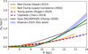 |
Fig. 27 Comparison between the warp amplitude obtained in this work and other parametrisations available in literature based on different stellar tracers. The blue shaded area shows the warp amplitude obtained in this work in the region where our dataset and our adopted approach allow us to reasonably constrain the warp shape. At larger galactocentric radii (R ≳ 12 kpc, grey shaded area), it is not possible for our approach to give a reliable estimate of the warp amplitude based on our dataset due the lack of convergence of the fitting routine (see discussion in the text). |
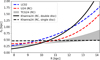 |
Fig. 28 Profile of scale height as a function of R predicted from our best-fit model with two discs (Model 2) for ɡdr3wise[RC], shown as a black solid curve (disc1), and for the single disc model (Model 1), shown as a dashed black curve. The red and blue dashed curves and grey shaded area show the profiles from other studies of RC stars in the literature. (See text for further details.) |
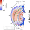 |
Fig. 29 Same as Fig. 25 but for the |ZGC| <1 kpc slice. Various spiral arm models are overplotted: Coloured dashed lines show model based on masers from Reid et al. (2019), coloured solid lines show model based on Cepheids (Skowron et al. 2025; Drimmel et al. 2025), and in black is the two-arm NIR model from D00. |
6 Summary
In this paper, we have constructed an all-sky catalogue of RC candidates for which we could derive reliable distances using MIR photometry from AllWISE. This sample of nearly ten million stars allowed us to map the stellar number density for galactocentric radii between 3 < R [kpc] < 14 and at a distance from the Galactic mid-plane of |ZGC | < 2 kpc. Taking advantage of the near Gaussian luminosity function of the RC and 3D extinction maps, we built a selection function tailored to our sample, i.e. the probability of observing an RC star at a given location on the sky at a given magnitude. The selection function then allowed us to build a three-dimensional completeness map of our sample and to fit a range of models to the observed stellar density. It is only by taking into account the selection function that we can use the RC sample to trace a large fraction of the Galactic disc. Indeed, limiting ourselves to a sample with 90% completeness would limit our volume to within only 2–4 kpc of the Sun (see Fig. 20).
Our best model consists of two discs, where each is exponential both radially and vertically. Specifically, the RC population of the Galaxy seems to be well described by a long and flared disc component that makes up about 36% of the stellar mass. It has a scale length of Rd = 4.24 kpc and scale height at the Sun of hɀ,⊙ = 0.18 kpc, flaring to 2 kpc at R = 14 kpc. The remaining 66% of the mass is in a disc with a scale length of Rd = 2.66 kpc and a scale height of hɀ2,⊙ = 0.48 kpc without a flare. So, while our model is purely geometrical, it is interesting that our two-component disc model recovers two disc components similar to those seen when mapping the [α/Fe] distribution as a function of R and ɀ, namely, a disc with a short scale length and thicker scale height dominating the inner Galaxy and a second flaring disc with a longer scale length dominating the outer Galactic disc (Hayden et al. 2015). This suggests that while we have not made a chemical separation of our RC sample, we apparently recover the same two-disc morphology as evidenced in the [α/Fe] distribution.
By subtracting the best-fit model from the data, we found residuals in both the inner and the outer disc. These residuals show a clear warp signature beyond R > 10 kpc, and in the Galactic plane, they show a signature that seems to coincide with the expected location of the spiral arms inferred from the NIR (D00; Drimmel & Spergel 2001; Benjamin et al. 2005; Hou & Han 2015), corroborating the two-armed geometry implied by the observed spiral arm tangents at these wavelengths and implying a perturbation in the mass surface density of 10–20%. Confirming these results will require better modelling of the outer disc to fully take into account the warp and/or a deeper catalogue towards the inner Galaxy, where extinction still limits the volume we are able to sample.
We have modelled the density of the RC stars with a purely geometrical model, which requires sufficient knowledge of the extinction in three dimensions as well as the combined selection function of the photometric surveys used. Because of these stringent conditions for mapping the three-dimensional density in the Galactic plane, earlier attempts to verify the existence of a spiral perturbation in the mass density of the stellar disc have relied on the measured velocities of tracers (Grosbøl & Carraro 2018; Eilers et al. 2020). Recently, Palicio et al. (2023) detected spiral-like features in the radial action, JR, of disc stars. However, since Gaia DR3 it has become clear that the bar of the Milky Way dominates the velocity field of the disc well beyond co-rotation (Gaia23), thus complicating any possible interpretation of the disc’s velocity field. Nevertheless, we intend to study the velocities of the RC sample in the future. Indeed, including this additional information may allow us to better constrain the warp in this old stellar population.
Data availability
The RC catalogue corresponding to Fig. 9, is available at the CDS via https://cdsarc.cds.unistra.fr/viz-bin/cat/J/A+A/701/A270.
Acknowledgements
We thank the anonymous referee for their constructive comments. SK & RD acknowledge support from the European Union’s Horizon 2020 research and innovation program under the GaiaUnlimited project (grant agreement No 101004110). SK acknowledges use of the INAF PLEIADI@IRA computing resources, and would like to thank Hai-Feng Wang & Paul McMillan for useful suggestions. RD & EP are supported in part by the Italian Space Agency (ASI) through contract 2018-24-HH.0 and its addendum 2018-24-HH.1-2022 to the National Institute for Astrophysics (INAF). We also thank Kevin Jardine for visualisation of the selection function. This work presents results from the European Space Agency (ESA) space mission Gaia. Gaia data are being processed by the Gaia Data Processing and Analysis Consortium (DPAC). Funding for the DPAC is provided by national institutions, in particular the institutions participating in the Gaia MultiLateral Agreement (MLA). The Gaia mission website is https://www.cosmos.esa.int/gaia. The Gaia archive website is https://archives.esac.esa.int/gaia. This work made use of the https://gaia- kepler.fun crossmatch database created by Megan Bedell. This work has used the following additional software products: TOPCAT, and STILTS (Taylor 2005); Matplotlib (Hunter 2007); IPython (Pérez & Granger 2007); Pandas (The pandas development team 2020); Astropy, a community-developed core Python package for Astronomy (Astropy Collaboration 2018); NumPy (Harris et al. 2020); Vaex (Breddels & Veljanoski 2018); and SpiralMap (Prusty & Khanna 2025).
Appendix A Intrinsic correlation plot
For the sample of stars from ɡdr3wise where σϖ/ϖ < 0.05, we can infer their absolute magnitudes from their inverse parallax distances (dϖ′). Retaining those with inferred absolute magnitudes within 1σ values from literature, we can assume these are consistent with being on the red clump phase. To these stars then, we assign an absolute magnitude from the Gaussian  , and using dϖ′, can predict their apparent magnitudes in both passbands (GRC, W1RC). Figure A.1 shows the distribution of difference between the true and predicted apparent magnitudes, for which we find the Pearson correlation coefficient ~0.42.
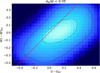 |
Fig. A.1 Intrinsic correlation between the G and W1 bands for RC stars with σϖ/ϖ < 0.05. The (1,2)σ contours of this distribution are marked in black, the red dotted line is the 1:1 relation, while the Pearson correlation coefficient for this set is 0.43. |
Appendix B Distance posterior PDF from CBJ21
For clarity, we reproduce here the relations to obtain the posterior PDF from CBJ21. The geometric distance prior is written in the form of a generalised gamma distribution,
 (B.1)
(B.1)
valid for distance, r ≥ 0. Given a HEALpixel (level 5), hpix, one can obtain the parameters α, β, and L from the auxiliary file provided by CBJ21. Then, using the likelihood function,
 (B.2)
(B.2)
where ϖ′ = ϖ + 0.017, we can write the posterior PDF as a product of the likelihood and the prior as
 (B.3)
(B.3)
Appendix C RC validation
C.1 Selecting red clump from stellar parameters
In this paper, our ɡdr3wise [RC] sample is selected by combining Gaia astrometry & photometry with AllWISE photometry. Ultimately, however, a purer sample of RC stars can be selected using spectroscopic stellar parameters (log ɡ, [Fe/H], Teff). In K19, we had developed such a scheme to select high fidelity RC stars, and we provide a short summary of this below:
![Mathematical equation: $1.8 \le \log \,g\, \le \,0.0018\,{\rm{dex}}\,{{\rm{K}}^{ - 1}}\left( {{T_{{\rm{eff}}}} - {T_{{\rm{eff}}}}^{{\rm{ref}}}\left( {\left[ {{\rm{Fe}}/{\rm{H}}} \right]} \right)} \right) + 2.5,$](/articles/aa/full_html/2025/09/aa52798-24/aa52798-24-eq60.png) (C.1)
(C.1)
![Mathematical equation: $Z < 1.21{\left[ {{{\left( {J - K} \right)}_0} - 0.05} \right]^9} + 0.0011,$](/articles/aa/full_html/2025/09/aa52798-24/aa52798-24-eq61.png) (C.2)
(C.2)
![Mathematical equation: $Z < {\rm{Min}}\left( {2.58{{\left[ {{{\left( {J - K} \right)}_0} - 0.40} \right]}^3} + 0.0034,\,0.06} \right),$](/articles/aa/full_html/2025/09/aa52798-24/aa52798-24-eq62.png) (C.3)
(C.3)
 (C.4)
(C.4)
where
![Mathematical equation: ${T_{{\rm{eff}}}}^{{\rm{ref}}}\left( {\left[ {{\rm{Fe}}/{\rm{H}}} \right]} \right) = - 382.5\,{\rm{K}}\,{\rm{de}}{{\rm{x}}^{ - 1}}\left[ {{\rm{Fe}}/{\rm{H}}} \right] + 4607\,{\rm{K}}$](/articles/aa/full_html/2025/09/aa52798-24/aa52798-24-eq64.png) (C.5)
(C.5)
and Z = Z⊙10[Fe/H], with Z⊙ = 0.019. Here, (J – K)0 is the intrinsic colour in 2MASS passbands for RC stars. One can derive the intrinsic colour solely from stellar parameters as
 (C.6)
(C.6)
where X =[Fe/H] and Y = 5040 K/Teff, and the coefficients as listed in Table C.1.
A23: In this paper, we only use the relations above for validation. In particular, we select RC candidates from the recently published stellar parameter catalogue of Andrae et al. (2023)(A23) who derived these for Gaia stars with XP spectra and AllWISE photometry (about 125 million in all). We are able to select 6, 840, 662 RC-like stars from their catalogue, and find that 63% of these are present in ɡdr3wise[RC]. Figure C.1 shows the CMD in both Gaia and AllWISE colours for the ɡdr3wise parent sample in grey, with the ɡdr3wise[RC] shown as red contours and the sample selected from A23 in blue contours. In Fig. C.2 we use the distance priors from CBJ21 to show the CaMD for these in both Gaia and AllWISE colours, with the two RC samples once again indicated by red and blue contours. Our photo-astrometrically selected RC and that spectroscopically selected from A23 trace very similar distributions in these figures, though our selection is a bit more conservative, covering a smaller area in (log ɡ, Teff) space.
APOGEE and GALAH: Next we consider the two main contemporary high resolution spectroscopic surveys APOGEE (Abdurro’uf et al. 2022, DR17) and GALAH (Buder et al. 2021, DR3). For each, we use their internal crossmatches to Gaia EDR3 source_id. We find about 150,000 of our RC sources in common with the two surveys combined. The Kiel diagram for APOGEE & GALAH surveys is shown in Fig. C.3, with our RC selection overlaid as contours at (1,2)σ, which lie within 1.8< log ɡ <3.0. Interestingly, in both comparisons, we also note the presence of an overdensity around (Teff, log ɡ)= (5100 K, 2.9). This would be the secondary red clump population, which are more massive and younger counterparts to the typical RC, burning helium in their cores after leaving the RGB without having experienced a helium flash (Girardi 2016).
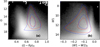 |
Fig. C.1 Colour magnitude diagram for the ɡdr3wise parent catalogue shown for Gaia and AllWISE colours. In each panel, we indicate the selected RC sample using the red contours (1σ, 2σ). Also, shown in blue contours are the spectroscopically selected RC from A23. |
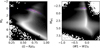 |
Fig. C.2 Colour-absolute magnitude diagram for the ɡdr3wise dataset, with MG vs (G – GRP)0 shown in panel (a), and MW1 vs (W1 – W2)0 shown in panel (b). The red contours in each panel represent the selected ɡdr3wise[RC] stars. Also, shown in blue contours are the spectroscopically selected RC from A23. |
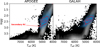 |
Fig. C.3 External validation of ɡdr3wise[RC] against the spectroscopic catalogues, APOGEE (panel a) and GALAH (panel b). For each survey we show the overall Kiel diagram, with the common sources in our catalogue overplotted (blue points). Also, shown is the (1,2)σ density contours for the common sources. Note: the presence of an overdensity around (Teff, log ɡ)= (5100 K, 2.9), which is likely the secondary red clump population. |
C.2 Selecting RC in Galaxia and metallicity CDF
In order to look at properties of RC stars, we generated an all-sky mock catalogue with magnitude limit of G <17.5, using the Galaxia population synthesis code (Sharma et al. 2011), which implements the Besancon Galaxy model (Robin et al. 2003). The warpflare option was set to 1. Galaxia allows for sampling of stars in a continuous fashion across the sky, and also provides photometry, in most of the commonly used bands. From the mock, we selected RC stars using the scheme laid out in Sect. C.1. Additionally, we select only those stars that have an initial stellar mass greater than their RGB tipping mass, and that are present in the Galactic disc. The CaMD in both Gaia and AllWISE colours is shown in Fig. 3, with the RC population indicated as black contours. For this sample, the Cumulative Distribution Function (CDF) of their metallicity in Fig. C.4 for three cuts in stellar age at τ=(5,7,10) Gyr is shown in Fig. C.4, where we see that in general the fraction of stars with [Fe/H]<− 0.4 ranges around 15–20% for the typical ages of RC stars (τ <5 Gyr). For completion, Fig. C.4 also shows the metallicity CDF of RC that we select from A23 (purple curve), and this is consistent with that seen in Galaxia.
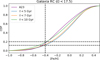 |
Fig. C.4 Cumulative distribution function (CDF) of the metallicity of RC population selected from Galaxia for a magnitude limited survey at G < 17.5. Three CDF curves are shown, each for a cut in maximum stellar age at τ=(5,7,10) Gyr. The horizontal black lines indicate CDF=(0.12,0.2), while the vertical black line indicates [Fe/H]=−0.4. Also shown is the CDF for the spectroscopically selected RC from A23. |
C.3 Comparison with asteroseismology
In general the selection scheme laid out in Sect. C.1 should be able to select high fidelity RC stars. However, given the close overlap with the RGB and secondary RC populations in both photometric and spectroscopic spaces, it is easy to also select contaminants. The gold-standard for distinguishing between these phases of stars is asteroseismology - the study of stellar oscillations. This technique is sensitive to the internal structure of stars and thus allows one to select pure RC stars. In red giant stars, these oscillations are excited by near-surface convection, and are broadly characterised as two dominant modes: a) acoustic (p-mode): the propagation zone of such modes is the outer envelope of the star, with pressure acting as the restoring force. Observationally, these modes are approximately equally spaced in oscillation frequency; b) gravity (ɡ-mode): such modes propagate in the interior of the core, and buoyancy acts as the restoring force here. Pure ɡ-modes are approximately equally spaced in their period. In evolved stars, coupling between the p and ɡ modes results in the so called mixed modes. In their seminal work, Bedding et al. (2011) showed that such mixed modes in red giant stars can help distinguish between the RGB and the RC phases.
This relies on their different distributions in the ∆ν-∆P plane. Here, ∆ν is the frequency separation between adjacent p-modes with the same angular degree but at different radial order, while ∆P is the period spacing between adjacent mixed modes. Fundamentally, this is due to the differences in the structure of the cores of the two types. While, RGB have a radiative core, RC stars have a fully convective core. It turns out that mixed modes cannot stably propagate though convective cores, but can do so in the radiative regions above the core in RC stars. Since, the radiative region in RC stars is smaller compared to RGB stars, this has the consequence of larger PS, thus making it a key discriminant between the two stellar phases (Hekker & Christensen-Dalsgaard 2017). We now compare our sample to three independent publicly available catalogues that use asteroseismology to classify stellar phases. For each of the following, we provide the precision, recall and accuracy, as quality markers, defined as Precision = (True positive/Results), Recall = (True positive/ True positive + False Negative), and Accuracy = (True positive + True Negative) / (Total - Unclassified).
Yu et al. (2018, Yu18 hereafter) carried out an extensive asteroseismic analysis on a sample of 16,094 red giants with light curves from the Kepler Space Telescope (Borucki et al. 2010; Koch et al. 2010). In addition to global seismic parameters, their catalogue also provides a classification for the stellar phase, given as [0:‘unclassified’ (706), 1: RGB (7685), 2: RC (7703)], with the number of each quoted in bold. We make use of the 1 arcsec spatial crossmatch performed for Kepler8 stars with Gaia DR3 in order to grab the Gaia source identifier (ID) for the Yu18 sample. We find 8327 stars in common between our catalogue and Yu18, out of which 78% were classified as phase 2 by the latter. Taking into account the ‘impurity’ (RGB) in our sample, with respect to Yu18, our selection achieves an accuracy of about 80%.
In the literature, one finds a diverse range of techniques employed in the classification of the stellar phase of oscillating giants, and the results are also varied. Elsworth et al. (2019, Els19 hereafter) compiled a ‘consensus’ evolutionary state for 6000 red giant stars, from four different methods of analysing the frequency-power spectrum. This sample has been observed by Kepler, and also by the APOGEE and/or SDSS surveys. In their catalogue, they assign the following primary classifications, ’RGB’ (red giant branch), ’RC’ (red clump), ’2CL’ (secondary red clump), ’AGB’ (asymptotic giant branch), and, ’U’ (unclassified). Additionally, some stars are assigned a combination of these classifications, i.e. ’2CL/U’, ’AGB/U’, ’RC/2CL’, ’RC/U’, ’RGB/AGB’, ’RGB/U’. We obtain the Gaia EDR3 source IDs for Els19, following the exact same crossmatching procedure as we did for Yu18. Next, we select three populations, namely, a) RC: where ’consensus’==’RC’|’RC/2CL’|’RC/U’|’2CL’|’2CL/U’, b) RGB: where ’consensus’ ==’AGB/U’|’RGB’|’RGB/AGB’|’RGB/U’|’U’, and, c) Unclassified: where consensus==’U’. We find 3047 stars in common with Els19, out of which, 72% are classified as RC by the latter. Taking into account the impurity (RGB), we still achieve an accuracy of about 83%, though we of course note the lower completeness compared to Yu18.
Lucey et al. (2020, L20 hereafter) put out a photometric catalogue of 2.6 million RC candidates. Their method involves predicting asteroseismic parameters (PS, ∆ν) and stellar parameters (loɡɡ, Teff ) from spectral energy distributions (SED), using a neural network trained on RC stars from Ting et al. (2018). They combined photometry from Pan-STARRS, All-WISE, 2MASS, and Gaia DR2. In their catalogue, they provide two sets of RC samples: a) ’Tier 2’: 2,210,769 candidates with a contamination rate of ≈ 33%, and b) ‘Tier 1’: A superior set of 405,231, with a lower contamination rate of ≈ 20%. For our comparison we restrict to their stricter ‘Tier 1’ sample. As before, we make use of the gaiaedr3.dr2_neighbourhood table to recover the corresponding Gaia EDR3 source IDS for all stars in the L20 catalogue. In Fig. C.5, we illustrate the comparison between ɡdr3wise [RC] and L20 on the Kiel diagram, using stellar parameters from the latter. In Fig. C.5(a) we show all the red clump candidates (Tier 1 and Tier 2), from L20, and the 1,2, and 3 σ density contours are shown in black. Also, marked are typical crude boundaries, 1.8< log ɡ <3.0, used to select RC, shown as a guide to the reader. We noticed the presence of a skew in the density distribution at lower log g values beyond the lower end of this crude boundary. Next, in Fig. C.5(b), we show the stars in common between L20 and ɡdr3wise [RC], where we note that the common selection lies well within the crude boundary and in a tight locus in log ɡ. It is quite clear that our selection is a bit more conservative, and at the cost of accuracy, we miss out on possible contaminants in the L20 catalogue. Finally, in Fig. C.5(c), we plot those stars which are classified as ’nan’ in L20, but are present in our selection scheme. It is interesting to note that the stellar parameters for these from L20 are consistent with these being part of the red clump, although there are possible contaminants present, especially in the region with log ɡ>3 and Teff>5000 K. Since our selection method relies on both updated astrometry and photometry from Gaia EDR3, as well as AllWISE, we are fairly confident that a large fraction of these are consistent with being members of the RC.
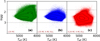 |
Fig. C.5 External validation of our catalogue (RC-ALL here) by cross-matching against the catalogue of L20, shown on the Kiel diagram using parameters from the latter. We also overplot density contours at (1,2,3)σ, shown in black. The typical crude boundary for RC stars, 1.8< loɡɡ <3.0 is indicated by black dotted lines. Panel (a) shows that the distribution of L20 falls mostly (1,2 σ) inside the crude boundaries, and is also broad in Teff. Panel (b) shows the crossmatch between L20 and our sample. Nearly all of these overlapping sources lie between the crude boundary, and also display a tighter distribution in log ɡ. Panel (c), finally shows the stars that are present in L20, and are not classified as RC, but are present in our sample. Again, the stellar parameters from L20 for those that lie within the (1,2)σ contour are consistent with expected boundaries, although there are possible contaminants around the region log ɡ>3 and Teff>5000 K. |
Appendix D Sub-selection function queries: Gaia X AllWISE
To build the sub-selection function layer of the selection function, we compute the ratio of sources that end up in the ɡdr3wise crossmatch versus all sources in Gaia. We compute this ratio as a function of sky position (at HEALPix level 5), and G (1 magnitude wide bins). To this end, we ran the following query on the Gaia archive:
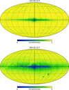 |
Fig. D.1 Completeness map for the sub-selection layer for ɡdr3wise dataset at HEALPix level 5, shown for a bright (top) and a faint magnitude bin (bottom). |
In Fig. D.1 we show the on sky projection of this sub-selection function for two magnitude bins, one at the bright end (12< G <13) where most of the sky has a high degree of completeness (though with noise due to small number statistics), and another at the faint end (16< G <17) where it is much less so. The reduced completeness near the Galactic plane and towards the inner Galaxy, as well as towards the Large and Small Magellanic Clouds, is mainly due to crowding and the low resolution of AllWISE.
Appendix E Corner plots for mock cases
We show here the corner plots of the MCMC fit (1000 iterations) carried out on the two mock cases described in Sect. 4.1. In case I we demonstrate the fit on an exponential disc with scale height Rd, scale length hɀ,⊙, and a flare scale length Rfl (Fig. E.1). In case II, we generate a mock galaxy identical to that in case I, except that it is also forced to be warped, and is described by four additional parameters (ϕw,Rw,hw0,aw) as shown in Fig. E.2.
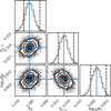 |
Fig. E.1 Mock case I: Corner plots from the MCMC fitting for the three parameters describing mock case I, with the best-fitting values indicated as vertical lines. The true values for this example are: Rd = 3.3 kpc, hɀ,⊙ = 0.3 kpc, log10 Rfl = 0.6. |
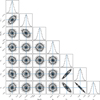 |
Fig. E.2 Mock case II: Corner plots from the mcmc fitting for the three parameters describing mock case I, with the best-fitting values indicated with blue lines. The true values in this example are: Rd = 3.3 kpc, hɀ,⊙ = 0.3 kpc, loɡ10 Rfl = 0.6, ϕw = 170°, Rw = 6.5 kpc, aw = 1.0, hw0 = 0.3 kpc. |
Appendix F Corner plot: Single disc fit
Figure F.2 shows the corner plot for the fit to the ɡdr3wise[RC] dataset, for the case assuming only one disc component. Here we fit for the scale length, scale height and flare parameter only (see Model 1 in Table 4). The residuals for this fit are shown in Fig. F.1 in ϕ-ZGC projection for the inner (3<R<10.5 kpc) and the outer disc regions (9.5<R<14.5 kpc). Compared to the residuals for the double disc case shown in Fig. 23, & Fig. 24, this model does not fit the disc well across all R, and is especially problematic in the outer disc region.
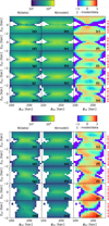 |
Fig. F.1 Residuals between the model and data in the ϕ,ZGC projection. The setup is the same as Fig. 23 for the inner disc and Fig. 24 for the outer disc, but it is for Model 1, which allows for only a single disc component (Table 4). |
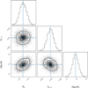 |
Fig. F.2 Posterior probability distributions for Model 1(Table 4) applied to ɡdr3wise[RC]. This model allows for only one disc component. |
Appendix G Corner plot: Double disc fit
Fig. G.1 shows the corner plot for fit to the ɡdr3wise[RC] dataset, assuming a double disc model. Here we fit for the scale length, scale height of two independent exponential discs, with one of these allowed to flare (see Model 2 in Table 4). We do not fit for the warp in this model.
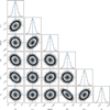 |
Fig. G.1 Posterior probability distributions for Model 2 (Table 4) applied to ɡdr3wise[RC]. This model allows for two discs. |
Appendix H Warp fitting
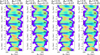 |
Fig. H.1 Relative residual (1-model/data) for ɡdr3wise[RC], corresponding to the four cases exploring warp parameters shown in Fig. 26. For each case, we show the residuals in successive R annuli (9.5 kpc<R< 14.5 kpc). The corner plots corresponding to each case are shown in Fig. 26. |
References
- Abdurro’uf, Accetta, K., Aerts, C., et al. 2022, ApJS, 259, 35 [NASA ADS] [CrossRef] [Google Scholar]
- Andrae, R., Rix, H.-W., & Chandra, V. 2023, ApJS, 267, 8 [NASA ADS] [CrossRef] [Google Scholar]
- Astropy Collaboration (Price-Whelan, A. M., et al.) 2018, AJ, 156, 123 [Google Scholar]
- Aumer, M., & Binney, J. 2017, MNRAS, 470, 2113 [NASA ADS] [CrossRef] [Google Scholar]
- Bailer-Jones, C. A. L. 2015, PASP, 127, 994 [Google Scholar]
- Bailer-Jones, C. A. L., Rybizki, J., Fouesneau, M., Demleitner, M., & Andrae, R. 2021, AJ, 161, 147 [Google Scholar]
- Bedding, T. R., Mosser, B., Huber, D., et al. 2011, Nature, 471, 608 [Google Scholar]
- Benjamin, R. A., Churchwell, E., Babler, B. L., et al. 2005, ApJ, 630, L149 [NASA ADS] [CrossRef] [Google Scholar]
- Bennett, M., & Bovy, J. 2019, MNRAS, 482, 1417 [NASA ADS] [CrossRef] [Google Scholar]
- Binney, J. 2020, MNRAS, 495, 895 [NASA ADS] [CrossRef] [Google Scholar]
- Binney, J., & Vasiliev, E. 2023, MNRAS, 520, 1832 [NASA ADS] [CrossRef] [Google Scholar]
- Binney, J., & Vasiliev, E. 2024, MNRAS, 527, 1915 [Google Scholar]
- Bland-Hawthorn, J., & Gerhard, O. 2016, ARA&A, 54, 529 [Google Scholar]
- Bland-Hawthorn, J., Sharma, S., Tepper-Garcia, T., et al. 2019, MNRAS, 486, 1167 [NASA ADS] [CrossRef] [Google Scholar]
- Borucki, W. J., Koch, D., Basri, G., et al. 2010, Science, 327, 977 [Google Scholar]
- Bovy, J., Bird, J. C., García Pérez, A. E., et al. 2015, ApJ, 800, 83 [NASA ADS] [CrossRef] [Google Scholar]
- Bovy, J., Rix, H.-W., Schlafly, E. F., et al. 2016, ApJ, 823, 30 [NASA ADS] [CrossRef] [Google Scholar]
- Breddels, M. A., & Veljanoski, J. 2018, A&A, 618, A13 [NASA ADS] [CrossRef] [EDP Sciences] [Google Scholar]
- Buder, S., Sharma, S., Kos, J., et al. 2021, MNRAS, 506, 150 [NASA ADS] [CrossRef] [Google Scholar]
- Cabrera-Gadea, M., Mateu, C., Ramos, P., et al. 2024, MNRAS, 528, 4409 [NASA ADS] [CrossRef] [Google Scholar]
- Cannon, R. D. 1970, MNRAS, 150, 111 [NASA ADS] [CrossRef] [Google Scholar]
- Cantat-Gaudin, T., Fouesneau, M., Rix, H.-W., et al. 2023, A&A, 669, A55 [NASA ADS] [CrossRef] [EDP Sciences] [Google Scholar]
- Cantat-Gaudin, T., Fouesneau, M., Rix, H.-W., et al. 2024, A&A, 683, A128 [NASA ADS] [CrossRef] [EDP Sciences] [Google Scholar]
- Castro-Ginard, A., Brown, A. G. A., Kostrzewa-Rutkowska, Z., et al. 2023, A&A, 677, A37 [NASA ADS] [CrossRef] [EDP Sciences] [Google Scholar]
- Chen, X., Wang, S., Deng, L., et al. 2019, Nat. Astron., 3, 320 [NASA ADS] [CrossRef] [Google Scholar]
- Cheng, X., Anguiano, B., Majewski, S. R., et al. 2020, ApJ, 905, 49 [Google Scholar]
- Chiba, R., & Schönrich, R. 2021, MNRAS, 505, 2412 [NASA ADS] [CrossRef] [Google Scholar]
- De Silva, G. M., Freeman, K. C., Bland-Hawthorn, J., et al. 2015, MNRAS, 449, 2604 [NASA ADS] [CrossRef] [Google Scholar]
- Dehnen, W., Semczuk, M., & Schönrich, R. 2023, MNRAS, 523, 1556 [NASA ADS] [CrossRef] [Google Scholar]
- Deng, L.-C., Newberg, H. J., Liu, C., et al. 2012, Res. Astron. Astrophys., 12, 735 [Google Scholar]
- Dillamore, A. M., Belokurov, V., & Evans, N. W. 2024, MNRAS, 532, 4389 [NASA ADS] [CrossRef] [Google Scholar]
- Drimmel, R. 2000, A&A, 358, L13 [NASA ADS] [Google Scholar]
- Drimmel, R., & Spergel, D. N. 2001, ApJ, 556, 181 [Google Scholar]
- Drimmel, R., Khanna, S., Poggio, E., & Skowron, D. M. 2025, A&A, 698, A230 [NASA ADS] [CrossRef] [EDP Sciences] [Google Scholar]
- Eilers, A.-C., Hogg, D. W., Rix, H.-W., et al. 2020, ApJ, 900, 186 [Google Scholar]
- Elsworth, Y., Hekker, S., Johnson, J. A., et al. 2019, MNRAS, 489, 4641 [NASA ADS] [CrossRef] [Google Scholar]
- Foreman-Mackey, D., Hogg, D. W., Lang, D., & Goodman, J. 2013, PASP, 125, 306 [Google Scholar]
- Frankel, N., Sanders, J., Ting, Y.-S., & Rix, H.-W. 2020, ApJ, 896, 15 [NASA ADS] [CrossRef] [Google Scholar]
- Gaia Collaboration (Brown, A. G. A., et al.) 2016, A&A, 595, A2 [NASA ADS] [CrossRef] [EDP Sciences] [Google Scholar]
- Gaia Collaboration (Antoja, T., et al.) 2021, A&A, 649, A8 [EDP Sciences] [Google Scholar]
- Gaia Collaboration (Drimmel, R., et al.) 2023, A&A, 674, A37 [CrossRef] [EDP Sciences] [Google Scholar]
- Gilmore, G., & Reid, N. 1983, MNRAS, 202, 1025 [Google Scholar]
- Girardi, L. 2016, ARA&A, 54, 95 [Google Scholar]
- Gordon, K. D., Clayton, G. C., Decleir, M., et al. 2023, ApJ, 950, 86 [CrossRef] [Google Scholar]
- GRAVITY Collaboration (Abuter, R., et al.) 2021, A&A, 647, A59 [NASA ADS] [CrossRef] [EDP Sciences] [Google Scholar]
- Green, G. M., Schlafly, E., Zucker, C., Speagle, J. S., & Finkbeiner, D. 2019, ApJ, 887, 93 [NASA ADS] [CrossRef] [Google Scholar]
- Grisoni, V., Chiappini, C., Miglio, A., et al. 2024, A&A, 683, A111 [NASA ADS] [CrossRef] [EDP Sciences] [Google Scholar]
- Grosbøl, P., & Carraro, G. 2018, A&A, 619, A50 [NASA ADS] [CrossRef] [EDP Sciences] [Google Scholar]
- Harris, C. R., Millman, K. J., van der Walt, S. J., et al. 2020, Nature, 585, 357 [NASA ADS] [CrossRef] [Google Scholar]
- Hawkins, K., Leistedt, B., Bovy, J., & Hogg, D. W. 2017, MNRAS, 471, 722 [Google Scholar]
- Hayden, M. R., Bovy, J., Holtzman, J. A., et al. 2015, ApJ, 808, 132 [Google Scholar]
- Hekker, S., & Christensen-Dalsgaard, J. 2017, A&A Rev., 25, 1 [NASA ADS] [CrossRef] [Google Scholar]
- Hou, L. G., & Han, J. L. 2015, MNRAS, 454, 626 [Google Scholar]
- Hunter, J. D. 2007, Comput. Sci. Eng., 9, 90 [NASA ADS] [CrossRef] [Google Scholar]
- Jόnsson, V. H., & McMillan, P. J. 2024, A&A, 688, A38 [NASA ADS] [CrossRef] [EDP Sciences] [Google Scholar]
- Juric, M., Ivezic, Ž., Brooks, A., et al. 2008, ApJ, 673, 864 [NASA ADS] [CrossRef] [Google Scholar]
- Khanna, S., Sharma, S., Bland-Hawthorn, J., et al. 2019, MNRAS, 482, 4215 [Google Scholar]
- Koch, D. G., Borucki, W. J., Basri, G., et al. 2010, ApJ, 713, L79 [Google Scholar]
- Koppelman, H. H., & Helmi, A. 2021, A&A, 645, A69 [EDP Sciences] [Google Scholar]
- Lallement, R., Babusiaux, C., Vergely, J. L., et al. 2019, A&A, 625, A135 [NASA ADS] [CrossRef] [EDP Sciences] [Google Scholar]
- Levine, E. S., Blitz, L., & Heiles, C. 2006, Science, 312, 1773 [NASA ADS] [CrossRef] [Google Scholar]
- Li, C., & Binney, J. 2022, MNRAS, 516, 3454 [NASA ADS] [CrossRef] [Google Scholar]
- Lian, J., Zasowski, G., Chen, B., et al. 2024, Nat. Astron., 8, 1302 [Google Scholar]
- Lin, Z., Xu, Y., Hou, L., et al. 2022, ApJ, 931, 72 [NASA ADS] [CrossRef] [Google Scholar]
- Lindegren, L., Bastian, U., Biermann, M., et al. 2021, A&A, 649, A4 [EDP Sciences] [Google Scholar]
- Lόpez-Corredoira, M., Cabrera-Lavers, A., Garz?n, F., & Hammersley, P. L. 2002, A&A, 394, 883 [NASA ADS] [CrossRef] [EDP Sciences] [Google Scholar]
- Lucchini, S., D’Onghia, E., & Aguerri, J. A. L. 2024, MNRAS, 531, L14 [CrossRef] [Google Scholar]
- Lucey, M., Ting, Y.-S., Ramachandra, N. S., & Hawkins, K. 2020, MNRAS, 495, 3087 [Google Scholar]
- Luri, X., Brown, A. G. A., Sarro, L. M., et al. 2018, A&A, 616, A9 [NASA ADS] [CrossRef] [EDP Sciences] [Google Scholar]
- Mahalanobis, P. C. 1936, in On the Generalized Distance in Statistics, 2 (Proceedings of the National Institute of Science of India), 49 [Google Scholar]
- Majewski, S. R., Schiavon, R. P., Frinchaboy, P. M., et al. 2017, AJ, 154, 94 [NASA ADS] [CrossRef] [Google Scholar]
- Marrese, P. M., Marinoni, S., Fabrizio, M., & Altavilla, G. 2019, A&A, 621, A144 [NASA ADS] [CrossRef] [EDP Sciences] [Google Scholar]
- Ness, M., Freeman, K., Athanassoula, E., et al. 2012, ApJ, 756, 22 [NASA ADS] [CrossRef] [Google Scholar]
- Palicio, P. A., Recio-Blanco, A., Poggio, E., et al. 2023, A&A, 670, L7 [NASA ADS] [CrossRef] [EDP Sciences] [Google Scholar]
- Pérez, F., & Granger, B. E. 2007, Comput. Sci. Eng., 9, 21 [Google Scholar]
- Pettitt, A. R., Tasker, E. J., & Wadsley, J. W. 2016, MNRAS, 458, 3990 [CrossRef] [Google Scholar]
- Pietrzynski, G., Graczyk, D., Gallenne, A., et al. 2019, Nature, 567, 200 [NASA ADS] [CrossRef] [Google Scholar]
- Poggio, E., Drimmel, R., Cantat-Gaudin, T., et al. 2021, A&A, 651, A104 [NASA ADS] [CrossRef] [EDP Sciences] [Google Scholar]
- Poggio, E., Khanna, S., Drimmel, R., et al. 2025, A&A, 699, A199 [NASA ADS] [CrossRef] [EDP Sciences] [Google Scholar]
- Prusty, A. K., & Khanna, S. 2025, JOSS, submitted [arXiv:2506.11383] [Google Scholar]
- Purcell, C. W., Bullock, J. S., Tollerud, E. J., Rocha, M., & Chakrabarti, S. 2011, Nature, 477, 301 [Google Scholar]
- Queiroz, A. B. A., Anders, F., Chiappini, C., et al. 2023, A&A, 673, A155 [NASA ADS] [CrossRef] [EDP Sciences] [Google Scholar]
- Randich, S., Gilmore, G., & Gaia-ESO Consortium 2013, The Messenger, 154, 47 [NASA ADS] [Google Scholar]
- Recio-Blanco, A., de Laverny, P., Palicio, P. A., et al. 2024, A&A, 692, A235 [NASA ADS] [CrossRef] [EDP Sciences] [Google Scholar]
- Reid, M. J., Menten, K. M., Brunthaler, A., et al. 2019, ApJ, 885, 131 [Google Scholar]
- Rix, H.-W., & Bovy, J. 2013, A&A Rev., 21, 61 [NASA ADS] [CrossRef] [Google Scholar]
- Rix, H.-W., Hogg, D. W., Boubert, D., et al. 2021, AJ, 162, 142 [NASA ADS] [CrossRef] [Google Scholar]
- Robin, A. C., Reylé, C., Derrière, S., & Picaud, S. 2003, A&A, 409, 523 [NASA ADS] [CrossRef] [EDP Sciences] [Google Scholar]
- Ruiz-Dern, L., Babusiaux, C., Arenou, F., Turon, C., & Lallement, R. 2018, A&A, 609, A116 [NASA ADS] [CrossRef] [EDP Sciences] [Google Scholar]
- Rybizki, J., Demleitner, M., Bailer-Jones, C., et al. 2020, PASP, 132, 074501 [Google Scholar]
- Schlafly, E. F., Green, G. M., Lang, D., et al. 2018, ApJS, 234, 39 [Google Scholar]
- Schlafly, E. F., Meisner, A. M., & Green, G. M. 2019, ApJS, 240, 30 [Google Scholar]
- Schlegel, D. J., Finkbeiner, D. P., & Davis, M. 1998, ApJ, 500, 525 [Google Scholar]
- Sharma, S., Bland-Hawthorn, J., Johnston, K. V., & Binney, J. 2011, ApJ, 730, 3 [NASA ADS] [CrossRef] [Google Scholar]
- Skowron, D. M., Skowron, J., Mr?z, P., et al. 2019, Acta Astron., 69, 305 [NASA ADS] [Google Scholar]
- Skowron, D. M., Drimmel, R., Khanna, S., et al. 2025, ApJS, 278, 57 [Google Scholar]
- Skrutskie, M. F., Cutri, R. M., Stiening, R., et al. 2006, AJ, 131, 1163 [NASA ADS] [CrossRef] [Google Scholar]
- Steinmetz, M., Matijevic, G., Enke, H., et al. 2020, AJ, 160, 82 [NASA ADS] [CrossRef] [Google Scholar]
- Taylor, M. B. 2005, in Astronomical Society of the Pacific Conference Series, 347, Astronomical Data Analysis Software and Systems XIV, eds. P. Shopbell, M. Britton, & R. Ebert, 29 [NASA ADS] [Google Scholar]
- The pandas development team 2020, https://doi.org/10.5281/zenodo.3509134 [Google Scholar]
- Ting, Y.-S., Hawkins, K., & Rix, H.-W. 2018, ApJ, 858, L7 [NASA ADS] [CrossRef] [Google Scholar]
- Uppal, N., Ganesh, S., & Schultheis, M. 2023, A&A, 673, A99 [NASA ADS] [CrossRef] [EDP Sciences] [Google Scholar]
- Uppal, N., Ganesh, S., & Schultheis, M. 2024, MNRAS, 527, 4863 [Google Scholar]
- Vasiliev, E. 2018, arXiv e-prints [arXiv:1802.08255] [Google Scholar]
- Vasiliev, E. 2019, MNRAS, 482, 1525 [Google Scholar]
- Vislosky, E., Minchev, I., Khoperskov, S., et al. 2024, MNRAS, 528, 3576 [NASA ADS] [CrossRef] [Google Scholar]
- Wang, H. F., L?pez-Corredoira, M., Huang, Y., et al. 2020, ApJ, 897, 119 [NASA ADS] [CrossRef] [Google Scholar]
- Warfield, J. T., Zinn, J. C., Schonhut-Stasik, J., et al. 2024, AJ, 167, 208 [NASA ADS] [CrossRef] [Google Scholar]
- Wegg, C., & Gerhard, O. 2013, MNRAS, 435, 1874 [Google Scholar]
- Wright, E. L., Eisenhardt, P. R. M., Mainzer, A. K., et al. 2010, AJ, 140, 1868 [Google Scholar]
- Yoshii, Y. 1982, PASJ, 34, 365 [NASA ADS] [Google Scholar]
- Yu, J., Huber, D., Bedding, T. R., et al. 2018, ApJS, 236, 42 [NASA ADS] [CrossRef] [Google Scholar]
- Yu, J., Casagrande, L., Ciuca, I., et al. 2024, MNRAS, 530, 2953 [Google Scholar]
- Zari, E., Rix, H. W., Frankel, N., et al. 2021, A&A, 650, A112 [NASA ADS] [CrossRef] [EDP Sciences] [Google Scholar]
Gaia crossmatch documentation.
Interactive 3D visualisation of the RC completeness.
All Tables
All Figures
|
Fig. 1 All sky spatial distribution of our dataset. Initial cross-match of Gaia DR3 and AllWISE, i.e. ɡdr3wise shown in the left panel, and the red clump candidates selected from this are shown in the right panel, i.e. ɡdr3wise[RC] for the region |ZGC| < 2 kpc. |
| In the text | |
|
Fig. 2 Procedure to obtain the distribution of the absolute magnitude starting from distance priors illustrated for an example source. The top inset shows the distance prior used, which is turned into a grid of absolute magnitude using 3D extinction maps. The bottom figures show a Gaussian fit to the resulting absolute magnitude distributions in the G and W1 bands used to select the RC candidates. |
| In the text | |
|
Fig. 3 Distribution of giants on the CaMD diagram in a mock realisation of the Milky Way using the Galaxia code (see Appendix C.2). The top panel shows MG vs Gaia colours, while the bottom panel shows MW1 versus AllWISE colours. The RC is marked by the black contours. The marginalised histogram (normalised) for the x (top sub panel) and y (right sub panel) axes are also shown. For the RC, both MG and MW1 can be approximated by a quasi-Gaussian as is shown by the red curves on the right insets. |
| In the text | |
|
Fig. 4 Coordinate system adopted in this paper. |
| In the text | |
|
Fig. 5 Panel a: typical distance uncertainty for the red clump as a function of distance. The red curve shows the expectation from a naive inverse parallax estimation, the blue curve shows the predicted uncertainties in the photometric distances in G band and for W1 this is shown by the green curve. The two vertical dotted lines indicate roughly the distances beyond which the photometric distances become more informative than parallax inversion for the two bands. Panel b: distribution of photometric uncertainty in W1 for the RC stars shows that σw1 ≪ 0.1, i.e. lower than the intrinsic dispersion in the absolute magnitude of RC stars in W1. |
| In the text | |
|
Fig. 6 Apparent magnitude distribution of the ɡdr3wise[RC] sample in the G and W1 bands. The vertical dashed lines at G=17.5 and Wl = 13.8 indicate the 99.5th percentiles in the respective bands. |
| In the text | |
|
Fig. 7 Colour magnitude diagram for the ɡdr3wise parent catalogue shown in gray for Gaia and A11WISE colours. In each panel, we indicate the selected RC sample using the red contours (1σ, 2σ). |
| In the text | |
|
Fig. 8 Spatial distribution of the ɡdr3wise[RC] sample for the region considered for model fitting. Panel a shows the galactocentric XGC–YGC projection, with the location of the Sun (black star) and the Galactic centre (black dot) also indicated. Stars within R < 3kpc of the Galactic centre have been removed. Panel b shows the corresponding galactocentric YGC–ZGC projection. The number density is shown on a logarithmic scale. |
| In the text | |
|
Fig. 9 Galactocentric R–ZGC projection for the ɡdr3wise[RC] sample over the region considered for our model fitting. The number density is shown on a logarithmic scale. The location of the Sun is indicated as a black star. |
| In the text | |
|
Fig. 10 Vertical counts of ɡdr3wise[RC] for successive annuli in R between 3 and 15 kpc. Panel a shows the counts as a function of ZGC, while panel b shows the same folded along the vertical axis, i.e. |ZGC|. In panel b, a change of slope in the vertical counts is evident as we move from the inner to the outer disc region. |
| In the text | |
|
Fig. 11 Spatial distribution in the ϕ–R projection of the observational red clump sample constructed from the ɡdr3wise parent dataset. The range shown here is the region over which we performed our model fitting. |
| In the text | |
|
Fig. 12 Illustration of the maximum observable distance (dmax) for the RC for a magnitude-limited survey. The left panel shows the ideal situation when there is no dust extinction, in which case the observable region traces out a sphere with radius dmax. On the right is shown the case with extinction, which depends on the sky position (l, b) due to which dmax(l, b) varies across the sky and modifies the effective volume from that of a perfect sphere. |
| In the text | |
|
Fig. 13 Illustration of the selection function projected in ϕ–R space for the case without dust at ZGC=0 kpc (midplane). Panel a shows the map of the selection fraction computed using the sub-binning method, panel b shows the same for the method without sub-binning, while panel c shows the distance to all voxels that are within a distance of dmax < 12.94 kpc of the Sun. Panel a also shows the additional voxels that would be missed by assuming the median values of observables (l, b, G). In all panels, the location of the Sun is indicated by the black star. |
| In the text | |
|
Fig. 14 Illustration of the effective volume projected in ϕ–R space for the case with dust. Panel a shows the map of the selection fraction computed using the sub-binning method, and it shows a continuum of probability between 0 (unobservable) and 1 (fully observable). In panel b, we show the same voxels as in panel a, but for these the selection fraction is shown for the method without sub-binning. This shows that several voxels from panel a that have a probability of being observed would be considered unobservable or would be completely observed using the incorrect method of estimating the selection function. In both panels, the location of the Sun is indicated by the black star. |
| In the text | |
|
Fig. 15 Mock case I: density distribution for the example with a single exponential disc that is also flared for magnitude limit G = 17.5. A dust model was applied to the sample, as is evident in galactic coordinates (l, b) in panel a with the gap at very low latitudes. Panels b, c, and d show the corresponding spatial distribution in Cartesian galactocentric coordinates. The locations of the Sun (star) and Galactic centre (dot) are indicated by black points. |
| In the text | |
|
Fig. 16 Mock case I: fitting residuals shown in the ϕ-ZGC projection. Panel a shows the number density (logarithmic scale) of the mock data, panel b shows the predicted number density of the best-fitted model, and panel c shows the residual (relative to mock data). Panels a–c are restricted to 4 <R< 5.5 kpc. The subsequent rows show the same information but for selected successive bins in R. |
| In the text | |
|
Fig. 17 Mock case II: density distribution for the example with a single exponential disc that is also both flared and warped for magnitude limit G=17.5. A dust model has been applied to the sample, as is evident in galactic coordinates (l, b) in panel a with the gap at very low latitudes. Panels b, c, and d show the corresponding spatial distribution in Cartesian galactocentric coordinates. The locations of the Sun (star) and Galactic center (dot) are indicated by black points. |
| In the text | |
|
Fig. 18 Mock case II: fitting residuals shown in ϕ-ZGC projection. Panel a shows the number density (logarithmic scale) of the mock data, panel b shows the predicted number density of the best-fitted model, and panel c shows the residual (relative to mock data). Panels a–c are restricted to 6<R<7.5 kpc. The subsequent rows show the same information but for selected successive bins in R. |
| In the text | |
|
Fig. 19 Completeness for the RC sample for R >3 kpc, shown in gray, as a function of G magnitude (0.5 mag bins). The blue solid line shows the median profile, and the dotted lines show the 84th and 16th percentiles. |
| In the text | |
|
Fig. 20 Completeness for RC stars over the entire grid shown in galac-tocentric polar coordinates (ϕ, R) for three slices in ZGC above the plane (panel a), in the midplane (panel b), and below the plane (panel c). The concentric circles indicate bins in R, with values in kpc denoted in red. The black star indicates the Sun’s position. |
| In the text | |
|
Fig. 21 Surface density of ɡdr3wise[RC] averaged over |ZGC| <1 kpc. Data are shown as black points, and the grey shaded area represents the two standard deviations over which each realisation of the data varies. The model predictions are shown in red and again the green shaded region represents the uncertainty in each bin. The residuals (1 -model/data) are shown in the lower panel. |
| In the text | |
|
Fig. 22 Vertical counts as a function of |ZGC| at progressive annuli in R (2 kpc wide). In each case, the data are shown as stars, and the predictions from Model 2 as dashed lines in the same colour. The uncertainties in the best-fit model are represented by the shaded grey area. The residuals between data and model are shown in the lower panel. |
| In the text | |
|
Fig. 23 Residuals between Model 2 from Table 4 and data in the projection, shown for the inner disc region (3 kpc < R < 10.5 kpc). In each row, the first column shows the number density of the data, the second row shows the number density predicted by the model, and the third row shows the residuals relative to the data. Each row represents a 1 kpc wide annulus in R. |
| In the text | |
|
Fig. 24 Residuals between the model and data in the ϕ,ZGC projection. The setup is the same as Fig. 23 but for the outer disc (9.5 kpc<R< 14.5 kpc). |
| In the text | |
|
Fig. 25 Relative residual (1-model/data) for Model 2 from Table 4, applied to ɡdr3wise[RC], and shown in polar coordinates. The residuals are shown for three slices in ZGC above the plane (panel a), in the midplane (panel b), and below the plane (panel c). The two-arm NIR spiral model from Drimmel (2000) is overplotted as black curves. |
| In the text | |
|
Fig. 26 Posterior probability distributions for two warp parameters (Rw,hw0) assuming Model 2 (Table 4) applied to ɡdr3wise[RC]. We show four cases where the other two warp parameters (ϕw,aw) have been fixed. The residuals for these are shown in Fig. H.1. |
| In the text | |
|
Fig. 27 Comparison between the warp amplitude obtained in this work and other parametrisations available in literature based on different stellar tracers. The blue shaded area shows the warp amplitude obtained in this work in the region where our dataset and our adopted approach allow us to reasonably constrain the warp shape. At larger galactocentric radii (R ≳ 12 kpc, grey shaded area), it is not possible for our approach to give a reliable estimate of the warp amplitude based on our dataset due the lack of convergence of the fitting routine (see discussion in the text). |
| In the text | |
|
Fig. 28 Profile of scale height as a function of R predicted from our best-fit model with two discs (Model 2) for ɡdr3wise[RC], shown as a black solid curve (disc1), and for the single disc model (Model 1), shown as a dashed black curve. The red and blue dashed curves and grey shaded area show the profiles from other studies of RC stars in the literature. (See text for further details.) |
| In the text | |
|
Fig. 29 Same as Fig. 25 but for the |ZGC| <1 kpc slice. Various spiral arm models are overplotted: Coloured dashed lines show model based on masers from Reid et al. (2019), coloured solid lines show model based on Cepheids (Skowron et al. 2025; Drimmel et al. 2025), and in black is the two-arm NIR model from D00. |
| In the text | |
|
Fig. A.1 Intrinsic correlation between the G and W1 bands for RC stars with σϖ/ϖ < 0.05. The (1,2)σ contours of this distribution are marked in black, the red dotted line is the 1:1 relation, while the Pearson correlation coefficient for this set is 0.43. |
| In the text | |
|
Fig. C.1 Colour magnitude diagram for the ɡdr3wise parent catalogue shown for Gaia and AllWISE colours. In each panel, we indicate the selected RC sample using the red contours (1σ, 2σ). Also, shown in blue contours are the spectroscopically selected RC from A23. |
| In the text | |
|
Fig. C.2 Colour-absolute magnitude diagram for the ɡdr3wise dataset, with MG vs (G – GRP)0 shown in panel (a), and MW1 vs (W1 – W2)0 shown in panel (b). The red contours in each panel represent the selected ɡdr3wise[RC] stars. Also, shown in blue contours are the spectroscopically selected RC from A23. |
| In the text | |
|
Fig. C.3 External validation of ɡdr3wise[RC] against the spectroscopic catalogues, APOGEE (panel a) and GALAH (panel b). For each survey we show the overall Kiel diagram, with the common sources in our catalogue overplotted (blue points). Also, shown is the (1,2)σ density contours for the common sources. Note: the presence of an overdensity around (Teff, log ɡ)= (5100 K, 2.9), which is likely the secondary red clump population. |
| In the text | |
|
Fig. C.4 Cumulative distribution function (CDF) of the metallicity of RC population selected from Galaxia for a magnitude limited survey at G < 17.5. Three CDF curves are shown, each for a cut in maximum stellar age at τ=(5,7,10) Gyr. The horizontal black lines indicate CDF=(0.12,0.2), while the vertical black line indicates [Fe/H]=−0.4. Also shown is the CDF for the spectroscopically selected RC from A23. |
| In the text | |
|
Fig. C.5 External validation of our catalogue (RC-ALL here) by cross-matching against the catalogue of L20, shown on the Kiel diagram using parameters from the latter. We also overplot density contours at (1,2,3)σ, shown in black. The typical crude boundary for RC stars, 1.8< loɡɡ <3.0 is indicated by black dotted lines. Panel (a) shows that the distribution of L20 falls mostly (1,2 σ) inside the crude boundaries, and is also broad in Teff. Panel (b) shows the crossmatch between L20 and our sample. Nearly all of these overlapping sources lie between the crude boundary, and also display a tighter distribution in log ɡ. Panel (c), finally shows the stars that are present in L20, and are not classified as RC, but are present in our sample. Again, the stellar parameters from L20 for those that lie within the (1,2)σ contour are consistent with expected boundaries, although there are possible contaminants around the region log ɡ>3 and Teff>5000 K. |
| In the text | |
|
Fig. D.1 Completeness map for the sub-selection layer for ɡdr3wise dataset at HEALPix level 5, shown for a bright (top) and a faint magnitude bin (bottom). |
| In the text | |
|
Fig. E.1 Mock case I: Corner plots from the MCMC fitting for the three parameters describing mock case I, with the best-fitting values indicated as vertical lines. The true values for this example are: Rd = 3.3 kpc, hɀ,⊙ = 0.3 kpc, log10 Rfl = 0.6. |
| In the text | |
|
Fig. E.2 Mock case II: Corner plots from the mcmc fitting for the three parameters describing mock case I, with the best-fitting values indicated with blue lines. The true values in this example are: Rd = 3.3 kpc, hɀ,⊙ = 0.3 kpc, loɡ10 Rfl = 0.6, ϕw = 170°, Rw = 6.5 kpc, aw = 1.0, hw0 = 0.3 kpc. |
| In the text | |
|
Fig. F.1 Residuals between the model and data in the ϕ,ZGC projection. The setup is the same as Fig. 23 for the inner disc and Fig. 24 for the outer disc, but it is for Model 1, which allows for only a single disc component (Table 4). |
| In the text | |
|
Fig. F.2 Posterior probability distributions for Model 1(Table 4) applied to ɡdr3wise[RC]. This model allows for only one disc component. |
| In the text | |
|
Fig. G.1 Posterior probability distributions for Model 2 (Table 4) applied to ɡdr3wise[RC]. This model allows for two discs. |
| In the text | |
|
Fig. H.1 Relative residual (1-model/data) for ɡdr3wise[RC], corresponding to the four cases exploring warp parameters shown in Fig. 26. For each case, we show the residuals in successive R annuli (9.5 kpc<R< 14.5 kpc). The corner plots corresponding to each case are shown in Fig. 26. |
| In the text | |
Current usage metrics show cumulative count of Article Views (full-text article views including HTML views, PDF and ePub downloads, according to the available data) and Abstracts Views on Vision4Press platform.
Data correspond to usage on the plateform after 2015. The current usage metrics is available 48-96 hours after online publication and is updated daily on week days.
Initial download of the metrics may take a while.