| Issue |
A&A
Volume 701, September 2025
|
|
|---|---|---|
| Article Number | A248 | |
| Number of page(s) | 19 | |
| Section | Interstellar and circumstellar matter | |
| DOI | https://doi.org/10.1051/0004-6361/202553851 | |
| Published online | 19 September 2025 | |
Colliding filaments in the molecular cloud G34
1
Xinjiang Astronomical Observatory, Chinese Academy of Sciences,
Urumqi
830011,
PR China
2
University of the Chinese Academy of Sciences,
Beijing
100080,
PR China
3
State Key Laboratory of Radio Astronomy and Technology,
A20 Datun Road, Chaoyang District,
Beijing
100101,
PR China
4
Xinjiang Key Laboratory of Radio Astrophysics,
Urumqi
830011,
PR China
5
Max-Planck-Institut für Radioastronomie,
Auf dem Hügel 69,
53121
Bonn,
Germany
6
Energetic Cosmos Laboratory, Nazarbayev University,
Astana
010000,
Kazakhstan
7
Institute of Experimental and Theoretical Physics, Al-Farabi Kazakh National University,
Almaty
050040,
Kazakhstan
8
Netherlands Institute for Radio Astronomy, ASTRON,
7991 PD
Dwingeloo,
The Netherlands
9
Ural Federal University,
19 Mira Street,
620002
Ekaterinburg,
Russia
10
Department of Electronics and Astrophysics, Faculty of Physics and Technology, Al-Farabi Kazakh National University,
Almaty
050040,
Kazakhstan
★ Corresponding authors: This email address is being protected from spambots. You need JavaScript enabled to view it.
; This email address is being protected from spambots. You need JavaScript enabled to view it.
; This email address is being protected from spambots. You need JavaScript enabled to view it.
Received:
22
January
2025
Accepted:
22
July
2025
Abstract
The molecular cloud complex G34 is located at a distance of 2.12 ± 0.38 kpc and contains two giant filaments, F1 and F2. It is considered a good example of colliding filaments. We mapped these two filaments using the 13CO and 12CO (J = 1−0) lines that were observed with the 13.7 m millimeter-wavelength telescope of the Purple Mountain Observatory. The fraction of high-column density gas NH2 > 1.0 × 1022 cm−2 in F1 and F2 is 4.16% and 8.33%, respectively, which is lower than the typical value of 10% for giant molecular filaments. Moreover, only one of the 13 dense clumps identified in F1 and F2 correlates with the infrared dust cores traced by the NASA Wide-field Infrared Survey Explorer (WISE) 22 μm emission. This suggests that F1 and F2 may be in early stages of their evolution and might be forming low-mass stars. We also observe large-scale velocity gradients in F1 and F2. Along the spine of F1, the velocity and line mass increase from the ends toward the center, while in F2, they increase from the northwest to the southeast. These parameters are inversely correlated with the gravitational potential, which may indicate a transformation between kinetic energy and gravitational potential energy between F1 and F2. Furthermore, no H II regions correlate with F1 and F2 in the WISE data of galactic H II regions, which indicates that the gas distribution within F1, as well as the V-shaped structure of F1, is unaffected by feedback from H II regions, but is instead caused by gravitational effects. The material in F1 and F2 is not concentrated at the ends of the filaments, but rather in the middle of F1 and at one end of F2 and therefore does not lead to the edge-collapse effect. The collapse and merging timescales thus do not compete. Finally, we calculated the merging time of F1 and F2. When the angle between the line-of-sight velocity and the direction of the relative velocity between F1 and F2 is 45°, the average relative velocity between F1 and F2 is 1.39 km s−1. The resulting merging timescale is approximately 4.62 ± 1.12 Myr. This process might be influenced by additional stellar feedback from ongoing star formation within the filaments.
Key words: ISM: clouds / ISM: kinematics and dynamics / ISM: molecules / ISM: structure / planetary nebulae: individual: G34
© The Authors 2025
 Open Access article, published by EDP Sciences, under the terms of the Creative Commons Attribution License (https://creativecommons.org/licenses/by/4.0), which permits unrestricted use, distribution, and reproduction in any medium, provided the original work is properly cited.
This article is published in open access under the Subscribe to Open model. This email address is being protected from spambots. You need JavaScript enabled to view it. to support open access publication.
1 Introduction
Filamentary molecular clouds are ubiquitous in interstellar space. Observations of dust continuum emission from Herschel1, Atacama Pathfinder Experiment (APEX), APEX Telescope Large Area Survey of the Galaxy (ATLASGAL) and dense gas tracers such as 13CO (2−1) and C18O (2−1) from the SEDIGISM2 survey, revealed the widespread presence of filamentary structures in the molecular interstellar medium (André et al. 2010, 2014; Schuller et al. 2009; Molinari et al. 2010; Li et al. 2016; Mattern et al. 2018; Schisano et al. 2020). These filamentary structures are closely connected, and form large-scale hierarchical networks that are known as hub-filament systems (HFSs) (Myers 2009). They span several orders of magnitude, from 0.1 pc to 200 pc and their masses range from 1 M⊙ to 105 M⊙ (Kirk et al. 2013; Hacar et al. 2013, 2023; Li et al. 2013, 2016; Mattern et al. 2018; Wang et al. 2024). Some theoretical and observational studies have revealed a close connection between filamentary structures and star formation. Filaments can fragment and evolve to form dense clumps under certain conditions (Myers 2009; Jackson et al. 2010; Schneider et al. 2012; Hennemann et al. 2012; Peretto et al. 2013; Liu et al. 2016; Yuan et al. 2018). Prestellar cores and protostars are embedded in the dense regions of filaments (André et al. 2013). It is therefore crucial to study filamentary structures to understand the early stages of star formation (Mattern et al. 2018). The formation and evolution of filamentary structures remain poorly studied, however.
Current research suggests that massive stars tend to form in the dense hubs of HFSs (Schneider et al. 2012, Mallick et al. 2013). Consequently, Kumar et al. (2020) proposed a four-stage paradigm for the hub-filament formation and suggested that the hub centers are formed by the convergence and connection of filaments that are driven together by flows or other triggers (e.g., stellar wind bubbles or expanding H II region shells (Whitworth 2007; Elmegreen 1998; de Geus 1992; Tachihara et al. 2001; Schneider et al. 2006)). Supernova remnants in later stages also play a significant role in the formation of hub filaments (Cosentino et al. 2025). Some observational evidence supports this evolutionary mechanism. For instance, Montillaud et al. (2019) observed the Monoceros OB 1 star-forming region and suggested that G202.3+2.5 resulted from the collision and evolution of two filaments. Similarly, Nakamura et al. (2014) proposed that Serpens South was formed by the collision of three filaments. Related theoretical studies have also numerically simulated the collision of two cylindrical filaments in hydrostatic equilibrium (Hoemann et al. 2021, 2024), and some included head-on collisions considering magnetic fields (Kashiwagi et al. 2023). These collisions indicate that interactions between filaments may occur and affect the further evolution of the filaments or the junctions between them. Therefore, specialized and detailed studies of the interactions and kinematics between filaments are crucial for understanding the star formation process, in particular, the formation of massive stars.
The outstanding complex molecular cloud G34 within the Milky Way galaxy contains large amounts of gas and dust and forms both low- and high-mass stars. It is highly extended, covers an area of 4° × 3°, and contains two giant filamentary structures. Some recent studies focused on specific regions within G34. For example, Dewangan (2017) studied a part of G34, specifically, G35.20–0.74, using 13CO observations and suggested that cloud-cloud collisions occur there. Sánchez-Monge et al. (2014) used ALMA 870 μm data to study the elongated dust structure in G35.20N and found that it fragmented into multiple dense cores. They further proposed that these dense cores might form massive stars. Early studies have suggested a distance of 2.0 kpc for G35.20–0.74 (Birks et al. 2006; Paron & Weidmann 2010) (but see Sect. 3.2 for details). Additionally, Tan et al. (2023) proposed that G34.26+0.15 is a region of high-mass star formation, including hot molecular cores and ultracompact H II regions.
In this paper, we analyze the gravitational interactions and kinematics within the two giant filaments in G34. The paper is organized as follows: Sect. 2 introduces the observational data and their reduction. Sect. 3 presents the results, including the basic physical parameters and kinematic information on the G34 giant filament. Section 4 discusses the interactions between the filaments and the energy conversion relation between the gravitational potential energy and kinetic energy. Sect. 5 provides our conclusions.
2 Observation and data reduction
2.1 Molecular line data
We used the 12CO, 13CO, and C18O (J = 1−0) molecular line data of the Milky Way Imaging Scroll Painting (MWISP) project from the 13.7 m millimeter-wavelength telescope of the Purple Mountain Observatory (PMO) in China. The rms is uniformly distributed throughout the entire observed area with a 12CO rms noise level of about 0.5 K, and the 13CO and C18O rms noise levels are about 0.3 K. Typical system temperatures are ~250 K for 12CO and ~ 140 K for 13CO and C18O. The half-power beam width (HPBW) of the 12CO data is 49″ and that of the 13CO and C18O data is 52″. The raw data were regridded into 30″ × 30″pixels. The velocity resolution is 0.16–0.17 km s−1, and the velocity range is −300 to +300 km s−1. For a more detailed description of the data, we refer to Su et al. (2019).
2.2 Archival data
We used the 353 GHz thermal dust polarization data from the Planck High Frequency Instrument (HFI) to investigate the magnetic field orientation in the giant filament in G34 (Planck Collaboration Int. XIX 2015). These maps were obtained from the public Planck Legacy Archive3. We also used infrared data from the NASA Wide-field Infrared Survey Explorer (WISE; Wright et al. 2010), which mapped the sky in 2010 at wavelengths of 3.4, 12, and 22 μm (W1, W3, and W4). The angular resolutions of these three bands are 6.1″, 6.5″, and 12″, respectively.
3 Result
3.1 Spectral line fitting
Because of the many spectral lines and because the MWISP data have already undergone preprocessing (i.e., bad channels were removed and the baseline was fit), we analyzed the CO data obtained from MWISP using the Gausspyplus fitting method (Riener et al. 2019). This method is an autonomous Gaussian decomposition (AGD) algorithm written in Python4. The AGD uses machine learning to optimize the estimation of the number of Gaussian components in the data, as well as their positions, line widths, and amplitudes. The AGD algorithm was initially proposed by Lindner et al. (2015) and was improved by Riener et al. (2019). We used a threshold for the signal-to-noise ratio (S/N) of 3 to extract all qualifying spectra and to perform the fits, where the noise level (rms) was estimated to be ~0.262 K. This means that only spectral features with peak intensities greater than 3 × rms ≃ 0.786 K were selected for the fitting. A total of 91 978 13CO spectral lines were decomposed in the G34 region. The fitting results are provided in Appendix A.1, and an example of a fitted spectrum is shown in Fig. 1, where we extracted the velocity components in the range of 0–20 km s−1.
After the computation, 83.59% of the decomposed 13CO spectra contained a single velocity component within the 0–20 km s−1 velocity range, 15.64% contained two components, and 0.76% contained three components. To simplify the results, we did not distinguish between the two or three velocity components here; we instead summed the integrated intensities of the multicomponent spectra and used the integrated intensity as a weight to calculate the velocity and velocity dispersion. These cases are shown in panels a, b, and c in Fig. 2, respectively.
While 13CO plays the dominant role in the following study, we also extracted the number of Gaussian components in the velocity range of 0–20 km s−1 for each pixel for 13CO and C18O as well. We compared the distributions of the Gaussian components of 12CO, 13CO, and C18O in the G34 region and show this in Fig. A.2. The 12CO components are more widely distributed, with a total of 145 348 spectra decomposed. Statistical results show that 49.26% of the 12CO spectra consist of one component, 40.09% consist of two components, 9.19% consist of three components, and the remaining 1.45% contain more than three components. In the filamentary skeletons, 12CO is more diffusely distributed and mostly consists of two to three components. C18O, which traces relatively denser regions, yields 5556 decomposed spectra, with 98.74% containing only one component and the remaining 1.26% containing two or three components. Compared to 13CO, most 13CO spectra in the filamentary skeletons consist of two components, and three components appear in regions with denser integral intensity contours. Moreover, the optical depth  in the skeleton regions is mostly greater than 1.0 (the calculation of
  (Garden et al. 1991; Pineda et al. 2010) is presented in Appendix A.2). The multiple Gaussian components in 13CO might indicate self-absorption features in the spectra.
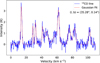 |
Fig. 1 Fit result of Gausspyplus at the position (1, b) = (35.28°, 0.14°). The blue curve represents the original 13CO (J = 1−0) spectrum, and the dashed red line indicates the Gaussian fitting curve. |
3.2 Filament morphology in G34
Based on the CO isotopes to trace the spatial and kinematic structure of the G34 molecular gas and considering the Gaussian fitting of the CO spectral lines with the determination coefficient (calculated as described in Appendix A.1), the coefficients of determination for 12CO, 13CO, and C18O are 0.988, 0.934, and 0.353, respectively. The results show that Gausspyplus has a weaker fitting for C18O because the signal is lower and the signal-to-noise ratio of C18O is lower, but it performs well for 13CO and 12CO.
Additionally, we present the integrated intensity, velocity, and velocity dispersion distributions of the Gausspyplus fitting for 12CO and C18O in Fig. B.1. The results show that 12CO traces a more diffuse region than 13CO (Fig. 2). The diffuse gas structure indicates that filaments F1 and F2 (see definitions in Sect. 3.2.1) have started to interact and form a bridge-like structure. According to Su et al. (2019), 12CO can trace diffuse gas structures and distributions with typical densities of 102 cm−3. The optically thinner C18O (Fig. B.1) and 13CO (Fig. 2) trace denser regions than 12CO, with typical values of 103−104 cm−3 (Su et al. 2019), but C18O does not effectively trace the entire filament skeleton. We therefore relied more on 13CO data to trace the relatively dense centers and filament structures in the molecular cloud.
For the kinematic distance of the G34 region, we used the parallax-based distance calculator V2 (Reid et al. 2016, 2019) provided by The Bar And Spiral Structure Legacy (BeSSeL) Survey project5. By adopting a position in G34 (l = 34.37°, b = −0.56°, VLSR = 13.0 km s−1), we obtained a kinematic distance of 2.12 ± 0.38 kpc. This corresponds to the far distance solution, with the highest probability of 69%. With this distance, G34 is located on the Carina-Sagittarius arm.
3.2.1 Moment maps
The 13CO integrated-intensity map for the local standard of rest (LSR) velocity range of 0–20 km s−1, as shown in Fig. 2a, clearly reveals two filaments. The identified two giant filaments are represented by the black curves in the three panels of Fig. 2. The identification of F1 and F2, along with the detailed parameter settings, is described in Sect. 3.3. We defined F1 as the eastern and F2 as the western filament structure. In the integrated-intensity map, clumps that are distributed along the two filaments are visible; the method and parameters we used to identify the clumps are provided in Sect. 3.6. The different distributions of the clumps may result from the material in the two filaments that converge toward the gravitational center. The distribution of the mass and clumps is discussed in detail in Sect. 4.1.
The velocity distribution of the 13CO molecular gas is shown in Fig. 2b. The results preliminarily indicate large-scale velocity gradients in the two filaments. Fig. 5 shows the 13CO velocity channel map. In F1, the velocity increases from the northeast and southeast toward the west and rises from 9.5 km s−1 at both ends to 15 km s−1 in the middle. In F2, the velocity increases from the northwest to the southeast and ranges from 7.5 km s−1 to 15 km s−1. The origin of the large-scale velocity gradients is discussed in detail in Sect. 4.2.
The velocity dispersion of 13CO is shown in Fig. 2c. The results indicate a higher velocity dispersion at the boundaries where the two filaments are close to each other. This dispersion might be caused by supersonic turbulence. The angular size of the H II region in the northwest corner, G32.80+0.19 (Gomez etal. 1995) is approximately 3.3″ × 3.3″ (markedby a white cross in Fig. 2c). The higher velocity dispersion in this area might be caused the expansion of the H II region, which enhances the local turbulence. This is evident from the high intensity and velocity in the moment-0 and moment-1 maps. The focus of this study is the large-scale structure of the filaments, and we do not discuss the thermal motion in this local region in detail.
3.2.2 H2 column density
Considering the complex velocity components in the G34 region, as shown in Figs. 1 and A.1, we did not use the dust emission to calculate the H2 column density  . We instead used the Xfactor, defined as
  , where ICO is the 13CO integrated intensity. Following Benedettini et al. (2020), we adopted a value of Xfactor = (1.2 ± 0.4) × 1021 cm−2 (K km s−1)−1 for 13CO (J = 1−0). The authors derived the H2 column densities from Herschel dust emission through an SED fit with four far-infrared bands (160–500 μm) and assumed a dust opacity law κλ = κ300 (λ / 300 μm)–β with κ300 = 0.1 cm2 g−1, a gas-to-dust ratio = 100, and a grain emissivity parameter β = 2. By calculating the integrated intensity of the single-velocity component 13CO emission, they obtained the average Xfactor as the ratio of
  and
and  . As noted by Benedettini et al. (2020), 13CO (J = 1−0) typically has low optical depths (τ < 1) in their dataset, however. In some dense regions, 13CO may become optically thick, which might lead to an underestimation of
  . In our analysis of the G34 region, we calculated the optical depth of 13CO and found that 95.12% of the pixels have
  (see Appendix A.2 for details). Therefore, in most areas, 13CO remains optically thin, and the use of Xfactor is valid. In the parts of G34 with the highest column density, however,
  derived from Xfactor should be considered a lower limit. It also is important to note that this Xfactor was derived in the third quadrant (i.e., 220° < 1 < 240°, −2.5° < b < 0°), which may introduce some errors for the G34 region, which is located in the first quadrant.
We summed in Sect. 3.1 the multicomponent integrated intensities, and here, ICO refers to the total integrated intensity between 0 and 20 km s−1 after summation. To obtain the average H2 column density for F1 and F2 separately, we used the masks for F1 and F2 created in Sect. 3.3, with the detailed parameter settings that are also provided in Sect. 3.3. The boundaries of the masks are shown in Fig. 2. We extracted the H2 column density for the F1 and F2 regions using these masks and calculated the averages. The average H2 column density values for the F1 and F2 regions are (6.00 ± 2.00) × 1021 cm−2 and (6.40 ± 2.13) × 1021 cm−2, respectively, as shown in Table 1. The uncertainty arises from the Xfactor error. The same masks were also used to extract the values for the total mass, average dust temperature Td, average nonthermal velocity dispersion σNT, sound speed cs, and average velocity for F1 and F2. The relevant calculations are presented in the following sections.
Observational studies by Onishi et al. (1998), Johnstone et al. (2004), Kirk et al. (2006), and André et al. (2010, 2014) indicated star formation is triggered at a certain threshold of the column density, approximately 8 × 1021 cm−2. Fig. 3 shows the histograms of the H2 column density for F1 and F2, as well as the distribution of the H2 volume density calculated from the widths of F1 and F2 that we fit in Sect. 3.4. For the column density distributions of F1 and F2, 16.77% and 22.70% of the pixels provide values greater than 8 × 1021 cm−2, respectively. This is roughly consistent with the description by Zucker & Chen (2018), who reported that the giant molecular filaments (GMFs) are predominantly composed of lower column density gas and that more than 75% of the gas lies below  cm−2. With
  cm−2 as the threshold for gas with a high column density (Zucker & Chen 2018), the fractions of the high column density gas in F1 and F2 are 4.16% and 8.33%, respectively. These statistics are lower than those described by Zucker & Chen (2018), compared with Milky Way Bone (45–50%), Minimus Spanning Tree (MST) Bone filaments (45–50%), and Large-scale Herschel filaments (30%). GMFs typically have a high column density fraction of about 10%. The H2 column density statistics suggest that F1 and F2 may be in an early evolutionary stage, with the possibility of current low-mass star formation.
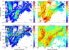 |
Fig. 2 Plots of the main skeleton of the two filaments identified by Filfinder in black lines on the map. The closed contours in the four panels indicate the boundaries of the F1 and F2 masks created in Sect. 3.3, which are shown in red in panels a and c and in black in panels b and d. (a) Integrated-intensity moment-0 map for 13CO (J = 1−0), integrated over the velocity range of 0–20 km s−1 toward G34. The white and red circles mark the dense clumps identified in Sect. 3.6, and red circles represet clumps in a state of virial collapse. The clump IDs correspond to those listed in Table 2. The beam size is shown in the bottom left corner, and the scale length of 10 pc is shown in the bottom right corner, (b) The 13CO LSR velocity moment-1 map shows the different velocity gradients within the two filaments, (c) 13CO full width to half-power moment-2 map showing the higher velocity dispersion in the gravitational centers of the two filaments. The white cross marks the H II region G32.80+0.19, which may cause the high-velocity dispersion, (d) Excitation temperature (Tex) distribution derived from 12CO (J = 1−0). See Sect. 3.3 for the calculation details. |
Physical parameters of the filaments
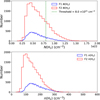 |
Fig. 3 Histograms of the H2 column density and H2 volume density from the masked areas defined in Sect. 3.3 for F1 and F2. The dashed green line in the upper panel represents the minimum H2 column density threshold for star formation. |
3.2.3 Infrared emission
We used the WISE three-color composite image at 3.4, 12, and 22 μm. The result is shown in Fig. 4. We used the WISE catalog of Galactic H II regions (Anderson et al. 2014, 2015a, 2018, 2019; Makai et al. 2017; Brown et al. 2017; Wenger et al. 2019) and selected the H II regions whose central coordinates fall within the Galactic longitude range [32°, 36°] and latitude range [−2°, 1°], which corresponds to the G34 region. To further select H II regions that are consistent with the G34 filament structure, we retained only those with distances within 2.12 ± 0.38 kpc, specifically, in the range of [1.74, 2.5] kpc, as well as those without distance information. We also excluded H II regions with radii smaller than 90″, which corresponds to three pixel sizes, because small regions like this are unlikely to significantly impact the large-scale dynamics of F1 and F2. The filtered results are indicated by cyan circles in Fig. 4. Among them, two green circles contain distance information within the range of [1.74, 2.5] kpc, specifically, at 2.33 ± 0.22 kpc (Wu et al. 2014) and 2.09 ± 0.25 kpc (Anderson et al. 2015b), with radii of 160″ and 170″, respectively. We considered them to possibly lie within the G34 filament structure. When we combined all filtered H II regions, however, the distribution of the H II regions did not correlate with the V-shaped curvature of the G34 filament structure.
We also marked the dense clumps identified by astrodendro in Fig. 4, for detailed settings (see Sect. 3.6), and the physical properties of the clumps are listed in Table 2. Star formation occurs in different parts of the filamentary gas, and the 22 μm emission conveniently traces star formation within molecular clouds. Only the location of clump 9 agrees with the red thermal dust core traced by WISE at 22 μm, and we found no other clumps. The reason might be that G34 is located in the tangential direction of the Carina–Sagittarius arm, with interference from foreground and background, similar to W51, which is also located in the Carina-Sagittarius arm (Reid et al. 2009, 2014) and lies at a distance of approximately 5.1 kpc from us (Sato et al. 2010). It might also be possible that this clump is in the process of star formation. This is consistent with the results in Sect. 3.2.2, which suggest that F1 and F2 may be in early evolutionary stages and may currently only form low-mass stars.
3.3 Physical parameter of the filaments
We used Filfinder (Koch & Rosolowsky 2015) to identify filaments in the G34 region based on H2 column density data. During the image preprocessing stage in Filfinder, we set flatten_percent=95, which calculates a normalized threshold by specifying the percentile of the image data. Specifically, we calculated the 95th percentile of the H2 column density data by sorting all pixel values of  from smallest to largest, and selecting the value at the 95% position. This threshold value helped us to ensure that brighter points (e.g., compact sources) did not interfere with the subsequent processing. Next, an arctan transformation was applied to enhance the image contrast and make bright and dark areas visually more distinct.
In the mask-creation stage, we set adapt_thresh = 100 pixels. 100 pixels correspond to 3000″, 50′or almost a full degree, meaning that filaments narrower than 100 pixels were not identified. We also set smooth_size = 100 pixels, the maximum scale for smoothing. By smoothing on a small scale, small noisy variations were removed, which resulted in a simpler skeleton structure. We used size_thresh = 400 pixel2, the minimum number of pixels for the mask region, to ensure that small discrete regions were not used to create the mask. The glob_thresh was set to 3.12 × 10²¹, defining the minimum H2 column density threshold. Data below this threshold were not used to create the mask; here, the intensity threshold was defined for signal regions greater than 5σ. The created mask is shown in Fig. C.1a. After creating the mask and identifying the filaments, we removed all branches and only retained the main trunks, as shown by the black curves in the three panels of Fig. 2.
Based on the kinematic distance determined in Sect. 3.2 and on the resolution of the CO data, we determined the actual size of each pixel in the G34 region. Using the filament skeleton pixel length we identified, we derived the actual filament length, as shown in Table 1. The lengths of F1 and F2 are 119.36 ± 21.39 pc and 150.79 ± 27.03 pc, respectively. The uncertainty arises from the distance measurement error. This is consistent with the length range of GMFs described by Zucker et al. (2019), which is between 100 and 200 pc. The calculation of the filament mass is based on the H2 column density, using the method proposed by Ma et al. (2023),
 (1)
(1)
Apixel is the area of a pixel, N(H2)pixel is the H2 column density derived from 13CO, μΗ = 2.8 (Kauffmann et al. 2008) is the mean molecular weight, and mH is the mass of a hydrogen atom. The pixels in the filament were extracted with the masks created by Filfmder during the filament identification process. By summing the H2 column density of each pixel within the mask and using Equation (1), we calculated the total masses of F1 and F2, which are (1.61 ± 1.22) × 10s Μ⊙ and (1.94 ± 1.47) x 10s Μ⊙, respectively. The uncertainty arises from the distance and Xfactor errors. Using the total mass and length calculated for F1 and F2, we derived the line mass Mline. The results are shown in Table 1, where the Mline for F1 and F2 are 1350 ± 511 M⊙ pe−1 and 1285 ± 486 M⊙ pe−1, respectively. The uncertainties in the total mass and line mass once again arise from the uncertainties in the distance and Xfactor parameters. The values are very high but still consistent with the highest line mass of approximately 1500 Μ⊙ pc−1 suggested by Zucker et al. (2019) for GMFs.
To estimate the kinetic temperature, we assumed that the molecular cloud G34 is under local thermodynamic equilibrium (LTE) conditions, such that Tgas = Tk = Tex. Assuming that 12CO is optically thick, we derived the excitation temperature (Tex) from the 12CO (J = 1−0) line emission following Garden et al. (1991), Nishimura et al. (2015), and Xu et al. (2018),
![Mathematical equation: ${T_{{\rm{ex}}}} = {{5.53} \over {\ln \left[ {1 + {{5.53} \over {T_{{\rm{mb}}}^*\left( {^{12}{\rm{CO}}} \right) + 0.819}}} \right]}},$](/articles/aa/full_html/2025/09/aa53851-25/aa53851-25-eq16.png) (2)
(2)
where  is the peak main-beam brightness temperature of 12CO, derived from the line profiles fit using Gausspyplus. for filaments F1 and F2, the average excitation temperatures are estimated to be 8 K, respectively. The results are shown in Table 1. Under the LTE assumption (Tk = Tex), we calculated the nonthermal velocity dispersion σNT (Liu et al. 2019; Tang et al. 2017) and the average sound speed cs for F1 and F2 as
 (3)
(3)
 (4)
(4)
where ΔVobs is the observed line width (FWHM) of 13CO (1−0), obtained from the Gaussian fitting results using Gausspyplus. kB is the Boltzmann constant, Tk is the kinetic temperature, μp = 2.33 is the mean molecular weight adopted from Kauffmann et al. (2008), and mobs is the molecular weight of the observed molecule, which is 29 for 13CO. The results are shown in Table 1. The uncertainties in σNT and cs arise from the fitting errors in determining the FWHM(13CO) and  . Studies involving ammonia (NH3) or formaldehyde (H2CO) allow the direct determination of Tk (Tang et al. 2017; Tursun et al. 2020).
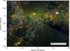 |
Fig. 4 Three-color composite image of WISE 3.4, 12, and 22 μm bands (background). Red, green, and blue represent 22, 12, and 3.4 μm, respectively. The white contours represent the integrated intensity of 13CO, with values ranging from 3 to 49 K km s−1 with a step size of 1.2 K km s−1 integrated between 0 and 20 km s−1. The cyan and green circles indicate H II regions cataloged by WISE in the Galaxy, where green circles indicate H II regions that are likely within the same area in G34. The red and yellow circles denote the dense clumps identified by Astrodendro, with red circles indicating virially collapsing clumps. The numbers within the circles correspond to the clump numbers in the second row of the panels in Fig. 8. The red curves highlight the skeletons of the two filaments identified by Filfinder. |
Physical parameters of the clumps.
3.4 Plummer-like profile fitting
For the width estimation of F1 and F2, we used Radfil (Zucker & Chen 2018), which is an interstellar filament profile density construction and fitting tool6. The fit was performed using a Plummer-like function (Cox et al. 2016),
![Mathematical equation: $N\left( r \right) = {{{N_0}} \over {{{\left[ {1 + {{\left( {{r \over {{R_{{\rm{flat}}}}}}} \right)}^2}} \right]}^{{{p - 1} \over 2}}}}},$](/articles/aa/full_html/2025/09/aa53851-25/aa53851-25-eq138.png) (5)
(5)
where N0 is the peak height of the profile, Rflat is the flattening radius, and p is the density profile index (Cox et al. 2016). It is important to note that the fitting procedure assumes an inclination of 0 for the filament with respect to the plane of the sky. The fitting process used the H2 column density, as well as the mask and filament spine identified by Filfinder, and a distance d = 2.12 ± 0.38 kpc (see Sect. 3.2) was adopted for the following analysis in physical units.
Using the builc_profile function in Radfil, we constructed the filament density profile. To achieve more accurate fitting results, we used the highest width sampling frequency samp_int=1, which can be roughly considered as drawing a line perpendicular to the filament at each pixel of the spine. More details can be found in Zucker & Chen (2018). The distribution of the density profile is shown in Fig.C.1a. The fit_profile function was used to fit the main profile of the filament with the Plummer model, selecting relatively flat regions of the profile density distribution to fit a first-order polynomial and subtracting the background. The fit results are shown in Figs.C.1b and c. The results of the filament width sampling are shown in Fig.C.1a. For better visualization, we reduced the width sampling frequency to samp_int=5. Following Hacar et al. (2023),  . The calculated filament width (FWHM) is shown in Table 1. The widths of F1 and F2 are 11.13 ± 2.0pc and 14.16 ± 2.5pc, respectively. The uncertainty arises from the distance measurement error. This is consistent with the width range of 10–20 pc for GMFs described by Zucker et al. (2019).
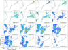 |
Fig. 5 13CO velocity channel map, with a velocity range of 7.5 km s−1 to 15.0 km s−1 and a step size of 0.5 km s−1. The 13CO integrated intensity is shown as the background. The magenta contours represent the 13CO integrated intensity, with levels ranging from 0.8 Κ km s−1 to 11.8 Κ km s−1 in steps of 0.8 Κ km s−1. The black curves indicate the skeleton structures of F1 and F2. |
3.5 Filament structure in G34
3.5.1 Distribution of the filament positions
It is important to emphasize that we can only obtain the velocity along the line of sight. To study the interaction between the two filaments, we propose a geometric model of the spatial distribution of F1 and F2, as shown in Figure 6. In this geometric model, we make some assumptions: (a) F1 and F2 approximately face the observer, meaning that the inclination angles of F1 and F2 are 0°. (b) The part of F1 in the center, where the filament seems to be closest to F2, is redshifted, suggesting that it is grav-itationally attracted to F2, which implies that F2 is slightly more distant.
Under these assumptions, the relative velocity vr (including the systemic velocity) of F1 and F2 has a certain angle θ with the line-of-sight velocity v. The relative velocity can be expressed as
 (6)
(6)
The parameter d indicates the unit distance perpendicular to the line of sight. To calculate the gravitational interaction between the two filaments, we need to know the real distance dr between F1 and F2, which can similarly be expressed using the angle θ,
 (7)
(7)
Another critical issue is that we need to know the range of the angle θ. In Section 3.2, we already calculated the kinematic distance of G34 and its uncertainty. From the calculation of the kinematic distance, F1 and F2 have similar velocities and are in the same region of the sky, so that it is highly probable that F1 and F2 are part of the same molecular complex in space. Therefore, we used derr = 380pc (see Sect. 3.2), the kinematic distance uncertainty, to represent the maximum distance difference between F1 and F2 along the line of sight, and we used d0 = 19.24 ± 3.45 pc to indicate the distance difference between F1 and F2 in the plane perpendicular to the line of sight. By using tan θ = d0/derr, we calculated the range of θ, which is (3.0°, 90°).
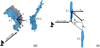 |
Fig. 6 (a) Spatial distribution of F1 and F2. The shadow behind F1 represents its projection onto the plane of the sky. (b) Top view of the spatial distribution of F1 and F2. The angle θ represents the angle between the line-of-sight velocity v and the approaching velocity vr, and d denotes the unit distance perpendicular to the line-of-sight plane. derr indicates the distance difference between F1 and F2 from Earth, and d0 is the distance difference perpendicular to the line of sight of the two ends of the two filaments. d0 is also marked in Fig. 7. |
3.5.2 Gravitational forces and potentials
To explore the gravitational interaction between F1 and F2, we extracted the two-dimensional surface density distributions,  μmΗ (i = 1, 2). Using the algorithm7 proposed by He et al. (2023b), we solved the 2D Poisson equation in Fourier space using the fast Fourier transform (FFT) to obtain the gravitational potential Φ. Specifically, we calculated the gravitational potentials (ΦF1, ΦF2) for F1 and F2, respectively, by first solving in the complex frequency domain and then applying an inverse FFT to transform the results back to the spatial domain. The gravitational potential Φ can be derived by solving Poisson’s equation,
 (8)
(8)
where G is the gravitational constant, and ρ(x, y) is the mass density distribution, which we replaced by the two-dimensional surface density distribution. By taking the gradient of the potential, a = ∇Φ, we obtained the acceleration distributions (aF1, aF2) for the two filaments.
We defined the mutual gravitational force and potential as F1,mutual and Φ1,mutual for the effect of F2 on F1, and F2,mutual and Φ2,mutual for the effect of F1 on F2. The self-gravitational force and potential were defined as F1,self and Φ1,self for F1, and F2,self and Φ2,self for F2,
 (9)
(9)
 (10)
(10)
 (11)
(11)
 (12)
(12)
The results are shown in Fig. 7, where the intensity distributions of self-gravity and mutual gravity are displayed. We employed the geometric model from Sect. 3.5.1, assumed θ=45°, and used Eq. (7) to calculate the relative distance between F1 and F2 for the gravitational calculations. The regions with a stronger mutual gravity in F1 and F2 are concentrated in the central parts of the filaments, and the gravitational attraction increases gradually from the ends toward the center. The comparison with self-gravity also suggests possible gravitational interactions between F1 and F2. The self-gravity is generally stronger in the shell regions of F1 and F2, which may indicate signs of gravitational contraction inside the individual filaments.
3.5.3 Longitudinal profiles of the main skeleton in the filaments
Under the geometric model proposed in Sect. 3.5.1, we assumed θ = 45° to determine the variation in the relative velocity between F1 and F2, as well as the changes in gravitational potential, as shown in Fig. 8. The PV diagram shows that the velocity of F1 increases from the ends toward the center, and the velocity of F2 increases from the northwest to the southeast. This is consistent with the velocity channel maps in Fig. 5. The self-gravitational and mutual gravitational potentials of F1 also decrease from both ends toward the center. In F2, the gravitational potential decreases from the northwestern to the southeastern corner, which is in contrast to the increasing trend of the velocity. This suggests that the gravitational potential energy may be partially converted into kinetic energy. We discuss the correlation between velocity and gravitational potential in Sect. 4 in detail.
Notably, in the PV diagram, the position of the peak velocity in F1, which increases from both ends to the center, aligns with the low point of the mutual gravitational potential, which can also be observed from the velocity distribution shown in Fig. 2b and the mutual gravitational potential distribution in Fig. 7. In F2, however, the peak velocity and the low point of the mutual gravitational potential do not coincide. In Fig. 2b, the southeastern corner of F2 is more redshifted than its central region, which does not match the mutual gravitational center in Fig. 7 or the low point of the mutual gravitational potential in Fig. 8. Three main reasons may account for this: (a) Star formation activity may be present within F2, which might affect the local gravitational field. Table 1 shows that F2 has a higher mass and higher average H2 column density than F1, which makes it more favorable for star formation, (b) The inclination angle of F2 may not be zero, and the northwestern corner may be farther from us, while the southeastern corner is closer. Under the assumption that F1 has a zero inclination angle, the southeastern corner of F2 is closest to F1, while the northwestern corner is farthest. In this case, the low point of the gravitational potential in F2 aligns with the increase in the peak velocity, (c) In the PV diagram, the velocity is approximately proportional to the distance along the skeleton of F2, that is, v ∝ r, which may suggest that F2 rotates at a fixed angular velocity. The actual length of F2 is about 150 pc, however, and because the filament is not a rigid body, the maintenance of rotation over this long distance might lead to the fragmentation of the filament. To simplify our geometric model, we maintained the assumptions made in Sect. 3.5.1, namely that F1 and F2 approximately face the observer, with their inclination angles set to 0°, and F1 is in the foreground while F2 is in the background.
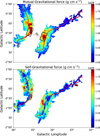 |
Fig. 7 Distribution of self-gravitational and mutual gravitational forces in F1 and F2. The red curves represent the spines of F1 and F2. The black boxes highlight the regions that are exposed to particularly high mutual gravity. The dashed line and d0 indicate the projected distance of the mutual centers of gravity. |
3.5.4 Stability of filaments
We calculated the line mass distribution of the filaments, defined as the mass per unit length Mline, using the radial density profiles created in Sect. 3.4 with Radfil, as done by Cox et al. (2016) and Li et al. (2022). The line mass was derived by integrating the radial density profile perpendicular to the main axis, defined as,
 (13)
(13)
where Apixel is the pixel area traversed by each red cut line shown in Fig. C.1a. The results of the line mass distribution are displayed in Fig. 9.
The significant curvature of the skeleton changes in the southeast corner of F1 and F2, however, and the width might be overestimated in some instances during the identification, as illustrated in Fig. C.1a. This overestimation leads to overlaps that correspond to the scattered points of Mline in the range of 0–20 pc in Fig. 9. Therefore, we focused on regions in which the curvature was relatively flat, which results in an accurate width identification and a continuous variation in the line mass that corresponds to the scattered points that are greater than 20 pc in Fig. 9. For F1 and F2, the intervals in which the line mass is greater than 2000 M⊙ pc−1 are [38.3, 81.8] pc and [20.2, 54.1] pc, respectively, which corresponds to the light green regions of Mline in Fig. 9 and to the red curves in the column density distribution map of the hydrogen molecule. In F1 and F2, the regions with a higher line mass are located in the central parts of the filament. This presents an inverse correlation with the distribution of the gravitational potential shown in Fig. 7, suggesting that gravity may influence the distribution of material inside the filaments to some extent.
At the same time, we also calculated the virial line mass for F1 and F2. Following Dewangan et al. (2019) and He et al. (2023a), Mline, vir was calculated as follows:
![Mathematical equation: ${M_{{\rm{line,vir}}}} = \left[ {1 + {{\left( {{{{\sigma _{{\rm{NT}}}}} \over {{c_{\rm{s}}}}}} \right)}^2}} \right] \times \left[ {16{{\rm{M}}_ \odot }{\rm{p}}{{\rm{c}}^{ - 1}} \times \left( {{{{T_{\rm{k}}}} \over {10\,{\rm{K}}}}} \right)} \right],$](/articles/aa/full_html/2025/09/aa53851-25/aa53851-25-eq149.png) (14)
(14)
where Tk is the kinetic temperature, cs is the sound speed, and σNT is the nonthermal line width. For local thermodynamic equilibrium (LTE), the kinetic temperature Tk is equal to the dust temperature Tdust. By extracting cs, σNT, and Tdust from the radial density profiles perpendicular to the main axis and calculating the average value along each vertical cut, we obtained the virial line mass at each sampling point. The results are shown as the red scatter points of Mline in the upper panels of Fig. 9. For F1 and F2, the virial line mass ranges are [35, 551] Μ⊙ pc−1 and [19, 324] Μ⊙ pc−1, which are lower than the line mass ranges of [548, 2700] M⊙ pc−1 and [442, 3700] M⊙ pc−1. According to Ostriker (1964) and Fischera & Martin (2012), the gravitational stability of a filament can be assessed using the ratio f ≡ Mline /Mline,vir. For F1 and F2, f is calculated to be 3.63 ± 1.38 and 4.19 ± 1.60, respectively, as listed in Table 1. Although these results suggest that F1 and F2 are gravitationally stable, the calculation of the virial line mass via Eq. (14) is based on several assumptions, namely, hydrostatic equilibrium, isolation, and isothermality. This may not hold for the observed filaments (Hacar et al. 2023). Moreover, the virial line mass was calculated without considering the contributions from magnetic pressure, which likely results in an underestimated virial mass.
To investigate this, we used the Planck 353 GHz data to map the magnetic field orientation (Planck Collaboration Int. XIX 2015). The magnetic field orientation angle ψB is given by the Stokes parameters Q and U as follows:
 (15)
(15)
The result is shown in Fig. 10, where we observe an ordered magnetic field nearly perpendicular to the G34 giant filaments. According to Li et al. (2015), this is a signature that the Lorentz force supports the filament against gravitational collapse along the direction perpendicular to the magnetic field lines. This indicates that, in addition to gravity, the magnetic field also plays a crucial role in the evolution of the G34 giant filaments. The filaments observed in the two-dimensional H2 column density map and the inferred magnetic field directions from the two-dimensional polarization map are results of line-of-sight integration, however. Therefore, the relative orientations measured in the two-dimensional sky map may not accurately represent the actual three-dimensional configuration.
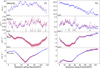 |
Fig. 8 Velocity variations along the spines of F1 and F2, along with the changes in the hydrogen column density, self-gravitational potential Φself, and mutual gravitational potential Φmutual. In the hydrogen column density panel, the positions and numbers of the corresponding clumps along the spines are labeled. The red labels indicate clumps that are in a state of virial collapse. The clump identification and detailed physical parameters are described in Sect. 3.6 and listed in Table 2. |
3.6 Stability of clumps
We used Astrodendro8 to identify the clumps. Astrodendro is a Python package for computing dendrograms of astronomical data. The data we used were the hydrogen molecule column density, as mentioned in Sect. 3.2.2, where the column density threshold for triggering star formation is approximately 8 × 1021 cm−2. Therefore, we set the minimum column density threshold for clump identification to 8.5 × 1021 cm−2, and we ultimately identified 16 clumps. The clump identification results are shown in Fig. 4. Following Seo et al. (2015), the virial mass was calculated as follows:
 (16)
(16)
Here, R is the semimajor axis of the ellipsoid representing a cloud, e is the eccentricity, G is the gravitational constant, and  is the representative value of total velocity dispersion within the clump, including the thermal and nonthermal motions. In this context, we used the average of the total velocity dispersion within the area of the clump. Assuming the dense clump is an ellipsoid with a density profile of ρ ~ r–β (Bertoldi & McKee 1992), we used β = 2 to estimate the virial mass. We further calculated the effective radius, mean dust temperature, average H2 column density, virial parameter, and surface density for each clump. The results are listed in Table 2. The identified clumps shown in Figs. 2a and 4 with red circles indicate clumps in a state of virial collapse. In the panels that show the hydrogen molecule column density in Fig. 8, the clumps at the corresponding positions in the skeleton are also marked with red short lines that indicate the positions of the clumps in virial collapse. Ignoring uncertainties from distance and the Xfactor, we find that only clump 13 has a virial parameter αvir > 2; the remaining clumps all have αvir < 2, which suggests that they are gravitationally bound and may be forming or are already forming stars. Additionally, clumps 5, 6, 9, 11, and 14 are located in the region between F1 and F2 and are already in a state of virial collapse. They might be affected by the asymmetric gravitational pull from the two filaments.
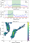 |
Fig. 9 Scatter points in the panels in the first and second row represent the variations of the line mass (blue) and the virial mass (red) for F1 and F2. The two green shaded areas represent the interval, where the line mass is greater than 2000 M⊙ pc−1. The background of the bottom panel shows the molecular hydrogen column density. The black curves correspond to the skeleton of F1 and F2, and the red curves correspond to the intervals of the skeleton marked by the green shaded areas in the upper panels. |
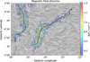 |
Fig. 10 H2 column density overlaid with magnetic field orientations based on Planck 353 GHz polarization measurements, visualized using the line-integral convolution (LIC) technique (Cabral & Leedom 1993). |
4 Discussion
4.1 Consistency of the gravitational potential and mass distribution
The velocity, gravitational potential in Fig. 8, and the line mass distribution in Fig. 9 show significant similarities. For F1, the velocity and line mass increase from the ends toward the center, while the gravitational potential decreases from the ends toward the center. In the column density map of the hydrogen molecule in Fig. 8, the clumps are concentrated in the right middle section, while clumps in a state of collapse are located near the gravitational potential minimum at the center. For F2, the distributions of the velocity and line mass increase from one end to the other, with the gravitational potential distribution being the opposite. In the variation of the hydrogen molecular column density, the clumps are concentrated at the end with a lower gravitational potential, while clumps in collapse are close to the center.
Therefore, we speculate that the mass distribution of F1 may be influenced by the gravitational pull exerted by F2, and similarly, the mass distribution of F2 may be influenced by the gravitational effect exerted by F1. This is evident from the inverse correlation between the mutual gravitational potential in Fig. 8 and the line mass variation in Fig. 11.
We plot the scatter diagram of the line mass and gravitational potential and performed a linear fitting, as shown in Fig. 11. For F1 and F2, the inverse correlation of the mutual gravitational potential with the line mass is stronger than that of the self-gravitational potential, as indicated by the Pearson correlation coefficients. This suggests that mutual gravitational attraction significantly influences the mass distribution. For F1, the absolute value of the Pearson correlation coefficient is greater than that for F2, indicating that the gravitational field of F2 has a stronger influence on F1. This is also reflected in Fig. 3 and Table 1, where the mass of F2 is greater than that of F1, leading to a greater gravitational influence on F1. This may also explain the formation of the V-shaped structure in F1. The results presented in Sect. 3.2.3 further suggest that the formation of the V-shaped structure and the possible mutual motion between F1 and F2 are not caused by the influence of H II regions generated by the intense star formation activity.
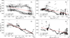 |
Fig. 11 Scatter plots of the line mass Mline vs. self-gravitational potential Φself (top two panels). Scatter plots of the line mass Μline vs. mutual gravitational potential Φmutual (bottom two panels). In all four panels, the red line represents the linear fitting result, and the Pearson correlation coefficient (r) and corresponding p-values is indicated in the bottom left corner of each panel. |
4.2 Do gravitational interactions lead to large-scale velocity gradients?
The trend of mutual gravitational attraction shown in Fig. 7 increases from the ends toward the center, which is consistent with the trend of velocity changes depicted in Fig. 8. Although we can only obtain the velocities along the line of sight and do not know the actual three-dimensional direction of the velocity, the statistical trend in Fig. 8 suggests that the velocities in F1 and F2 are broadly ordered on a large scale. This implies that the angles between the line-of-sight velocities and the actual velocity directions are likely consistent over a large area (even though there may be localized turbulent disturbances, similar to a river in which the overall flow direction is consistent, but local directions may vary). The trend in the line-of-sight velocities might therefore reflect the actual velocity variation to some extent.
The decreasing trend in the mutual gravitational potential approximately agrees with the increasing velocity trend. This indicates that the direction of the large-scale velocity may align with the direction of gravitational acceleration. It is also possible, though less likely, that the velocities are in the opposite direction to the acceleration, indicating deceleration. Consequently, we can roughly infer that gravitational interaction exists between F1 and F2, and they may continue to approach each other under the influence of mutual gravity.
In Sect. 4.1, the consistency between the velocity and gravitational potential distributions suggested that the velocity might be influenced by gravity, meaning that gravitational potential energy might be converted into kinetic energy. The observed velocity is along the line of sight, however, which means that by assuming that the angle is θ = 45° as shown in Fig. 6, we calculated the relative velocity Vr and relative distance dr between F1 and F2. We fit the relation between the velocity and gravitational potential using the equation V2 = ΑΦ + Β, where the constant A represents the proportional relation between the square of the velocity and the gravitational potential, and the constant Β is caused by the inherent initial velocity of the system. The results are shown in Fig. 12.
Considering different values of angle θ, we estimated the range of θ in Sect. 3.5.1. When θ is in the range of (3.0°, 90°), the Pearson correlation coefficients  , and
, and  consistently take values of −0.76± 0.05, – 0.95 ± 0.01, – 0.43 ± 0.09, and – 0.85 ± 0.03, indicating that the Pearson correlation coefficient does not strongly depend on the angle θ. Moreover, in all four panels of Fig. 12, the corresponding p-values are much lower than 0.01 (nearly zero), which is expected given the large sample size. These low p-values indicate that the calculated correlations are statistically significant. Based on the correlation coefficients, we find that the squared radial velocity versus the mutual gravitational potential for F1 and F2, and the squared radial velocity versus the self-gravitational potential for F2, are significantly and inversely correlated. This suggests that for both F1 and F2, the gravitational potential energy is to some extent converted into kinetic energy. For F2, the correlation between the gravitational potential and the square of the velocity is stronger than for F1. The mass of F2 is higher, however, and when the gravitational effects are considered alone, the correlation between the square of the velocity and the gravitational potential in F1 should be stronger due to the influence of the gravitational potential generated by F2. The actual situation is the opposite, however. This discrepancy might be caused by the greater impact of the turbulence on velocity the in F1 than in F2, as reflected in Table 1, where
  , meaning that the proportion of nonthermal components in F1 is greater than in F2.
Additionally, considering the distance factor between two pixels when calculating the gravitational potential, although the correlation between the square of velocity and self-gravitational potential is weaker, the order of magnitude of the potential is larger. Therefore, the proportion of potential energy converted into kinetic energy may not be smaller than that of the self-gravitational potential. Combined with the conclusions from Sect. 4.1, however, we can speculate that due to the influence of gravitational interactions, material in F1 flows toward the center, and in F2, material moves toward the region near one end. As material accumulates, the self-gravitational potential begins to play a role, further guides the flow of material, and might move the two filaments toward each other under mutual gravitational attraction. This is similar to the first stage described in the filaments-to-clusters paradigm by Kumar et al. (2020), where flow-driven filaments move closer together.
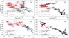 |
Fig. 12 Scatter plots of the radial velocity vs. the self-gravitational potential (top two panels), and scatter plots of the radial velocity vs. mutual gravitational potential (bottom two panels). The blue lines in all four panels represent the fitting lines of the square of velocity and gravitational potential, and the red scatter points indicate the regions in which Mline > 2000 M⊙ pc−1. The Pearson correlation coefficients (r) and corresponding p-values between velocity squared and gravitational potential are shown in the bottom left corner of each panel. |
4.3 Merging timescale
From the distribution of hydrogen molecular column density and linear mass, unlike the terminal collapse described by Burkert & Hartmann (2004); Yuan et al. (2020), the mass of F1 accumulates in the middle of the filament under the gravitational influence of F2, while the mass of F2 accumulates at one end of the filament under the gravitational influence of F1, without forming a terminal collapse effect. For the calculation, it is therefore unnecessary to consider the competition between the collapse timescale and the merging timescale (Hoemann et al. 2021, 2024). Following the merging timescale for two parallel cylinders proposed by Hoemann et al. (2021),
![Mathematical equation: $\matrix{ {{t_{{\rm{merge}}}} = \sqrt {{\pi \over {G\left( {{u_1} + {u_2}} \right)}}} {{{d_{\rm{r}}}} \over 2}\exp \left( {{{\upsilon _{\rm{r}}^2} \over {4G\left( {{u_1} + {u_2}} \right)}}} \right)} \hfill \cr {\,\,\,\,\,\,\,\,\,\, \times \left[ {1 - {\rm{erf}}\left( {{{{\upsilon _{\rm{r}}}} \over {\sqrt {4G\left( {{u_1} + {u_2}} \right)} }}} \right)} \right],} \hfill \cr } $](/articles/aa/full_html/2025/09/aa53851-25/aa53851-25-eq156.png) (17)
(17)
where G is the gravitational constant, u1 and u2 are the initial linear masses of the two filaments, dr is the initial distance, υr is the initial relative velocity, and erf(x) is the Gaussian error function.
Although the above formula calculates the merging timescale for two parallel cylinders, according to Hoemann et al. (2021), it also provides a good first-order approximation for inclined filaments.
The initial distance between the two filaments d0 = 19.24 ± 3.45 pc represents the projected distance between the centers of mutual gravity of F1 and F2, as shown in Fig.7. The initial average relative velocity υ0 = 1.05 km s−1, calculated similarly as the H2 column density, can be found in Sect. 3.2.2. The initial average line masses of F1 and F2 as u1 = 1350± 511 M⊙ pc−1 and u2 = 1285 ± 486 M⊙ pc−1, respectively. In Sect. 3.5.1 we estimated the range of θ as (3.0°, 90°). Based on Eqs. (6), (7), and (17), we can derive the functional relation between tmerge and θ, as shown in Fig. 13, with the error stemming from the distance uncertainty. The minimum merger time is 0.48 ± 0.15 Myr, and the maximum time is 56.73 ± 18.67 Myr. Sorting the merging times in ascending order and selecting the value corresponding to the 60% position yields a merging time of 34.23 ± 11.31 Myr. When θ = 45°, dr = 27.21 ± 4.88 pc and υr = 1.39 km s−1, which leads to a corresponding merger time of 4.62 ± 1.12 Myr, as shown in Fig. 13.
Combining the conclusions of Sect. 4.2, we propose three stages for the merging of the two filaments in G34: First, the filaments transport material toward the gravitational center under mutual gravitational influence. Second, as the material accumulates at the gravitational center, self-gravity begins to guide the material flow toward the center. Finally, when the central material accumulation reaches the supply limit of the filament, the two filaments move toward each other under mutual gravitational influence and may collide after approximately 4.62 ± 1.12 Myr.
Within the estimated merging timescale of the two filaments, stellar feedback from dense gas regions inside F1 and F2 might affect the outcome of the collision. Our observations only provide a snapshot of the evolutionary stage of the filament, and although we cannot precisely estimate the timescale along which the internal dense regions of F1 and F2 undergo gravitational collapse, form protostars, and ultimately develop into stellar feedback that disrupts the parental molecular cloud, previous studies offered useful constraints. For example, Chevance et al. (2020) statistically estimated the lifetimes and feedback timescales of giant molecular clouds (GMC) that actively form stars in nearby disc galaxies. By analyzing the CO-to-Ηα flux ratio, they inferred typical GMC lifetimes of about 10–30 Myr. When massive stars form, early stellar feedback may disperse the parental GMC within 1–5 Myr. These timescales fall within the range of our estimated filament merging timescale, suggesting that the outcome of the F1–F2 collision might be influenced by feedback processes originating from star formation that occurs within the filaments themselves. Although the time estimates of both are rather rough, this also reveals the possibility that the collision outcome might be affected by the feedback from the stars that formed inside the F1 and F2 merging timescales.
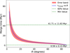 |
Fig. 13 Function of tmerge as a function of θ (blue curve), where θ is the angle between vr and v, as shown in Fig. 6. The red area indicates the error band, and the horizontal green lines represent the minimum merger time corresponding to 60% value, which is obtained by sorting the merger times in ascending order and selecting the value at the 60% position between the minimum and maximum. |
5 Conclusion
The G34 giant molecular cloud is considered a candidate for colliding filaments and serves as an example of flow-driven converging filaments in the first stage of the filaments-to-clusters paradigm described by Kumar et al. (2020). We reported the observation results of the Milky Way Imaging Scroll Painting (MWISP) for the giant filament G34 in the 13CO and 12CO spectral line. The distributions of the integrated intensity, velocity, H2 column density, line width, 12CO excitation temperature, self-gravity, and mutual gravity were presented. By fitting the F1 and F2 filaments with a Plummer-like profile, we obtained their lengths and widths.
In the giant molecular cloud G34, taking
 cm−2 as the threshold for high column density gas, the fractions of high column density gas in F1 and F2 are 4.16% and 8.33%, respectively. They are lower than the results described by Zucker & Chen (2018), where the typical fraction of high column density gas in giant molecular filaments (GMFs) was about 10%. This suggests that F1 and F2 may reside in early evolutionary stages and might be forming low-mass stars.
We calculated the line mass Mline of the filaments along the skeletons of F1 and F2 and found that Mline,vir is significantly lower than Mline, indicating that factors supporting the filaments, in addition to gravity and thermal pressure, also include significant contributions from magnetic fields and turbulence. We also observed that the ordered magnetic fields are nearly perpendicular to F1 and F2, which is a signature of Lorentz forces supporting the filaments against gravitational collapse in directions perpendicular to the magnetic field lines. (Li et al. 2015). This suggests that during the evolution of F1 and F2, magnetic fields play a crucial role together with gravity.
F1 and F2 both exhibit large-scale velocity gradients that span the entire filaments. Moreover, the trend in velocity change is similar to that of the line mass variation and is inversely correlated with the change in gravitational potential. This may indicate a transformation between kinetic and gravitational potential energy between F1 and F2. Furthermore, we investigated the NASA Wide-field Infrared Survey Explorer (WISE) data of galactic H II regions and found no H II regions that correlated with the shapes of F1 and F2. This indicates that the material distribution within F1 and F2, as well as the V-shaped structure of F1, is not influenced by feedback from H II regions, but is instead caused by gravitational effects.
In F1, material primarily accumulates in the middle of the filament, while in F2, it mainly accumulates at one end of the filament. This does not produce the end-cap collapse effect described by Burkert & Hartmann (2004), Yuan et al. (2020), and Hoemann et al. (2024), and therefore, the collapse and merging timescales do not compete. We proposed three stages of filament merging in G34. First, mutual gravitational attraction gradually causes the material in F1 and F2 to cluster toward the mutual center of gravity. Second, the self-gravity generated by the accumulating material guides the filament material to flow further inward. Finally, the materials clustered in the center from the previous two stages moves toward each other under mutual gravitational influence and may merge in approximately 4.62 ± 1.12 Myr. This merging process might be affected by additional stellar feedback arising from star formation within the dense regions of F1 and F2, however.
Acknowledgements
This work was main funded by National Key R&D Program of China under grant Nos. (2022YFA1603103 and 2023YFA1608002) and Tianshan Talent Training Program 2024TSYCTD0013. It was also partially funded by the Regional Collaborative Innovation Project of Xinjiang Uyghur Autonomous Region grant 2022E0105, the NSFC under grants 12173075, 11973076, 12103082 and 12403033, the CAS Light of West China Program 2021-XBQNXZ-028 and XBZG-ZDSYS-202212, the Xinjiang Key Laboratory of Radio Astrophysics under grant 2022D04033, The Tianshan Talent Program of Xinjiang Uygur Autonomous Region under Grant No. 2022TSYCLJ0005, the Youth Innovation Promotion Association CAS, the Tianchi Talent Project of Xinjiang Uyghur Autonomous Region. This research made use of the data from the Milky Way Imaging Scroll Painting (MWISP) project, which is a multiline survey in 12CO/13CO/C18O along the northern galactic plane with PMO-13.7m telescope. We are grateful to all the members of the MWISP working group, particularly the staff members at PMO-13.7m telescope, for their long-term support. MWISP was sponsored by the National Key R&D Program of China with grants 2023YFA1608000 and 2017YFA0402701 and by CAS Key Research Program of Frontier Sciences with grant QYZDJ-SSW-SLH047. C. Henkel has been funded by Chinese Academy of Sciences President’s International Fellowship Initiative grant No. 2025PVA0048. Sobolev Andrey has been funded by Chinese Academy of Sciences President’s International Fellowship Initiative grant No. 2024VMA0002.
Appendix A Gausspyplus fit result
A.1 Gausspyplus decomposition result
From the Gaussian fit results, the systemic velocity, line width, and intensity were extracted for each pixel. These three parameters determine a Gaussian function. Considering that each pixel may contain different velocity components, the Gaussian functions of these different velocity components were superimposed to obtain the Gaussian-fitted spectrum for each pixel. One of the fitting results are shown in Fig. 1.
At the same time, we also calculated the average spectrum of the entire image. The Gaussian-fitted spectra of each pixel were superimposed and averaged, and then compared with the average spectrum of the original data, as shown in Fig. A.1. By comparing the average spectrum and the Gaussian-fitted average spectrum, we calculated the coefficient of determination R2. The R2 value is defined as  , where yi is the observed value,
  is the fitted value, and
  is the mean of the observed values. It reflects the proportion of variance explained by the model–the higher the R2, the better the fit. For 12CO, 13CO and C18O, the coefficients of determination are 0.988, 0.934, and 0.353, respectively.
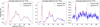 |
Fig. A.1 The figure shows the average spectra of the original data and the Gaussian fits for 12CO, 13CO and C18O, respectively. The red lines represent the Gaussian fit average spectra and the blue color represents the average spectra of the original data. |
A.2 Gaussian component distribution
The optical depth of 13CO is derived following Garden et al. (1991) and Pineda et al. (2010):
![Mathematical equation: ${\tau _{{{13}_{{\rm{CO}}}}}} = - \ln \left[ {1 - {{T_{{\rm{mb}}}^*\left( {^{13}{\rm{CO}}} \right)} \over {5.29}}{{\left( {{{\left( {\exp \left( {{{5.29} \over {{T_{{\rm{ex}}}}}}} \right) - 1} \right)}^{ - 1}} - 0.164} \right)}^{ - 1}}} \right].$](/articles/aa/full_html/2025/09/aa53851-25/aa53851-25-eq161.png) (A.1)
(A.1)
Here,  is the main beam brightness temperature of 13CO, and Tex is the excitation temperature of 12CO (J = 1−0). The calculation details are provided in Sect. 3.3. The pixel-by-pixel calculation results are shown in the panel (d) of Fig. A.2.
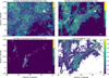 |
Fig. A.2 The red curves in the four panels represent the filament skeleton. (a) The background shows the number of Gaussian components of the 12CO spectra, with contours indicating the integrated intensity of 12CO in the range of 18 to 160 K km s−1, with a step size of 5 K km s−1. The integration velocity range is 0–20 km s−1, which is consistent across panels (b), (c), and (d). The beam size is shown in the bottom left corner, and the scale length of 10 pc is shown in the bottom right corner. (b) The background shows the number of Gaussian components of the 13CO spectra, with contours showing the integrated intensity of 13CO ranging from 3 to 49 K km s−1, with a step size of 1.2 K km s−1. (c) The background shows the number of Gaussian components of the C18O spectra, with contours showing the integrated intensity of C18O ranging from 0.5 to 7 K km s−1, with s step size of 1 K km s−1. (d) The background shows the optical depth of 13CO, with the same contours as in panel (b). |
Appendix B 12CO and C18O filament morphology in G34
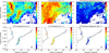 |
Fig. B.1 The black curves in all six panels indicate the filament skeletons. Panels (a) and (d) show the integrated-intensity maps of 12CO and C18O, respectively, with a velocity range of 0–20 km s−1. Panels (b) and (e) present the Local Standard of Rest (LSR) velocity maps of 12CO and C18O, respectively. Panels (c) and (f) display the velocity dispersion maps of 12CO and C18O, respectively. |
Appendix C Plummer like profile fit result
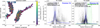 |
Fig. C.1 (a) Sampling results of filament width. The background is the H2 column density with the Filfinder mask applied. The red curves represents the filament spines. The thin red lines are vertical cuts perpendicular to the filament spine at each sampling interval. The blue dots are the density peaks on each cut. (b) and (c) The width fitting results for F1 and F2, along with the profile peak height, flattening radius, and density profile index, are noted in the upper left corner of the panels. The blue curves represent the Plummer function fitting curves, and the blue dashed line indicates the fitting interval of the Plummer function. The horizontal green solid line in the panel of (c) represents the fitting background straight line, and the green shaded region indicates the area of the baseline fitting, which uses a linear function, with the equation shown in the upper left corner of the panel. Due to the lack of a flatter region in the profile peak distribution of F1, the baseline fitting of the profile peak distribution is not performed for F1. |
References
- Anderson, L. D., Bania, T. M., Baiser, D. S., et al. 2014, ApJS, 212, 1 [NASA ADS] [CrossRef] [Google Scholar]
- Anderson, L. D., Armentrout, W. P., Johnstone, B. M., et al. 2015a, ApJS, 221, 26 [NASA ADS] [CrossRef] [Google Scholar]
- Anderson, L. D., Hough, L. A., Wenger, T. V., Bania, T. M., & Balser, D. S. 2015b, ApJ, 810, 42 [NASA ADS] [CrossRef] [Google Scholar]
- Anderson, L. D., Armentrout, W. P., Luisi, M., et al. 2018, ApJS, 234, 33 [NASA ADS] [CrossRef] [Google Scholar]
- Anderson, L. D., Wenger, T. V., Armentrout, W. P., Balser, D. S., & Bania, T. M. 2019, ApJ, 871, 145 [NASA ADS] [CrossRef] [Google Scholar]
- André, P., Men’shchikov, A., Bontemps, S., et al. 2010, A&A, 518, L102 [NASA ADS] [CrossRef] [EDP Sciences] [Google Scholar]
- André, P., Könyves, V., Arzoumanian, D., Palmeirim, P., & Peretto, N. 2013, in Astronomical Society of the Pacific Conference Series, 476, New Trends in Radio Astronomy in the ALMA Era: The 30th Anniversary of Nobeyama Radio Observatory, eds. R. Kawabe, N. Kuno, & S. Yamamoto, 95 [Google Scholar]
- André, P., Di Francesco, J., Ward-Thompson, D., et al. 2014, in Protostars and Planets VI, eds. H. Beuther, R. S. Klessen, C. P. Dullemond, & T. Henning, 27 [Google Scholar]
- Benedettini, M., Molinari, S., Baldeschi, A., et al. 2020, A&A, 633, A147 [NASA ADS] [CrossRef] [EDP Sciences] [Google Scholar]
- Bertoldi, F., & McKee, C. F. 1992, ApJ, 395, 140 [NASA ADS] [CrossRef] [Google Scholar]
- Birks, J. R., Fuller, G. A., & Gibb, A. G. 2006, A&A, 458, 181 [NASA ADS] [CrossRef] [EDP Sciences] [Google Scholar]
- Brown, C., Jordan, C., Dickey, J. M., et al. 2017, AJ, 154, 23 [Google Scholar]
- Burkert, A., & Hartmann, L. 2004, ApJ, 616, 288 [Google Scholar]
- Cabral, B., & Leedom, L. C. 1993, in Proceedings of the 20th Annual Conference on Computer Graphics and Interactive Techniques, SIGGRAPH ’93 (New York, NY, USA: Association for Computing Machinery), 263 [Google Scholar]
- Chevance, M., Kruijssen, J. M. D., Hygate, A. P. S., et al. 2020, MNRAS, 493, 2872 [NASA ADS] [CrossRef] [Google Scholar]
- Cosentino, G., Jiménez-Serra, I., Barnes, A. T., et al. 2025, A&A, 693, A199 [NASA ADS] [CrossRef] [EDP Sciences] [Google Scholar]
- Cox, N. L. J., Arzoumanian, D., André, P., et al. 2016, A&A, 590, A110 [NASA ADS] [CrossRef] [EDP Sciences] [Google Scholar]
- de Geus, E. J. 1992, A&A, 262, 258 [NASA ADS] [Google Scholar]
- Dewangan, L. K. 2017, ApJ, 837, 44 [Google Scholar]
- Dewangan, L. K., Pirogov, L. E., Ryabukhina, O. L., Ojha, D. K., & Zinchenko, I. 2019, ApJ, 877, 1 [Google Scholar]
- Elmegreen, B. G. 1998, in Astronomical Society of the Pacific Conference Series, 148, Origins, eds. C. E. Woodward, J. M. Shull, & H. A. Thronson, Jr., 150 [NASA ADS] [Google Scholar]
- Fischera, J., & Martin, P. G. 2012, A&A, 542, A77 [NASA ADS] [CrossRef] [EDP Sciences] [Google Scholar]
- Garden, R. P., Hayashi, M., Gatley, I., Hasegawa, T., & Kaifu, N. 1991, ApJ, 374, 540 [NASA ADS] [CrossRef] [Google Scholar]
- Gomez, Y., Garay, G., & Lizano, S. 1995, ApJ, 453, 727 [Google Scholar]
- Hacar, A., Tafalla, M., Kauffmann, J., & Kovács, A. 2013, A&A, 554, A55 [NASA ADS] [CrossRef] [EDP Sciences] [Google Scholar]
- Hacar, A., Clark, S. E., Heitsch, F., et al. 2023, in Astronomical Society of the Pacific Conference Series, 534, Protostars and Planets VII, eds. S. Inutsuka, Y. Aikawa, T. Muto, K. Tomida, & M. Tamura, 153 [NASA ADS] [Google Scholar]
- He, Y.-X., Liu, H.-L., Tang, X.-D., et al. 2023a, ApJ, 957, 61 [NASA ADS] [CrossRef] [Google Scholar]
- He, Z.-Z., Li, G.-X., & Burkert, A. 2023b, MNRAS, 526, L20 [NASA ADS] [CrossRef] [Google Scholar]
- Hennemann, M., Motte, F., Schneider, N., et al. 2012, A&A, 543, L3 [NASA ADS] [CrossRef] [EDP Sciences] [Google Scholar]
- Hoemann, E., Heigl, S., & Burkert, A. 2021, MNRAS, 507, 3486 [NASA ADS] [CrossRef] [Google Scholar]
- Hoemann, E., Socci, A., Heigl, S., Burkert, A., & Hacar, A. 2024, MNRAS, 532, L42 [NASA ADS] [CrossRef] [Google Scholar]
- Jackson, J. M., Finn, S. C., Chambers, E. T., Rathborne, J. M., & Simon, R. 2010, ApJ, 719, L185 [Google Scholar]
- Johnstone, D., Di Francesco, J., & Kirk, H. 2004, ApJ, 611, L45 [Google Scholar]
- Kashiwagi, R., Iwasaki, K., & Tomisaka, K. 2023, ApJ, 954, 129 [NASA ADS] [CrossRef] [Google Scholar]
- Kauffmann, J., Bertoldi, F., Bourke, T. L., Evans, N. J., I., & Lee, C. W. 2008, A&A, 487, 993 [NASA ADS] [CrossRef] [EDP Sciences] [Google Scholar]
- Kirk, H., Johnstone, D., & Di Francesco, J. 2006, ApJ, 646, 1009 [Google Scholar]
- Kirk, H., Myers, P. C., Bourke, T. L., et al. 2013, ApJ, 766, 115 [Google Scholar]
- Koch, E. W., & Rosolowsky, E. W. 2015, MNRAS, 452, 3435 [Google Scholar]
- Kumar, M. S. N., Palmeirim, P., Arzoumanian, D., & Inutsuka, S. I. 2020, A&A, 642, A87 [EDP Sciences] [Google Scholar]
- Li, G.-X., Wyrowski, F., Menten, K., & Belloche, A. 2013, A&A, 559, A34 [NASA ADS] [CrossRef] [EDP Sciences] [Google Scholar]
- Li, H.-B., Yuen, K. H., Otto, F., et al. 2015, Nature, 520, 518 [Google Scholar]
- Li, G.-X., Urquhart, J. S., Leurini, S., et al. 2016, A&A, 591, A5 [NASA ADS] [CrossRef] [EDP Sciences] [Google Scholar]
- Li, S., Sanhueza, P., Lee, C. W., et al. 2022, ApJ, 926, 165 [NASA ADS] [CrossRef] [Google Scholar]
- Lindner, R. R., Vera-Ciro, C., Murray, C. E., et al. 2015, AJ, 149, 138 [NASA ADS] [CrossRef] [Google Scholar]
- Liu, T., Zhang, Q., Kim, K.-T., et al. 2016, ApJ, 824, 31 [Google Scholar]
- Liu, H.-L., Stutz, A., & Yuan, J.-H. 2019, MNRAS, 487, 1259 [Google Scholar]
- Ma, Y., Zhou, J., Esimbek, J., et al. 2023, A&A, 676, A15 [NASA ADS] [CrossRef] [EDP Sciences] [Google Scholar]
- Makai, Z., Anderson, L. D., Mascoop, J. L., & Johnstone, B. 2017, ApJ, 846, 64 [Google Scholar]
- Mallick, K. K., Kumar, M. S. N., Ojha, D. K., et al. 2013, ApJ, 779, 113 [NASA ADS] [CrossRef] [Google Scholar]
- Mattern, M., Kauffmann, J., Csengeri, T., et al. 2018, A&A, 619, A166 [NASA ADS] [CrossRef] [EDP Sciences] [Google Scholar]
- Molinari, S., Swinyard, B., Bally, J., et al. 2010, A&A, 518, L100 [NASA ADS] [CrossRef] [EDP Sciences] [Google Scholar]
- Montillaud, J., Juvela, M., Vastel, C., et al. 2019, A&A, 631, A3 [NASA ADS] [CrossRef] [EDP Sciences] [Google Scholar]
- Myers, P. C. 2009, ApJ, 700, 1609 [Google Scholar]
- Nakamura, F., Sugitani, K., Tanaka, T., et al. 2014, ApJ, 791, L23 [NASA ADS] [CrossRef] [Google Scholar]
- Nishimura, A., Tokuda, K., Kimura, K., et al. 2015, ApJS, 216, 18 [NASA ADS] [CrossRef] [Google Scholar]
- Onishi, T., Mizuno, A., Kawamura, A., Ogawa, H., & Fukui, Y. 1998, ApJ, 502, 296 [NASA ADS] [CrossRef] [Google Scholar]
- Ostriker, J. 1964, ApJ, 140, 1056 [Google Scholar]
- Paron, S., & Weidmann, W. 2010, MNRAS, 408, 2487 [Google Scholar]
- Peretto, N., Fuller, G. A., Duarte-Cabral, A., et al. 2013, A&A, 555, A112 [NASA ADS] [CrossRef] [EDP Sciences] [Google Scholar]
- Pineda, J. L., Goldsmith, P. F., Chapman, N., et al. 2010, ApJ, 721, 686 [NASA ADS] [CrossRef] [Google Scholar]
- Planck Collaboration Int. XIX. 2015, A&A, 576, A104 [NASA ADS] [CrossRef] [EDP Sciences] [Google Scholar]
- Reid, M. J., Menten, K. M., Zheng, X. W., Brunthaler, A., & Xu, Y. 2009, ApJ, 705, 1548 [NASA ADS] [CrossRef] [Google Scholar]
- Reid, M. J., Menten, K. M., Brunthaler, A., et al. 2014, ApJ, 783, 130 [Google Scholar]
- Reid, M. J., Dame, T. M., Menten, K. M., & Brunthaler, A. 2016, ApJ, 823, 77 [Google Scholar]
- Reid, M. J., Menten, K. M., Brunthaler, A., et al. 2019, ApJ, 885, 131 [Google Scholar]
- Riener, M., Kainulainen, J., Henshaw, J. D., et al. 2019, A&A, 628, A78 [NASA ADS] [CrossRef] [EDP Sciences] [Google Scholar]
- Sánchez-Monge, Á., Beltrán, M. T., Cesaroni, R., et al. 2014, A&A, 569, A11 [NASA ADS] [CrossRef] [EDP Sciences] [Google Scholar]
- Sato, M., Reid, M. J., Brunthaler, A., & Menten, K. M. 2010, ApJ, 720, 1055 [Google Scholar]
- Schisano, E., Molinari, S., Elia, D., et al. 2020, MNRAS, 492, 5420 [Google Scholar]
- Schneider, N., Bontemps, S., Simon, R., et al. 2006, A&A, 458, 855 [NASA ADS] [CrossRef] [EDP Sciences] [Google Scholar]
- Schneider, N., Csengeri, T., Hennemann, M., et al. 2012, A&A, 540, L11 [NASA ADS] [CrossRef] [EDP Sciences] [Google Scholar]
- Schuller, F., Menten, K. M., Contreras, Y., et al. 2009, A&A, 504, 415 [NASA ADS] [CrossRef] [EDP Sciences] [Google Scholar]
- Seo, Y. M., Shirley, Y. L., Goldsmith, P., et al. 2015, ApJ, 805, 185 [Google Scholar]
- Su, Y., Yang, J., Zhang, S., et al. 2019, ApJS, 240, 9 [Google Scholar]
- Tachihara, K., Toyoda, S., Onishi, T., et al. 2001, PASJ, 53, 1081 [NASA ADS] [Google Scholar]
- Tan, W. S., Araya, E. D., Rigg, C., et al. 2023, ApJ, 953, 90 [Google Scholar]
- Tang, X. D., Henkel, C., Menten, K. M., et al. 2017, A&A, 598, A30 [NASA ADS] [CrossRef] [EDP Sciences] [Google Scholar]
- Tursun, K., Esimbek, J., Henkel, C., et al. 2020, A&A, 643, A178 [NASA ADS] [CrossRef] [EDP Sciences] [Google Scholar]
- Wang, K., Ge, Y., & Baug, T. 2024, A&A, 686, L11 [NASA ADS] [CrossRef] [EDP Sciences] [Google Scholar]
- Wenger, T. V., Dickey, J. M., Jordan, C. H., et al. 2019, ApJS, 240, 24 [Google Scholar]
- Whitworth, A. P. 2007, in IAU Symposium, 237, Triggered Star Formation in a Turbulent ISM, eds. B. G. Elmegreen, & J. Palous, 251 [Google Scholar]
- Wright, E. L., Eisenhardt, P. R. M., Mainzer, A. K., et al. 2010, AJ, 140, 1868 [Google Scholar]
- Wu, Y. W., Sato, M., Reid, M. J., et al. 2014, A&A, 566, A17 [NASA ADS] [CrossRef] [EDP Sciences] [Google Scholar]
- Xu, J.-L., Xu, Y., Zhang, C.-P., et al. 2018, A&A, 609, A43 [NASA ADS] [CrossRef] [EDP Sciences] [Google Scholar]
- Yuan, J., Li, J.-Z., Wu, Y., et al. 2018, ApJ, 852, 12 [Google Scholar]
- Yuan, L., Li, G.-X., Zhu, M., et al. 2020, A&A, 637, A67 [EDP Sciences] [Google Scholar]
- Zucker, C., & Chen, H. H.-H. 2018, ApJ, 864, 152 [NASA ADS] [CrossRef] [Google Scholar]
- Zucker, C., Smith, R., & Goodman, A. 2019, ApJ, 887, 186 [NASA ADS] [CrossRef] [Google Scholar]
Herschel: the ESA far-infrared space telescope.
SEDIGISM: Structure, Excitation, and Dynamics of the Inner Galactic InterStellar Medium.
Code source: Gausspyplus, available at https://github.com/mriener/gausspyplus
BeSSeL: Parallax-Based Distance Calculator V2 , available at http://bessel.vlbi-astrometry.org/node/378
Code source: Radfil, available at https://github.com/catherinezucker/radfil
Code source: Astronomical Dendrograms, available at http://www.dendrograms.org/
All Tables
All Figures
|
Fig. 1 Fit result of Gausspyplus at the position (1, b) = (35.28°, 0.14°). The blue curve represents the original 13CO (J = 1−0) spectrum, and the dashed red line indicates the Gaussian fitting curve. |
| In the text | |
|
Fig. 2 Plots of the main skeleton of the two filaments identified by Filfinder in black lines on the map. The closed contours in the four panels indicate the boundaries of the F1 and F2 masks created in Sect. 3.3, which are shown in red in panels a and c and in black in panels b and d. (a) Integrated-intensity moment-0 map for 13CO (J = 1−0), integrated over the velocity range of 0–20 km s−1 toward G34. The white and red circles mark the dense clumps identified in Sect. 3.6, and red circles represet clumps in a state of virial collapse. The clump IDs correspond to those listed in Table 2. The beam size is shown in the bottom left corner, and the scale length of 10 pc is shown in the bottom right corner, (b) The 13CO LSR velocity moment-1 map shows the different velocity gradients within the two filaments, (c) 13CO full width to half-power moment-2 map showing the higher velocity dispersion in the gravitational centers of the two filaments. The white cross marks the H II region G32.80+0.19, which may cause the high-velocity dispersion, (d) Excitation temperature (Tex) distribution derived from 12CO (J = 1−0). See Sect. 3.3 for the calculation details. |
| In the text | |
|
Fig. 3 Histograms of the H2 column density and H2 volume density from the masked areas defined in Sect. 3.3 for F1 and F2. The dashed green line in the upper panel represents the minimum H2 column density threshold for star formation. |
| In the text | |
|
Fig. 4 Three-color composite image of WISE 3.4, 12, and 22 μm bands (background). Red, green, and blue represent 22, 12, and 3.4 μm, respectively. The white contours represent the integrated intensity of 13CO, with values ranging from 3 to 49 K km s−1 with a step size of 1.2 K km s−1 integrated between 0 and 20 km s−1. The cyan and green circles indicate H II regions cataloged by WISE in the Galaxy, where green circles indicate H II regions that are likely within the same area in G34. The red and yellow circles denote the dense clumps identified by Astrodendro, with red circles indicating virially collapsing clumps. The numbers within the circles correspond to the clump numbers in the second row of the panels in Fig. 8. The red curves highlight the skeletons of the two filaments identified by Filfinder. |
| In the text | |
|
Fig. 5 13CO velocity channel map, with a velocity range of 7.5 km s−1 to 15.0 km s−1 and a step size of 0.5 km s−1. The 13CO integrated intensity is shown as the background. The magenta contours represent the 13CO integrated intensity, with levels ranging from 0.8 Κ km s−1 to 11.8 Κ km s−1 in steps of 0.8 Κ km s−1. The black curves indicate the skeleton structures of F1 and F2. |
| In the text | |
|
Fig. 6 (a) Spatial distribution of F1 and F2. The shadow behind F1 represents its projection onto the plane of the sky. (b) Top view of the spatial distribution of F1 and F2. The angle θ represents the angle between the line-of-sight velocity v and the approaching velocity vr, and d denotes the unit distance perpendicular to the line-of-sight plane. derr indicates the distance difference between F1 and F2 from Earth, and d0 is the distance difference perpendicular to the line of sight of the two ends of the two filaments. d0 is also marked in Fig. 7. |
| In the text | |
|
Fig. 7 Distribution of self-gravitational and mutual gravitational forces in F1 and F2. The red curves represent the spines of F1 and F2. The black boxes highlight the regions that are exposed to particularly high mutual gravity. The dashed line and d0 indicate the projected distance of the mutual centers of gravity. |
| In the text | |
|
Fig. 8 Velocity variations along the spines of F1 and F2, along with the changes in the hydrogen column density, self-gravitational potential Φself, and mutual gravitational potential Φmutual. In the hydrogen column density panel, the positions and numbers of the corresponding clumps along the spines are labeled. The red labels indicate clumps that are in a state of virial collapse. The clump identification and detailed physical parameters are described in Sect. 3.6 and listed in Table 2. |
| In the text | |
|
Fig. 9 Scatter points in the panels in the first and second row represent the variations of the line mass (blue) and the virial mass (red) for F1 and F2. The two green shaded areas represent the interval, where the line mass is greater than 2000 M⊙ pc−1. The background of the bottom panel shows the molecular hydrogen column density. The black curves correspond to the skeleton of F1 and F2, and the red curves correspond to the intervals of the skeleton marked by the green shaded areas in the upper panels. |
| In the text | |
|
Fig. 10 H2 column density overlaid with magnetic field orientations based on Planck 353 GHz polarization measurements, visualized using the line-integral convolution (LIC) technique (Cabral & Leedom 1993). |
| In the text | |
|
Fig. 11 Scatter plots of the line mass Mline vs. self-gravitational potential Φself (top two panels). Scatter plots of the line mass Μline vs. mutual gravitational potential Φmutual (bottom two panels). In all four panels, the red line represents the linear fitting result, and the Pearson correlation coefficient (r) and corresponding p-values is indicated in the bottom left corner of each panel. |
| In the text | |
|
Fig. 12 Scatter plots of the radial velocity vs. the self-gravitational potential (top two panels), and scatter plots of the radial velocity vs. mutual gravitational potential (bottom two panels). The blue lines in all four panels represent the fitting lines of the square of velocity and gravitational potential, and the red scatter points indicate the regions in which Mline > 2000 M⊙ pc−1. The Pearson correlation coefficients (r) and corresponding p-values between velocity squared and gravitational potential are shown in the bottom left corner of each panel. |
| In the text | |
|
Fig. 13 Function of tmerge as a function of θ (blue curve), where θ is the angle between vr and v, as shown in Fig. 6. The red area indicates the error band, and the horizontal green lines represent the minimum merger time corresponding to 60% value, which is obtained by sorting the merger times in ascending order and selecting the value at the 60% position between the minimum and maximum. |
| In the text | |
|
Fig. A.1 The figure shows the average spectra of the original data and the Gaussian fits for 12CO, 13CO and C18O, respectively. The red lines represent the Gaussian fit average spectra and the blue color represents the average spectra of the original data. |
| In the text | |
|
Fig. A.2 The red curves in the four panels represent the filament skeleton. (a) The background shows the number of Gaussian components of the 12CO spectra, with contours indicating the integrated intensity of 12CO in the range of 18 to 160 K km s−1, with a step size of 5 K km s−1. The integration velocity range is 0–20 km s−1, which is consistent across panels (b), (c), and (d). The beam size is shown in the bottom left corner, and the scale length of 10 pc is shown in the bottom right corner. (b) The background shows the number of Gaussian components of the 13CO spectra, with contours showing the integrated intensity of 13CO ranging from 3 to 49 K km s−1, with a step size of 1.2 K km s−1. (c) The background shows the number of Gaussian components of the C18O spectra, with contours showing the integrated intensity of C18O ranging from 0.5 to 7 K km s−1, with s step size of 1 K km s−1. (d) The background shows the optical depth of 13CO, with the same contours as in panel (b). |
| In the text | |
|
Fig. B.1 The black curves in all six panels indicate the filament skeletons. Panels (a) and (d) show the integrated-intensity maps of 12CO and C18O, respectively, with a velocity range of 0–20 km s−1. Panels (b) and (e) present the Local Standard of Rest (LSR) velocity maps of 12CO and C18O, respectively. Panels (c) and (f) display the velocity dispersion maps of 12CO and C18O, respectively. |
| In the text | |
|
Fig. C.1 (a) Sampling results of filament width. The background is the H2 column density with the Filfinder mask applied. The red curves represents the filament spines. The thin red lines are vertical cuts perpendicular to the filament spine at each sampling interval. The blue dots are the density peaks on each cut. (b) and (c) The width fitting results for F1 and F2, along with the profile peak height, flattening radius, and density profile index, are noted in the upper left corner of the panels. The blue curves represent the Plummer function fitting curves, and the blue dashed line indicates the fitting interval of the Plummer function. The horizontal green solid line in the panel of (c) represents the fitting background straight line, and the green shaded region indicates the area of the baseline fitting, which uses a linear function, with the equation shown in the upper left corner of the panel. Due to the lack of a flatter region in the profile peak distribution of F1, the baseline fitting of the profile peak distribution is not performed for F1. |
| In the text | |
Current usage metrics show cumulative count of Article Views (full-text article views including HTML views, PDF and ePub downloads, according to the available data) and Abstracts Views on Vision4Press platform.
Data correspond to usage on the plateform after 2015. The current usage metrics is available 48-96 hours after online publication and is updated daily on week days.
Initial download of the metrics may take a while.