| Issue |
A&A
Volume 701, September 2025
|
|
|---|---|---|
| Article Number | A141 | |
| Number of page(s) | 25 | |
| Section | Interstellar and circumstellar matter | |
| DOI | https://doi.org/10.1051/0004-6361/202554186 | |
| Published online | 12 September 2025 | |
Sulfur oxides tracing streamers and shocks at low-mass protostellar disk–envelope interfaces
1
Leiden Observatory, Leiden University,
PO Box 9513,
2300RA
Leiden,
The Netherlands
2
Anton Pannekoek Institute for Astronomy, University of Amtserdam,
The Netherlands
3
Shanghai Astronomical Observatory, Chinese Academy of Sciences,
80 Nandan Road,
Shanghai
200030,
PR China
4
University of Michigan,
323 West Hall, 1085 South University Ave.,
Ann Arbor,
MI
48109,
USA
5
Physikalish-Meteorologisches Observatorium Davos und Weltstrahlungszentrum (PMOD/WRC),
Dorfstrasse 33,
7260
Davos Dorf,
Switzerland
6
European Southern Observatory,
Alonso de Cόrdova 3107, Casilla 19,
Vitacura,
Santiago,
Chile
7
Department of Physics,
PO Box 64,
00014,
University of Helsinki,
Finland
★ Corresponding author: This email address is being protected from spambots. You need JavaScript enabled to view it.
Received:
19
February
2025
Accepted:
29
July
2025
Abstract
Accretion shocks are thought to play a crucial role in the early stages of star and planet formation, but direct observational evidence of them remains elusive, particularly regarding the molecular tracers of these processes. In this work, we searched for features of accretion shocks by observing the emission of SO and SO2 using ALMA in Band 6 toward nearby Class I protostars. We analyzed the SO and SO2 emission from Oph IRS 63, DK Cha, and L1527, which have different disk inclination angles, ranging from nearly face-on to edge-on. SO emission is found to be concentrated in rings at the centrifugal barriers of the infalling envelopes. These rings are projected onto the plane of the sky as ellipses or parallel slabs, depending on the inclination angles. Spiral-like streamers with SO emission are also common, with warm (Tex > 50 K) and even hot (Tex ≳ 100 K) spots or segments of SO2 observed near the centrifugal barriers. Inspired by these findings, we present a model that consistently explains the accretion shock traced by SO and SO2, where the shock occurs primarily in two regions: (1) the centrifugal barriers, and (2) the surface of the disk-like inner envelope outside the centrifugal barrier. The outer envelope gains angular momentum through outflows, causing it to fall onto the midplane at or outside the centrifugal barrier, leading to a disk-like inner envelope that is pressure-confined by the accretion shock and that moves in a rotating and infalling motion. We classify the streamers into two types – those in the midplane and those off the midplane. These streamers interact with the inner envelopes in different ways, resulting in different patterns of shocked regions. We suggest that the shock-related chemistry at the surfaces of the disk and the disk-like inner envelope warrants further special attention.
Key words: astrochemistry / accretion, accretion disks / stars: protostars / ISM: kinematics and dynamics / submillimeter: stars
© The Authors 2025
 Open Access article, published by EDP Sciences, under the terms of the Creative Commons Attribution License (https://creativecommons.org/licenses/by/4.0), which permits unrestricted use, distribution, and reproduction in any medium, provided the original work is properly cited.
This article is published in open access under the Subscribe to Open model. This email address is being protected from spambots. You need JavaScript enabled to view it. to support open access publication.
1 Introduction
Protostars, the progenitors of the central stars in new solar systems, arise from the gravitational collapse of gas and dust in their natal clouds (e.g., Larson 1969; Shu 1977). Due to angular momentum, mass accretion leads to the development of a rotating, infalling envelope and a rotation-dominated disk (e.g., Ulrich 1976; Adams et al. 1987). One of the major questions is to what extent the chemical composition is preserved from cloud to disk (referred to as “inheritance”), or whether it is modified along the way (referred to as “modification”) (e.g., Aikawa et al. 1999; Visser et al. 2009; Visser & Dullemond 2010; Drozdovskaya et al. 2014; Hsu et al. 2023). The strong similarity between interstellar and cometary ices suggests that at least some inheritance from the interstellar medium occurs (Bockelée-Morvan et al. 2000, 2004; Mumma & Charnley 2011; Drozdovskaya et al. 2019). At the same time, there is growing evidence that planetesimal formation begins early, even during the embedded phase of star formation (Fedele et al. 2010; Manara et al. 2018; Tychoniec et al. 2020). This process may preserve the original chemical composition by trapping molecules in large icy bodies that no longer participate in the chemistry on small dust grains (e.g., Mousis et al. 2016; Taquet et al. 2016; Eistrup & Walsh 2019). A key uncertainty in this process, however, is whether most of the material undergoes a strong accretion shock before or as it enters the disk, which could potentially “reset” the chemical composition.
The infall of material in the envelope can cause a shock when it collides with the disk or its surrounding region, raising the temperatures of gas and dust to levels much higher than those produced by stellar photon heating alone (e.g., Draine et al. 1983; Neufeld & Hollenbach 1994). However, to date, there is limited definitive observational evidence confirming the existence of strong accretion shocks. Typical shock tracers in the optical and infrared wavelengths (e.g., [O I] 6300 Å, [S II] 6731 Å, [S I] 25 μm, [O I] 63 μm, Podio et al. 2011; Banzatti et al. 2019; Nisini et al. 2015; Riviere-Marichalar et al. 2016) are more sensitive to high-velocity shocks (10 km s–1 or higher). These tracers are often contaminated by outflows and/or suffer from high extinction due to the surrounding envelope. Furthermore, outflows and jets are very common in protostars, even during the very early first hydrostatic core phase (Gerin et al. 2015; Busch et al. 2020), making it unclear whether or not they prevent the direct accretion of material onto the inner regions of the disks.
Sulfur oxides (SO and SO2) are commonly used as molecular tracers of shocks (e.g., Bachiller & Pérez Gutiérrez 1997; Lee et al. 2007; Garufi et al. 2022; Liu et al. 2022; van Gelder et al. 2024). At typical shock speeds (ranging from several to ~10 km s–1) for impacting gas with densities greater than 107 cm–3, the molecules largely survive, but the gas temperatures just behind the shock can reach thousands ofKelvin, which can drive most of the oxygen into OH and H2O (e.g., Visser et al. 2009). This, in turn, leads to enhanced abundances of molecules like SO and SO2 (Neufeld & Hollenbach 1994; Miura et al. 2017; van Gelder et al. 2021). SO and SO2 produced by outflows are expected to exist on scales much larger than the disk size (Wakelam et al. 2005; Feng et al. 2020; Liu et al. 2021), and it should be possible to distinguish these from molecular enhancements induced by accretion shocks. Sulfur-bearing molecules appear to be particularly promising as tracers of energetic processes at the disk-envelope interface (e.g., Sakai et al. 2014; Harsono et al. 2021; Garufi et al. 2022; Dutrey et al. 2024).
Advanced interferometers, especially the Atacama Large Millimeter/submillimeter Array (ALMA), offer unprecedented opportunities to uncover systems of envelopes, disks, and outflows with exceptional spatial resolution, i.e., tens of astronomical units (Tobin et al. 2012; ALMA Partnership et al. 2015; Bjerkeli et al. 2016; Hull & Zhang 2019; Ohashi et al. 2023). This capability enables the detection of shock-related sulfur-bearing molecules around disks. Sakai et al. (2014, 2017) detected a parallel slab of SO toward L1527, an edge-on low-mass system, which shows a strong decreasing trend in the position-velocity (PV) map and interpreted it as shock tracers occurring around and inside the centrifugal barrier. At the inner radius of the SO ring of AB Aurigae, a Herbig Ae star with a nearly face-on protoplanetary disk, was found to trace gas located, in part, beyond the dust ring (Dutrey et al. 2024). The merging zone of the spiral structures and the disk of AB Aurigae may trigger gravitational instability, potentially leading to planet formation (Speedie et al. 2025). In addition to SO, strong SO2 emission has also been detected on disk scales or in the infalling streamers of young protostars (Valdivia-Mena et al. 2022; Garufi et al. 2022; van Gelder et al. 2024). These observations suggest that SO and SO2 may be strongly linked to accretion shocks (Artur de la Villarmois et al. 2019, 2022). However, other studies have found that SO can also trace the volatile reservoir during the epoch of planet and comet formation (Booth et al. 2023; Keyte et al. 2023; Booth et al. 2024). The detailed origin of SO and its relation to SO2 remain unclear. Furthermore, a unified model that explains the accretion shock at the interface between the envelope and the disk is still lacking.
Overall, high-resolution observations of the emission lines from both SO and SO2 are crucial for assessing whether their emission can be attributed to accretion shocks and for investigating the details of how and where this process occurs. To address these issues, we carried out ALMA observations of SO and SO2 toward several disk-hosting protostars with varying inclination angles. We examined the low-mass data for signatures of accretion shocks and sought to explain the observational results for shock tracers (especially SO and SO2) in this study, as well as those in the literature, within the framework of a consistent model of disk-envelope interface. This work is structured as follows: The ALMA observations are described in Sect. 2; the observational results and relevant analyses are presented in Sect. 3; these data trigger the development of a new semi-analytic model to explain the observations, which is presented in Sect. 4; and the discussion and brief summary are presented in Sects. 5 and 6, respectively.
2 Observations and data
2.1 Observations
2.1.1 ALMA observational setup
The ALMA data analyzed in this paper are primarily from programs 2022.1.01411.S and 2023.1.00592.S (PI: M. L. van Gelder), which aim to search for signatures of accretion shocks in protostars. This study examines three nearby protostars (see Sect. 2.3 for details) from the two projects. Both programs covered several transitions of SO and SO2 in ALMA Band 6, but with different frequency setups (Table 1). The rest frequencies (frest) of the lines targeted by program 2022.1.01411.S are within 233–252 GHz, while program 2023.1.00592.S targets lines within a slightly lower range of 215–232 GHz. The channel width is 0.141 MHz, corresponding to a velocity resolution of 0.17 km s–1 at 250 GHz and 0.19 km s–1 at 220 GHz. Each spectral window has a bandwidth of 58.59 MHz (corresponding to ~70 km s–1 at 250 GHz). Note that the two SO2 lines (83,5 – 82,6 and 131,13 – 120,12) are separated by only ~11 MHz (~13 km s–1) and are therefore covered within the same spectral window.
Two 12-m array configurations, C6 and C3, were employed for both programs. The maximum recoverable scales (MRS) are ~2.5″ and ~7″ for the C6 and C3 configurations, respectively. The data were pipeline-calibrated and imaged using the Common Astronomy Software Applications1 (CASA; McMullin et al. 2007) version 6.4.1.12. To resolve disk-scale structures while maintaining sensitivity, we combined the 12-meter array data using Briggs weighting with a robust parameter of 0.5 – the default in CASA’s tclean task, as it offers an optimal balance between resolution and sensitivity. For L1527, to enhance the signal-to-noise ratio (S/N) of its large-scale SO emission associated with the outflow (Sect. 3.3), we additionally applied natural weighting, which resulted in a lower noise level but poorer resolution. In CASA’s tclean, Briggs weighting with a robust parameter of 2 is effectively equivalent to natural weighting. The multiscale deconvolver was adopted with auto-multithresh masking, using sidelobethreshold of 2.0 and noisethreshold of 4.25. The full width at half maximum (FWHM) of the synthesized beams depends on the declination of the targets and the weighting schemes used during the cleaning process. It has values of ~0.15″–0.2″ for robust = 0.5 and ~0.35″ for robust = 2. The 1σ noise level at the native spectral resolution (0.141 MHz), when cleaned with a robust parameter of 0.5, is approximately 2.5 mJy beam–1 and 2.0 mJy beam–1 for programs 2022.1.01411.S and 2023.1.00592, respectively. A flux calibration uncertainty of 5% was assumed (Francis et al. 2020). The main data used for this work are the ALMA observations of three young protostars (Oph IRS 63, DK Cha, and L1527) with different inclination angles (see details in Sect. 2.3). Note that an angular resolution of 0.15″ corresponds to a spatial resolution of approximately 23 au, 27 au, and 22 au for IRS 63, DK Cha, and L1527, respectively.
2.1.2 VLTMUSE
We utilized Very Large Telescope (VLT) Multi Unit Spectroscopic Explorer (MUSE) data (PI: M. L. van Gelder) to study the outflow direction of DK Cha (Sect. 3.2). MUSE (Bacon et al. 2010) is a panoramic integral-field spectrograph on the VLT. The observations were conducted during the night of May 3rd, 2019, in the narrow field mode, with an angular resolution of ~0.15″ and a resolving power of R ~ 2500 at ~7000 Å. The spectra cover an optical wavelength range of 4800–9300 Å. The data were reduced and calibrated using the ESO Reflex pipeline (Freudling et al. 2013). Dithering and pipeline calibration were performed to improve the quality of the data.
Targeted lines(a) of SO and SO2.
2.2 ALMA archival data
We utilized archival data of DK Cha from the ALMA program 2013.1.00708.S (PI: F. Ménard). CO (2-1) was observed in this program with a spectral resolution of ~0.16 km s–1 and a synthesized beam resolution of 0.5″ × 0.25″. The observations were conducted on August 27, 2015. We retrieved the spectral cube, processed and cleaned by CASA 5.6.1 as part of the Additional Representative Images for Legacy (ARI-L; Massardi et al. 2021), from the ALMA archive for further analysis. The 1σ noise level at the spectral resolution of 0.16 km s–1 is 35 mJy beam–1.
We also utilized archival data of L1527 from ALMA program 2019.A.00034.S (PI: J. Tobin). CO (2-1) was observed in this program with a spectral resolution of ~0.63 km s–1 and a synthesized beam resolution of 0.32″ × 0.21″ (van’t Hoff et al. 2023). The observations were conducted on July 3, 2022. These data were used solely to determine the boundaries of CO outflows. The spectral cube from the pipeline products downloaded from the ALMA archive was used without additional processing. The 1σ noise level at a spectral resolution of 0.63 km s–1 is 2.1 mJy beam–1.
2.3 Target protostars
The two ALMA programs (2022.1.01411.S and 2023.1.00592; Sect. 2.1.1) both targeted nearby low-mass protostars, but their samples do not overlap. Some observations of the proposed sources have not been fully completed. This work focuses on three of the sources, selected based on the following criteria: (1) the observations for these sources have been completed; (2) they show resolved signatures of SO and SO2 emission; and (3) their disks have different inclination angles (θview). Table 1 lists the ALMA projects and corresponding targets studied in this work. A brief overview of each target is provided below.
IRAS 16285–2355, commonly known as Oph IRS 63, is a Class I source. The observations are centered at RA (J2000) = 16h31m35.70s and Dec (J2000) = –24d01m29.6s. Located in L1709 within the Ophiuchus star-forming region (Ridge et al. 2006), it is at a distance of 132±6 pc (Zucker et al. 2020). Oph IRS 63 has a bolometric temperature (Tbol) of 348 K and a bolometric luminosity (Lbol) of 1.3 L⊙ (Sai et al. 2022; Ohashi et al. 2023). It is one of the brightest Class I protostars, younger than 500000 years (Segura-Cox et al. 2020). Multiple annular substructures have been found in the protoplanetary disk of Oph IRS 63, with a scale of ~150 au and an inclination angle (θview) of ~45° (Segura-Cox et al. 2020). The SO emission from Oph IRS 63 shows a centrally depleted pattern, with a size comparable to that of the protoplanetary dust disk, surrounded by three spiral structures that are several hundred astronomical units in size (Flores et al. 2023). In the literature, the protostellar mass (M★) of Oph IRS 63 is typically estimated to be 0.5 M⊙ (Brinch et al. 2007; Brinch & Jørgensen 2013; Flores et al. 2023).
IRAS 12496-7650, also known as DK Cha, is a Herbig Ae star and the most luminous IRAS source in the Chamaeleon II star-forming region, located at a distance of 178 pc (Whittet et al. 1997). It is transitioning from Class I to Class II, with an accretion luminosity of 9 L⊙, derived from hydrogen infrared lines (Garcia Lopez etal. 2011; Riviere-Marichalar et al. 2015). Observations of its outflows (Yildiz et al. 2015; Harada et al. 2023) suggest that DK Cha is a nearly face-on system with a small inclination angle. However, no ALMA long-baseline observations3 with a resolution better than 0.1″ have been obtained, and its disk has not been resolved. Consequently, there remains some uncertainty regarding the inclination angle of its disk. The observations of DK Cha are centered at RA (J2000) = 12h53m 17.07s, Dec (J2000) = –77d07m 10.8s.
IRAS 04368+2557, also known as L1527, is a Class 0 low-mass protostar embedded in a protostellar core within the Taurus molecular cloud, located at a distance of 144 pc (Torres et al. 2007; Tobin et al. 2012). It features a nearly edge-on disk (θview ~ 90°; Sakai et al. 2014; Harris et al. 2018; van’t Hoff et al. 2023; Zhang et al. 2024). The central mass of L1527 was initially estimated to be ~0.2 M⊙ (Tobin et al. 2012; Tuan-Anh et al. 2016), but recent observations suggest a value of ~0.5 M⊙ (van’t Hoff et al. 2023). The SO emission from L1527 exhibits a structure resembling parallel slabs (Sakai et al. 2017), which has been interpreted as a ring formed by the centrifugal barrier of infalling gas (Sakai et al. 2014, 2017). The target center of L1527 is located at RA (J2000) = 04h39m53.87s and Dec (J2000) = +26d03m09.5s.
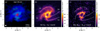 |
Fig. 1 (a) Three-color image of Oph IRS 63, where red, blue, and green represent emissions from the 1.3 mm continuum, SO (56 – 45) (moment 0), and SO2 (83,5 – 82,6) (moment 0), respectively. The synthesized beam is shown in the lower left corner, (b) Moment 0 map of SO (56 – 45) toward Oph IRS 63. The two dashed white ellipses denote the two dust rings of the protoplanetary disk revealed by Segura-Cox et al. (2020). The solid white ellipse represents the SO ring. Four spiral structures (SI to S4) are shown as white curves, (c) Moment 0 map of SO2 (83,5 – 82,6) toward Oph IRS 63. The white ellipse and curves have the same meanings as in panel b. Note that the images shown here represent only a portion of the field of view of the observation and are centered at RA (J2000) = 16h31m35.65s, Dec (J2000) = –24d01m30.1s. |
3 Streamers and accretion shock traced by SO/SO2
3.1 Oph IRS 63
In Oph IRS 63, a low-mass protostar, distinct signatures of accretion shocks have been observed, including ring-like structures and spiral-like streamers in the SO and SO2 emission. These features provide compelling evidence of the presence of shocks at or around the disk-envelope interface during the early stages of star formation. To better understand these shock-related structures, we first examine the detailed morphology and kinematics of the SO emission, beginning with the ring-like component.
3.1.1 SO ring
Among the two observed SO lines (Table 1), only SO (56 – 45) is detected in Oph IRS 63. SO (56 – 45) displays a ring-like structure with multiple spiral-like features (see panels a and b of Fig. 1). The morphology is similar to that revealed by Flores et al. (2023) using the SO (65 – 54) emission at a resolution of 0.3–0.4″. Due to the higher resolution of this study (~0.2″), we are able to observe the SO ring in greater detail and identify that the inner edge of the SO ring resembles an elliptical shape. The elliptical inner boundary of SO has a size comparable to that of the second (outer) dust ring of the protoplanetary disk, as revealed by Segura-Cox et al. (2020) using the ALMA long-baseline data (see also Fig. 1). We fit the ring-like SO emission using an elliptical ring model, following the algorithm described in Appendix A. The azimuthal angle of the major axis (ϕview) and the inclination angle (θview) are fitted to be 53 ± 1° and 40.5 ± 1°, respectively. The fitted value of θview is close to that reported by Segura-Cox et al. (2020) (45°). The small discrepancy may result from deviations from a perfect elliptical shape, or from a possible misalignment between the disk and the SO ring. In this work, we define ϕview = 0 for a structure whose major axis lies in the east-to-west direction, with ϕview increasing as the major axis rotates counterclockwise. Note that in some studies, the position angle (PA) is defined starting from the north direction. During the follow-up fitting, we fixed θview to 45°.
The moment 1 map of SO (Fig. 2a) reveals an hourglass-shaped structure composed of blue- and redshifted components aligned along the major axis of the ring. In the moment 2 map (Fig. 2b), an S-shaped broad-line feature is apparent (see also Fig. B.1). This S-shaped structure corresponds to the southeast-northwest margin of the hourglass seen in the moment 1 map and exhibits a steeper velocity gradient than the southwest-northeast margin. The PV diagram extracted along the S-shaped feature (panel a of Fig. 3) shows distinct velocity components, which we will discuss further in Sect. 5.2.
Here, we focus on analyzing the dynamics of the SO ring itself. We fit the velocity distribution along the ring (panel a of Fig. 2) assuming pure rotation, following Eqs. (D.4) and (D.5). The fitting results are shown in panel b of Fig. 3. The rotational velocity (Vrot) and systemic velocity (Vsys) are fitted to be approximately 2.2 and 3 km s–1, respectively. Assuming Keple-rian rotation at a radius of 65 au, this corresponds to a central mass of ~0.35 M⊙, slightly smaller than the ~0.5 M⊙ reported in the literature (Sect. 2.3).
3.1.2 SO spiral-like streamers of different types
While the ring-like SO structure reveals rotation at the disk-envelope interface (Sect. 3.1.1), additional substructures are present in the form of spiral-like extensions. We now turn to these features, which appear to trace dynamically distinct infalling motions. Four spiral-like structures, denoted as S1 to S4, are identified in the SO emission, with their feet located around the SO ring and their tails extending outward. Among these, S1 to S3 correspond to the three arms reported by Flores et al. (2023), while the S4 structure was not resolved in their work due to slightly lower resolution and sensitivity. In the moment 0 map of SO (56–45) shown in Fig. 1, the western tail and the foot of S4 exhibit an overall S/N exceeding 4, although the emission at the connection between them is weaker (S/N ≲ 3). Given the symmetric distribution of the four feet S1–S4 (Fig. A.1), we consider the presence of S4 to be plausible.
To interpret the origin of the spiral structures, we modeled them as gas streamers undergoing ballistic free-fall toward the disk. Their three-dimensional trajectories were computed and then projected onto the plane of the sky, following the procedure outlined in Appendix C. The free-falling gas, characterized by zero mechanical energy and non-zero specific angular momentum, follows a parabolic trajectory in 3D space. This trajectory is parameterized by the initial polar angle (θ0), azimuthal angle (ϕ0), and centrifugal radius (RC) within the disk coordinate system. For a free-fall stream with a given specific angular momentum J, the centrifugal radius RC represents the radius of an equivalent circular orbit conserving the same angular momentum. Geometrically, RC also corresponds to twice the distance between the focus and the vertex of the parabola. Streams originating from different directions are expected to intersect at or beyond RC, preventing material from freely falling all the way to the vertex of the parabolic path. Additionally, RC equals the distance between the parabola’s focus and its directrix (see Sect. 4.1 for details). When projected onto a two-dimensional plane defined by viewing angles θview and ϕview, the trajectory remains parabolic, although the central star may no longer lie exactly at the focus (see Sect. 4 and Appendix C).
To model the trajectories of the observed spiral-like features, we adopted a simplified, hand-drawn, illustrative approach aimed at qualitatively matching the observed morphology. As a first step, we assessed whether the observed structures can be explained by free-fall streamers confined strictly to the disk mid-plane. According to Eq. (D.3), such midplane-confmed streamers (corresponding to θ0 = π/2) can span an azimuthal angle on the plane of the sky (θproj) of less than 110°. However, some features – such as S1 in Fig. 1 – have Δθproj > 110°, indicating that their trajectories cannot be explained by midplane infall alone. Motivated by this, we fixed the viewing angles, θview and ϕview, to match the inclination and azimuth of the SO ring (and thus the protoplanetary disk; Segura-Cox et al. 2020), and manually adjusted only the model parameters – θ0, ϕ0, and RC – to better reproduce the observed spiral shapes. The uncertainty of θ0 is approximately 10°.
We defined the off-midplane angle as  , which quantifies the deviation of a streamer’s initial direction from the disk midplane. In this convention,
  corresponds to a trajectory lying exactly in the midplane, while
  corresponds to infall along the polar axis. For S1 and S3, we find
  , whereas for S2, it is approximately 10°. The off-midplane angle for S4 is not well constrained; therefore, given the morphological similarity between S1 and S3, we adopt the
  value of S3 for S4. The modeled trajectories are illustrated in Fig. 4, and their parameters are summarized in Table 2.
The above fitting assumes a central stellar mass of 0.35 M⊙ (Sect. 3.1.1). Even after accounting for projection effects, the modeled free-fall velocities are found to be slightly higher than the observed values. To reconcile this discrepancy, we manually scale down the free-fall velocities by a factor of approximately 1.5. This adjustment is justifiable, as the observed velocities correspond to line-center measurements rather than the full velocity span. As demonstrated by Flores et al. (2023), central stellar masses derived from fitting the ridge versus the outer boundary of emission in PV diagrams can differ by a factor of ~3. Furthermore, the free-fall assumption may not be strictly applicable to all streamers, particularly in cases where interactions with the inner envelope alter their dynamics (see Sects. 3.1.4 and 4.2.3).
Based on these results, we classify the spiral-like structures as streamers, supported by several key considerations. First, their large off-midplane angles  indicate significant deviation from the disk midplane. This distinguishes them from typical spiral arms, which are generally confined to the midplane and shaped primarily by disk or inner envelope dynamics (Sect. 4). Second, two distinct SO emission spots are observed at the bases of S1 and S3 – located near the endpoints of the SO ring’s major axis. These spots are clearly resolved in our data (Fig. 1) and may mark the locations where the associated off-midplane streamers appear to intersect the disk surface. Finally, all identified streamers originate from beyond the centrifugal radius (see Sect. 4.1 for the definition of centrifugal radius), where they likely interact with the rotating and infalling inner envelope (see Sect. 3.1.4 for the observational evidence of the inner envelope). These interactions may play an important dynamical role, producing localized heating and chemical enhancement where streamers impact the disk or envelope surface. In the next subsection, we explore such evidence by examining SO2 emission associated with the base of one prominent streamer (Sect. 3.1.3).
To account for the diversity in observed morphologies and infall geometries, we further classify the streamers into two distinct types: in-midplane and off-midplane, corresponding to relatively small (e.g., ≲ 30°) and large (e.g., ≳ 30°) values of  respectively. Additional evidence of both in-midplane and off-midplane streamers is presented for other observational targets in Sect. 3.2. Their differing interactions with the disk and envelope structures are discussed in our modeling framework in Sect. 4.
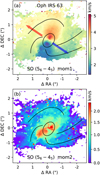 |
Fig. 2 Moment 1 (panel a) and moment 2 (panel b) maps of SO (56 – 45) toward Oph IRS 63. In panel a, the directions of the red and blue outflows (Flores et al. 2023) are indicated by the arrows in the corresponding colors. In panel b, the original moment 2 map has been multiplied by a factor of |

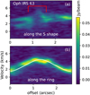 |
Fig. 3 a: PV map of SO along the S-shaped structure observed in the moment maps shown in Fig. 2 (see Fig. B.1 for the implicit marking of the S-shape). The red line marks the location of the SO ring, b: PV map of SO along the sulfur ring (Fig. 1). The white line represents the modeled PV curve of a rotating ring, calculated using Eqs. (D.4) and (D.5). See Sect. 3.1.1 for the fitting results. |
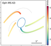 |
Fig. 4 Models of the four spiral-like structures in Oph IRS 63 (Figs. 1 and 2) generated by free-fall streamers, with colors representing the line-of-sight velocity. Model parameters are provided in Table 2 (Sect. 3.1). The dotted gray lines indicate the observed spiral-like structures (Fig. 1), and the blue ellipse marks the SO ring with a major-axis diameter of 1″ (130 au). The color map corresponds to that in panel a of Fig. 2. Velocities are scaled down by a factor of 2 (from the free-fall values) to approximate the observed velocity range (Fig. 2), with justification provided in Sect. 3.1.2. |
3.1.3 SO2 ring and warm spot
All five SO2 lines (Table 1) are detected toward Oph IRS 63 (Figs. 1 and 5). Among these, the SO2 (83,5 – 82,0) transition has the lowest upper-level energy and the highest S/N. Its moment 0 map shows an S/N of approximately 6 (Fig. 1). The emission from SO2 (131,13 – 120,12) (Fig- 5) resembles that of SO2 (83,5 – 82,6) (right panel of Fig. 1), although with a slightly lower S/N of ~5 in its moment 0 map. As with SO, the moment 0 maps of these two SO2 lines reveal a ring-like structure (Figs. 1 and 5). The SO2 ring appears to be comparable in size to, or possibly slightly smaller than, the SO ring. However, due to the current resolution and sensitivity limits, we cannot definitively distinguish between the SO and SO2 rings. We therefore refer to them collectively as the sulfur-oxide rings of Oph IRS 63.
The feet of the streamers are located near the sulfur-oxide ring (Sect. 3.1.2). At these feet, the emission of SO2 (83,5 – 82,0) and SO2 (123,9 – 122,10) is typically enhanced (Figs. 1 and 5). In particular, an emission spot of SO2 (152,14 – 151,15) is only marginally detected at the foot of S3 (see Fig. 5), with a S/N of ~3 in the moment 0 map. However, the average spectrum of SO2 (152,14 – 151,15) at this spot shows a clear detection, with a S/N greater than 5 (Fig. 6). This SO2 spot is spatially close to the SO spot in the same region. The SO2 emission appears more extended than the SO spot and seems to stretch toward the bases of S2 and S3 (Fig. 5), though this interpretation remains tentative due to the relatively low S/N. Notably, the SO2 (152,14 – 151,15) transition has a high upper-level energy of Eu ~ 120 Κ (Table 1), suggesting that the spot at the foot of S3 traces gas that is warmer and/or denser than the average conditions in the sulfur-oxide ring. This may result from the interaction between S3 and the inner envelope or disk near the centrifugal barrier. The large off-midplane angle  of S3 allows it to fall directly onto the midplane in the vicinity of the sulfur-oxide ring (Sect. 4.2.3), potentially generating strong shocks that excite and produce warm SO2 emission. These findings support the interpretation of the spiral-like structures as gas streamers associated with the inner envelope, where their infall motions play a dynamically and chemically significant role near the centrifugal barrier. Our results suggest that the sulfur-oxide ring is likely induced by shocks around the centrifugal barrier, with SO2 serving as a more sensitive tracer of strong shocks than SO (van Gelder et al. 2021).
To further test this interpretation and assess the thermo-chemical state of the gas, we analyzed the SO2 line profiles and constructed a rotational diagram of the warm spot (Fig. 6). The excitation temperature (Tex) and column density (N) of SO2 were determined to be 53 Κ and 3.3 × 1014 cm–2, respectively, using the method described in Appendix E. These results confirm that the SO2 spot is indeed warm, with a gas temperature ≳50K – typical of post-shock molecular gas (Flower & Pineau des Forêts 2015; van Gelder et al. 2021). The SO spectrum at the warm spot exhibits a line width of 1.5 km s–1, a peak brightness temperature of 15 K, and an integrated intensity of 23.4 Κ km s–1. The main uncertainty in the derived column densities stems from the excitation temperature, which is estimated to be accurate within 20% (Fig. 6). Adopting the same Tex as for SO2, the SO column density is calculated to be 5 × 1014 cm–2, corrected for optical depth effects (τ ≲ 0.3; Appendix E). The resulting column density ratio N(SO2)/N(SO) is approximately 0.6 – significantly higher than the value of 0.03 predicted by the fiducial shock model of van Gelder et al. (2021). Both SO and SO2 can be efficiently formed through reactions of atomic S with OH in high-velocity (>4 km s–1) shocks in moderately dense environments (van Gelder et al. 2021). To account for the observed high SO2/SO ratio, a shock velocity exceeding 4 km s–1 is required, which is consistent with the velocity range observed in the SO ring (see the color bar in panel a of Fig. 2). A streamer impacting the centrifugal barrier can generate such a strong shock, enhancing SO2 production. In contrast, streamers that co-rotate with the inner envelope are less likely to experience this level of shock interaction (Sect. 4.2.2). We therefore conclude that the observed SO2 emission at the foot of S3 is likely induced by strong accretion shocks.
Knowing the excitation temperature allows us to estimate the density of the shocked gas. Assuming a warm spot size of 0.2″ (or Lspot ~ 26 au) and a post-shock SO abundance (XSO) of 10–8 (van Gelder et al. 2021), the number density  at the warm spot can be estimated as
 (1)
(1)
Free-fall envelope models – such as the classical CMU model (Ulrich 1976; Cassen & Moosman 1981, with CMU named after the authors’ initials) and the constant-J model (see Sect. 4.2.1 for a brief introduction) – predict a divergent density at the centrifugal radius (RC) due to the neglect of pressure (e.g., Eq. (16)). Given that both the radial thickness of the SO ring and the size of the warm spot are approximately 0.4 RC, we adopted the density at 1.4 ,RC from the constant-J model as a representative value for the inner envelope. Assuming an accretion rate of 10–6 M⊙ yr–1 (Flores et al. 2023), this yields a typical density of ~ 107 cm–3 for the inner envelope – slightly lower than the estimated density at the warm spot (Eq. (1)). This discrepancy may arise from (1) a higher density in the streamers compared to the surrounding envelope, and/or (2) accumulation of material in the post-shock gas.
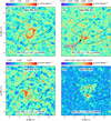 |
Fig. 5 Moment 0 maps of Οph IRS 63 for four SO2 transitions (Table 1). In panel b, the warm SO2 emission spot (Sect. 3.1.3) is highlighted with a dashed ellipse, which is also shown in panel c for comparison. The black ellipse and curves denote the SO ring and the spiral structures, respectively (Fig. 1). For the moment 0 map of the strongest SO2 line, see Fig. 1. |
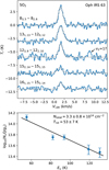 |
Fig. 6 Upper: SO2 spectra of the warm spot in Oph IRS 63, enclosed by a dashed black ellipse in Fig. 5. Lower: rotational diagram of SO2 in the warm spot. |
3.1.4 Inner envelope motion
In addition to the SO rings and spiral-like structures, weak extended SO emission is detected outside the ring. Along the minor axis, the northeast region shows a slight redshift, while the southwest region is slightly blueshifted (panel b of Fig. 2). Because pure rotational motion would produce zero projected velocity along the minor axis, this pattern indicates the presence of both rotational and infalling motions. Given that this extended emission lies primarily outside the centrifugal barrier, we interpret it as tracing the surface of a disk-like envelope confined by an accretion shock. This interpretation is developed based on our combined observational results and is presented in detail in Sect. 4, particularly in Sect. 4.2.2. In other words, we interpret this emission as likely originating from the rotating and infalling inner envelope.
To support the above hypothesis, we first examined the rotational motion of the extended structure. The rotational and infalling velocity components may be coupled; however, the projection of the infalling velocity component along the major axis of the disk and inner envelope is expected to be zero (assuming negligible envelope flare). Therefore, the PV map of SO along the major axis of the SO ring (panel a of Fig. 7) primarily reflects the rotational velocity component. The rotational velocity of the inner envelope is expected to follow a power-law with radius, characterized by an index β that can range from 0 (free fall with zero angular momentum) to –1/2 (Keplerian rotation), or even –1 (free fall with conserved angular momentum). This framework is further detailed in Eq. (24) and Sect. 4.2.2. If the motion of the post-shock surface traced by the extended SO emission is fully governed by the underlying gas flows, one would anticipate a velocity index close to β = –1. However, given the current sensitivity, we cannot conclusively distinguish between β = –1 and β = –1/2. Thus, while both pure rotational and rotating–infalling motions remain consistent with the velocity distribution along the major axis, our combined kinematic analysis confirms the presence of infalling motion in the extended structure.
Furthermore, we modeled the 2D distribution of the projected velocity for a rotating and infalling inner envelope (see panel b of Fig. 7), using Eqs. (25) and (24). The rotation follows a power-law with an index (β) of –1, while the infall velocity is fixed. We adjusted the ratio of these velocities to match the observations. The modeled velocity distribution reproduces key features of the observed data (Fig. 2), including: (1) the slight offset between the major axis of the SO ring (represented by the blank ellipse in panel b of Fig. 7) and the symmetry axis of the moment-1 map; and (2) the S-shaped structure in the moment-1 map, extending from the lower left to the upper right of panel b in Fig. 7 (see panel a of Fig. 2 for the observed S-shape). This confirms that the extended SO emission outside the ring can be explained by emission from a disk-like inner envelope, potentially originating from its surface, with its rotating–infalling motion tracing the continuation of the free-fall streams with non-zero angular momentum.
These modeling results provide a physical basis for interpreting the structure and dynamics of the inner envelope, which plays a critical role in mediating accretion from large scales. Building on this, we now turn to the interaction between the streamers and the envelope. The inner envelope offers a valuable window into accretion processes near the disk and the behavior of gas streamers. Conceptually, off-midplane streamers are expected to have a strong dynamical impact on the envelope at their collision sites, while in-midplane streamers may gradually merge with the inner envelope and effectively serve as part of it. This distinction provides a qualitative framework for understanding the varying shock activity associated with different types of streamers. A more detailed discussion of these interactions is developed in the context of the disk–envelope framework in Sects. 4.2.2 and 4.2.3.
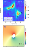 |
Fig. 7 a: PV map of SO in Oph IRS 63 along the major axis of the SO ring marked in Fig. 1. The dashed and dotted black lines represent the fits to the velocity distribution of Vϕ with power-law indices of –1 (the free-fall case with non-zero angular momentum) and –0.5 (the Keplerian case), respectively (see Sect. 4.2.2 for details), b: modeled velocity of an inner disk-like envelope (in a simplified 2D version) with its projection parameters (θview and ϕview) identical to those of Oph IRS 63. The radial (υr) and azimuthal (Vϕ) velocities are given by the formulas in the legend, following Eqs. (25) and (24), which describe the possible motion of disk-like inner envelopes (see Sect. 4.2.2 for details). Note that the model is scale-free, and we have adjusted the velocity range and central velocity for better agreement with the observations (panel a of Fig. 2). |
3.1.5 Tentative features in the SO2 line profiles
At the warm spot, the SO2 spectra with higher Eu appear to be more blueward-skewed (Fig. 6). SO2 (152,14 – 151,15) exhibits the most prominent characteristic with a blue shoulder, albeit with a S/N of only ~2.5. We tentatively interpret this as evidence that S3 has a large  and impacts the midplane with a blueshifted velocity (see Fig. 4). Near the emission line of SO2 (123,9 – 122,10), there is a weak (2σ) line feature at ~8.5 km s–1 with respect to the rest frequency of SO2 (123,9 – 122,10). This feature has a frequency close to the rest frequency of the transition 263,23 – 254,22 of SO2 υ2 = 1. This transition has a very high Eu value of >1117 K. The ground-level energy of SO2 υ2 = 1 is ~745 Κ (Müller & Brünken 2005), and this transition has an Eu of 372 Κ with respect to the ground level of SO2 υ2 = 1. If the emission line of this transition has a velocity shift similar to that of SO2 (123,9 – 122,10), its peak should appear at ~10 km s–1. The location of this line feature on the velocity axis is consistent with the blueward skewing trend observed for the high-Eu lines of SO2 at the warm spot. Considering that the Tex given by the rotational diagram of SO2 (Fig. 6) is only a few tens of Kelvin, this transition would be unlikely to be excited if it originates from the same gas component traced by the relatively low-Eu lines. One possibility is the presence of a hotter gas component that allows for the excitation of vibrational states of SO2 υ2 = 1, via processes such as infrared pumping (van Gelder et al. 2024). While we cannot entirely rule out this scenario, we consider it more likely that this line feature is a random observational spike, given its low S/N in Oph IRS 63 and the lack of a corresponding detection in DK Cha, an object with much stronger emission of sulfur-bearing molecules and warmer SO2 spots (Sect. 3.2).
3.2 DK Cha
While clear signatures of accretion shocks, such as ringlike features and spiral streamers in SO and SO2 emission, were observed in Oph IRS 63, the situation for DK Cha, an intermediate-mass protostar, is less straightforward. Nevertheless, its likely more face-on orientation and the limited resolution of the available data still provide valuable insights into how shock features might manifest in a different mass regime.
3.2.1 Inclination angle of the disk continuum
There are no ALMA long-baseline data (with a beam resolution better than 0.1″) available for this object in the archive. Fig. 8 shows the moment maps of SO and SO2 for DK Cha, overlaid with its dust continuum at a resolution of ~0.2″. Although our data do not fully resolve the disk, the nearly round morphology of the continuum emission suggests that DK Cha has a nearly face-on disk. The 2D Gaussian fitting of the continuum gives a major-axis FWHM of 0.44″ ± 0.01″, a minor-axis FWHM of 0.38″ ± 0.11″, and a PA (ϕview) of 43° ± 10°. The values for the synthesis beam are 0.22″, 0.15″, and 65°, respectively. The beam-deconvolved4 major-to-minor axis ratio of the continuum emission gives a θview of ~20°. This result is consistent with the findings from the analysis of the multi-cone outflows of DK Cha by Harada et al. (2023), who reported a θview of 19°. The [S II] 6731 Å data from VLT MUSE (Sect. 2.1.2) show an outflow lobe in the north-east direction of DK Cha (panel a of Fig. 8). This is likely the blueshifted lobe, while the redshifted one is not visible due to extinction. This confirms that the disk of DK Cha is nearly face-on with a small θview Therefore, we adopt a θview of 20° for the disk of DK Cha in this work. Similar to Oph IRS 63, the emission of SO and SO2 is absent in the disk region of DK Cha, as traced by the dust continuum. The nearly face-on geometry of DK Cha and the absence of SO and SO2 emission within the disk region, similar to Oph IRS 63, suggest that this chemical differentiation is intrinsic rather than a projection effect, reinforcing the importance of geometry when interpreting molecular tracers in protostellar environments.
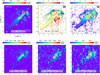 |
Fig. 8 Moment maps of SO and SO2 for DK Cha. The transition quantum labels are provided at the bottom of each panel, and the beam is indicated in the lower left corner of the first panel. In panel a, the black contours represent the ALMA continuum emission at levels of [0.01, 0.5, 0.9] times the peak value (0.16 Jy beam–1 ). In the other panels, only the 0.5 times the peak value contour of the ALMA continuum is shown. The white contours in the first panel outline the north-east lobe of the outflow, as traced by [S II] 6731 Å using VLT/MUSE. This outflow has been smoothed to match the resolution of the ALMA data. The white contour levels are [0.3, 0.5, 0.7] times the peak value. Substructures identified in the moment 0 map of SO are labeled in the upper left panel, with three streamers (S1 to S3) marked by black curves. For an illustration of additional substructures, their names, and connections, refer to the schematic image in Fig. 12. As in panel b of Fig. 2, the moment 2 map of SO in this figure has been multiplied by a factor of |

3.2.2 Streamers and warm spots
Building on the clear identification of spiral-like streamers in Oph IRS 63, we detect analogous features in DK Cha, although with differing morphologies and S/Ns that likely reflect the influence of its more face-on orientation and varying shock activity (Fig. 8). Three spiral-like structures can be identified on the moment 0 map of SO (S1–S3; Fig. 8). The stronger heads of S1 and S2 have S/Ns greater than 10, while the weaker tails of S1–S3 have S/Ns of approximately 5. As is observed in Oph IRS 63, we interpret these as accretion streamers of DK Cha. It is evident that the southeast tail of S2 exhibits very narrow line widths (ΔV ~ 0.5 km s–1; Fig. 9). The line width of S2 increases dramatically when it intersects with P1, a broad-line (FWHM of ~3 km s–1) and SO-bright segment with a projected length of ~300 au. P1 is also bright in SO2 emission (panels d–f of Fig. 8). The inner end of P1 is located at the boundary of the disk traced by the dust continuum. There is no obvious velocity gradient along S2 and P1, which may be due to projection effects, given that DK Cha is nearly face-on and S2 lies along the major axis in the plane of the sky. In addition to S2, a short streamer, S3, is also connected to P1. The intersection between S3 and P1 produces a compact spot (with a size comparable to the beam), which is very broad in line width (FWHM of ~4 km s–1). Below, this spot is denoted as S3 ⊥ P1. We interpret that both S2 and S3 are falling onto the inner envelope: the falling gas forms the streamer P1, and P1 continuously feeds material to the central disk. A warm spot is created when S3 hits P1. P1 continuously endures shocks as it passes through the inner disk, leading to a long segment of emission of SO and SO2 (Sect. 4.2.3).
S1, the north streamer, is connected to a compact spot (denoted as P2 in the PV maps; Fig. 8), which has both emission of SO and SO2. P2 has a line width comparable to that of S3 ⊥ P1. The excitation temperatures of SO2 of the two spots (P2, and S3 ⊥ P1) are calculated through drawing the rotation diagrams of SO2 (Fig. 10). P2 has a higher excitation temperature of SO2 than S3 ⊥ P1 (Sect. 3.2.3). We interpret that S1 is a off-midplane streamer (Sect. 4.2.3), and it directly hits the inner envelope near the centrifugal barrier, creating the hot spot P2. The warm spots in DK Cha are generally hotter than those in Oph IRS 63, which is expected due to DK Cha’s more massive central star. Furthermore, DK Cha’s higher gas density, compared to Oph IRS 63, aids in detecting the high-Eu lines.
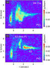 |
Fig. 9 PV maps along the two dotted lines in panel a of Fig. 8. Panels a and b correspond to the northern and southern lines in Fig. 8, respectively. Several gas components identified in Fig. 8 are visible in the PV maps, and are labeled accordingly. |
3.2.3 A hot SO2 spot of DK Cha?
Compared to the warm spot of S3 ⊥ P1, which has Tex ~ 70 K, the spot P2 exhibits an even higher temperature of Tex > 100 Κ (Fig. 10). Therefore, P2 can be considered a hot spot. We examined the spectrum of SO2 161,15 – 152,14, which has the highest Eu (131 K) among the observed lines toward DK Cha at P1 (Fig. B.2), and it shows a S/N higher than 5, confirming that the high fitted temperature is not caused by noise or spikes. The temperature difference between the two spots can be explained by the differences in θview and the specific angular momentum of the streamers that produce them. S1 directly interacts with the midplane at P2, which is significantly closer to the center of mass compared to S3 ⊥ P1. Because S1 is off the midplane, it experiences less deceleration from the inner envelope before the strong shock occurs (Sect. 4.2.3), leading to a hotter spot at P2. The presence of multiple streamers interacting with the inner envelope and producing warm spots and segments – characterized by excitation temperatures notably higher than those in Oph IRS 63 – highlights the influence of stellar mass and polar angle in governing the nature and detectability of shock signatures.
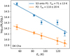 |
Fig. 10 Rotation diagrams of the SO2 emission of the two warm spots (P2 and S3 ⊥ P1) of DK Cha (Fig. 8). The emission is extracted at the positions marked by black crosses in Fig. 8. |
3.2.4 Streamers traced from archived CO data
Consistent with the SO and SO2 maps, archival CO (2–1) observations provide additional – albeit lower-resolution – confirmation of the streamer structures (Fig. 11). Two of the three streamers identified in SO (S1 and S2; Fig. 8) are marginally visible in the moment 0 map of the archived CO (2–1) data. To reduce contamination from outflows, we integrated a narrow velocity interval (1–5 km s–1) around DK Cha’s systemic velocity (~3 km s–1; Kristensen et al. 2012). The CO emission generally lies on the convex sides of the SO-traced streamers, suggesting outward forces acting upon them (Sect. 4). Within the disk region traced by the ALMA continuum, CO (2-1) spectra show strong absorption near the systemic velocity. Moreover, the CO data have a lower spatial resolution than the SO data (Sect. 2), so the moment 1 map of CO (panel b of Fig. 11) only roughly traces the disk’s velocity gradient (Sect. 3.2.5). A bright CO arc is visible at the southeastern disk margin, potentially marking the centrifugal barrier or the interaction between segment P1 and the inner envelope (Figs. 8 and 12), although contamination from low-velocity outflow components cannot be excluded (Harada et al. 2023). Together, the CO data offer important complementary insights into the dynamics and external influences governing the infalling gas streams.
3.2.5 Discussion of the direction of rotation
Extended SO emission features P3 and P4 (Fig. 8) appear at blueshifted and redshifted velocities, respectively, but their origins are challenging to interpret (Fig. 12). One possibility is that P4 represents the inner part of a streamer similar to S2 and S3, infalling onto the inner envelope rather than onto Pl. P3 might simply be part of P2. Alternatively, these features could trace warm molecular gas influenced by outflows (van Kempen et al. 2006), or be shaped by the disk’s rotation.
Despite the wealth of spatial and spectral information, the exact rotational direction of DK Cha’s disk remains uncertain. The morphology of S1 and the velocities observed in P1 and P2 suggest that DK Cha’s disk rotates clockwise (Fig. 12), a scenario supported by the velocity distribution of CO (2–1) within the disk region (Fig. 11). However, this interpretation does not fully explain the morphology of S2. The radial velocity gradient of S2 (panel b of Fig. 8) differs from that expected in a simple rotational scenario, which may point to additional factors influencing its trajectory. One possibility – though speculative – is that S2 is affected by external pressure on larger scales (on the order of thousands of astronomical units), perhaps from east to west, leading to reduced specific angular momentum. The angular momentum of S2 appears to decrease further as the gas enters P1, likely due to interactions between P1 and the inner envelope (Sects. 4.2.2 and 4.2.3). Consequently, P1 moves inward toward the central mass with low specific angular momentum, and continuous shocks are expected as it propagates through the inner envelope. This scenario may explain the linear morphology and broad SO and SO2 emission observed along Pl. A schematic illustrating the connections between these streamers and features in DK Cha is provided in Fig. 12.
Previous observations have revealed multi-cone outflows in DK Cha with highly complex morphologies (Harada et al. 2023). These intricate dynamical interactions, combined with external pressure and the multi-cone outflow structure, likely reflect the effects of variable angular momentum accretion and intermittent shock-driven phenomena, consistent with scenarios proposed for other protostellar systems (e.g., Zhu et al. 2009; Nony et al. 2020).
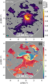 |
Fig. 11 Moment maps of CO (2-1) for DK Cha. Only data within the velocity interval of 0–5 km s–1 were utilized to calculate the moment maps (Sect. 3.2.1). Velocity channels with intensities exceeding 3σ are included in the moment map calculation. In each panel, data outside the dashed white circle have been masked out. White curves represent the streamers identified from the SO emission (Fig. 8). The black contours denote the ALMA continuum, as shown in panel a of Fig. 8. The two ALMA observations were conducted in 2015 and 2023, respectively (Sect. 2). Position shifts due to proper motion and/or possible phase calibration uncertainties have been corrected by cross-matching their continuum peaks, determined via 2D Gaussian fitting. In panel a, the synthesis beams of the CO and SO data are represented by the black and cyan ellipses at the lower left corner, respectively. |
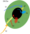 |
Fig. 12 Schematic image of DK Cha based on its emission of SO and SO2 (Fig. 8). The major gas components that can be seen from the observed data (Fig. 8) are labeled. The black ellipse marks the disk traced by continuum that cannot be fully resolved. The direction of rotation is unknown, and we suggest a clockwise rotation based on the velocity distributions along the streamers and near the disk traced by SO and CO (2-1) (Figs. 8 and 11; see also Sect. 3.2.5). The green ellipse is the assumed disk-like inner envelope, which has strong interaction with the streamers that fall onto it (S1, S2, and S3). The interaction contributes to the enhancement of SO/SO2 emission on the segment (P1) and spot (P2) at the inner envelope (Sect. 3.2). |
3.3 L 1527
In contrast to Oph IRS 63 and DK Cha, L1527, an edge-on Class 0 protostar, provides a different perspective on accretion shocks. The presence of accretion shocks in L1527, as traced by SO and SO2 emission, offers valuable insights into how these features manifest in an edge-on system, shedding light on the dynamics of accretion in protostellar disks and envelopes.
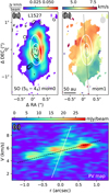 |
Fig. 13 a–b: moment maps of SO of L1527. The white contours represent the continuum emission, with levels of [0.1, 0.5, 0.9] times the peak value. The black contours represent the integrated intensity of SO2 163,13 – 162,14, with levels of [8, 11] Jy beam–1 km s–1. The moment 0 map SO2 is shown in Fig. B.3. In panel b, the beam is shown in the upper right corner by a gray ellipse, c: PV map of SO along the dotted black line in panel b. The solid white and dashed black lines denote the two linear structures on the PV map. |
3.3.1 Parallel slabs of SO
The SO emission from L1527 measured in this work (Fig. 13) reveals two parallel slabs, nearly identical to those observed in different SO transitions in Sakai et al. (2014, 2017). This supports the interpretation that SO emission arises from the surface of a disk or disk-like structure (see also Sects. 3.1.4 and 4.2.2). We only cover one SO2 transition for L1527 (Table 1), which is marginally detected (Fig. B.3). Between the parallel slabs of SO, there is a compact region, approximately 50 au in size, which exhibits SO2 163,13 – 162,14 emission (Eu = 148 K), as is shown by the black contours in Fig. 13 (see also Fig. B.3). Due to the limited data (only one transition), the temperature of the SO2−emitting region cannot be well constrained. The SO2 emission also appears to show two parallel slabs, but the low S/N prevents further analysis. Given that the SO2 transition has a high excitation energy (Eu ~ 150 K, Table 1), it likely traces a region that is warmer compared to the average temperature of the SO emission region.
3.3.2 Two rings of SO at the disk scale
The PV map of SO along the major axis of L1527 (panel c of Fig. 13) reveals an X-shaped morphology composed of two linear strips, each showing a distinct velocity gradient. Note that each linear strip in the PV map corresponds to an edge-on rotating ring, since both the projected velocity (υproj) and projected distance (rproj) exhibit sinusoidal dependence on the azimuthal angle ϕ:
 (2)
(2)
The longer and brighter strip with the smaller velocity gradient corresponds to the outer ring (the parallel slab), which has been previously reported and interpreted as the centrifugal barrier of the envelope (Sakai et al. 2014, 2017). In contrast, the fainter strip exhibits a much steeper velocity gradient (Fig. 13) and likely traces a newly identified inner ring of SO emission located inside the centrifugal barrier. We refer to these features as the outer and inner rings, respectively.
The radii of the two SO rings inferred from the PV map are approximately rout ~ 150 au (or ~1″) for the outer ring and rin ~ 35 au for the inner ring. The inner SO ring has a size comparable to the SO2 emission region (Fig. 13). The corresponding velocity gradients observed on the PV map are  km s–1 arcsec–1 and
  km s–1 arcsec–1, respectively. These values approximately obey the relation
 (3)
(3)
suggesting that both rings are in Keplerian rotation. This follows because, for Keplerian motion, the rotational velocity satisfies
 (4)
(4)
and the corresponding velocity gradient scales as
 (5)
(5)
Using Equation (4), the central mass of L1527 is estimated to be ~0.5 M⊙, consistent with the recent dynamical mass measurement (including the star and disk) by van’t Hoff et al. (2023) (see Sect. 2.3).
A similarly steep linear structure was also observed in the PV map of H2CO in L1527, corresponding to a radius of ~25 au (van’t Hoff et al. 2023), which is consistent with the inner SO ring found in this work. That study interpreted the H2CO structure as marking the snow line of H2CO, located at a temperature of ~70 K. By analogy, the inner SO ring may represent the snow line of SO. The sublimation temperature of a molecular species depends on its binding energy, which remains uncertain (McElroy et al. 2013; Penteado et al. 2017). According to the UMIST database (McElroy et al. 2013), the binding energy of SO is 2600 K, which is somewhat higher than that of H2CO (2050 K), though other studies suggest a lower SO binding energy of ~1800 Κ (Penteado et al. 2017). This implies that the inner SO ring may indeed trace the SO snow line. In this interpretation, SO is initially enhanced at the centrifugal barrier (outer ring), then depleted or destroyed within the outer disk, and re-enhanced near the snow line (inner ring). Similarly, SO2 is also enhanced in the vicinity of the inner SO ring.
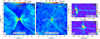 |
Fig. 14 a: moment 0 map of CO (2-1) of L1527. The integration range is 0.8–11.6 km s–1. The beam size is shown as black ellipse at the lower left corner. The black lines mark the boundaries of CO outflows, b: moment 0 map of SO, cleaned using the natural weighting (Sect. 2.1.1). To improve the S/N, we have further smoothed the map to a beam size of 0.7″, as indicated by the black ellipse in the lower left corner. The white arrows mark the outflows. The black lines have the same meaning as in the left panel, and are denoted as SW, SE, NW and NE, accordingly to their locations, c and d: PV maps of SO along the outflow boundaries marked in the lower right corners. The dotted white lines represent the fitting results of the trajectories of free-fall streams in PV space (Sect. 3.3.3). See Figs. El and F.2 for the typical spectra of SO along the outflow boundaries. |
3.3.3 Infalling layer of SO along the outflow boundary
We now turn to the large-scale SO emission. No obvious streamers of SO are visible in the data cube cleaned using the Briggs robust = 0.5 weighting scheme (Sect. 2.1.1). Compared to this weighting scheme, the natural weighting (robust = 2) assigns equal weight to all samples, resulting in lower noise levels and a larger synthesized beam. Thus, the natural weighting enhances the S/N of large-scale emission. We examined the data cube of L1527, cleaned using natural weighting, to search for large-scale SO structures. Surprisingly, linear SO emission structures, referred to as SO strips, are visible along the boundaries of CO outflows (Fig. 14). The most prominent SO strip lies along the southwestern (SW) outflow boundary, extending over 12″ (1700 au) from the central protostar, with a S/N (at the emission peak) exceeding 5 in the moment 0 map. The emission along the SW boundary is even more pronounced in the PV map, where the S/N exceeds 7. The SO spectrum stacked along the SW direction exhibits a very narrow linewidth of approximately 0.44 km s–1 (see Appendix F for details), confirming that the SO emission along the outflow boundaries is only partially resolved spectrally. Along the northwestern (NW) and southeastern (SE) outflow boundaries, SO emission is only marginally detected in the moment 0 map (panel b of Fig. 14). However, in the PV map (panel d of Fig. 14), narrow-line SO emission is clearly observed along these boundaries, with S/Ns of ~5.
A notable feature of the SO strips, particularly along the SW boundary, is that the SO emission peak is spatially offset from the CO emission peak, lying on the convex (outer) side of the outflow boundaries. To quantify this spatial offset between the two tracers, we present the averaged transverse emission profiles of SO and CO along the outflow boundaries in Fig. 15. For the SW boundary, a significant offset is found between the Gaussian fits of the SO and CO profiles, with a t-statistic exceeding 15 (Table F.I), indicating a highly significant separation. The SO emission is shifted by approximately 0.7″ ± 0.01″ relative to the CO emission in the transverse direction, suggesting that SO traces the convex side of the hourglass-shaped CO cavity walls. The FWHMs of the Gaussian fits are 1.3 ± 0.1″ for SO and 0.9 ± 0.1″ for CO. Note that the CO and SO images (with natural weighting) have similar beam sizes of 0.32″ and 0.35″, respectively. The narrow transverse profiles confirm the presence of well-defined strips in the moment 0 maps, with the CO boundary appearing sharper than the SO strip. Similar spatial offsets between CO and SO are also observed along the NE and NW boundaries (Fig. 15). Since the transverse directions differ for each boundary, these systematic offsets cannot be attributed to image misalignment between the CO and SO data. This supports the interpretation that the SO emission originates from a conical layer that is either geometrically thicker or located farther from the outflow axis than the CO-emitting surface.
The SO spectra along the strips (outflow boundaries) exhibit central velocities close to the systemic velocity at large scales (6 km s–1), with their velocity offset (relative to the systemic velocity) increasing significantly as the distance from the central protostar decreases (Fig. 14). This behavior suggests that the SO layer may be undergoing infalling motion rather than outflowing. To test this hypothesis, we modeled the strips in the PV maps using free-fall trajectories, following a similar approach to that in Fig. 4 (see details in Appendix C). In the model, we adopt a central mass of M★ = 0.5 M⊙ (Sect. 3.3.2), a centrifugal barrier radius of RC = 1″, and viewing angles θview = 90°, ϕview = 90°, with initial trajectory angles θ0 = 45° and ϕ0 = 0°. Remarkably, the free-fall trajectories reproduce the observed strips very well (panels c and d of Fig. 14). From the PV maps, it is evident that the southern strips along SE and SW do not directly connect to the southern blue part of the SO ring, but rather to its northern part. Similarly, the northern strip along NW appears connected to the southern blue part of the SO ring. This supports the interpretation that the SO strips do not move along straight paths but instead follow curved (possibly parabolic) trajectories wrapping around the outflow cone as they move inward.
Observations of protostars such as HH 211 and IRAS 16293–2422 Al reveal that SO emission can exhibit velocity gradients perpendicular to the outflow axes, which have been interpreted as signatures of twisted magnetic fields (Lee et al. 2021; Oya et al. 2021). Due to the limited S/N in our data, we are unable to place meaningful constraints on any velocity gradient perpendicular to the outflow axis in L1527.
Based on the preceding results, we propose the presence of a mildly shocked, conical SO-emitting layer undergoing downward-spiraling infall, which warps the outflow cavity. The observed SO emission pattern may result from interactions between the outflow and the infalling envelope, suggesting that angular momentum transfer from the outflow to the envelope is non-negligible (Sect. 4.2.1). We interpret the infalling SO layer as tracing the surface of the outer envelope on large scales (from hundreds of astronomical units to over a thousand). An increase in angular momentum leads to an outward expansion of the centrifugal radius. As a result, on smaller scales (from hundreds of astronomical units to several thousand), the outflow boundary does not necessarily make direct contact with the inner envelope (Sect. 4.2.1).
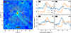 |
Fig. 15 a: same as Fig. 14 but with gray arrows indicating the transverse directions along the outflow boundaries used for extracting radial profiles. The direction of each arrow denotes the positive offset direction, pointing toward the inner regions of the outflow cavities, b–d: averaged emission profiles along the transverse directions for the NE, NW, SE, and SW boundaries (corresponding to panel a). The SO emission is extracted from the image cleaned with natural weighting (without the additional smoothing applied in panel a). For comparison, the CO emission (orange) is divided by a factor of 30 and plotted alongside the SO emission (blue). Dotted lines show the corresponding fits using a Gaussian plus linear function. |
4 Shock confined outer and inner envelopes?
In the previous sections, we have shown that SO and SO2 emissions primarily trace shocks located near the centrifugal barrier and at the bases of infalling gas streamers. These observational features indicate that shocks play a significant role in shaping both the envelope structures and the disk-envelope interface. Furthermore, the spatial and kinematic patterns of SO emission near the outflow boundaries suggest possible interactions between the infalling envelope and the outflow. Although this evidence remains tentative, such interactions may contribute to compressing the outer envelope and consequently influence the motions of the inner envelope. The interaction between streams (or streamers) and the envelope (or disk) serves as a key factor in the patterns of shock-related emission. Motivated by these observational insights, we constructed a self-consistent model of the disk-envelope system and the streamers to explore these possibilities further and to better understand the physical mechanisms driving the observed features.
4.1 CMU model
We begin by considering the classical “CMU” model of a proto-stellar envelope (Ulrich 1976; Cassen & Moosman 1981). In this model, the gas moves in free fall with zero total energy (the sum of kinetic and gravitational potential energy). For a gas stream initially infalling with a polar angle, θ0 (measured from the system’s rotation axis, which is typically defined by the angular momentum of the protostar and its surroundings), the specific angular momentum is given by
 (6)
(6)
Here, θ0 is the initial polar angle of the gas trajectory relative to the rotation axis. By convention, θ0 = 0 corresponds to the rotation axis (pole), and θ0 = π/2 corresponds to the midplane (equator). At the midplane, j(π/2) = 1, meaning the specific angular momentum is largest there.
Ignoring gas pressure, the gas stream follows a parabolic trajectory. The radius of the centrifugal barrier – defined as the distance from the focus to where the parabolic path crosses the midplane – is
 (7)
(7)
where
 (8)
(8)
This  is the centrifugal barrier radius for gas falling exactly in the midplane.
Under the gravity of the central star (ignoring the envelope’s self-gravity), the parabolic trajectory is described by (Ulrich 1976)
 (9)
(9)
where r and θ are the radius and polar angle at a given point along the streamline.
The radial infall velocity (velocity component along r) is (Cassen & Moosman 1981)
 (10)
(10)
Although υr depends on r, θ0, and θ, substituting Equation (9) removes the explicit dependence on θ.
Assuming the accretion rate at large distances is spherically symmetric, mass conservation implies that the gas density can be expressed as (Cassen & Moosman 1981)
 (11)
(11)
The original CMU model assumes
 (12)
(12)
which leads to
 (13)
(13)
The density depends on both the radius, r, and polar angle, θ (see panel a of Fig. 16). Taking  as the disk radius, the mass infall rate from the envelope onto the disk within radius
  is
is
 (14)
(14)
Equation (14) leads to half of the envelope’s mass falling onto the disk within  . However, this conflicts with observations showing that shock tracers such as SO and SO2 are lacking in the central disk region (Sect. 3). One possible explanation is that stellar radiation destroys these molecules during infall. But since the SO/SO2 snow line is expected to lie very close to the star in low-mass protostars (see Sect. 3.3 and references therein), radiation may not fully destroy these species. A more likely explanation is that some mechanism prevents envelope gas from directly falling onto the inner disk regions.
4.2 Constant-J case
The model of Ulrich (1976) requires a gas stream with a small θ0 (initially from near the pole) to have very little angular momentum. This may not hold under the influence of stellar feedback. Outflows and jets are common in protostars and are believed to clear the polar region, forming a cavity (e.g., Bally 2016; Liang et al. 2020). The cavity would exert continuous pressure on the gas stream originating near the pole during the early stages of accretion, efficiently increasing the stream’s angular momentum. This is supported by the infalling layers of SO closely tracing the outer edges of the CO outflow boundaries (see the example of L1527 in Sect. 3.3.3). Thus, j(θ0) is not necessarily required to be an increasing function of θ0. Note that a stream with a larger j(θ0) will have a larger RC (Eq. (7)). If j(θ0) is a decreasing function of θ0, the streamlines from different θ0 values will interact with each other before reaching their centrifugal barriers. However, considering that the inner pressure of the outflow could influence the system at a large scale (e.g., thousands of astronomical units), there is enough time for the pressure gradient within the envelope to adjust the angular momentum of different streams. Therefore, we adopt a constant-J case with
 (15)
(15)
and denote it as the constant-J model.
4.2.1 Hard-surface envelope by stellar feedback
In the constant-J model, the centrifugal barrier radius, RC, is constant and does not depend on the initial polar angle, θ0. Ignoring pressure effects, gas streams originating from different θ0 values will converge and interact at the same radius, RC (Eq. (7)). The density of the infalling gas can then be expressed as
 (16)
(16)
and using Eqs. (9) and (15), one obtains the relation
 (17)
(17)
Substituting Eq. (17) into Eq. (16) gives a simplified expression for the density:
 (18)
(18)
This is equivalent to Eq. (11) when a constant RC is assumed. Note that in the constant-J model, ρ explicitly depends only on r and not on θ or θ0. Physically, this implies that at a given radius, r, the infalling gas is uniformly compressed in the polar angle (θ) direction for  , while the density sharply drops to zero for
  . This discontinuity defines a “hard surface” for the envelope (panel b of Fig. 16). Note that external pressure sources, such as outflows, may only become significant at large radii. At smaller radii, the envelope surface does not need to be in direct contact with or confined by stellar feedback. Recent near-infrared JWST observations support the presence of an empty region between the outflow cavity and the inner envelope surface (e.g., Harsono et al. 2023).
Similarly, substituting Eq. (17) into Eq. (10) yields
 (19)
(19)
Thus, the radial infall velocity, υr, also becomes independent of both θ and θ0. Therefore, in the constant-J model, both υr and ρ explicitly depend only on the radius, r (see panel b of Fig. 16). For a stream lying in the midplane, the azimuthal velocity is given by
 (20)
(20)
where υr is given by Eqs. (10) and (17).
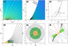 |
Fig. 16 a: density distribution of the Ulrich (1976) model of the envelope. The black lines are the streamlines, b: same as the first panel but for the constant-J case (Sect. 4.2.1). c: streamline for θ0 = 0 in the constant-J case. Note that ρ depends only on r in the colored region, d: streamlines altered by disk-like inner envelope. The green area represents the disk-like envelope supported by thermal pressure and confined by shocks at the surface (Sect. 4.2.2). The orange area shows the schematic diagram of a Keplerian disk within the centrifugal barrier at RC, with a flare index of 1.3 (e.g., Chiang & Goldreich 1997). The vertical orange-red bar shows the head-on strong shocks at the centrifugal barrier (redder color means stronger shocks). The horizontal blue bar roughly represents the shocked surface of the envelope due to oblique flows, e: streamlines in the envelope viewed from the pole. The gray and yellow regions represent the outer and inner envelopes, respectively. The solid blue line depicts the free-fall parabolic trajectory in the midplane. The dotted and dashed lines are the pressure-modified trajectories in the midplane and on the surface of the inner envelope, respectively, f: schematic map in edge-on view. The gray, green, and orange regions are the outer envelope, disk-like envelope, and the disk, respectively. The black strips are the near-middle-plane (lower left) and off-midplane (upper right) streamers. The arrows indicate the outflows. The red dots highlight the shocked surfaces of the disk-like envelopes. |
4.2.2 Disk-like inner envelope confined by accretion shocks
The model above considers only the streams in free fall. As r approaches the centrifugal barrier, the density increases drastically. When the streams reach the centrifugal barrier, shocks occur. A pressure gradient will develop due to the accumulation of material and the rise in temperature. As a result, the inner region of the envelope will swell (panel d of Fig. 16).
For the stream with θ0 = 0 (initially from the pole), when it enters the swell-up region, it will experience two types of decelerating forces: one from the ram pressure and the other from the thermal pressure gradient. The ram pressure force is aligned with the direction of gas motion (–Vinfall). The thermal pressure gradient, on the other hand, is directed along r, since ρ is constant as a function of θ at a fixed r (see Sect. 4.2.1). We denote h = z(r, θ) = r cos(θ) as the height of the stream above the midplane, and υh as the velocity of the stream approaching the midplane. According to the geometric properties of a parabola (panel c of Fig. 16), at a given point on the streamline (r, θ),
 (21)
(21)
and
 (22)
(22)
The ram pressure will decelerate both υr and υh equally, allowing the stream to continue moving toward the centrifugal barrier. In contrast, the thermal pressure gradient exerts a stronger decelerating effect on υr than on υh, causing the stream to fall onto the midplane before reaching the centrifugal barrier. Shocks will occur between the stream and the swell-up region if the residual of υh (denoted as  ),
),
 (23)
(23)
exceeds the sound speed.
Confined in the h direction by shocks at its surface, the swell-up region will then be shaped into a flattened disk-like envelope (as qualitatively represented by the green area in panel d of Fig. 16). The detailed distribution of the velocity of the disklike inner envelope is complex. For simplicity, we propose the following for a stream in the midplane:
 (24)
(24)
 (25)
(25)
That is, υr is constrained to a constant value (with a power-law index β = 0), while υϕ remains largely unaffected compared to Eq. (20). This results in a rotating-and-infalling disk-like inner envelope, with a steeper decrease in υϕ (β = –1) as r increases, compared to Keplerian motion (β = –1/2). The surface of the disk-like inner envelope, where shocks occur, experiences shear forces from the gas beneath it. Consequently, the exact value of β is challenging to predict, falling within the range of 0 to –1. If the motion of the post-shock surface is entirely governed by the gas below it, then Eqs. (24) and (25) provide a reasonable description of the velocity distribution at the post-shock surface. This scenario is supported by our observations (Figs. 2 and 7).
The proposed shock-confined disk-like envelope shares some similarities with the so-called pseudo-disk supported by the B field (e.g., Hincelin et al. 2016). However, there are significant differences. We do not incorporate the B field in our model, as recent simulations (e.g., Wurster et al. 2019) suggest that magnetic braking may not be crucial for the formation of low-mass disks. The disk-like envelope is located at R > RC, rather than wrapping around the disk from all sides. We highlight the role of shocks at the surface of the disk-like envelope in both the formation of the inner disk-like envelope and the associated shock-related chemistry. The shock tracers will appear as a ring at a radius of ~RC in the face-on view, and as a parallel slab in the edge-on view, consistent with observations (Sect. 3).
4.2.3 Streamers within or onto the disk-like envelope
In recent years, increasing observations have suggested that gas streamers, which connect the envelope to the disk, exist in protostars at various stages of development (Pineda et al. 2020; Valdivia-Mena et al. 2022). Pineda et al. (2020) first confirmed that these streamers can be explained as freely infalling gas toward the protostar. Consequently, it is natural to interpret streamers as a special class of streams that coexist with the globally infalling envelope. Streamers may also be linked to larger-scale filaments outside the envelope (e.g., Valdivia-Mena et al. 2023) and to smaller-scale spiral-like structures on the disk (e.g., Alves et al. 2019). A free-fall streamer and the projection of its parabolic trajectory can be modeled as described in Appendix C. However, when an in-midplane streamer interacts with the disk-like envelope, its infall velocity is decelerated, resulting in a spiral-like structure with a large Δϕ (see the definition in Sect. 4.2.1). The slim morphology and much higher density of streamers in the inner few hundred astronomical units, compared to the global envelope, reflect the non-isotropic accretion characteristics of a young star as it interacts with its natal environment (e.g., Hennebelle et al. 2020).
A streamer does not necessarily have the same specific angular momentum as the streams in the global envelope. Based on the different patterns of interaction between the streamers and the global envelope, we divide the streamers into two types: the in-midplane streamer and the off-midplane streamer (see panel f of Fig. 16 for illustration). Before it hits the centrifugal barrier, the in-midplane streamer will experience continuous interaction with the disk-like envelope. Relatively slow shocks occur during the descent of the streamer within the inner envelope, resulting in a shock-endured slim segment. Shock tracers such as SO will be enhanced and excited on this shock-enduring segment (e.g., the P1 of DK Cha shown in Fig. 8). This process increases the angle of incidence, thereby reducing the collision velocity when the streamer strikes the centrifugal barrier. The warm spot of SO2, which requires stronger shocks than SO for excitation, will not necessarily appear at the foot of an in-midplane streamer.
In contrast, the off-midplane streamer will freely hit the surface of the disk or disk-like envelope near the centrifugal barrier. The angle of incidence tends to be small (panels e–f of Fig. 16), corresponding to a nearly head-on collision. There will be no SO-enhanced segment. Instead, a warm and compact spot of SO2 is expected at its foot (see Sects. 3.1.3 and 3.2.3 for examples).
Overall, the constant-J model provides a robust framework, highlighting the pivotal role of angular momentum in driving gas stream convergence and shock formation near the centrifugal barrier. This process naturally produces a flattened, disk-like inner envelope. The interactions between infalling streams and this structure play a critical role in regulating mass transport and chemical evolution around protostellar disk. By offering a coherent interpretation that aligns with observations, the model enhances our understanding of the dynamical complexities inherent to protostellar systems.
5 Discussion
5.1 Links between observations and models
The preceding sections have explored connections between models and observations; here, we examine this relationship in more detail. The introduction of a disk-like inner envelope is motivated by several considerations: (1) SO emission within the disk, inside the centrifugal ring, is very weak, whereas a weak but extended SO component is observed beyond the centrifugal ring; (2) Some streamers undergo significant deceleration before reaching the centrifugal barrier; (3) Certain streamers impact the midplane, producing warm spots outside the centrifugal barrier; (4) Long segments exhibiting broad SO and low-energy SO2 emission exist beyond the centrifugal barrier, indicative of continuous shocks; (5) Outflows, common in protostellar systems, make it unlikely for gas flowing from the pole with very low angular momentum to directly collide with the inner disk; (6) An infalling SO layer may have been observed along the outflow boundary.
The original CMU model (Sect. 4.1) proposed accretion shocks at the centrifugal barrier and on the disk surface inside it. In contrast, our model (Sect. 4.2) suggests that shocks also occur at the surface of a disk-like inner envelope beyond the centrifugal barrier (Fig. 17). The actual scenario likely lies between these models, with some material flowing inward above the inner disk surface. Our model highlights the important role of shocks in structure formation at the disk/envelope scales, complementing scenarios observed at both larger scales (e.g., cloud scale; Goodman et al. 1998; Liu et al. 2025; Liu 2025) and smaller scales (inner disk scale; Bae et al. 2022). Although the specific manifestations may differ (e.g., accretion, outflow, turbulence), shocks are fundamental in shaping astrophysical environments across a wide range of scales.
Besides helping shape the disk-envelope structure, accretion shocks could also play a key role in resetting the chemistry of gas accreting onto the disk (Sect. 1). The shock location – whether inside or outside the centrifugal barrier – does not fundamentally alter this chemical “reset” concept, but it may affect the composition of the post-shock gas. Gas accreting onto the inner envelope likely experiences shocks under relatively weak UV radiation, while accretion shocks and stellar feedback (e.g., heating, UV radiation) may occur at separate stages. This is supported by the two rings seen in L1527’s SO PV map (Sect. 3.3). In contrast, gas falling directly onto the disk may encounter shocks and stellar feedback simultaneously, potentially leading to different chemical outcomes (e.g., van Gelder et al. 2021; Kristensen et al. 2023). Importantly, under the CMU model, most material undergoes strong shocks before entering the disk, whereas in our model, a significant fraction flows through the inner envelope and may avoid strong shocks. Observations of the edge-on source L1527 support this, with strong SO emission confined to disk surfaces (Sakai et al. 2014, 2017). This is consistent with simulations showing that much of the envelope material may accrete smoothly without strong discontinuities (e.g., Mauxion et al. 2024). Thus, material entering the disk via the inner envelope may be a mixture of both “modified” and “reset” gas (Sect. 1). While a detailed chemical study is beyond the scope of this work, these findings provide a foundation for future investigations into how much the chemistry of infalling gas is reset before incorporation into planet-forming disks.
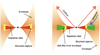 |
Fig. 17 Schematic maps of the CMU model (left; see Sect. 4.1) and the updated model presented in this work (right; see Sects. 4.2.1, 4.2.2, and 4.2.3). The right panel provides similar information to panel f of Fig. 16, but emphasizes a comparison between the locations of the shocked regions in the updated model and the CMU model. |
5.2 Beyond the observations and models
Observationally, this work focuses on the disk-envelope scale. Gas in the inner envelope shows significant infall motion (Sect. 3.1.4), resulting in a surface density much lower than that of the disk traced by millimeter continuum emission dominated by Keplerian rotation. This likely explains why the millimeter continuum size approximately coincides with the inner boundary of the centrifugal barrier traced by the SO ring. While CO (2–1) and SO lines effectively trace emission near the outflow boundaries, probing the inner envelope regions beneath the surface remains challenging. Observations of lower-J transitions, such as CO (J = 1–0) and N2H+, may better constrain these inner layers (e.g., Flores-Rivera et al. 2021), motivating future studies to focus on such tracers.
As is discussed in Sect. 4.2.3, streamers can exhibit specific angular momenta that differ significantly from the global envelope, with some possibly accreting directly onto the disk inside the centrifugal barrier. Due to limited spatial resolution and sample size, this work primarily focuses on shock-related SO and SO2 emission at and beyond the centrifugal barrier. In Oph IRS 63, the SO moment 2 map reveals a spiral-like, broad-line “S” shape (Fig. B.1), which lacks a clear counterpart in the moment 0 map (Fig. 1). The PV diagram along this S structure (Fig. 3a) shows two velocity components in the southeast segment, consistent with shocks confined to the inner envelope surface (Sect. 3). Given the similarity in clockwise spiraling between this S shape and the streamers, this feature may trace accretion flows funneling material from the inner envelope onto the disk (e.g., Hennebelle et al. 2016; Alves et al. 2019; Lee et al. 2020).
Turning to the modeling aspect, this study does not include the effects of magnetic fields on streamer and envelope dynamics (e.g., Hincelin et al. 2016; Wurster et al. 2019; Machida et al. 2020; Tsukamoto et al. 2023; Lesur et al. 2023), nor does it explore the detailed nature of shock types (Flower & Pineau des Forêts 2015). These factors could influence interpretations, especially given the current lack of B-field tracer data. Additionally, the sources examined here are primarily low- to intermediate-mass protostars. For massive young stellar objects, stronger stellar feedback and clustered environments (e.g., Csengeri et al. 2019; Offner et al. 2023; Liu et al. 2024) may expose infalling material to intense radiation before it reaches the centrifugal barrier, altering its dynamics and chemistry.
Despite these limitations, the good agreement between observations and our descriptive model suggests that the accretion shock framework remains a valid approach for understanding the disk-envelope interface in low- and intermediate-mass protostars. Moving forward, expanding observations to larger and more diverse samples – utilizing a variety of shock tracers and targeting protostars with different masses and inclination angles – will be essential for fully characterizing the physical and chemical processes associated with accretion shocks.
6 Summary
In this work, we have searched for and explained signatures of accretion shocks by examining the spectral line emission of SO and SO2 observed by ALMA toward several nearby protostars at different inclination angles (θview). Streamers are commonly observed in these sources (Oph IRS 63 and DK Cha). SO emission tends to concentrate at the centrifugal barrier of the envelope, forming a ring-like structure (Oph IRS 63 and L1527). Outside the centrifugal barrier, SO emission is widely distributed or associated with streamers interacting with the envelopes. Warm spots or segments of SO2 were detected at the feet of the streamers. We propose a disk-like inner envelope model to explain the shock locations and mechanisms traced by both SO and SO2 emission. Below, we summarize the key conclusions of this work:
In Oph IRS 63 (θview ~ 45°), we found an SO2 ring associated with the SO ring surrounding the inner protoplanetary disk. The sulfur-oxide (SO and SO2) ring traces the centrifugal barrier of the infalling envelope at a radius of ~80 au. Outside the sulfur-oxide ring, the velocity distribution of the weak and extended SO emission can be explained by a rotating-and-infalling inner envelope. Four spiral-like streamers are visible in the SO emission (denoted as S1 to S4). A warm spot of SO2 (with Tex ≳ 50 K) is found at the foot of S3, and we suggest that S3 is an off-midplane streamer that violently hits the centrifugal barrier.
In DK Cha (θview ~ 20°), a long segment of ~300 au with broad-line (FWHM of ~ 4 km s–1) emission of SO and SO2 is observed. Two streamers are falling onto the segment, and we speculate that the interaction between the segment and the inner envelope is responsible for the enhancement of SO/SO2. The segment and another streamer feed material into the central disk. A warm spot (~70 K) and a possible hot spot (≳100 K) of SO2 are found at the feet of the streamers. The streamers are also visible in CO emission, located along the outer edges of the SO emission.
In L1527 (θview of ~90°), the SO emission is consistent with prior observations (Sakai et al. 2014, 2017), showing the shape of parallel slabs. This supports the idea that SO emission occurs in ring-like patterns at the surface of a disk or disk-like structure. An “X” shape is seen in the SO PV map; we interpret this as two rings. The velocities of the two rings can be explained by Keplerian motion around a central mass of ~0.5 M⊙. The outer ring corresponds to the centrifugal barrier, as has been noted in the literature. The inner ring may trace the SO snow line. We also detect SO strips along the outer edges of the CO outflow boundaries, which can be reasonably modeled by free-fall trajectories, indicating likely interaction between the outflows and the large-scale envelope surfaces. We propose that there may be an infalling layer warping the outflow cavity, which endures mild shocks.
The model proposed in this work suggests the presence of a disk-like inner envelope outside the centrifugal barrier, formed by the compression of constant-J streams that partly acquire their angular momentum from outflows. While the centrifugal barrier follows Keplerian motion, the disk-like inner envelope exhibits both rotation and infall. Shocks at its surface contribute to the weak, extended SO emission observed beyond the centrifugal barrier. Streamers interacting with this inner envelope deviate from free-fall trajectories, enhancing SO and SO2 emission in their inner regions. Midplane streamers experience continuous shocks, forming warm segments, whereas off-midplane streamers tend to create warm or hot spots due to more violent collisions. The model is consistent with various pieces of observational evidence presented in this work (e.g., sulfur ring, SO streamers, warm spots and segments, envelope motion, infalling layers around outflows).
Overall, SO and SO2 are excellent tracers of accretion shocks around disks. The shock-related chemistry at the surfaces of the disk, the centrifugal barrier ring, and the disk-like inner envelope warrants special attention when studying the chemical and physical properties of protoplanetary disks.
Acknowledgement
X.L. acknowledges the support of the Strategic Priority Research Program of the Chinese Academy of Sciences under Grant No. XDB0800303, and the National Key R&D Program of China under Grant No. 2022YFA1603100. This paper makes use of the following ALMA data: ADS/JAO.ALMA#2022.1.01411.S, #2023.1.00592.S, #2013.1.00708.S, #2019.A.00034.S. ALMA is a partnership of ESO (representing its member states), NSF (USA) and NINS (Japan), together with NRC (Canada), NSTC and ASIAA (Taiwan), and KASI (Republic of Korea), in cooperation with the Republic of Chile. The Joint ALMA Observatory is operated by ESO, AUI/NRAO and NAOJ. We thank the language editor and Dr. Hongli Liu for their valuable grammatical corrections to the manuscript. We thank the anonymous referee for the constructive comments, which helped strengthen this work.
Appendix A Fitting an elliptical ring
We modeled the ring-like emission as an elliptical Gaussian ring characterized by the intensity profile
![Mathematical equation: $I\left( {x,y} \right) = H\exp \left[ { - {1 \over 2}{{\left( {{{r\left( {x,y} \right) - 1} \over \sigma }} \right)}^2}} \right] + C,$](/articles/aa/full_html/2025/09/aa54186-25/aa54186-25-eq49.png) (A.1)
(A.1)
where C is the average background intensity, H is the peak intensity of the ring, and σ represents the ring width normalized by the semimajor axis. The normalized elliptical radius r(x, y) is defined as
 (A.2)
(A.2)
where a and b are the semimajor and semiminor axes of the ellipse, respectively. The rotated coordinates (x′, y′) are obtained by rotating the pixel coordinates (x, y) about the ring center (x0, y0) by an azimuth angle ϕview:
 (A.3)
(A.3)
The parameter set p = (x0, y0, a, b, ϕview, σ, H, C) was determined by fitting the model to the observed 2D emission map using a non-linear least squares optimization method. Initial guesses were based on visual inspection of the data. Fitting was performed using the curve_fit routine from the scipy Python package, and uncertainties on the fitted parameters were estimated from the covariance matrix, with errors reported as one standard deviation (1σ).
Applying this procedure to the moment 0 map of the SO emission in Oph IRS 63 yields the following best-fit parameters: semimajor axis a = 0.50 ± 0.01 arcsec, semiminor axis b = 0.38 ± 0.01 arcsec, azimuth angle ϕview = 52.93° ± 1.14°, normalized ring width σ = 0.52 ± 0.01, peak intensity Η = 50 ± 0.5 mJy beam–1 km s–1, and background intensity C = 20 ± 0.5 mly beam–1 km s–1. The fitted model (Figure A.1) successfully reproduces the elliptical morphology of the ring emission, enabling its geometric and intensity structure to be quantitatively characterized. The inclination angle is estimated as θview = arccos(b/a) ≈ 40.5° ± 1°. We note, however, that the presence of streamers and deviations from a perfectly elliptical ring may introduce systematic uncertainties not captured in the formal error estimates. The interaction between the spiral-like features – particularly S4 – and the SO ring becomes more evident in the residual map after subtracting the fitted ring component (bottom panel of Fig. A.1).
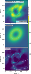 |
Fig. A.1 Upper: Zoomed-in image of the SO ring-like structure of Oph IRS 63. Middle: Best-fit elliptical ring, as described in Sect. A. Lower: Residuals of the SO emission after subtracting the fitted elliptical ring. The dashed cyan line marks the fitted ridge of the elliptical ring. The white lines indicate the four spiral-like structures (see Fig. 1). Note that the field of view in these panels is smaller than in Fig. 1. |
Appendix B Extra images
Images of observations referenced in this work but not included in the main figures will be presented here (Figs. B.1, B.2, and B.3).
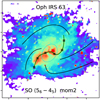 |
Fig. B.1 Moment 2 map of SO (56−45) toward Oph IRS 63, similar to panel (b) of Fig. 2. The green line along the black boxes marks the S-shaped feature observed in the moment 2 map. The black boxes indicate an angular separation of 0.5″, starting from the most bottom left one. |
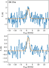 |
Fig. B.2 Upper: Spectrum of SO2 161,15 – 152,14 at position P2 of DK Cha (Fig. 8d), supporting that P1 is a warm (and even hot) spot (Fig. 10). The orange line shows the Gaussian fit. Lower: Same as the upper panel, but for the spectrum smoothed by convolving with a 3-point Flanning window. |
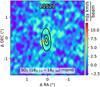 |
Fig. B.3 Moment 0 map of SO2 (163,13 – 162,14) of L1527. The black contours show the ALMA continuum at 1.3 mm same as the white contours in panels a–b of Fig. 13. |
Appendix C Projection of parabolic trajectories
The parallel projection of a parabolic curve in 3D space onto a 2D plane still results in a parabolic curve. In the simplest case (θ0 = θview = ϕ0 = ϕview = 0°; see Fig. C.1), the standard parabolic trajectory of a free-fall stream can be expressed as
 (C.1)
(C.1)
with z = 0, y < –RC in the clockwise case, and y > RC in the counterclockwise case. The free-fall velocity at RC along the parabolic curve is
 (C.2)
(C.2)
At any given point on the standard parabolic trajectory, the projected velocities along the x and y directions are given by
 (C.3)
(C.3)
and
 (C.4)
(C.4)
respectively, with  , and υz = 0.
Denote ℳj,k as the value at the jth row and kth column of a matrix ℳ. Here, we define three matrices ℛi for i = 1, 2, 3. For i = 2, the matrix is given by
 (C.5)
(C.5)
That is,  for k ≠ i, and
  . Similarly, R1 and R3 can be constructed. Denote 𝒜 = (x, y, z) as the points along the parabolic trajectory defined above. Let
 (C.6)
(C.6)
The transformation matrix ℛ can generate the projection of any parabolic trajectory in 3D space through
 (C.7)
(C.7)
Similarly, the projection of the velocity along a parabolic trajectory, denoted as 𝒱 = (υx, υy, υz), can be expressed as
 (C.8)
(C.8)
The observable parameters are the projected components x, y, and υz.
For fixed values of θview and ϕview, the free parameters of the trajectory (𝒜view) are θ0, ϕ0, and RC. The values of θview and ϕview can typically be determined from the morphology of the disk. Note that these values constrain the trajectory to intersect the midplane at a radius of RC. To obtain a parabolic curve without any constraints imposed by the morphology of the disk, the values of θview and ϕview may vary. Only four free parameters are needed to describe all parabolic curves with a fixed focus in 3D space: two parameters to define the plane of the curve, one to specify the axis of the parabola within the plane, and one to determine the focal length. By adopting different values for (θ0, ϕ0,RC, θview), we can generate all such parabolic curves. Fortunately, there are relatively simple methods of determining ϕview, such as measuring the large-scale velocity gradient or the direction of the outflows.
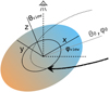 |
Fig. C.1 Schematic illustration of a free-fall stream with a parabolic trajectory (the black line with an arrow), initially originating from (θ0, ϕ0) relative to the disk plane. The black ellipse marks the centrifugal barrier at a radius of RC in the disk plane. The dashed curve represents the extended path of the parabolic trajectory, but the stream does not continue along the dashed curve as it is halted by the centrifugal barrier. Note that we adopt the right-handed coordinate system (x, y, z), and in the case shown here, θview, ϕview, and ϕ0 all have negative values. |
Appendix D Details of equations
For the CMU model (Ulrich 1976; Cassen & Moosman 1981, see also Sect. 4.1), to calculate the density ρ (Eq. 13) at a given point (r, θ), the initial inclination angle of the streamline, θ0, should first be calculated from Eq. 9. This is a cubic equation in one variable. To solve Eq. 9, ChatGPT (OpenAI 2024) provides the solution
 (D.1)
(D.1)
Here, μ = cos(θ), μ0 = cos(θ0),  ,
,  , and D = 4 p3 + 27q2.
For the constant-J model (Sect. 4.2.1), along a trajectory with θ0 ≠ 0°, the azimuthal angle (ϕ) can be expressed as a function of r as
 (D.2)
(D.2)
For any parabolic trajectory, when viewed from the pole, the increment of the azimuthal angle of the trajectory (Δ(ϕ) = |ϕ0 – ϕ|) will always be ≤ 90°. However, when the line of sight is offset from the pole (even with a small θview), the increment of the projected azimuthal angle (Δ(ϕproj)) in some cases can be ~ 180° for a streamline with a small θ0. Therefore, in principle, Δ(ϕ) can have an arbitrary value. Fortunately, if we constrain the trajectory to the midplane (θ0 = 90°), we obtain the following constraint on Δ(ϕproj):
 (D.3)
(D.3)
This can help us to quickly check whether a curved structure can be explained by a free-fall stream that flows in the midplane of the disk (Sect. 3.1.1).
In panel (b) of Fig. 3, the PV curve of a rotating ring is given by the following equations. The arc length of an ellipse is
 (D.4)
(D.4)
Here, k = sin(θview), a is the semimajor axis length, E is the incomplete elliptic integral of the second kind, and ϕ is the azimuthal angle starting from one of the endpoints of the major axis. The projected velocity is expressed as
 (D.5)
(D.5)
Here, Vrot is the rotational speed, and Vsys is the systemic velocity of the ring.
Appendix E Calculation of column density
The column density of a species in the upper-level state (Nu) of a transition is (Mangum & Shirley 2015)
 (E.1)
(E.1)
in the optically thin limit. Here, k is the Boltzmann constant, Tr is the brightness temperature, gu is the upper-level degeneracy, and Debye2 can be expressed in cgs unit as 10–36 cm5g1 s–2. If Tr is not small in comparison to the excitation temperature (Tex), a correction factor (fτ) should be applied,
 (E.2)
(E.2)
with
 (E.3)
(E.3)
Here,  is the peak value of the spectrum in brightness temperature. The total column density of the species can be calculated through
 (E.4)
(E.4)
Here, Q(Tex) is the partition function, which can be interpolated from the tabulated values available online (e.g., through CDMS; Müller et al. 2001), and Eu is the upper-level energy. Eq. E.4 yields (Goldsmith & Langer 1999)
 (E.5)
(E.5)
If multiple transitions are available, the data in the (Eu, ln  ) space represent the rotational diagram. Linear fitting of the data yields the values of N and Tex.
Appendix F Emission along outflow boundaries
The outflow boundaries are manually drawn on the moment 0 map of CO (2–1) of L1527 (Fig. 14). To obatin smoothed boundary lines, cubic interpolation is then applied to the manually selected points along the boundaries (see the resultant black lines in Fig. 14).
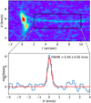 |
Fig. F.1 Upper: PV map of SO emission along the SW direction (same as Fig. 14(c)). Lower: Averaged spectrum (velocity centers of spectra at different r have been corrected for better alignment; see Appendix F for details) of the region enclosed by the black rectangle in the upper panel. The red line shows the Gaussian fit, and the fitted linewidth (FWHM) is labeled. |
F.1 Narrow-line characteristics
The upper panel of Fig. F.1 is identical to Fig. 14, showing the SO emission along the SW boundary of L1527 in the PV map. We denote V0(r) as the fitted free-fall stream velocity in PV space. For each radius r within the main body of the SW region, enclosed by the black rectangle in the upper panel of Fig. F.1, the spectrum along velocity V is resampled by subtracting V0(r) from the velocity axis. This resampled spectrum is denoted as Sr. The spectrum Sr is very narrow in line width (FWHM ~ 0.44 km s–1), confirming the narrow-line feature of the SO strip and the good match with the modeled velocity distribution (dotted white line in Fig. F.1). The stacked spectrum along the SW direction is obtained by combining all Sr over the radius r. The lower panel of Fig. F.1 displays the stacked spectrum and its Gaussian fit, yielding a line width (FWHM) of 0.44 ± 0.05 km s–1. The SO emission along the SE–NW direction (Fig. 14) is also clearly visible in the PV map (Fig. F.2), showing similarly narrow line widths.
F.2 Emission along transverse direction
A line on a 2-D map, such as the outflow boundary, is denoted by a series of points (xi, yi). The transverse direction at the ith point along this line is computed as
 (F.1)
(F.1)
where n = 1 or 3 is chosen to ensure that the transverse arrows point inward toward a specific direction, such as the outflow cavity (Fig. 14).
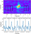 |
Fig. F.2 Upper: PV map of SO emission along the SE and NW directions (same as Fig. 14(d)). Lower: Stacked spectra averaged over different intervals of r, as indicated by the black rectangles in the upper panel. The corresponding intervals are also labeled on the individual spectra. Since the intervals are short, no velocity correction is applied here, unlike in Fig. F.1. |
For the outflow boundary lines of L1527, we first calculated the transverse direction using the method described above. Emission profiles were then extracted along these transverse directions from the moment 0 maps. For both SO and CO, the resulting profiles – averaged over all transverse cuts – exhibit clearly spatially separated Gaussian components. We denote the mean transverse offset of each Gaussian component as μ, with its associated uncertainty represented by σμ. To quantify the significance of the spatial separation between the CO and SO emission, we computed the t-statistic as
 (F.2)
(F.2)
Table F.1 lists the measured transverse separations between the SO and CO emission for the four outflow boundaries in L1527, as illustrated in Fig. 15.
References
- Adams, F. C., Lada, C. J., & Shu, F. H. 1987, ApJ ,312, 788 [NASA ADS] [CrossRef] [Google Scholar]
- Aikawa, Y., Umebayashi, T., Nakano, T., & Miyama, S. M. 1999, ApJ, 519, 705 [Google Scholar]
- ALMA Partnership, Brogan, C. L., Pérez, L. M., et al. 2015, ApJ, 808, L3 [Google Scholar]
- Alves, F. O., Caselli, P., Girart, J. M., et al. 2019, Science, 366, 90 [NASA ADS] [CrossRef] [Google Scholar]
- Artur de la Villarmois, E., Jørgensen, J. K., Kristensen, L. E., et al. 2019, A&A, 626, A71 [NASA ADS] [CrossRef] [EDP Sciences] [Google Scholar]
- Artur de la Villarmois, E., Guzmán, V. V., Jørgensen, J. K., et al. 2022, A&A, 667, A20 [NASA ADS] [CrossRef] [EDP Sciences] [Google Scholar]
- Bachiller, R., & Pérez Gutiérrez, M. 1997, ApJ ,487, L93 [Google Scholar]
- Bacon, R., Accardo, M., Adjali, L., et al. 2010, SPIE Conf. Ser., 7735, 773508 [Google Scholar]
- Bae, J., Teague, R., Andrews, S. M., et al. 2022, ApJ, 934, L20 [NASA ADS] [CrossRef] [Google Scholar]
- Bally, J. 2016, ARA&A ,54, 491 [Google Scholar]
- Banzatti, A., Pascucci, I., Edwards, S., et al. 2019, ApJ, 870, 76 [Google Scholar]
- Bjerkeli, P., van der Wiel, M. H. D., Harsono, D., Ramsey, J. P., & Jørgensen, J. K. 2016, Nature, 540, 406 [Google Scholar]
- Bockelée-Morvan, D., Lis, D. C., Wink, J. E., et al. 2000, A&A, 353, 1101 [Google Scholar]
- Bockelée-Morvan, D., Crovisier, J., Mumma, M. J., & Weaver, H. A. 2004, in Comets II, eds. M. C. Festou, H. U. Keller, & H. A. Weaver (Tucson: University of Arizona Space Science Series), 391 [Google Scholar]
- Booth, A. S., Ilee, J. D., Walsh, C., et al. 2023, A&A, 669, A53 [Google Scholar]
- Booth, A. S., Temmink, M., van Dishoeck, E. F., et al. 2024, AJ, 167, 165 [NASA ADS] [CrossRef] [Google Scholar]
- Brinch, C., & Jørgensen, J. K. 2013, A&A ,559, A82 [NASA ADS] [CrossRef] [EDP Sciences] [Google Scholar]
- Brinch, C., Crapsi, A., Hogerheijde, M. R., & Jørgensen, J. K. 2007, A&A, 461, 1037 [NASA ADS] [CrossRef] [EDP Sciences] [Google Scholar]
- Busch, L. A., Belloche, A., Cabrit, S., Hennebelle, P., & Commerçon, B. 2020, A&A, 633, A126 [NASA ADS] [CrossRef] [EDP Sciences] [Google Scholar]
- Cassen, P., & Moosman, A. 1981, Icarus ,48, 353 [CrossRef] [Google Scholar]
- Chiang, E. I., & Goldreich, P. 1997, ApJ ,490, 368 [Google Scholar]
- Csengeri, T., Belloche, A., Bontemps, S., et al. 2019, A&A, 632, A57 [NASA ADS] [CrossRef] [EDP Sciences] [Google Scholar]
- Draine, B. T., Roberge, W. G., & Dalgarno, A. 1983, ApJ ,264, 485 [CrossRef] [Google Scholar]
- Drozdovskaya, M. N., Walsh, C., Visser, R., Harsono, D., & van Dishoeck, E. F. 2014, MNRAS, 445, 913 [NASA ADS] [CrossRef] [Google Scholar]
- Drozdovskaya, M. N., van Dishoeck, E. F., Rubin, M., Jørgensen, J. K., & Altwegg, K. 2019, MNRAS, 490, 50 [Google Scholar]
- Dutrey, A., Chapillon, E., Guilloteau, S., et al. 2024, A&A, 689, L7 [NASA ADS] [CrossRef] [EDP Sciences] [Google Scholar]
- Eistrup, C., & Walsh, C. 2019, A&A ,621, A75 [NASA ADS] [CrossRef] [EDP Sciences] [Google Scholar]
- Endres, C. P., Schlemmer, S., Schilke, P., Stutzki, J., & Müller, H. S. P. 2016, J. Mol. Spectr., 327, 95 [NASA ADS] [CrossRef] [Google Scholar]
- Fedele, D., van den Ancker, M. E., Henning, T., Jayawardhana, R., & Oliveira, J. M. 2010, A&A, 510, A72 [NASA ADS] [CrossRef] [EDP Sciences] [Google Scholar]
- Feng, S., Codella, C., Ceccarelli, C., et al. 2020, ApJ, 896, 37 [NASA ADS] [CrossRef] [Google Scholar]
- Flores, C., Ohashi, N., Tobin, J. J., et al. 2023, ApJ, 958, 98 [NASA ADS] [CrossRef] [Google Scholar]
- Flores-Rivera, L., Terebey, S., Willacy, K., et al. 2021, ApJ, 908, 108 [NASA ADS] [CrossRef] [Google Scholar]
- Flower, D. R., & Pineau des Forêts, G. 2015, A&A, 578, A63 [NASA ADS] [CrossRef] [EDP Sciences] [Google Scholar]
- Francis, L., Johnstone, D., Herczeg, G., Hunter, T. R., & Harsono, D. 2020, AJ, 160, 270 [NASA ADS] [CrossRef] [Google Scholar]
- Freudling, W., Romaniello, M., Bramich, D. M., et al. 2013, A&A, 559, A96 [NASA ADS] [CrossRef] [EDP Sciences] [Google Scholar]
- Garcia Lopez, R., Nisini, B., Antoniucci, S., et al. 2011, A&A, 534, A99 [NASA ADS] [CrossRef] [EDP Sciences] [Google Scholar]
- Garufi, A., Podio, L., Codella, C., et al. 2022, A&A, 658, A104 [CrossRef] [EDP Sciences] [Google Scholar]
- Gerin, M., Pety, J., Fuente, A., et al. 2015, A&A, 577, L2 [NASA ADS] [CrossRef] [EDP Sciences] [Google Scholar]
- Goldsmith, P. F., & Langer, W. D. 1999, ApJ ,517, 209 [Google Scholar]
- Goodman, A. A., Barranco, J. A., Wilner, D. J., & Heyer, M. H. 1998, ApJ, 504, 223 [Google Scholar]
- Harada, N., Tokuda, K., Yamasaki, H., et al. 2023, ApJ, 945, 63 [NASA ADS] [CrossRef] [Google Scholar]
- Harris, R. J., Cox, E. G., Looney, L. W., et al. 2018, ApJ, 861, 91 [Google Scholar]
- Harsono, D., van der Wiel, M. H. D., Bjerkeli, P., et al. 2021, A&A, 646, A72 [NASA ADS] [CrossRef] [EDP Sciences] [Google Scholar]
- Harsono, D., Bjerkeli, P., Ramsey, J. P., et al. 2023, ApJ, 951, L32 [NASA ADS] [CrossRef] [Google Scholar]
- Hennebelle, P., Lesur, G., & Fromang, S. 2016, A&A ,590, A22 [NASA ADS] [CrossRef] [EDP Sciences] [Google Scholar]
- Hennebelle, P., Commerçon, B., Lee, Y.-N., & Charnoz, S. 2020, A&A, 635, A67 [NASA ADS] [CrossRef] [EDP Sciences] [Google Scholar]
- Hincelin, U., Commerçon, B., Wakelam, V., et al. 2016, ApJ, 822, 12 [NASA ADS] [CrossRef] [Google Scholar]
- Hsu, S.-Y., Liu, S.-Y., Johnstone, D., et al. 2023, ApJ, 956, 120 [Google Scholar]
- Hull, C. L. H., & Zhang, Q. 2019, Front. Astron. Space Sci. ,6, 3 [Google Scholar]
- Keyte, L., Kama, M., Booth, A. S., et al. 2023, Nat. Astron., 7, 684 [NASA ADS] [CrossRef] [Google Scholar]
- Kristensen, L. E., Godard, B., Guillard, P., Gusdorf, A., & Pineau des Forêts, G. 2023, A&A, 675, A86 [NASA ADS] [CrossRef] [EDP Sciences] [Google Scholar]
- Kristensen, L. E., van Dishoeck, E. F., Bergin, E. A., et al. 2012, A&A, 542, A8 [NASA ADS] [CrossRef] [EDP Sciences] [Google Scholar]
- Larson, R. B. 1969, MNRAS ,145, 271 [Google Scholar]
- Lee, C.-F., Ho, P. T. P., Hirano, N., et al. 2007, ApJ, 659, 499 [NASA ADS] [CrossRef] [Google Scholar]
- Lee, C.-F., Li, Z.-Y., & Turner, N. J. 2020, Nat. Astron. ,4, 142 [CrossRef] [Google Scholar]
- Lee, C.-F., Tabone, B., Cabrit, S., et al. 2021, ApJ, 907, L41 [NASA ADS] [CrossRef] [Google Scholar]
- Lesur, G., Flock, M., Ercolano, B., et al. 2023, ASP Conf. Ser., 534, 465 [NASA ADS] [Google Scholar]
- Liang, L., Johnstone, D., Cabrit, S., & Kristensen, L. E. 2020, ApJ, 900, 15 [NASA ADS] [CrossRef] [Google Scholar]
- Liu, X. 2025, arXiv e-prints [arXiv:2502.20458] [Google Scholar]
- Liu, X. C., Wu, Y., Zhang, C., et al. 2021, ApJ, 912, 148 [NASA ADS] [CrossRef] [Google Scholar]
- Liu, X., Liu, T., Shen, Z., et al. 2022, ApJS, 263, 13 [NASA ADS] [CrossRef] [Google Scholar]
- Liu, X., Liu, T., Zhu, L., et al. 2024, Res. Astron. Astrophys., 24, 025009 [CrossRef] [Google Scholar]
- Liu, X., Liu, T., Li, P.-S., et al. 2025, arXiv e-prints [arXiv:2502.10897] [Google Scholar]
- Machida, M. N., Hirano, S., & Kitta, H. 2020, MNRAS ,491, 2180 [Google Scholar]
- Manara, C. F., Morbidelli, A., & Guillot, T. 2018, A&A ,618, L3 [NASA ADS] [CrossRef] [EDP Sciences] [Google Scholar]
- Mangum, J. G., & Shirley, Y. L. 2015, PASP ,127, 266 [Google Scholar]
- Massardi, M., Stoehr, F., Bendo, G. J., et al. 2021, PASP, 133, 085001 [NASA ADS] [CrossRef] [Google Scholar]
- Mauxion, J., Lesur, G., & Maret, S. 2024, A&A ,686, A253 [NASA ADS] [CrossRef] [EDP Sciences] [Google Scholar]
- McElroy, D., Walsh, C., Markwick, A. J., et al. 2013, A&A, 550, A36 [NASA ADS] [CrossRef] [EDP Sciences] [Google Scholar]
- McMullin, J. P., Waters, B., Schiebel, D., Young, W., & Golap, K. 2007, ASP Conf. Ser., 376, 127 [Google Scholar]
- Miura, H., Yamamoto, T., Nomura, H., et al. 2017, ApJ, 839, 47 [NASA ADS] [CrossRef] [Google Scholar]
- Mousis, O., Ronnet, T., Brugger, B., et al. 2016, ApJ, 823, L41 [Google Scholar]
- Müller, H. S. P., & Brünken, S. 2005, J. Mol. Spectr., 232, 213 [CrossRef] [Google Scholar]
- Müller, H. S. P., Thorwirth, S., Roth, D. A., & Winnewisser, G. 2001, A&A, 370, L49 [Google Scholar]
- Mumma, M. J., & Charnley, S. B. 2011, ARA&A ,49, 471 [NASA ADS] [CrossRef] [Google Scholar]
- Neufeld, D. A., & Hollenbach, D. J. 1994, ApJ ,428, 170 [Google Scholar]
- Nisini, B., Santangelo, G., Giannini, T., et al. 2015, ApJ, 801, 121 [NASA ADS] [CrossRef] [Google Scholar]
- Nony, T., Motte, F., Louvet, F., et al. 2020, A&A, 636, A38 [NASA ADS] [CrossRef] [EDP Sciences] [Google Scholar]
- Offner, S. S. R., Moe, M., Kratter, K. M., et al. 2023, ASP Conf. Ser., 534, 275 [NASA ADS] [Google Scholar]
- Ohashi, N., Tobin, J. J., Jørgensen, J. K., et al. 2023, ApJ, 951, 8 [NASA ADS] [CrossRef] [Google Scholar]
- OpenAI 2024, ChatGPT: A Conversational Language Model https://chat.openai.com/, accessed: 2024-10-08 [Google Scholar]
- Oya, Y., Watanabe, Y., L?pez-Sepulcre, A., et al. 2021, ApJ, 921, 12 [NASA ADS] [CrossRef] [Google Scholar]
- Penteado, E. M., Walsh, C., & Cuppen, H. M. 2017, ApJ ,844, 71 [Google Scholar]
- Pickett, H. M., Poynter, R. L., Cohen, E. A., et al. 1998, J. Quant. Spec. Radiat. Transf., 60, 883 [Google Scholar]
- Pineda, J. E., Segura-Cox, D., Caselli, P., et al. 2020, Nat. Astron., 4, 1158 [NASA ADS] [CrossRef] [Google Scholar]
- Podio, L., Eislöffel, J., Melnikov, S., Hodapp, K. W., & Bacciotti, F. 2011, A&A, 527, A13 [NASA ADS] [CrossRef] [EDP Sciences] [Google Scholar]
- Ridge, N. A., Di Francesco, J., Kirk, H., et al. 2006, AJ, 131, 2921 [Google Scholar]
- Riviere-Marichalar, P., Bayo, A., Kamp, I., et al. 2015, A&A, 575, A19 [NASA ADS] [CrossRef] [EDP Sciences] [Google Scholar]
- Riviere-Marichalar, P., Merin, B., Kamp, I., Eiroa, C., & Montesinos, B. 2016, A&A, 594, A59 [NASA ADS] [CrossRef] [EDP Sciences] [Google Scholar]
- Sai, J., Ohashi, N., Maury, A. J., et al. 2022, ApJ, 925, 12 [NASA ADS] [CrossRef] [Google Scholar]
- Sakai, N., Sakai, T., Hirota, T., et al. 2014, Nature, 507, 78 [Google Scholar]
- Sakai, N., Oya, Y., Higuchi, A. E., et al. 2017, MNRAS, 467, L76 [NASA ADS] [Google Scholar]
- Segura-Cox, D. M., Schmiedeke, A., Pineda, J. E., et al. 2020, Nature, 586, 228 [NASA ADS] [CrossRef] [Google Scholar]
- Shu, F. H. 1977, ApJ ,214, 488 [Google Scholar]
- Speedie, J., Dong, R., Teague, R., et al. 2025, ApJ, 981, L30 [Google Scholar]
- Taquet, V., Furuya, K., Walsh, C., & van Dishoeck, E. F. 2016, MNRAS, 462, S99 [NASA ADS] [CrossRef] [Google Scholar]
- Tobin, J. J., Hartmann, L., Chiang, H.-F., et al. 2012, Nature, 492, 83 [NASA ADS] [CrossRef] [Google Scholar]
- Torres, R. M., Loinard, L., Mioduszewski, A. J., & Rodríguez, L. F. 2007, ApJ, 671, 1813 [NASA ADS] [CrossRef] [Google Scholar]
- Tsukamoto, Y., Maury, A., Commercon, B., et al. 2023, ASP Conf. Ser., 534, 317 [NASA ADS] [Google Scholar]
- Tuan-Anh, P., Nhung, P. T., Hoai, D. T., et al. 2016, MNRAS, 463, 3563 [Google Scholar]
- Tychoniec, L., Manara, C. F., Rosotti, G. P., et al. 2020, A&A, 640, A19 [NASA ADS] [CrossRef] [EDP Sciences] [Google Scholar]
- Ulrich, R. K. 1976, ApJ ,210, 377 [Google Scholar]
- Valdivia-Mena, M. T., Pineda, J. E., Segura-Cox, D. M., et al. 2022, A&A, 667, A12 [NASA ADS] [CrossRef] [EDP Sciences] [Google Scholar]
- Valdivia-Mena, M. T., Pineda, J. E., Segura-Cox, D. M., et al. 2023, A&A, 677, A92 [NASA ADS] [CrossRef] [EDP Sciences] [Google Scholar]
- van Gelder, M. L., Tabone, B., van Dishoeck, E. F., & Godard, B. 2021, A&A, 653, A159 [CrossRef] [EDP Sciences] [Google Scholar]
- van Gelder, M. L., Ressler, M. E., van Dishoeck, E. F., et al. 2024, A&A, 682, A78 [NASA ADS] [CrossRef] [EDP Sciences] [Google Scholar]
- van Kempen, T. A., Hogerheijde, M. R., van Dishoeck, E. F., et al. 2006, A&A, 454, L75 [NASA ADS] [CrossRef] [EDP Sciences] [Google Scholar]
- van’t Hoff, M. L. R., Tobin, J. J., Li, Z.-Y., et al. 2023, ApJ, 951, 10 [CrossRef] [Google Scholar]
- Visser, R., & Dullemond, C. P. 2010, A&A ,519, A28 [NASA ADS] [CrossRef] [EDP Sciences] [Google Scholar]
- Visser, R., van Dishoeck, E. F., Doty, S. D., & Dullemond, C. P. 2009, A&A, 495, 881 [NASA ADS] [CrossRef] [EDP Sciences] [Google Scholar]
- Wakelam, V., Ceccarelli, C., Castets, A., et al. 2005, A&A, 437, 149 [NASA ADS] [CrossRef] [EDP Sciences] [Google Scholar]
- Whittet, D. C. B., Prusti, T., Franco, G. A. P., et al. 1997, A&A, 327, 1194 [NASA ADS] [Google Scholar]
- Wurster, J., Bate, M. R., & Price, D. J. 2019, MNRAS ,489, 1719 [NASA ADS] [CrossRef] [Google Scholar]
- Yildiz, U. A., Kristensen, L. E., van Dishoeck, E. F., et al. 2015, A&A, 576, A109 [NASA ADS] [CrossRef] [EDP Sciences] [Google Scholar]
- Zhang, Z. E., Sakai, N., Ohashi, S., et al. 2024, ApJ, 966, 207 [Google Scholar]
- Zhu, Z., Hartmann, L., & Gammie, C. 2009, ApJ ,694, 1045 [Google Scholar]
- Zucker, C., Speagle, J. S., Schlafly, E. F., et al. 2020, A&A, 633, A51 [NASA ADS] [CrossRef] [EDP Sciences] [Google Scholar]
The deconvolution of 2D Gaussians can be performed using the Python package radio_beam (https://radio-beam.readthedocs.io/en/latest/).
All Tables
All Figures
|
Fig. 1 (a) Three-color image of Oph IRS 63, where red, blue, and green represent emissions from the 1.3 mm continuum, SO (56 – 45) (moment 0), and SO2 (83,5 – 82,6) (moment 0), respectively. The synthesized beam is shown in the lower left corner, (b) Moment 0 map of SO (56 – 45) toward Oph IRS 63. The two dashed white ellipses denote the two dust rings of the protoplanetary disk revealed by Segura-Cox et al. (2020). The solid white ellipse represents the SO ring. Four spiral structures (SI to S4) are shown as white curves, (c) Moment 0 map of SO2 (83,5 – 82,6) toward Oph IRS 63. The white ellipse and curves have the same meanings as in panel b. Note that the images shown here represent only a portion of the field of view of the observation and are centered at RA (J2000) = 16h31m35.65s, Dec (J2000) = –24d01m30.1s. |
| In the text | |
|
Fig. 2 Moment 1 (panel a) and moment 2 (panel b) maps of SO (56 – 45) toward Oph IRS 63. In panel a, the directions of the red and blue outflows (Flores et al. 2023) are indicated by the arrows in the corresponding colors. In panel b, the original moment 2 map has been multiplied by a factor of |
| In the text | |
|
Fig. 3 a: PV map of SO along the S-shaped structure observed in the moment maps shown in Fig. 2 (see Fig. B.1 for the implicit marking of the S-shape). The red line marks the location of the SO ring, b: PV map of SO along the sulfur ring (Fig. 1). The white line represents the modeled PV curve of a rotating ring, calculated using Eqs. (D.4) and (D.5). See Sect. 3.1.1 for the fitting results. |
| In the text | |
|
Fig. 4 Models of the four spiral-like structures in Oph IRS 63 (Figs. 1 and 2) generated by free-fall streamers, with colors representing the line-of-sight velocity. Model parameters are provided in Table 2 (Sect. 3.1). The dotted gray lines indicate the observed spiral-like structures (Fig. 1), and the blue ellipse marks the SO ring with a major-axis diameter of 1″ (130 au). The color map corresponds to that in panel a of Fig. 2. Velocities are scaled down by a factor of 2 (from the free-fall values) to approximate the observed velocity range (Fig. 2), with justification provided in Sect. 3.1.2. |
| In the text | |
|
Fig. 5 Moment 0 maps of Οph IRS 63 for four SO2 transitions (Table 1). In panel b, the warm SO2 emission spot (Sect. 3.1.3) is highlighted with a dashed ellipse, which is also shown in panel c for comparison. The black ellipse and curves denote the SO ring and the spiral structures, respectively (Fig. 1). For the moment 0 map of the strongest SO2 line, see Fig. 1. |
| In the text | |
|
Fig. 6 Upper: SO2 spectra of the warm spot in Oph IRS 63, enclosed by a dashed black ellipse in Fig. 5. Lower: rotational diagram of SO2 in the warm spot. |
| In the text | |
|
Fig. 7 a: PV map of SO in Oph IRS 63 along the major axis of the SO ring marked in Fig. 1. The dashed and dotted black lines represent the fits to the velocity distribution of Vϕ with power-law indices of –1 (the free-fall case with non-zero angular momentum) and –0.5 (the Keplerian case), respectively (see Sect. 4.2.2 for details), b: modeled velocity of an inner disk-like envelope (in a simplified 2D version) with its projection parameters (θview and ϕview) identical to those of Oph IRS 63. The radial (υr) and azimuthal (Vϕ) velocities are given by the formulas in the legend, following Eqs. (25) and (24), which describe the possible motion of disk-like inner envelopes (see Sect. 4.2.2 for details). Note that the model is scale-free, and we have adjusted the velocity range and central velocity for better agreement with the observations (panel a of Fig. 2). |
| In the text | |
|
Fig. 8 Moment maps of SO and SO2 for DK Cha. The transition quantum labels are provided at the bottom of each panel, and the beam is indicated in the lower left corner of the first panel. In panel a, the black contours represent the ALMA continuum emission at levels of [0.01, 0.5, 0.9] times the peak value (0.16 Jy beam–1 ). In the other panels, only the 0.5 times the peak value contour of the ALMA continuum is shown. The white contours in the first panel outline the north-east lobe of the outflow, as traced by [S II] 6731 Å using VLT/MUSE. This outflow has been smoothed to match the resolution of the ALMA data. The white contour levels are [0.3, 0.5, 0.7] times the peak value. Substructures identified in the moment 0 map of SO are labeled in the upper left panel, with three streamers (S1 to S3) marked by black curves. For an illustration of additional substructures, their names, and connections, refer to the schematic image in Fig. 12. As in panel b of Fig. 2, the moment 2 map of SO in this figure has been multiplied by a factor of |
| In the text | |
|
Fig. 9 PV maps along the two dotted lines in panel a of Fig. 8. Panels a and b correspond to the northern and southern lines in Fig. 8, respectively. Several gas components identified in Fig. 8 are visible in the PV maps, and are labeled accordingly. |
| In the text | |
|
Fig. 10 Rotation diagrams of the SO2 emission of the two warm spots (P2 and S3 ⊥ P1) of DK Cha (Fig. 8). The emission is extracted at the positions marked by black crosses in Fig. 8. |
| In the text | |
|
Fig. 11 Moment maps of CO (2-1) for DK Cha. Only data within the velocity interval of 0–5 km s–1 were utilized to calculate the moment maps (Sect. 3.2.1). Velocity channels with intensities exceeding 3σ are included in the moment map calculation. In each panel, data outside the dashed white circle have been masked out. White curves represent the streamers identified from the SO emission (Fig. 8). The black contours denote the ALMA continuum, as shown in panel a of Fig. 8. The two ALMA observations were conducted in 2015 and 2023, respectively (Sect. 2). Position shifts due to proper motion and/or possible phase calibration uncertainties have been corrected by cross-matching their continuum peaks, determined via 2D Gaussian fitting. In panel a, the synthesis beams of the CO and SO data are represented by the black and cyan ellipses at the lower left corner, respectively. |
| In the text | |
|
Fig. 12 Schematic image of DK Cha based on its emission of SO and SO2 (Fig. 8). The major gas components that can be seen from the observed data (Fig. 8) are labeled. The black ellipse marks the disk traced by continuum that cannot be fully resolved. The direction of rotation is unknown, and we suggest a clockwise rotation based on the velocity distributions along the streamers and near the disk traced by SO and CO (2-1) (Figs. 8 and 11; see also Sect. 3.2.5). The green ellipse is the assumed disk-like inner envelope, which has strong interaction with the streamers that fall onto it (S1, S2, and S3). The interaction contributes to the enhancement of SO/SO2 emission on the segment (P1) and spot (P2) at the inner envelope (Sect. 3.2). |
| In the text | |
|
Fig. 13 a–b: moment maps of SO of L1527. The white contours represent the continuum emission, with levels of [0.1, 0.5, 0.9] times the peak value. The black contours represent the integrated intensity of SO2 163,13 – 162,14, with levels of [8, 11] Jy beam–1 km s–1. The moment 0 map SO2 is shown in Fig. B.3. In panel b, the beam is shown in the upper right corner by a gray ellipse, c: PV map of SO along the dotted black line in panel b. The solid white and dashed black lines denote the two linear structures on the PV map. |
| In the text | |
|
Fig. 14 a: moment 0 map of CO (2-1) of L1527. The integration range is 0.8–11.6 km s–1. The beam size is shown as black ellipse at the lower left corner. The black lines mark the boundaries of CO outflows, b: moment 0 map of SO, cleaned using the natural weighting (Sect. 2.1.1). To improve the S/N, we have further smoothed the map to a beam size of 0.7″, as indicated by the black ellipse in the lower left corner. The white arrows mark the outflows. The black lines have the same meaning as in the left panel, and are denoted as SW, SE, NW and NE, accordingly to their locations, c and d: PV maps of SO along the outflow boundaries marked in the lower right corners. The dotted white lines represent the fitting results of the trajectories of free-fall streams in PV space (Sect. 3.3.3). See Figs. El and F.2 for the typical spectra of SO along the outflow boundaries. |
| In the text | |
|
Fig. 15 a: same as Fig. 14 but with gray arrows indicating the transverse directions along the outflow boundaries used for extracting radial profiles. The direction of each arrow denotes the positive offset direction, pointing toward the inner regions of the outflow cavities, b–d: averaged emission profiles along the transverse directions for the NE, NW, SE, and SW boundaries (corresponding to panel a). The SO emission is extracted from the image cleaned with natural weighting (without the additional smoothing applied in panel a). For comparison, the CO emission (orange) is divided by a factor of 30 and plotted alongside the SO emission (blue). Dotted lines show the corresponding fits using a Gaussian plus linear function. |
| In the text | |
|
Fig. 16 a: density distribution of the Ulrich (1976) model of the envelope. The black lines are the streamlines, b: same as the first panel but for the constant-J case (Sect. 4.2.1). c: streamline for θ0 = 0 in the constant-J case. Note that ρ depends only on r in the colored region, d: streamlines altered by disk-like inner envelope. The green area represents the disk-like envelope supported by thermal pressure and confined by shocks at the surface (Sect. 4.2.2). The orange area shows the schematic diagram of a Keplerian disk within the centrifugal barrier at RC, with a flare index of 1.3 (e.g., Chiang & Goldreich 1997). The vertical orange-red bar shows the head-on strong shocks at the centrifugal barrier (redder color means stronger shocks). The horizontal blue bar roughly represents the shocked surface of the envelope due to oblique flows, e: streamlines in the envelope viewed from the pole. The gray and yellow regions represent the outer and inner envelopes, respectively. The solid blue line depicts the free-fall parabolic trajectory in the midplane. The dotted and dashed lines are the pressure-modified trajectories in the midplane and on the surface of the inner envelope, respectively, f: schematic map in edge-on view. The gray, green, and orange regions are the outer envelope, disk-like envelope, and the disk, respectively. The black strips are the near-middle-plane (lower left) and off-midplane (upper right) streamers. The arrows indicate the outflows. The red dots highlight the shocked surfaces of the disk-like envelopes. |
| In the text | |
|
Fig. 17 Schematic maps of the CMU model (left; see Sect. 4.1) and the updated model presented in this work (right; see Sects. 4.2.1, 4.2.2, and 4.2.3). The right panel provides similar information to panel f of Fig. 16, but emphasizes a comparison between the locations of the shocked regions in the updated model and the CMU model. |
| In the text | |
|
Fig. A.1 Upper: Zoomed-in image of the SO ring-like structure of Oph IRS 63. Middle: Best-fit elliptical ring, as described in Sect. A. Lower: Residuals of the SO emission after subtracting the fitted elliptical ring. The dashed cyan line marks the fitted ridge of the elliptical ring. The white lines indicate the four spiral-like structures (see Fig. 1). Note that the field of view in these panels is smaller than in Fig. 1. |
| In the text | |
|
Fig. B.1 Moment 2 map of SO (56−45) toward Oph IRS 63, similar to panel (b) of Fig. 2. The green line along the black boxes marks the S-shaped feature observed in the moment 2 map. The black boxes indicate an angular separation of 0.5″, starting from the most bottom left one. |
| In the text | |
|
Fig. B.2 Upper: Spectrum of SO2 161,15 – 152,14 at position P2 of DK Cha (Fig. 8d), supporting that P1 is a warm (and even hot) spot (Fig. 10). The orange line shows the Gaussian fit. Lower: Same as the upper panel, but for the spectrum smoothed by convolving with a 3-point Flanning window. |
| In the text | |
|
Fig. B.3 Moment 0 map of SO2 (163,13 – 162,14) of L1527. The black contours show the ALMA continuum at 1.3 mm same as the white contours in panels a–b of Fig. 13. |
| In the text | |
|
Fig. C.1 Schematic illustration of a free-fall stream with a parabolic trajectory (the black line with an arrow), initially originating from (θ0, ϕ0) relative to the disk plane. The black ellipse marks the centrifugal barrier at a radius of RC in the disk plane. The dashed curve represents the extended path of the parabolic trajectory, but the stream does not continue along the dashed curve as it is halted by the centrifugal barrier. Note that we adopt the right-handed coordinate system (x, y, z), and in the case shown here, θview, ϕview, and ϕ0 all have negative values. |
| In the text | |
|
Fig. F.1 Upper: PV map of SO emission along the SW direction (same as Fig. 14(c)). Lower: Averaged spectrum (velocity centers of spectra at different r have been corrected for better alignment; see Appendix F for details) of the region enclosed by the black rectangle in the upper panel. The red line shows the Gaussian fit, and the fitted linewidth (FWHM) is labeled. |
| In the text | |
|
Fig. F.2 Upper: PV map of SO emission along the SE and NW directions (same as Fig. 14(d)). Lower: Stacked spectra averaged over different intervals of r, as indicated by the black rectangles in the upper panel. The corresponding intervals are also labeled on the individual spectra. Since the intervals are short, no velocity correction is applied here, unlike in Fig. F.1. |
| In the text | |
Current usage metrics show cumulative count of Article Views (full-text article views including HTML views, PDF and ePub downloads, according to the available data) and Abstracts Views on Vision4Press platform.
Data correspond to usage on the plateform after 2015. The current usage metrics is available 48-96 hours after online publication and is updated daily on week days.
Initial download of the metrics may take a while.