| Issue |
A&A
Volume 701, September 2025
|
|
|---|---|---|
| Article Number | A11 | |
| Number of page(s) | 27 | |
| Section | Stellar structure and evolution | |
| DOI | https://doi.org/10.1051/0004-6361/202554710 | |
| Published online | 02 September 2025 | |
The GROND gamma-ray burst sample
II. Fireball parameters for four gamma-ray burst afterglows⋆
1
Max-Planck Institut für extraterrestrische Physik, Giessenbachstr. 1, 85748 Garching, Germany
2
Department of Physics, University of Bath, Building 3 West, Bath BA2 7AY, UK
⋆⋆⋆ Corresponding authors: This email address is being protected from spambots. You need JavaScript enabled to view it.
, This email address is being protected from spambots. You need JavaScript enabled to view it.
, This email address is being protected from spambots. You need JavaScript enabled to view it.
Received:
23
March
2025
Accepted:
7
July
2025
Abstract
Afterglows of gamma-ray bursts (GRBs) are, in general, well described by the fireball model. Yet, deducing the full set of model parameters from observations without prior assumptions has been possible for only a handful of GRBs. With GROND, a seven-channel simultaneous optical and near-infrared imager at the 2.2 m telescope of the Max-Planck Society at ESO/La Silla, a dedicated GRB afterglow observing program was conducted between 2007 and 2016. Here, we combine GROND observations of four particularly well-sampled GRBs with public Swift/XRT data as well as sub-millimetre and radio data from both, our own and other groups’ programmes, to determine the basic fireball afterglow parameters. We find that all four bursts exploded into a wind environment. We are able to infer the evolution of the magnetic field strength from our data, and we find evidence for its origin through shock amplification of the magnetic field of the circumburst medium.
Key words: techniques: photometric / gamma-ray burst: general / gamma-ray burst: individual: GRB 100418A / gamma-ray burst: individual: GRB 110715A / gamma-ray burst: individual: GRB 121024A / gamma-ray burst: individual: GRB 130418A
Based on data acquired with the Atacama Pathfinder Experiment (APEX) under ESO programme 091.D-0131(A).
Present address: Influur Corporation, 1111 Brickell Ave, Miami, FL 33131, U.S.A.
© The Authors 2025
 Open Access article, published by EDP Sciences, under the terms of the Creative Commons Attribution License (https://creativecommons.org/licenses/by/4.0), which permits unrestricted use, distribution, and reproduction in any medium, provided the original work is properly cited.
This article is published in open access under the Subscribe to Open model.
Open Access funding provided by Max Planck Society.
1. Introduction
In the standard gamma-ray burst (GRB) afterglow model, the dominant process during the afterglow phase is synchrotron emission from shock-accelerated electrons in a collimated relativistic blast wave interacting with the external medium (Paczynski & Rhoads 1993; Mészáros & Rees 1997; Waxman 1997). Under the implicit assumption that the electrons are ‘Fermi’ accelerated at the relativistic shocks to a power law distribution with an index p (p > 2 is usually assumed to keep the energy of the electrons finite), their dynamics can be expressed in terms of four main parameters (in addition to p): (1) the total internal energy, E, in the shocked region as released in the explosion; (2) the density and radial profile of the surrounding medium; (3) the fraction of the shock energy going into electrons, ϵe; (4) the fraction of the energy density in the magnetic field behind the shock, ϵB. Both ϵe and ϵB are typically assumed to be constant throughout a burst. The emission spectrum of the forward shock of such an electron population then consists of three segments above the self-absorption frequency νsa (Sari et al. 1998; Granot & Sari 2002): a low-energy tail where Fν ∼ ν1/3, a high-energy power-law segment with Fν ∼ ν−p/2, and an intermediate segment, the slope of which depends on the relative ordering of the cooling frequency, νc, and the characteristic frequency, νm.
With the advent of Swift’s rapid slewing capabilities (Gehrels et al. 2004), the community has collected a wealth of data to trace the temporally and spectrally changing afterglow emission over a wide range of frequencies, from the radio to the γ-rays. This allows us, in principle, to put constraints on the underlying physical model and its boundary conditions.
In practice, this comes with various complications. (i) Bright and/or nearby events allow us to detect additional features on top of the generic afterglow scenario, making it difficult to extract its basic parameters. (ii) In canonical, mostly fainter afterglows, detections at multiple times at multiple frequencies are challenging and thus rarely cover a sufficient spectral and temporal range to infer all basic parameters without extra assumptions. (iii) A substantial fraction of X-ray afterglows show a plateau phase, which is inconsistent with the standard afterglow model. Whether explained from energy injection, as is commonly assumed, or from other processes, such plateaus require additional parameters. (iv) Finally, even in the perfect case where the observational data are consistent with the generic model, the best-fit parameters may fall in unexpected regions in a preferred model scenario.
Examples for the last case are jet breaks and the external density profile. While the standard GRB afterglow model describes the majority of observations, the identification of clear jet breaks in only about 10%–15% of their light curves has been puzzling since the early times of GRB afterglow investigations (Racusin et al. 2009). Several factors may contribute to this, from the lack of multi-wavelength data (to prove the achromatic behaviour) over insufficiently accurate measurements (to identify small decay slope changes) to diverse internal jet structures (changing the light curve profile around the break) or jet orientations relative to the observer (van Eerten et al. 2010). Similarly, the prevalence of a constant radial density profile around GRBs (Panaitescu & Kumar 2001; Schulze et al. 2011) is at odds with the idea that massive stars with strong winds are the progenitors of long-duration GRBs (Chevalier & Li 2000; van Marle et al. 2006).
The aim of the present study is to help form an unbiased picture of the physics of GRB afterglows by adding cases for which all parameters of the standard model can be deduced without any assumption (apart from a synchrotron origin from a decelerating blast wave). We do not include pre-GROND GRBs in our selection process simply because of the spotty multi-wavelength data, in particular near-infrared (NIR) data. From our sample of GROND-observed GRBs (Greiner et al. 2024), we picked four (100418A, 110715A, 121024A, 130418A) for which our multi-epoch, multi-wavelength (e.g. sub-millimetre/radio) observations cover the full range from radio to X-rays so that we could measure the three break frequencies of the synchrotron spectrum and constrain the dust extinction, the X-ray absorption, and the microphysical parameters (this also included testing their constancy).
The paper is structured as follows: In Section 2 we describe the observational data. Sect. 3 presents the modelling approach, separated into phenomenological analysis and derivation of the physical parameters. In Sect. 4 we discuss the results in the context of previously published results.
2. Observations and data reduction
GROND (Greiner et al. 2008), a simultaneous 7-channel optical/NIR imager covering the wavelength range 0.4–2.4 μm (g′r′i′z′JHKs) and mounted at the 2.2 m MPI/ESO telescope at La Silla (ESO, Chile), was designed and developed to rapidly identify GRB afterglows and measure their redshift via the drop-out technique. GROND has observed all well-localised GRBs visible from Chile between GRB 070521 and GRB 161001A. For further details, the observing strategy and some statistics (see Greiner et al. 2024).
We take the GROND-GRB sample as the parent sample because of the importance for well flux-calibrated and simultaneous optical+NIR afterglow data. While we have well-sampled optical/NIR light curves of 54 GRBs with GROND, only eight of those have radio detections. As we show below, these are crucial for the proper modelling of the afterglow. In addition, we only consider those GROND GRBs that have (i) radio afterglow data in at least two radio frequencies over at least two epochs (this excludes GRBs 141026A; Corsi 2014 and 141109A; Corsi & Bhakta 2014) and (ii) a broadband spectral energy distribution (SED) that can be well described by a single synchrotron emission model (this excludes GRBs 081007; Jin et al. 2013 and 090313; Melandri et al. 2010). Thus, we are left with four GRBs.
Here, we analyse observations of GRBs 100418A, 110715A and 130418A, based on public Swift/XRT data, our own extensive GROND monitoring, and the results of our radio (ATCA) and sub-millimetre (APEX) observing programs. Where appropriate, data from other radio or sub-millimetre observations as published in the literature is incorporated. In the final discussion, the analysis results of similar multi-epoch, multi-frequency data of GRB 121024A (Varela et al. 2016) are included.
GROND data were reduced in the standard manner (Krühler et al. 2008) using pyraf/IRAF (Tody 1993; Yoldaş et al. 2008). The optical imaging data (g′r′i′z′) was calibrated against the Sloan Digital Sky Survey (SDSS)1 (Eisenstein et al. 2011), or Pan-STARRS12 (Chambers et al. 2016), and the NIR data (JHKs) against the 2MASS catalogue (Skrutskie et al. 2006). This results in typical absolute accuracies of ±0.03 mag in g′r′i′z′ and ±0.05 mag in JHKs. Finding charts and optical/NIR calibration of the GROND data for our three GRBs are given in Appendix A. Observational details of all multi-wavelength data and their corresponding analysis are described in Appendix B.
3. Fireball modelling
3.1. Procedural notes
We separated our analysis into two parts. The first comprises a model-independent phenomenological analysis where we determine the temporal and spectral slope(s) of the observed flux (using the convention F ∼ t−αν−β, with α and β as the temporal and spectral slope, respectively), and also discuss particular features such as flares, breaks in the light curve, flattening, or any behaviour different from that expected for a canonical afterglow light curve (Granot & Sari 2002). The second part is a model-dependent analysis where we determine the break frequencies and the microphysical parameters by adopting the Granot & Sari (2002) formulation. Details of both steps are given below.
3.1.1. Model-independent analysis
3.1.1.1. Light curve fitting.
The main functions used here for the light curve fitting (and similarly for the SED, using ν instead of t) are
![Mathematical equation: $$ \begin{aligned} F_{\nu }(t) = {\left\{ \begin{array}{ll} F_0 \times \left( \frac{t}{t_0}\right)^{-\alpha } \\ F_1 \times \left[ \left( \frac{t}{t_{\mathrm{1}}} \right)^{-\alpha _1 \mathrm{sm}}+\left( \frac{t}{t_{\mathrm{1}}} \right)^{-\alpha _2 \mathrm{sm}} \right]^{-1/\mathrm{sm}} + \mathrm{host} \\ F_1 \times \left[ F\prime _{\nu }(t_1)^{-\mathrm{sm}} + F\prime _{\nu }(t_2)^{-\mathrm{sm}} \times \left( \frac{t}{t_0}\right)^{-\alpha _3} \right]^{-1/\mathrm{sm}} + \mathrm{host} \end{array}\right.} \end{aligned} $$](/articles/aa/full_html/2025/09/aa54710-25/aa54710-25-eq1.gif) (1)
(1)
for a simple power-law, a smoothly broken, and double broken power-law, respectively (Beuermann et al. 1999). Here, Fi are the normalisation factors at the time, ti; sm is the smoothness of the break, i; αi are the slopes for each power-law segment; and host refers to the contribution of the host galaxy (if detected in late-time observations). The analysis on the temporal evolution provides information on α and possible features like flares, breaks in the light curve, plateau phases and information on the host galaxy (e.g. optical/NIR magnitudes).
3.1.1.2. SED fitting.
The fitting of the SED was performed using XSPEC v12.7.1 (Arnaud 1996). The SED analysis incorporates two steps: First, an analysis of the optical/NIR and X-ray data was performed, including estimates of the dust (UV/optical) and gas (X-ray) attenuation effects along the line of sight due to both the local environment and the host galaxy. Galactic reddening  was taken from Schlafly & Finkbeiner (2011) and a Milky Way extinction law with RV = 3.08 was adopted (Pei 1992). For the host galaxy, templates based on the Small and Large Magellanic Cloud were used (Pei 1992), and the values for extinction
  were derived from our afterglow SED fits.
The second step after the derivation of  ,
,  and β is the inclusion of sub-millimetre and radio data in order to measure the three break frequencies. The slope β of the GROND and XRT bands was allowed to vary within its previous 3σ uncertainty intervals. The smoothness of each break, depending on the temporal slopes in the optical/NIR and the X-rays, is taken from Granot & Sari (2002). The break frequencies were left free to vary. We fit the SED with three breaks but also allowed for the possibility of fewer breaks if not all were covered by our observational range; therefore, the different fit profiles described in Eq. (1) were tested.
3.1.2. Model-dependent analysis
3.1.2.1. The standard afterglow model.
This analysis is explicitly based on the canonical afterglow model as described analytically in Granot & Sari (2002), where the dominant emission is associated with synchrotron radiation from shock-accelerated electrons. These electrons were assumed to have a power-law energy distribution with slope p and minimum energy γm. The observed synchrotron spectrum is characterised by three main break frequencies (νc, νm, νsa) and a peak flux. The synchrotron injection frequency νm is defined by γm. The cooling frequency νc is defined by the critical value γc, above which electrons radiate their energy on smaller timescales than the explosion timescale. The self-absorption frequency νsa marks the frequency below which the optical depth to synchrotron-self absorption is > 1. In this model, two main cooling regimes were defined by the relative position of the break frequencies: a fast cooling regime where νm > νc and most of the electron were cooling fast, and a slow cooling regime where νm < νc (Granot & Sari 2002).
The number of combinations of α and β is limited when a specific dynamical model and the synchrotron spectrum are given, though these are different for wind (k = 2) and ISM (k = 0) density profiles r−k. This gives rise to a unique set of relations between α and β known as “closure relations” (Rees & Meszaros 1994; Wijers et al. 1997; Sari et al. 1998; Dai & Cheng 2001; Zhang 2004; Racusin et al. 2009; Gao et al. 2013). These relations constrain the cooling regime, the circumburst environment, the jet geometry and the electron energy distribution p. The fit results of the multi-power law segment spectrum to the multi-wavelength data is used to both determine all the break frequencies νsa, νm and νc, and to identify the correct (in most cases unique) closure relation. With this solution, we derive the fireball parameters using the relations of Granot et al. (2005) (their Appendix C) for post-jet break SEDs.
3.1.2.2. Handling of plateau phases.
The frequently observed plateaus in the light curve require an additional model ingredient (e.g. Fan & Piran 2006). One possibility is to assume a non-adiabatic (coasting) phase in the jet dynamics where the contact discontinuity between forward and reverse shock, separating ejecta from circumburst medium, is Rayleigh-Taylor unstable. The corresponding cooling of the forward shock will prevent the turn-on of the magnetic field until an observer time later than the deceleration time, thus leading to a plateau phase (Duffell & MacFadyen 2014). While several scenarios were put forward (see Sect. 4.2.4) the more frequently used explanation is prolonged energy injection (Rees & Mészáros 1998; Sari & Mészáros 2000) with the temporal luminosity evolution described via L(t)=Lo t−q, where q is the injection parameter and Lo the initial luminosity. Phenomenologically, the injection parameter can be easily inferred from the light curve analysis. Besides the many observed X-ray and optical plateau phases, prolonged energy injection phases have also been detected in sub-millimetre and radio data (e.g., Jóhannesson et al. 2006; Moin et al. 2013). A simultaneous detection of the plateau phase at all wavelengths implies a dynamical origin for the change in the temporal evolution of the afterglow emission. Physically, the energy injection mechanism depends on the type of the progenitor and the properties of the central engine, and three main mechanisms have been proposed (Sari & Mészáros 2000; Zhang & Kobayashi 2005):
-
A Poynting flux dominated outflow: a magnetar progenitor acts as a long-lived central engine with a constant luminosity, implying q = 0 (Dai & Lu 1998, 2000).
-
Mass stratification: while all material is ejected promptly, different outflow velocities lead to the stratification of shells, i.e., M(γ)∝γ−s. The subsequent collision of the shells (after the first one has decelerated) cause additional injection of energy during the afterglow evolution (Rees & Mészáros 1998). The slope s is related to the injection parameter q: s = (10 − 7q)/(2 + q) and s = (4 − 3q)/q for ISM or wind case, respectively (Zhang et al. 2006; Pe’er & Wijers 2006). For s > 1, corresponding to q < 1, the dynamics of the outflow is altered such that energy injection occurs.
-
Relativistic reverse shock: If the (usually sub-dominant) reverse shock is strong and relativistic, it could mimic an energy injection phase (Kobayashi 2000; Laskar et al. 2013; van Eerten 2014).
After the energy injection phase, only a decelerating forward shock remains and the standard afterglow emission model applies. However, the end of a plateau phase is connected with a break in the light curve, which needs to be distinguished from a canonical jet break. Using the flux and frequency equations for a radial flow from van Eerten & Wijers (2009) and Leventis et al. (2012), we derive the closure relations for a general density profile with an arbitrary k during the deceleration stage following energy injection as  (valid for νm < ν < νc).
3.1.2.3. Additional emission component.
Inverse Compton scattering of synchrotron photons from the relativistic electrons in the afterglow–in the following, we refer to it as synchrotron self-Compton (SSC)–can change the time evolution of the cooling break of the synchrotron component and thus the optical and X-ray afterglow light curves since SSC is an additional (and even more efficient) cooling process than synchrotron. The effect depends on the Comptonisation parameter Y = γ2τe: If Y > 1, which corresponds to ϵe > ϵB. A large fraction of the low energy synchrotron radiation will be up scattered by SSC. We tested the effect of SSC via the C parameter (which is a combination of break frequencies and peak flux, and C < 1/4 holds; see Eq. 4.9 in Sari & Esin 2001), once all parameters had been determined. If SSC dominates, we used the appropriate equations for the physical parameters as given in Sari & Esin (2001) instead of the canonical Granot & Sari (2002).
3.2. Phenomenological analysis
3.2.1. GRB 100418A
3.2.1.1. Afterglow light curve fitting.
The X-ray temporal evolution for the afterglow of GRB 100418A (Fig. 1) is well described by a double broken power-law with smooth breaks (see Eq. 1). The plateau phase (αEI = −0.21 ± 0.12 up to tb2 = 82 ± 29 ks) after the initial steep decay (with αpre = 4.16 ± 0.08) may be associated with an ongoing energy injection phase (Marshall et al. 2011). The late decay (αpos = 1.61 ± 0.19) can be associated with the normal afterglow decay where the break time is associated with either the end of the ongoing energy injection or a jet break.
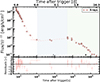 |
Fig. 1. X-ray light curve of GRB 100418A from the XRT repository. The best fit is a smoothly double broken power-law shown in dashed lines. The epochs used are marked by vertical shaded regions: the steep decay phase (white), the plateau phase (blue), and the post-energy injection phase after a jet break (light green). |
The optical/NIR light curve (Fig. 2 and Table B.1) in all 7 bands (g′r′i′z′JHKs) starts with a shallow decay around 104 s, followed by a steeper decay. The best fit describing the observations is a smooth broken power-law with host contribution, with best fit parameters αpre = 0.32 ± 0.04, αpos = 1.41 ± 0.04, tb = 73.6 ± 2.5 ks, sm = 15 ± 11 (χ2/d.o.f = 181/184). The Swift/UVOT observations in the white band (Siegel & Marshall 2010) and the observations in the Rc band (Bikmaev et al. 2010; Hattori & Aoki 2010) show a fast increase in flux between 2000 s and 7000 s, which could be the result of a flare on top of the plateau phase (Marshall et al. 2011) or a refreshed shock. However, since it is not covered by either Swift/XRT or GROND, it is difficult to determine the real cause. After this time, the behaviour is consistent with GROND; the possible flare contribution is not taken into account in our study.
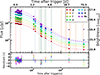 |
Fig. 2. GROND light curve g′r′i′z′JHKs of the afterglow of GRB 100418A. The best fit of the combined optical/NIR and X-ray data is a smooth broken power-law with host contribution shown in dash lines. The epochs used for the spectral analysis are highlighted with the vertical bars. The first two epochs highlighted in light red correspond to the energy injection phase. The last five epochs in orange correspond to the slow cooling regime, the earlier epochs to fast cooling (see Sect. 3.3.1). For the blue epochs joint GROND-XRT SEDs were produced (see Fig. 4 and Sect. 3.2.1). The green and orange epochs correspond to the SED analysis that includes radio data (Sect. 3.3). |
Given that after T+10 ks the XRT and GROND data are both described well by a smooth broken power-law with consistent best-fit parameters, a better constraint on the break time is obtained by a combined fit of both the XRT and GROND data. The main difference between the combined and the individual data sets are the values of the pre-break slopes. We performed three different fits (all of them with the break time linked): the best fitting model is that with only the post-break slopes linked, resulting in fit parameters of  and
and  , tb = 76.4 ± 2.7 ks, sm = 6.9 ± 1.3 and αpos = 1.46 ± 0.04, but the fit with also the pre-break slopes linked is only marginally worse.
Observations with SMA at 340 GHz begin at ∼0.8 days post trigger and are well described by an initial decay with  up to tb ∼ 126 ks, followed by a plateau phase of
  (Fig. 3). Further observations at three epochs with PdBI at 106 GHz and 103 GHz are well described by a single power-law with a slope α ∼ 0.75. In contrast, PdBI observations at 867 GHz are described by an initial slope with α ∼ 2.1 up to tb1 ∼ 8.2 × 10⁵ s followed by a plateau phase with α ∼ 0.23 up to tb2 ∼ 3.1 × 10⁶ s and a final decay phase with α ∼ 1.5 (Fig. 3). The observations with ATCA at 9.0 GHz and 5.5 GHz show a constant flux from 105 s to 106 s. However, it is possible that the first observations are affected by interstellar scintillation effects, and therefore the actual flux might be lower. The VLA data show an increase in the flux with α ∼ −1.0 up to tb ∼ 4 × 10⁶ s and then a decay phase with α ∼ 2.1 (Fig. 3). The scintillation effects on the observations were included as an additional error on the individual observations.
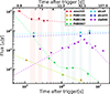 |
Fig. 3. Sub-millimetre and radio light curves of the GRB 100418A afterglow at different frequencies. Dashed lines show the best fit. The eight highlighted vertical regions correspond to the epochs used in the SED analysis. The orange (blue) regions correspond to the fast (slow) cooling regime. The light curves were scaled by an arbitrary factor for clarity. |
3.2.1.2. Afterglow SED fitting.
We used seven epochs with combined XRT and GROND data: two epochs during the plateau phase and five epochs after the break in the light curve (Fig. 4). The best-fit host galaxy magnitudes from the last epoch were subtracted from the optical/NIR data. In our fits, the host galaxy dust extinction and gas absorption were linked between all SED epochs.
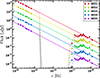 |
Fig. 4. Spectral energy distributions of the afterglow of GRB 100418A using GROND and XRT data at five epochs: SED1 (t = 130.9 ks), SED2 (t = 202.1 ks), SED3 (t = 217.8 ks), SED4 (t = 296.8 ks), and SED5 (t = 476.4 ks). For clarity, the SEDs were scaled arbitrarily (GROND magnitudes are given in Table B.1). The best-fit SED slope is β = 1.11 ± 0.02. |
For the two epochs during the plateau phase (red regions in Fig. 2), the SED slopes were initially left free to vary; the fits consistently have the same slope in both cases ( and
and  , respectively). When we tied the SED slopes, the fit returns a spectral index
  and host dust extinction given by a Small Magellanic Cloud (SMC) reddening law (Pei 1992)
  mag. In the case of the X-ray SEDs, the observations during the three analysed epochs are well described by a power-law with β = 0.94±0.12,
  =
=  × 1020 cm−2 and a goodness of the fit of χ2/d.o.f = 7.4/9.
Optical and X-ray segments at later times have the same spectral slopes and can be described by a power-law. The XRT SED epoch between t = 100 ks to t = 300 ks is described by a mean spectral slope  with a goodness of the fit of χ2/d.o.f = 9.0/12 and
  cm−2. The five GROND epochs have a spectral slope
  . All the slopes were linked between the five SEDs. This is completely consistent with the fit with unlinked slopes, and therefore, it is evident that there is no spectral evolution. The combined fit results in a best-fit power-law with slope β = 1.11 ± 0.02. The fact that this is slightly steeper than the separate GROND and Swift/XRT fits is likely due to the inaccuracy of the absolute flux calibrations between optical/NIR and X-ray bands. The host dust extinction is given by a Small Magellanic Cloud (SMC) reddening law (Pei 1992) with a value
  mag. The gas column density is
  cm−2 and the goodness of the fit is χ2/d.o.f = 85/101. These constraints are going to be used as base values for the analysis in the following sections.
3.2.1.3. Broadband SED analysis.
When including the sub-millimetre and radio data a spectrum with three breaks is necessary to describe the observations; the gently curved SED in the 1010–1012 Hz range is too broad to be fit with two breaks (Fig. 5). In total, eight epochs were used (Table 1 and Table B.2); these epochs were selected for the availability of radio data, and are distinct from the GROND-SED epochs shown in Fig. 4. All the epochs were fitted simultaneously, with the only constraints being  and
and  as derived previously. The slope of the GROND and XRT bands was allowed to vary within a 3σ uncertainty interval around their previous best fit. The smoothness of each break depends on the temporal slopes in the optical/NIR and the X-ray (Granot & Sari 2002). Fig. 5 shows the final fit for each SED, the best-fit frequencies are given in Table 1, and their movement with time is shown in Fig. 6. The assignment of the nature of the breaks and the determination of the physical parameters is done in Sect. 3.3.1 based on the Granot & Sari (2002) framework.
Break frequencies for the eight epochs of the GRB 100418A afterglow using a double broken power-law.
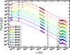 |
Fig. 5. Broadband SED analysis for GRB 100418A using eight epochs analysed using multi-epoch broadband observations. The first three epochs correspond to the fast cooling regime (SED1r – SED3r); the last five epochs (SED4r – SED8r) correspond to the slow cooling regime. The best-fit model for all SEDs is a double broken power-law with smooth breaks. |
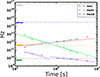 |
Fig. 6. Evolution of the measured break frequencies for the eight optical to radio SEDs for the GRB 100418A afterglow. The solid lines represent the expected theoretical evolution for a wind environment during fast (< 600 ks) and slow (> 600 ks) cooling. The coloured dashed lines represent the best power-law fits to the measured temporal evolution (open data points were left out from the fit). The horizontal dashed lines show the mean frequencies of our data (X-ray, optical, sub-millimetre, radio). |
3.2.2. GRB 110715A
3.2.2.1. Afterglow light curve fitting.
The analysis follows the same methodology as for GRB 100418A: After individual X-ray (final decay with slope αpos = 1.34 ± 0.07; Fig. 7) and GROND (single power law with slope α = 1.51 ± 0.03; Fig. 8) fits, a combined fit results in αpos = 1.48 ± 0.05 for both, optical/NIR and X-ray data (χ2/d.o.f = 192/143). We note that the time before the first GROND epoch was covered by Swift/UVOT and Rc band observations (Kuin & Sonbas 2011; Nelson 2011), and they show a plateau phase similar to that in the X-ray light curve.
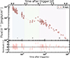 |
Fig. 7. X-ray light curve of the GRB 110715A afterglow described by a smooth double broken power-law shown in dashed lines. The three regions used in the SED analysis are shown as shaded areas, corresponding to the GRB tail, the plateau and the final decay phase, respectively. |
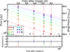 |
Fig. 8. GROND g′r′i′z′JHKs light curve of the GRB 110715A afterglow. The best fit is a single power-law with α = 1.51 ± 0.03, as shown with the dashed lines. The epochs used for the spectral analysis are highlighted with the vertical bars. All four epochs are after the plateau phase. |
Observations with APEX and ALMA at 345 GHz show a decaying flux between the two epochs, with a slope of αsub = 0.87 ± 0.23 (Sánchez-Ramírez et al. 2017). The six ATCA epochs at 44.0 GHz are described by a smoothly broken power-law, with slopes of αpre = –3.61 ± 0.71 and αpos = 0.91 ± 0.12 before and after the break at tb = 325.2 ± 28.2 ks, respectively. The decay slope is consistent with the observations at 345 GHz. A similar behaviour is observed at 18 GHz, but with a late break time of tb2 = 613 ± 102 ks. Finally, at frequencies of 9.0 GHz and 5.5 GHz the flux remains almost constant throughout the observations, with α = 0.09 ± 0.07 and α = 0.08 ± 0.11, respectively. At 5.5 GHz there is a change in the temporal evolution just before the last epoch where there is a steep decrease in flux with slope α ∼ 1.8. The sub-millimetre and radio light curve fits are shown in Fig. 9.
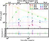 |
Fig. 9. Sub-millimetre and radio light curves of the GRB 110715A afterglow. The best fit for each of the bands is represented by dashed lines. The six highlighted vertical regions correspond to the epochs used in the broadband multi-epoch SED analysis. The light curves were scaled by an arbitrary factor for clarity. |
3.2.2.2. Afterglow SED fitting.
Three X-ray SEDs were analysed before (3.7–12.1 ks), during (22.3–56.4 ks), and after (62.3–849.1 ks) the plateau phase (see Fig. 7). The best-fitting profile is a simple power-law with  cm−2 and slopes βpre = 1.01 ± 0.15, βEI = 0.85 ± 0.09 and βpos = 1.06 ± 0.13. For the analysis of the optical/NIR SEDs, the four slopes are very similar, and a fit with all four epochs linked results in
  mag and β = 0.35 ± 0.12 (χ2/d.o.f = 14/22). A combined analysis of the XRT and optical/NIR observations was performed in order to check if a simple power-law can successfully describe the observations or if the suggested 0.65 slope difference is real. The XRT SEDs were renormalised to match the mid-time X-ray flux at the time of each of the optical SEDs. It turns out that a single power-law is indeed sufficient, leading to best fitting parameters of β = 1.05 ± 0.01,
  ,
,  (see Fig. 10).
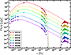 |
Fig. 10. Broadband analysis of the GRB 110715A afterglow. Six epochs are presented with all the breaks measured. |
Break frequencies for the six epochs of GRB 110715A using broadband observations.
3.2.2.3. Broadband SED fitting.
Six epochs of SEDs including the sub-millimetre and radio data were fitted using a double broken power-law with smooth breaks. Table 2 summarises the break locations for all epochs, and Fig. 11 shows their movement with time.
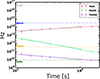 |
Fig. 11. Evolution of the break frequencies of the afterglow of GRB 110715A. The last SED is not included in the fit because the values for the optical/NIR bands were extrapolated. Lines are as in Fig. 6. |
3.2.3. GRB 130418A
3.2.3.1. Afterglow light curve fitting.
While a single power-law fit to the X-ray data would be acceptable (α = 1.47 ± 0.06 with χ2/d.o.f = 28/18), the optical/NIR light curves from GROND (Fig. 13 and Table B.6) and data from the literature (Gorosabel et al. 2013; Quadri et al. 2013; Klotz et al. 2013; Butler et al. 2013) require two breaks (Fig. 12). The best fitting parameters of the combined observations are:  and
and  , a break time tb1 = 18.8 ± 3.5 ks with smoothness sm = 5.4 ± 1.3 followed by a decay with slopes αEI = 1.11 ± 0.14 up to tb2 = 61.7 ± 8.1 ks with smoothness sm1 = 3.3 ± 0.8 and a final decay slope of αpos = 2.40 ± 0.19 (χ2/d.o.f = 242/195). The observations in the sub-millimetre and radio wavelength range show a rising and then fading flux at 340/345 GHz (SMA and APEX).
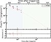 |
Fig. 12. X-ray light curve of the afterglow of GRB 130418A with the early WT data omitted. The highlighted vertical regions corresponds to the two main epochs of the SED analysis. |
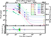 |
Fig. 13. Optical/NIR light curve of the afterglow of GRB 130418A observed with GROND, including data from the literature. The best-fit model is a double broken power-law with smooth breaks, and includes a host detection at r′(AB) = 25.4 ± 0.3 mag. |
3.2.3.2. Afterglow SED fitting.
The X-ray data are best described by a single power-law with slope β = 0.58 ± 0.11 with  cm−2. Three GROND SEDs were used, two before the break in the light curve at tb = 45.4 ks and one after. The combined fit linking the individual slopes and the host
  provide best fitting parameters of
  = 0 and spectral slope β = 1.16 ± 0.07. A combined XRT/GROND SED was not possible given the non-matching coverage.
3.2.3.3. Broadband SED analysis.
For the fits including the radio and sub-millimetre data, the values for the dust and gas attenuation effects  ,
,  ,
,  ,
,  along the line of sight were set to the values obtained in the previous section. Three spectral breaks are required, and the results are shown in Table 3 and in Fig. 14. The evolution of the break frequencies is shown in Fig. 15.
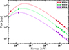 |
Fig. 14. Broadband SEDs of the GRB 130418A afterglow at the three epochs of Table 3. Data are given in Table B.6. |
3.3. Physical parameters of the standard afterglow model
We now proceed with the derivation of the microphysical and dynamical parameters of the GRB afterglow, based on the standard afterglow model and including the effect of inverse Compton scattering as an additional possible way for the ‘Fermi’ accelerated electrons to cool down. For GRB afterglows with a plateau phase, we use the concept of energy injection as a valid interpretation, which affects the pre-break slopes. During the plateau phase, the cooling can be either fast (νc < νm) or slow (νm < νc), with the blast wave moving into a stellar wind-like or an ISM external density profiles. The end of the plateau phase can be associated with the end of an ongoing energy injection phase, a jet break, or both.
We followed two main steps to analyse the afterglow data: (1) Spectral regime: Considering the movement of the break frequencies, we applied the closure relations (Racusin et al. 2009) to determine the external density profile, the spectral regime, and the electron index p of the distribution of the accelerated electrons. We tested these for each possible option of the observing frequency (Table 1) being in any of the synchrotron spectral regimes. (2) Microphysical and dynamical parameters: We compared the fits of the full multi-wavelength data to the standard formalism for a spherical blast wave propagating into an external cold medium during the fast and slow cooling regime (Granot & Sari 2002; Dai & Cheng 2001; Leventis et al. 2012), and we subsequently checked for consistency with the slow and fast cooling transition times. The half-opening angle of the jet was derived using Eq. (4) from Granot et al. (2005). For the efficiency of the conversion of the kinetic energy in the outflow to gamma-rays during the prompt emission, we used  ), where
  is the isotropic energy released in the prompt gamma-ray emission calculated using
  =4πdL2F/(1 + z), with F the fluence in the rest-frame energy range 1 − 104 keV. For the radial profile of the external density, we followed the canonical k = 0 (constant, ISM-like) and k = 2 (wind profile) description. For the k = 2 case, we report the density in terms of A* = A/(5 × 1011g cm−1) (Chevalier & Li 2000).
3.3.1. GRB 100418A
3.3.1.1. Closure relations.
Applying the closure relations to the X-ray/optical/NIR data and based on the measured post-break temporal slope and because no spectral evolution is detected between the observations before and after the break in the X-ray or optical bands (which excludes the passage of a break frequency), three possible scenarios are in agreement with the observations:
-
An afterglow with the plateau phase is associated with an ongoing energy injection into the outflow. The implied injection parameter is q = 0.23 ± 0.05 (from the fit with linked pre-break slopes). This is followed by a normal decay phase associated with a radial outflow with no energy injection. The outflow is evolving into an ISM external medium, and the optical and X-ray data is on the spectral segment between νm and νc.
-
A break in the light curve at the end of the plateau phase is associated with a uniform non-spreading jet. In this case the outflow is propagating into a stellar wind-like medium. The X-ray/optical/NIR observing frequencies are above νc and νm. The cooling regime can be either fast or slow since both have the same temporal and spectral indices.
-
The end of the plateau phase is associated with the end of the prolonged energy injection and a uniform spreading jet. Within a 3σ uncertainty error bars, the external medium is consistent with both ISM or stellar wind-like medium.
Including the temporal evolution of the radio data is then used to determine which of the above three scenarios is preferred. First, the SMA flux is constant or slowly decreasing. Thus the optical and SMA bands have to be in different segments of the synchrotron spectrum. The SMA data would be consistent with an ISM or stellar wind-like external medium in the fast cooling regime for νc < νSMA < νm, but also with a stellar wind-like external density profile in the slow cooling regime with the SMA wavelength between νsa and νm. This is only consistent for a stellar wind-like density profile with νc below the optical data and the end of the plateau phase being associated with both the end of the energy injection and a (non-spreading) jet break. The PdBI data at 106 GHz, 103 GHz and 86.7 GHz are consistent with this model where the fast cooling regime continues until t ∼ 600 ks, and the PdBI wavelengths lie between νsa and νc. The ATCA and VLA radio data then fall in the slow cooling regime, and are consistent with the expected temporal and spectral slope. The favoured scenario is therefore a plateau phase due to energy injection, and the end of the plateau phase is associated with the end of the energy injection together with a uniform non-spreading jet break expanding into a stellar wind-like density profile (above scenario 2). We recall that GROND and XRT data are above νc and νm, and therefore the electron index is p = 2.22 ± 0.04.
3.3.1.2. Afterglow parameters.
The analysis of the SEDs during the early fast cooling regime and the (later) slow cooling regime was done separately as the dependencies of the break frequencies on the parameters are different. All the results are reported in Table 4 and Table 5.
Derived microphysical and dynamical parameters for the GRB 100418A afterglow from the five epochs of slow cooling.
Fast cooling. During the early fast cooling phase (SED1-SED3) inverse Compton scattering is expected to play an important role in the cooling of the electrons. We test the strength of the inverse Compton scattering, but find ϵB ≫1, leaving the model with no physical meaning.
We double-checked the fitting with the set of equations given by Granot et al. (2000), but confirm that no consistent solution is obtained. As mentioned in Granot & Sari (2002), the emission during fast cooling in a wind environment is no longer dominated by the shock front but tends to come from smaller radii, and thus the break frequencies and corresponding flux densities are different by up to a factor of three between Granot et al. (2000) and Granot & Sari (2002). We therefore cannot deduce physical parameters from the 3 first epochs of evolution of the GRB 100418A afterglow.
Slow cooling. The last five epochs of the afterglow observations, i.e. SED4-SED8, are used in this case. The dynamical and microphysical parameters are in complete agreement with the theory. The inverse Compton scattering contribution was tested, because the low value of νc and the large A* are indicative of SSC. However, we find no dominant contribution.
All the values with and without SSC cooling are within the expected values from the theory. The average value for ϵe is about 0.36, and for EK, iso, it is about 2 × 1052 erg. The relation ϵe/ϵB is < 10, which is in agreement with the SSC contribution being negligible during the slow cooling phase, and it is therefore not included in the rest of the discussion. The value of A* (no SSC included) is of order unity, and ϵB is about 0.1, which could require a larger value of B in the shocked region. However, the temporal evolution of B (α = –0.81±0.05), as seen in Fig. 16, is as expected (α = –3/4) of a magnetic field generated by shock compression of the seed magnetic field in the circumburst medium (CBM). Therefore, the difference in the expected values might just be related to the actual magnitude of B0. If B0 is of the order of a few milligauss, the value derived for ϵB is reproduced by theory.
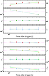 |
Fig. 16. Slow cooling: Evolution of the derived dynamical (top) and microphysical (bottom) parameters of the afterglow of GRB 100418A without SSC emission. The blue dashed lines and shaded regions represent the results from the fit of the observed temporal evolution. The horizontal dashed purple lines show the average value for each parameter. EK, iso is in units of 1052 erg. |
3.3.1.3. Overall picture.
(a) The cooling regime is initially ‘fast’ cooling, with νm > νc up to about 600 ks, and later the transition to slow cooling with νc > νm. (b) The CBM profile corresponds to a stellar wind-like density profile. (c) The break frequency evolution is shown in Fig. 6 and consistent with evolution in wind environment. (d) The light curve plateau is compatible with continuous energy ejection. (e) The observed light curve break is due to both, the ceasing of the energy injection and the jet break of a uniform non-spreading jet with a collimation angle of about 0.22 rad. (f) The energetics is described with a mean EK, iso of about 2 × 1052 erg, and when compared with  , a required efficiency of about 6%. (g) The emission mechanism is synchrotron, and some SSC contribution is possible.
3.3.1.4. Comparison with literature.
Our fitting results are consistent with those of Marshall et al. (2011), but they interpret the light curve break after one day as a consequence of the ceasing energy injection instead of a jet break, deduce a large beaming angle and very high beaming-corrected energy.
Laskar et al. (2015) have analysed Swift/UVOT data and selected optical data published in GCNs. They provide solutions for 100418A for both, ISM and wind profile, and prefer the ISM solution because of the implied lower energy put during the energy injection phase. However, we note that this choice hinges on one single Rc-band data point, which suggests a very rapid optical rise during the first few hours. While our GROND data do not cover this early phase, the flat portion of the GROND light curve as well as the Swift/UVOT data suggest a much more modest flux increase. The parameters of our best-fit model are fully consistent with their wind solution.
3.3.2. GRB 110715A
3.3.2.1. Closure relations.
The analysis of the first segment of the XRT observations (t < 21.4 ks) is in agreement with νm < νXRT < νc with an energy injection component in an ISM or stellar wind-like density profile, or in an ISM density profile without the energy injection component. However, the observations during this time interval might be altered by the contribution from SSC, and therefore the closure relations could be modified, i.e., α is steeper when SSC is dominant. If SSC is included only νc < νXRT is in agreement with the observations for either an ISM or a stellar wind-like density profile. A strong reason to have a SSC contribution is that it could explain the first break in the light curve, otherwise, the plateau phase would require a central engine that can ‘restart’ itself after 104 s. Therefore, the break would just be associated with the end of a dominant inverse Compton phase and the energy injection phase would just continue until the second break.
The plateau phase is in agreement with two scenarios: an energy injection phase where νXRT < νc and q = –0.25 ± 0.10 for an ISM external medium and p = 3.10 ± 0.02, or alternatively νXRT > νc with q = –0.36 ± 0.15 for p = 2.10 ± 0.02 in either a stellar wind-like or an ISM density profile. The second break in the X-ray light curve is associated with the end of the energy injection phase and/or with a jet break. Observations at the optical and X-ray frequencies have the same temporal slope during this last time interval, which is in agreement with both.
Three cases fit the data during this last time interval: first, for νXRT < νc with the break associated only to the end of the energy injection phase in an ISM density profile. Second, where νc < νXRT and the break is associated with both the end of an energy injection phase and a uniform non-spreading jet break in a stellar wind-like density profile. Third, νc < νXRT with the break in the light curve associated uniquely to a non-spreading jet break but with an ongoing energy injection phase.
Including the sub-millimetre and radio data, we first recall that below νm the flux at sub-millimetre and radio wavelengths would evolve with the same slope in an ISM density profile. Since this is not observed, any scenario where the CBM is homogenous can be discarded. The evolution of the frequencies as shown in Fig. 11 (νsa: α = –0.72 ± 0.10; νc: α = 0.56 ± 0.10) supports slow cooling and a stellar wind-like density profile. Therefore, the plateau phase can only be explained by a stellar wind-like density profile when q = –0.36 ± 0.15 and νc < νXRT. As no SED evolution is detected in the XRT or optical/NIR bands, this implies that the observations during the pre- and post- plateau phase must be in the same spectral regime. Therefore, the pre-plateau phase is best explained by an IC contribution in a spectral regime where νc < νXRT. Finally, the post-plateau phase observations can be described by the νc < νXRT regime (and wind-like CBM) and the break associated with a uniform non-spreading jet with or without the end of the energy injection phase.
In this last scenario, however, having a source that provides such long energy injection and without a sign of it at least in the sub-millimetre region is non-standard. Therefore, the only credible scenario is the association of the break in the light curve after the plateau phase with the end of the energy injection phase together with a uniform non-spreading jet in a stellar wind-like density profile for νc < νXRT. A change in the flux evolution due to the non-spreading jet break would then take place compared to the normal evolution. The change is (k–3)/(4–k), i.e., –3/4 for an ISM density profile and –1/2 for a stellar wind-like density profile. We therefore propose the stratification of shells as the favourable scenario for the energy injection phase with a strong contribution from IC during the early epochs.
The radio and sub-millimetre observations have some discrepancies from the theoretical results. The flux from observations at 9.0 GHz and 5.5 GHz have an evolution with temporal slopes α = –0.08 ± 0.11 and α = –0.09 ± 0.07, respectively. In the case of a stellar wind-like density profile with a non-spreading jet break, the expected slope is α = –1/2, which is 3.5σ and 5.3σ away from the observed α at 9.0 GHz and 5.5 GHz, respectively. This could be associated with a strong interstellar scintillation effect, which is stronger at lower radio frequencies. Observations at 18 GHz are expected to have an initial slope of α = -1/2 and then a decreasing flux with α = 1/2. The observations are consistent with this within 2σ uncertainty.
Finally, for observations at 44 GHz and 345 GHz, the flux is expected to decrease with α = 1/2. Observations at 345 GHz, and after the second epoch at 44 GHz show a decrease in flux with an α of about 0.91 ± 0.12, although it is 3.4σ away from the expected value, the difference might just be due to the low statistics in the sample. It is, however, not clear why the first two epochs, at a frequency of 44 GHz does not follow the expected values and are rapidly increasing with a slope of about -2. There is clearly an external effect that must be affecting the observations during these epochs, specially the first observation. If the flux at the first epoch is larger, then the rate of the increase in the flux would be slower, and it could be in agreement with the –0.5 if ν < νsa. This is a possible scenario where νsa just crosses ν at 44 GHz as seen in the following section.
3.3.2.2. Afterglow parameters.
From the analysis so far, we conclude that the best scenario describing the (late) observations is a uniform non-spreading jet expanding into a stellar wind-like density profile. The afterglow evolution went through an energy injection phase before the jet break. The power-law index p of the non-thermal electron population is p = 2.10 ± 0.02. The cooling break is located below the NIR wavelengths, and thus no spectral evolution in the optical/NIR or X-ray bands is observed.
The measured break frequencies are used to derive the dynamical and microphysical parameters. The effect of energy injection is not taken into account, as it finishes before the start of the six analysed epochs. The results for all the parameters are reported in Table 6 and in Fig. 17. The top panel of Fig. 17 shows that all four parameters ϵe, ϵB, EK, iso and A* are constant in time, with measured formal slopes of 0.06 ± 0.04, 0.04 ± 0.06, –0.05 ± 0.07 and 0.06 ± 0.05, respectively, consistent with the standard model. The pink dashed line shows the average value for each parameter.
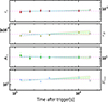 |
Fig. 17. Evolution of the derived microphysical and dynamical parameters of the afterglow of GRB 110715A for the case without IC emission. The dashed-lines in cyan and shaded regions represent results from the fit of the observed temporal evolution (open data points were left out from the fit). The horizontal pink dashed-line shows the average value for each parameter. EK, iso is in units of 1052 erg. |
The ratio ϵe/ϵB > 590 implies that SSC could be important. However, including SSC in the derivation of the parameters, we obtain an unphysical ϵB ≈ 10. We therefore assume that SSC was not relevant during the six analysed epochs presented here.
The measured microphysical and dynamical parameters were used to derive the half-opening angle θ0 of the collimated outflow, the magnitude of the magnetic field B (B = (32πmpc2n)1/2γ ; Sari et al. 1996 ) in the shock region, and the efficiency of conversion of the kinetic energy η (Table 7). Interestingly, B is evolving with α = –0.77 ± 0.04, consistent with theoretical evolution of −0.75 (see Sect. 4.2.3). The values for the efficiency are of the order of 19% which is just within the expected range of values 10%–20% (Mochkovitch et al. 1995; Kobayashi et al. 1997). The collimation angle θ0 is about 0.17 rad, which implies a total energy in the jet after the beaming correction, of Ejet = 2.27 × 1051 erg.
Energy efficiency, magnetic field magnitude, mass loss rate, and opening angle for the GRB 110715A afterglow.
3.3.2.3. Overall picture.
(a) The ooling regime is ‘slow’ cooling throughout. (b) The CMB profile is a stellar wind-like density profile. (c) The break frequency evolution is shown in Fig. 11 and consistent with evolution in wind environment. (d) The light curve plateau seen in X-rays and optical is best explained with an energy injection phase with q = –0.36 ± 0.15. The preferred model for the energy injection component is a stratification of the mass shells. (e) The observed light curve break at the end of the plateau phase coincides with a jet break of a uniform, non-spreading jet. (f) The energetics is described by a total energy in the outflow after beaming correction of Ejet = 2.27 × 1051 erg. (g) The emission mechanism is pure synchrotron.
3.3.2.4. Comparison with literature.
Sánchez-Ramírez et al. (2017) prefer an interpretation with p = 1.8 and a wind termination shock with no energy injection, which (as explicitly mentioned) does not fit the flat part at 0.3 days. We explain this feature with energy injection.
3.3.3. GRB 121024A
GRB 121024A has been already analysed in a similar way of analysis procedure (Varela et al. 2016). Thus, for the discussion in the following section, we only provide the overall picture as a summary here.
3.3.3.1. Overall picture.
(a) The cooling regime is ‘slow’ cooling throughout. (b) The CMB profile is a stellar wind-like density profile. (c) The electron spectrum is hard with a spectral index of p = 1.73 ± 0.03, and the break frequency evolution is consistent with evolution in wind environment. (d) The observed light curve break at 49.8 ± 5.1 ks is due to the jet break. (e) The energetics is described with a total energy in the outflow after the beaming correction of Ejet = 0.4 × 1051 erg. (f) The Emission mechanism is pure synchrotron.
3.3.4. GRB 130418A
3.3.4.1. Closure relations.
The evolution of the break frequencies (Fig. 15) allowed us to unambiguously identify their physical origin (see Table 3). In addition, we note that (i) the spectral slope in the X-ray band βXRT is flatter than the spectral slope in the optical/NIR bands βopt, implying SSC dominance; (ii) the early decay is very slow, suggesting substantial energy injection; (iii) the rising/falling sub-millimetre light curve indicates that νsa is initially above 345 GHz and then moves towards lower values.
Taking energy injection into account, the combination of the temporal and SED information by means of the closure relations leads to the following two options: (i) The optical data are consistent with either νc < νopt and ISM or stellar wind-like density profile (and injection parameter q = 0.14 ± 0.10) or νopt < νc and ISM (q = 0.09 ± 0.08). (ii) The X-ray data suggest either νXRT < νc and wind (q = 0.88 ± 0.16) or νXRT < νc for either stellar wind-like or ISM. Since νopt should lie in the same segment as νXRT in order to have a reasonable electron index p, the above option 1) is preferred, i.e. the cooling frequency νc lies below the NIR band during all three epochs (see Table 3 for the full parameters, and Fig. 14). Consequently, the electron index is p = 2.32 ± 0.14 as derived from the SED above νc. The evolution of the break frequencies νc and νm (Fig. 15) follows temporal slopes of α = 0.61 ± 0.03 (just marginally consistent with the expected 0.5), and α = –1.45 ± 0.06 (in perfect agreement with the theoretical value of α = –1.5), respectively. The injection parameter q = 0.14 ± 0.10 is in agreement with both, stratified mass shells, with parameter s ∼ 4.2 in a stellar wind-like density profile, and a magnetar model with an emission dominated by a Poynting flux that requires q ∼ 0.
Energy efficiency, magnetic field magnitude, mass loss rate, and opening angle for the GRB 130418A afterglow.
IC lowers the initial value of νc by a factor of (1+Y)−2 and changes the observed flux evolution to α = 1.39 when it is the dominant cooling effect. It also flattens the spectral slope above νc with an expected β = 1/3, which is in complete agreement with the observations. The first break in the optical light curve is therefore associated with the end of an energy injection phase. The second break is an achromatic break consistent with a uniform non-spreading jet. The sub-millimetre and radio data confirm that νc < νopt and the evolution of the jet is in a stellar wind-like density profile. The density normalisation A* (47) is quite possible for a Wolf-Rayet star, and in perfect agreement with the A* > 10 requirement for IC scattering being the dominant cooling process (Sari & Esin 2001).
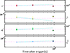 |
Fig. 18. Evolution of the derived microphysical and dynamical parameters of the afterglow of GRB 130418A without IC. The dashed lines in cyan represent the results from the fit of the observed temporal evolution, although this is only the connection of two points, since the last epoch only has limits. When considering the uncertainties, all parameters are consistent with having no evolution with time. The horizontal dashed purple lines shows the average value for each parameter. EK, iso is in units of 1052 erg. |
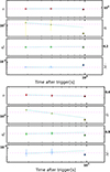 |
Fig. 19. Evolution of the energy efficiency, η; magnetic field, B; mass loss rate, Ṁ; and opening angle, θ0, derived from the measured microphysical and dynamical parameters of the afterglow of GRB 130418A with (top) and without (bottom) IC included. The dashed lines represent the results from the fit of the observed temporal evolution. Dashed pink lines show the average of each parameter. |
3.3.4.2. Afterglow parameters.
Using the measured break frequencies (Table 3) we derived the microphysical and dynamical parameters, i.e., ϵB, ϵe, EK, iso, A* (Table 8). The energy injection phase ended by the time of the first break in the light curve at tb1 = 18.8 ± 3.5 ks and the break of the non-spreading jet is at tb2 = 61.7 ± 8.1 ks. Therefore, the effect of the energy injection is not included in the derivation of the parameters, but the effect of the geometrical jet is included as a renormalisation of the peak flux to account for the difference with the expected spherical flux. When the derivation of the microphysical and dynamical parameters is performed with the SSC effect included, ϵB is of order 103, which physically is not possible. Without SSC (Fig. 18), ϵe and ϵB are less than unity, consistent with theory. The value for ϵB implies a large seed magnetic field in the CBM (Fig. 19) of order of mG (Table 9, see sect. 4.2.3). However, as expected by theory and needed by the early time observations, SSC was a dominant effect during the first stages of the afterglow evolution, with clearly observed signatures in GRB 130418A: νsa has larger values than usually expected, i.e. above sub-millimetre frequencies rather than being closer to radio frequencies, and the cooling break νc has lower values than commonly observed.
Main features for the four studied GRB afterglows.
Parameter summary of the four GRBs.
3.3.4.3. Overall picture.
(a) The cooling regime is ‘slow’ cooling throughout. (b) The CMB profile is a stellar wind-like density profile. (c) The break frequency evolution is shown in Fig. 15 and consistent with evolution in wind environment. (d) A mild energy injection is leading to a modest decline rather than a plateau. (e) The observed second light curve break is consistent with a jet break, leading to θ0 ≈ 0.45 rad. (f) The energetics is described by an isotropic energy EK, iso of 7.70 × 1051 erg, and the total energy in the outflow after beaming correction is Ejet = 1.17 × 1051 erg. (g) The emission mechanism is synchrotron with clear SSC signature in the early afterglow phase.
3.3.4.4. Comparison with literature.
To our knowledge, no results are published in refereed journals. Thus, there is nothing to compare with.
4. Discussion
The basic features of the four GRBs analysed here are presented in Table 10 and Table 11, and in the following are placed in the context of the current state in GRB afterglow studies.
4.1. Evolution of the break frequencies
The evolution of the break frequencies νc, νm and νsa for all our GRBs is composed in Fig. 20 and Table 12. All breaks are evolving as predicted by the model during fast or slow cooling. Effects such as ISS contribution to the radio observations or IC emission are included in a systematic way. The impact of possible flares has been carefully considered which could give rise to some of the observed deviations (e.g., GRB 110715A) due to the change in the temporal slopes and the flux values.
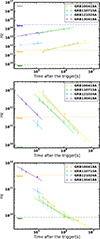 |
Fig. 20. Evolution of the break frequencies, νc (top), νm (middle) and νsa (bottom), for the afterglows of our four GRBs. The solid lines corresponds to the expected evolution of each frequency from the standard afterglow theory. The shaded regions are the fits for each break frequency. The horizontal dashed lines mark the mid-frequency for the four main observing ranges, i.e., X-rays, optical, sub-millimetre and radio. |
Temporal evolution of the measured break frequencies for our GRB afterglows. For 121024A we have only one measurement.
4.2. Fireball parameters in context
4.2.1. GRBs with all basic fireball parameters measured
For comparison purposes, we have collected those GRBs for which well-determined fireball parameters have been deduced without further assumptions (see Table C.1 and Appendix C for details). The list includes three GRBs (970508, 980703, 000926) for which different analyses have arrived at different sets of parameters, one of those even with drastically different p. We found nine GRBs with unique parameters: 3 with ISM (030329, 050904, 161219B), 5 with wind profile (060418, 090323, 090328, 140304, 181201A) preferred, and one with similarly good solutions for ISM or wind profile (140311A). All these are long-duration GRBs, as our four cases. First, we note that the addition of our 4 GRBs with well-determined fireball parameters is a worthy extension of the sample, and tips the balance towards the wind environment. More specific comparisons are made in the following sub-sections.
4.2.2. Circumburst environment
The four GRB afterglows analysed here and five of the eight clear cases in the literature are uniquely explained by a relativistic outflow expanding into a stellar wind-like density profile. In contrast, more than 50% of the GRBs from samples based on X-ray and/or optical data sets alone are associated with an ISM density profile (e.g., Panaitescu & Kumar 2002; Schulze et al. 2011; Gompertz et al. 2018). This previous dominance was surprising given the theoretical expectations for a wind-blown surrounding of massive stars and considering the relation between GRBs and Type Ic supernovae (Hjorth et al. 2003; Stanek et al. 2003; Woosley & Bloom 2006; Cano et al. 2014; Klose et al. 2019).
There are several observational biases in pinpointing the external density profile. Firstly, wavelength coverage below νc is required, since at νobs > νc there is no distinction between ISM or stellar wind-like density profiles; only at νobs < νc, the closure relations allowed us to identify the CBM profile. In the literature, X-ray samples show that for a large fraction (70–90%) of the afterglows, νXRT usually lies above νc (e.g., 22/31 GRBs; Zhang et al. 2007 and 280/300 GRBs; Curran et al. 2010). Therefore, the CBM structure cannot be determined.
Optical samples, such as the one presented in Kann et al. (2010), suggest that fewer than 25% of the afterglows (10/42) have νopt > νc if p is assumed to be larger than two. Curran et al. (2009) and Panaitescu et al. (2006) show that > 70% of their samples (ten and nine GRBs, respectively) have νobs < νc. However, they did not associate the CBM with a stellar wind-like density profile, instead they show that 1 < k < 2, as expected for an inhomogeneous density profile. In addition to these samples, about 60% of the afterglows in Greiner et al. (2011) and Schulze et al. (2011) have a break between the optical and X-ray bands, i.e., Δ β = 0.5 and/or Δα = ± 0.25 (+ISM, -stellar wind-like).
In the radio band, the peak of the light curve can be used to infer the density profile, and recent estimates resulted in more than half of the sample being consistent with ISM, 20% with wind, and the remaining 30% with 0 < k < 2 (Zhang et al. 2022).
A second problem is that in the case of using closure relations, measurement errors on α and β may not allow a conclusive statement to be made. Schulze et al. (2011) found that 22% of their afterglow sample (6 out of 27) were related to a stellar wind-like density profile, but excluded one quarter of their originally selected GRBs due to inconclusive results. The presence of breaks between νopt and νXRT may also be difficult to detect because the break is too close to an observed band, or due to the effects of  and
and  .
.
Temporal slopes (α) of the parameter change with time.
Finally, assumptions may be needed, but even if these assumptions are very plausible, they may lead to different conclusions. An illustrative example of this is seen for GRB 970228, GRB 970508, GRB 980326 and GRB 980519. Chevalier & Li (2000) associated the four afterglows with a stellar wind-like density profile, but other authors identified an ISM profile as the preferred CBM for those GRBs (e.g., Vietri 1997; Fruchter et al. 1999; Djorgovski et al. 1997; Garcia et al. 1998; Groot et al. 1998; Wang et al. 2000). The differences in the approach are partly source-specific (e.g. the sudden optical rise in 970508 after 1 day), partly due to the non-availability of the wind model in the first years after the afterglow discovery.
Summarising, the percentage of GRB afterglows associated with a stellar wind-like density profile has been increasing over the past years. However, further investigation is certainly warranted.
In a simplistic model, one could expect the wind density to scale with the mass of the Wolf-Rayet progenitor and the latter with the GRB luminosity (Hascoët et al. 2014). However, neither our four GRBs nor the sample of Table C.1 shows an obvious correlation (Fig. 21), as already suggested by Hascoët et al. (2014).
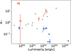 |
Fig. 21. Relation between wind density A* and the explosion luminosity (see Table C.1). Literature values are in blue, and our four GRB afterglows are in red. The grey arrows are limits as derived by Hascoët et al. (2014) for a GRB afterglow sample, with limits on the variability timescale and Lorentz factor. |
4.2.3. Microphysical parameters
The best-fit temporal slopes for each of the derived quantities, assuming a single power-law model, are given in Table 13.
For the GRBs analysed here, ϵe is constant throughout the time for all the afterglows. When looking at the absolute values, including those from the literature (Fig. C.1), substantial scatter between the GRBs can be noticed (see Fig. 22). This is in contrast to Beniamini & van der Horst (2017), who derived a narrow ϵe distribution from the analysis of the peaks of 36 radio afterglows.
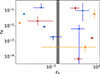 |
Fig. 22. Collection of ϵe and ϵB parameters as deduced from multi-wavelength modelling of afterglows (see Table C.1). Literature values for wind are shown in blue, orange is used for the ISM profile, and our four GRB afterglows are in red (all wind). The shaded region is the narrow ϵe distribution derived by Beniamini & van der Horst (2017). |
Interestingly, our tests for the temporal evolution of the microphysical parameters reveals a clear indication for an evolution of the magnetic field for GRBs 100418A and 130418A, see Fig. 23 and details in Table 13. Already in the early days of afterglow analysis, the effect of a non-constant ϵB on the observables was tested (Yost et al. 2003). Though these authors found a degeneracy with different external medium types, models of varying ϵB and ϵe were advocated soon after (Ioka et al. 2006; Fan & Piran 2006; Huang & Li 2023). Pretty clear observational evidence for ϵB rising with time (as t0.5) was demonstrated by Filgas et al. (2011), and Panaitescu et al. (2006) and Kong et al. (2010) have also suggested a non-constant ϵB based on observational data.
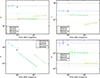 |
Fig. 23. Evolution of the secondary quantities according to the GRB afterglow standard model. The dashed-lines show the average value of each parameter. The dotted lines represent the power-law fit to the data. B has a slope −3/4 as expected from a magnetic field amplified by shock compression. θ0 is in rad, B is in G, and ṀW is in units of M⊙ yr−1. |
We recall that two possibilities were discussed for the origin of the magnetic field in GRB outflows: (i) the magnetic field is assumed to be generated by the shock from a seed that only needs to be very small in the CBM, or (ii) the blast is merely shock-compressing an existing CBM magnetic field (which is usually assumed to be of order 10 μG), as inferred for some Fermi-detected GRBs (Kumar & Barniol Duran 2009). The evolution that we find follows the predictions for a magnetic field, which originates due to shock compression, t−3/(2(4 − k)) (=t−3/4 for our case of k = 2; Blandford & McKee 1976; Rybicki & Lightman 1979; Inoue et al. 2011).
Our result is interesting for two reasons: (1) It has no additional assumptions or linked parameters among the analysed epochs of each afterglow. This implies that the observed evolution relies completely on the derived parameters for each SED and actually tests the evolution of the magnetic field in the shocked region independently. (2) Our finding of magnetic field evolution suggests shock compression as its origin. The above option (i) has been preferred because the shock compression of the pre-existing field alone would lead to a negligible magnetic energy per particle (e.g. Gruzinov 2001), and previous afterglow studies have suggested that the derived magnetic fields are about two orders of magnitude higher than the values expected from compression of the intergalactic field (Yost et al. 2003; Santana et al. 2014; Nishikawa et al. 2016). This is based on assumptions of a seed magnetic field similar to that of the Milky Way (6 μG near the Sun, up to 100 μG in some Galactic Center filaments), but there is no physical reason this applies. Based on the observation of higher magnetic fields in galaxies with large star formation rate (Beck 2012), Barniol Duran (2014) has argued that the strength of the global field might be correlated with the field in the vicinity of the GRB, thus making shock compression a viable option.
A strong relation between ϵe and the energy injection is expected. A strong energy injection affects the dynamics of the outflow and therefore the radiative processes. When the cooling process undergoes a radiative phase, ϵe is expected to be close to one (Panaitescu et al. 2006). Otherwise, if the cooling process is in an adiabatic regime, ϵe is expected to be of order 0.1 or smaller (Sari et al. 1998). At least qualitatively, we find that for the strongest injection phase, q = −0.36, the value of ϵe is larger than the other cases of energy injection (0.3).
4.2.4. Plateaus, energy injection, and more
The standard fireball model assumes an instantaneous energy injection. Observational data for many afterglows show instead that fast decays and/or plateau phases that do not follow the closure relations are commonly detected. For example, the plateau phase is part of the canonical X-ray light curve (Nousek et al. 2006; Zhang et al. 2006) having been detected in more than 50% of the X-ray afterglows.
In this study, three of the analysed GRBs have plateau phases up to 50–80 ks in the observer frame, with GRBs 100418A and 121024A also exhibiting clear optical plateaus. We have interpreted this above as prolonged energy injection (see Table 10), though this interpretation does not influence the main goal of the present work. The injection parameters (Table 14), are consistent with q > 0 (except for GRB 110715A, which is still consistent with q > 0 at 3σ, though). The observed values for the injection parameters q of our GRBs are consistent with either a mass stratification model or with a long-lived central engine with a relativistic reverse shock. The first scenario is preferred due to the lack of a convincing model for the long-lived central engine as well as the prediction for the reverse shock to dominate at early times and low frequencies, both in contrast to observations. The third injection scenario, a Poynting flux dominated outflow, is discarded for GRB 100418A with high confidence (based on the q value) and is unlikely for our other GRBs.
Spectral slopes β, injection parameter q, and electron index p for the analysed afterglows.
Besides prolonged energy injection, alternative interpretations for the common plateaus exist. One of these alternatives is forward shock emission from the edges of jet cores (Beniamini et al. 2020), with two options: (i) de-beamed emission from the core coming gradually into view, or (ii) from material travelling close to the line of sight that has not yet decelerated (this option requires a wind-like environment). Due to the strong dependence of the luminosity on the viewing angle, both interpretations can reproduce the large span of observed plateau durations and luminosities, and naturally predict a correlation between Eγ, iso, the duration of the plateau and the luminosity at the end of the plateau which is very close to the observed one. In our case, the optical emission for GRB 100418A is clearly above νm and νc during the plateau; thus both options imply an optical decay slope of 1.1, as opposed to the observed 0.36 ± 0.04. For GRB 130418A our slope errors are larger and imply consistency, while for GRB 121024A the interpretation is ambiguous given the hard p.
Another alternative interpretation is a forward shock expanding into a wind environment of particularly low density (factor 100 below typical Wolf-Rayet winds) with an unusually low Lorentz factor (of order a few tens; Dereli-Bégué et al. 2022). This scenario is not applicable to our GRBs for two reasons: first, we derive the wind normalisation A* from our data, and these are in the canonical range; second, the peak of the forward shock is constrained by public optical data (not used in our work) to be smaller than 100 s, 100 s, 60 s and 300 s, much smaller than > 104 s as expected for small A* and Γ.
4.2.5. Dynamics: EK, iso
Energy injection can have an important effect on the estimated total energy. Three of the four GRB afterglows analysed here have EK, iso of order 1052 erg or larger. GRB 110715A has the largest EK, iso, and also the largest q, i.e. the strongest energy injection. While the exact time when the deceleration (tdec) phase starts is not known, it was assumed it to be the start of the plateau phase. Combining the time of the end of the plateau phase (tinj) with T90 (as a proxy of tdec), we derive the ratio EK, iso(tdec)/ EK, iso(tinj) = (tdec/tinj)1 − q of 0.03, 0.3, 0.5 and 0.4 for GRB 100418A, 110715A, 121024A and 130418A, respectively. These ratios imply that only in the case of GRB 100418A can we assume that the initial energy is negligible (as usually assumed in the energy injection scenario), while it should not be neglected for the other GRBs. Furthermore, these ratios imply that all the efficiencies η are larger than the ones presented in Fig. 23 that were derived using EK, iso after the energy injection phase. Actually, the values for η would be 80% for GRB 100418A and 130418A, 50% for GRB 110715A and about 95% for GRB 121024A. Similar values for the ratio EK, iso(tdec)/ EK, iso(tinj) have been found by Panaitescu (2005). The increment in η was also observed in the analysis of the 31 afterglows using X-ray data presented by Zhang et al. (2007), rising up to about 90%. However, this is just a qualitative statement, as the ratios and change in η are highly dependent on the deceleration time and duration of the plateau phase.
4.3. Synchrotron self-Compton emission
Among our four GRBs, 130418A shows a clear signature of SSC emission by exhibiting βopt > βXRT, which is not possible in the standard synchrotron framework. Also, βXRT is close to the expected β = 1/3 for an SED dominated by SSC and so does the X-ray temporal slope αXRT = 1.26 that is consistent with an SSC dominated light curve when νXRT > νc. Interestingly, with A* = 45 it also matches the argument of Sari & Esin (2001) that a large value of A* (of order 10) is required to be able to detect the SSC emission directly. These findings are very similar to GRB 000926 (Harrison et al. 2001) which was among the first GRBs with direct SSC emission detection. We note in passing that hard GeV spectra seen with Fermi/LAT in some GRBs is evidence of inverse Compton emission (Panaitescu 2017).
5. Conclusions
The analysis of the broadband multi-epoch data of four GRB afterglows presented here allowed us to determine the external medium profile without ambiguity as well as all the microphysical and dynamical parameters. In the following we highlight three important results.
First, all four of the GRBs exploded into a CMB profile corresponding to a wind-blown environment. This association is consistent with the collapsar model and the GRB-SN relation. Due to the similar X-ray evolution of ISM and wind interaction, radio observations are needed to infer the CMB profile. Combined with a critical assessment of the literature, our finding suggests a larger percentage of GRBs associated with a stellar wind-like density profile than has been previously reported.
Secondly, the well-sampled multi-wavelength data allowed us to extensively test, for the first time, the temporal evolution of all synchrotron break frequencies. Consequently, we were able to test for the constancy of spectral slopes between the break frequencies and the temporal behaviour of the main physical parameters of the fireball model.
The third important result is related to the magnetic field in the shocked region. For the first time, the evolution of the magnetic field strength in the shock is derived from afterglow data, and it is found to be in agreement with the prediction of the magnetic field originating from shock amplification of the CBM magnetic field. This supports shock compression as a natural and probable origin of the shocked magnetic field. Additionally, based on the values for ϵB, the seed magnetic field in the CBM region is about 10 mG in our cases. We note that Lemoine et al. (2013) described the magnetisation as the partial decay of the micro-turbulence generated in the shock precursor and inferred such decay for four GRBs that showed extended emission at > 100 MeV.
These findings have been largely possible only due to the well-sampled broadband coverage of the afterglow emission from radio to X-rays. In particular, light curves in the radio and sub-millimetre range were key factors in deciding between different scenarios. One may suspect that when assumptions were made regarding certain parameters instead of being constrained based on observations, the previous frequent inferences of an ISM density profile could have been premature.
Based on observations collected during ESO time at the Atacama Pathfinder Experiment (APEX) under proposal 091.D-0131.
Acknowledgments
We thank the referee for helpful comments. Part of the funding for GROND (both hardware as well as personnel) was generously granted from the Leibniz-Prize to Prof. G. Hasinger (DFG grant HA 1850/28-1). KV and JG are grateful for APEX support by K. Menten, A. Weiss, and F. Bertoldi. APEX is operated by the Max-Planck Institut für Radioastronomie, the European Southern Observatory, and the Onsala Space Observatory. This work made use of data supplied by the UK Swift Science Data Centre at the University of Leicester.
References
- Aksulu, M. D., Wijers, R. A. M. J., van Eerten, H. J., & van der Horst, A. J. 2020, MNRAS, 497, 4672 [NASA ADS] [CrossRef] [Google Scholar]
- Alexander, K. D., Laskar, T., Berger, E., et al. 2017, ApJ, 848, 69 [NASA ADS] [CrossRef] [Google Scholar]
- Antonelli, L. A., Maund, J. R., Palazzi, E., et al. 2010, GRB Coordinates Network, 10620 [Google Scholar]
- Arnaud, K. A. 1996, ASP Conf. Ser., 101, 17 [Google Scholar]
- Barniol Duran, R. 2014, MNRAS, 442, 3147 [Google Scholar]
- Beck, R. 2012, Space Sci. Rev., 166, 215 [NASA ADS] [CrossRef] [Google Scholar]
- Beniamini, P., & van der Horst, A. J. 2017, MNRAS, 472, 3161 [NASA ADS] [CrossRef] [Google Scholar]
- Beniamini, P., Nava, L., Duran, R. B., & Piran, T. 2015, MNRAS, 454, 1073 [NASA ADS] [CrossRef] [Google Scholar]
- Beniamini, P., Duque, R., Daigne, F., & Mochkovitch, R. 2020, MNRAS, 492, 2847 [NASA ADS] [CrossRef] [Google Scholar]
- Berger, E., Sari, R., Frail, D. A., et al. 2000, ApJ, 545, 56 [Google Scholar]
- Berger, E., Soderberg, A. M., Frail, D. A., & Kulkarni, S. R. 2003, ApJ, 587, L5 [Google Scholar]
- Beuermann, K., Hessman, F. V., Reinsch, K., et al. 1999, A&A, 352, L26 [NASA ADS] [Google Scholar]
- Bikmaev, I., Khamitov, I., Melnikov, S., et al. 2010, GRB Coordinates Network, 10635 [Google Scholar]
- Björnsson, G., Gudmundsson, E. H., & Jóhannesson, G. 2004, ApJ, 615, L77 [CrossRef] [Google Scholar]
- Blandford, R. D., & McKee, C. F. 1976, Phys. Fluids, 19, 1130 [Google Scholar]
- Butler, N., Watson, A. M., Kutyrev, A., et al. 2013, GRB Coordinates Network, 14388 [Google Scholar]
- Cano, Z., de Ugarte Postigo, A., Pozanenko, A., et al. 2014, A&A, 568, A19 [NASA ADS] [CrossRef] [EDP Sciences] [Google Scholar]
- Cenko, S. B., Frail, D. A., Harrison, F. A., et al. 2010, ApJ, 711, 641 [Google Scholar]
- Cenko, S. B., Frail, D. A., Harrison, F. A., et al. 2011, ApJ, 732, 29 [NASA ADS] [CrossRef] [Google Scholar]
- Chambers, K. C., Magnier, E. A., Metcalfe, N., et al. 2016, ArXiv e-prints [arXiv:1612.05560] [Google Scholar]
- Chandra, P., & Frail, D. A. 2012, ApJ, 746, 156 [NASA ADS] [CrossRef] [Google Scholar]
- Chandra, P., Cenko, S. B., Frail, D. A., et al. 2008, ApJ, 683, 924 [Google Scholar]
- Chandra, P., Frail, D. A., Fox, D., et al. 2010, ApJ, 712, L31 [Google Scholar]
- Chevalier, R. A., & Li, Z.-Y. 2000, ApJ, 536, 195 [NASA ADS] [CrossRef] [Google Scholar]
- Corsi, A. 2014, GRB Coordinates Network, 17019, 1 [Google Scholar]
- Corsi, A., & Bhakta, D. R. 2014, GRB Coordinates Network, 17072, 1 [Google Scholar]
- Cucchiara, A., Veres, P., Corsi, A., et al. 2015, ApJ, 812, 122 [NASA ADS] [CrossRef] [Google Scholar]
- Curran, P. A., Starling, R. L. C., van der Horst, A. J., & Wijers, R. A. M. J. 2009, MNRAS, 395, 580 [Google Scholar]
- Curran, P. A., Evans, P. A., de Pasquale, M., Page, M. J., & van der Horst, A. J. 2010, ApJ, 716, L135 [Google Scholar]
- Dai, Z. G., & Cheng, K. S. 2001, ApJ, 558, L109 [NASA ADS] [CrossRef] [Google Scholar]
- Dai, Z. G., & Lu, T. 1998, A&A, 333, L87 [NASA ADS] [Google Scholar]
- Dai, Z. G., & Lu, T. 2000, ApJ, 537, 803 [Google Scholar]
- de Pasquale, M., Baumgartner, W. H., Beardmore, A. P., et al. 2013, GRB Coordinates Network, 14377 [Google Scholar]
- de Ugarte Postigo, A., Lundgren, A., Mac-Auliffe, F., et al. 2011, GRB Coordinates Network, 12168 [Google Scholar]
- de Ugarte Postigo, A., Lundgren, A., Martín, S., et al. 2012, A&A, 538, A44 [NASA ADS] [CrossRef] [EDP Sciences] [Google Scholar]
- de Ugarte Postigo, A., Thöne, C. C., Gorosabel, J., et al. 2013, GRB Coordinates Network, 14380 [Google Scholar]
- Dereli-Bégué, H., Pe’er, A., Ryde, F., et al. 2022, Nat. Commun., 13, 5611 [CrossRef] [Google Scholar]
- Djorgovski, S. G., Metzger, M. R., Kulkarni, S. R., et al. 1997, Nature, 387, 876 [Google Scholar]
- Duffell, P. C., & MacFadyen, A. I. 2014, ApJ, 791, L1 [CrossRef] [Google Scholar]
- Eisenstein, D. J., Weinberg, D. H., Agol, E., et al. 2011, AJ, 142, 72 [Google Scholar]
- Evans, P. A., Beardmore, A. P., Page, K. L., et al. 2007, A&A, 469, 379 [NASA ADS] [CrossRef] [EDP Sciences] [Google Scholar]
- Evans, P. A., Beardmore, A. P., Page, K. L., et al. 2009, MNRAS, 397, 1177 [Google Scholar]
- Evans, P. A., Goad, M. R., Osborne, J. P., & Beardmore, A. P. 2011, GRB Coordinates Network, 12161 [Google Scholar]
- Fan, Y., & Piran, T. 2006, MNRAS, 369, 197 [NASA ADS] [CrossRef] [Google Scholar]
- Filgas, R., Schady, P., & Greiner, J. 2010, GRB Coordinates Network, 11091 [Google Scholar]
- Filgas, R., Greiner, J., Schady, P., et al. 2011, A&A, 535, A57 [NASA ADS] [CrossRef] [EDP Sciences] [Google Scholar]
- Frail, D. A., Waxman, E., & Kulkarni, S. R. 2000, ApJ, 537, 191 [NASA ADS] [CrossRef] [Google Scholar]
- Frail, D. A., Yost, S. A., Berger, E., et al. 2003, ApJ, 590, 992 [NASA ADS] [CrossRef] [Google Scholar]
- Frail, D. A., Cameron, P. B., Kasliwal, M., et al. 2006, ApJ, 646, L99 [NASA ADS] [CrossRef] [Google Scholar]
- Fruchter, A. S., Pian, E., Thorsett, S. E., et al. 1999, ApJ, 516, 683 [Google Scholar]
- Galama, T. J., Frail, D. A., Sari, R., et al. 2003, ApJ, 585, 899 [Google Scholar]
- Gao, W.-H. 2009, ApJ, 697, 1044 [Google Scholar]
- Gao, H., Lei, W.-H., Zou, Y.-C., Wu, X.-F., & Zhang, B. 2013, New Astron. Rev., 57, 141 [CrossRef] [Google Scholar]
- Garcia, M. R., Callanan, P. J., Moraru, D., et al. 1998, ApJ, 500, L105 [Google Scholar]
- Gehrels, N., Chincarini, G., Giommi, P., et al. 2004, ApJ, 611, 1005 [Google Scholar]
- Gompertz, B. P., Fruchter, A. S., & Pe’er, A. 2018, ApJ, 866, 162 [Google Scholar]
- Gorosabel, J., Perez-Hoyos, S., Mendikoa, I., et al. 2013, GRB Coordinates Network, 14378 [Google Scholar]
- Granot, J., & Sari, R. 2002, ApJ, 568, 820 [NASA ADS] [CrossRef] [Google Scholar]
- Granot, J., Piran, T., & Sari, R. 1999, ApJ, 527, 236 [Google Scholar]
- Granot, J., Piran, T., & Sari, R. 2000, ApJ, 534, L163 [Google Scholar]
- Granot, J., Ramirez-Ruiz, E., & Loeb, A. 2005, ApJ, 618, 413 [CrossRef] [Google Scholar]
- Greiner, J., Bornemann, W., Clemens, C., et al. 2008, PASP, 120, 405 [Google Scholar]
- Greiner, J., Krühler, T., Klose, S., et al. 2011, A&A, 526, A30 [NASA ADS] [CrossRef] [EDP Sciences] [Google Scholar]
- Greiner, J., Krühler, T., Bolmer, J., et al. 2024, A&A, 691, A158 [NASA ADS] [CrossRef] [EDP Sciences] [Google Scholar]
- Groot, P. J., Galama, T. J., Vreeswijk, P. M., et al. 1998, ApJ, 502, L123 [Google Scholar]
- Gruzinov, A. 2001, ApJ, 563, L15 [Google Scholar]
- Guidorzi, C., Mundell, C. G., Harrison, R., et al. 2014, MNRAS, 438, 752 [NASA ADS] [CrossRef] [Google Scholar]
- Hancock, P. J., Murphy, T., Schmidt, B. P. G. R. B., & Coordinates, 2011, Network, 12171 [Google Scholar]
- Harrison, F. A., Yost, S. A., Sari, R., et al. 2001, ApJ, 559, 123 [Google Scholar]
- Hascoët, R., Beloborodov, A. M., Daigne, F., & Mochkovitch, R. 2014, ApJ, 782, 5 [Google Scholar]
- Hattori, T., & Aoki, K. 2010, GRB Coordinates Network, 10794 [Google Scholar]
- Higgins, A. B., van der Horst, A. J., Starling, R. L. C., et al. 2019, MNRAS, 484, 5245 [Google Scholar]
- Hjorth, J., Sollerman, J., Møller, P., et al. 2003, Nature, 423, 847 [Google Scholar]
- Huang, Y., & Li, Z. 2023, MNRAS, submitted [arXiv:2302.08230] [Google Scholar]
- Inoue, T., Asano, K., & Ioka, K. 2011, ApJ, 734, 77 [NASA ADS] [CrossRef] [Google Scholar]
- Ioka, K., Toma, K., Yamazaki, R., & Nakamura, T. 2006, A&A, 458, 7 [NASA ADS] [CrossRef] [EDP Sciences] [Google Scholar]
- Jin, Z.-P., Covino, S., Della Valle, M., et al. 2013, ApJ, 774, 114 [NASA ADS] [CrossRef] [Google Scholar]
- Jóhannesson, G., Björnsson, G., & Gudmundsson, E. H. 2006, ApJ, 647, 1238 [Google Scholar]
- Kangas, T., Fruchter, A. S., Cenko, S. B., et al. 2020, ApJ, 894, 43 [CrossRef] [Google Scholar]
- Kann, D. A., Klose, S., Zhang, B., et al. 2010, ApJ, 720, 1513 [Google Scholar]
- Klose, S., Schmidl, S., Kann, D. A., et al. 2019, A&A, 622, A138 [NASA ADS] [CrossRef] [EDP Sciences] [Google Scholar]
- Klotz, A., Gendre, B., Boer, M., et al. 2013, GRB Coordinates Network, 14382 [Google Scholar]
- Kobayashi, S. 2000, ApJ, 545, 807 [NASA ADS] [CrossRef] [Google Scholar]
- Kobayashi, S., Piran, T., & Sari, R. 1997, ApJ, 490, 92 [Google Scholar]
- Kong, S. W., Wong, A. Y. L., Huang, Y. F., & Cheng, K. S. 2010, MNRAS, 402, 409 [Google Scholar]
- Krühler, T., Küpcü Yoldaş, A., Greiner, J., et al. 2008, ApJ, 685, 376 [Google Scholar]
- Kuin, N. P. M., & de Paquale, M. 2013, GRB Coordinates Network, 14384 [Google Scholar]
- Kuin, N. P. M., & Sonbas, E. 2011, GRB Coordinates Network, 12162 [Google Scholar]
- Kumar, P., & Barniol Duran, R. 2009, MNRAS, 400, L75 [NASA ADS] [CrossRef] [Google Scholar]
- Laskar, T., Berger, E., Zauderer, B. A., et al. 2013, ApJ, 776, 119 [CrossRef] [Google Scholar]
- Laskar, T., Berger, E., Margutti, R., et al. 2015, ApJ, 814, 1 [NASA ADS] [CrossRef] [Google Scholar]
- Laskar, T., Alexander, K. D., Berger, E., et al. 2016, ApJ, 833, 88 [CrossRef] [Google Scholar]
- Laskar, T., Berger, E., Chornock, R., et al. 2018a, ApJ, 858, 65 [NASA ADS] [CrossRef] [Google Scholar]
- Laskar, T., Berger, E., Margutti, R., et al. 2018b, ApJ, 859, 134 [NASA ADS] [CrossRef] [Google Scholar]
- Laskar, T., Alexander, K. D., Berger, E., et al. 2018c, ApJ, 862, 94 [NASA ADS] [CrossRef] [Google Scholar]
- Laskar, T., van Eerten, H., Schady, P., et al. 2019, ApJ, 884, 121 [NASA ADS] [CrossRef] [Google Scholar]
- Lemoine, M., Li, Z., & Wang, X.-Y. 2013, MNRAS, 435, 3009 [NASA ADS] [CrossRef] [Google Scholar]
- Leventis, K., van Eerten, H. J., Meliani, Z., & Wijers, R. A. M. J. 2012, MNRAS, 427, 1329 [NASA ADS] [CrossRef] [Google Scholar]
- Li, Z.-Y., & Chevalier, R. A. 2001, ApJ, 551, 940 [Google Scholar]
- Marongiu, M., Guidorzi, C., Stratta, G., et al. 2022, A&A, 658, A11 [NASA ADS] [CrossRef] [EDP Sciences] [Google Scholar]
- Marshall, F. E., & Holland, S. T. 2010, GRB Coordinates Network, 10720 [Google Scholar]
- Marshall, F. E., Beardmore, A. P., Gelbord, J. M., et al. 2010, GRB Coordinates Network, 10612 [Google Scholar]
- Marshall, F. E., Antonelli, L. A., Burrows, D. N., et al. 2011, ApJ, 727, 132 [NASA ADS] [CrossRef] [Google Scholar]
- Martin, S., Petitpas, G., de Ugarte Postigo, A., et al. 2010, GRB Coordinates Network, 10630 [Google Scholar]
- Martin, S., de Ugarte Postigo, A., & Petitpas, G. 2013, GRB Coordinates Network, 14400 [Google Scholar]
- McBreen, S., Krühler, T., Rau, A., et al. 2010, A&A, 516, A71 [NASA ADS] [CrossRef] [EDP Sciences] [Google Scholar]
- Melandri, A., Kobayashi, S., Mundell, C. G., et al. 2010, ApJ, 723, 1331 [NASA ADS] [CrossRef] [Google Scholar]
- Mészáros, P., & Rees, M. J. 1997, ApJ, 476, 232 [CrossRef] [Google Scholar]
- Mochkovitch, R., Maitia, V., & Marques, R. 1995, Ap&SS, 231, 441 [NASA ADS] [CrossRef] [Google Scholar]
- Moin, A., Chandra, P., Miller-Jones, J. C. A., et al. 2013, ApJ, 779, 105 [Google Scholar]
- Nardini, M., Tanga, M., Kann, D. A., & Greiner, J. 2013, GRB Coordinates Network, 14386 [Google Scholar]
- Nelson, P. 2011, GRB Coordinates Network, 12174 [Google Scholar]
- Nishikawa, K. I., Frederiksen, J. T., Nordlund, Å., et al. 2016, ApJ, 820, 94 [NASA ADS] [CrossRef] [Google Scholar]
- Nousek, J. A., Kouveliotou, C., Grupe, D., et al. 2006, ApJ, 642, 389 [Google Scholar]
- Paczynski, B., & Rhoads, J. E. 1993, ApJ, 418, L5 [NASA ADS] [CrossRef] [Google Scholar]
- Panaitescu, A. 2005, MNRAS, 363, 1409 [Google Scholar]
- Panaitescu, A. 2017, ApJ, 837, 13 [NASA ADS] [CrossRef] [Google Scholar]
- Panaitescu, A., & Kumar, P. 2001, ApJ, 554, 667 [Google Scholar]
- Panaitescu, A., & Kumar, P. 2002, ApJ, 571, 779 [NASA ADS] [CrossRef] [Google Scholar]
- Panaitescu, A., Mészáros, P., Gehrels, N., Burrows, D., & Nousek, J. 2006, MNRAS, 366, 1357 [Google Scholar]
- Pe’er, A., & Wijers, R. A. M. J. 2006, ApJ, 643, 1036 [Google Scholar]
- Pei, Y. C. 1992, ApJ, 395, 130 [Google Scholar]
- Perley, D. A. 2013, GRB Coordinates Network, 14387 [Google Scholar]
- Perley, D. A., Cenko, S. B., Corsi, A., et al. 2014, ApJ, 781, 37 [NASA ADS] [CrossRef] [Google Scholar]
- Piranomonte, S., Vergani, S. D., Malesani, D., et al. 2011, GRB Coordinates Network, 12164 [Google Scholar]
- Quadri, U., Strabla, L., Girelli, R., & Quadri, A. 2013, GRB Coordinates Network, 14379 [Google Scholar]
- Racusin, J. L., Karpov, S. V., Sokolowski, M., et al. 2008, Nature, 455, 183 [Google Scholar]
- Racusin, J. L., Liang, E. W., Burrows, D. N., et al. 2009, ApJ, 698, 43 [NASA ADS] [CrossRef] [Google Scholar]
- Rees, M. J., & Meszaros, P. 1994, ApJ, 430, L93 [Google Scholar]
- Rees, M. J., & Mészáros, P. 1998, ApJ, 496, L1 [NASA ADS] [CrossRef] [Google Scholar]
- Resmi, L., Ishwara-Chandra, C. H., Castro-Tirado, A. J., et al. 2005, A&A, 440, 477 [NASA ADS] [CrossRef] [EDP Sciences] [Google Scholar]
- Rol, E., van der Horst, A., Wiersema, K., et al. 2007, ApJ, 669, 1098 [Google Scholar]
- Roming, P. W. A., Kennedy, T. E., Mason, K. O., et al. 2005, Space Sci. Rev., 120, 95 [Google Scholar]
- Rossi, A., Schulze, S., Klose, S., et al. 2011, A&A, 529, A142 [NASA ADS] [CrossRef] [EDP Sciences] [Google Scholar]
- Rybicki, G. B., & Lightman, A. P. 1979, Radiative processes in astrophysics (New York: Wiley) [Google Scholar]
- Sánchez-Ramírez, R., Hancock, P. J., Jóhannesson, G., et al. 2017, MNRAS, 464, 4624 [CrossRef] [Google Scholar]
- Santana, R., Barniol Duran, R., & Kumar, P. 2014, ApJ, 785, 29 [NASA ADS] [CrossRef] [Google Scholar]
- Sari, R., & Esin, A. A. 2001, ApJ, 548, 787 [NASA ADS] [CrossRef] [Google Scholar]
- Sari, R., & Mészáros, P. 2000, ApJ, 535, L33 [NASA ADS] [CrossRef] [Google Scholar]
- Sari, R., Narayan, R., & Piran, T. 1996, ApJ, 473, 204 [Google Scholar]
- Sari, R., Piran, T., & Narayan, R. 1998, ApJ, 497, L17 [Google Scholar]
- Schlafly, E. F., & Finkbeiner, D. P. 2011, ApJ, 737, 103 [Google Scholar]
- Schuller, F. 2012, SPIE Conf. Ser., 8452, 1 [Google Scholar]
- Schulze, S., Klose, S., Björnsson, G., et al. 2011, A&A, 526, A23 [NASA ADS] [CrossRef] [EDP Sciences] [Google Scholar]
- Siegel, M. H., & Marshall, F. 2010, GRB Coordinates Network, 10625 [Google Scholar]
- Siringo, G., Kreysa, E., Kovács, A., et al. 2009, A&A, 497, 945 [NASA ADS] [CrossRef] [EDP Sciences] [Google Scholar]
- Skrutskie, M. F., Cutri, R. M., Stiening, R., et al. 2006, AJ, 131, 1163 [NASA ADS] [CrossRef] [Google Scholar]
- Soderberg, A. M., Berger, E., Kasliwal, M., et al. 2006, ApJ, 650, 261 [Google Scholar]
- Soderberg, A. M., Nakar, E., Cenko, S. B., et al. 2007, ApJ, 661, 982 [Google Scholar]
- Sonbas, E., Palmer, D. M., Krimm, H. A., et al. 2011, GCN Report, 340 [Google Scholar]
- Stanek, K. Z., Matheson, T., Garnavich, P. M., et al. 2003, ApJ, 591, L17 [Google Scholar]
- Tody, D. 1993, ASP Conf. Ser., 52, 173 [NASA ADS] [Google Scholar]
- Updike, A., Rau, A., Afonso, P., & Greiner, J. 2010, GRB Coordinates Network, 10577 [Google Scholar]
- van der Horst, A. J. 2013, GRB Coordinates Network, 14434 [Google Scholar]
- van der Horst, A. J., Kamble, A. P., Wijers, R. A. M. J., et al. 2010, GRB Coordinates Network, 10647 [Google Scholar]
- van Eerten, H. 2014, MNRAS, 442, 3495 [NASA ADS] [CrossRef] [Google Scholar]
- van Eerten, H. J., & Wijers, R. A. M. J. 2009, MNRAS, 394, 2164 [Google Scholar]
- van Eerten, H., Zhang, W., & MacFadyen, A. 2010, ApJ, 722, 235 [NASA ADS] [CrossRef] [Google Scholar]
- van Marle, A. J., Langer, N., Achterberg, A., & García-Segura, G. 2006, A&A, 460, 105 [NASA ADS] [CrossRef] [EDP Sciences] [Google Scholar]
- Varela, K., van Eerten, H., Greiner, J., et al. 2016, A&A, 589, A37 [NASA ADS] [CrossRef] [EDP Sciences] [Google Scholar]
- Vietri, M. 1997, ApJ, 488, L105 [Google Scholar]
- Vlasis, A., van Eerten, H. J., Meliani, Z., & Keppens, R. 2011, MNRAS, 415, 279 [NASA ADS] [CrossRef] [Google Scholar]
- Wang, X. Y., Dai, Z. G., & Lu, T. 2000, MNRAS, 317, 170 [Google Scholar]
- Waxman, E. 1997, ApJ, 489, L33 [Google Scholar]
- Wijers, R. A. M. J., & Galama, T. J. 1999, ApJ, 523, 177 [Google Scholar]
- Wijers, R. A. M. J., Rees, M. J., & Meszaros, P. 1997, MNRAS, 288, L51 [Google Scholar]
- Woosley, S. E., & Bloom, J. S. 2006, ARA&A, 44, 507 [Google Scholar]
- Yoldaş, A. K., Krühler, T., Greiner, J., et al. 2008, Am. Inst. Phys. Conf. Ser., 1000, 227 [Google Scholar]
- Yost, S. A. 2004, Ph.D. Thesis, California Institute of Technology [Google Scholar]
- Yost, S. A., Frail, D. A., Harrison, F. A., et al. 2002, ApJ, 577, 155 [Google Scholar]
- Yost, S. A., Harrison, F. A., Sari, R., & Frail, D. A. 2003, ApJ, 597, 459 [NASA ADS] [CrossRef] [Google Scholar]
- Zhang, B., & Mészáros P. 2004, Intern. J. Mod. Phys. A, 19, 2385 [Google Scholar]
- Zhang, B., & Kobayashi, S. 2005, ApJ, 628, 315 [NASA ADS] [CrossRef] [Google Scholar]
- Zhang, B., Fan, Y. Z., Dyks, J., et al. 2006, ApJ, 642, 354 [Google Scholar]
- Zhang, B., Liang, E., Page, K. L., et al. 2007, ApJ, 655, 989 [NASA ADS] [CrossRef] [Google Scholar]
- Zhang, B., Liu, L.-D., Sun, T.-R., Lyu, F., & Wu, X.-F. 2022, ApJ, 927, 84 [Google Scholar]
Appendix A: Finding charts and photometric comparison stars
 |
Fig. A.1. GROND r′-band finding charts for GRB 100418 (left), 110715A (middle) and 130418A (right). The secondary reference stars (labelled with roman numbers) are reported in Tables A.1, A.2 and A.3, respectively. North is up, east to the left. |
Secondary stars of photometric calibration for GRB 100418A (left panel of Fig. A.1).
Secondary stars of photometric calibration for GRB 110715A (middle panel of Fig. A.1).
Secondary stars of photometric calibration for GRB 130418A (right panel of Fig. A.1).
Appendix B: Observations and data analysis
B.1. GRB 100418A
Swift.
The Swift Burst Alert Telescope (BAT) triggered and located GRB 100418A on 2010 April 18 at T0 = 21:10:08 UT (Marshall et al. 2010). Swift slewed immediately to the position of the burst, with the observations starting 79 s after the trigger with the X-ray Telescope. The afterglow was located at RA, Decl. (J2000) = 17:05:27.24, 11:27:42.7 with an uncertainty of 3.′′1. The observations started in Windowed Timing (WT) mode until T0+174 seconds followed by Photon Counting (PC) mode observations up to T0+3 Ms (Marshall et al. 2011). The Swift/XRT light curve and spectral data in the 0.3–10 keV energy range were obtained from the XRT repository (Evans et al. 2007, 2009). The Ultraviolet/Optical Telescope (UVOT; Roming et al. 2005) observed the afterglow during the same time interval as Swift/XRT. The analysis of the white filter data of the first 150 seconds located the source at RA, Decl. (J2000.0)=17:05:26.96, 11:27:41.9 with an uncertainty of 1.′′0 (Marshall et al. 2010). The observations show an initial plateau phase followed by a normal decay after T0+50 ks, with a host of magnitude 22.7 in the white band (Marshall & Holland 2010).
Optical/NIR.
GROND observations in the wavelength range from 400–2400 nm (g′r′i′z′JHKs) were targeted on the Swift/UVOT detected afterglow (Marshall et al. 2010). The observations started on April 19, 2010 at 4:50 UT (Filgas et al. 2010) and continued for 6 hours during the first night. The afterglow was detected in all 7 bands at the position RA, Decl. (J2000) = 17:05:27.09, 11:27:42.3 with an uncertainty of 0.′′4 in each coordinate (Fig. A.1). VLT/X-shooter spectroscopy of this optical afterglow revealed a redshift of z=0.623 (Antonelli et al. 2010). The GROND observations of the field of GRB 100418A continued on the 2nd, 3rd, 4th, 6th and 23rd night after the burst. The data were corrected for Galactic foreground reddening E(B − V) =0.07 mag (Schlafly & Finkbeiner 2011), corresponding to an extinction of AV =0.22 mag for Rv = 3.08.
Observed GROND magnitudes of the GRB 100418A afterglow for the seven highlighted epochs in light blue and light red in Fig. 2.
Observed magnitudes of the GRB 100418A afterglow during the epochs for the broadband analysis (as highlighted in Fig. 2).
Sub-millimetre.
The optical counterpart of GRB 100418A was followed-up in the sub-millimetre wavelength range using the Submillimeter Array SMA and the Plateau de Bure interferometer PdBI over several days.
SMA: observations of the afterglow of GRB 100418A started on April 19th 2010 at 13:00 UT, 16 hours after the trigger (Martin et al. 2010). The observations were performed at a frequency of 340 GHz with an initial detection of the counterpart with a flux of 13.40±1.60 mJy (de Ugarte Postigo et al. 2012). Follow-up observations were performed during the following 4 nights until the source was not detected any more (see Table B.3) down to a 3σ upper limit of < 4.2 mJy.
PdBI: observations started on April 19th 2010, 1.26 days after the trigger, and continued for 2 months until the source was not detected any more after 69 days down to a 3σ upper limit of < 0.57 mJy (de Ugarte Postigo et al. 2012). The observations were performed at three different bands: 86.7 GHz, 103.0 GHz and 106.0 GHz with an initial (To = 109 ks) detection at 103.0 GHz with a flux of 6.57±0.07 mJy before our chosen epochs (see Table B.3).
Sub-millimetre and radio fluxes of GRB 100418A.
Radio.
We also use published data from the Very Large Array (VLA), the Australian Telescope Compact Array (ATCA) and the Westerbork Synthesis Radio Telescope (WSRT) (Chandra & Frail 2012; de Ugarte Postigo et al. 2012; Moin et al. 2013). ATCA follow-up observation began on April 20th. The afterglow was followed for three epochs on the 2nd, 38th and 67th day after the trigger in two different bands, 5.5 GHz and 9.0 GHz (see Table B.3). WSRT observed also on April 20th, for a duration of ∼ 8 hours and detected a radio counterpart with a flux density of 369±29 μJy at a frequency of 4.8 GHz (van der Horst et al. 2010). The source was monitored at 8.46 GHz using the VLA (Moin et al. 2013) between 2 and 157 days after the trigger. It was also observed at frequencies of 4.95 GHz, 4.9 GHz and 7.9 GHz (see Table B.3).
B.2. GRB 110715A
Swift.
On 2011 July 15 at T0 = 13:13:50 UT (Sonbas et al. 2011) the Swift BAT triggered on and located GRB 110715A. Swift slewed immediately to the position of the burst, and the observations started 90 s after the trigger. The afterglow was located at RA, Decl. (J2000) = 15:50:44.07, -46:14:09.0 with an uncertainty of 2.′′2 (Evans et al. 2011). The first few thousand seconds were covered in Windowed Timing (WT) mode, during which the flux decayed with a temporal slope α of about 0.5. Photon Counting (PC) mode observations continued until T0 + 1 Ms, with two observed breaks in the light curve. The Swift/XRT light curve and spectral data were obtained from the XRT repository (Evans et al. 2007, 2009). UVOT observed the afterglow in the same time interval and located it at RA, Decl. (J2000.0) = 15:50:44.09, -46:14:06.5 with an uncertainty of 0.′′6 (Kuin & Sonbas 2011). The observations show an initial decay phase up to T0 + 22 ks, followed by a plateau phase up to T0 + 50 ks and a final decay phase.
Observed GROND magnitudes of the GRB 110715A afterglow for the epochs used in the SED analysis.
Optical/NIR.
GROND observations of the afterglow started on July 18, 2011 at 00:35 UT and continued for the next 2 hours during the first night. The afterglow was detected in all 7 bands (Updike et al. 2010) at position RA, Decl. (J2000) = 15:50:44.10, -46:14:06.2 with an uncertainty of 0.′′4 in each coordinate (Fig. A.1). VLT/X-shooter spectroscopy identified the redshift as z = 0.82 (Piranomonte et al. 2011). Observations continued on the 2nd, 4th, 6th and 8th night after the burst. The data were corrected for the Galactic foreground reddening of E(B − V)=0.59 mag (Schlafly & Finkbeiner 2011), corresponding to an extinction of  =1.82 mag for Rv = 3.08.
Sub-millimetre.
The afterglow of GRB 110715A was followed up in the sub-millimetre wavelength range using the LABOCA bolometer camera (Siringo et al. 2009) in the Atacama Path Experiment Telescope (APEX) and with the antennas of the ALMA array. It was observed at a mid-frequency of 345 GHz with both instruments, with one epoch taken with each. See Table B.5 and Fig. 9. LABOCA started observations on July 16 at 23:21 UT, observed for about 1.47 hours, and detected the source with a flux of 11.0±2.3 mJy (de Ugarte Postigo et al. 2011). ALMA observed the source 2.5 days after the detection by Swift. The source was detected with a flux of 4.9±0.60 mJy (de Ugarte Postigo et al. 2012).
Radio: ATCA.
Radio observations were performed with ATCA, starting on July 18 at 12.2 UT (Hancock et al. 2011) and continued for more than 2.5 months at four different frequencies (5.5, 9.0, 18.0, and 44.0 GHz). The observations at 9.0 GHz resulted in four detections and one upper limit. Details on the fluxes are given in Table B.5 and Fig. 9 (Chandra & Frail 2012).
Sub-millimetre and radio fluxes of GRB 110715A.
B.3. GRB 130418A
Swift.
On April 18th 2013 the Swift BAT detected GRB 130418A (de Pasquale et al. 2013) at 19:00:53 UT. Swift slewed to the position of the GRB and started observations 129.7 seconds after the trigger. The X-ray afterglow was detected by Swift/XRT at a position RA, Decl.(J2000) = 09:56:9.05, 13:39:55.4 with an uncertainty of 5.′′3. The observations were performed in Windowed Timing (WT) mode within the time interval from T0 + 136 s to T0 + 353 s, and continued in Photon Counting (PC) mode in the time interval from T0 + 3.6 ks to T0 + 407 ks. The Swift/XRT light curve and spectral data in the energy range from 0.3–10 keV were obtained from the XRT repository (Evans et al. 2007, 2009). The afterglow was also detected by the Ultraviolet/Optical Telescope (UVOT), and localised at a position of RA, Decl.(J2000) = 09:56:08.88, 13:40:02.7 with an uncertainty of 0.′′5 and a magnitude in the white band of 14.85±0.05 in the first 150 s of exposure (Kuin & de Paquale 2013).
Optical/NIR.
GROND observations of the field of GRB 130418A started on April 19, 2013 at 01:20:33 UT, 6.3 hours after the trigger (Nardini et al. 2013) and continued for the next three hours. The observations were performed simultaneous in 7 bands in a wavelength range from 400-2400 nm (g′r′i′z′JHKs). The optical counterpart was detected in all 7 bands at a position RA, Decl.(J2000) = 09:56:8.85, 13:40:02.0 with an uncertainty of 0.′′4 in each coordinate (Fig. A.1). The measured redshift is z = 1.218 (de Ugarte Postigo et al. 2013). The GROND observations continued on the third night, and in February 2014 with deep observations of the field to determine the possible host contribution. The data were corrected for Galactic foreground reddening of E(B − V) = 0.03 mag (Schlafly & Finkbeiner 2011), corresponding to an extinction of  = 0.09 mag for Rv = 3.08.
Observed GROND magnitudes of the GRB 130418A afterglow for the seven analysed epochs.
Sub-millimetre:
APEX. The afterglow of GRB 130418A was observed using the LABOCA bolometer camera (Siringo et al. 2009)3 starting on April 19th 2013 at 23:50 UT, about 22 hours after the trigger. The observations were taken in mapping mode and the reduction of the data was done using the Bolometer Array analysis software (BoA, Schuller 2012). There is an initial detection of the source with a flux of about 40 mJy with a fast decay after just a couple of hours, with a subsequent faint detection at 17 mJy. It was followed up for one the night of April 20th with no detection and a 2σ limit of 10 mJy. SMA. sub-millimetre observations were also performed using the Submillimetre Array (SMA) at Mauna Kea at a central observing wavelength of 340 GHz. The observations were performed on April 19, 2013 at 06:30 UT for 1.25 hours. No source was detected at the GRB afterglow position down to a 3σ limit of 14.5 mJy (Martin et al. 2013). CARMA. Millimetre observations using the Combined Array for Research in Millimetre-Wave Astronomy (CARMA) started observations of the field of GRB 130418A at a frequency of 93 GHz at 02:50 UT on April 19, 2013 and continued during 0.5 hours. The millimetre counterpart was detected with a flux of 3 mJy (Perley 2013).
Radio.
Radio observations of the GRB 130418A field with the WSRT were taken between April 21, 2013 13.53 UT and April 22 01.49 UT. No radio counterpart was detected with a 3σ limiting magnitude of 69 μJy (van der Horst 2013).
Appendix C: Compilation of GRBs with complete fireball parameter measurements
C.1. Selection criteria
Below, we compile all GRBs for which the afterglow modelling has allowed all five parameters (density structure, energy, ϵe, ϵB, p) to be deduced without further assumptions, such as a canonical p, energy equipartition (ϵe = ϵB = 1/3), or the location of νsa. This implicitly requires a sixth parameter to be measured, the redshift (in order to deduce proper fluxes and source-frame frequencies). In reference to earlier compilations, such as Santana et al. (2014) for ϵe and ϵB, we comment on each GRB which we deem does not fulfill our selection criterion. We admit that this selection is subjective, because many of the well-observed afterglows show deviations from the canonical behaviour, and assumptions made on these additional features might strongly influence the interpretation of the whole afterglow event. Even on a more basic level, alternative assumptions for energy injection vs. e.g. jet structure already lead to systematic differences, such as preferences for the external density profile (Panaitescu 2005). Yet, we have attempted to apply the same criteria.
The only systematic difference between our four GRBs and those compiled here is the fact that we derive the efficiency η from the final set of fireball parameters, while in general it is assumed at the onset of the analysis.
C.2. GRBs with all basic fireball parameters measured
The resulting GRBs with a complete set of fireball model parameters is summarised in Tab. C.1. We note that pre-Swift GRBs typically have very poor X-ray spectra, implying that p is only (loosely) constrained by the global model rather than the X-ray spectral slope and the knowledge of the location of the cooling break. A good example of this is GRB 980703 with two equally well fitting models but substantially different p.
GRBs with published fireball parameters, but with one or two parameters fixed at some assumed value, or other assumptions are listed with a summary of the offending detail(s):
-
971214: the ambiguity of the interpretation of the spectral break make it impossible for Wijers & Galama (1999) to constrain the physical parameters
-
980329: no redshift available; Yost et al. (2002) provide fits for z=1,2,3, and Yost et al. (2003) assume z=2
-
980519: no redshift available; Panaitescu & Kumar (2002) assume z=1 in their modelling
-
980703: Yost et al. (2003) find ISM and wind models fitting equally well, and reject the wind model based on some extreme parameter values
-
990123: Panaitescu & Kumar (2001) encounter inconsistencies re. the optical and radio decay slopes, and inclusion of energy injection or a structured jet do not solve these issues (Panaitescu 2005).
-
990510: Panaitescu & Kumar (2001) find IC to dominate, affecting νc (which is not measured), and p is inferred, as no X-ray spectral slope is used.
-
991208: the Panaitescu & Kumar (2002) modelling hinges on the interpretation of the unusual flat radio light curve during the first 10 days; Galama et al. (2003) find no explanation for the disparate slopes of the radio and optical light curves, while Li & Chevalier (2001) propose a non-standard electron energy distribution which itself is unconstrained due to the lack of X-ray observations.
-
991216: Panaitescu & Kumar (2001) find major discrepancies with the standard model, and suggest a solution with a broken power law electron distribution, having a hard p=1.2 at low energies. Energy injection is an alternative to this solution, but still does not reproduce the X-ray decline (Panaitescu 2005).
-
000301C: Li & Chevalier (2001) apply a wind model with a (non-standard) electron energy distribution which steepens with energy, while Panaitescu & Kumar (2002) require a high-energy break in the electron distribution to describe the optical data. Inclusion of energy injection or a structured jet do not solve these issues (Panaitescu 2005). Berger et al. (2000) rules out a time-varying p.
-
000418: the Panaitescu & Kumar (2002) analysis is ambiguous with respect to the CMB profile
-
010222: Panaitescu & Kumar (2002) obtain no satisfactory fit and find inconsistencies for all assumptions, see also Panaitescu (2005).
-
011211: The standard model does not fit satisfactorily, and for the structured outflow model with two more parameters the convergence of the numerical fitting is unclear (Panaitescu 2005)
-
020405: the interpretation of an early jet break hinges on two optical data points, and the strong and long-duration reverse shock(Berger et al. 2003)
-
020813: Panaitescu (2005) find no unique solution, with fireball parameters varying drastically depending on the model.
-
021004: Björnsson et al. (2004) set p=2.2, and the jet break time is set from the polarisation variation, though it is not seen in the optical light curve.
-
030226: The standard model does not fit satisfactorily, and for the structured outflow model with tregisterwo more parameters the convergence of the numerical fitting is unclear (Panaitescu 2005)
-
050416A: With νa unconstrained, Soderberg et al. (2007) assume ϵe, ϵB < 1/3
-
050820A: Cenko et al. (2010) find two alternative solutions with different p.
-
051022: Without optical detection, no distinction between ISM and wind environment is possible, and ϵe and ϵB are not well constrained (Rol et al. 2007).
-
051221: With νa unconstrained, Soderberg et al. (2006) assume ϵe, ϵB < 1/3
-
070125: Chandra et al. (2008) only find solutions (both wind and ISM) which have an isotropic-equivalent kinetic energy a factor 10 smaller than the isotropic γ-ray energy.
-
080129: Gao (2009) interpret the optical flare at 500 s after the GRB trigger with several assumptions to derive ϵe and ϵB, but neither determine p or the external density profile.
-
080319B: even with ϵB fixed at equipartition, Cenko et al. (2010) find two alternative solutions with different p, and Racusin et al. (2008) invoke a double-jetted system resulting in ϵB a factor 100 smaller.
-
080916C: Beniamini et al. (2015) assume ϵe = 0.1
-
080928: The numerical fit of a model with three energy injections does not constrain the external density profile and returns a p which is inconsistent with the X-ray and optical spectral slope (Rossi et al. 2011).
-
090423: With νa unconstrained, ϵe, ϵB and n have large uncertainties (Chandra et al. 2010)
-
090510: Beniamini et al. (2015) assume ϵe = 0.1
-
090902B: Cenko et al. (2011) find a better fit for an ISM density profile, but fix either ϵB (according to their Tab.10) or ϵe (according to their text) at the equipartition value. Beniamini et al. (2015) assume ϵe = 0.1. Lemoine et al. (2013) assume the > 100 MeV emission to be synchrotron, ignore spectral slopes, and use a two-zone model with decaying micro-turbulence to infer the fireball parameters, thus going substantially beyond the standard model.
-
090926A: Cenko et al. (2011) provide a solution for fixed ϵe = 0.33, while Beniamini et al. (2015) assume ϵe = 0.1
-
100414: Beniamini et al. (2015) assume ϵe = 0.1
-
100901A: Laskar et al. (2015) assume ϵe, ϵB < 1/3, and the interpretation hinges on the effects of the pan-chromatic re-brightening at 0.25d post-burst.
-
110625A: Beniamini et al. (2015) assume ϵe = 0.1
-
110731A: Beniamini et al. (2015) assume ϵe = 0.1. Lemoine et al. (2013) assume the > 100 MeV emission to be synchrotron, ignore spectral slopes, and use a two-zone model with decaying micro-turbulence to infer the fireball parameters, thus going substantially beyond the standard model.
-
120326A: Laskar et al. (2015) assume ϵe, ϵB < 1/3, and the interpretation hinges on the effects of the pan-chromatic re-brightening at 0.4d post-burst.
-
120404A: Guidorzi et al. (2014) interpret the pan-chromatic brightening at 0.03d as passage of νm, implying a superfast (t−12) passage, and do not fit the X-rays. Laskar et al. (2015) assume ϵe, ϵB < 1/3, and the interpretation also hinges on the effects of the pan-chromatic re-brightening.
-
130427A: Beniamini et al. (2015) assume ϵe = 0.1; due to a strong reverse shock the self-absorption frequency could not be measured, and thus ϵe, ϵB < 1/3 is assumed, leavingϵB with large uncertainties (Laskar et al. 2013; Perley et al. 2014).
-
140713A: without the detection of an optical/NIR afterglow, the modelling of Higgins et al. (2019) hinges on the association with the nearby host galaxy (and thus its redshift), and the assumption on the location of νc
-
141121A: we admire the unique solution of Cucchiara et al. (2015) for the complicated afterglow behaviour of this GRB, but we note that a Newtonian reverse shock and the allowance of different ϵB in forward and reverse shock are beyond the "standard" afterglow model, leading to our decision to not include it.
-
160131A: X-ray-to-optical and radio data separately provide good solutions, respectively, but with ϵB differing by a factor of 100, thus not allowing for a unique solution (Marongiu et al. 2022).
-
160509A: νsa is not constrained, and the radio data cannot be fit with BOXFIT nor analytically. While Kangas et al. (2020) listed a complete parameter set, the errors provided in a footnote suggest that neither E nor n are constrained. The independent measurement of extinction and IR fluxes by Kangas et al. (2020) make the Laskar et al. (2016) model incompatible with the IR data.
-
160625B: νsa is not constrained and p is inconsistent with the X-ray spectral slope (Kangas et al. 2020). Alexander et al. (2017) assume ϵe, ϵB < 1/3.
Gamma-ray bursts with measurements of all fireball parameters.
All Tables
Break frequencies for the eight epochs of the GRB 100418A afterglow using a double broken power-law.
Break frequencies for the six epochs of GRB 110715A using broadband observations.
Derived microphysical and dynamical parameters for the GRB 100418A afterglow from the five epochs of slow cooling.
Energy efficiency, magnetic field magnitude, mass loss rate, and opening angle for the GRB 110715A afterglow.
Energy efficiency, magnetic field magnitude, mass loss rate, and opening angle for the GRB 130418A afterglow.
Temporal evolution of the measured break frequencies for our GRB afterglows. For 121024A we have only one measurement.
Spectral slopes β, injection parameter q, and electron index p for the analysed afterglows.
Secondary stars of photometric calibration for GRB 100418A (left panel of Fig. A.1).
Secondary stars of photometric calibration for GRB 110715A (middle panel of Fig. A.1).
Secondary stars of photometric calibration for GRB 130418A (right panel of Fig. A.1).
Observed GROND magnitudes of the GRB 100418A afterglow for the seven highlighted epochs in light blue and light red in Fig. 2.
Observed magnitudes of the GRB 100418A afterglow during the epochs for the broadband analysis (as highlighted in Fig. 2).
Observed GROND magnitudes of the GRB 110715A afterglow for the epochs used in the SED analysis.
Observed GROND magnitudes of the GRB 130418A afterglow for the seven analysed epochs.
All Figures
|
Fig. 1. X-ray light curve of GRB 100418A from the XRT repository. The best fit is a smoothly double broken power-law shown in dashed lines. The epochs used are marked by vertical shaded regions: the steep decay phase (white), the plateau phase (blue), and the post-energy injection phase after a jet break (light green). |
| In the text | |
|
Fig. 2. GROND light curve g′r′i′z′JHKs of the afterglow of GRB 100418A. The best fit of the combined optical/NIR and X-ray data is a smooth broken power-law with host contribution shown in dash lines. The epochs used for the spectral analysis are highlighted with the vertical bars. The first two epochs highlighted in light red correspond to the energy injection phase. The last five epochs in orange correspond to the slow cooling regime, the earlier epochs to fast cooling (see Sect. 3.3.1). For the blue epochs joint GROND-XRT SEDs were produced (see Fig. 4 and Sect. 3.2.1). The green and orange epochs correspond to the SED analysis that includes radio data (Sect. 3.3). |
| In the text | |
|
Fig. 3. Sub-millimetre and radio light curves of the GRB 100418A afterglow at different frequencies. Dashed lines show the best fit. The eight highlighted vertical regions correspond to the epochs used in the SED analysis. The orange (blue) regions correspond to the fast (slow) cooling regime. The light curves were scaled by an arbitrary factor for clarity. |
| In the text | |
|
Fig. 4. Spectral energy distributions of the afterglow of GRB 100418A using GROND and XRT data at five epochs: SED1 (t = 130.9 ks), SED2 (t = 202.1 ks), SED3 (t = 217.8 ks), SED4 (t = 296.8 ks), and SED5 (t = 476.4 ks). For clarity, the SEDs were scaled arbitrarily (GROND magnitudes are given in Table B.1). The best-fit SED slope is β = 1.11 ± 0.02. |
| In the text | |
|
Fig. 5. Broadband SED analysis for GRB 100418A using eight epochs analysed using multi-epoch broadband observations. The first three epochs correspond to the fast cooling regime (SED1r – SED3r); the last five epochs (SED4r – SED8r) correspond to the slow cooling regime. The best-fit model for all SEDs is a double broken power-law with smooth breaks. |
| In the text | |
|
Fig. 6. Evolution of the measured break frequencies for the eight optical to radio SEDs for the GRB 100418A afterglow. The solid lines represent the expected theoretical evolution for a wind environment during fast (< 600 ks) and slow (> 600 ks) cooling. The coloured dashed lines represent the best power-law fits to the measured temporal evolution (open data points were left out from the fit). The horizontal dashed lines show the mean frequencies of our data (X-ray, optical, sub-millimetre, radio). |
| In the text | |
|
Fig. 7. X-ray light curve of the GRB 110715A afterglow described by a smooth double broken power-law shown in dashed lines. The three regions used in the SED analysis are shown as shaded areas, corresponding to the GRB tail, the plateau and the final decay phase, respectively. |
| In the text | |
|
Fig. 8. GROND g′r′i′z′JHKs light curve of the GRB 110715A afterglow. The best fit is a single power-law with α = 1.51 ± 0.03, as shown with the dashed lines. The epochs used for the spectral analysis are highlighted with the vertical bars. All four epochs are after the plateau phase. |
| In the text | |
|
Fig. 9. Sub-millimetre and radio light curves of the GRB 110715A afterglow. The best fit for each of the bands is represented by dashed lines. The six highlighted vertical regions correspond to the epochs used in the broadband multi-epoch SED analysis. The light curves were scaled by an arbitrary factor for clarity. |
| In the text | |
|
Fig. 10. Broadband analysis of the GRB 110715A afterglow. Six epochs are presented with all the breaks measured. |
| In the text | |
|
Fig. 11. Evolution of the break frequencies of the afterglow of GRB 110715A. The last SED is not included in the fit because the values for the optical/NIR bands were extrapolated. Lines are as in Fig. 6. |
| In the text | |
|
Fig. 12. X-ray light curve of the afterglow of GRB 130418A with the early WT data omitted. The highlighted vertical regions corresponds to the two main epochs of the SED analysis. |
| In the text | |
|
Fig. 13. Optical/NIR light curve of the afterglow of GRB 130418A observed with GROND, including data from the literature. The best-fit model is a double broken power-law with smooth breaks, and includes a host detection at r′(AB) = 25.4 ± 0.3 mag. |
| In the text | |
|
Fig. 14. Broadband SEDs of the GRB 130418A afterglow at the three epochs of Table 3. Data are given in Table B.6. |
| In the text | |
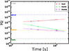 |
Fig. 15. Evolution of the break frequencies of the GRB 130418A afterglow. Lines are as in Fig. 6. |
| In the text | |
|
Fig. 16. Slow cooling: Evolution of the derived dynamical (top) and microphysical (bottom) parameters of the afterglow of GRB 100418A without SSC emission. The blue dashed lines and shaded regions represent the results from the fit of the observed temporal evolution. The horizontal dashed purple lines show the average value for each parameter. EK, iso is in units of 1052 erg. |
| In the text | |
|
Fig. 17. Evolution of the derived microphysical and dynamical parameters of the afterglow of GRB 110715A for the case without IC emission. The dashed-lines in cyan and shaded regions represent results from the fit of the observed temporal evolution (open data points were left out from the fit). The horizontal pink dashed-line shows the average value for each parameter. EK, iso is in units of 1052 erg. |
| In the text | |
|
Fig. 18. Evolution of the derived microphysical and dynamical parameters of the afterglow of GRB 130418A without IC. The dashed lines in cyan represent the results from the fit of the observed temporal evolution, although this is only the connection of two points, since the last epoch only has limits. When considering the uncertainties, all parameters are consistent with having no evolution with time. The horizontal dashed purple lines shows the average value for each parameter. EK, iso is in units of 1052 erg. |
| In the text | |
|
Fig. 19. Evolution of the energy efficiency, η; magnetic field, B; mass loss rate, Ṁ; and opening angle, θ0, derived from the measured microphysical and dynamical parameters of the afterglow of GRB 130418A with (top) and without (bottom) IC included. The dashed lines represent the results from the fit of the observed temporal evolution. Dashed pink lines show the average of each parameter. |
| In the text | |
|
Fig. 20. Evolution of the break frequencies, νc (top), νm (middle) and νsa (bottom), for the afterglows of our four GRBs. The solid lines corresponds to the expected evolution of each frequency from the standard afterglow theory. The shaded regions are the fits for each break frequency. The horizontal dashed lines mark the mid-frequency for the four main observing ranges, i.e., X-rays, optical, sub-millimetre and radio. |
| In the text | |
|
Fig. 21. Relation between wind density A* and the explosion luminosity (see Table C.1). Literature values are in blue, and our four GRB afterglows are in red. The grey arrows are limits as derived by Hascoët et al. (2014) for a GRB afterglow sample, with limits on the variability timescale and Lorentz factor. |
| In the text | |
|
Fig. 22. Collection of ϵe and ϵB parameters as deduced from multi-wavelength modelling of afterglows (see Table C.1). Literature values for wind are shown in blue, orange is used for the ISM profile, and our four GRB afterglows are in red (all wind). The shaded region is the narrow ϵe distribution derived by Beniamini & van der Horst (2017). |
| In the text | |
|
Fig. 23. Evolution of the secondary quantities according to the GRB afterglow standard model. The dashed-lines show the average value of each parameter. The dotted lines represent the power-law fit to the data. B has a slope −3/4 as expected from a magnetic field amplified by shock compression. θ0 is in rad, B is in G, and ṀW is in units of M⊙ yr−1. |
| In the text | |
|
Fig. A.1. GROND r′-band finding charts for GRB 100418 (left), 110715A (middle) and 130418A (right). The secondary reference stars (labelled with roman numbers) are reported in Tables A.1, A.2 and A.3, respectively. North is up, east to the left. |
| In the text | |
Current usage metrics show cumulative count of Article Views (full-text article views including HTML views, PDF and ePub downloads, according to the available data) and Abstracts Views on Vision4Press platform.
Data correspond to usage on the plateform after 2015. The current usage metrics is available 48-96 hours after online publication and is updated daily on week days.
Initial download of the metrics may take a while.