| Issue |
A&A
Volume 701, September 2025
|
|
|---|---|---|
| Article Number | A113 | |
| Number of page(s) | 23 | |
| Section | Extragalactic astronomy | |
| DOI | https://doi.org/10.1051/0004-6361/202554797 | |
| Published online | 09 September 2025 | |
MIRACLE
I. Unveiling the multi-phase, multi-scale physical properties of the active galaxy NGC 424 with MIRI, MUSE, and ALMA
1
Dipartimento di Fisica e Astronomia, Università degli Studi di Firenze, Via G. Sansone 1, I-50019 Sesto Fiorentino, Firenze, Italy
2
INAF – Osservatorio Astrofisico di Arcetri, Largo E. Fermi 5, I-50125 Firenze, Italy
3
University of Trento, Via Sommarive 14, Trento, I-38123, Italy
4
Scuola Normale Superiore, Piazza dei Cavalieri 7, Pisa I-56126, Italy
5
Centro de Estudios de Física del Cosmos de Aragón (CEFCA), Plaza San Juan 1, 44001 Teruel, Spain
6
Istituto di Astrofisica e Planetologia Spaziali (INAF-IAPS), Via Fosso del Cavaliere 100, 00133 Roma, Italy
7
Instituto de Radioastronomía y Astrofísica, UNAM, Campus Morelia, A.P. 3-72, C.P. 58089, Mexico
8
ESO, Karl-Schwarzschild-Str 2, D-85748 Garching bei München, Germany
9
Instituto de Astrofísica de Canarias, 38205 La Laguna, Tenerife, Spain
10
Departamento de Astrofísica, Universidad de La Laguna, 38206 La Laguna, Tenerife, Spain
11
Institute for Physics, Laboratory for Galaxy Evolution and Spectral Modelling, Ecole Polytechnique Federale de Lausanne, Observatoire de Sauverny, Chemin Pegasi 51, CH-1290 Versoix, Switzerland
12
INAF, Osservatorio Astronomico di Trieste, Via Tiepolo 11, I-34131 Trieste, Italy
13
AURA for ESA, Space Telescope Science Institute, 3700 San Martin Drive, Baltimore, MD 21218, USA
14
Departamento de Física, Universidad Técnica Federico Santa María, Vicuña Mackenna 3939, San Joaquín, Santiago de Chile, Chile
15
IFPU – Institute for Fundamental Physics of the Universe, via Beirut 2, I-34151 Trieste, Italy
16
Max-Planck-Institut für extraterrestrische Physik (MPE), Gießenbachstraße 1, 85748 Garching, Germany
17
Observatorio Astronómico Nacional, C/ Alfonso XII 3, E-28014 Madrid, Spain
18
Dipartimento di Fisica e Astronomia, Alma Mater Studiorum, Università degli Studi di Bologna, Via Gobetti 93/2, 40129 Bologna, Italy
19
INAF–Osservatorio di Astrofisica e Scienza dello Spazio di Bologna, Via Gobetti 93/3, 40129 Bologna, Italy
20
Department of Physics, University of Arkansas, 226 Physics Building, 825 West Dickson Street, Fayetteville, AR 72701, USA
⋆ Corresponding author This email address is being protected from spambots. You need JavaScript enabled to view it.
Received:
27
March
2025
Accepted:
17
July
2025
Abstract
We present an analysis of the multi-phase gas properties in the Seyfert II galaxy NGC 424, using spatially resolved spectroscopic data from JWST/MIRI, part of the Mid-InfraRed Activity of Circumnuclear Line Emission (MIRACLE) programme, as well as VLT/MUSE and ALMA. We traced the properties of the multi-phase medium, from cold and warm molecular gas to hot ionised gas, using emission lines such as CO (2-1), H2S(1), [O III]λ5007, [Ne III]15.55μm, and [Ne V]14.32μm. These lines reveal the intricate interplay between the different gas phases within the circumnuclear region, spanning a maximum scale of 7 × 7 kpc2 and a spatial resolution of 110 pc, with MUSE and ALMA, respectively. Exploiting the multi-wavelength and multi-scale observations of gas emission, we modelled the galaxy disc rotation curve from scales of a few parsec up to ∼5 kpc from the nucleus and inferred a dynamical mass of Mdyn = (1.09 ± 0.08) × 1010 M⊙ with a disc scale radius of RD = (0.48 ± 0.02) kpc. We detected a compact ionised outflow with velocities up to 103 km s−1, traced by the [O III], [Ne III], and [Ne V] transitions, with no evidence of cold or warm molecular outflows. We suggest that the ionised outflow might be able to inject a significant amount of energy into the circumnuclear region, potentially hindering the formation of a molecular wind, as the molecular gas is observed to be denser and less diffuse. The combined multi-band observations also reveal, mainly in the ionised and cold molecular gas phases, a strong enhancement of the gas velocity dispersion directed along the galaxy minor axis, perpendicular to the high-velocity ionised outflow, and extending up to 1 kpc from the nucleus. Our findings suggest that the outflow might play a key role in such an enhancement by injecting energy into the host disc and perturbing the ambient material.
Key words: galaxies: active / galaxies: ISM / galaxies: kinematics and dynamics / galaxies: Seyfert
© The Authors 2025
 Open Access article, published by EDP Sciences, under the terms of the Creative Commons Attribution License (https://creativecommons.org/licenses/by/4.0), which permits unrestricted use, distribution, and reproduction in any medium, provided the original work is properly cited.
This article is published in open access under the Subscribe to Open model. This email address is being protected from spambots. You need JavaScript enabled to view it. to support open access publication.
1. Introduction
Active galactic nuclei (AGNs) are widely recognised as fundamental drivers of galaxy evolution through the AGN feedback process. The energy released by gas accretion onto supermassive black holes (SMBHs) can generate powerful winds and outflows that propagate through the host galaxy, influencing the surrounding interstellar medium (ISM). AGN-driven outflows are now considered a key mechanism for regulating star formation and shaping the overall mass distribution in galaxies (e.g. Fabian 2012; Kormendy & Ho 2013; King & Pounds 2015; Cicone et al. 2018; Harrison et al. 2018)
Outflows driven by AGNs are inherently multi-phase, comprising gas in the ionised, atomic, and molecular states, each contributing differently to feedback processes. Ionised outflows, often traced by optical emission lines like [O III]λ5007, can reach velocities of several hundred to a few thousand kilometres per seconds, transporting warm (T ∼ 104 K), low-density gas (Ne ∼ 102 − 4 cm−3) out of the nucleus and up to kiloparsec scales (e.g. Carniani et al. 2015; Bae & Woo 2016; Woo et al. 2016; Fiore et al. 2017; Cicone et al. 2018; Venturi et al. 2018, 2021; Harrison et al. 2018; Cresci et al. 2023). These outflows are critical in dispersing gas from the nuclear regions, though their efficiency in quenching star formation is still debated both in observations and simulations (see e.g. Cresci et al. 2015; Balmaverde et al. 2016; Zubovas & Bourne 2017; Combes 2017; Mulcahey et al. 2022; Piotrowska et al. 2022; Belli et al. 2024). Molecular outflows, on the other hand, represent colder, denser phases of gas and are frequently observed via CO transitions. They are typically slower, with velocities of the order of a few hundred km s−1, but can carry a substantial amount of mass (Mout ∼ 107–109 M⊙) and are possibly more directly involved in regulating star formation (e.g. Feruglio et al. 2010; Fiore et al. 2017; Carniani et al. 2015; García-Burillo et al. 2019; Fluetsch et al. 2019).
Understanding the energetics of these outflows – specifically their mass outflow rates, momentum, and energy flux – is essential for constraining their impact on galactic scales. Recent studies have shown that the coupling efficiency between the SMBH and the surrounding gas can vary depending on the phase of the outflow. Indeed, although the cold molecular phase carries the bulk of the outflowing gas mass, the kinetic energies are higher in the ionised phase (Rupke et al. 2017; Vayner et al. 2021; Riffel et al. 2023; Harrison & Ramos Almeida 2024). Multi-phase outflows are thus a key feature of AGN feedback, as they link the energetic output of the AGN to the ambient ISM across a wide range of temperatures and densities (e.g. Rupke & Veilleux 2013; Cazzoli et al. 2018).
Recent high-resolution observations from facilities such as the Atacama Large Millimeter Array (ALMA; Wootten & Thompson 2009) have investigated the role of cold molecular outflows in AGNs, showing that this gas phase can be accelerated to high velocities and can extend across several kiloparsecs (Fluetsch et al. 2019). Additionally, ionised outflows are a ubiquitous manifestation of AGN feedback, mainly traced through optical emission lines such as and Hα (e.g. Harrison et al. 2014; Fiore et al. 2017). Finally, warm molecular outflows (T = 10 − 102 K, ne ≥ 103 cm−3) are typically traced by roto-vibrational transitions of H2 in the near-infrared regime using instruments such as the Spectrograph for INtegral Field Observations in the Near-Infrared (SINFONI; Eisenhauer et al. 2003) or the Near-Infrared Spectrograph on board JWST (NIRSpec; Jakobsen et al. 2022) and in the mid-infrared (MIR) using Spitzer and more recently JWST (Wright et al. 2023) mid-infrared observations. H2 emission is both observed and predicted to be particularly rich in shocked gas, and therefore represents a valuable tracer of warm molecular outflowing gas (Hill & Zakamska 2014; Richings & Faucher-Giguère 2018a,b; Riffel et al. 2020). Thus, the role of multi-phase outflows spans from the circumnuclear scale up to galactic scales, since they can sweep away the ambient material and also affect the conditions of the host halo, potentially halting cooling flows and limiting the accretion of new gas onto the galaxy.
In addition to their feedback potential, multi-phase outflows provide important clues about the physics of gas accretion and ejection around SMBHs. The co-existence of gas in very different physical conditions, ranging from ionised, high-temperature plasma to cold molecular clouds, indicates that AGN-driven winds may entrain gas from different regions of the ISM or cool as they propagate outwards (Zubovas et al. 2024). This entrainment process allows molecular gas to survive in extreme environments, where heating from shocks and radiation fields might otherwise be expected to dissociate or ionise the gas (Richings & Faucher-Giguère 2018a; Chen & Oh 2024). Studying these outflows in detail, and in particular with a high spatial resolution, is therefore crucial for understanding how energy is transferred across the ISM and how AGN feedback can shape the evolution of galaxies (Ward et al. 2024; Sivasankaran et al. 2025; Byrne et al. 2024).
Recent JWST/MIRI (Rieke et al. 2015b) observations have already started to revolutionise our comprehension of the MIR activity of local AGNs by allowing integral field spectroscopy (IFS) to be conducted in this spectral region (García-Bernete et al. 2022; Armus et al. 2023; Bajaj et al. 2024). Indeed, the exceptional sensitivity and spatial resolution of the Medium-Resolution Spectrometer (MRS, Labiano et al. 2021) allow us to detect high-ionisation transitions such as [Ne V]14.3μm, [Ne V]24.3μm, and [O IV]25.8μm, which is proving to be crucial for probing the AGN activity in the circumnuclear region (Lai et al. 2022; Zhang et al. 2024; Riffel et al. 2025) thanks to the nearly unbiased view through dust attenuation (Gordon et al. 2023; García-Bernete et al. 2024; Donnan et al. 2024). This breakthrough capability is pivotal for unveiling the intricate interplay between the AGN radiation field and the circumnuclear ambient medium. Moreover, combining the Mid-Infrared Instrument MRS with the optical Multi Unit Spectroscopic Explorer (MUSE) at the ESO Very Large Telescope (VLT; Bacon et al. 2010) and the sensitivity and spatial resolution in the millimetre regime of ALMA paves the way for a complete characterisation of the multi-phase properties of galactic outflows. In particular, the synergy among these facilities enables us to simultaneously trace the ionised, warm, and cold gas components, offering a holistic view of the feedback processes regulating the star formation and driving the galaxy evolution. Such a multi-wavelength and multi-scale approach marks a significant step forwards in our ability to disentangle the complex mechanisms governing AGN-driven outflows and their impact on the host galaxy.
In this paper, we present the first data of our Mid-InfraRed Activity of Cicumnuclear Line Emission (MIRACLE; PID: 6138, Co-PIs: C. Marconcini and A. Feltre) programme, aimed at observing a sample of seven nearby AGNs in the 5–28 μm wavelength range with the MIRI MRS on board the JWST telescope. This project leverages the large spectral coverage of MIRI in MRS mode that grants access to a plethora of low- to high-ionisation atomic emission lines and rotational transitions of H2. We aim to map the gas ionisation source, kinematics, and morphology for each gas phase, exploiting modern suites of photoionisation and kinematic models. Finally, we aim to characterise the interplay between different gas flow phases, the AGN, and the host galaxy at similar spatial resolutions, constraining the gas flow energetics and impact on the ambient gas.
This paper focuses on a comprehensive analysis of the multi-phase gas properties in the first observed target of our programme, i.e. NGC 424, using a combination of infrared, optical, and millimetre data from MIRI on the JWST, MUSE, and ALMA, respectively. These observations allow the multi-phase gas to be traced across a wide range of temperatures and densities, providing a detailed view of its kinematics, structure, and energetics.
NGC 424 is a nearby heavily obscured Seyfert-II galaxy (z = 0.01175 ± 0.000061, D = 51 Mpc, 1″ ∼ 230 pc). It has not been studied closely in any gas phase; nevertheless, its proximity makes it an ideal target for high-resolution, multi-wavelength studies aimed at tracing the full extent of the gas properties across a wide wavelength range to understand the interplay between its different gas phases. In the X-rays, Ricci et al. (2017) estimated an intrinsic 2–10 keV X-ray luminosity of log(LX/erg s−1) = 43.77 and a column density of log(nH/cm−2) = 24.33 ± 0.01. Additionally, Kakkad et al. (2022) used archival MUSE observations to estimate the ionised outflow energetic traced by the [O III]λ5007 emission line. They found an average outflow velocity of 814 ± 70 km s−1 and a mass outflow rate of 26.3 ± 1.3 M⊙ yr−1. In this paper we present the first observations of our MIRACLE programme, providing a comprehensive energetic analysis of the multi-phase outflow across various scales in NGC 424.
This paper is organised as follows. In Section 2, we describe the observations and data reduction procedures for MIRI, MUSE, and ALMA. In Section 3 we present the data analysis for each instrument, discussing the spectroscopic analysis of specific emission lines tracing different gas phases. In Section 4 we discuss our results and present a detailed morphological and kinematic analysis of the multi-phase gas properties across different scales. In Section 5, we discuss the implications of our findings for AGN feedback and the interplay among different gas phases. Finally, in Section 6 we summarise our findings.
2. Observations and data reduction
We combined new observations of NGC 424 obtained with the MRS as part of the MIRACLE survey (Marconcini et al., in prep.) with archival observations from VLT/MUSE and ALMA. The field of view (FoV) covered by each instrument is shown in Fig. 1. The observations and data reduction pipeline adopted for each telescope are discussed in the following sections.
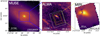 |
Fig. 1. NGC 424 emission line images from MUSE WFM (left), ALMA (middle), and the point-source subtracted MIRI MRS Ch3 medium (right). The images were obtained integrating the total [O III]λ5007, CO (2-1), and [Ne V] emission lines, respectively. Blue square in MUSE image represents the ALMA FoV considered in this work. Orange, red, yellow, and white rectangles in ALMA image represent the FoVs of MIRI MRS Channels 1, 2, 3, and 4, respectively. Black crosses mark the nucleus position, determined as the peak of Hα emission from the MUSE data. North is up and east is left. |
2.1. JWST/MIRI
The JWST/MIRI observations of NGC 424 are part of the GO Cycle 3 MIRACLE programme 6138. The data were acquired with MIRI (Rieke et al. 2015a,b; Labiano et al. 2021) in MRS mode (Wells et al. 2015) on 2024 October 20 UT, using a single pointing on the source and a linked, dedicated background field. We used the MRS with all channels 1–4, covering the spectral range 4.9–28.1 μm, with three grating settings, SHORT (A), MEDIUM (B), and LONG (C), reading both the SHORT and LONG detectors in each case via the FASTR1 pattern, thus optimising the dynamic range expected in the observations. For each grating/detector configuration the science (and background) observation consisted of a single exposure per dither position, each exposure consisting of eight integrations of 25 groups. We adopted a standard four-point dither pattern to improve spatial sampling, which gives a total on-source time of 2298 s per configuration. Because our source is extended, we linked the science observation to a dedicated background with the same observational parameters in all three grating settings. We downloaded the uncalibrated science and background observations through the Barbara A. Mikulski Archive for Space Telescopes (MAST) portal and the data reduction process was performed using the JWST Science Calibration Pipeline (Bushouse et al. 2022) version 1.16.0. We applied all the three stages of the pipeline processing, which include CALWEBB_DETECTOR1, CALWEBB_SPEC2, and CALWEBB_SPEC3 (see Morrison et al. 2023; Patapis et al. 2024).
Additional fringe corrections were made during stages 2 and 3, using the standard pipeline code. The CALWEBB_DETECTOR1 pipeline corrects the raw detector ramps of each exposure for multiple electronic artefacts such as bad pixels and cosmic-rays, producing slope images with the count rate in Data Number (DN) per second in each pixel. The resulting slope images are then processed with the CALWEBB_DETECTOR2 step, where each image is corrected for distortion and then calibrated both in wavelength and flux (see Argyriou et al. 2020, 2023 for a detailed description of all the detector-level steps performed during this stage). A first residual fringe correction is applied during this stage. The results of stage 2 are calibrated slope images in units of MJy sr−1. Then, each calibrated image goes through the final CALWEBB_SPEC3 stage, which performs background subtraction to each single-exposure observation. In this work, we subtracted the background emission from the 2D science images using a spaxel-by-spaxel background frame generated from our dedicated background observations. Then, the main step of the third stage is to create the final data cubes by combining the flux-calibrated, dithered science images in a composite 3D data cube. To assemble the final data cubes, we used the exponential modified-Shepard method (EMSM) weighting function, which has proven to be more efficient in reducing the drizzling effect (Law et al. 2023) and thus improve the final output. We combined all the final data cubes on the detector plane using the skyalign orientation provided by the JWST pipeline, i.e. cubes are oriented according to the world coordinates RA, Dec. Based on these steps, the results of the pipeline process are 12 data cubes, one per each sub-band, which span progressively larger FoVs, from 3.2″ × 3.7″ in Channel 1 to 6.6″ × 7.7″ in Channel 4. Moreover, each sub-Channel data cube has a different spaxel sampling, i.e. 0.13, 0.17, 0.2, and 0.35″/pxl, from Channel 1 to Channel 4, respectively. As is discussed in Appendix A, the MIRI/MRS PSF increases its FWHM, by varying the angular resolution of the data from 0.4″ (100 pc) to 0.5″ (120 pc), 0.6″ (145 pc), 0.9″ (220 pc), in Channels 1, 2, 3, and 4, respectively. The MIRI integrated spectrum was obtained by combining the emission from the 12 reduced data cubes, taking into account the different pixel sizes, and ensuring a proper flux conservation among different bands, applying a scaling factor to align the flux levels between adjacent bands and stitch the spectra. A comprehensive description of the procedure for stitching together spectra covering different bands and accounting for variable pixel sizes and FoV is presented in Ceci et al. (2025). Finally, to investigate the spatially resolved extended emission in each band we performed a detailed point spread function (PSF) subtraction procedure to each data cube, using the WebbPSF tool (see Appendix A for moredetails).
2.2. MUSE
NGC 424 IFS archival data obtained with MUSE (ID: 095.B-0934, P.I. S. Juneau) are part of the extended Measuring AGN Under Muse (MAGNUM) sample (Cresci et al. 2015; Venturi et al. 2017, 2018; Mingozzi et al. 2019; Marconcini et al. 2023). The sample was selected by cross-matching the optically selected AGN samples of Maiolino & Rieke (1995) and Risaliti et al. (1999), and Swift-BAT 70-month Hard Xray Survey (Baumgartner et al. 2013), choosing only sources observable from Paranal Observatory (70° ≤ δ ≤ 20°) and with a luminosity distance D ≤ 50 Mpc. We retrieved the data from ESO archive2, already reduced with the standard MUSE pipeline (v1.6) and with an average PSF FWHM of 0.8″. The final data cube consists of 322 × 318 spaxels, with a spatial sampling of 0.2″ pixel−1, covering the spectral range between 4750 to 9350 Å, thus tracing the rest-frame optical wavelength range. The MUSE spectral resolution spans from 1750 at 4650 Åto 3750 at 9300 Å. The observations’ FoV of 1′ × 1′ corresponds to a region of 14 kpc × 14 kpc centred in the nucleus of NGC 424.
2.3. ALMA
To investigate the cold molecular gas phase in NGC 424, we analysed archival ALMA 12-m array band 6 observations from programme 2021.1.01150.S (P.I. A. Rojas) covering the observed spectral window of [226.91, 228.79] GHz, which allowed us to trace the CO (2-1) emission at 230.538 GHz rest-frame. For the ALMA data considered in this work, the FoV is 38″ in diameter, with the largest recoverable scale of 11.4″. We requested the calibrated measurement sets from the European ALMA Regional Centre (ARC; Hatziminaoglou et al. 2015b). To reduce and analyse the data, we used the Common Astronomy Software Applications (CASA) package version v6.1.1 (McMullin et al. 2007; CASA Team 2022). This program includes observations with two configurations, with beam sizes of 0.2″ and 1″, respectively. We combined the two measurement sets to obtain the best compromise in terms of spatial resolution and sensitivity. In particular, for the CO (2–1) spectral window, we subtracted a constant continuum level estimated from the emission line free channels in the uv plane3. The data were cleaned using the CASA task TCLEAN CASA task using a BRIGGS weighting scheme with ROBUST = 0.5, to achieve a ∼110 pc resolution (beam size FWHM 0.48″ × 0.44″, beam PA = 1°). The final reduced data cube has a spectral channel width of ∼5 km s−1, a pixel size of 90 mas, and a root mean square (RMS) of 0.94 mJy/beam per channel.
3. Data analysis
In this section we outline the general spectroscopic routine used to perform the emission line analysis of the MUSE, ALMA, and MIRI data cubes. Overall, we analysed the MIRI and MUSE data cubes using a set of tailored Python scripts in order to subtract the continuum and fit the emission lines with multiple Gaussian components where needed. Figure 2 shows the NGC 424 MUSE (top panel) and MIRI (bottom panel) integrated spectra with the detected optical and MIR emission lines, extracted from the smallest MIRI/MRS FoV (i.e. Channel 1). The total flux of each detected emission line in the MIRI/MRS spectral coverage, together with the maximum number of Gaussian components used to reproduce each line profile, are listed in Table 1. For comparison, in the bottom panel of Fig. 2 we show the Spitzer (Werner et al. 2004) Infrared Spectrometer (IRS; Houck et al. 2004) high-resolution spectrum of NGC 424 extracted in full mode (PID: 30291; P.I.: G. Fazio) and retrieved from the Combined Atlas of Sources with Spitzer IRS (CASSIS Lebouteiller et al. 2011, 2015). The Spitzer/IRS spectrum reveals the main MIR ionised transitions as well as the H2S(1) transition, together with the source MIR continuum. As is shown in the bottom panel of Fig. 2, we find evidence of polycyclic aromatic hydrocarbon (PAH) features at 11.25 and 12 μm, with a higher equivalent width (EW) with respect to the Spitzer spectrum. In particular, we performed a local continuum fit, integrated the PAH flux, and estimated EW11μm = 0.007 μm, and EW12μm = 0.01 μm, for the PAH features at 11.25 and 12 μm, respectively. Interestingly, Wu et al. (2009) and Tommasin et al. (2010) reported a weak detection (EW = 0.01 and 0.001 μm, respectively) of the PAH feature at 11.25 μm and no evidence of the PAH feature at 12 μm from the same Spitzer data shown in Fig. 2 (see also Hernán-Caballero & Hatziminaoglou 2011). A comprehensive analysis of PAH properties in the entire MIRACLE sample will be presented in a dedicated paper. The MIRI/MRS spectrum also reveals no silicate absorption or emission features at 9.7 or 18 μm. Silicate features are sensitive to the geometry of the dust distribution along the line of sight and to the amount of dust obscuration (Imanishi & Maloney 2003; Imanishi et al. 2007; Hernán-Caballero & Hatziminaoglou 2011). Therefore, in highly obscured AGNs, the silicate absorption is expected due to the dense, dusty torus (Spoon et al. 2007). However, its non-detection in NGC 424 suggests a clumpy dust distribution in the nuclear region that allows the MIR radiation to escape with minimal absorption (Nenkova et al. 2008a,b). Additionally, the absence of silicate emission, which is scarcely observed in Type- II AGNs due to the obscured hot torus surface, supports the idea that the AGN-heated dust is hidden from our line of sight (for another perspective see Hatziminaoglou et al. 2015a).
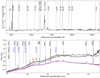 |
Fig. 2. MUSE (top panel) and MIRI MRS (bottom panel) integrated spectra for NGC 424 extracted from the same region, i.e. the MIRI MRS Ch 1 (orange square in Fig. 1). All the emission lines detected in each spectrum are highlighted. Warm molecular hydrogen transitions in the MIRI MRS spectrum are shown in blue. Black and purple spectra in the bottom panel represent the integrated MRS spectrum extracted from the entire FoV and from the 1 arcsec2 nuclear region of NGC 424, respectively. Red labels mark the positions of PAHs features at 11.25 and 12 μm. Grey spectrum in the bottom panel is the Spitzer IRS high-resolution extracted in full mode normalised to the MIRI MRS integrated spectrum. |
MIR emission line fluxes from MIRI/MRS channels, in units of MegaJansky/steradians.
3.1. JWST/MIRI MRS emission line fitting
To extract the highly ionised and warm molecular gas properties from MRS data, we performed a preliminary Voronoi tessellation (Cappellari & Copin 2003) in order to achieve an average signal-to-noise ratio (S/N) of 20 per wavelength channel on the continuum around emission lines of interest. In this work we focus on three emission lines tracing the ionised and warm molecular phases. In particular, we considered the [Ne V]14.3 μm (ionisation potential (IP) of 97 eV), [Ne III]15.5 μm (IP = 41 eV), and H2S(1) 17 μm (hereafter [Ne V], [Ne III], and H2S(1), respectively) emission lines from Channel 3 (Ch3, hereafter) MEDIUM and LONG, respectively. The choice of these specific emission lines is justified as they are among the strongest emission lines for each category (i.e. high- and low-ionisation potential transitions and molecular H2), and have many further advantages. First, these transitions occur in the same channel and thus are characterised by the same pixel scale (i.e. 0.2″/pixel) and a similar spatial resolution (see Appendix A). Second, since the attenuation curve at these wavelengths is almost flat, we expect a similar and mild attenuation of the line fluxes (Lai et al. 2024; Donnan et al. 2024), making the flux-derived properties reliable. The emission line fitting analysis of the mentioned transitions was performed on the PSF-subtracted Ch3 data cube due to the outshining emission from the unresolved nucleus. As a consequence, to investigate the spatial features of both the narrow and broad components of emission lines we subtracted the model PSF in each spectral channel following the routine described in Appendix A.
We performed a local continuum subtraction, focusing on two independent spectral regions encompassing a velocity range of ±2500 km s−1 around each emission line (for a similar approach to MIRI MRS data see Bajaj et al. 2024). In particular, we used the Penalized Pixel-Fitting (pPXF, Cappellari & Emsellem 2004) code on the previously binned spaxels to fit a first degree polynomial to the continuum underlying the emission line. Moreover, we simultaneously fit the emission line in the selected wavelength range, with one or two Gaussian components, to properly fit the continuum shape. Then, we subtracted the best-fit continuum and obtained a continuum-subtracted model cube that we spatially smoothed with a Gaussian kernel with a σ = 1 spaxel (i.e. 0.2″). The spatial smoothing does not affect the MRS spatial resolution at this wavelength, since in Ch3 the pixel size is smaller than the PSF (see also Appendix A).
We then analysed the smoothed continuum-subtracted data cube to perform a detailed emission line fitting. In particular, we independently fitted the [Ne V], [Ne III], and H2S(1) emission lines with a different number of Gaussians. Due to line asymmetries of the [Ne V], [Ne III] ionised transitions, two Gaussians were necessary to reproduce the line profile. On the other hand, the H2S(1) was well reproduced using a single Gaussian component. We used the MPFIT fitting tool (Markwardt 2009) to fit the emission lines in each spaxel. To decide the optimal minimum number of Gaussian components necessary to reproduce the line profile we applied a reduced χ2 selection and a Kolmogorov-Smirnoff test on the residuals of to the best fits in each spaxel, using a fiducial p value of 0.8 (for more details on the fitting algorithm see Marasco et al. 2020).
As a result of the multi-Gaussian fit, we obtained a dedicated model cube for each Gaussian component and one for their total best-fit profile. In particular, we considered the Gaussian component with lower width to be representative of the systemic disc kinematics and the broader component to trace the outflowing gas. Figure 3 shows the integrated spectra extracted from a circular aperture with radius of 0.6″ located in the redshifted side of the galactic disc. Top panels in Fig. 3 show the multi-Gaussian best-fit model used to reproduce the [Ne III] and H2S(1) line profiles. We observe that the narrower component of the [Ne III] line profile follows similar kinematics as the H2S(1) line. On the other hand, a broader blueshifted component of the [Ne III] is detected at high-S/N over the entire Ch3 FoV. The [Ne V] shows a line profile similar to that of [Ne III] but with a broader and more prominent component that we associate with an AGN-driven wind, possibly due to its higher ionisation potential (see Sect. 4.4 for a detailed discussion). Being more sensitive to the intense AGN radiation field in the circumnuclear region, the [Ne V] transition is well suited to trace the properties of such a hypothetical wind.
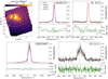 |
Fig. 3. Multi-phase Gaussian fit of the [Ne III], H2S(1), [O III]λ5007, and CO (2-1) emission lines from MIRI/MRS, MUSE, and ALMA data cubes, respectively. Top left panel: [Ne III] emission tracing the redshifted ionised gas, obtained collapsing the flux in the spectral window 15.56–15.57 μm rest-frame from the PSF subtracted data cube (see Appendix A). White contours represent arbitrary [OIII] flux levels from MUSE data. North is up and east is left. Top right panels: Integrated [Ne III] and H2S(1) emission extracted from the black circular aperture of radius 0.6″, shown on the left panel. Bottom left: Integrated [O III]λ5007 emission and best-fit extracted from the same aperture shown in the top left panel. Bottom right: Integrated CO (2-1) emission extracted from spaxels with S/N ≥ 3, covering the nuclear region of NGC 424, as is shown in the bottom panel of Fig. 4. Data and total best-fit model are in black and red, respectively. The sum of the single Gaussian best-fit components is shown in blue (narrow), and orange (broad). Bottom panels show the residuals in green. Vertical dashed grey lines mark the rest-frame wavelength of the transitions. Data and best-fit are normalised to the peak of the observed spectrum. |
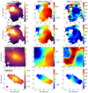 |
Fig. 4. From top to bottom: NGC 424 disc emission traced by [Ne III], H2S(1), [OIII], and CO (2-1) emission lines. The disc emission is traced by the total line profile of the H2S(1) and CO (2-1) transitions and by the narrower Gaussian component for the [Ne III] and [O III] emission lines. From left to right we show the emission line integrated flux, line of sight (LOS) velocity and velocity dispersion maps corrected for instrumental broadening. The integrated logarithmic flux maps are in unit of MJy/sr, 10−20 erg/s/cm−2, and Jy/beam for MIRI, MUSE, and ALMA maps, respectively. The green and grey circles are the MIRI and MUSE PSF, respectively. The ALMA beam is represented as a magenta oval. From top to bottom, a S/N mask of 3, 3, 5, and 3 was applied to moment maps. MIRI moment maps are obtained from the emission line fitting of the point-source subtracted data cube. North is up and east is left. |
3.2. MUSE emission line fitting
The routine used to perform the spatially resolved ionised gas analysis from the MUSE data cube was the same as the one used for the MRS data, discussed in Sect. 3.1, and tailored to MUSE (for an application of this routine to MUSE data see Venturi et al. 2018; Mingozzi et al. 2019; Marasco et al. 2020; Marconcini et al. 2023; Ulivi et al. 2024). In particular, we performed the Voronoi tessellation requiring an average S/N per wavelength channel of 100 on the continuum between 5150 Å and 8900 Å, masking the emission lines within this spectral window. We performed the continuum fitting spanning approximately the entire range of the MUSE spectral coverage, i.e. 4750–9000 Å, which is optimal as it includes many stellar absorption features. The stellar continuum fit was performed with the pPXF tool, using a linear combination of synthetic single stellar population (SSP) templates from Vazdekis et al. (2010). The templates were convolved with the MUSE spectral resolution, then shifted, broadened, and combined with a first-degree additive polynomial to reproduce the observed features. To account for possible absorptions underlying Balmer emission lines, we fitted the SSP templates together with the main gas emission lines, i.e. Hα, Hβ, [OIII]λλ4959,5007,[NII]λλ6549,6584, [SII]6716,6731. We then subtracted the best-fit continuum in each bin and obtained a continuum-subtracted model cube.
Similarly to the method described in Sect. 3.1, we fitted the mentioned emission lines in the continuum-subtracted cube with up to two Gaussian components, tying the velocity and velocity dispersion of each component. Moreover, we fixed the flux ratio between the two lines in each doublet, i.e. [OIII]λλ4959,5007, and [NII]λλ6549,6584, as given by the Einstein coefficients of the two transitions (Osterbrock & Ferland 2006). The optimal number of Gaussian components is decided based on the χ2 minimisation and a Kolmogorov-Smirnoff test, as was already described in Sect. 3.1. As a result, we obtained an emission-line model cube for all the mentioned transitions. The bottom left panel in Fig. 3 shows the integrated spectrum and best-fit of the [O III]λ5007 emission line extracted from the circular aperture shown in Fig. 3. In the following, we focus on the brightest (and highest ionisation, in the optical) emission line, i.e. [O III]λ5007 the transition (hereafter [OIII]) to trace the ionised gas features from the MUSE data.
3.3. ALMA emission line fitting
To analyse the properties of the cold molecular gas in NGC 424, we exploited the CO (2-1) transition observed in the ALMA band 6 data. Since the continuum was already subtracted in the uv plane during the data reduction we perform a single-Gaussian fit to the line profile. As for the H2S(1) transition, a single Gaussian was sufficient to reproduce the line profile in each spaxel based on the χ2 and the Kolmogorov-Smirnoff test. Bottom right panel in Fig. 3 shows the integrated CO (2-1) spectrum and best-fit extracted from a circular region of a 2″ radius, centred on the nucleus, and considering all spaxels with S/N ≥ 3 (i.e. from the region shown at the bottom panel in Fig. 4).
4. Results
In this section, we trace the ionised and molecular gas properties exploiting multi-band data from MIRI, MUSE and ALMA (see Sect. 2). We explored the molecular and ionised gas content within NGC 424, from the circumnuclear scale up to ∼5 kpc, providing a comprehensive analysis of the gas properties across different phases. In particular, we used the H2S(1) and CO (2-1) transitions to study the molecular gas component of the disc, from pc scales up to ∼1 kpc (see Sects. 4.1–4.7). Due to its intermediate ionisation potential and high S/N, and considering that the dust attenuation in the MIR regime is orders of magnitude smaller than in the optical regime (Gordon et al. 2023), the [Ne III] emission line is an optimal tracer of the ionised gas component within the dust-enshrouded inner disc. On the other hand, due to its higher ionisation potential and the circumnuclear scales covered by the MIRI MRS observations, the [Ne V] is expected to trace gas that is highly ionised by the AGN radiation field. Finally, exploiting the multi-Gaussian fit of the [OIII] and [Ne III] emission lines described in Sects. 3.2–3.1 and shown in Fig. 3 we were able to disentangle the ionised gas component within the disc and the broader blueshifted component, possibly associated with an AGN-driven wind.
4.1. Multi-phase 3D disc kinematic model
As a result of the multi-Gaussian fit described in Sect. 3, we obtained an emission-line model cube that is representative of the disc component in NGC 424 by isolating the narrower Gaussian component used to reproduce the line profile in each spaxel. Figure 4 shows the disc component traced by the ionised, warm molecular, and cold molecular emission, obtained from the MUSE, MIRI, and ALMA data cubes, respectively. Overall, the moment maps in Fig. 4 show that the morphology of the rotating disc probed by different gas phases is consistent across all tracers. We performed a detailed 3D kinematic modelling of the disc features to explore possible differences in the disc kinematics, infer the galaxy dynamical mass and explore the co-existence of multiple gas phases in the gaseous disc.
To model the multi-phase disc properties, we used our tool MOKA3D (Modelling Outflows and Kinematics of AGN in 3D), presented in Marconcini et al. (2023) and tailored to fit the multi-phase gas kinematic and geometry exploiting 3D data cubes. We modelled the disc properties of the warm and cold molecular, and ionised gas phases using the disc component traced by the H2S(1), CO (2-1), [Ne III], and [O III], respectively4. For each gas phase we adopted a thin-disc geometry with a height smaller than the spatial PSF. The thin-disc geometry is supported by the absence of significant bulge or bar components that could increase the height of the disc. Moreover, observations and models consistently find typical disc height-to-radius ratios of the order of 10−2, validating the thin-disc assumption (van der Kruit & Searle 1981; Nakanishi & Sofue 2006; Patra 2020; Ghosh & Jog 2022). Finally, considering the FWHM of the MUSE PSF of 0.8–1″ (i.e. 220 pc at the source distance), implies that any vertical disc structure, whose scale height is of the same order or smaller, cannot be spatially resolved in our data. We divided the disc in a different number of concentric circular shells. The number of shells used in the modelling is reported in Table 2 and is determined by the data spatial resolution and the maximum extent of the disc covered by the available FoV. For each observation we first set the outer radius of the disc and then set the width of each shell to be equal to the FWHM of the PSF. This approach ensures that the spatial sampling of the model matches the resolution limit of the data, maximising the use of the available spatial resolution (for details on the MOKA3D multi-shell set up see Marconcini et al. 2025). Therefore, the number of shells used to fit the observed disc properties in different gas phases in the final model depends on the instrument tracing a specific gas phase. In each shell, we independently fitted a single free parameter, i.e. the disc circular velocity (Vrot), while keeping the intrinsic velocity dispersion of the model clouds and the disc inclination with respect to the line of sight (β) fixed. These assumptions are commonly adopted in kinematic modelling to mitigate degeneracies between the rotating velocity, velocity dispersion, and inclination (e.g. Förster Schreiber et al. 2006; Epinat et al. 2010; Förster Schreiber et al. 2018), especially since we observe no kinematically disturbed motions as warps from the gas kinematic maps. To reduce the number of free parameters and thus reduce the degeneracies affecting the fit, the centre of the disc and the position angle are not fitted with MOKA3D but are measured with a separate routine. In particular, to infer the centre of the disc model we collapsed the narrow component used to fit the line profile of each tracer and performed a 2D Gaussian fit to the collapsed image. Then we fixed the position angle tracing the disc minor axis from the measured centre. The fitting procedure can be summarised as follows. We initially fitted a single-shell model to the entire disc to derive global best-fit estimates of the circular velocity, disc inclination, and intrinsic velocity dispersion. Assuming that the derived inclination and velocity dispersion are constant across the disc, we then fixed these parameters and performed a multi-shell fit leaving the circular velocity free to vary with radius, and obtaining the rotation curve shown in Fig. 5. For completeness, we also checked that our measured value for the disc position angle from MUSE data is consistent with the values estimated with the PaFit Python package (Krajnović et al. 2006), tailored to measure the global kinematic position angle from the stellar kinematic in integral field data. The free and fixed best-fit parameters obtained for the disc fit of all the gas components using MOKA3D are listed in Table 2. The comparison between the observed and modelled moment maps with MOKA3D is described in Appendix C.
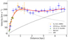 |
Fig. 5. NGC 424 rotation curve inferred with MOKA3D using the H2S(1) (orange) and CO (2-1) (green) emission, and the narrow component of the [O III] (blue) emission line, from MIRI/MRS, ALMA, and MUSE, respectively. The rotation curve obtained fitting the narrow component of the [Ne III] shown in Fig. 4 is not reported, as the trend is similar to the H2S(1). The dotted black and grey curves represent the best-fit velocity profile of the DM (Eq. (3)) and baryonic matter (Eq. (2)), respectively. The total best-fit profile is shown as a solid red curve. The averaged rotating velocity and inclination values are listed in Table 2. Details on the MOKA3D disc model are discussed in Sect. 4.1. |
Figure 5 shows the disc rotation curve inferred with MOKA3D fitting the disc component in MIRI, ALMA, and MUSE data. Interestingly, we observe that the disc velocity traced by different instruments is consistent at any distance up to the maximum FoV covered by each instrument. The gas circular velocity in the circumnuclear region traced by MIRI and ALMA has a low intrinsic and projected velocity, which slowly increases moving to larger distances, as traced by the fit of the MUSE data. The rotation curve shown in Fig. 5 is consistent with the expected profile for a simple gas disc in a galaxy, with no warps or distortions induced by a galactic bar.
4.2. Rotation curve fitting and dynamical mass
From the inferred best-fit intrinsic rotating velocity profile in Fig. 5, we could estimate the dynamical mass of NGC 424 within the maximum radius covered by MUSE data. In particular, we assumed that the gas is distributed in a thin disc, and that the stellar mass is distributed as the gas component with the gas mass surface density, Σ(r), distributed as the surface brightness, and described as I(r)=I0 × e( − r/RD), with I0 representing a normalisation constant. Under these assumptions, Freeman (1970) showed that the circular velocity can be expressed as
 (1)
(1)
where I and K are the modified Bessel functions computed at r = 2RD. Σ0 is a mass distribution constant used to normalise the gas and stellar contribution, and RD is the galaxy scale radius. The integrated mass surface density across all radii (Mdyn) can be expressed as Mdyn = 2πRD2Σ0. Inserting the definition of Mdyn in Eq. (1), we obtained
 (2)
(2)
Additionally, since the observed rotation curve flattens after ∼1.5 kpc, we included the dark matter (DM) contribution to the rotation curve by assuming a Navarro-Frenk-White (NFW) profile (Navarro et al. 1996, 1997), described as
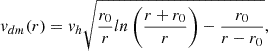 (3)
(3)
where vh = (4πr02ρ0 G)1/2 is the DM characteristic velocity, and ρ0 and r0 are the characteristic density and scale length of the DM profile, respectively. For the sake of simplicity, we followed the Lin & Li (2019) prescription and fitted vh instead of ρ0. Therefore, including the DM contribution to the observed rotation curve, we can write the total rotation velocity profile as
 (4)
(4)
where v(r) and vdm are defined in Eqs. (2)–(3).
Since we measured the intrinsic, de-projected multi-phase circular velocity profile using MIRI, MUSE, and ALMA data, covering scales from 20 pc with ALMA, up to 5 kpc with MUSE, we can fit Eq. (4) to the rotation curve shown in Fig. 5. Unfortunately, since our observations cover a maximum de-projected scale of ∼5 kpc from the nucleus we cannot properly constrain simultaneously the DM characteristic density and length, which are expected to contribute significantly at larger scales. Therefore, we assumed a characteristic scale length of r0 = 8.1 ± 0.7 kpc as recently found by Lin & Li (2019) for the Milky Way and fit the dynamical mass (Mdyn), the baryonic mass scale radius (RD) and the DM characteristic velocity, vh. As a result of the fit, we obtained the dashed red curve shown in Fig. 5, which corresponds to the best-fit parameters Mdyn = 1.09 ± 0.08 × 10¹⁰ M⊙, RD = 0.48± 0.02 kpc, and vh = 593 ± 35 km s−1. Uncertainties on the derived parameters are evaluated at the 16th and 84th percentiles. The best-fit rotation curve, including the contribution from baryonic mass and DM, accurately reproduces the intrinsic circular velocity profile inferred with MOKA3D. In particular, we observe that the DM contribution starts to be significant at radii larger than ∼2 kpc and that the NFW profile is well suited for reproducing the observed rotation curve.
4.3. 3D ionised outflow kinematic modelling
We used the [O III] and [Ne III] emission lines, from MUSE and MIRI/MRS IFS data, to explore the ionised gas properties in the optical and MIR, respectively. As is discussed in Sects. 3.1 and 3.2, we used up to two Gaussian components to fit each observed emission line profile. Using a tailored number of Gaussian components to fit the observed emission line profiles is a well-tested method that has proven to be efficient in separating the emission originating from the rotating disc – typically observed as a narrow, symmetric component – and the emission from outflowing gas – observed as an asymmetric, broader component – (Venturi et al. 2018; Mingozzi et al. 2019). In this section we discuss the ionised outflow properties as a result of the separation of symmetric (narrow) and asymmetric (broad) components used to reproduce the observed line profiles of the [O III] and [Ne III] emission lines on a spaxel-by-spaxel basis.
To infer the ionised outflow properties observed both in [O III] and [Ne III] emission lines, we again used our MOKA3D kinematic model, which has proven to be particularly efficient in modelling outflow features at an unprecedented level of detail using IFS data from various instruments (Marconcini et al. 2023; Cresci et al. 2023; Ulivi et al. 2025; Perna et al. 2025; Marconcini et al. 2025; Ceci et al. 2025). In particular, we separately modelled the outflow properties traced by the broad components of the [O III] and [Ne III] line profiles and finally discussed how the ionised outflow phase morphology and kinematics vary as a function of wavelength.
To model the outflow properties, we adopted a bi-conical-shaped outflow with a constant radial velocity field originating from the unresolved nucleus. To test the scenario of a tight interplay between the outflow and the elongated enhanced velocity dispersion region shown in Fig. 4 that will be described in Sect. 4.6, we assumed the cone axis to be directed along the galaxy major axis, i.e. we fixed the outflow position angle to 118°5.
For the MUSE data, since the observed outflowing gas clouds extend up to 5″ in projection (i.e. 1.2 kpc) and we detected extended blueshifted emission towards the east direction, (see bottom panels in Fig. 6) we assumed a large outer opening angle of 70°. A wide outer opening angle is necessary to simultaneously reproduce such an extended blueshifted outflow features on such a compact scale. Similarly, towards the west direction, we observe a more collimated redshifted wind that is probably obscured by the galactic disc and represents the counterpart of the blueshifted wind on the east side. Therefore, to model the observed features traced by the [O III] emission line we adopted a bi-conical geometry.
 |
Fig. 6. MOKA3D best-fit model for the ionised outflow traced by the broad component of the [O III] from MUSE data. Top panels: 3D reconstruction of the ionised gas clouds colour-coded based on their position with respect to the plane of the sky and observed along the outflow axis (left, i.e. as if the conical outflow axis coincide with the line of sight of the observed) and along the line of sight (right). The XY represents the plane of the sky, while the Z is the LOS. The dotted black lines in the right panel show the bi-conical outflow axis direction. According to the colourbar, blue and red clouds are blueshifted and redshifted, respectively. The bubble size is representative of the intrinsic cloud flux. Bottom panels: Data (top), MOKA3D best-fit (middle) and residual (bottom) moment maps, i.e. the integrated flux, the LOS velocity, and velocity dispersion maps. The residual maps are obtained by subtracting the model from the observed moment maps. Maps are masked at a S/N of 3. North is up and east is left. |
The free parameters of the model are the outflow inclination, the intrinsic radial velocity, velocity dispersion, and the inner opening angle of the cone. As a result of the MOKA3D fit, we obtained an inclination of the cone axis with respect to the plane of the sky of β = 35° ± 3°, an outflow radial velocity of Vout = 990 ± 35 km s−1, an intrinsic outflow velocity dispersion of Vdisp = 95 ± 25 km s−1, and inner opening angle of 20° ± 7° (see also Table 3).
Best-fit parameters for the ionised outflow properties in NGC 424, traced by [Ne III] and [O III]λ5007 emission lines and inferred with the MOKA3D framework.
Based on the best-fit outflow parameters and taking into account the disc inclination (see Sect. 4.1 and Table 2), we remark that the outflow is directly impacting on the gaseous disc, having the outflow and disc a similar inclination with respect to the line of sight. Moreover, based on the MOKA3D best-fit the outflow has an inner cavity surrounding its axis, which can be ascribed to the fact that it cannot propagate freely while interacting with the disc, due to the high-resistance path and column density.
To infer the outflow properties traced by the MIR [Ne III] emission line, we followed a similar approach as for the [O III] emission line. We considered the broad Gaussian component of the [Ne III] line profile in each spaxel and created the moment maps shown in Fig. 7, which due to the low S/N of the broad component of the [Ne III] trace only the west direction. Interestingly, since [Ne III] traces emission at longer wavelengths with respect to the [O III] emission line and is thus less obscured by the galactic disc, we detect the SW cone, i.e. the receding cone at much higher S/N.
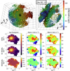 |
Fig. 7. Same as in Fig. 6 for the [Ne III] emission line from MIRI MRS Ch3. Maps are masked at a S/N of 2. |
To model the [Ne III] outflow we assumed a conical-shaped wind morphology with the same inner and outer opening angle and position angle as for the [O III]-traced outflow. Using MOKA3D to reconstruct the outflow morphology and kinematics we estimated an outflow inclination for the west side of β = 25 ° ±7° with respect to the plane of the sky, an outflow radial velocity of Vout = 975 ± 30 km s−1, an intrinsic outflow velocity dispersion of Vdisp = 90 ± 10 km s−1, consistently with the [O III] estimates (see Table 3). Interestingly, as reported in Table 3, we found consistent estimates for the [O III] and [Ne III] outflow intrinsic kinematic and inclination, highlighting the pivotal role of a sophisticated kinematic model as MOKA3D to account for the complex outflow features.
4.4. Highly ionised outflow
The highest-S/N highly ionised emission line in our MIRI/MRS data is the [Ne V] that falls in the Ch3 MEDIUM band. Unfortunately, the S/N on the broad component of the [Ne V] emission line is not sufficient to provide a reliable constraint on the highly ionised wind morphology. Therefore, we integrated the emission-line profile of the [Ne V] over the entire FoV of Ch3 MEDIUM and performed a two Gaussian-component fit to the line profile, which presents the same blueshifted line wing as for the [Ne III] and [O III] line profile (see Fig. 8). As a result of the fit, we found a velocity dispersion for the broad component of 283 ± 17 km s−1 and a blueshift with respect to the rest-frame emission of 61 ± 5 km s−1. Assuming that the [Ne V]-traced outflow has the same morphology as the [O III]- and [Ne III]-traced outflows and that the outflow is propagating at constant radial velocity, we can correct the maximum observed [Ne V]-traced outflow velocity of 812 ± 47 km s−1for projection effects6. Indeed, assuming the same inclination of the [Ne III] outflow of 25° ± 7° (see Table 3) we found Vout, [Ne v] = 900 ± 50 km s−1. Such a value for the intrinsic outflow velocity inferred for the highly ionised phase is consistent with the values derived for the warm ionised phase listed in Table 3.
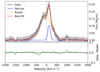 |
Fig. 8. Multi-Gaussian fit of the integrated [Ne V] emission line from the total MIRI/MRS Ch3 MEDIUM band. Data and total best-fit model are in black and red, respectively. The narrow and broad Gaussian components are shown as solid blue and orange lines, respectively. The bottom panel shows the residuals in green. The vertical dashed grey line marks the rest-frame wavelength of the [Ne V] transition. |
4.5. Ionised outflow energetics
To infer the energetic impact of the ionised outflow in NGC 424, we exploited the tomographic outflow reconstruction obtained with MOKA3D, which provides the distribution of ionised gas clouds within the outflow and the intrinsic (i.e. de-projected) outflow properties. In particular, similarly to the method used in Marconcini et al. (2023) and based on the model by Cano-Díaz et al. (2012), we computed the amount of ionised mass traced by the [Ne III] emission lines in each spaxel using the relation
![Mathematical equation: $$ \begin{aligned} M_{\rm out} = 5.33 \times 10^7 \left( \frac{L_\text{[OIII]}}{10^{44} \, \text{ erg} \, \text{ s}^{-1}} \right) \left( \frac{n_{\rm e}}{1000 \, \text{ cm}^{-3}} \right)^{-1} \ \ M_\odot ,\end{aligned} $$](/articles/aa/full_html/2025/09/aa54797-25/aa54797-25-eq5.gif) (5)
(5)
where L[OIII] is the luminosity of the broad component of the [O III] emission line corrected for dust attenuation (see Appendix B), ne is the average electron density of the ionised gas. Therefore, using Eq. (5) we can convert the flux density of the ionised wind in mass. Assuming the flux density within each spaxel to be constant over time and the outflow to subtend a solid angle, Ω, we can use Eq. (5) to compute the mass outflow rate (Ṁout), i.e. the amount of ionised mass crossing a distance, R, with velocity Vout, as
 (6)
(6)
Finally, we calculated the kinetic energy (Ekin), kinetic luminosity (Lkin) and momentum rate ( ) of the outflow as
 (7)
(7)
 (8)
(8)
 (9)
(9)
In order to be able to compare the outflow energetics traced by the [O III] and MIR emission lines, and due to the limited FoV of MIRI with respect to MUSE, in the following we refer to the [O III] luminosity extracted from the same region considered for the [Ne III] and [Ne V] emission lines, i.e. the MIRI Ch3 FoV.
For the ionised phase traced by the [O III] emission line, we found a total outflowing gas mass of Mout = 24 ± 11 × 104 M⊙using an average electron density of < ne > =570 ± 360 cm−3 obtained from the total line profile of the [SII]λλ6716,6731 doublet of MUSE data (see Appendix B and Fig. B.1). Using the best-fit values for the outflow velocity of Vout = 990 ± 35 km s−1 and the outflow de-projected size inferred from MIRI observations of 1.1 ± 0.1 kpc (assuming as uncertainty half the FWHM of the MUSE PSF), we estimated a mass outflow rate
of  ± 1.0 × 10⁻¹ M⊙ yr−1. As a comparison, we computed the outflowing gas mass and mass outflow rate from the broad component of the Hα recombination line assuming the same gas electron density and outflow velocity as for the [O III] analysis. After correcting for extinction, we found Mout = 90 ± 46 × 104 M⊙and
  ± 4.5 × 10⁻¹ M⊙ yr−1. Therefore, comparing the outflowing gas masses traced by [O III] and Hα we found Mout,[O III]/Mout,Hα = 0.26. This value is consistent with the typical ratio measured in Seyfert galaxies and such a discrepancy has to be ascribed to the different volume of 3D regions of [O III] and Hα emission (see also Carniani et al. 2015; Karouzos et al. 2016). Indeed, the volume of gas emitting the Hα recombination line is expected to be larger and more extended along the line of sight with respect to the [O III] line, thus tracing larger amount of ionised mass.
To infer the energetics of the ionised outflow traced by the MIR emission lines, such as the [Ne III] and [Ne V], we need to take into account the Neon emissivity as well as its abundance. A detailed description of the procedure to infer the amount of ionised mass traced by MIR emission line is presented in Ceci et al. (2025). Assuming a solar abundance of [Ne/H] of 7.93 (Asplund et al. 2009), a ionised gas temperature of Te = 104 K we can write the ionised mass traced by the Neon emission lines as
![Mathematical equation: $$ \begin{aligned} M_\text{ Neon} = \alpha (\gamma , [\mathrm{Ne/H}]) \, \left( \frac{L_\text{ Neon}}{10^{36} \, \text{ erg} \, \text{ s}^{-1}} \right) \left( \frac{n_{\rm e}}{200 \, \text{ cm}^{-3}} \right)^{-1} \, M_\odot ,\end{aligned} $$](/articles/aa/full_html/2025/09/aa54797-25/aa54797-25-eq13.gif) (10)
(10)
where α(γ,[Ne/H]) is a factor that depends on the emissivity of different transitions and on the solar abundance of the Neon atom7 (for a detailed discussion of the outflowing gas mass estimate see Cano-Díaz et al. 2012, Carniani et al. 2015, Ceci et al. 2025). In particular, we get α = 46 and α = 3, for the [Ne III] and [Ne V] emission lines, respectively.
Therefore, we estimated outflowing gas mass of M[Ne III] = 5.4 ± 2.7 × 10⁴ M⊙and M[Ne V] = 1.9 ± 0.9 × 10⁴ M⊙. Using Eq. (6) and the outflow kinematic properties listed in Table 3 we estimated a mass outflow rate of ![Mathematical equation: $ \dot M_{\mathrm{out}, [{\mathrm{Ne}{{ {\text{ III}}}}}]} $](/articles/aa/full_html/2025/09/aa54797-25/aa54797-25-eq14.gif) = 4.5 ± 2.3 × 10⁻² M⊙ yr−1, and
= 4.5 ± 2.3 × 10⁻² M⊙ yr−1, and ![Mathematical equation: $ \dot M_{\mathrm{out},[{\mathrm{Ne}{{ \small{\text{ V}}}}}]} $](/articles/aa/full_html/2025/09/aa54797-25/aa54797-25-eq15.gif) = 1.6 ± 0.8 × 10⁻² M⊙ yr−1.
= 1.6 ± 0.8 × 10⁻² M⊙ yr−1.
The results for the outflow energetics traced by the [Ne V], [Ne III], and [O III] emission lines are listed in Table 4. To estimate the ionised outflow energetic traced by the [O III] emission line, we corrected the line flux for the dust attenuation, using the resolved dust attenuation map shown in Fig. B.1 computed assuming a Calzetti et al. (2000) attenuation law (see also Appendix B). To correct the MIR emission line fluxes, we used the Gordon et al. (2023) attenuation curve, tailored to the MIR regime. In Table 4 we report the ratio between the outflow kinetic luminosity of the various tracers (also referred as the outflow kinetic power) and the AGN bolometric luminosity (Lbol = 1.4 × 1044 erg s−1 8). Overall, the estimates for the ionised outflowing gas mass as well as the mass outflow rate traced by the [O III] emission line are largely dominant with respect to the [Ne III] and [Ne V] estimates. In Sect. 5.2 we present a possible interpretation for this result as well as a comparison with estimates from the literature.
Summary of outflow energetic properties in NGC 424.
Overall, our analysis exploiting archival [O III] observations and recent MIRI/MRS observations revealed that in NCG 424 the largest contribution to the outflowing wind energetics is carried by the warm ionised gas traced by the [Ne III] and [O III] emission lines. To a lesser extent, the highly ionised gas traced by [Ne V] emission line reveals a mass outflow rate an order of magnitude smaller with respect to the warm-ionised phase.
4.6. Enhanced velocity dispersion along the galaxy minor axis
The narrow component velocity dispersion maps of [Ne III], CO (2-1), [O III], and to a lesser extent of H2S(1), show an elongated enhancement of gas velocity dispersion along the disc minor axis (see Fig. 4). Moreover, perpendicular to such an enhancement we observe deep minima of the gas velocity dispersion, especially in the ionised phase. Such features resemble the enhancement of gas velocity dispersion perpendicular to the outflow and radio jet direction in local Seyfert galaxies observed in previous works (e.g. González Delgado et al. 2002; Schnorr-Müller et al. 2014, 2016; Freitas et al. 2018; Finlez et al. 2018; Shimizu et al. 2019; Durré & Mould 2019; Shin et al. 2019; Feruglio et al. 2020; Venturi et al. 2021; Girdhar et al. 2022; Ulivi et al. 2024). The most credited scenario for this phenomenon suggests that such an enhancement is due to the impact of the radio jet onto the galaxy disc, perturbing the ambient gas in the ionised phase. Indeed, the observed extended velocity dispersion perpendicular to AGN jets and ionisation cones in sources with a low jet-disc inclination might result from a strong impact of the jet on the host material. Such a scenario is also consistent with cosmological simulations, showing that radio jets are capable of affecting and altering the host galaxy equilibrium (Weinberger et al. 2017; Pillepich et al. 2018) and with jet-ISM interaction hydrodynamic simulations (Mukherjee et al. 2016, 2018; Meenakshi et al. 2022).
Such a phenomenon is also observed in the H2 warm molecular (Riffel et al. 2014, 2015; Diniz et al. 2015) and CO (2-1) cold molecular components (Shimizu et al. 2019). Studies presenting these results have proposed different explanations for such a phenomenon, all of which invoke a tight interaction between the AGN, the radio jet, and the host galaxy, discarding the hypothesis of instrumental effects such as beam smearing as the cause.
All of the aforementioned works found the velocity dispersion to be enhanced perpendicularly to the host galaxy radio jets and ionisation cones. Unfortunately, there is only weak evidence of a radio jet in NGC 424. Indeed, Nagar et al. (1999) observed a slightly elongated E-W radio structure using a VLA 20 cm image, later on confirmed by Mundell et al. (2000) with higher-resolution VLA 3 cm observations. Due to the low sigma detection of such radio detections, the presence of a radio jet is still unconfirmed. Nevertheless, we investigated the presence of such a radio jet from VLA 8.49 GHz (X band) data9 and found no evidence of bright radio spots or E-W structures, therefore casting doubts on the presence of a radio jet in NGC 424.
In Sects. 3.2 and 3.1 and in Fig. 3 we showed the presence of broad blueshifted emission possibly associated with an AGN-driven wind, which we further confirmed in Sects. 4.3 and 4.4. In particular, in Sect. 4.3 we showed that such a wind is well fitted by a large opening-angle (bi)conical outflow propagating at velocities of ∼103 km s−1and interacting with the host galaxy due to the low inclination angle of the outflow axis with respect to the galaxy plane. Thanks to our detailed kinematical modelling of the AGN-driven wind, mainly traced by [Ne V] and [O III] emission, we strengthen the scenario of significant outflow-disc interaction possibly causing the observed enhancement of gas velocity dispersion along the minor axis, despite we have no evidences of a radio jet in NGC 424, which instead is a crucial ingredient in the scenario proposed by Venturi et al. (2021) and Ulivi et al. (2024).
An alternative scenario is discussed by Pilyugin et al. (2021) as such an elongated enhancement of the gas velocity dispersion along the galaxy minor axis has been observed also in a sample of MaNGA galaxies. The authors suggest that the presence of the region of enhanced gas velocity dispersion can be an indicator of a specific evolutionary path or evolution stage of the host galaxy. Moreover, they do not find evidence of such a region being related to the presence of an AGN and thus to a radio jet, but think it can rather be explained with a radial component of the gas velocity dispersion larger than the azimuthal and vertical components. Nevertheless, a complete understanding of the cause of this higher velocity dispersion in the radial direction is still missing.
4.7. Cold and warm molecular phases
We used the MIRI/MRS Ch3 LONG data cube and the ALMA band 6 high-resolution data cube to explore the warm and cold molecular gas phase properties, as traced by the H2S(1) and CO (2-1) transitions (see Sects. 3.1 and 3.3). To investigate possible non-circular motions in the cold molecular phase, we computed position-velocity diagrams (PVDs) along the major and minor axis of the galaxy, from a 0.8″ slit. As is shown in Fig. 9, the pure circular motions modelled with MOKA3D (see Fig. C.3 and Sect. 4.1) and shown in black contours, reproduce the observed features, with no evidence of outflowing gas along either the major or minor axis, as is also suggested by the residual maps shown in the bottom panel of Fig. C.3. Exploiting a PVD to infer the possible presence of outflowing material from ALMA data is a well-tested method that here confirms the pure rotating nature of the cold molecular phase in NGC 424 (Ramos Almeida et al. 2022; Audibert et al. 2023; Zanchettin et al. 2025). Moreover, Fig. 10 shows the velocity channel maps for the warm and cold molecular gas phases, traced by H2S(1) and CO (2-1) emission lines, respectively. As is suggested by the moment maps (Fig. 4) and line profiles (Fig. 3), the velocity channel maps confirm the absence of outflowing gas in the cold and warm molecular phases, as is suggested by the non-detection of emission in the high-velocity channels. A more quantitative assessment of the non-detection can be made by converting the RMS noise of the spectrum computed over the high-velocity regions of the line (e.g. here we computed it in both the blueshifted and redshifted 250–500 km s−1spectral region) into a molecular gas mass sensitivity. In particular, we extracted the spectrum from a circular region centred on the nucleus and with a radius equal to the ALMA FWHM (i.e. ∼0.45″). Then, assuming a CO (2-1) to CO (1-0) luminosity ratio of R21 = 0.7 (Leroy et al. 2009; Sandstrom et al. 2013), and a conservative CO-to-H2 conversion factor αCO = 4.3 M⊙ pc−2 (K km s−1)−1 (Bolatto et al. 2013), we estimate a 1 σ molecular gas mass upper limit of 3.3 × 10⁶ M⊙. As a comparison, this upper limit on the outflow mass is ≤10% of the total molecular gas mass of 3.2 × 10⁷ M⊙estimated from the same region. This fraction is consistent with findings in local galaxies, where the molecular outflow component is often found to be only a small fraction of the total molecular reservoir (Cicone et al. 2014; Fluetsch et al. 2019; Lamperti et al. 2022).
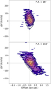 |
Fig. 9. Position-velocity diagrams extracted from a slit of width 0.8″ along the NGC 424 CO (2-1) kinematic minor axis (top panel, PA = 28°, see Table 2) and major axis (bottom panel, PA = 118°). CO (2-1) emission is masked at S/N ≤ 3. White contours correspond to arbitrary levels of the observed emission. Black contours correspond to arbitrary levels extracted from the best-fit model cube obtained with MOKA3D shown in Fig. C.3 and described in Sect. 4.1. |
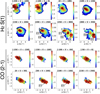 |
Fig. 10. Velocity channel maps at different velocity bins for the warm (H2S(1), top panels) and cold molecular (CO (2-1), bottom panels) gas components. Channel maps are in logarithmic scale and in units of MegaJansky/steradian (top panels) and Jansky/beam (bottom panel). Contours represent arbitrary flux level. Molecular gas knots in the galactic disc, discussed in Sect. 4.7, are labelled as C1, C2, and C3. North is up, east to the left. |
Interestingly, continuum-subtracted channel maps highlight the combination of diffuse and extremely clumpy structures along the disc major axis direction. In particular, flux maps in velocity intervals between [−200, 150] km s−1and [−150, 50] km s−1for the H2S(1) and CO (2-1) emission lines, respectively, appear smooth and diffuse. On the other hand, at projected velocities larger than 150 km s−1and 50 km s−1for the H2S(1) and CO (2-1) emission lines, respectively, we observe well-defined sub-structures, not observed in any of the ionised gas flux maps. Indeed, exploiting the MIRI/MRS spatial resolution after subtracting the PSF we noticed three resolved main clumps (C1, C2, C3) separated by a projected distance of 460 pc in the three most redshifted channel maps of the H2S(1) emission line shown in Fig. 10. Similarly, a clumpy structure is also detected at blueshifted velocities in the H2S(1) and CO (2-1) continuum-subtracted channel maps. Interestingly, the C1 clump detected in H2S(1) is also highlighted in the [50, 100] km s−1CO (2-1) channel map.
The co-spatiality of the same resolved clump (i.e. C1) both in H2S(1) and CO (2-1), observed at different projected velocities suggest a stratification of the molecular gas where the emission of the colder phase (i.e. CO (2-1)) originates from a more embedded region with respect to the warm phase (i.e. H2S(1)). The same conclusion is also supported by the lower circular velocity of the cold molecular phase as inferred from the kinematic fit in Sect. 4.1 (see also Table 2).
5. Discussion
5.1. Multi-phase elongated enhancement of the velocity dispersion
As is shown in Fig. 4, we found remarkable evidence of enhanced gas velocity dispersion along the galaxy minor axis both in the ionised and molecular phases, cold and warm, as traced by [Ne III], [O III], H2S(1), and CO (2-1) emission, respectively. Moreover, such an enhancement appears to be perpendicular to the ionised outflow detected both in [Ne III], [Ne V], and [O III] transitions. Thanks to a detailed modelling of the outflow properties (see Figs. C.4 and C.2, and Sect. 4.3) we discovered that the outflow is impacting the galactic disc and is reproduced well by a conical wind with an inner cavity along the axis.
To date, no previous works have detected such a phenomenon of enhanced velocity dispersion in the ionised, warm and molecular gas phases simultaneously. Moreover, despite previous AGN-focused observations and simulations ascribe the observed enhancement of velocity dispersion (see Sect. 4.6) to the radio jet impacting onto the host galaxy disc (Mukherjee et al. 2016; Venturi et al. 2018; Talbot et al. 2022; Audibert et al. 2023; Ulivi et al. 2024), we found the same pattern of velocity dispersion enhancement, with no evidence of a radio jet, consistently with the findings of Pilyugin et al. (2021). In the following section we present a detailed 3D morphological and kinematical analysis of the wind suggesting that the ionised outflow might play a crucial role in disturbing the ambient material and thus contributing to the observed enhancement of the gas velocity dispersion, despite the absence of a radio jet. Indeed, as listed in Table 4, we find that the Lkin/Lbol ratio for the total ionised phase (i.e. summing up the values obtained from the [O III]λ5007, [Ne V], and [Ne III] transitions) is ∼0.06%. Extrapolating the trend observed by Fiore et al. (2017) for the ionised phase, we find that such a ratio lies below the average trend, implying that the outflow in NGC 424 is likely not powerful enough to play a crucial role in quenching the SF or to expel large amounts of gas. Note that, including the contribution of the Hα emission line to the outflowing gas, we find a Lkin/Lbol ratio of 0.18%, which is consistent with the observed trend of ionised winds in the sample analysed by Fiore et al. (2017). Therefore, the ionised wind in NGC 424 may still play a role in compressing the ambient material and thus possibly causing the observed enhanced of the gas velocity dispersion. Finally, despite we do not find evidence of outflowing molecular gas both in the cold and warm phases, the CO (2-1) emission clearly shows enhanced velocity dispersion along the galaxy minor axis (see Fig. 4), suggesting that the ionised wind is sufficient to inject enough energy to disturb the ordered gas motion within the host galaxy disc. On the other hand, the warm molecular phase traced by the H2S(1) emission, only shows a marginal enhancement of the gas velocity dispersion along the disc minor axis and with a clumpier distribution than in other gas phases. Moreover, the peaks of the H2S(1) velocity dispersion lie mostly towards the edges of the FoV where the S/N is lower, thus preventing us to confirm a minor axis increase in the warm molecular phase.
5.2. Multi-phase outflow
Exploiting the multi-band observations of NGC 424 we observed a clear emission line asymmetry in warm and intermediate-to-high ionisation transitions such as the [Ne III], [O III], and [Ne V] emission lines from recent MIRI observations and archival MUSE data. On the other hand, the line profile of the cold and warm molecular transitions (i.e. CO (2-1) and H2S(1) ) considered in this work is always reproduced well with a single Gaussian profile, suggesting that such transitions originate from ordered motions within the gaseous disc, with no evidence of molecular gas outflows. The detailed morphological and kinematical modelling of the warm ionised outflow presented in Sect. 4.3 allowed for the investigation of the redshifted part of the AGN outflow in NGC 424, leveraging the infrared wavelength to optical transitions. The outflow partially lies behind the galactic disc, a positioning that makes it more attenuated in the optical regime.
We also investigated the highly ionised counterpart of the outflow by fitting the spatially integrated [Ne V] emission line (IP = 97 eV). Unfortunately, due to the low S/N of the broad component of this transition, we could not provide a detailed kinematical modelling as done for the [Ne III] and [O III] transitions. Nevertheless, we estimate an outflow velocity of the highly ionised phase traced by the [Ne V] emission consistent with the warm ionised components (see Sect. 4.4 and Table 3).
Our findings on the warm and highly ionised outflow rates traced by the [O III], Hα, [Ne III], and [Ne V] emission lines and presented in Sect. 4.5 suggest that the largest contribution to the mass outflow rate in NGC 424 has to be ascribed to the warm-ionised phase, as was also confirmed by recent JWST MIRI observations of local AGNs targeting the [Ne V] emission line (Zhang et al. 2024). Indeed, the mass outflow rate of the highly ionised phase traced by the [Ne V] emission line is about an order of magnitude smaller (see Table 4). Overall, our estimates for the mass outflow rate of the ionised phase are consistent with recent works studying the ionised outflow energetics in local Seyfert galaxies, showing mass outflow rates spanning the interval of Ṁout ∼ 10−2 ± 0.8 M⊙ yr−1 (e.g. Davies et al. 2020; Riffel et al. 2023; Zhang et al. 2024; Esposito et al. 2024). Nevertheless, our estimate of the mass outflow rate in NGC 424 is ∼ two orders of magnitude smaller with respect to the value reported for the same target by Kakkad et al. (2022). Indeed, studying the spatially resolved [O III] properties they found a mass outflow rate of  M⊙ yr−1. On the other hand, they also provided mass outflow rate estimates computed from the integrated 3″ fibre spectra and 1.5″ × 10″ integrated slit spectra, of 0.1 and 0.05 M⊙ yr−1, respectively. We notice that our results are consistent with those presented in the integrated analysis of Kakkad et al. (2022) but not with the resolved estimates. The discrepancy between our resolved estimate and that presented in Kakkad et al. (2022) could be due to the amount of line flux associated to the outflow and its extension. Indeed, as is shown in Fig. A4 in Kakkad et al. (2022), they found outflowing gas up to extremely large scales (4.5 kpc) compared to our analysis (1.6 kpc), therefore summing up fluxes from a larger number of pixels. This is also supported by the fact that both estimates are consistent when considering the values computed from the inner region of 3″. Moreover, at variance with Kakkad et al. (2022), we computed the [O III] ionised mass outflow rate only considering the emission from spaxels within the MIRI Ch3 FoV, in order to provide consistent results with the MIR analysis, and therefore neglecting part of the emission originating from the NE side of the nucleus. Finally, as presented in Sect. 4.5, we also estimated the amount of ionised mass from Hα emission. This value is ∼4 times larger than the ionised mass traced by the [O III] emission line and still 1.5 dex smaller with respect to the value provided in Kakkad et al. (2022). As is discussed in Carniani et al. (2015), the ionised mass traced by the [O III] emission line has to be considered as a lower limit of the total ionised mass when compared to the mass traced by recombination lines as Hα or Hβ (Karouzos et al. 2016; Rakshit & Woo 2018).
6. Conclusions
In this work we have presented the first observations of the MIRACLE programme, aimed at tracing the MIR radiation exploiting MIRI/MRS observations of the circumnuclear region of local AGNs in the 5–28 μm wavelength range. We completed the multi-phase analysis of the NGC 424 galaxy aided by archival MUSE and ALMA data, tracing the warm ionised and cold molecular phases. The main conclusions from this work are the following:
-
We traced the ionised ([Ne III], [O III]), warm (H2S(1)), and cold (CO (2-1)) molecular gas phases in the galaxy disc, revealing the intrinsic rotation curve from a few parsecs up to ∼5 kpc scales and providing an accurate estimate of the dynamical mass of the NGC 424 galaxy of Mdyn = 1.09 ± 0.08 × 10¹⁰ M⊙.
-
We present the first evidence of an elongated high–velocity–dispersion structure (σ ≥ 350 km s−1), oriented perpendicular to the ionisation-cone outflow, which is detected in the ionised, cold gas phase and marginally in the warm molecular gas phase. At variance with previous works, we mainly ascribe such a scenario to a tight interplay between the gaseous disc and the outflow – possibly due to the impact of wind on the host – causing highly turbulent gas in the perpendicular direction, without necessarily having a low-inclination radio jet.
-
We spatially resolved and modelled the ionised gas phase in the outflow traced by the broad component of the [Ne III] and [O III] emission lines, from MIRI and MUSE IFS data, respectively. We estimated outflow velocities of up to 103 km s−1 from both tracers and mass outflow rates of the order of 10−1.0 ± 0.4 M⊙ yr−1. Moreover, the 3D morphological and kinematical modelling supports the scenario of a tight interaction between the ionised outflow and the gaseous galactic disc, suggesting that the impact of the outflow on the disc might be as relevant as the impact of the jet in producing the observed enhancement of the velocity dispersion perpendicular to wind direction.
-
We fitted the spatially integrated [Ne V] emission line tracing the highly ionised outflow in NGC 424 and found an average wind velocity consistent with the warm ionised phase and a mass outflow rate of the highly ionised phase of 1.6 × 10⁻² M⊙ yr−1.
In conclusion, in this work we have exploited MRS data and archival MUSE and ALMA data to shed light on the physical properties of the NGC 424 active galaxy across various phases and scales. In particular, we have carried out a detailed analysis of the ionised outflow properties traced by MIR and optical emission lines, evaluating the energetic impact of the wind onto the host galaxy. Finally, with this work we have remarked on the necessity of carrying out a multi-wavelength analysis of AGN outflows, aided by optical, millimetre, and MIR observations to unveil the total energetics of outflows.
We estimated the redshift fitting the H and [O III]λλ4959,5007 emission lines from the integrated spectrum of MUSE data extracted from a circular region of 1″ centred on the nucleus.
The continuum was subtracted using the line free spectral channels in the spectral windows [226.91, 228.79] GHz and [229.29, 231.27] GHz.
For the disc component, we refer to the total line profile of the H2S(1) and CO (2-1) emission lines and to the narrower Gaussian component for the [Ne III] and [O III] emission lines.
The position angle is measured clockwise from North.
This value is estimated from the maximum value between the first and 99-th percentile of the line profile. This method to estimate the intrinsic outflow velocity has been deeply discussed in Marconcini et al. (2023).
Using Pyneb (Luridiana et al. 2012, 2015) and a gas electron density of 570 ± 360 cm−3 we computed a lines emissivity of γ[Ne III] = 1.25 × 10⁻²¹ erg s cm−3 and γ[Ne V] = 1.93 × 10⁻²⁰ erg s cm−3 for the [Ne III] and [Ne V] emission lines, respectively.
The AGN bolometric luminosity is estimated from the intrinsic Swift-BAT hard X-ray luminosity (14–195 KeV) (Kakkad et al. 2022).
These VLA data are the same data presented in Mundell et al. (2000), re-analysed in 2009 and downloaded from the NRAO archive https://www.vla.nrao.edu/astro/nvas/avla.shtml
Acknowledgments
CM, GC, AM, FM, FB, EB, GV and AF acknowledge the support of the INAF Large Grant 2022 “The metal circle: a new sharp view of the baryon cycle up to Cosmic Dawn with the latest generation IFU facilities”. CM, GC, AM, GT, FM, FB, EB also acknowledge the support of the grant PRIN-MUR 2020ACSP5K_002 financed by European Union – Next Generation EU. EDT is supported by the European Research Council (ERC) under grant agreement no. 101040751. AM, FM, GC, IL acknowledge support from project PRIN-MUR project “PROMETEUS” financed by the European Union – Next Generation EU, Mission 4 Component 1 CUP B53D23004750006. AM acknowledges INAF funding through the “Ricerca Fondamentale 2023” programme (mini-grant 1.05.23.04.01). EB acknowledges INAF funding through the “Ricerca Fondamentale 2024” programme (mini-grant 1.05.24.07.01). GV and SC acknowledge funding from the European Union (ERC, WINGS,101040227). G.T. acknowledges financial support from the European Research Council (ERC) Advanced Grant under the European Union’s Horizon Europe research and innovation programme (grant agreement AdG GALPHYS, No. 101055023). GS acknowledges the INAF Mini-grant 2023 TRIESTE (“TRacing the chemIcal hEritage of our originS: from proTostars to plan-Ets”; PI: G. Sabatini), the project ASI-Astrobiologia 2023 MIGLIORA (Modeling Chemical Complexity, F83C23000800005), the National Recovery and Resilience Plan (NRRP), Mission 4, Component 2, Investment 1.1, Call for tender No. 104 published on 2.2.2022 by the Italian MUR, funded by the European Union – NextGenerationEU – Project 2022JC2Y93 “Chemical Origins: linking the fossil composition of the Solar System with the chemistry of protoplanetary disks” (CUP J53D23001600006 – Grant Assignment Decree No. 962 adopted on 30.06.2023 by the Italian MUR), and the PRIN-MUR 2020 BEYOND-2p (Astrochemistry beyond the Second period elements, Prot. 2020AFB3FX). MM is thankful for support from the European Space Agency (ESA). AVG acknowledges support from the Spanish grant PID2022-138560NB-I00, funded by MCIN/AEI/10.13039/501100011033/FEDER, EU. FS acknowledges financial support from the PRIN MUR 2022 2022TKPB2P – BIG-z, Ricerca Fondamentale INAF 2023 Data Analysis grant 1.05.23.03.04 “ARCHIE ARchive Cosmic HI & ISM Evolution”, Ricerca Fondamentale INAF 2024 under project 1.05.24.07.01 MINI-GRANTS RSN1 “ECHOS’, Bando Finanziamento ASI CI-UCO-DSR-2022-43 project “IBISCO: feedback and obscuration in local AGN”. MVZ acknowledges partial financial support from the “Fondazione CR Firenze” with the programme “Ricercatori a Firenze 2023”. This paper makes use of the following ALMA data: ADS/JAO.ALMA 2021.1.01150.S. ALMA is a partnership of ESO (representing its member states), NSF (USA) and NINS (Japan), together with NRC (Canada), NSTC and ASIAA (Taiwan), and KASI (Republic of Korea), in cooperation with the Republic of Chile. The Joint ALMA Observatory is operated by ESO, AUI/NRAO and NAOJ. These observations are associated with programme #6138. The authors acknowledge the team led by coPIs Cosimo Marconcini and Anna Feltre for developing their observing programme with a zero-exclusive-access period. This work is based on observations made with the NASA/ESA/CSA James Webb Space Telescope. The data were obtained from the Mikulski Archive for Space Telescopes at the Space Telescope Science Institute, which is operated by the Association of Universities for Research in Astronomy, Inc., under NASA contract NAS 5-03127 for JWST. The specific observations analysed can be accessed via doi: https://doi.org/10.17909/b4w1-hk44.
References
- Argyriou, I., Rieke, G. H., Ressler, M. E., Gáspár, A., & Vandenbussche, B. 2020, in X-Ray, Optical, and Infrared Detectors for Astronomy IX, eds. A. D. Holland, & J. Beletic, SPIE Conf. Ser., 11454, 114541P [Google Scholar]
- Argyriou, I., Glasse, A., Law, D. R., et al. 2023, A&A, 675, A111 [NASA ADS] [CrossRef] [EDP Sciences] [Google Scholar]
- Armus, L., Lai, T., U, V., et al. 2023, ApJ, 942, L37 [NASA ADS] [CrossRef] [Google Scholar]
- Asplund, M., Grevesse, N., Sauval, A. J., & Scott, P. 2009, ARA&A, 47, 481 [NASA ADS] [CrossRef] [Google Scholar]
- Audibert, A., Ramos Almeida, C., García-Burillo, S., et al. 2023, A&A, 671, L12 [NASA ADS] [CrossRef] [EDP Sciences] [Google Scholar]
- Bacon, R., Accardo, M., Adjali, L., et al. 2010, in Ground-based and Airborne Instrumentation for Astronomy III, eds. I. S. McLean, S. K. Ramsay,&H. Takami, SPIE Conf. Ser., 7735, 773508 [Google Scholar]
- Bae, H.-J., & Woo, J.-H. 2016, ApJ, 828, 97 [Google Scholar]
- Bajaj, N. S., Pascucci, I., Gorti, U., et al. 2024, AJ, 167, 127 [NASA ADS] [CrossRef] [Google Scholar]
- Balmaverde, B., Marconi, A., Brusa, M., et al. 2016, A&A, 585, A148 [NASA ADS] [CrossRef] [EDP Sciences] [Google Scholar]
- Baumgartner, W. H., Tueller, J., Markwardt, C. B., et al. 2013, ApJS, 207, 19 [Google Scholar]
- Belli, S., Park, M., Davies, R. L., et al. 2024, Nature, 630, 54 [NASA ADS] [CrossRef] [Google Scholar]
- Bolatto, A. D., Wolfire, M., & Leroy, A. K. 2013, ARA&A, 51, 207 [CrossRef] [Google Scholar]
- Bushouse, H., Eisenhamer, J., Dencheva, N., et al. 2022, https://doi.org/10.5281/zenodo.6984366 [Google Scholar]
- Byrne, L., Faucher-Giguère, C.-A., Wellons, S., et al. 2024, ApJ, 973, 149 [Google Scholar]
- Calzetti, D., Armus, L., Bohlin, R. C., et al. 2000, ApJ, 533, 682 [NASA ADS] [CrossRef] [Google Scholar]
- Cano-Díaz, M., Maiolino, R., Marconi, A., et al. 2012, A&A, 537, L8 [NASA ADS] [CrossRef] [EDP Sciences] [Google Scholar]
- Cappellari, M., & Copin, Y. 2003, MNRAS, 342, 345 [Google Scholar]
- Cappellari, M., & Emsellem, E. 2004, PASP, 116, 138 [Google Scholar]
- Carniani, S., Marconi, A., Maiolino, R., et al. 2015, A&A, 580, A102 [NASA ADS] [CrossRef] [EDP Sciences] [Google Scholar]
- CASA Team, Bean, B., Bhatnagar, S., et al. 2022, PASP, 134, 114501 [NASA ADS] [CrossRef] [Google Scholar]
- Cazzoli, S., Márquez, I., Masegosa, J., et al. 2018, MNRAS, 480, 1106 [Google Scholar]
- Ceci, M., Marconcini, C., Marconi, A., et al. 2025, A&A, submitted [arXiv:2507.08077] [Google Scholar]
- Chen, Z., & Oh, S. P. 2024, MNRAS, 530, 4032 [Google Scholar]
- Cicone, C., Maiolino, R., Sturm, E., et al. 2014, A&A, 562, A21 [NASA ADS] [CrossRef] [EDP Sciences] [Google Scholar]
- Cicone, C., Brusa, M., Ramos Almeida, C., et al. 2018, Nat. Astron., 2, 176 [Google Scholar]
- Combes, F. 2017, Front. Astron. Space Sci., 4, 10 [NASA ADS] [CrossRef] [Google Scholar]
- Cresci, G., Marconi, A., Zibetti, S., et al. 2015, A&A, 582, A63 [NASA ADS] [CrossRef] [EDP Sciences] [Google Scholar]
- Cresci, G., Tozzi, G., Perna, M., et al. 2023, A&A, 672, A128 [NASA ADS] [CrossRef] [EDP Sciences] [Google Scholar]
- Davies, R., Baron, D., Shimizu, T., et al. 2020, MNRAS, 498, 4150 [Google Scholar]
- Diniz, M. R., Riffel, R. A., Storchi-Bergmann, T., & Winge, C. 2015, MNRAS, 453, 1727 [Google Scholar]
- Donnan, F. R., García-Bernete, I., Rigopoulou, D., et al. 2024, MNRAS, 529, 1386 [NASA ADS] [CrossRef] [Google Scholar]
- Durré, M., & Mould, J. 2019, ApJ, 870, 37 [Google Scholar]
- Eisenhauer, F., Abuter, R., Bickert, K., et al. 2003, in Instrument Design and Performance for Optical/Infrared Ground-based Telescopes, eds. M. Iye, A.~F.~M. Moorwood, SPIE Conf. Ser., 4841, 1548 [CrossRef] [Google Scholar]
- Epinat, B., Amram, P., Balkowski, C., & Marcelin, M. 2010, MNRAS, 401, 2113 [Google Scholar]
- Esposito, F., Alonso-Herrero, A., García-Burillo, S., et al. 2024, A&A, 686, A46 [NASA ADS] [CrossRef] [EDP Sciences] [Google Scholar]
- Fabian, A. C. 2012, ARA&A, 50, 455 [Google Scholar]
- Feruglio, C., Maiolino, R., Piconcelli, E., et al. 2010, A&A, 518, L155 [NASA ADS] [CrossRef] [EDP Sciences] [Google Scholar]
- Feruglio, C., Fabbiano, G., Bischetti, M., et al. 2020, ApJ, 890, 29 [Google Scholar]
- Finlez, C., Nagar, N. M., Storchi-Bergmann, T., et al. 2018, MNRAS, 479, 3892 [Google Scholar]
- Fiore, F., Feruglio, C., Shankar, F., et al. 2017, A&A, 601, A143 [NASA ADS] [CrossRef] [EDP Sciences] [Google Scholar]
- Fluetsch, A., Maiolino, R., Carniani, S., et al. 2019, MNRAS, 483, 4586 [NASA ADS] [Google Scholar]
- Förster Schreiber, N. M., Genzel, R., Lehnert, M. D., et al. 2006, ApJ, 645, 1062 [Google Scholar]
- Förster Schreiber, N. M., Renzini, A., Mancini, C., et al. 2018, ApJS, 238, 21 [Google Scholar]
- Freeman, K. C. 1970, ApJ, 160, 811 [Google Scholar]
- Freitas, I. C., Riffel, R. A., Storchi-Bergmann, T., et al. 2018, MNRAS, 476, 2760 [Google Scholar]
- García-Bernete, I., Rigopoulou, D., Alonso-Herrero, A., et al. 2022, A&A, 666, L5 [NASA ADS] [CrossRef] [EDP Sciences] [Google Scholar]
- García-Bernete, I., Alonso-Herrero, A., Rigopoulou, D., et al. 2024, A&A, 681, L7 [NASA ADS] [CrossRef] [EDP Sciences] [Google Scholar]
- García-Burillo, S., Combes, F., Ramos Almeida, C., et al. 2019, A&A, 632, A61 [Google Scholar]
- Ghosh, S., & Jog, C. J. 2022, A&A, 658, A171 [NASA ADS] [CrossRef] [EDP Sciences] [Google Scholar]
- Girdhar, A., Harrison, C. M., Mainieri, V., et al. 2022, MNRAS, 512, 1608 [NASA ADS] [CrossRef] [Google Scholar]
- González Delgado, R. M., Arribas, S., Pérez, E., & Heckman, T. 2002, ApJ, 579, 188 [Google Scholar]
- Gordon, K. D., Clayton, G. C., Decleir, M., et al. 2023, ApJ, 950, 86 [CrossRef] [Google Scholar]
- Harrison, C. M., & Ramos Almeida, C. 2024, Galaxies, 12, 17 [NASA ADS] [CrossRef] [Google Scholar]
- Harrison, C. M., Alexander, D. M., Mullaney, J. R., & Swinbank, A. M. 2014, MNRAS, 441, 3306 [Google Scholar]
- Harrison, C. M., Costa, T., Tadhunter, C. N., et al. 2018, Nat. Astron., 2, 198 [Google Scholar]
- Hatziminaoglou, E., Hernán-Caballero, A., Feltre, A., & Piñol Ferrer, N. 2015a, ApJ, 803, 110 [NASA ADS] [CrossRef] [Google Scholar]
- Hatziminaoglou, E., Zwaan, M., Andreani, P., et al. 2015b, The Messenger, 162, 24 [NASA ADS] [Google Scholar]
- Hernán-Caballero, A., & Hatziminaoglou, E. 2011, MNRAS, 414, 500 [CrossRef] [Google Scholar]
- Hill, M. J., & Zakamska, N. L. 2014, MNRAS, 439, 2701 [Google Scholar]
- Houck, J. R., Roellig, T. L., Van Cleve, J., et al. 2004, in Optical, Infrared, and Millimeter Space Telescopes, ed. J. C. Mather, SPIE Conf. Ser., 5487, 62 [NASA ADS] [CrossRef] [Google Scholar]
- Imanishi, M., & Maloney, P. R. 2003, ApJ, 588, 165 [NASA ADS] [CrossRef] [Google Scholar]
- Imanishi, M., Dudley, C. C., Maiolino, R., et al. 2007, ApJS, 171, 72 [Google Scholar]
- Jakobsen, P., Ferruit, P., Alves de Oliveira, C., et al. 2022, A&A, 661, A80 [NASA ADS] [CrossRef] [EDP Sciences] [Google Scholar]
- Kakkad, D., Sani, E., Rojas, A. F., et al. 2022, MNRAS, 511, 2105 [NASA ADS] [CrossRef] [Google Scholar]
- Karouzos, M., Woo, J.-H., & Bae, H.-J. 2016, ApJ, 833, 171 [NASA ADS] [CrossRef] [Google Scholar]
- King, A., & Pounds, K. 2015, ARA&A, 53, 115 [NASA ADS] [CrossRef] [Google Scholar]
- Kormendy, J., & Ho, L. C. 2013, ARA&A, 51, 511 [Google Scholar]
- Krajnović, D., Cappellari, M., de Zeeuw, P. T., & Copin, Y. 2006, MNRAS, 366, 787 [Google Scholar]
- Labiano, A., Argyriou, I., Álvarez-Márquez, J., et al. 2021, A&A, 656, A57 [NASA ADS] [CrossRef] [EDP Sciences] [Google Scholar]
- Lai, T. S. Y., Armus, L., U, V., et al. 2022, ApJ, 941, L36 [NASA ADS] [CrossRef] [Google Scholar]
- Lai, T. S. Y., Smith, J. D. T., Peeters, E., et al. 2024, ApJ, 967, 83 [Google Scholar]
- Lamperti, I., Pereira-Santaella, M., Perna, M., et al. 2022, A&A, 668, A45 [NASA ADS] [CrossRef] [EDP Sciences] [Google Scholar]
- Law, D. R., E. Morrison, J., Argyriou, I., et al. 2023, AJ, 166, 45 [NASA ADS] [CrossRef] [Google Scholar]
- Lebouteiller, V., Barry, D. J., Spoon, H. W. W., et al. 2011, ApJS, 196, 8 [NASA ADS] [CrossRef] [Google Scholar]
- Lebouteiller, V., Barry, D. J., Goes, C., et al. 2015, ApJS, 218, 21 [Google Scholar]
- Leroy, A. K., Walter, F., Bigiel, F., et al. 2009, AJ, 137, 4670 [Google Scholar]
- Lin, H.-N., & Li, X. 2019, MNRAS, 487, 5679 [CrossRef] [Google Scholar]
- Luridiana, V., Morisset, C., & Shaw, R. A. 2012, in Planetary Nebulae: An Eye to the Future, IAU Symp., 283, 422 [Google Scholar]
- Luridiana, V., Morisset, C., & Shaw, R. A. 2015, A&A, 573, A42 [NASA ADS] [CrossRef] [EDP Sciences] [Google Scholar]
- Maiolino, R., & Rieke, G. H. 1995, ApJ, 454, 95 [Google Scholar]
- Marasco, A., Cresci, G., Nardini, E., et al. 2020, A&A, 644, A15 [EDP Sciences] [Google Scholar]
- Marconcini, C., Marconi, A., Cresci, G., et al. 2023, A&A, 677, A58 [NASA ADS] [CrossRef] [EDP Sciences] [Google Scholar]
- Marconcini, C., Marconi, A., Cresci, G., et al. 2025, Nat. Astron., 9, 907 [Google Scholar]
- Markwardt, C. B. 2009, in Astronomical Data Analysis Software and Systems XVIII, eds. D. A. Bohlender, D. Durand, & P. Dowler, ASP Conf. Ser., 411, 251 [Google Scholar]
- McMullin, J. P., Waters, B., Schiebel, D., Young, W., & Golap, K. 2007, in Astronomical Data Analysis Software and Systems XVI, eds. R. A. Shaw, F. Hill, & D. J. Bell, ASP Conf. Ser., 376, 127 [Google Scholar]
- Meenakshi, M., Mukherjee, D., Wagner, A. Y., et al. 2022, MNRAS, 516, 766 [NASA ADS] [CrossRef] [Google Scholar]
- Mingozzi, M., Cresci, G., Venturi, G., et al. 2019, A&A, 622, A146 [NASA ADS] [CrossRef] [EDP Sciences] [Google Scholar]
- Morrison, J. E., Dicken, D., Argyriou, I., et al. 2023, PASP, 135, 075004 [NASA ADS] [CrossRef] [Google Scholar]
- Mukherjee, D., Bicknell, G. V., Sutherland, R., & Wagner, A. 2016, MNRAS, 461, 967 [NASA ADS] [CrossRef] [Google Scholar]
- Mukherjee, D., Bicknell, G. V., Wagner, A. Y., Sutherland, R. S., & Silk, J. 2018, MNRAS, 479, 5544 [NASA ADS] [CrossRef] [Google Scholar]
- Mulcahey, C. R., Leslie, S. K., Jackson, T. M., et al. 2022, A&A, 665, A144 [NASA ADS] [CrossRef] [EDP Sciences] [Google Scholar]
- Mundell, C. G., Wilson, A. S., Ulvestad, J. S., & Roy, A. L. 2000, ApJ, 529, 816 [NASA ADS] [CrossRef] [Google Scholar]
- Nagar, N. M., Wilson, A. S., Mulchaey, J. S., & Gallimore, J. F. 1999, ApJS, 120, 209 [Google Scholar]
- Nakanishi, H., & Sofue, Y. 2006, PASJ, 58, 847 [NASA ADS] [Google Scholar]
- Navarro, J. F., Frenk, C. S., & White, S. D. M. 1996, ApJ, 462, 563 [Google Scholar]
- Navarro, J. F., Frenk, C. S., & White, S. D. M. 1997, ApJ, 490, 493 [Google Scholar]
- Nenkova, M., Sirocky, M. M., Ivezić, Ž., & Elitzur, M. 2008a, ApJ, 685, 147 [Google Scholar]
- Nenkova, M., Sirocky, M. M., Nikutta, R., Ivezić, Ž., & Elitzur, M. 2008b, ApJ, 685, 160 [Google Scholar]
- Osterbrock, D. E., & Ferland, G. J. 2006, Astrophysics of Gaseous Nebulae and Active Galactic Nuclei (Sausalito, CA: University Science Books) [Google Scholar]
- Patapis, P., Argyriou, I., Law, D. R., et al. 2024, A&A, 682, A53 [NASA ADS] [CrossRef] [EDP Sciences] [Google Scholar]
- Patra, N. N. 2020, MNRAS, 499, 2063 [NASA ADS] [CrossRef] [Google Scholar]
- Perna, M., Arribas, S., Ji, X., et al. 2025, A&A, 694, A170 [NASA ADS] [CrossRef] [EDP Sciences] [Google Scholar]
- Perrin, M. D., Sivaramakrishnan, A., Lajoie, C. P., et al. 2014, in Space Telescopes and Instrumentation 2014: Optical, Infrared, and Millimeter Wave, eds. J. M. Oschmann, Jr, M. Clampin, G. G. Fazio,&H. A. MacEwen, SPIE Conf. Ser., 9143, 91433X [CrossRef] [Google Scholar]
- Pillepich, A., Springel, V., Nelson, D., et al. 2018, MNRAS, 473, 4077 [Google Scholar]
- Pilyugin, L. S., Zinchenko, I. A., Lara-López, M. A., Nefedyev, Y. A., & Vílchez, J. M. 2021, A&A, 646, A54 [NASA ADS] [CrossRef] [EDP Sciences] [Google Scholar]
- Piotrowska, J. M., Bluck, A. F. L., Maiolino, R., & Peng, Y. 2022, MNRAS, 512, 1052 [NASA ADS] [CrossRef] [Google Scholar]
- Rakshit, S., & Woo, J.-H. 2018, ApJ, 865, 5 [Google Scholar]
- Ramos Almeida, C., Bischetti, M., García-Burillo, S., et al. 2022, A&A, 658, A155 [NASA ADS] [CrossRef] [EDP Sciences] [Google Scholar]
- Ricci, C., Trakhtenbrot, B., Koss, M. J., et al. 2017, ApJS, 233, 17 [Google Scholar]
- Richings, A. J., & Faucher-Giguère, C.-A. 2018a, MNRAS, 478, 3100 [NASA ADS] [CrossRef] [Google Scholar]
- Richings, A. J., & Faucher-Giguère, C.-A. 2018b, MNRAS, 474, 3673 [Google Scholar]
- Rieke, G. H., Ressler, M. E., Morrison, J. E., et al. 2015a, PASP, 127, 665 [NASA ADS] [CrossRef] [Google Scholar]
- Rieke, G. H., Wright, G. S., Böker, T., et al. 2015b, PASP, 127, 584 [NASA ADS] [CrossRef] [Google Scholar]
- Riffel, R. A., Storchi-Bergmann, T., & Riffel, R. 2014, ApJ, 780, L24 [Google Scholar]
- Riffel, R. A., Storchi-Bergmann, T., & Riffel, R. 2015, MNRAS, 451, 3587 [Google Scholar]
- Riffel, R. A., Zakamska, N. L., & Riffel, R. 2020, MNRAS, 491, 1518 [NASA ADS] [CrossRef] [Google Scholar]
- Riffel, R. A., Storchi-Bergmann, T., Riffel, R., et al. 2023, MNRAS, 521, 1832 [NASA ADS] [CrossRef] [Google Scholar]
- Riffel, R. A., Souza-Oliveira, G. L., Costa-Souza, J. H., et al. 2025, ApJ, 982, 69 [Google Scholar]
- Risaliti, G., Maiolino, R., & Salvati, M. 1999, ApJ, 522, 157 [Google Scholar]
- Rupke, D. S. N., & Veilleux, S. 2013, ApJ, 768, 75 [Google Scholar]
- Rupke, D. S. N., Gültekin, K., & Veilleux, S. 2017, ApJ, 850, 40 [NASA ADS] [CrossRef] [Google Scholar]
- Sandstrom, K. M., Leroy, A. K., Walter, F., et al. 2013, ApJ, 777, 5 [Google Scholar]
- Schnorr-Müller, A., Storchi-Bergmann, T., Nagar, N. M., et al. 2014, MNRAS, 437, 1708 [Google Scholar]
- Schnorr-Müller, A., Storchi-Bergmann, T., Robinson, A., Lena, D., & Nagar, N. M. 2016, MNRAS, 457, 972 [Google Scholar]
- Shimizu, T. T., Davies, R. I., Lutz, D., et al. 2019, MNRAS, 490, 5860 [Google Scholar]
- Shin, J., Woo, J.-H., Chung, A., et al. 2019, ApJ, 881, 147 [Google Scholar]
- Sivasankaran, A., Blecha, L., Torrey, P., et al. 2025, MNRAS, 537, 817 [Google Scholar]
- Spoon, H. W. W., Marshall, J. A., Houck, J. R., et al. 2007, ApJ, 654, L49 [Google Scholar]
- Talbot, R. Y., Sijacki, D., & Bourne, M. A. 2022, MNRAS, 514, 4535 [NASA ADS] [CrossRef] [Google Scholar]
- Tommasin, S., Spinoglio, L., Malkan, M. A., & Fazio, G. 2010, ApJ, 709, 1257 [NASA ADS] [CrossRef] [Google Scholar]
- Ulivi, L., Venturi, G., Cresci, G., et al. 2024, A&A, 685, A122 [NASA ADS] [CrossRef] [EDP Sciences] [Google Scholar]
- Ulivi, L., Perna, M., Lamperti, I., et al. 2025, A&A, 693, A36 [NASA ADS] [CrossRef] [EDP Sciences] [Google Scholar]
- van der Kruit, P. C., & Searle, L. 1981, A&A, 95, 105 [NASA ADS] [Google Scholar]
- Vayner, A., Zakamska, N., Wright, S. A., et al. 2021, ApJ, 923, 59 [CrossRef] [Google Scholar]
- Vazdekis, A., Sánchez-Blázquez, P., Falcón-Barroso, J., et al. 2010, MNRAS, 404, 1639 [NASA ADS] [Google Scholar]
- Venturi, G., Marconi, A., Mingozzi, M., et al. 2017, Front. Astron. Space Sci., 4, 46 [Google Scholar]
- Venturi, G., Nardini, E., Marconi, A., et al. 2018, A&A, 619, A74 [NASA ADS] [CrossRef] [EDP Sciences] [Google Scholar]
- Venturi, G., Cresci, G., Marconi, A., et al. 2021, A&A, 648, A17 [NASA ADS] [CrossRef] [EDP Sciences] [Google Scholar]
- Ward, S. R., Costa, T., Harrison, C. M., & Mainieri, V. 2024, MNRAS, 533, 1733 [Google Scholar]
- Weinberger, R., Springel, V., Hernquist, L., et al. 2017, MNRAS, 465, 3291 [Google Scholar]
- Wells, M., Pel, J. W., Glasse, A., et al. 2015, PASP, 127, 646 [NASA ADS] [CrossRef] [Google Scholar]
- Werner, M. W., Roellig, T. L., Low, F. J., et al. 2004, ApJS, 154, 1 [NASA ADS] [CrossRef] [Google Scholar]
- Woo, J.-H., Bae, H.-J., Son, D., & Karouzos, M. 2016, ApJ, 817, 108 [Google Scholar]
- Wootten, A., & Thompson, A. R. 2009, IEEE Proc., 97, 1463 [NASA ADS] [CrossRef] [Google Scholar]
- Wright, G. S., Rieke, G. H., Glasse, A., et al. 2023, PASP, 135, 048003 [NASA ADS] [CrossRef] [Google Scholar]
- Wu, Y., Charmandaris, V., Huang, J., Spinoglio, L., & Tommasin, S. 2009, ApJ, 701, 658 [NASA ADS] [CrossRef] [Google Scholar]
- Zanchettin, M. V., Ramos Almeida, C., Audibert, A., et al. 2025, A&A, 695, A185 [NASA ADS] [CrossRef] [EDP Sciences] [Google Scholar]
- Zhang, L., Packham, C., Hicks, E. K. S., et al. 2024, ApJ, 974, 195 [NASA ADS] [CrossRef] [Google Scholar]
- Zubovas, K., & Bourne, M. A. 2017, MNRAS, 468, 4956 [NASA ADS] [CrossRef] [Google Scholar]
- Zubovas, K., Tartėnas, M., & Bourne, M. A. 2024, A&A, 691, A151 [NASA ADS] [CrossRef] [EDP Sciences] [Google Scholar]
Appendix A: MIRI/MRS PSF modelling
Figure A.1 shows a scheme of the PSF wavelength-dependent subtraction procedure that we performed to model and subtract the PSF to each slice of the pipeline product data cubes. Indeed, as is shown by Eq. 1 and Fig. 2 in Law et al. (2023), the average FWHM of the MIRI/MRS PSF varies across the four channels spanning the range FWHM = 0.4″, 0.5″, 0.6″, 0.9″, in Ch1, Ch2, Ch3, and Ch4, respectively. In this section we discuss our procedure applied to the MIRI/MRS Ch3 LONG data, the same applies with the proper wavelength-dependent changes to all the other sub-bands data cubes. First, we downloaded the MIRI MRS PSF model cube using the WebbPSF tool v.1.4.0 (Perrin et al. 2014), which provide a model cube spatially oversampled of a factor of 4 with respect to the observations (i.e. 0.05 ″/pixel for Ch3). We performed a wavelength-dependent alignment, rotation and flux normalisation between the PSF and our data cube, following three main steps. First, we used the oversampled PSF cube to align the PSF and data centroid at sub-pixel scale performing a 2D Gaussian fit of the data and the PSF at each slice. We then aligned the PSF by centering it on the data centroid and rotating it of the proper rotation angle between the sky coordinates and the IFU slicer plane. In particular, to rotate the PSF image at each slice we used the scipy.ndimage.rotate function using cubic spline interpolation for a smooth rotation and constant padding to avoid spurious flux outside the original image. Then, we binned the PSF 2D image to the data spatial scale (e.g. 0.2 ″/pxl for Ch3 sub-bands) and cropped the edges to match the data FoV and avoid artefacts at the outskirts of the data image. To account for the flux scaling factor between the PSF image and the corresponding data slice, we performed a 2D Gaussian fit to the PSF slice with four free parameters, i.e. the centroid (XPSF, YPSF) and its FWHM (σX, σY). Subsequently, we repeated the same procedure for the corresponding data slice, using as fixed values the σX and σY inferred from the PSF fit and using an additional 2D offset surface applied to the data to account for the background emission. We measured the amplitude of the 2D Gaussian fitted to the PSF and data slices and used it to normalise the PSF intensity in each spaxel. Finally, we subtracted to each data slice the obtained PSF. The final result is a PSF-subtracted data cube that allows us to investigate the spatially resolved properties of gas emission across the FoV.
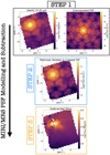 |
Fig. A.1. Scheme of the MIRI/MRS PSF modelling and subtraction applied to NGC 424 data. The arrow indicate the direction we followed during the PSF subtraction procedure. From left to right: A slice of MIRI Ch3 LONG data at the wavelength of the peak of the [Ne III] emission line with the corresponding slice of the oversampled WebbPSF cube. Step 2 and 3 represent the centred, rebinned, rotated and cropped PSF and the final PSF subtracted data slice. |
As was stressed at the beginning of this section, due to the wavelength-dependent PSF FWHM (Law et al. 2023; Argyriou et al. 2023; Bajaj et al. 2024) we used a tailored PSF model cube to subtract the PSF emission from all the 12 MIRI/MRS data cubes, repeating the detailed modelling described above to each slice of each data cube.
Appendix B: Electron density and dust attenuation maps
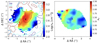 |
Fig. B.1. Spatially resolved estimate of the ionised gas electron density and dust attenuation in the circumnuclear region of NGC 424 obtained from the [SII]λλ6716,6731 doublet and Hα/Hβ ratio of MUSE data. Spaxels at S/N ≤ 5 are masked. Left panel: Red, cyan, and blue contours represent the 350, 325, and 300 km s−1 contours of the broad component of the [O III] velocity dispersion map shown in Fig. 6. North is up, east to the left. |
In this appendix we present the electron density estimate for the warm ionised gas obtained from the total intensities of the [Sii]λλ6716,6731 emission lines and the dust extinction map for NGC 424 making use of the Balmer decrement Hα/Hβ, assuming a Calzetti et al. (2000) attenuation law. In particular, to compute the electron density we used the [SII][6717]/[SII][6731] diagnostic line ratio (Osterbrock & Ferland 2006) from spaxels with S/N ≥ 5 on the total [SII]λλ6716,6731 emission lines, and assuming a typical value for the temperature of ionised gas of Te = 104 K.
Appendix C: Multi-phase kinematical maps of the MOKA3D fit
The best fit models obtained fitting with tailored MOKA3D modelling the multi-phase gas disc emission, as traced by H2S(1), [Ne III], CO (2-1), and [O III] emission lines, observed with MIRI, ALMA, and MUSE, respectively, are shown in this section. Details of the modelling are presented in Sect. 4.1 and the best-fit parameters are listed in Tab. 2. For more details on the MOKA3D modelling routine, see Marconcini et al. (2023) and Marconcini et al. (2025).
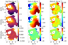 |
Fig. C.1. Comparison of the observed (top panel) and best-fit MOKA3D (middle panel) moment maps for the H2S(1) emission line. Residuals are shown in the bottom panel. The modelling and best-fit parameters are presented in Sect. 4.1 and listed in Tab. 2. North is up, east to the left. |
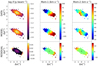 |
Fig. C.3. Continue of Fig. C.1 for the CO (2-1) emission line observed with ALMA. North is up, east to the left. |
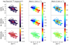 |
Fig. C.4. Continue of Fig. C.1 for the narrow component of the [O III] emission line observed with MUSE. North is up, east to the left. |
All Tables
MIR emission line fluxes from MIRI/MRS channels, in units of MegaJansky/steradians.
Best-fit parameters for the ionised outflow properties in NGC 424, traced by [Ne III] and [O III]λ5007 emission lines and inferred with the MOKA3D framework.
All Figures
|
Fig. 1. NGC 424 emission line images from MUSE WFM (left), ALMA (middle), and the point-source subtracted MIRI MRS Ch3 medium (right). The images were obtained integrating the total [O III]λ5007, CO (2-1), and [Ne V] emission lines, respectively. Blue square in MUSE image represents the ALMA FoV considered in this work. Orange, red, yellow, and white rectangles in ALMA image represent the FoVs of MIRI MRS Channels 1, 2, 3, and 4, respectively. Black crosses mark the nucleus position, determined as the peak of Hα emission from the MUSE data. North is up and east is left. |
| In the text | |
|
Fig. 2. MUSE (top panel) and MIRI MRS (bottom panel) integrated spectra for NGC 424 extracted from the same region, i.e. the MIRI MRS Ch 1 (orange square in Fig. 1). All the emission lines detected in each spectrum are highlighted. Warm molecular hydrogen transitions in the MIRI MRS spectrum are shown in blue. Black and purple spectra in the bottom panel represent the integrated MRS spectrum extracted from the entire FoV and from the 1 arcsec2 nuclear region of NGC 424, respectively. Red labels mark the positions of PAHs features at 11.25 and 12 μm. Grey spectrum in the bottom panel is the Spitzer IRS high-resolution extracted in full mode normalised to the MIRI MRS integrated spectrum. |
| In the text | |
|
Fig. 3. Multi-phase Gaussian fit of the [Ne III], H2S(1), [O III]λ5007, and CO (2-1) emission lines from MIRI/MRS, MUSE, and ALMA data cubes, respectively. Top left panel: [Ne III] emission tracing the redshifted ionised gas, obtained collapsing the flux in the spectral window 15.56–15.57 μm rest-frame from the PSF subtracted data cube (see Appendix A). White contours represent arbitrary [OIII] flux levels from MUSE data. North is up and east is left. Top right panels: Integrated [Ne III] and H2S(1) emission extracted from the black circular aperture of radius 0.6″, shown on the left panel. Bottom left: Integrated [O III]λ5007 emission and best-fit extracted from the same aperture shown in the top left panel. Bottom right: Integrated CO (2-1) emission extracted from spaxels with S/N ≥ 3, covering the nuclear region of NGC 424, as is shown in the bottom panel of Fig. 4. Data and total best-fit model are in black and red, respectively. The sum of the single Gaussian best-fit components is shown in blue (narrow), and orange (broad). Bottom panels show the residuals in green. Vertical dashed grey lines mark the rest-frame wavelength of the transitions. Data and best-fit are normalised to the peak of the observed spectrum. |
| In the text | |
|
Fig. 4. From top to bottom: NGC 424 disc emission traced by [Ne III], H2S(1), [OIII], and CO (2-1) emission lines. The disc emission is traced by the total line profile of the H2S(1) and CO (2-1) transitions and by the narrower Gaussian component for the [Ne III] and [O III] emission lines. From left to right we show the emission line integrated flux, line of sight (LOS) velocity and velocity dispersion maps corrected for instrumental broadening. The integrated logarithmic flux maps are in unit of MJy/sr, 10−20 erg/s/cm−2, and Jy/beam for MIRI, MUSE, and ALMA maps, respectively. The green and grey circles are the MIRI and MUSE PSF, respectively. The ALMA beam is represented as a magenta oval. From top to bottom, a S/N mask of 3, 3, 5, and 3 was applied to moment maps. MIRI moment maps are obtained from the emission line fitting of the point-source subtracted data cube. North is up and east is left. |
| In the text | |
|
Fig. 5. NGC 424 rotation curve inferred with MOKA3D using the H2S(1) (orange) and CO (2-1) (green) emission, and the narrow component of the [O III] (blue) emission line, from MIRI/MRS, ALMA, and MUSE, respectively. The rotation curve obtained fitting the narrow component of the [Ne III] shown in Fig. 4 is not reported, as the trend is similar to the H2S(1). The dotted black and grey curves represent the best-fit velocity profile of the DM (Eq. (3)) and baryonic matter (Eq. (2)), respectively. The total best-fit profile is shown as a solid red curve. The averaged rotating velocity and inclination values are listed in Table 2. Details on the MOKA3D disc model are discussed in Sect. 4.1. |
| In the text | |
|
Fig. 6. MOKA3D best-fit model for the ionised outflow traced by the broad component of the [O III] from MUSE data. Top panels: 3D reconstruction of the ionised gas clouds colour-coded based on their position with respect to the plane of the sky and observed along the outflow axis (left, i.e. as if the conical outflow axis coincide with the line of sight of the observed) and along the line of sight (right). The XY represents the plane of the sky, while the Z is the LOS. The dotted black lines in the right panel show the bi-conical outflow axis direction. According to the colourbar, blue and red clouds are blueshifted and redshifted, respectively. The bubble size is representative of the intrinsic cloud flux. Bottom panels: Data (top), MOKA3D best-fit (middle) and residual (bottom) moment maps, i.e. the integrated flux, the LOS velocity, and velocity dispersion maps. The residual maps are obtained by subtracting the model from the observed moment maps. Maps are masked at a S/N of 3. North is up and east is left. |
| In the text | |
|
Fig. 7. Same as in Fig. 6 for the [Ne III] emission line from MIRI MRS Ch3. Maps are masked at a S/N of 2. |
| In the text | |
|
Fig. 8. Multi-Gaussian fit of the integrated [Ne V] emission line from the total MIRI/MRS Ch3 MEDIUM band. Data and total best-fit model are in black and red, respectively. The narrow and broad Gaussian components are shown as solid blue and orange lines, respectively. The bottom panel shows the residuals in green. The vertical dashed grey line marks the rest-frame wavelength of the [Ne V] transition. |
| In the text | |
|
Fig. 9. Position-velocity diagrams extracted from a slit of width 0.8″ along the NGC 424 CO (2-1) kinematic minor axis (top panel, PA = 28°, see Table 2) and major axis (bottom panel, PA = 118°). CO (2-1) emission is masked at S/N ≤ 3. White contours correspond to arbitrary levels of the observed emission. Black contours correspond to arbitrary levels extracted from the best-fit model cube obtained with MOKA3D shown in Fig. C.3 and described in Sect. 4.1. |
| In the text | |
|
Fig. 10. Velocity channel maps at different velocity bins for the warm (H2S(1), top panels) and cold molecular (CO (2-1), bottom panels) gas components. Channel maps are in logarithmic scale and in units of MegaJansky/steradian (top panels) and Jansky/beam (bottom panel). Contours represent arbitrary flux level. Molecular gas knots in the galactic disc, discussed in Sect. 4.7, are labelled as C1, C2, and C3. North is up, east to the left. |
| In the text | |
|
Fig. A.1. Scheme of the MIRI/MRS PSF modelling and subtraction applied to NGC 424 data. The arrow indicate the direction we followed during the PSF subtraction procedure. From left to right: A slice of MIRI Ch3 LONG data at the wavelength of the peak of the [Ne III] emission line with the corresponding slice of the oversampled WebbPSF cube. Step 2 and 3 represent the centred, rebinned, rotated and cropped PSF and the final PSF subtracted data slice. |
| In the text | |
|
Fig. B.1. Spatially resolved estimate of the ionised gas electron density and dust attenuation in the circumnuclear region of NGC 424 obtained from the [SII]λλ6716,6731 doublet and Hα/Hβ ratio of MUSE data. Spaxels at S/N ≤ 5 are masked. Left panel: Red, cyan, and blue contours represent the 350, 325, and 300 km s−1 contours of the broad component of the [O III] velocity dispersion map shown in Fig. 6. North is up, east to the left. |
| In the text | |
|
Fig. C.1. Comparison of the observed (top panel) and best-fit MOKA3D (middle panel) moment maps for the H2S(1) emission line. Residuals are shown in the bottom panel. The modelling and best-fit parameters are presented in Sect. 4.1 and listed in Tab. 2. North is up, east to the left. |
| In the text | |
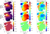 |
Fig. C.2. Continue of Fig. C.1 for the [Ne III] emission line. North is up, east to the left. |
| In the text | |
|
Fig. C.3. Continue of Fig. C.1 for the CO (2-1) emission line observed with ALMA. North is up, east to the left. |
| In the text | |
|
Fig. C.4. Continue of Fig. C.1 for the narrow component of the [O III] emission line observed with MUSE. North is up, east to the left. |
| In the text | |
Current usage metrics show cumulative count of Article Views (full-text article views including HTML views, PDF and ePub downloads, according to the available data) and Abstracts Views on Vision4Press platform.
Data correspond to usage on the plateform after 2015. The current usage metrics is available 48-96 hours after online publication and is updated daily on week days.
Initial download of the metrics may take a while.