| Issue |
A&A
Volume 701, September 2025
|
|
|---|---|---|
| Article Number | A224 | |
| Number of page(s) | 24 | |
| Section | Extragalactic astronomy | |
| DOI | https://doi.org/10.1051/0004-6361/202554812 | |
| Published online | 17 September 2025 | |
A new Bowen fluorescence flare and extreme coronal line emitter discovered by SRG/eROSITA
1
Max-Planck-Institut für extraterrestrische Physik, Giessenbachstraße 1, D-85748 Garching bei München, Germany
2
MIT Kavli Institute for Astrophysics and Space Research, 70 Vassar Street, Cambridge, MA, 02139
USA
3
Max-Planck-Institut für Astrophysik, Karl-Schwarzschild-Straße 1, 85748 Garching bei München, Germany
4
JILA, University of Colorado and National Institute of Standards and Technology, 440 UCB, Boulder, 80308 CO, USA
5
Department of Astrophysical and Planetary Sciences, 391 UCB, Boulder, 80309 CO, USA
6
Centre for Astrophysics Research, University of Hertfordshire, College Lane, Hatfield, AL10 9AB
UK
7
European Southern Observatory, Karl-Schwarzschild-Strasse 2, 85748 Garching bei München, Germany
8
Millennium Institute of Astrophysics (MAS), Nuncio Monseñor Sotero Sanz 100, Of. 104, Providencia, Santiago, Chile
9
Dipartimento di fisica e Astronomia, Università degli Studi di Padova, Vicolo dell’Osservatorio 3, 35122 Padova, Italy
10
International Center for Radio Astronomy Research, Curtin University, GPO Box U1987, Perth, WA, 6845
Australia
11
Astronomical Observatory, University of Warsaw, Al. Ujazdowskie 4, 00-478 Warszawa, Poland
12
Leibniz-Institut für Astrophysik Potsdam, An der Sternwarte 16, 14482 Potsdam, Germany
13
South African Astronomical Observatory, PO Box 9 Observatory Rd, 7935 Observatory, Cape Town, South Africa
14
Department of Astronomy, University of Cape Town, Private Bag X3, Rondebosch, 7701
South Africa
15
Department of Physics, University of the Free State, PO Box 339 Bloemfontein, 9300
South Africa
16
Las Campanas Observatory – Carnegie Institution for Science, Colina el Pino, Casilla 601, La Serena, Chile
⋆ Corresponding author: This email address is being protected from spambots. You need JavaScript enabled to view it.
Received:
27
March
2025
Accepted:
4
July
2025
Abstract
The nuclear X-ray transient eRASSt J012026.5−292727 (J012026 hereafter) was discovered in the second SRG/eROSITA all-sky survey (eRASS2). The source appeared more than one order of magnitude brighter than the eRASS1 upper limits (peak eRASS2 0.2–2.3 keV flux of 1.14 × 10⁻¹² erg cm−2 s−1) and with a soft X-ray spectrum (photon index of Γ = 4.3). Over the following months, the X-ray flux started decaying and demonstrated significant flaring activity on both short (hour) and long (year) timescales. By inspecting the multiwavelength light curves of time-domain wide-field facilities, we detected a strong mid-infrared flare, which evolved over two years, and a weaker optical counterpart, with possible hints of a rise > 3 years prior to the X-ray discovery. Follow-up optical spectroscopy revealed transient features, including redshifted Balmer lines (FWHM of ∼1500 km s−1), strong Fe II emission, He II, Bowen fluorescence lines, and high-ionization coronal lines such as [Fe X] and [Fe XIV]. One spectrum displayed a triple-peaked Hβ line, consistent with emission from a face-on elliptical accretion disk. The spectroscopic features and the slow evolution of the event place J012026 within the nuclear-transient classifications of Bowen fluorescence flares (BFFs) and extreme coronal line emitters (ECLEs). BFFs have been associated with rejuvenated accreting supermassive black holes, although the mechanism triggering the onset of the new accretion flow is yet to be understood, while ECLEs have been linked to the disruption and accretion of stars in gas-rich environments. The association of J012026 with both classes, combined with the X-ray, multiwavelength, and spectroscopic information, supports the idea that the BFF emission could be, at least in some cases, triggered by tidal disruption events (TDEs) perturbing gaseous environments. The observed short- and long-term X-ray variability, uncommon in standard TDEs, adds complexity to these families of nuclear transients. These results highlight the diverse phenomenology of nuclear accretion events and demonstrate the value of systematic X-ray surveys, such as eROSITA and Einstein Probe, for uncovering such transients and characterizing their physical origin.
Key words: Galaxy: nucleus / galaxies: active / galaxies: nuclei
NASA Einstein fellow.
© The Authors 2025
 Open Access article, published by EDP Sciences, under the terms of the Creative Commons Attribution License (https://creativecommons.org/licenses/by/4.0), which permits unrestricted use, distribution, and reproduction in any medium, provided the original work is properly cited.
This article is published in open access under the Subscribe to Open model.
Open access funding provided by Max Planck Society.
1. Introduction
When a star wanders too close to a supermassive black hole (SMBH), tidal forces can rip it apart. If the disruption occurs outside the event horizon, as matter falls toward the black hole, a flare of optical/UV/X-ray radiation will appear and last on a timescale of months (Hills 1975; Rees 1988; Evans & Kochanek 1989; Phinney et al. 1989). These so-called tidal disruption events (TDEs) can illuminate dormant nuclear black holes, complementing the population revealed by active galactic nuclei (AGN). As they predominantly happen around low-mass SMBHs or even the elusive intermediate-mass black holes, TDEs are crucial for a complete black hole demographic analysis (e.g., Stone & Metzger 2016). TDEs are also the perfect environment to study the onset, development, and exhaustion of accretion flows and related ejections, such as jets and outflows. Since their overall evolution occurs within a few years, all their phases can be probed accurately.
The first TDE candidates were discovered in the X-rays with the ROentgen SATellite (ROSAT; Trümper 1982; Komossa & Greiner 1999; Komossa & Bade 1999; Grupe et al. 1999; Greiner et al. 2000) as soft X-ray flares decaying over a few months, following the characteristic t−5/3 shape, which can be derived from simple theoretical arguments (see, e.g., Saxton et al. 2020; Gezari 2021). In the following years, a few more sources were discovered serendipitously with Chandra, XMM-Newton, and Swift (Weisskopf et al. 2000; Jansen et al. 2001; Gehrels et al. 2004, and see Komossa 2015 and references therein). That said, in the past two decades, most events have been selected in the optical/UV thanks to the advent of wide-field time-domain surveys, such as the Panoramic Survey Telescope and Rapid Response System (Pan-STARRS; Chambers et al. 2016), the Palomar Transient Factory and its successor the Intermediate Palomar Transient Factory (iPTF; Law et al. 2009; Kulkarni 2013), the All-Sky Automated Survey for Supernovae (ASAS-SN; Shappee et al. 2014; Kochanek et al. 2017), the Asteroid Terrestrial-impact Last Alert System (ATLAS; Tonry et al. 2018), and the Zwicky Transient Facility (ZTF; Bellm et al. 2018).
However, the interplay of optical/UV and X-ray radiation is a crucial element in our attempts to understand the physical origin of the radiation in TDEs. In fact, while it is generally understood that the X-ray emission arises due to accretion processes, it is still unclear where the optical/UV radiation comes from. Moreover, many optically selected TDEs do not show X-ray emission up to ∼100 days after the optical peak (e.g., Guolo et al. 2024a). Currently, two main families of models have been proposed: the first proposes that the primary X-ray radiation from the accretion disk is reprocessed to longer wavelengths by a thick envelope (e.g., Guillochon et al. 2014; Roth et al. 2016; Metzger & Stone 2016; Parkinson et al. 2022). In contrast, the second model proposes that the optical/UV emission is due to shocks created by collisions between incoming and outgoing streams on highly eccentric orbits near the apocenter of the returning stream (e.g., Piran et al. 2015; Shiokawa et al. 2015; Jiang et al. 2016; Bonnerot et al. 2017; Ryu et al. 2023; Steinberg & Stone 2024). In the latter scenario, the accretion disk can only form after the dissipation of orbital energy through the self-crossing shocks, naturally explaining the delayed emergence of X-rays with respect to the optical flare. The cross-correlation of optical and X-ray light curves has provided evidence to support this scenario (e.g., Guo et al. 2025); however, when early X-ray sampling was available, observations revealed a more complex picture, with the notable example of AT 2022dsb showing fading X-rays prior to the optical peak (Malyali et al. 2024). Because of this, assembling an unbiased sample, with events selected both in the X-rays and in the optical/UV bands, is critical for drawing a clearer picture of the physical mechanism behind these transients.
The systematic selection of events in the X-rays has been greatly enhanced by the extended ROentgen Survey with an Imaging Telescope Array (eROSITA; Predehl et al. 2021), the soft X-ray instrument on board the Spektrum–Roentgen–Gamma (SRG; Sunyaev et al. 2021). By scanning the entire sky once every six months, between four and five times, eROSITA has provided the largest sample of systematically selected TDEs (13 in Sazonov et al. 2021, six in Khorunzhev et al. 2022, and 31 in Grotova et al. 2025b) and has discovered unique and exotic sources, such as AT 2019avd, eRASSt J133157.9−324321, eRASSt J045650.3−203750, eRASSt J234402.9−352640, and AT 2022dsb (respectively, Malyali et al. 2021, 2023b; Liu et al. 2023; Homan et al. 2023; Malyali et al. 2024).
Now that the gap between selection techniques is being filled, with over a hundred TDEs discovered, the diversity within these events is becoming increasingly apparent. Some events show only either X-rays or optical/UV variability (e.g., Grotova et al. 2025b; Gezari et al. 2012), while others show repetitions or re-brightenings (e.g., Malyali et al. 2023b; Guolo et al. 2024b), quasi-periodic phenomena (quasi-periodic oscillations; e.g., Reis et al. 2012; Pasham et al. 2014, quasi-periodic ultrafast outflows; e.g., Pasham et al. 2014, and quasi-periodic eruptions; e.g., Miniutti et al. 2019; Giustini et al. 2020; Arcodia et al. 2021), and a general deviation from a t−5/3 behavior (e.g., Guolo et al. 2024a). Additionally, some other classes of nuclear transients have been connected to the presence of TDEs. This is the case for extreme coronal line emitters (ECLEs; e.g., Komossa et al. 2008; Wang et al. 2012), which show strong and transient high-ionization coronal lines in optical spectra, such as [Fe X] λ6376, [Fe XI] λ7894, [Fe XIV] λ5304, and [S XII] λ7612, which correspond to ionization potentials in the hundreds of eV. Although these lines can also be produced in AGN, ECLEs are distinguished by their extreme ratios of coronal line emission to typical AGN lines, such as [O III] λ5007, and by a lack of evidence of strong ongoing nuclear activity (e.g., Cerqueira-Campos et al. 2021; Negus et al. 2021; Prieto et al. 2022). ECLEs are also characterized by monotonically decaying optical light curves, similarly to TDEs but on longer timescales (years vs. months; e.g., Newsome et al. 2024). The transient behavior of both the continuum and the coronal lines and rate estimates that align with those of TDEs (Wang et al. 2012) strongly suggest that ECLEs are powered by TDEs in gas-dense environments, where the flaring UV and soft X-ray radiation can ionize nearby gas, producing the observed line emission (Hinkle et al. 2024). Indeed, the emergence of transient coronal lines after the dust-reprocessing echo in the TDE AT 2017gge (Onori et al. 2022) first observationally confirmed this scenario, and a similar behavior has been observed in AT 2019qiz (Short et al. 2023), strengthening the connection.
Another transient class potentially associated with TDEs is the one identified in Trakhtenbrot et al. 2019 and dubbed Bowen fluorescence flare (BFFs) in Makrygianni et al. 2023. These events show strong He II and N III emission, which is also commonly seen in TDEs (e.g., Onori et al. 2019; Leloudas et al. 2019; Blagorodnova et al. 2019; van Velzen et al. 2021a) and is produced with the Bowen fluorescence mechanism (Bowen 1928), but with widths on the order of 103 km s−1, compared to the typical 104 km s−1 in TDEs (e.g., Arcavi et al. 2014). Similarly to ECLEs, they also decay on overall longer timescales, with power-law slopes flatter than the typical t−5/3 (Trakhtenbrot et al. 2019). BFFs have been associated with “rejuvenated SMBHs” (Trakhtenbrot et al. 2019), in which the emission originates from a suddenly illuminated preexisting broad line region (BLR), where the sudden increase in the extreme UV/X-ray continuum triggers the Bowen fluorescence mechanism. Some of these events show clear indications of previous AGN activity (e.g., Makrygianni et al. 2023; Frederick et al. 2021; Ŝniegowska et al. 2025), but the rejuvenation mechanism is not clear, and a TDE connection has been proposed for events AT 2019aalc and AT 2022fpx (Veres et al. 2024; Koljonen et al. 2024).
In this work we present the new eROSITA-selected transient eRASSt J012026.5−292727 (hereafter J012026), which was missed by optical surveys and adds a new piece to the puzzle of TDEs, their non-monotonic X-ray light curves, gas-rich environments, and their connections with ECLEs and BFFs. The paper is structured as follows: In Sect. 2 we describe the discovery of J012026, and in Sect. 3 we describe the X-ray data and their reduction, analysis, and results. In Sect. 4 we describe the photometric properties, and in Sect. 5 the optical spectroscopy. We present the discussion on the nature of the source in Sect. 6 and summarize our results and conclusions in Sect. 7. Throughout this paper we adopt a flat Λ cold dark matter cosmology, with H0 = 67.7 km s−1 Mpc−1, and Ωm = 0.309 (Planck Collaboration XIII 2016).
2. Discovery and follow-up
J012026 was discovered as a new bright source on 2020-06-13 during the second eROSITA all-sky survey (eRASS2; see Grotova et al. 2025a for details on the search for non-AGN nuclear transients in eROSITA). The new soft and point-like source was localized at RA = 20.1107°, Dec = −29.4631°, consistent with the nucleus of the z = 0.1029 galaxy 2dFGRS TGS295Z163 (Colless et al. 2001) (see Fig. 1). Independently, J012026 was picked up by the blind quasi-periodic eruption (QPE) search algorithm described in Arcodia et al. 2024 due to its short-term variability in eRASS5 (see Sect. 3). Following the discovery, several Swift/X-ray telescope (XRT) observations were requested (see Table 1) and the source was sporadically monitored until 2024. To further investigate the short-term X-ray variability, a 53 ks XMM-Newton observation was later performed, and the source was also monitored every ∼1 hour for about three days with Swift/XRT in September 2024. Shortly after, an Einstein Probe (EP; Yuan 2022) Follow-up X-ray Telescope (FXT) observation of J012026 was performed as part of an eROSITA TDE follow-up program. The multiwavelength light curve of J012026 can be seen in Fig. 2.
X-ray observation log of J012026.
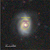 |
Fig. 1. LS10 grz-color image of the host galaxy of J012026. The purple circle indicates the eRASS2 positional error, and the yellow circle the Swift/XRT positional error. |
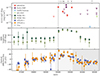 |
Fig. 2. Multiwavelength light curve of J012026. Top panel: X-ray evolution in the 0.2–2.3 keV band (empty triangles correspond to upper limits). Middle panel: WISE W1 and W2 light curve presented in AB magnitudes. Bottom panel: Difference-photometry light curve for the ATLAS o and c filters in μJy. The vertical dashed lines indicate the eRASS2 discovery. The numbered ticks at the top of the plot indicate the epochs at which optical spectroscopy was collected (see Sect. 5). |
J012026 was also monitored in a multiwavelength fashion. Several follow-up optical spectra were obtained between 25 days after the discovery and 2024, as discussed in Sect. 5. Moreover, J012026 was observed in radio bands with the Australia Telescope Compact Array (ATCA) in three different epochs; however, the detections were marginal (see Appendix B).
3. X-ray data and analysis
3.1. eROSITA
J012026 was detected in eRASS2, 3, 4, and 5, but not in eRASS1. We retrieved the eRASS1 upper limits from the eROSITA DR1 upper limit server1 (Tubín-Arenas et al. 2024; Merloni et al. 2024). For the remaining all-sky surveys, we used the light curves and spectra systematically extracted from the eROSITA processed event files (version 020) with the task SRCTOOL of the eROSITA science analysis software (eSASS v.211214.05; Brunner et al. 2022). We combined light curves and spectra collected from telescope modules (TMs) 1, 2, 3, 4, and 6, as TM5 and TM7 are affected by light leaks (Predehl et al. 2021). The circular extraction region sizes scale with the maximum likelihood source count rate reported in the catalogs and have radii of 85″, 58″, 51″, and 84″, respectively, for eRASS2, 3, 4, and 5. The background extraction regions were determined as described in Liu et al. (2022).
The eROSITA scanning strategy is such that each point of the sky is observed repeatedly for up to 40 seconds every four hours, i.e., every eROday (Predehl et al. 2021). The number of exposures depends on the ecliptic latitude but has a typical value of 6. This implies that for each eRASS, a light curve of ∼1 day of baseline can be extracted. The eROSITA eROday X-ray light curve of J012026 is presented in Fig. 3, with the exclusion of eRASS1, as the source is undetected. It can be seen that eRASS3 and eRASS5 show large amplitude eROday variability, with flaring activity present respectively on the seventh (eRASS3) and third and seventh (eRASS5) eROdays. The identification of the flares was initially visual and later confirmed by calculating the significance of the variability through the maximum amplitude deviation (MAD) method (Boller et al. 2016). We conservatively computed the amplitude of the variation between the count rate (C) of the flaring eROday (tflare) and the eROday with the lowest count rate (tmin) in the same eRASS as
 (1)
(1)
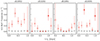 |
Fig. 3. eROSITA eROday 0.2–2.0 keV band light curve of J012026. The empty red circles show the source vignetting and exposure corrected count rates, while the gray triangles correspond to the background count rate. The filled red circles correspond to the eROdays selected as flaring. The time (x) axis is in units of days since the first observation of the source, for each scan. |
where σlow and σupp are respectively the lower and upper 1σ errors. The significance of the variability can be computed as
 (2)
(2)
As shown in Buchner et al. (2022), the value of SIG_MAD is an underestimation of the true significance of the variability. In their work, they report values of SIG_MAD corresponding to 3σ significance at a given average count rate. Based on Fig. 13 of Buchner et al. (2022), we adopted a 3σ threshold of 1.5 for J012026. We measure SIG_MAD = 1.6 for eRASS3, and 2.4 and 2.0, respectively, for the first and second eRASS5 flares.
We analyzed eRASS2-5 spectra with the Bayesian X-ray Analysis (BXA) software version 4.1.2 (Buchner et al. 2014), which connects the nested sampling algorithm UltraNest (Buchner 2019, 2021) with the fitting environment CIAO/Sherpa (Fruscione et al. 2006). Spectra were fit unbinned and using C-statistics. The fitting procedure included a principal-component-analysis-based background model (e.g., Simmonds et al. 2018) derived from a large sample of eROSITA background spectra (Liu et al. 2022).
For all spectra, we fit both a multicolor disk model (DISKBB) and a power-law model (POWERLAW), as shown in Fig. A.4. In both cases, we included the contribution of Galactic absorption through the model TBABS, which is due to a line-of-sight column density of NH = 1.44 × 1020 cm−2, as estimated by the HI4PI collaboration (HI4PI Collaboration 2016).
To test a potential spectral evolution in conjunction with the flares in eRASS3 and eRASS5, we repeated the spectral analysis by first separating the flares from the rest of the respective eRASS. We isolated the third eROday in eRASS3 and the third and seventh eROday in eRASS5 with the eSASS task EVTOOL. We then combined the two eRASS5 flares into a single spectrum, to maximize counts, and then repeated the fitting procedure four times, respectively on the eRASS3 flare, the eRASS5 flares, and the remaining “baseline” counts in eRASS3 and in eRASS5.
The results of our fit are reported in Table 2, and the spectra can be visualized in Appendix A.2. Both models reproduce the data well for all observations, although a comparison of Bayesian evidence suggests that a power-law model is preferred in eRASS2 and for the eRASS3 flare. However, the evidence is not decisive (see Kass & Raftery 1995), and a visual inspection of the spectra in Appendix A.2 does not show a significantdifference between the two models. eRASS4 shows a drastically different spectral shape compared to the other observations. Since this observation corresponds to the lowest flux state, with a total of 12 source+background counts in the 0.2–2.3 keV band, we do not consider this variation to be physical.
Spectral fit results for the eROSITA and Swift/XRT observations of J012026.
Excluding eRASS4, there is no drastic spectral variation among eROSITA all-sky surveys. However, there is mild evidence of a general harder-when-brighter behavior, which is discussed jointly with the Swift/XRT observations in the next section.
We note that J012026 is located at a distance of 60″ from the known AGN WISEA J012025.95−292637.3. The latter was detected by the eROSITA pipeline only in eRASS1 Merloni et al. 2024), while it was not found in later epochs (see also Fig. A.3). In Appendix A.1 we show through a more conservative extraction procedure that, if present, contamination from WISEA J012025.95−292637.3 is negligible.
3.2. Swift/XRT
J012026 was observed with Swift/XRT seven times before 2024 and every hour for three days in 2024 (see Table 1), all in photon-counting mode. The XRT light curves and spectra were generated and downloaded from the UK Swift Science Data Centre website (Evans et al. 2007, 2009). We binned the light curves before 2024 by snapshot and the observations taken in 2024 by one day to derive meaningful upper limits. The source was detected only in observations 00014018003 and 00014018004 (Swift/XRT3 and Swift/XRT4 hereafter; see Table 1). We computed flux upper limits for all other observations by assuming a DISKBB model with Tin = 100 eV and assuming that the emission is due to an accretion disk (see the discussion in Sect. 6).
We analyzed the spectra of Swift/XRT3 and Swift/XRT4 following the same prescription as for the eROSITA data. We report the results in Table 2, and we note that the peak luminosity of the Swift/XRT detections is similar to the eROSITA flares. In Swift/XRT4, the power-law model is statistically more favored than the DISKBB, but, similarly to the eROSITA observations, a visual inspection does not show any particular preference (see Fig. A.4).
As mentioned in the previous section, the eROSITA and Swift-XRT spectral analysis reveals a general harder-when-brighter behavior. In Fig. 4 we plot the 0.2–2.3 keV flux versus the photon index (Γ) for eRASS2, the eRASS3 and eRASS5 baselines and flares, and Swift/XRT3 and 4. We overplot a linear fit, which suggests an anticorrelation; however, the 95% confidence interval, derived from Monte Carlo iterations accounting for uncertainties in both variables, is consistent with no correlation, as shown by the gray band. We also computed the distribution of the Pearson correlation coefficient in an analogous Monte Carlo fashion, and confirm the lack of statistical significance of the anticorrelation (the details of this test are presented in Appendix A.2).
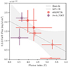 |
Fig. 4. 0.2–2.3 keV flux vs. spectral photon index for X-ray detections. Filled red markers correspond to eROSITA flaring states and empty markers to the baseline spectra. We do not include eRASS4 due to its low flux level. |
3.3. XMM-Newton
XMM-Newton observed the location of J012026 as a target of opportunity on December 31, 2023 (see Table 1). No source was detected at the position of J012026. The observation data files were reduced using the XMM-Newton Science Analysis System (SAS) software (version 21.0; Gabriel et al. 2004), with the latest available calibration files. We generated the event lists for the European Photon Imaging Camera (EPIC) MOS (Turner et al. 2001) and pn (Strüder et al. 2001) detectors through the SAS tasks EMCHAIN and EPCHAIN. We identified periods of high background flaring and filtered the event lists accordingly, resulting in an effective exposure time of 40 215 s. We extracted counts at the J012026 two-degree-field (2dF) source position for all three cameras with circular regions with radii of 20″ and background counts from circular regions with radii of 45″. We estimated the 3σ flux upper limit by calculating the Poissonian confidence interval and assuming a DISKBB model with Tin = 100 eV, consistently with the Swift/XRT upper limits. This results in a 3σ upper limit in the 0.2–2.3 keV band of f < 3.3 × 10⁻¹⁵ ergs/s/cm2.
3.4. Einstein Probe/FXT
The 2024-10-11 EP/FXT observation yielded no detection (see Table 1). We used the pipeline FXTCHAIN of the FXT Data Analysis Software (FXTDAS) v.1.1, to produce clean event files. We derived upper limits for the two TMs, FXT-A and FXT-B (Yuan et al. 2025), by extracting photon counts from a source circular region with radius 30″, a background region ten times larger, and assuming the same DISKBB model with kT = 100 eV. The respective FXT-A and FXT-B 3σ flux upper limit in the 0.2–2.3 keV band are f < 2.3 × 10⁻¹⁴ ergs/s/cm2 and f < 3 × 10⁻¹⁴ ergs/s/cm2.
4. Photometry
4.1. Mid-infrared variability
The location of J012026 has been observed since 2013 twice per year as part of the near-earth object wide-field infrared survey explorer (NEOWISE) reactivation mission (NEOWISE-R; Mainzer et al. 2014). We obtained the NEOWISE-R light curve from the NASA/IPAC Infrared Science Archive (IRSA), using the Table Access Protocol (TAP) service2 by compiling all source detections within 2″ of the position of the host-galaxy nucleus. We re-binned individual flux measurements to one point every six months for all-sky scans and converted them into magnitudes (see Fig. 2, middle panel). The historic mid-infrared (MIR) light curve of J012026 was flat until 58 823 but exhibited a significant brightening of ∼0.5 mag in W1 and ∼0.7 mag in W2 at the time of the eRASS2 detection (marked with a vertical dashed line in Fig. 2). The light curve plateaued for ∼2 years until MJD 59758, after which it decayed back to the quiescent level. The pre-flare W1 − W2 color was −0.26 mag (0.4 in the Vega system) but reddened to −0.04 mags (0.6 Vega mags) during the outburst, closer to the AGN color selection (e.g., 0.8 in the Vega system; Stern et al. 2012; Assef et al. 2013)
4.2. Optical variability
We searched for an optically variable counterpart by obtaining the ATLAS light curve through the forced photometry service3 (Tonry et al. 2018; Smith et al. 2020; Shingles et al. 2021). ATLAS uses two 0.5-m telescopes in Hawaii (Haleakala and Mauna Loa Observatory) to cover roughly a quarter of the sky per night, obtaining images in two broadband filters, c and o, covering respectively 420–650 and 560–820 nm. We present the difference point spread function photometry in Fig. 2, bottom panel, binned by 45 days to obtain meaningful detections, by adapting the software provided by Young 20204.
We notice that the source significantly increased in flux before MJD 58000. Moreover, close to the eRASS2 detection, we observe a significant rise, especially in the o band. Lastly, the emission decays and then plateaus on timescales comparable to the MIR flare. We note that the reference template image used to perform difference photometry is periodically replaced by the forced photometry service. The epochs corresponding to different templates are marked in Fig. 2 with different shades of gray. Since the change of templates occurred during the rise and during the decline of the optical transient, as retrieved from the light-curve files, it is not possible to determine whether the plateau is at a level compatible with pre-58000 or with the 58000-eRASS2 level.
4.3. Host galaxy properties
As shown in Fig. 1, the host-galaxy of J012026 is a spatially resolved, face-on spiral galaxy with possible hints of a bar. To derive its properties, we compiled the MIR-to-near UV spectral energy distribution (SED) of J012026 using the tool RainbowLasso5, released in conjunction with the SED-fitting code Genuine Retrieval of AGN Host Stellar Population (GRAHSP; Buchner et al. 2024). The tool retrieves near-UV magnitudes from the Galaxy Evolution Explorer (GALEX; Bianchi et al. 2017), and optical (g, r, i, z) and WISE (W1 − W4) fluxes from Legacy Survey data release 10 (LS10; Dey et al. 2019). Given the large extent of the host galaxy of J012026, we chose to use aperture photometry. After visually inspecting the azimuthal brightness profiles, we selected apertures of 7″ for the DECam filters g, r, i, and z, and 9″ for the W1 − W4 filters. For GALEX, we took the total flux.
We then modeled the SED using GRAHSP, including both stellar and nebular components, attenuated by dust and redshifted. The best-fit solution corresponds to a stellar mass of log(M*/M⊙) = 11 ± 0.1 and a star formation rate of 5 ± 1 M⊙ yr−1. By using the scaling relations presented in Reines & Volonteri 2015, we obtain a black hole mass of 107.5 ± 0.5 M⊙. The observed and modeled SED is shown in Fig. 5.
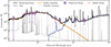 |
Fig. 5. Observed and modeled SED of J012026. The purple squares represent, respectively, the GALEX, DECam g, r, i, z, and W1 − W4 observed fluxes, while the red dots represent the model-predicted fluxes. The orange, gray, and blue lines represent the best-fit individual model components, which are respectively stellar, nebular, and dust emission. The black line is the total best-fit model. |
5. Optical spectroscopy
5.1. Spectroscopic observations
Seven optical spectroscopic observations were performed, starting 25 days after the eRASS2 discovery, and lasting ∼ four years. Additionally, an archival spectrum taken as part of the 2dF survey in 2001 is available. A log of the observations is presented in Table 3, and a description of the data reduction is presented in Appendix C. Both of the South African Large Telescope (SALT) Robert Stobie Spectrograph (RSS) spectra have been observed in long-slit mode, with a resolution of R ∼ 1200 at 5600 Å. The WiFes observations are performed using the R3000 and B3000 gratings, which correspond to a spectral resolution of R ∼ 3000 in both the blue and red arms. For the Baade Inamori-Magellan areal camera & spectrograph (IMACS) observation, we used the Grism 300 with a slit of 0.7″, and for the Clay low dispersion survey spectrograph (LDSS3)observation, we used the VPH-All grating with a 1″ slit. For the New Technology Telescope (NTT) EFOSC2 observations, we used the grating Gr#13 with a 1.2″ slit. Lastly, for the Baadee/Magellan Echellette (MagE) observations, we used a 0.5″ slit. In the following text, we refer to the observation by the ID number reported in Table 3.
Spectroscopic observations of J012026.
We recomputed the redshift of J012026 by fitting two Gaussian functions to the Ca II H & K absorption doublet for the two SALT/RSS spectra (1 and 5), and by fitting one Gaussian function to the [OIII] emission line in spectra 1, 3, and 5. We did so by using the lmfit Python package, which employs a Levenberg-Marquardt algorithm to fit the data (Newville et al. 2016). The results converge to a redshift of z = 0.1029. The rest-frame optical spectra of J012026 are shown in Fig. 6. Interestingly, J012026 is characterized by a number of peculiar spectral features, such as: (1) redshifted Balmer lines with a full width at half maximum (FWHM) of ∼1500 km s−1, (2) a strong Fe II complex, (3) He II and N III lines, (4) high-ionization coronal lines, and (5) a triple-peaked Hβ. In the following sections, we accurately describe the analysis performed on these observations and the characterization of the features. The implications of our results are later discussed in Sect. 6.
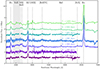 |
Fig. 6. Normalized rest-frame follow-up spectra of J012026, offset by an arbitrary factor for visualization purposes. The most significant emission lines are indicated with dashed lines, and the gray-shaded area shows the prominent Fe II complex. Above each spectrum, we report the ID and phase since the eRASS2 discovery in days. |
5.2. Continuum removal
Given that the spectra were obtained with different instruments and processed following different prescriptions, we first normalized them to their rest-frame 5900–6200 Å median flux. We chose this wavelength range as it is covered by all spectra, it is line-free, and it is less affected by the flare emission, which is more prominent at bluer wavelengths. We did not apply any Galactic reddening correction, as the color excess measured toward J012026 has a value of E(B − V) = 0.015, as obtained from the dust maps of Schlafly & Finkbeiner 2011. This would correspond to a flux correction < 5%, which we consider negligible.
We then removed the continuum contribution in order to model the residual emission lines. The continuum emission is the combination of the host galaxy, a strong Fe II complex emission, and a blue excess due to the transient flare. We subtracted the host contribution by using the archival 2dF spectrum, calibrated using the average response function from Lewis et al. (2002). We then modeled the spectrum with the code pPXF (Cappellari 2023) using the stellar population synthesis models of Conroy & Gunn (2010). By doing so, we were able to interpolate in a physically motivated fashion the low-resolution 2dF spectrum to the higher resolution follow-up spectra, and to remove the contributions of the artifacts. The subtraction is performed after interpolating the 2dF template to the target spectrum resolution and minimizing the normalized flux difference in the 5900–6200 range. An example of the procedure is shown in the left panel of Fig. C.2.
After subtracting the host, we fit each spectrum with a power law in the line-free regions 4000–4100 Å, 5400–5500 Å, and 5900–6200 Å. For each spectrum, both normalization and slope were left free to vary. After removing the contribution of the power law, we fit the Fe II template presented in Park et al. 2022 on the residual spectrum over the whole 4000–5600 range. The Fe II template is convolved with a Gaussian kernel, of which the width is left as a free parameter to allow for line broadening. The normalization and line centroids of the Fe II template are left as free parameters. After a best-fit solution is found and the results are visually inspected, we subtracted the Fe II template. An example of this procedure is shown in the right panel of Fig. C.2.
5.3. Emission line analysis
We modeled residual emission lines with a combination of Gaussian functions by using the lmfit Python package, as for the redshift estimation. For each spectrum, we first visually identified which lines are present, and later we fit them with one to four Gaussian, depending on how significantly the chi-square improves when adding one more component. To quantify the systemic shift and width of the lines in a consistent way, we used the centroid and FWHM resulting from the single Gaussian fit, while to fully characterize the flux, we combined the contribution of all significant Gaussians. Two examples of this fitting procedure can be seen in Fig. C.3.
Spectrum 1 shows clear Hβ and Hγ emission (Hα is out of the observed spectral range) along with He I 5876 Å, the high-ionization “coronal” lines [Fe X] λ6375 and [Fe XIV] λ5303, He II λ4686, and [OIII] λ5007. We note here that the Balmer lines are significantly redshifted with respect to the emission from the other lines and, specifically, from the [OIII]. This feature will stay consistent in all spectra, and it will be carefully discussed in Sect. 6. Spectrum 2 has a higher resolution but lower S/N ratio. Therefore, we re-binned it by a factor of 4. We observe the same line as spectrum 1 below 5500 Å (He I is not detected, and [Fe X] is outside of the observed spectral range), and tentatively detect the presence of the N III λ4641 emission complex. We also note that the [Fe XIV] appears particularly pronounced and broad. This could be due to a blending with [Fe VII] λ5276. In fact, in all spectra, the FWHM of the [Fe XIV] line is > 4000 km s−1, a factor of > 2 compared to all other emission lines, and it is centered at 5292 ± 2 Å, in between the central wavelengths of [Fe VII] and [Fe XIV]. However, we note that the S/N of this feature in all spectra is not high enough to allow for an accurate analysis. Spectrum 3, extending to longer wavelengths, is also able to reveal the presence of a strong Hα line in addition to the aforementioned features, which are also detected in the following spectrum 4. In addition, in spectra 3 and 4, we confirm the detection of N III. In spectrum 5, we observe a unique feature that is not present in any other spectra, namely a triple-peaked Hβ, while still noting the presence of all aforementioned features. We discuss the modeling and interpretation of this feature in Sect. 5.4. Spectra 6 and 7 appear similar to the other spectra covering the Hα range, although spectrum 7 has a lower S/N, and due to the re-binning, we can no longer confidently identify [Fe X], [Fe XIV](+[Fe VII]), He I and He II. We also note that the Hβ amplitude is now comparable with the [OIII].
In a more quantitative fashion, we report the fit results for all spectra in Table C.1, and we plot the results of our analysis in Fig. 7. In the two left panels, we show the temporal evolution of the line velocity offset (top panel) and FWHM (bottom panel) of the main modeled lines, excluding spectrum 5 because of the triple-peaked Hβ. In the two right panels, instead, we plot the evolution of emission line ratios. Because of the potential blending, we excluded the [Fe XIV]+[Fe VII] feature from this analysis.
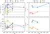 |
Fig. 7. Line parameter evolution of J012026. In the top-left panel, we plot the limit on the velocity resolution of the follow-up spectra with dotted lines. In the top-right panel, we plot the theoretical values of an unobscured system of the corresponding color ratios with dotted lines. |
From the top left panel, we can observe that all Balmer lines are redshifted with respect to the [OIII] expected rest-frame wavelength at all epochs. The Hγ velocity offset appears to vary between the first and second epoch from 300 km s−1 to 500 km s−1, but we argue that this could be an effect of Fe II subtraction, which affects this emission line the most. In general, the shift of the Balmer lines is between 300 and 600 km s−1 and is also seen in the He I line. The He II, N III, and [Fe X] instead, are always consistent with a shift of less than 200 km s−1 within the errors, a lower limit on the velocity resolution of our spectra, making this consistent with no systemic offset, and suggesting the presence of two separate kinematic components.
The bottom left panel, showing the FWHM evolution for the same lines, supports the kinematic disjunction of the He II with respect to the lower-ionization energy Balmer, He I and N III lines. We again argue that the apparent variations of the Hγ profile in the first epoch is likely due to the degeneracy of the emission line with the Fe II complex. Additionally, we also argue that the anticorrelated variation in the He II and N III profiles in spectrum 6 could also arise due to the low wavelength separation of the two features, which adds a degree of degeneracy. In fact, due to the modest resolutions of all of the spectra, we generally warn that the relative parameters in the blended He II and N III complex should be interpreted with caution.
The top-right panel shows the evolution of the Hα/Hβ and Hβ/Hγ Balmer ratios. With the dotted horizontal lines, we show the intrinsic value of the corresponding color ratio for a photoionized gas with density ne = 102 − 104 cm−3 and temperature T = 104K, as set by atomic physics assuming case B recombination (Osterbrock 1989). For all spectra but the last, the observed ratios are generally consistent with theoretical predictions or possibly lower, indicating that photoionization might not be the only responsible process for the production of the emission lines or that the density and temperature assumptions might be too simplistic. However, the increase in the Hα/Hβ ratio to 7.9 in the latest spectrum, which is 2.7 times larger than the expected value of 2.86, is a clear indication of late-time reddening.
Finally, in the bottom-right plot, we show ratios of He II over Hβ or He I in order to check consistency with TDE models, which invoke a receding photosphere and predict these ratios to increase over time (Roth et al. 2016; Charalampopoulos et al. 2022). As can be noted, we do not observe any such trend.
5.4. Modeling of the triple-peaked Hβ
As introduced in the previous section, spectrum 5, taken 402 days after eRASS2 discovery with SALT/RSS, revealed a Hβ profile significantly different from all other observations. This is because the line appears triple-peaked, with the central peak coincident with the expected rest-frame wavelength at z = 0.1029, differently from all other spectra, in which the line is peaking significantly redward (see Fig. C.3, bottom). This type of profile has been observed before in TDEs (AT 2018hyz; Short et al. 2020, PS18kh; Holoien et al. 2019; Hung et al. 2019, AT 2020zso; Wevers et al. 2022, AT 2020nov; Earl et al. 2025) and in the spectra of AGN (e.g., Ochmann et al. 2024; Ward et al. 2024), and theoretical models have explained these profiles as the combination of a central Gaussian emission line, and a double-peaked, broad line produced within an elliptical accretion disk (Eracleous et al. 1995, E95). Motivated by this, we explored which parameter space can reproduce the spectrum by implementing the E95 model.
The E95 model has seven parameters: the inner and outer pericenter disk radii ξ1 and ξ2 in units of gravitational radii Rg = GMSMBH/c2, the emissivity profile q, which scales as ξ−q, with ξ1 < ξ < ξ2, the inclination of the disk plane with respect to the line of sight i, the intrinsic velocity broadening σdisk, the disk eccentricity e and the disk azimuthal angle with respect to the apocenter ϕ0. We implemented the model following the formalism presented in E95, where the observed line profile is computed by integrating the emitted flux from elliptical disk elements. We created a 77 grid of synthetic spectra resulting from the combination of parameters in the following range: 100 Rg < ξ1 < 3000 Rg, 10 000 Rg < ξ2 < 100 000 Rg, 0.5 < q < 2, 100 km s−1 < σdisk < 500 km s−1, 10° < i < 80°, 0.5 < e < 0.9, and 0° < i < 360°. We fit the model by minimizing the χ2 between the observed Hβ profile and a composite model consisting of the synthetic E95 profile and a narrow Gaussian model (FWHM < 250 km s−1), with centroid free to vary between the rest-frame wavelengths 4859 and 4863 Å, to account for the central peak. The modeling and fitting were performed through our custom Python routine, which extensively made use of the SciPy module (Jones et al. 2001). The best-fit model, in which the red shoulder is more prominent than the blue one, is shown in Fig. 8 and corresponds to parameter values of ξ1 = 100 Rg, ξ2 = 10 000 Rg, q = 1, σdisk = 240 km s−1, i = 10°, e = 0.77, and ϕ0 = 120°. The σdisk = 240 km s−1 parameter is close to the resolution of the observation, and we note that the low inclination angle, consistent with an almost face-on disk, is consistent with the observed strong X-ray emission, and the presence of Fe II lines, according to TDE unified models (e.g., Dai et al. 2018; Charalampopoulos et al. 2022).
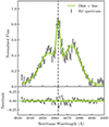 |
Fig. 8. Modeling of the triple-peaked Hβ line with a narrow Gaussian plus the E95 elliptical disk model. The green band shows the best-fit model, and the vertical dashed line corresponds to the rest-frame centroid of Hβ. |
6. Discussion
We have presented multiwavelength time-evolving properties of the X-ray discovered transient J012026. Based on the nuclear position of the source, and the high X-ray luminosity in the 0.2–2.3 keV band (LX = 3.1 × 1043 ergs/s) alone, the source is most likely associated with an accretion event onto an SMBH. Furthermore, the soft X-ray spectrum, the multiwavelength flares (in the MIR and X-ray bands), the He II, and Bowen fluorescence lines observed in the follow-up optical spectra, together with the absence of evidence of previous AGN activity point toward a TDE origin (see, e.g., van Velzen et al. 2020; Saxton et al. 2020; Gezari 2021; Jiang et al. 2021; van Velzen et al. 2021b). However, the erratic X-ray behavior and the relatively narrow profiles of Balmer lines seem to contradict this interpretation. This renders, effectively, J012026 a member of the agnostic ambiguous nuclear transient classification (e.g., Hinkle et al. 2022). In the following section, we further discuss the phenomenological properties and the physical nature of J012026.
6.1. J012026 is a BFF and an ECLE
J012026 shares several properties with the transient class of Bowen fluorescence flares. These events might appear at first glance similar to TDEs, especially due to the presence of transient He II and Bowen fluorescence lines such as N III, which are not to be expected in AGN (Netzer & Peterson 1997). However, BFFs are different from standard TDEs as their overall photometric evolution is slower (a few years rather than a few months), and the transient emission lines are narrower (a few 103 km s−1 rather than a few 104 km s−1) and more persistent than in TDEs (e.g., Trakhtenbrot et al. 2019; Makrygianni et al. 2023).
Indeed, the X-ray, optical, and MIR flares of J01206 evolved over a timescale of about 1000 days, on the longer end of typical optically selected TDEs (e.g., van Velzen et al. 2020; Saxton et al. 2020; Jiang et al. 2021; van Velzen et al. 2021b), although we note that MIR flares of similar profiles have been used to select infrared populations of TDEs (Masterson et al. 2024). Moreover, both Balmer and He II+N III lines detected in the spectra of J012026 have FWHM < 3000 km s−1 and persist for > 600 days, compatible with typical BFF spectral properties. The Balmer lines, in particular, are detected up to four years after the initial discovery.
An additional feature that J012026 shares with BFFs is the presence of coronal lines. Indeed, Most sources of the same category were also found to emit strong and, in some cases, extreme coronal lines. This is the case for F01004-2237 (Tadhunter et al. 2017), AT 2021loi (Makrygianni et al. 2023), AT 2019avd Malyali et al. 2021), AT 2017bgt (Trakhtenbrot et al. 2019), AT 2022fxp Koljonen et al. 2024), AT 2019aalc (Veres et al. 2024; Ŝniegowska et al. 2025), and AT 2019pev (Frederick et al. 2021). As discussed in Sect. 5, the coronal lines [Fe X] and [Fe XIV](+[Fe VII]) are strongly detected in the follow-up spectra of J012026. Interestingly, they have comparable intensity to [O III] 5007, making J012026 also part of the ECLE class. Following the discussion in Veres et al. (2024), which also reports a nuclear transient associated with both the BFF and ECLE class, we confirm the connection between ECLEs and strong MIR flares. This supports the scenario proposed in Wang et al. (2012), and observationally supported for the first time by the work of Onori et al. (2022), in which coronal lines arise due to dust-rich environments being sublimated by TDE-like flares and exposing iron atoms to the ionizing field.
A summary and visual representation of the spectroscopic similarities and differences between J012026, TDEs, BFFs, and ECLEs, can be seen in Fig. 9. In the figure, the spectrum of J012026 is compared with the example spectra of the other discussed classes of transients. The similarities between J012026 with BFFs and coronal line TDEs appear stronger than with the typical Bowen TDE case (AT 2019dsg, AT 2018dyb, and iPTF15af, respectively; van Velzen et al. 2021a; Leloudas et al. 2019; Blagorodnova et al. 2019). However, we note that for two Bowen TDEs (ASASSN-14li and AT 2022wtn, respectively Holoien et al. 2016; Onori et al. 2025), at least in one epoch, the emission line profile of the He II and N III complex appeared narrow and resolved, resembling that of BFFs, and possibly hinting at a connection between these classes.
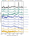 |
Fig. 9. Comparison of spectrum 3 of J012026 with examples of the different transient classes discussed transients: BFFs (In green, AT 2021loi; Makrygianni et al. 2023, AT 2019avd; Malyali et al. 2023a; Frederick et al. 2021, and AT 2022fpx; Koljonen et al. 2024), TDEs with Bowen features (in blue, ASASSN-14li; Holoien et al. 2016, AT 2022wtn; Onori et al. 2025, AT 2019dsg; van Velzen et al. 2021a, AT 2018dyb; Leloudas et al. 2019, and iPTF15af, Blagorodnova et al. 2019), and TDEs with coronal lines (in yellow, AT 2017gge, Onori et al. 2022, and AT 2022upj, Newsome et al. 2024). The gray-shaded areas show, respectively from left to right, the wavelength corresponding to Hδ, Hγ, N III, He III, Hβ and [O III]λ5007. The presented spectra are retrieved from the transient name server or from the ESO archive. |
J012026, however, presents several unique features with respect to the aforementioned classes. Indeed, BFFs are characterized by late-time re-brightenings in their optical light curves (e.g., Koljonen et al. 2024). In the case of J012026, we do not have evidence of such a re-brightening in the optical light curve. However, we do observe such a feature in the X-rays, on timescales of both a few hours and a few months (Fig. 3). In fact, the eRASS5 re-brightening brings the baseline flux back to its discovery eRASS2 level for at least one day. The separation between the peaks cannot be constrained accurately, but it is between one and two years. This is similar to the 1-year timescale observed in the optical light curves of AT 2022fpx and AT 2021loi, and possibly AT 2019pev (Koljonen et al. 2024; Makrygianni et al. 2023; Frederick et al. 2021), and to the X-ray behavior of AT 2019aalc (Veres et al. 2024; Ŝniegowska et al. 2025). The similarity of the timescales could be connected to the inferred SMBH masses, which are on the order of MSMBH ∼ 107 M⊙ for all of the mentioned sources. Koljonen et al. 2024 notes that the differences between the amplitude of the optical re-brightening in AT 2022fpx (lower) and AT 2021loi (higher) and an X-ray re-brightening being only confidently detected in AT 2022fpx could be ascribed to the presence of larger amounts of circumnuclear material reprocessing the primary accretion-powered X-ray emission into optical wavelengths. In a scenario in which BFFs are powered by TDEs reactivating dormant AGN, the unique long-term X-ray light curve of J012026 would fit in the picture as an event observed nearly face-on, where we expect the X-ray emission to be the strongest and to experience little reprocessing along the line of sight (Dai et al. 2018). The orientation claim is supported by the presence of strong Fe II (Charalampopoulos et al. 2022) and by the inclination inferred by modeling the disk lines in spectrum 5 (see Sect. 5.4). However, we note that the physical origin of the re-brightening has yet to be clarified.
In Sect. 5 we have highlighted how the Balmer and He I lines are systematically shifted toward the red, with respect to the higher-ionization lines. We suggest that this evidence points toward the contribution to the lines coming from different kinematical components of the transient, as also argued for some TDEs, such as AT 2022wtn (Onori et al. 2025). In fact, He II, N III, and the coronal lines are likely to originate around the X-ray emitting accretion disk due to the required high-ionization radiation field. Instead, the Balmer lines seem to receive a significant contribution from an asymmetrical, nonspherical outflow, which, due to our line of sight, makes them appear receding. One possible origin of this receding material, in the case of TDEs, is a collision-induced outflow (CIO; Lu & Bonnerot 2020; Jiang et al. 2016), happening at the self-intersection point, which is naturally nonspherical. In this context, the Balmer lines also appear reddened in the latest spectrum, either due to self-absorption or because of the cooling down of the nuclear material after the event is terminated.
We note, however, that in the rejuvenated SMBH interpretation of BFFs, the Balmer, He II, and N III lines are all produced in a preexisting BLR-like structure. The observed dynamical decoupling of these components in J012026, shown by both the width and different shifts of the lines, adds complexity to the physical interpretation of BFFs. This is also the case for the puzzling appearance of the triple-peaked Hβ in spectrum 5, although we suggest that a local obscuration event could temporarily suppress the main emission component and expose the weaker, underlying disk emission in that epoch.
6.2. The short-time X-ray variability
As mentioned in Sect. 2, J012026 caught our attention not only as a TDE, but also because it triggered the QPE detection pipeline developed in Arcodia et al. (2024), which is based on the detection of significant eROday variability. Indeed, the eRASS3 and eRASS5 light curves show variability on eROday timescales, and the second and third Swift/XRT observations have also detected high flux states comparable to the total eRASS2 or eRASS3 and eRASS5 flare fluxes. The Swift/XRT snapshots are on the order of 1 ks; therefore, the flaring timescales are possibly similar to what is observed in the eROSITA light curves (40 s). Additionally, we see a tentative harder-when-brighter behavior, consistent with the QPE spectral evolution as shown in Fig. 4, and discussed in Sect. 3.
The two flares in eRASS5 are separated by 16 hours each. Our longest observation with XMM-Newton covers a baseline of 12 hours, making it possible that, if the flares are due to QPEs with a period of 16 hours, our observation fell right in the quiescence period and missed any new flare. The latest Swift/XRT observations, however, which last 400s, with a cadence of 1-2 hours over a total baseline of three days, also resulted in non-detections. Therefore, if the source is indeed emitting QPEs: (1) the amplitude of the peaks is below the Swift/XRT upper limits, (2) the period is longer than expected, (3) the period is very irregular (see, e.g., ZTF19acnskyy; Hernández-García et al. 2025), or (4) the source is experiencing a quiet phase, similarly to what has been observed for GSN069 (Miniutti et al. 2019). While all of these possibilities are feasible, and we encourage further X-ray follow-up of this source, we note that the evidence pointing toward the variability of J012026 being due to QPEs is as yet tentative despite our dedicated follow-up programs. Therefore, we explore other models that could explain the short-timescale flares.
One possible scenario explaining the X-ray variability is supported by the disk orientation suggested by the triple-peaked Hβ and by the X-ray brightness of the event. In such a configuration, the line of sight could intercept the inner regions of the accretion disk with little to no reprocessing material to smooth out any accretion flow-driven variability. Indeed, accretion flows are known to be variable on timescales spanning several orders of magnitude (e.g., Ulrich et al. 1997; Czerny 2004). In the case of J012026, the observed shortest timescale of X-ray variability is 16 hours eRASS4, which is fully consistent with the thermal timescale at 3–10 Rg for a 107 M⊙ SMBH, assuming an α-disk with α = 0.1 (Czerny 2004). Therefore, thermal fluctuations in the innermost regions of the accretion disk could potentially explain the erratic X-ray behavior, although the amplitude of the variability is quite extreme.
Alternatively, another scenario that could give rise to short-time X-ray variability can be connected to the high-density environment in which the TDE is expected to be taking place, as suggested by the MIR flare, the coronal lines, and the BFF classification. The simulations of Ryu et al. (2024) of TDEs in AGNs have revealed that a star’s passage inside a disk will perturb it and cause instabilities. Even though their analysis focused on the TDE debris, it was observed that these perturbations can cause the disk gas to rain down onto the SMBH. We speculate that these episodic accretion events could superimpose on the TDE light curve and cause short-time X-ray variability on free-fall timescales. In this scenario, in order for the flares to be present in eRASS3, SWIFT-XRT3, SWIFT-XRT4 and eRASS5, perturbations to the disk need to reoccur every ∼5 months. This would in principle be feasible if the disrupted star was on a bound orbit, and the TDE was not full, but rather partial (pTDE; e.g., Liu et al. 2023, 2024). We note, however, that our observations generally do not show any evidence supporting a pTDE scenario, although currently, no numerical work on the emission signatures of pTDE in high-density environments or AGN disks exists, to our knowledge. Overall, the extreme multi-scale X-ray variability of J012026 remains puzzling, and further theoretical work is needed. This is especially crucial if the origin of the X-ray re-brightenings in J012026 is connected to the opticalre-brightenings in other members of the BFF class.
7. Summary and conclusions
We have presented multiwavelength observations of the unique nuclear transient J012026. We summarize the main results as follows:
-
J012026 was discovered as a bright (F0.2 − 2.3 = 1.14 × 10⁻¹² erg/s/cm2) and soft (Γ = 4.3) nuclear X-ray transient in eRASS2. Subsequent eRASS scans and follow-up observations confirmed the transient nature of the source and revealed X-ray variability both on hour and month timescales.
-
The multiwavelength light curves from ATLAS and WISE revealed the presence of long-lived flares (∼2 years). The MIR flare has an amplitude of 0.5–0.7 mag, while the optical flare is less constrained and with evidence of a flux increase > 3 year prior to the X-ray discovery.
-
Follow-up optical spectroscopy revealed a richness of transient features not detected in the archival spectrum, namely (1) redshifted Balmer lines with FWHMs of ∼1500 km s−1, lasting for over four years, (2) He II and the Bowen N III line with FWHMs of ∼2000 km s−1, (4) strong Fe II, (5) high-ionization coronal lines ([Fe X],[Fe XIV], and possibly [Fe VII]), and (6) a triple-peaked Hβ line in one spectrum, suggesting an origin from an elliptical disk-like structure.
-
The optical spectral features, along with the long duration of the event and the strong MIR flare, make this object part of the BFF and ECLE classes. Optical re-brightenings are common among BFFs, yet J012026 shows this feature only in the X-rays, unlike any other source of this class. The re-brightening timescales and black hole masses are also compatible with events AT 2021loi and AT 2022fpx. In the interpretation in which BFFs are TDEs that are rejuvenating AGN, J012026 would represent a face-on event based on the X-ray to optical properties and optical spectral features.
-
We discussed possible models to explain the short- and long-term X-ray variability; however, the question is still unresolved. We stress the need for more theoretical predictions of the X-ray properties of full TDEs and pTDEs in high-density environments (such as AGN disks).
J012026, overall, shows a complex interplay of features, bridging the classification of nuclear transients of TDEs, ECLEs, BFFs, and ambiguous nuclear transients. The richness in multiwavelength features points toward an ambiguous origin of the transient, and more theoretical and observational work is encouraged to narrow down the physical origin of analogous sources. We highlight that, without the early X-ray detection, this source would not have been selected as optically variable. This is testimony to the importance of X-ray time-domain surveys, such as eROSITA and EP, for gaining a full picture of nuclear transients.
Acknowledgments
PB is grateful for the insightful discussions with Megan Newsome, Paola Martire, and Fabian Balzer about the work. This work is based on data from eROSITA, the soft X-ray instrument aboard SRG, a joint Russian-German science mission supported by the Russian Space Agency (Roscosmos), in the interests of the Russian Academy of Sciences represented by its Space Research Institute (IKI), and the Deutsches Zentrum für Luft- und Raumfahrt (DLR). The SRG spacecraft was built by Lavochkin Association (NPOL) and its subcontractors, and is operated by NPOL with support from the Max Planck Institute for Extraterrestrial Physics (MPE). The development and construction of the eROSITA X-ray instrument was led by MPE, with contributions from the Dr. Karl Remeis Observatory Bamberg & ECAP (FAU Erlangen-Nuernberg), The University of Hamburg Observatory, the Leibniz Institute for Astrophysics Potsdam (AIP), and the Institute for Astronomy and Astrophysics of the University of Tübingen, with the support of DLR and the Max Planck Society. The Argelander Institute for Astronomy of the University of Bonn and the Ludwig Maximilians Universität Munich also participated in the science preparation for eROSITA. The eROSITA data shown here were processed using the eSASS software system developed by the German eROSITA consortium. Some of the observations reported in this paper were obtained with the Southern African Large Telescope (SALT), as part of the Large Science Programme on transients 2018-2-LSP-001 (PI: Buckley). This work is based on data obtained with the Einstein Probe, a space mission supported by the Strategic Priority Program on Space Science of the Chinese Academy of Sciences, in collaboration with ESA, MPE and CNES (Grant No. XDA15310000, No. XDA15052100). R.A. was supported by NASA through the NASA Hubble Fellowship grant #HST-HF2-51499.001-A awarded by the Space Telescope Science Institute, which is operated by the Association of Universities for Research in Astronomy, Incorporated, under NASA contract NAS5-26555. M.K. is supported by DLR grant FKZ 50 OR 2307. This work was supported by the Australian government through the Australian Research Council’s Discovery Projects funding scheme (DP200102471) The Australia Telescope Compact Array is part of the Australia Telescope National Facility (grid.421683.a) which is funded by the Australian Government for operation as a National Facility managed by CSIRO. This work has made use of data from the Asteroid Terrestrial-impact Last Alert System (ATLAS) project. The Asteroid Terrestrial-impact Last Alert System (ATLAS) project is primarily funded to search for near earth asteroids through NASA grants NN12AR55G, 80NSSC18K0284, and 80NSSC18K1575; byproducts of the NEO search include images and catalogs from the survey area. This work was partially funded by Kepler/K2 grant J1944/80NSSC19K0112 and HST GO-15889, and STFC grants ST/T000198/1 and ST/S006109/1. The ATLAS science products have been made possible through the contributions of the University of Hawaii Institute for Astronomy, the Queen’s University Belfast, the Space Telescope Science Institute, the South African Astronomical Observatory, and The Millennium Institute of Astrophysics (MAS), Chile.
References
- Arcavi, I., Gal-Yam, A., Sullivan, M., et al. 2014, ApJ, 793, 38 [Google Scholar]
- Arcodia, R., Merloni, A., Nandra, K., et al. 2021, Nature, 592, 704 [NASA ADS] [CrossRef] [Google Scholar]
- Arcodia, R., Merloni, A., Buchner, J., et al. 2024, A&A, 684, L14 [NASA ADS] [CrossRef] [EDP Sciences] [Google Scholar]
- Assef, R. J., Stern, D., Kochanek, C. S., et al. 2013, ApJ, 772, 26 [Google Scholar]
- Bellm, E. C., Kulkarni, S. R., Graham, M. J., et al. 2018, PASP, 131, 018002 [Google Scholar]
- Bianchi, L., Shiao, B., & Thilker, D. 2017, Ap&SS, 230, 24 [Google Scholar]
- Blagorodnova, N., Cenko, S. B., Kulkarni, S. R., et al. 2019, ApJ, 873, 92 [NASA ADS] [CrossRef] [Google Scholar]
- Boller, T., Freyberg, M., Trümper, J., et al. 2016, A&A, 588, A103 [NASA ADS] [CrossRef] [EDP Sciences] [Google Scholar]
- Bonnerot, C., Rossi, E. M., & Lodato, G. 2017, MNRAS, 464, 2816 [Google Scholar]
- Bowen, I. S. 1928, ApJ, 67, 1 [Google Scholar]
- Brunner, H., Liu, T., Lamer, G., et al. 2022, A&A, 661, A1 [NASA ADS] [CrossRef] [EDP Sciences] [Google Scholar]
- Buchner, J. 2019, PASP, 131, 108005 [Google Scholar]
- Buchner, J. 2021, JOSS, 6, 3001 [NASA ADS] [CrossRef] [Google Scholar]
- Buchner, J., Georgakakis, A., Nandra, K., et al. 2014, A&A, 564, A125 [NASA ADS] [CrossRef] [EDP Sciences] [Google Scholar]
- Buchner, J., Boller, T., Bogensberger, D., et al. 2022, A&A, 661, A18 [NASA ADS] [CrossRef] [EDP Sciences] [Google Scholar]
- Buchner, J., Starck, H., Salvato, M., et al. 2024, A&A, 692, A161 [NASA ADS] [CrossRef] [EDP Sciences] [Google Scholar]
- Buckley, D. A., Andreoni, I., Barway, S., et al. 2018, MNRAS, 474, L71 [NASA ADS] [CrossRef] [Google Scholar]
- Buckley, D. A., Swart, G. P., & Meiring, J. G. 2006, in Ground-based and Airborne Telescopes, SPIE, 6267, 333 [Google Scholar]
- Burgh, E. B., Nordsieck, K. H., Kobulnicky, H. A., et al. 2003, in Instrument Design and Performance for Optical/Infrared Ground-based Telescopes, SPIE, 4841, 1463 [NASA ADS] [CrossRef] [Google Scholar]
- Buzzoni, B., Delabre, B., Dekker, H., et al. 1984, Msngr, 38, 9 [Google Scholar]
- Cappellari, M. 2023, MNRAS, 526, 3273 [NASA ADS] [CrossRef] [Google Scholar]
- CASA Team (Bean, B., et al.) 2022, PASP, 134, 114501 [NASA ADS] [CrossRef] [Google Scholar]
- Cerqueira-Campos, F., Rodríguez-Ardila, A., Riffel, R., et al. 2021, MNRAS, 500, 2666 [Google Scholar]
- Chambers, K. C., Magnier, E. A., Metcalfe, N., et al. 2016, ArXiv e-prints [arXiv:1612.05560] [Google Scholar]
- Charalampopoulos, P., Leloudas, G., Malesani, D. B., et al. 2022, A&A, 659, A34 [NASA ADS] [CrossRef] [EDP Sciences] [Google Scholar]
- Childress, M. J., Vogt, F. P. A., Nielsen, J., & Sharp, R. G. 2014, Ap&SS, 349, 617 [Google Scholar]
- Colless, M., Dalton, G., Maddox, S., et al. 2001, MNRAS, 328, 1039 [Google Scholar]
- Conroy, C., & Gunn, J. E. 2010, Astrophysics Source Code Library [record ascl:1010.043] [Google Scholar]
- Crawford, S. M., Still, M., Schellart, P., et al. 2010, in Observatory Operations: Strategies, Processes, and Systems III, SPIE, 7737, 550 [Google Scholar]
- Czerny, B. 2004, ArXiv e-prints [arXiv:astro-ph/0409254] [Google Scholar]
- Dai, L., McKinney, J. C., Roth, N., Ramirez-Ruiz, E., & Miller, M. C. 2018, ApJ, 859, L20 [Google Scholar]
- Dey, A., Schlegel, D. J., Lang, D., et al. 2019, AJ, 157, 168 [Google Scholar]
- Dopita, M., Rhee, J., Farage, C., et al. 2010, Ap&SS, 327, 245 [Google Scholar]
- Earl, N., French, K. D., Ramirez-Ruiz, E., et al. 2025, ApJ, 983, 28 [Google Scholar]
- Eracleous, M., Livio, M., Halpern, J. P., & Storchi-Bergmann, T. 1995, ApJ, 438, 610 [NASA ADS] [CrossRef] [Google Scholar]
- Evans, C. R., & Kochanek, C. S. 1989, ApJ, 346, L13 [Google Scholar]
- Evans, P., Beardmore, A. P., Page, K. L., et al. 2007, A&A, 469, 379 [NASA ADS] [CrossRef] [EDP Sciences] [Google Scholar]
- Evans, P., Beardmore, A., Page, K., et al. 2009, MNRAS, 397, 1177 [NASA ADS] [CrossRef] [Google Scholar]
- Frederick, S., Gezari, S., Graham, M. J., et al. 2021, ApJ, 920, 56 [NASA ADS] [CrossRef] [Google Scholar]
- Freudling, W., Romaniello, M., Bramich, D. M., et al. 2013, A&A, 559, A96 [NASA ADS] [CrossRef] [EDP Sciences] [Google Scholar]
- Fruscione, A., McDowell, J. C., Allen, G. E., et al. 2006, in Observatory Operations: Strategies, Processes, and Systems, eds. D. R. Silva, & R. E. Doxsey, SPIE Conf. Ser., 6270, 62701V [NASA ADS] [CrossRef] [Google Scholar]
- Gabriel, C., Denby, M., Fyfe, D., et al. 2004, Astronomical Data Analysis Software and Systems (ADASS) XIII, 314, 759 [NASA ADS] [Google Scholar]
- Gehrels, N., Chincarini, G., Giommi, P., et al. 2004, ApJ, 611, 1005 [Google Scholar]
- Gezari, S. 2021, ARA&A, 59, 21 [NASA ADS] [CrossRef] [Google Scholar]
- Gezari, S., Chornock, R., Rest, A., et al. 2012, Nature, 485, 217 [Google Scholar]
- Giustini, M., Miniutti, G., & Saxton, R. D. 2020, A&A, 636, L2 [NASA ADS] [CrossRef] [EDP Sciences] [Google Scholar]
- Greiner, J., Schwarz, R., Zharikov, S., & Orio, M. 2000, A&A, 362, L25 [NASA ADS] [Google Scholar]
- Grotova, I., Rau, A., Salvato, M., et al. 2025a, A&A, 693, A62 [NASA ADS] [CrossRef] [EDP Sciences] [Google Scholar]
- Grotova, I., Rau, A., Baldini, P., et al. 2025b, A&A, 697, A159 [NASA ADS] [CrossRef] [EDP Sciences] [Google Scholar]
- Grupe, D., Thomas, H. C., & Leighly, K. M. 1999, A&A, 350, L31 [NASA ADS] [Google Scholar]
- Guillochon, J., Manukian, H., & Ramirez-Ruiz, E. 2014, ApJ, 783, 23 [NASA ADS] [CrossRef] [Google Scholar]
- Guo, H., Sun, J., Li, S., et al. 2025, ApJ, 979, 235 [Google Scholar]
- Guolo, M., Gezari, S., Yao, Y., et al. 2024a, ApJ, 966, 160 [NASA ADS] [CrossRef] [Google Scholar]
- Guolo, M., Pasham, D. R., Zajaček, M., et al. 2024b, Nat. Astron., 8, 347 [Google Scholar]
- Hernández-García, L., Chakraborty, J., Sánchez-Sáez, P., et al. 2025, Nat. Astron., 9, 895 [Google Scholar]
- HI4PI Collaboration (Ben Bekhti, N., et al.) 2016, A&A, 594, A116 [NASA ADS] [CrossRef] [EDP Sciences] [Google Scholar]
- Hills, J. G. 1975, Nature, 254, 295 [Google Scholar]
- Hinkle, J. T., Holoien, T. W.-S., Shappee, B. J., et al. 2022, ApJ, 930, 12 [NASA ADS] [CrossRef] [Google Scholar]
- Hinkle, J. T., Shappee, B. J., & Holoien, T. W. S. 2024, MNRAS, 528, 4775 [Google Scholar]
- Holoien, T. W. S., Kochanek, C. S., Prieto, J. L., et al. 2016, MNRAS, 455, 2918 [NASA ADS] [CrossRef] [Google Scholar]
- Holoien, T. W. S., Huber, M. E., Shappee, B. J., et al. 2019, ApJ, 880, 120 [NASA ADS] [CrossRef] [Google Scholar]
- Homan, D., Krumpe, M., Markowitz, A., et al. 2023, A&A, 672, A167 [NASA ADS] [CrossRef] [EDP Sciences] [Google Scholar]
- Hung, T., Cenko, S. B., Roth, N., et al. 2019, ApJ, 879, 119 [NASA ADS] [CrossRef] [Google Scholar]
- Jansen, F., Lumb, D., Altieri, B., et al. 2001, A&A, 365, L1 [NASA ADS] [CrossRef] [EDP Sciences] [Google Scholar]
- Jiang, N., Wang, T., Hu, X., et al. 2021, ApJ, 911, 31 [NASA ADS] [CrossRef] [Google Scholar]
- Jiang, Y.-F., Guillochon, J., & Loeb, A. 2016, ApJ, 830, 125 [NASA ADS] [CrossRef] [Google Scholar]
- Jones, E., Oliphant, T., Peterson, P., et al. 2001, SciPy: Open source scientific tools for Python, http://www.scipy.org/ [Google Scholar]
- Kass, R. E., & Raftery, A. E. 1995, Journal of the Am. Stat. Assoc., 90, 773 [Google Scholar]
- Khorunzhev, G., Sazonov, S. Y., Medvedev, P., et al. 2022, AstL, 48, 767 [Google Scholar]
- Kochanek, C., Shappee, B., Stanek, K., et al. 2017, PASP, 129, 104502 [NASA ADS] [CrossRef] [Google Scholar]
- Koljonen, K. I. I., Liodakis, I., Lindfors, E., et al. 2024, MNRAS, 532, 112 [Google Scholar]
- Komossa, S. 2015, JHEAp, 7, 148 [NASA ADS] [Google Scholar]
- Komossa, S., & Bade, N. 1999, in Highlights in X-ray Astronomy, eds. B. Aschenbach, & M. J. Freyberg, 272, 143 [Google Scholar]
- Komossa, S., & Greiner, J. 1999, A&A, 349, L45 [NASA ADS] [Google Scholar]
- Komossa, S., Zhou, H., Wang, T., et al. 2008, ApJ, 678, L13 [NASA ADS] [CrossRef] [Google Scholar]
- Kulkarni, S. R. 2013, ATel, 4807, 1 [NASA ADS] [Google Scholar]
- Law, N. M., Kulkarni, S. R., Dekany, R. G., et al. 2009, PASP, 121, 1395 [NASA ADS] [CrossRef] [Google Scholar]
- Leloudas, G., Dai, L., Arcavi, I., et al. 2019, ApJ, 887, 218 [NASA ADS] [CrossRef] [Google Scholar]
- Lewis, I. J., Cannon, R. D., Taylor, K., et al. 2002, MNRAS, 333, 279 [NASA ADS] [CrossRef] [Google Scholar]
- Liu, T., Buchner, J., Nandra, K., et al. 2022, A&A, 661, A5 [NASA ADS] [CrossRef] [EDP Sciences] [Google Scholar]
- Liu, Z., Malyali, A., Krumpe, M., et al. 2023, A&A, 669, A75 [NASA ADS] [CrossRef] [EDP Sciences] [Google Scholar]
- Liu, Z., Ryu, T., Goodwin, A., et al. 2024, A&A, 683, L13 [NASA ADS] [CrossRef] [EDP Sciences] [Google Scholar]
- Lu, W., & Bonnerot, C. 2020, MNRAS, 492, 686 [NASA ADS] [CrossRef] [Google Scholar]
- Mainzer, A., Bauer, J., Cutri, R. M., et al. 2014, ApJ, 792, 30 [Google Scholar]
- Makrygianni, L., Trakhtenbrot, B., Arcavi, I., et al. 2023, ApJ, 953, 32 [NASA ADS] [CrossRef] [Google Scholar]
- Malyali, A., Rau, A., Merloni, A., et al. 2021, A&A, 647, A9 [NASA ADS] [CrossRef] [EDP Sciences] [Google Scholar]
- Malyali, A., Liu, Z., Merloni, A., et al. 2023a, MNRAS, 520, 4209 [NASA ADS] [CrossRef] [Google Scholar]
- Malyali, A., Liu, Z., Rau, A., et al. 2023b, MNRAS, 520, 3549 [NASA ADS] [CrossRef] [Google Scholar]
- Malyali, A., Rau, A., Bonnerot, C., et al. 2024, MNRAS, 531, 1256 [NASA ADS] [CrossRef] [Google Scholar]
- Marshall, J. L., Burles, S., Thompson, I. B., et al. 2008, in Ground-based and Airborne Instrumentation for Astronomy II, eds. I. S. McLean, & M. M. Casali, SPIE, 7014, 701454 [NASA ADS] [Google Scholar]
- Masterson, M., De, K., Panagiotou, C., et al. 2024, ApJ, 961, 211 [NASA ADS] [CrossRef] [Google Scholar]
- Merloni, A., Lamer, G., Liu, T., et al. 2024, A&A, 682, A34 [NASA ADS] [CrossRef] [EDP Sciences] [Google Scholar]
- Metzger, B. D., & Stone, N. C. 2016, MNRAS, 461, 948 [NASA ADS] [CrossRef] [Google Scholar]
- Miniutti, G., Saxton, R. D., Giustini, M., et al. 2019, Nature, 573, 381 [Google Scholar]
- Negus, J., Comerford, J. M., Sánchez, F. M., et al. 2021, ApJ, 920, 62 [NASA ADS] [CrossRef] [Google Scholar]
- Netzer, H., & Peterson, B. M. 1997, in Astronomical Time Series, eds. D. Maoz, A. Sternberg, & E. M. Leibowitz, Astrophysics and Space Science Library, 218, 85 [Google Scholar]
- Newsome, M., Arcavi, I., Howell, D. A., et al. 2024, ApJ, 977, 258 [Google Scholar]
- Newville, M., Stensitzki, T., Allen, D. B., et al. 2016, Astrophysics Source Code Library [record ascl:1606.014] [Google Scholar]
- Ochmann, M. W., Kollatschny, W., Probst, M. A., et al. 2024, A&A, 686, A17 [NASA ADS] [CrossRef] [EDP Sciences] [Google Scholar]
- Onori, F., Cannizzaro, G., Jonker, P. G., et al. 2019, MNRAS, 489, 1463 [CrossRef] [Google Scholar]
- Onori, F., Cannizzaro, G., Jonker, P., et al. 2022, MNRAS, 517, 76 [NASA ADS] [CrossRef] [Google Scholar]
- Onori, F., Nicholl, M., Ramsden, P., et al. 2025, MNRAS, 540, 498 [Google Scholar]
- Osterbrock, D. E. 1989, Astrophysics of Gaseous Nebulae and Active Galactic Nuclei (University Science Books) [Google Scholar]
- Park, D., Barth, A. J., Ho, L. C., & Laor, A. 2022, Ap&SS, 258, 38 [Google Scholar]
- Parkinson, E. J., Knigge, C., Matthews, J. H., et al. 2022, MNRAS, 510, 5426 [Google Scholar]
- Pasham, D. R., Strohmayer, T. E., & Mushotzky, R. F. 2014, Nature, 513, 74 [Google Scholar]
- Phinney, E. S. 1989, in The Center of the Galaxy, ed. M. Morris, IAU Symposium, 136, 543 [NASA ADS] [CrossRef] [Google Scholar]
- Piran, T., Svirski, G., Krolik, J., Cheng, R. M., & Shiokawa, H. 2015, ApJ, 806, 164 [Google Scholar]
- Planck Collaboration XIII. 2016, A&A, 594, A13 [NASA ADS] [CrossRef] [EDP Sciences] [Google Scholar]
- Predehl, P., Andritschke, R., Arefiev, V., et al. 2021, A&A, 647, A1 [EDP Sciences] [Google Scholar]
- Prieto, A., Rodríguez-Ardila, A., Panda, S., & Marinello, M. 2022, MNRAS, 510, 1010 [Google Scholar]
- Prochaska, J., Hennawi, J., Westfall, K., et al. 2020, JOSS, 5, 2308 [NASA ADS] [CrossRef] [Google Scholar]
- Rees, M. J. 1988, Nature, 333, 523 [Google Scholar]
- Reines, A. E., & Volonteri, M. 2015, ApJ, 813, 82 [NASA ADS] [CrossRef] [Google Scholar]
- Reis, R., Miller, J., Reynolds, M., et al. 2012, Science, 337, 949 [NASA ADS] [CrossRef] [Google Scholar]
- Roth, N., Kasen, D., Guillochon, J., & Ramirez-Ruiz, E. 2016, ApJ, 827, 3 [Google Scholar]
- Ryu, T., Krolik, J., Piran, T., Noble, S. C., & Avara, M. 2023, ApJ, 957, 12 [Google Scholar]
- Ryu, T., McKernan, B., Ford, K. E. S., et al. 2024, MNRAS, 527, 8103 [Google Scholar]
- Saxton, R., Komossa, S., Auchettl, K., & Jonker, P. G. 2020, Space Sci. Rev., 216, 85 [NASA ADS] [CrossRef] [Google Scholar]
- Sazonov, S., Gilfanov, M., Medvedev, P., et al. 2021, MNRAS, 508, 3820 [NASA ADS] [CrossRef] [Google Scholar]
- Schlafly, E. F., & Finkbeiner, D. P. 2011, ApJ, 737, 103 [Google Scholar]
- Shappee, B. J., Prieto, J., Grupe, D., et al. 2014, ApJ, 788, 48 [NASA ADS] [CrossRef] [Google Scholar]
- Shingles, L., Smith, K., Young, D., et al. 2021, TNSAN, 7, 1 [NASA ADS] [Google Scholar]
- Shiokawa, H., Krolik, J. H., Cheng, R. M., Piran, T., & Noble, S. C. 2015, ApJ, 804, 85 [Google Scholar]
- Short, P., Nicholl, M., Lawrence, A., et al. 2020, MNRAS, 498, 4119 [NASA ADS] [CrossRef] [Google Scholar]
- Short, P., Lawrence, A., Nicholl, M., et al. 2023, MNRAS, 525, 1568 [NASA ADS] [CrossRef] [Google Scholar]
- Simmonds, C., Buchner, J., Salvato, M., Hsu, L. T., & Bauer, F. E. 2018, A&A, 618, A66 [NASA ADS] [CrossRef] [EDP Sciences] [Google Scholar]
- Smith, K., Smartt, S., Young, D., et al. 2020, PASP, 132, 085002 [Google Scholar]
- Ŝniegowska, M., Trakhtenbrot, B., Makrygianni, L., et al. 2025, ApJ, submitted [arXiv:2505.00083] [Google Scholar]
- Steinberg, E., & Stone, N. C. 2024, Nature, 625, 463 [NASA ADS] [CrossRef] [Google Scholar]
- Stern, D., Assef, R. J., Benford, D. J., et al. 2012, ApJ, 753, 30 [Google Scholar]
- Stone, N. C., & Metzger, B. D. 2016, MNRAS, 455, 859 [NASA ADS] [CrossRef] [Google Scholar]
- Strüder, L., Briel, U., Dennerl, K., et al. 2001, A&A, 365, L18 [Google Scholar]
- Sunyaev, R., Arefiev, V., Babyshkin, V., et al. 2021, A&A, 656, A132 [NASA ADS] [CrossRef] [EDP Sciences] [Google Scholar]
- Tadhunter, C., Spence, R., Rose, M., Mullaney, J., & Crowther, P. 2017, Nat. Astron., 1, 0061 [NASA ADS] [CrossRef] [Google Scholar]
- Tody, D. 1986, in Instrumentation in Astronomy VI, ed. D. L. Crawford, SPIE Conf. Ser., 627, 733 [NASA ADS] [CrossRef] [Google Scholar]
- Tonry, J., Denneau, L., Heinze, A., et al. 2018, PASP, 130, 064505 [NASA ADS] [CrossRef] [Google Scholar]
- Trakhtenbrot, B., Arcavi, I., Ricci, C., et al. 2019, Nat. Astron., 3, 242 [Google Scholar]
- Trümper, J. 1982, AdSpR, 2, 241 [Google Scholar]
- Tubín-Arenas, D., Krumpe, M., Lamer, G., et al. 2024, A&A, 682, A35 [NASA ADS] [CrossRef] [EDP Sciences] [Google Scholar]
- Turner, M. J., Abbey, A., Arnaud, M., et al. 2001, A&A, 365, L27 [CrossRef] [EDP Sciences] [Google Scholar]
- Ulrich, M.-H., Maraschi, L., & Urry, C. M. 1997, ARA&A, 35, 445 [NASA ADS] [CrossRef] [Google Scholar]
- van Velzen, S., Gezari, S., Hammerstein, E., et al. 2021a, ApJ, 908, 4 [NASA ADS] [CrossRef] [Google Scholar]
- van Velzen, S., Pasham, D. R., Komossa, S., Yan, L., & Kara, E. A. 2021b, Space Sci. Rev., 217, 63 [NASA ADS] [CrossRef] [Google Scholar]
- van Velzen, S., Holoien, T. W. S., Onori, F., Hung, T., & Arcavi, I. 2020, Space Sci. Rev., 216, 124 [CrossRef] [Google Scholar]
- Veres, P. M., Franckowiak, A., van Velzen, S., et al. 2024, A&A, submitted [arXiv:2408.17419] [Google Scholar]
- Wang, T.-G., Zhou, H.-Y., Komossa, S., et al. 2012, ApJ, 749, 115 [Google Scholar]
- Ward, C., Gezari, S., Nugent, P., et al. 2024, ApJ, 961, 172 [NASA ADS] [CrossRef] [Google Scholar]
- Weisskopf, M. C., Tananbaum, H. D., Van Speybroeck, L. P., & O’Dell, S. L. 2000, X-ray Optics Instruments, and Missions iii, 4012, 2 [Google Scholar]
- Wevers, T., Nicholl, M., Guolo, M., et al. 2022, A&A, 666, A6 [NASA ADS] [CrossRef] [EDP Sciences] [Google Scholar]
- Young, D. R. 2020, https://doi.org/10.5281/zenodo.10978968 [Google Scholar]
- Yuan, W. 2022, 44th COSPAR Scientific Assembly. Held 16–24 July, 44, 1966 [Google Scholar]
- Yuan, W., Dai, L., Feng, H., et al. 2025, Sci. China Phys. Mech. Astron., 68, 239501 [Google Scholar]
Appendix A: Supplementary material on X-ray observations
A.1. Contamination from nearby AGN WISEA J012025-292637
To estimate the possible contamination of WISEA J012025-292637, we extracted light curves at the locations of J012026 and WISEA J012025-292637, in addition to an annulus background region of inner and outer radii of 115" and 160". We used a circular region for J012026 with a radius of 40", corresponding to ∼80% of the encircled energy fraction. For WISEA J012025-292637, we used a region with a radius of 15", which corresponds to ∼50% of the encircled energy fraction. We chose such radii in order to avoid overlapping between the two regions, while still being able to estimate the total number of counts, through our knowledge of the eROSITA point spread function. The extraction regions are shown in Fig. A.1 over the stacked eRASS:5 image. We then computed the fraction f of the remaining 50% photons coming from WISEA J012025-292637 that would fall in the extraction region of J012026, by measuring the angle between the lines tangent to such an extraction region, passing through the WISEA J012025-292637 position.
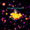 |
Fig. A.1. eRASS:5 image of J012026 and the nearby AGN WISEA J012025-292637. The image had been smoothed for visualization purposes. The white circle represents the extraction region of J012026 used in the procedure to estimate the contamination, and the cyan circle is the region used for WISEA J012025-292637. |
In Fig. A.2 we plot the light curves of J012026 and the maximum expected contamination by WISEA J012025-292637, estimated from the 50% extraction region and corrected by the factor f, respectively, in red circles and blue squares. We conclude that WISEA J012025-292637 was bright only in eRASS1, as also shown by the cutouts in Fig. A.3, and did not contaminate the remaining observations. Therefore, we used pipeline products.
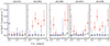 |
Fig. A.2. eROSITA eROday 0.2-2.3 keV band light curve of J012026 (red) and WISEA J012025-292637 (blue) extracted respectively with regions of 15" and 40" in radius. The gray triangles correspond to the background count rate |
A.2. X-ray spectra and analysis of the harder-when-brighter behavior
We show the eRASS2-5, Swift-XRT3, and Swift-XRT4 spectra in Fig. A.4. The figures show both the source and background data and models, both for the DISKBB and power-law fits.
As discussed in Sect. 3, the results of the X-ray spectral fits suggest a general anticorrelation between the X-ray flux and the power-law photon index, Γ. To quantitatively test this hypothesis, we performed a Monte Carlo evaluation of the Pearson correlation coefficient, r, uniformly sampling our dataset accounting for uncertainties in both fluxes and photon indices. The resulting distribution of r is shown in Fig. A.5. The median value of r = −0.56 suggests a possible anticorrelation; however, the 95% confidence interval of the distribution includes zero, indicating that the observed trend is not statistically significant.
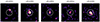 |
Fig. A.3. eROSITA images of J012026. The images have been smoothed for visualization purposes, and the white circle represents a region of 60" in radius. |
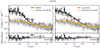 |
Fig. A.4. X-ray spectra of J012026. The observation name is reported in the title. All panels show, respectively with black and gray markers, the source and background counts, which have been re-binned for visualization purposes. The left panels show the DISKBB fit (dashed black line) with 1σ uncertainties (blue band), while the right panels show the same results for the power-law model (black dashed line and pink band). In all panels, the orange line shows the background model. |
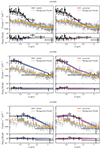 |
Fig. A.4. Continued. |
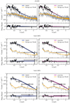 |
Fig. A.4. Continued. |
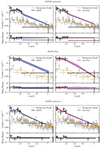 |
Fig. A.4. Continued. |
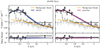 |
Fig. A.4. Continued. |
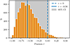 |
Fig. A.5. Distribution of the Pearson correlation coefficient, r. The continuous vertical line indicate the median value of r = −0.56, and the dashed line shows r = 0. The gray-shaded area indicates the 95% confidence interval. |
Appendix B: Radio properties of J012026
To search for any transient radio emission associated with the multiwavelength outburst, we observed the coordinates of J012026 with the ATCA on three occasions in October 2022 (ATCA program C3513), June 2023 (ATCA program C3513), and March 2024 (ATCA program C3586). In the first and third observations, we observed with the dual 5.5 and 9 GHz receiver with 2 GHz of bandwidth split into 2048 spectral channels at each central frequency. In the second observation, we observed with the dual 5.5 and 9 GHz receiver as well as the 2.1 GHz receiver with 2 GHz of bandwidth split into 2048 spectral channels. All observations were taken in the extended 6 km configuration. The observations in October 2022 and March 2024 were approximately 4 hr long, and the observation in June 2023 was approximately 6 hr long. In all observations, PKS 1934–638 was used for flux and bandpass calibration and PKS 0142-278 for phase calibration. All data were reduced using standard procedures in the Common Software Astronomy Application (CASA; CASA Team 2022). Images of the target field were created using the CASA task tclean and target flux density extracted by fitting a Gaussian to the size of the synthesized beam using the CASA task imfit. In all observations except the 5.5 GHz observation on October 3, 2022, and March 25, 2024, no radio source was detected at the coordinates of J012026, with a 3σ upper limit extracted as three times the image rms. In the observations at 5.5 GHz on October 3, 2022, and March 25, 2024, a marginal point source was detected at the location of J012026 with a flux density of 55 ± 9 and 37 ± 6 uJy, i.e., a 6σ detection in each observation. The source was not detected in the 5.5 GHz observation on June 23, 2023. We report the flux density measurements and upper limits in Table B.1.
The two marginal radio detections of J012026 at 5.5 GHz may indicate variable jet activity related to the transient activity in the galaxy, although, without spectral information, it is difficult to determine the nature of the radio emission. However, the detections are marginal and may also be spurious noise peaks in the images.
ATCA radio observations of J012026.
Appendix C: Supplementary material on optical spectroscopy
C.1. The archival spectrum of J012026
We present the archival spectrum of J012026 in Fig. C.1, as retrieved from the NASA/IPAC Extragalactic Database. The spectrum was obtained by the 2dF spectrograph on the Anglo-Australian Telescope (AAT), and has a resolution of Δλ ∼ 9 Å. No evident features are present, with the exception of the Ca H & K doublet.
C.2. Spectral reduction
NTT: The source was observed with the ESO Faint Object Spectrograph and Camera v.2 (EFOSC2; Buzzoni et al. 1984) mounted on the ESO NTT in La Silla, Chile (proposal ID: 108.225J.001, PI Grotova). The grism 13 and the 1.2″slit were used for the observation, providing a wavelength range of 3685−9315 Å with a dispersion of 2.77 Å/pixel. The observations were performed with an airmass of 1.3. The data reduction and calibration were performed with the esoreflex pipeline (Freudling et al. 2013, v2.11.5). For wavelength and flux calibration, we used the He+Ar arcs and a standard star observed with the same grism and slit, oriented along the parallactic angle.
 |
Fig. C.1. Archival 2dF spectrum of the nucleus of J012026. The black vertical lines show the rest-frame wavelengths of the Ca H & K doublet, Hβ, and the [O III] doublet. The spikes slightly redward of the [O III] doublet and around ∼ 5700 Å are likely artifacts. |
MagE: We observed J012026 with the MagE spectrograph (Marshall et al. 2008) mounted on 6.5m Magellan/Baade Telescope as Las Campanas Observatory on 16 December 2023. The total observation duration was 1 hour, with an airmass of 1.06, and the 0.5″slit was used. We reduced the data with pypeit (Prochaska et al. 2020) and followed standard data reduction procedures, including wavelength calibration with ThAr lamps and flux calibration with observations of a nearby standard star on the same night.
WiFeS: We obtained a spectrum of J012026 with the Wide Field Spectrograph (WiFeS; Dopita et al. 2010) mounted on the 2.3m Australian National University (ANU) telescope at Siding Spring Observatory. We used the R3000 and B3000 gratings, providing a resolution of R = 3000 and a spectral coverage of 3500 to 7000 Å. The observations were performed with an airmass of 1.02. The data were reduced using the PyWiFeS reduction pipeline (Childress et al. 2014), which produces three-dimensional data cubes. The spectra in these cubes were bias subtracted, flat-fielded, wavelength (with a NeAr lamp), and flux calibrated (using the flux standard EG 131). Finally, the spectra were extracted from the slitlets that captured J012026 using the IRAF task APALL (Tody 1986), which allowed for background subtraction.
SALT: We obtained SALT spectra on the nights of July 18, 2020, and July 17, 2021, using the RSS (RSS; Burgh et al. 2003; Buckley et al. 2006). For both observations, the airmass was 1.18. We used the PG0900 grating with a 1.25 arcsec slit. The wavelength range is from 4060 to 7110 Åwith a typical resolution of R ∼1200. Observations were reduced using a custom pipeline based on the PySALT package (Crawford et al. 2010), which accounts for basic CCD characteristics (e.g., cross-talk, bias and gain correction), removal of cosmic rays, wavelength calibration, and relative flux calibration. Standard IRAF/Pyraf routines were used to accurately account for sky background removal. Absolute flux calibration with SALT is difficult because of the telescope design, which has a moving, field-dependent and under-filled entrance pupil. Observations of spectrophotometric flux standards can, at best, only provide relative flux calibration (see, e.g., Buckley et al. 2018), which mostly accounts for the low-frequency telescope and instrument sensitivity changes as a function of wavelength.
IMACS and LDSS3-C: For the Baade IMACS observation, we used the long-slit mode with Grism 300-17.5, which covered the range 4254-9454 Å with a dispersion of 1.27 Å/px. In combination with a slit of 0.7″ the instrumental resolution was about 4.7 Å. The total exposure time was 900 sec, the seeing was approximately around 0.8″, and the airmass 1.4. For the Clay LDSS3-C observation, we used the VPH-All grating with a 1″slit. The grating covered the range 3565-10608 Åwith a dispersion of 1.99 /px and a resolution of about 8.3 Å. A total exposure time of 2100 sec was applied under a seeing of about 1.3″, with an airmass of 1.54. In both cases, spectra were reduced with IRAF following the usual procedure of overscan and flat-field correction, wavelength calibration by means of a He-Ne-Ar lamp, and flux calibration through the observation of a spectrophotometric standard star. LTT1788 was observed with IMACS and the same slit used for the target, while LTT2415 was observed with LDSS3-C and a slit of 6″. Finally, the night-sky contribution was subtracted by fitting each spectrum across the slit, and then the single exposures were averaged together.
C.3. Spectral fitting
We show an example of the continuum subtraction procedure described in the main text in Fig. C.2.
In Fig. C.3 we show two examples of the line-fitting procedure described in the text. We started by fitting one Gaussian model component, and added up to three more, as long as the χ2 significantly improves. In the top panel of the figure, we show an example where a total of three Gaussians were needed to properly reproduce the Hα line (spectrum 3). In the lower panel, we show the case of the triple-peaked Hβ line in spectrum 5, where four Gaussians are necessary for reproducing the emission complex. The emission line parameters obtained through this procedure for all spectra are shown in Table C.1. Given that all spectra were obtained with different instruments and setups, we do not report the absolute line fluxes. Instead, we report relative fluxes to Hβ, the only line detected in all spectra.
Line measurements for each of the seven follow-up spectra.
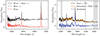 |
Fig. C.2. Left: Example of the host subtraction procedure on spectrum 3. Right: Example of the power-law and Fe II fitting and subtraction procedure on the red residuals of the left panel. The gray-shaded regions indicate where the power law is fit. |
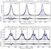 |
Fig. C.3. Emission line fitting procedure examples. Top: Example on the Hα line in spectrum 3. The three panels show, respectively, the best fit model obtained with one, two, or three Gaussians, and their respective residuals. The spectrum is represented by the black markers while the blue lines show the individual Gaussian components. The semitransparent band shows the 3σ uncertainty of the total model. The vertical dashed line indicates the rest-frame centroid of Hα. Bottom: Example on the triple-peaked Hβ line in spectrum 5. The vertical dashed line indicates the rest-frame Hβ centroid. |
All Tables
All Figures
|
Fig. 1. LS10 grz-color image of the host galaxy of J012026. The purple circle indicates the eRASS2 positional error, and the yellow circle the Swift/XRT positional error. |
| In the text | |
|
Fig. 2. Multiwavelength light curve of J012026. Top panel: X-ray evolution in the 0.2–2.3 keV band (empty triangles correspond to upper limits). Middle panel: WISE W1 and W2 light curve presented in AB magnitudes. Bottom panel: Difference-photometry light curve for the ATLAS o and c filters in μJy. The vertical dashed lines indicate the eRASS2 discovery. The numbered ticks at the top of the plot indicate the epochs at which optical spectroscopy was collected (see Sect. 5). |
| In the text | |
|
Fig. 3. eROSITA eROday 0.2–2.0 keV band light curve of J012026. The empty red circles show the source vignetting and exposure corrected count rates, while the gray triangles correspond to the background count rate. The filled red circles correspond to the eROdays selected as flaring. The time (x) axis is in units of days since the first observation of the source, for each scan. |
| In the text | |
|
Fig. 4. 0.2–2.3 keV flux vs. spectral photon index for X-ray detections. Filled red markers correspond to eROSITA flaring states and empty markers to the baseline spectra. We do not include eRASS4 due to its low flux level. |
| In the text | |
|
Fig. 5. Observed and modeled SED of J012026. The purple squares represent, respectively, the GALEX, DECam g, r, i, z, and W1 − W4 observed fluxes, while the red dots represent the model-predicted fluxes. The orange, gray, and blue lines represent the best-fit individual model components, which are respectively stellar, nebular, and dust emission. The black line is the total best-fit model. |
| In the text | |
|
Fig. 6. Normalized rest-frame follow-up spectra of J012026, offset by an arbitrary factor for visualization purposes. The most significant emission lines are indicated with dashed lines, and the gray-shaded area shows the prominent Fe II complex. Above each spectrum, we report the ID and phase since the eRASS2 discovery in days. |
| In the text | |
|
Fig. 7. Line parameter evolution of J012026. In the top-left panel, we plot the limit on the velocity resolution of the follow-up spectra with dotted lines. In the top-right panel, we plot the theoretical values of an unobscured system of the corresponding color ratios with dotted lines. |
| In the text | |
|
Fig. 8. Modeling of the triple-peaked Hβ line with a narrow Gaussian plus the E95 elliptical disk model. The green band shows the best-fit model, and the vertical dashed line corresponds to the rest-frame centroid of Hβ. |
| In the text | |
|
Fig. 9. Comparison of spectrum 3 of J012026 with examples of the different transient classes discussed transients: BFFs (In green, AT 2021loi; Makrygianni et al. 2023, AT 2019avd; Malyali et al. 2023a; Frederick et al. 2021, and AT 2022fpx; Koljonen et al. 2024), TDEs with Bowen features (in blue, ASASSN-14li; Holoien et al. 2016, AT 2022wtn; Onori et al. 2025, AT 2019dsg; van Velzen et al. 2021a, AT 2018dyb; Leloudas et al. 2019, and iPTF15af, Blagorodnova et al. 2019), and TDEs with coronal lines (in yellow, AT 2017gge, Onori et al. 2022, and AT 2022upj, Newsome et al. 2024). The gray-shaded areas show, respectively from left to right, the wavelength corresponding to Hδ, Hγ, N III, He III, Hβ and [O III]λ5007. The presented spectra are retrieved from the transient name server or from the ESO archive. |
| In the text | |
|
Fig. A.1. eRASS:5 image of J012026 and the nearby AGN WISEA J012025-292637. The image had been smoothed for visualization purposes. The white circle represents the extraction region of J012026 used in the procedure to estimate the contamination, and the cyan circle is the region used for WISEA J012025-292637. |
| In the text | |
|
Fig. A.2. eROSITA eROday 0.2-2.3 keV band light curve of J012026 (red) and WISEA J012025-292637 (blue) extracted respectively with regions of 15" and 40" in radius. The gray triangles correspond to the background count rate |
| In the text | |
|
Fig. A.3. eROSITA images of J012026. The images have been smoothed for visualization purposes, and the white circle represents a region of 60" in radius. |
| In the text | |
|
Fig. A.4. X-ray spectra of J012026. The observation name is reported in the title. All panels show, respectively with black and gray markers, the source and background counts, which have been re-binned for visualization purposes. The left panels show the DISKBB fit (dashed black line) with 1σ uncertainties (blue band), while the right panels show the same results for the power-law model (black dashed line and pink band). In all panels, the orange line shows the background model. |
| In the text | |
|
Fig. A.4. Continued. |
| In the text | |
|
Fig. A.4. Continued. |
| In the text | |
|
Fig. A.4. Continued. |
| In the text | |
|
Fig. A.4. Continued. |
| In the text | |
|
Fig. A.5. Distribution of the Pearson correlation coefficient, r. The continuous vertical line indicate the median value of r = −0.56, and the dashed line shows r = 0. The gray-shaded area indicates the 95% confidence interval. |
| In the text | |
|
Fig. C.1. Archival 2dF spectrum of the nucleus of J012026. The black vertical lines show the rest-frame wavelengths of the Ca H & K doublet, Hβ, and the [O III] doublet. The spikes slightly redward of the [O III] doublet and around ∼ 5700 Å are likely artifacts. |
| In the text | |
|
Fig. C.2. Left: Example of the host subtraction procedure on spectrum 3. Right: Example of the power-law and Fe II fitting and subtraction procedure on the red residuals of the left panel. The gray-shaded regions indicate where the power law is fit. |
| In the text | |
|
Fig. C.3. Emission line fitting procedure examples. Top: Example on the Hα line in spectrum 3. The three panels show, respectively, the best fit model obtained with one, two, or three Gaussians, and their respective residuals. The spectrum is represented by the black markers while the blue lines show the individual Gaussian components. The semitransparent band shows the 3σ uncertainty of the total model. The vertical dashed line indicates the rest-frame centroid of Hα. Bottom: Example on the triple-peaked Hβ line in spectrum 5. The vertical dashed line indicates the rest-frame Hβ centroid. |
| In the text | |
Current usage metrics show cumulative count of Article Views (full-text article views including HTML views, PDF and ePub downloads, according to the available data) and Abstracts Views on Vision4Press platform.
Data correspond to usage on the plateform after 2015. The current usage metrics is available 48-96 hours after online publication and is updated daily on week days.
Initial download of the metrics may take a while.