| Issue |
A&A
Volume 701, September 2025
|
|
|---|---|---|
| Article Number | A260 | |
| Number of page(s) | 42 | |
| Section | Extragalactic astronomy | |
| DOI | https://doi.org/10.1051/0004-6361/202555362 | |
| Published online | 24 September 2025 | |
The ALMA-CRISTAL survey: Resolved kinematic studies of main sequence star-forming galaxies at 4 < z < 6
1
Max-Planck-Institut für Extraterrestrische Physik (MPE), Gießenbachstra. 1, D-85748 Garching, Germany
2
Departamento de Astronomía, Universidad de Concepción, Barrio Universitario, Concepción, Chile
3
Millenium Nucleus for Galaxies (MINGAL), Concepción, Chile
4
Purple Mountain Observatory, Chinese Academy of Sciences, 10 Yuanhua Road, Nanjing 210023, China
5
Space Telescope Science Institute, 3700, San Martin D, MD 21218, USA
6
Department of Physics and Astronomy and PITT PACC, University of Pittsburgh, Pittsburgh, PA 15260, USA
7
Departments of Physics and Astronomy, University of California, Berkeley, CA 94720, USA
8
Max-Planck-Institut für Astrophysik (MPA), Karl-Schwarzschild-Str. 1, D-85748 Garching, Germany
9
Instituto de Estudios Astrofísicos, Facultad de Ingeniería y Ciencias, Universidad Diego Portales, Av. Ejército Libertador 441, [Código Postal 8370191] Santiago, Chile
10
Department of Astronomy, University of Virginia, 530 McCormick Road, Charlottesville, VA 22903, USA
11
National Radio Astronomy Observatory, 520 Edgemont Road, Charlottesville, VA 22903, USA
12
Jodrell Bank Centre for Astrophysics, Department of Physics and Astronomy, School of Natural Sciences, The University of Manchester, Manchester M13 9PL, UK
13
Universitäts-Sternwarte Ludwig-Maximilians-Universität (USM), Scheinerstr. 1, München D-81679, Germany
14
Centre for Astrophysics and Supercomputing, Swinburne University of Technology, Hawthorn 3122, Australia
15
Sterrenkundig Observatorium, Ghent University, Krijgslaan 281 S9, B-9000 Ghent, Belgium
16
Institute of Astrophysics, Foundation for Research and Technology – Hellas (FORTH), Heraklion 70013, Greece
17
School of Sciences, European University Cyprus, Diogenes Street, Engomi, 1516 Nicosia, Cyprus
18
Las Campanas Observatory, Carnegie Institution of Washington, Casilla 601, La Serena, Chile
19
Department of Astronomy, School of Science, SOKENDAI (The Graduate University for Advanced Studies), 2-21-1 Osawa, Mitaka, Tokyo 181-8588, Japan
20
National Astronomical Observatory of Japan, 2-21-1 Osawa, Mitaka, Tokyo 181-8588, Japan
21
Department for Astrophysical & Planetary Science, University of Colorado, Boulder, CO 80309, USA
22
Department of Physics and Astronomy and George P. and Cynthia Woods Mitchell Institute for Fundamental Physics and Astronomy, Texas A&M University, 4242 TAMU, College Station, TX, 77843-4242, USA
23
Dept. Fisica Teorica y del Cosmos, E-18071 Granada, Spain
24
Instituto Universitario Carlos I de Fisica Teorica y Computacional, Universidad de Granada, E-18071 Granada, Spain
25
Osservatorio Astronomico di Padova, Vicolo dell’Osservatorio 5, Padova I-35122, Italy
26
School of Physics and Astronomy, Tel Aviv University, Tel Aviv 69978, Israel
27
Centre for Computational Astrophysics, Flatiron Institute, 162 5th Avenue, New York, NY 10010, USA
28
Faculty of Engineering, Hokkai-Gakuen University, Toyohira-ku, Sapporo 062-8605, Japan
29
Department of Astronomy and Joint Space-Science Institute, University of Maryland, College Park, MD 20742, USA
⋆ Corresponding author: This email address is being protected from spambots. You need JavaScript enabled to view it.
; This email address is being protected from spambots. You need JavaScript enabled to view it.
Received:
2
May
2025
Accepted:
15
July
2025
Abstract
We present a detailed kinematic study of a sample of 32 massive (9.5 ⩽ log(M*/M⊙) ⩽ 10.9) main sequence star-forming galaxies (MS SFGs) at 4 < z < 6 from the ALMA-CRISTAL programme. The data consist of deep (up to 15 hr observing time per target), high-resolution (∼1 kpc) ALMA observations of [C II]158 μm line emission. This dataset allowed us to carry out the first systematic, kiloparsec-scale (kpc-scale) characterisation of the kinematics nature of typical massive SFGs at these epochs. We find that ∼50% of the sample are disk-like, with a number of galaxies located in systems of multiple components. Kinematic modelling reveals these main sequence disks exhibit high-velocity dispersions (σ0), with a median disk velocity dispersion of ∼70 km s−1 and Vrot/σ0 ∼ 2, which is consistent with dominant gravity driving. The elevated disk dispersions are in line with the predicted evolution based on Toomre theory and the extrapolated trends from z ∼ 0–2.5 MS star-forming disks. The inferred dark matter (DM) mass fraction within the effective radius fDM(< Re) for the disk systems decreases with the central baryonic mass surface density. This is consistent with the trend reported by kinematic studies at z ≲ 3; roughly half the disks display fDM(< Re)≲ 30%. The CRISTAL sample of massive MS SFGs provides a reference of the kinematics of a representative population and extends the view onto typical galaxies beyond previous kpc-scale studies at z ≲ 3.
Key words: galaxies: evolution / galaxies: high-redshift / galaxies: kinematics and dynamics / submillimeter: galaxies
© The Authors 2025
 Open Access article, published by EDP Sciences, under the terms of the Creative Commons Attribution License (https://creativecommons.org/licenses/by/4.0), which permits unrestricted use, distribution, and reproduction in any medium, provided the original work is properly cited.
This article is published in open access under the Subscribe to Open model.
Open access funding provided by Max Planck Society.
1. Introduction
Studying the kinematics of high-redshift galaxies offers a direct tracer of the distribution of stars, gas, and dark matter (DM) on galactic scales. Observations at multiple epochs provide constraints on the evolution of the contribution of rotation and turbulence to the dynamical support of galaxies. Therefore, galaxy kinematics serve as a powerful probe of the dominant mechanisms governing the growth and structural formation of galaxies, with processes including gas accretion, non-circular motions, galaxy interactions, and feedback.
Thanks to the advent of near-infrared (NIR) integral field units (IFU) and slit spectroscopy on 8–10 m telescopes (e.g. Eisenhauer et al. 2003; Sharples et al. 2013), ionised gas kinematics from rest-frame optical emission lines have become routinely accessible at cosmic noon z ∼ 1–3. This has enabled the census of resolved kinematics of massive star-forming galaxies (SFGs) at z ∼ 1–3 on the main sequence (MS) of star-forming galaxies (SFGs, e.g. Förster Schreiber et al. 2009; Kassin et al. 2012; Wisnioski et al. 2015), which dominate the population and cosmic star formation rate density (Madau & Dickinson 2014). The cold gas kinematics of the same population of galaxies traced primarily via CO lines are increasingly available through the Atacama Large Millimeter/submillimeter Array (ALMA) and Northern Extended Millimetre Array (NOEMA) and employed in a number of recent studies (Übler et al. 2018; Nestor Shachar et al. 2023; Rizzo et al. 2023; Liu et al. 2023).
The general findings at z ≲ 3 suggest that a majority of disks among massive (stellar masses M⋆ ≳ 1010 M⊙) SFGs have increasing gas velocity dispersion, σ0, and decreasing rotational-to-dispersion support, Vrot/σ0, towards higher redshift. These findings are in line with the increase of galactic gas mass fractions, which play an important role in the emergence of the ‘equilibrium growth’ model of galaxy evolution (see reviews by Tacconi et al. 2020, and references therein) in the framework of marginally stable gas-rich disks (e.g. Genzel et al. 2008; Dekel et al. 2009; Dekel & Burkert 2014; Zolotov et al. 2015; Ginzburg et al. 2022). These works have highlighted the important role of internal processes, alongside accretion and merging, in galaxy stellar mass and structural build-up during the peak epoch of cosmic star formation activity around z ∼ 2 (see e.g. reviews by Glazebrook 2013; Förster Schreiber & Wuyts 2020).
The exploration of kinematics beyond cosmic noon at z > 3 has been opened by facilities such as ALMA and NOEMA, primarily via the bright [C II]2P3/2–2P1/2 ([C II]158 μm, hereafter [C II]) line emission. The [C II] line serves as a key coolant for the interstellar medium (ISM; e.g. Wolfire et al. 2003). Its relatively low ionisation potential of 11.3 eV (compared to 13.6 eV for hydrogen) allows [C II] to arise from various ISM phases, primarily from the photo-dissociation regions (PDRs; e.g. Vallini et al. 2015; Clark et al. 2019). Consequently, the [C II] line is an ideal tracer for kinematics, enabling measurements reaching well beyond the effective radii of these early galaxies (e.g. Lelli et al. 2021; Jones et al. 2021; Tsukui & Iguchi 2021; Umehata et al. 2025).
So far, studies suggest that disks appear to be sub-dominant among the bulk of SFGs at z ∼ 4−7 (from rest-UV-selected samples, e.g. Smit et al. 2018; Le Fèvre et al. 2020; Jones et al. 2021; Herrera-Camus et al. 2022; Posses et al. 2023). While some of them appear to be quite turbulent, high-resolution observations of small samples of individual galaxies, primarily IR-luminous dusty SFGs, reveal the existence of dynamically cold disks at those early epochs (e.g. Sharda et al. 2019; Fraternali et al. 2021; Lelli et al. 2021; Rizzo et al. 2021; Tsukui & Iguchi 2021; Roman-Oliveira et al. 2023; Rowland et al. 2024). Larger, more systematic samples covering typical galaxies, such as those provided by ALPINE (4 < z < 6; Le Fèvre et al. 2020; Béthermin et al. 2020; Faisst et al. 2020a) and REBELS (7 < z < 8; Bouwens et al. 2022), are available, albeit at lower spatial resolution and shallower depths. Nevertheless, the typical SFGs targeted by ALPINE formed an ideal sample for high-resolution follow-up studies, providing the motivation for the CRISTAL ([C II] Resolved ISM in STar forming galaxies with ALMA) survey.
CRISTAL is designed to address four primary science goals: (i) kinematics, (ii) outflows, (iii) spatial distribution of the ISM and star formation, and (iv) the ISM conditions.
Herrera-Camus et al. (2022) presented a pilot study of the kinematics of one of the CRISTAL galaxies, HZ4 (CRISTAL-20). Posses et al. (2025) and Telikova et al. (2025) presented detailed case studies of the kinematics of CRISTAL-05 and CRISTAL-22, respectively, and highlighted the improvement in kinematics modelling of complex systems, thanks to higher resolution. The outflow properties of one of the CRISTAL galaxies are presented in Davies et al. (2025) and the overall outflow demographics through stacking in Birkin et al. (2025). Works addressing goals (iii) and (iv) are presented in Li et al. (2024), Mitsuhashi et al. (2024), Villanueva et al. (2024), Ikeda et al. (2025), Lines et al. (2025), and Solimano et al. (2025). We refer to the overview survey paper by Herrera-Camus et al. (2025) for more details. In this paper, we present a systematic study of the kinematics of the CRISTAL sample.
The structure of this paper is as follows. In Sect. 2, we describe the sample selection and data reduction process. Sect. 3 presents the classification of the kinematic types and Sect. 4 discusses the disk fraction of CRISTAL galaxies. Sect. 5 discusses the kinematic properties of the disks from forward modelling, along with a comparison with literature results in the context of the dynamical evolution of MS SFGs. Sect. 6 investigates the intrinsic velocity dispersion of CRISTAL disks in the broader context of the dynamical evolution of galaxies with redshift, exploring possible drivers of turbulence, in particular, gravitational instabilities and stellar feedback. In Sect. 7, we discuss the DM fraction within the effective radius of the CRISTAL disks, and its dependence on the circular velocity and baryonic surface density. Sect. 8 presents a brief discussion on the properties of non-disk galaxies. Finally, Sect. 9 summarises the key findings and outlines ways forward to improve constraints on the nature and kinematics of z ∼ 4–6 galaxies.
Throughout, we adopted a flat ΛCDM cosmology with H0 = 70 km s−1 Mpc−1, and Ωm = 0.3. Physical size is always reported in physical kiloparsecs (pkpc), but we use kpc henceforth for brevity. Where relevant, we quote the rest-frame air wavelengths unless specified otherwise.
2. Data and sample selection
2.1. Galaxy sample
The full CRISTAL sample is presented by Herrera-Camus et al. (2025). In brief, the survey builds on an ALMA Cycle-8 Large Program (2021.1.00280.L; PI: R. Herrera-Camus), targeting [C II] emission of 19 MS SFGs drawn from ALPINE (Le Fèvre et al. 2020), selected at log(M⋆/M⊙) ⩾ 9.5 and within a factor of 3 of the MS in their specific SFRs (sSFR/sSFR(MS) ⩽ 3). At the higher resolution of the CRISTAL ALMA observations, some of these sources split into separate components. This sample was expanded with six systems satisfying the same criteria taken from pilot programmes and the literature (see details in Herrera-Camus et al. 2025). There are 39 galaxies in the final CRISTAL sample in total.
The sample studied here consists of the 32 galaxies near the MS that have sufficient S/N and are sufficiently well-resolved to perform quantitative measurements and model their kinematic properties. Table 1 lists the galaxies included in this kinematics sample, along with their redshifts, coordinates, stellar masses (M⋆) and SFRs, as well as the beam size and sensitivity of the ALMA data sets. Fig. 1 shows the range of M⋆, SFRs, and surface densities in SFR and baryonic masses (ΣSFR and Σbar) covered by the CRISTAL MS SFGs, in comparison to those drawn from selected detailed kinematics studies of disks at lower redshifts in ionised and cold molecular gas, and literature work at z ≳ 4 from [C II] data (Neeleman et al. 2020; Rizzo et al. 2020, 2021; Fraternali et al. 2021; Herrera-Camus et al. 2022; Parlanti et al. 2023; Roman-Oliveira et al. 2023). CRISTAL MS SFGs are distinct from most existing samples that predominantly comprise starburst or compact galaxies, allowing for more direct comparisons to z ∼ 1–3 kinematics studies of MS star-forming disks at lower redshifts (e.g. Wisnioski et al. 2015, 2019; Genzel et al. 2020; Nestor Shachar et al. 2023; Puglisi et al. 2023). For the purpose of the figures, we adopted the values from the ALPINE catalogues (Béthermin et al. 2020; Faisst et al. 2020a; Le Fèvre et al. 2020) to demonstrate the original sample selection. We adopted the values given in Table 1 for our subsequent analysis in this work.
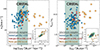 |
Fig. 1. Parameter space of the CRISTAL sample in terms of surface densities of star formation rate (ΣSFR, left) and baryons (Σbar, right). For comparison, the z ∼ 2 MS galaxies observed in Hα (blue circles) and CO (red hexagons) by Nestor Shachar et al. (2023) are also shown. The inset of the left and right panels show the SFR-M⋆ and [C II]-sizes-M⋆ distributions of CRISTAL (green contour) and other studies at z ≳ 4 (yellow diamonds) (Neeleman et al. 2020; Rizzo et al. 2020, 2021; Fraternali et al. 2021; Herrera-Camus et al. 2022; Parlanti et al. 2023; Roman-Oliveira et al. 2023), respectively. The solid line in the left inset is the MS relation from Speagle et al. (2014) at z = 5, with the shading representing ±0.5 dex offset from the relation. For the purposes of illustration, the values of CRISTAL shown on the plots are adopted from ALPINE (Béthermin et al. 2020; Faisst et al. 2020a; Le Fèvre et al. 2020). CRISTAL provides a higher-resolution sample of MS SFGs that fills up the parameter space currently poorly explored by existing z ≳ 4 samples observed with [C II], which predominantly comprises starburst and compact galaxies. |
Properties of the 32 galaxies in kinematics sample of ALMA-CRISTAL.
2.2. ALMA observations and data
We refer to Herrera-Camus et al. (2025) for the observation setup. In brief, each observation was reduced using the standard CASA (Common Astronomy Software Applications; CASA Team et al. 2022) pipeline. Each cube was continuum-subtracted in the uv plane, resulting in a line-only, continuum-free data cube. For the kinematics modelling, we used the cubes with channel with of 20 km s−1 and natural weighting1. We did not apply the ‘JvM’ correction (Jorsater & van Moorsel 1995) in our analysis, as it mostly affects the measurement of integrated properties.
2.3. Space-based ancillary data
All of the galaxies in the kinematics sample benefit from high-resolution broad-band optical to mid-IR imaging obtained with the Hubble Space Telescope (HST) and, in most cases, also the James Webb Space Telescope (JWST). Covering stellar continuum emission at rest-frame UV to near-IR wavelengths, this imaging data provides important complementary information for a full morpho-kinematic classification and important priors in the dynamical modelling of [C II] kinematics. These data sets were reduced in a homogeneous fashion for the CRISTAL sample, as described by Li et al. (2024) and Herrera-Camus et al. (2025).
3. (Morpho)-kinematic classification
In this section, we describe the classification of the galaxies from the CRISTAL kinematics sample. We used several methods devised for applications to IFU and interferometric observations of high-redshift galaxies, with a comparable S/N and resolution as our ALMA data. We determined the final classification by combining the results from each method detailed in Sects. 3.1–3.5. We assigned two points to three metrics (PV, kinemetry, and spectro-astrometry) and one point to Vobs/2σ and morphological information, amounting to eight points.
Table 2 compiles the relevant measurements and resulting classification. Appendix A provides details of the individual galaxies. In summary, the systems in the CRISTAL sample can be broadly classified into three general groups:
-
Best Disk (22%): Score ⩾ 7. These are clear disks with no clear sign of nearby interacting companions within a projected distance of ∼20 kpc in the HST, JWST, and ALMA data. The velocity gradients are monotonic with a well-defined kinematic position angle (PAk), and the location of steepest slope coinciding with a central peak in observed velocity dispersion, defining the kinematic centre.
-
Disk (28%): Score = 5–6. They show features of a rotating disk, but also irregularities. These systems meet most criteria but exhibit some deviations from one or the other pure disk rotation features. Except for two cases, they belong to systems with visible companions in both [C II] and HST or JWST imaging data.
-
Non-Disk (50%): The rest of the systems with a score of ⩽4. They do not have an apparent velocity gradient across ⩾2 beams and no centralised dispersion peak. Some of them have a visible companion.
3.1. Position-velocity diagrams
We extracted position-velocity (p-v) diagrams from the original reduced data cubes along the kinematic major axis (PAk), defined as the direction of the largest observed velocity difference across the source. The width of the synthetic slit is equal to the FWHM of each beam, which was taken to be the geometric average of the major and minor axes values listed in Table 1. The slit was positioned to pass through the dynamical centre of the galaxies. We then integrated the light along the spatial direction perpendicular to the slit orientation. These p-v diagrams are presented in Figs. A.5 to A.7 in Appendix A. For visualisation purposes, we median-filtered the p-v diagrams with a kernel size of 3 pixels.
We classified a system as disk-like if there are no detached and distinct velocity structures in the p-v diagrams. This metric contributes to two points in the disk score in Table 2. We did not consider deviations (e.g. CRISTAL-02 and 08) from a standard S-shape as indicative of a merger, as they may instead reflect the possible origin of non-circular gas flow, which could be common for gas-rich systems at higher redshifts.
3.2. Kinematics profiles and Vobs/2σint
The ratio between the full observed velocity difference across a source (Vobs) and the source-integrated line width (σint) has been used as a proxy to distinguish systems with dominant support from rotational and orbital motions versus random motions (e.g. Förster Schreiber et al. 2009; Wisnioski et al. 2015). The Vobs and σint values can be measured from the data, without the need for beam-smearing or inclination corrections. The boundary at Vobs/2σint = 0.4 adopted in previous work, based on mock disk models, is also applicable for the typical range of galaxy sizes relative to beam sizes for our sample.
We measured the integrated line width, σint, from spatially integrated spectra extracted from the reduced data cubes. The cubes are at the original spatial and spectral resolution and with the channel size of ΔV = 20 km s−1. The circular apertures for the extraction are positioned at the light centre of the galaxies, determined from the [C II] line maps, in order to capture the contributions from both velocity gradients and local velocity dispersion to σint. The apertures’ sizes roughly followed those determined by Ikeda et al. (2025). We then summed the spectra of individual pixels within the apertures to obtain the integrated spectrum. The extracted spectra are shown in the last column of Figs. A.5 to A.7 in Appendix A.
We fitted the spectrum with a single Gaussian with emcee (Foreman-Mackey et al. 2013) to extract the line widths, except for CRISTAL-02, where we fit a double Gaussian profile as there is a broad component possibly associated with an outflow (Davies et al. 2025). The emission from the narrow component is always the one used in this analysis.
The fitted values of integrated line widths (σint([C II])) are annotated in Figs. A.5 to A.7 along with the best-fit model overlaid on the extracted spectra. Uncertainties of σint([C II]) are taken as the [16, 84]-th percentile (1σ) bounds of the marginalised posterior distributions. We stress that the σint quantity determined here does not represent the local intrinsic disk velocity dispersion, but rather a global measure of the dynamical support combining rotation and orbital motions as well as random motions.
The value of Vobs is defined as the maximum observed velocity difference Vobs = Vmax − Vmin. We extract velocity profiles from the p-v diagrams obtained in Sect. 3.1 by fitting a single Gaussian profile column-by-column (i.e., collapsed emission of the velocity channels at the same position) using again emcee (Foreman-Mackey et al. 2013). A one-pixel-wide vertical pseudo-slit is moved along the position axis. The centroids and widths of the fitted Gaussian models would then be the velocity and velocity dispersion at the locations of the slits. Finally, the extracted profiles were down-sampled by averaging to a resolution of one-half to one-fourth of the beam FWHM. The velocity and velocity dispersion profiles can then serve as an input for the dynamical modelling in Sect. 5.
We list the Vobs/2σint of our sample in Table 2. We plot in Fig. 2 the distribution of Vobs/2σint as a function of the stellar mass. For comparison, we show the values for the SINS Hα IFU sample at z ∼ 2 (Förster Schreiber et al. 2009). The median Vobs/2σint of all samples is 0.56. For the Best Disk, Disk and Non-Disk samples, the median values are 0.73, 0.45, and 0.57, respectively.
Kinematic classification and properties of CRISTAL galaxies.
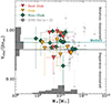 |
Fig. 2. Ratios of observed half velocity gradient Vobs/2 and integrated line width (σint) of [C II] as a function of stellar mass M*. The black horizontal dashed line represents the distinction value (Vobs/2σint = 0.4), which demarcates the boundary between rotation- and dispersion-dominated systems, as commonly used in the literature. |
We observe that many Non-Disk systems have Vobs/2σint > 0.4, which can be attributed to the fact that mergers may exhibit a substantial projected velocity gradient from orbital motions, depending on the orientation of the merging system. While the Vobs/2σint ratio is useful, especially in cases where the sources are less well resolved, it is not sufficient to unambiguously distinguish disks from mergers. Therefore, this metric contributes only one point to the disk score, as reported in Table 2.
3.3. Velocity and velocity dispersion maps and their asymmetry
To derive the flux, velocity, and velocity dispersion maps, we fitted a single Gaussian profile to the [C II] emission line of each spaxel in the continuum-subtracted line cube in velocity units, with the amplitude, mean and standard deviation of the profile as free parameters. In the resulting [C II] kinematic maps, we masked pixels with S/N < 3 and pixels resulting in unphysical outlier values. For the velocity map, we determined the systemic velocity of the galaxy by symmetrising the red-shifted and blue-shifted peak velocities. Fig. 3 displays the derived velocity and velocity dispersion maps, plotted in the M⋆ versus offset from the MS in SFR. The line flux, velocity, and velocity dispersion maps of individual galaxies are shown in the fourth and fifth columns of Figs. A.5–A.7 in Appendix A.
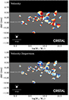 |
Fig. 3. Velocity (top) and velocity dispersion (bottom) fields of CRISTAL galaxies placed on the ΔMS offset relative to the Speagle et al. (2014) MS relation. The velocity and dispersion fields correspond to those derived from the [C II] emission described in Sect. 3.3. For the velocity fields, the colour coding represents the relative velocity of the line emission with respect to the systemic velocity. For the dispersion fields, the colour coding indicates the widths (in standard deviation) of the 1D Gaussian fitted to the spectra of individual spaxels. All sources are shown in the same field of view of 3″ (∼20 kpc at z ∼ 5). The median beam size (0 |


Under the assumption of a single Gaussian profile, our fits primarily capture the narrower line emission component dominated by star formation. Such single-component fits of individual pixel spectra will scarcely be sensitive to possible emission from broader lines originating, e.g. from outflowing gas as long as the amplitude of the broad component is sufficiently low (e.g. Förster Schreiber et al. 2018). Examination of our CRISTAL data shows this is the case for all galaxies considered here except for CRISTAL-02, where more prominent outflow components are detected (Davies et al. 2025). In the kinematic maps of these galaxies, the regions (largely outside of the main body of the sources) are masked out for quantitative analysis.
We then use kinemetry (Krajnović et al. 2006) to quantify asymmetries in the velocity and velocity dispersion maps of our galaxies. We followed the method described by Shapiro et al. (2008) for applications in studies of galaxy kinematics at z ∼ 2 (see also, e.g. Swinbank et al. 2012; Genzel et al. 2023).
Kinemetry allows us to perform a Fourier analysis on the velocity and dispersion maps, decomposed into concentric ellipses, with the centre, position angle (PA), and inclination determined a priori through methods detailed in Sect. 3.1. Given the limited S/N and angular resolution of our data, we fixed the centre, PAk, and inclination to the adopted values in Sects. 3.1 and 5, respectively. We also required at least 75% of valid pixels in an annulus. We followed the Fourier expansion up to the fifth-order term, similar to Shapiro et al. (2008).
We used the demarcation set by Shapiro et al. (2008) at Kasym =  = 0.5, above which the system is classified as a merger and below which is a disk. The values of vasym and σasym are dimensionless measurements of the average higher-order kinematic coefficients in the Fourier expansion relative to the coefficients corresponding to the regular rotation.
We plot the vasym and σasym of the CRISTAL galaxies in Fig. 4. There are 20 and 10 galaxies (out of 30 with measurements) that fall into the ‘disk’ and ‘merger’ regime, respectively, according to the fiducial Kasym = 0.5. Some Disks and Non-disks (according to the overall classification) overlap in the region around the boundary, which can reflect intrinsic deviations from pure circular motions caused by minor merging, non-axisymmetric structures such as bars and spirals, even in the absence of interactions, noise in kinematic maps or incomplete coverage of the objects due to regions with lower S/N and fainter surface brightness, beam smearing, or a combination of these factors. For illustrative purposes, we indicate in Fig. 4 the band corresponding to Kasym = 0.3 to 0.9, for the simulated galaxies used by Shapiro et al. (2008), to calibrate the threshold would result in 6% higher merger fraction or 3% higher disk fraction, respectively. Adopting the fiducial threshold for CRISTAL, we classified galaxies with Kasym ⩽ 0.5 as a disk, counting for two points in the disk score from this metric.
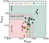 |
Fig. 4. Asymmetry measure of the velocity and velocity dispersion fields for the CRISTAL galaxies from Kinemetry (Krajnović et al. 2006) is shown in Fig. 4. The black dashed line represents the demarcation in Shapiro et al. (2008) at Kasym = 0.5. With this metric alone, we classify a system as disk-like if it falls below the dashed line and as a merger if it falls above. Over half of the samples fall below the dashed line. The pink (Kasym = 0.9) and green (Kasym = 0.3) lines indicate the modified demarcations. |
3.4. Spectro-astrometry
We also applied spectro-astrometry (SA) to classify our sample. This technique, commonly used to study compact, marginally resolved stellar binary systems (e.g. Christy et al. 1981; Beckers 1982) was successfully applied to IFU observations of high-z galaxies (e.g. Gnerucci et al. 2010; Perna et al. 2025). SA operates on the principle that closely spaced sources with projected separation below the angular resolution element can be spectrally separated if their relative velocities differ. This technique leverages the 3D information in data cubes and can be especially useful in retrieving velocity gradients when beam smearing is important.
For each velocity channel map, we derived the spatial offsets along the X and Y directions by fitting a 2D Gaussian without any a priori assumptions of the kinematics major axis. In cases where multiple emission peaks were observed and separated by multiple beams in FWHM, we fitted multiple 2D Gaussians to the emission blob. We derived the positional uncertainty following Eq. (1) in Condon et al. (1998), which depends on the amplitude of the emission and the beam size, in addition to the formal fitting errors. We show the locus traced by the SA measurements in the sixth column in Figs. A.2–A.4 in Appendix A, overlaid on either HST or JWST colour images.
For a galaxy to be considered Best Disk, its SA locus should be unidirectional, i.e., moving along monotonically in one direction, as in the case of CRISTAL-15 and 20 (Fig. A.2). However, for systems with non-circular motion, the loci would deviate from a straight line near the centre, as in the case of CRISTAL-02 and 08, but would overall follow a single direction. In all cases, the overall direction of the velocity gradients agrees with the velocity map with consistent PAkin. For Non-disks, the SA loci would exhibit a more zig-zag shape, characterised by sudden changes in opposite direction; when companions are present, the loci show discontinuities with abrupt jumps from one location to another, often separated by one to two resolution elements.
The inherent nature of SA results in uneven spatial sampling, while spectral sampling remains constant. The spectral resolution of our SA measurement is naturally determined by the channel width, which is set at 20 km s−1. We did not consider a wider channel width, such as e.g. 50 km s−1 because it would have poorly compromised spectral sampling for several sources with observed velocities vobs < 200 km s−1 (Table 2). In the case of Non-Disk sources, which could potentially be mergers, there could be a few channels with emission peaks that are spatially close to each other. Although this may appear to be a spatial sampling that is too high on the SA curve, we have chosen to retain these data, as they could indicate unresolved line-of-sight mergers.
The fainter outer regions of the sources, often associated with the most blue- or redshifted emission, tend to have too low S/N for a robust centroid measurement. Consequently, the full velocity gradient may not be probed for some of our targets.
This metric adds two points to the disk score in Table 2.
3.5. Morphology of rest-frame UV-optical and [C II] line emission
We complement the kinematic classification methods described in the previous sections with morphological information. We consider the HST along with JWST/NIRCam data and [C II] data. The longest wavelength NIRCam filter F444W corresponds to the rest-frame optical emission (λ = 0.7 μm) at z = 5, redwards of the Balmer break, in contrast to the rest-frame 0.3 μm provided by HST/F160W. The depth of the JWST data varies across the sample, with CRISTAL-08, 11, 13, and 15 being the deepest.
We considered the source multiplicity in our inspection of the imaging data. In most cases, our ALMA data already indicate the single or multiple nature of the galaxies, with 14 of the multiple systems associated with Non-Disks according to the kinematic criteria applied in Sects. 3.1–3.4. The higher angular resolution of JWST can provide a more detailed view of the morphology and deblending unresolved companions within the ALMA beam that could explain the observed perturbations in the [C II] kinematics. We emphasise that the companions we defined in Table 1 are unlikely to be multiple clumps within a single galaxy, as their closest separations is on average ∼8 kpc, ranging from 5 to 10 kpc, which is much larger than the typical size of SFGs at z ∼ 5 (Varadaraj et al. 2024; Miller et al. 2025). We further stress that multiplicity on scales of a few kpc could be ambiguous, as clumpy disks may mimic multiple systems, especially if the sensitivity is insufficient to detect a fainter host galaxy underlying bright clumps.
The first two columns of Figs. A.2–A.4 present a comparison between HST and JWST colour-composite images. We observe a marked difference between the rest-frame optical and UV images of galaxies in CRISTAL-01a, 07c, 08, 11, 12, 13, 16, 24, and 25. For systems CRISTAL-02 and 04a, the rest-frame optical resembles that in the UV. However, all galaxies retain their substructures or clumpy appearance. The single-pair classification using the [C II] and HST-based morphologies of Ikeda et al. (2025) are unchanged with the additional information from JWST data, and the multiplicity remains the same.
To highlight the clumpiness and substructures, we subtracted the F444W image by a smooth Sérsic (Sérsic 1968) model in Appendix B. The clumpy appearance of CRISTAL-02, 08, and 15 is apparent in the residual images shown in Fig. B.1.
Since many of the galaxies were not well-fitted by a Sérsic model, we did not consider the difference between JWST (or HST) morphological PA and PAkin (defined in Sect. 3.1) as a disk criterion because the former was not well-constrained.
There are systems with visible [C II] companions or extended emission, such as CRISTAL-01b, 12, and 13, but no associated counterparts in either HST or JWST images. This suggests that we are still missing the more evolved stellar population due to extinction or simply fainter emission with the shallow NIRCam data. Therefore, we consider the imaging data as complementary but not decisive evidence for the kinematic nature. With the visual inspection of JWST and HST images, alongside [C II] line maps, we classify a system as a disk if it is a single-component system with smooth underlying emission, possibly featuring bright clumpy substructures that are closely spaced (typically within ≲2 kpc, generally consisting of more than two clumps). Additionally, there should be no detectable companion within ≲20 kpc across the observed wavelengths. This contributes one point towards the disk score.
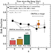 |
Fig. 5. Comparison of the CRISTAL total disk fraction (yellow hexagon with red outline) to the mass-selected sample from Ferreira et al. (2023) based on CRISTAL mass range. The grey curve with square markers shows the ‘redshift-corrected’ trend of their high-mass bin. To more fairly compare with our sample, we further selected so that their star formation rates are within 1 dex from the Speagle et al. (2014) MS relation. The grey horizontal line indicates the redshift range of CRISTAL (4.4 < z < 5.7). The black solid curve with square markers represents the redshift evolution of disk fraction as reported by Ferreira et al. (2023) before their application of ‘redshift corrections’, which primarily account for surface-brightness effects in higher redshift objects. It would be a more equal comparison since we do not apply any such correction to the CRISTAL disk fraction. The inset shows the distribution of Best Disk, Disk, and Non-disk among the CRISTAL sample. |
4. Disk fraction
Considering systems with a disk score of ⩾5, the total disk fraction among the 32 CRISTAL kinematics samples is 50 ± 9% (N = 16), encompassing both Best Disk and Disk (Table 2). The Best Disk and Disk categories make up 22 ± 7% (N = 7) and 28 ± 8% (N = 9) of the sample, respectively. The errors are binomial errors. The distribution of these types is shown in the inset in Fig. 5. The disk fraction in our study is higher than that reported in the previous ALPINE work (Le Fèvre et al. 2020), which found that for the overlapping CRISTAL sample, ≲40% of systems are classified as ‘rotator’ or ‘extended dispersion dominated’, with only < 20% being the former, and the remaining systems being classed as ‘pair-mergers’.
The 50% disk fraction of CRISTAL (4.4 < z < 5.7) is consistent with morphological studies based on NIRCam/JWST data, which reveal a high fraction of disks of ∼35% on average across studies (Ferreira et al. 2023; Jacobs et al. 2023; Kartaltepe et al. 2023; Huertas-Company et al. 2024; Lee et al. 2024; Pandya et al. 2024; Tohill et al. 2024). A smaller sample using JWST/MIRI also supports this finding (Costantin et al. 2025). These results suggest an early establishment of the Hubble sequence (Ferreira et al. 2023; Xu & Yu 2024; Huertas-Company et al. 2025).
In particular, we compare our CRISTAL disk fraction with Ferreira et al. (2023), a morphological study of ∼4000 galaxies from the CEERS survey, classified in rest-frame optical observed with JWST. Fig. 5 plots our disk fractions against their evolutionary trend. For consistency, we select galaxies from Ferreira et al. (2023) in the same mass and ΔMS ranges as our kinematic sample, using the galaxy parameters from the CANDELS-EGS catalogue of Stefanon et al. (2017). We did not apply surface-brightness corrections to the fractions as we compared them with the direct fraction from our kinematic classification. Figure 5 shows these derived morphology-based disk fractions over z ∼ 1–6; our kinematics-based disk fraction for the CRISTAL MS SFGs is in very good agreement.
The presence of Disk (disks in an interacting system) is perhaps not surprising, as hinted from simulation (see also the classic example of M51); gravitational interactions between galaxies and the presence of rotating disks are not inherently contradictory (Springel & Hernquist 2005; Robertson et al. 2006). The rotation of a disk is relatively resilient to minor mergers. For gas-rich systems, the stellar disk can rapidly reform and sustain itself through the formation of new stars from the remaining gas, even if the pre-existing stellar disk is destroyed in the process (Übler et al. 2014; Peschken et al. 2020; Sotillo-Ramos et al. 2022).
5. Kinematics modelling and properties of the disk sample
5.1. Forward modelling with DysmalPy
To extract the intrinsic kinematics and mass distribution of CRISTAL disks, we used the public forward-modelling code DysmalPy2 (Davies et al. 2004a,b; Cresci et al. 2009; Davies et al. 2011; Wuyts et al. 2016; Lang et al. 2017; Price et al. 2021; Lee et al. 2025). Table 3 reports the best-fit results. We refer to the earlier cited works for a detailed description of DysmalPy. In short, it is a forward modelling tool that starts from a parametrised input mass distribution to establish the best-fit models for the data. The models consist of a baryonic disk, bulge (optional), and DM halo. The disk component is parametrised as a Sérsic profile of index nd = 1 (exponential disk) adopted for all fits, with flattening qd and effective radius Re, disk.
Best-fit properties from our dynamical models and molecular gas fractions.
The baryonic disk component was assumed to be a thick oblate disk, treated as a flattened spheroid of intrinsic axis ratio q = c/a, and the rotation curve (RC) was derived accordingly following the Noordermeer (2008) parametrisation. We assumed the velocity dispersion is locally isotropic and radially uniform, representing a dominant turbulence term, σ0.
We adopted the Burkert et al. (2010) pressure support (asymmetric drift) correction to circular velocity Vcirc. We used the option for a self-gravitating exponential disk with constant velocity dispersion σ(R) = σ0, such that
 (1)
(1)
We note that the pressure support corrections derived from local galaxies (Dalcanton & Stilp 2010) and from simulations of high-z galaxies (Kretschmer et al. 2021) predict more moderate corrections (see Bouché et al. 2022; Price et al. 2022). As discussed below, due to the lack of empirical evidence of strong radially varying velocity dispersions in SFGs at cosmic noon, here we choose to adopt the Burkert et al. (2010) prescription derived for isotropic dispersion and self-gravitating disks.
We chose the two-parameter NFW (Navarro et al. 1996) profile for the DM halo. The virial mass, Mvir, is tied to the variable fDM(< Re). The initial guess of Mvir is set by the expected value from the stellar-mass-halo-mass (SMHM) scaling relation from abundance matching (Moster et al. 2018), and log(Mvir/M⊙)∈[11.7, 12.1]. We then allow Mvir to vary by tying it to fDM. The concentration parameter cvir is fixed at a value following the Mvir–cvir relation from Dutton & Macciò (2014), such that cvir ∈ [3.4, 3.6]. We did not apply adiabatic contraction in our fits (Burkert et al. 2010).
DysmalPy assumes an isotropic velocity dispersion profile σ(R) = σ0. It is motivated by empirical results from MS SFGs at z ∼ 1–3 (e.g. Genzel et al. 2011; Wuyts et al. 2016; Übler et al. 2019; Liu et al. 2023), in which σ(R) do not show strong trends with inclination and radius in high-resolution and high-S/N IFU observations, after accounting for beam-smearing effects. They also do not exhibit significant residuals after subtracting a constant profile, which would otherwise justify using a more complicated model for the dispersion profile. The σ0 is sensitive to the masking of spectral channels, especially for the S/N of the CRISTAL data (Davies et al. 2011; de Blok et al. 2024; Lee et al. 2025). Overly aggressive masking, which removes the fainter wings of the line emission, can result in a bias towards lower σ0 values. To avoid this bias entirely, we did not apply masking along the spectral axis. Instead, we evaluate the integrated S/N for each spaxel, and if the S/N falls below a threshold of ∼3, we mask the entire spaxel.
The inclination (i) of the galaxies is inferred from the intrinsic axis ratio of the JWST/NIRCam F444W image when available, or from the [C II] line emission map if not. The F444W-inferred inclinations are, on average, 10° more face-on than those inferred from the [C II] line emission map suggesting a possible overestimation of inclination when using the [C II] line emission map alone, even after accounting for beam convolution due to the elongated beam sizes and shapes.
The inclination is then derived from the axis ratio (ϵ) using the equation
 (2)
(2)
where ϵ0 is the intrinsic axis ratio which we assume to be 0.25 (e.g. Wisnioski et al. 2019). The median inclination is 54°, which is essentially the same as the average over a population of randomly oriented disks (Law et al. 2009).
We simultaneously fit the 1D velocity and dispersion profiles extracted in Sect. 3.2 along the kinematic major axis. This approach is preferred for our data over 2D and 3D methods, the latter are more demanding in terms of per-spaxel S/N and are more sensitive to non-circular motions. Since this work primarily focuses on the first-order kinematics of disks, the 1D approach is sufficient since the motion along the major axis best captures these properties (e.g. van der Kruit & Allen 1978; Genzel et al. 2017, 2020; Price et al. 2021). The extended radial coverage provided by the 1D method allows us to constrain σ0 at larger distances from the central region, thereby mitigating the effects of beam smearing and helping to resolve degeneracies in the model parameters, particularly those related to the relative contributions of baryons and DM to the observed RCs.
As demonstrated by Price et al. (2021) for z ∼ 1–2.5 MS galaxies, such a 1D approach is in broad agreement with 2D modelling. We additionally verified that the 3D and 1D methods agree within ∼10% if the per-pixel S/N within the effective radius is on average ≳20 within Re, and in the worst case ∼20% if S/N ≲ 3. We note that while the terms 1D and 2D refer to the method of profile extraction from the data, DysmalPy always construct the model cube in full hypercube space when accounting for beam-smearing, projection, and spectral-broadening effects, as described above, irrespective of the extraction approach, and the full 3D information is used to identify the kinematic major axis. The model profile is then extracted from a 3D model cube in the same fashion as the data profiles are extracted from the observed data cube (see Fig. 6 in Price et al. 2021).
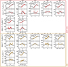 |
Fig. 6. Observed rotation curves (RCs) of the CRISTAL disk sample. The RCs are the fitted line velocity centroids of the position-velocity diagram extracted along the kinematic major axis. The RCs are grouped according to their kinematics types. The black curves are the extracted 1D model (in the same way as data) from the best-fit 3D model cube from DysmalPy. The 3D model cubes are projected and convolved with the beam, which gives rise to the apparent central peak in the velocity dispersion profile and the shallower velocity profiles. The two symmetric grey vertical lines about the dynamical centre indicate the effective radius. The synthesised beam size is shown as the horizontal black line at the top. CRISTAL-05 and 22a belong to Disk, their velocity profiles are shown in Posses et al. (2025) and Telikova et al. (2025), respectively. |
Since for all galaxies, the resolution and S/N of our data cannot provide constraints on many parameters, we leave four parameters free: (i) the baryonic mass log10(Mbary/M⊙), (ii) the disk effective radius Re, disk (kpc), (iii) the enclosed DM fraction fDM(< Re, disk), and (iv) the velocity dispersion σ0 (km s−1). We employ Gaussian priors for log10(Mbary/M⊙), with a standard deviation of 1 dex centred on the sum of the stellar mass reported in Li et al. (2024) and Mitsuhashi et al. (2024) and the molecular gas mass derived in Appendix C. For Re, disk (henceforth Re), we adopted Gaussian priors of standard deviation 1 kpc, centred on the fitted value of Re of the [C II] emission measured in Ikeda et al. (2025). For CRISTAL-10a-E, 12 and 15, the quality of the data was not sufficient to constrain the Re, we fix Re to the [C II]-based radius. The prior range was tailored for each galaxy but generally spans [0, 10] kpc. We assumed flat bounded priors for the intrinsic dispersion σ0 ∈ [20 200] km s−1 and DM fraction, fDM(< Re, disk) ∈ [0, 1]. Finally, we fixed the geometrical parameters i and PA inferred from Eq. (2) and Sect. 3.1, respectively. Other parameters were either tied, such as the disk scale height (through Re) and halo virial mass (through fDM), or fixed. We ran DysmalPy with the emcee sampler, employing 512 walkers and a minimum of 200 burn-in steps followed by 1000 iterations. For all our fits, the final acceptance fraction is between 0.2 and 0.5 (mean = 0.32) and the chain is run for > 10× (mean = 23×) the maximum estimated parameter autocorrelation time (Foreman-Mackey et al. 2013).
We began the first modelling without the bulge component, given that the F444W/NIRCam data show no strong indication of a bulge based on the relatively low Sérsic indices (Appendix B). For some galaxies, we observed a fair level of residuals between the data and the best-fit velocity and dispersion models in the central region, which could be evidence of a concentrated mass distribution deviating from the pure exponential disk profile. We therefore introduced a small, low-mass de Vaucouleurs bulge component with a fixed Sérsic index (nbulge = 4) and an effective radius (Re, b ⩽ 1 kpc).
We iteratively incremented the bulge-to-total ratio B/T in steps of 0.1. For all but 2 cases, a value of B/T = 0.1 led to the best fit in terms of reduced-χ2. For two galaxies, the preferred value is B/T ⩾ 0.3 (CRISTAL-06b, as well as CRISTAL-05 modelled by Posses et al. 2025).
We compare in Fig. 6 the observed and best-fit (projected and beam-smeared) model RCs for the CRISTAL disks. The intrinsic circular velocity profiles Vcirc(R) of the models are shown in Fig. 7, with the maximum radial coverage of the data indicated. Fig. E.1 in Appendix E shows the intrinsic σ0, circular velocity profiles of the DM and the baryonic components. For all systems, except CRISTAL-01b, 07a, 08, 19, 23b, and 23c, we observe a fall-off of circular velocities, indicative of masses dominated by the baryonic components. We will discuss the DM fractions of the samples later in Sect. 7.
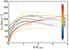 |
Fig. 7. Intrinsic total circular velocity profiles Vcirc(R/Re, disk) of all CRISTAL disks, corrected for beam-smearing and projection effects. Colours in ascending order represent the CRISTAL ID (first column in Table 3). The individual Vcirc(R) of baryons and DM are presented in Figure E.1 in Appendix E. Thin, lighter coloured lines indicate the radial range beyond which the data are not covered. |
We examined the potential dependence of σ0 on the angular resolution relative to the galaxies’ sizes and i. Table 3 lists the ratios of Rout to the beam size (geometric average of the values in Table 1) in terms of half-width-half maximum (beamHWHM). Rout represents the outermost radius at which we can reliably extract velocity and dispersion profiles using the method described in Sect. 3.2. Overall, the kinematics profiles are traced out to ∼1.5–3Re (∼9 Re for CRISTAL-23c), with Rout/beamHWHM ∼ 2–4 (5.5 for CRISTAL-02). Lee et al. (2025) has tested these requirements are sufficient to recover Vrot and σ0 with a large suite of mock galaxies having comparable angular resolution and S/N to the CRISTAL data, provided that the adopted parametric profiles are close to the intrinsic profiles.
We performed Spearman and Kendall rank correlation tests (Fig. 8) to investigate the relationships between σ0–Rout/beamHWHM as well as σ0–i. We do not detect significant correlations in either case (similarly for σ0–Re/beamHWHM). The small sample size, however, would only allow us to detect stronger correlations if present.
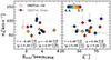 |
Fig. 8. Intrinsic velocity dispersion, σ0, as a function of the number of resolution elements within the outermost measurable radius, Rout, and inclination (i). The Spearman and Kendall rank correlation coefficients (ρ and τ, respectively) do not indicate a significant correlation of σ0 with the inclination and resolution effects, although the uncertainties in both the coefficients and p-value are large. CRISTAL-03, which has Rout/beamHWHM = 1.6 is excluded in the correlation analysis in Sect. 6.2. |
We conservatively exclude the least-resolved CRISTAL-03 in the correlation analysis in Sect. 6.2, which has Rout/beamHWHM = 1.6. For this galaxy, the 5× better angular resolution NIRSpec/JWST data reveal a consistent rotational pattern in Hα (Ren et al., in prep.; Gomez-Espinoza et al., in prep.).
6. Disk turbulence and dynamical support
6.1. Comparison to other samples and redshift trends
To put the CRISTAL disks’ kinematics in the context of dynamical evolution over cosmic time, we present in Fig. 9 the intrinsic dispersion, σ0, and the dynamical support from Vrot/σ0, compared with literature values from local to distant galaxies up to z ≲ 8. The data points are coded according to the MS offset, ΔMS, of the galaxies, and different symbols distinguish measurements based on tracers of atomic, cold molecular, warm, and ionised gas phases.
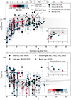 |
Fig. 9. Dynamical evolution of high-z galaxies. Top: Intrinsic velocity dispersion σ0 as a function of redshift for our disk sample (black hexagons with green outline) compared with the literature values (see Appendix D Table D.1). Bottom: Same but for the ratio between rotational velocity and σ0, Vrot/σ0. The solid and dashed black lines are the Übler et al. (2019)’s best-fit relations for galaxies at z < 4, for ionised and cold molecular gas, respectively. Where available, the points are colour-coded by their MS offset, ΔMS, relative to the Speagle et al. (2014) relation, otherwise in grey. The insets show the literature sample (see Table D.2) of the same galaxy with two gas tracers tracing different phases. The insets include the galaxies with large uncertainties, which are omitted in the main plots. The grey shading encloses the corresponding range in σ0 and Vrot/σ0 for Q ∈ [0.6, 2.0]. The definition of the Toomre Q parameter is presented in Sect. 6.3. |
The literature compilation is listed in Appendix D Table D.1. It includes studies of local galaxies and local analogues observed in H I, CO, Hα or [O II], as well as unlensed and lensed galaxies at 0.5 < z < 4 traced by CO, [C I], Hα, [O III] or [C II], and at z ⩾ 4 traced by Hα, CO, [C II], [O III], or [C III]. We only consider the systems classified as disk-like. We exclude those measurements with uncertainties in σ and Vrot greater than 50%, but include all disks in CRISTAL without this cut.
The definition and methodology employed for Vrot and σ0 vary between studies. In cases where Vrot is not available at Re is not available, Vrot is taken as the maximum velocity Vmax or Vrot(2.2Re). For parametric modelling, the profiles adopted for Vrot include arctan and the multi-parameter function from Courteau (1997). The definition of σ also varies across literature; for non-parametric modelling, such as using 3DBarolo (Di Teodoro & Fraternali 2015) or KinMS (Davis et al. 2013, 2017), it would be either the median or the mean of the radial profile; for parametric modelling, which assumed either a constant profile σ(R) = σ0, σ(R) = σ0exp(−R/Rσ) or other functions, we adopt the σ0 or the median in the latter cases, following the choice of the original authors. The literature values are also a mix of data obtained from various observational methods, including IFU, interferometry, and slit spectroscopy. The slit-based method tends to give higher σ values than the other two (Übler et al. 2019). Different CO transitions can also trace gases with various kinematic and spatial properties.
We recalculate ΔMS using the relation of Speagle et al. (2014), extrapolated to the redshift range of the samples. Recent studies of the star-forming MS at z ≳ 5, utilising JWST imaging data, have provided support for this extrapolated relationship (Koprowski et al. 2024; Cole et al. 2025). When available, the stellar mass M⋆ values are taken directly from the literature, which was derived from spectral energy distribution (SED) fitting using various tools and assuming different initial mass functions (IMFs) or decomposition of RC. In cases where M⋆ is not reported, we estimate it from the dynamical and gas mass (M⋆ = Mdyn − Mgas).
In Fig. 9, the literature values of σ0 in ionised and molecular gas tracers are both displaying an overall increasing trend with redshift. For MS galaxies up to z ∼ 4, the trends are well-described by the best-fit relations derived by Übler et al. (2019). Qualitatively, extrapolating these relations matches the evolutionary trend at even higher redshifts for the MS galaxies and agrees well with the CRISTAL values. On the other hand, some starburst galaxies observed with [C II] at similar epochs lie below the extrapolated relationships.
Sample selection differences between studies could partly explain the large spread in σ0 (and Vrot/σ0). As extensively discussed by Wisnioski et al. (2025), the interpretation of the dispersion should also consider the different ISM phases probed by the various kinematic tracers and, relatedly, the varying contributions of different gas phases to the [C II] line emission as a function of ΣSFR and other properties (e.g. Cormier et al. 2019; Wolfire et al. 2022; Ikeda et al. 2025). To better understand the potential dependence on ISM phases, it is essential to study the same object using multiple tracers; currently, this has only been done for a limited number of samples (Table D.2), as highlighted in the insets of Fig. 9.
Compared to unlensed MS SFGs observed with [C II] at similar epochs, CRISTAL disks have comparable values of σ0 within uncertainties, with a median difference of 11 km s−1, and a lower Vrot/σ0 by 0.8 in median. This is possibly because CRISTAL disks are less massive in M⋆ than the literature samples by an average of 0.15 dex. Given the mass-dependence of Vrot/σ in simulations that span a wider dynamic range (e.g. Dekel et al. 2020; Kohandel et al. 2024) than allowed by our data, the lower mass of our sample may explain the lower Vrot/σ0 values. When compared with the same population observed in ionised gas, now possible thanks to JWST, CRISTAL disks are in very good agreement with the ‘gold’ sample in Danhaive et al. (2025), with median differences of only ∼2% in σ0 and ∼10% in Vrot(Re)/σ0.
On the other hand, compared with the lensed samples, CRISTAL disks have higher σ0, by 34 km s−1 in median, and significantly lower Vrot/σ0 by −6. In particular, the lensed samples tend to be starburst galaxies, and have smaller sizes (with Re typically ≲1.5 kpc, see also Fig. 1) that are ∼50% and ∼70% smaller than the unlensed galaxies and CRISTAL disks, respectively. The starburst and compact nature of these galaxies suggests that they have experienced a distinct assembly history (Stach et al. 2018; Hayward et al. 2021), differing from that of the more typical galaxy populations in CRISTAL.
6.2. Trends with galaxy properties
We explored any existing trends with the galaxy properties, including molecular gas mass fraction (fmolgas), stellar mass (M⋆), MS offset (ΔMS), SFR surface density (ΣSFR), and molecular gas mass (Mgas). Fig. 10 plots the derived σ0 and Vrot/σ0 as a function of these properties for the CRISTAL disk sample. We quantify the correlations by computing Spearman’s ρ and Kendall’s τ, and their p-values to assess the significance of any possible correlations. The resulting coefficients and the p-values with confidence intervals are annotated in Fig. 10.
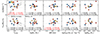 |
Fig. 10. Intrinsic velocity dispersion (σ0) and the ratio of rotation velocity at the effective radius (Vrot(Re)) to intrinsic velocity dispersion (σ0) as a function of five galaxy properties: molecular gas fraction (fmolgas), stellar mass (log(M⋆/M⊙)), offset from the main sequence (ΔMS), star formation rate surface density (ΣSFR), and molecular gas mass (log(Mgas/M⊙)). The dashed and solid grey curves in the first column are the predicted trends based on Equation (3) with Q fixed at Qcrit = 0.67, with a = 1 and a= |

For σ0, the strongest correlation observed is with fmolgas. The Vrot/σ0 value appears to be primarily correlated with ΔMS. No other obvious trend was detected with the other galaxy properties. The dependence of σ0 with fmolgas is in line with expectations for marginally stable, gas-rich disks as discussed in Sect. 6.1. The trend between Vrot/σ0 and ΔMS may reflect an underlying dependence on Σbar (see also the right panel of Fig. 1). However, although the correlation coefficient ρ between Vrot/σ0 and Σbar is ∼0.5, the large accompanying p-value suggests that more precise size measurements are required to confirm this relationship. Clearly, the CRISTAL disk sample is small, and only the strongest correlations can be discerned. Future larger samples of near MS SFGs at z ∼ 4–6 will be important to strengthen the results, such as the literature compilation efforts by Wisnioski et al. (2025).
6.3. Turbulence in the framework of marginally Toomre-stable disks
The observed evolutionary trend of σ0 and Vrot/σ0 discussed above has been attributed to the increasing gas fraction at higher redshifts (e.g. Tacconi et al. 2010, 2020), as predicted by the Toomre theory. The correlation of σ0 with fmolgas for the CRISTAL disks discussed above is also in line with expectations for marginally stable gas-rich disks. In this framework, thestability of the disks against fragmentation and local gravitational collapse is directly linked to the level of turbulence in the ISM. Turbulence is driven by both ex-situ, such as accretion from the cosmic web, and in-situ, including radial flows and clump migration, which release gravitational potential energy. This creates a self-regulating cycle that maintains the disk in a state of marginal stability. Following Eq. (3) in Genzel et al. (2014) (see also, Übler et al. 2019; Genzel et al. 2011, 2023; Liu et al. 2023), the classical Toomre (1964) parameter Q can be formulated as
 (3)
(3)
where the epicyclic frequency is κ =  and Ω = Vrot/R. The constant a depends on the rotational structure of the disk: a =
  for Keplerian-like rotation and a =
  for a disk with constant rotational velocity. For a quasi-stable thick gas disk, Qcrit = 0.67 (e.g. Behrendt et al. 2015). The two panels in the first column of Fig. 10 plot the predicted trends of σ(fgas) and Vrot/σ(fgas) based on Eq. (3) with Q = Qcrit and a =
  , taking into account that some RCs show a drop-off. Overall, there is a good match between the predicted trend and the CRISTAL values.
Specifically, taking the median values of CRISTAL disks, σ0/vc = 70/200 = 0.4 and fmolgas ∼ 0.5. The corresponding values of Qgas is then 0.6, and the entire sample has Q in the range [0.4, 2.0], indicating that the CRISTAL disks are, on average, marginally gravitationally stable. The Q values are broadly similar to the results of Übler et al. (2019) for their z ∼ 1–3 samples. The similar Toomre Q values inferred for MS SFGs from z ∼ 5 to z ∼ 1 in MS SFGs suggest that this galaxy population has grown in a marginally stable and self-regulating manner for at least 5 billion years of cosmic time.
From a broader evolutionary perspective based on the Toomre theory for gas-rich disks, the observed trends from the literature, combined with CRISTAL, are in remarkably good agreement. The grey bands in both panels of Fig. 9 show the prediction in the Toomre framework for the evolution of dispersion for log(M⋆/M⊙) = 10.0 galaxies with Qcrit ∈ [0.4, 2.0] and vc = 200 km s−1. These values are appropriate for the CRISTAL disk sample (and differ from more massive samples studied at lower redshifts, e.g. Wisnioski et al. 2015). The gas fraction fmolgas adopted evolves according to the scaling relation in Tacconi et al. (2020) which is a function of stellar mass, SFR, and size. The SFR and size evolution with redshift is determined from the Speagle et al. (2014) MS relation and van der Wel et al. (2014) mass-size relation. CRISTAL galaxies have fmolgas ∼ 51%, consistent with the expected value from Tacconi et al. (2020)’s relation at z = 5 for M⋆ = 1010 M⊙, which is ∼53% (see discussions in Appendix C).
6.4. Drivers of the gas turbulence
To explore the relative contribution of star formation- versus gravitational instability-driven turbulence in CRISTAL disks, we compare our results with the analytic model of Krumholz et al. (2018). This model combines stellar feedback and gravitational processes to drive turbulence, incorporating prescriptions for star formation, stellar feedback, and gravitational instabilities into a unified ‘transport+feedback’ framework. In the model, gas is in vertical hydrostatic equilibrium and energy equilibrium, with energy losses through turbulence decay balanced by energy input from stellar feedback and the release of gravitational energy via mass transport through the disk. Based on the model, there is a critical value of gas velocity dispersion (σg), σsf, at which the amount of turbulence can be sustained by star formation alone, without the need for gravitational instability or radial transport. In such a case, σg is related to σsf by (Eq. (39) in Krumholz et al. 2018)
![Mathematical equation: $$ \begin{aligned} \sigma _{\rm g}=\sigma _{\rm sf}&\equiv \frac{4f_{\rm SF}\epsilon _{\rm ff}}{\sqrt{3f_{g,P}}\pi \eta \phi _{\rm mp}\phi _Q\phi _{\rm nt}^{3/2}}\left\langle \frac{p_*}{m_*}\right\rangle \nonumber \\&\cdot \mathrm{max}\left[1,\,\sqrt{\frac{3f_{g,P}}{8(1+\beta )}}\frac{Q_{\rm min}\phi _{\rm mp}}{4f_{g,Q}\epsilon _{\rm ff}}\frac{t_{\rm orb}}{t_{\rm sf,max}}\right]. \end{aligned} $$](/articles/aa/full_html/2025/09/aa55362-25/aa55362-25-eq176.gif) (4)
(4)
ollowing Table 3 in Krumholz et al. (2018) for high-z galaxies, the fraction of ISM in the star-forming molecular phase, fSF, is set to 1.0; tSF, max = 2 Gyr; the fractional contribution of gas to the mid-plane pressure and Q, fg, P and fg, Q, respectively, are both assumed to be 0.7; the slope index of the RC, β = dlnvϕ/dlnr, is set to 0.0 (i.e., flat), in which vϕ is the circular velocity Vcirc; the Toomre parameter, Q, is fixed at 1, following the fiducial value. The orbital period torb = 2πr/Vcirc ∈ [30, 120] Myr, and is adjusted to the values of our sample. The other values that we adopt are listed in Table F.1 in Appendix F. The σg from Eq. (4) is therefore ∼10 km s−1. Dispersion much larger than this critical value (≳20 km s−1) requires gravitational instability or radial mass transport for moderate SFR.
In the ‘transport+feedback’ model, the star formation rate surface density ΣSFR and the gas velocity dispersion σg can be related following (Eq. (59) in Krumholz et al. 2018) as
![Mathematical equation: $$ \begin{aligned} \Sigma _{\rm SFR}&= f_{\rm SF}\frac{\sqrt{8(1+\beta )}f_{g,Q}}{GQ} \frac{\sigma _g}{t^2_{\rm orb}} \nonumber \\&\cdot \text{ max} \left[\frac{8\epsilon _{\rm ff} f_{g,Q}}{Q} \sqrt{\frac{2(1+\beta )}{3f_{g,P}\phi _{\rm mp}}}, \frac{t_{\rm orb}}{t_{\rm SF, max}} \right], \end{aligned} $$](/articles/aa/full_html/2025/09/aa55362-25/aa55362-25-eq177.gif) (5)
(5)
while for the ‘feedback-only’ (fixed Q) model (Eq. (61) in Krumholz et al. 2018), we have
 (6)
(6)
In Fig. 11, we show the σ0–ΣSFR3 measurements of CRISTAL disks, compared with the ‘transport+feedback’ and ‘feedback only’ model of Krumholz et al. (2018). For reference, we also compare σ0 and SFR in Appendix F. Overall, our results are broadly consistent with the ‘feedback+transport’ model of Krumholz et al. (2018), which suggests that the high-velocity dispersion of normal SFGs can be predominantly attributed to the release of gravitational energy from mass transport across the disk.
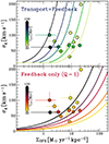 |
Fig. 11. σ0 vs ΣSFR of CRISTAL disks compared with analytical models from Krumholz et al. (2018). The solid lines in the upper panel show the σ0 values predicted from the Transport+Feedback model with orbital period torb = [30, 120] Myr. Similarly, for the lower panel, but for the ‘Feedback-only’ model. The results are broadly consistent with the ‘feedback+transport’ model, suggesting that the elevated velocity dispersion of normal star-forming galaxies at this epoch requires additional gravitational energy from mass transport across the disk. |
This result differs from some previous studies at similar epochs, which found that star formation feedback alone can sustain the observed dispersion in starburst-like galaxies (e.g. Roman-Oliveira et al. 2023; Rowland et al. 2024). However, our analysis of CRISTAL MS disks, characterised by modest star formation activity, indicates that a different dominant mechanism drives turbulence in the ISM of MS SFGs.
The result is nevertheless consistent with the weak correlation of σ with global or local SFR (ΣSFR) of our sample as shown in Sect. 6.2. Such a weak correlation is also found in Genzel et al. (2011), Johnson et al. (2018) and Übler et al. (2019) for cosmic noon galaxies (after redshift normalisation), and in the nearby universe (e.g. Elmegreen et al. 2022). This is also in agreement with the theoretical works (e.g. Shetty & Ostriker 2012; Kim & Ostriker 2018), which have derived a weak dependence of gas velocity dispersion on the supernova explosion rate.
We note, however, that for CRISTAL-05 with its relatively low σ0 ≈ 31 km s−1 and ΣSFR = 8.5 M⊙ yr−1 kpc−2 (SFR = 68 M⊙ yr−1), the stellar feedback-only model would better match the observed values of σ0 and ΣSFR (and SFR), suggesting that different mechanisms among the disk sample may contribute to varying degrees of the observed velocity dispersion, as seen also in simulations (e.g. Jiménez et al. 2023). Additionally, spatial variation of different mechanisms within a single galaxy is also possible, but the resolution of our data is currently insufficient to reveal such variation conclusively. In the future, higher resolution observations of kinematics and SFR maps would enable to test more directly the coupling (or lack thereof) between σ0 and stellar feedback. Other simulation works also show that stellar feedback can sustain higher dispersions compared to the Krumholz et al. 2018’s analytical treatment (Gatto et al. 2015; Orr et al. 2020; Rathjen et al. 2023). The relative contribution of stellar feedback versus gas transport depends on halo mass and redshift, in which gas transport plays a more dominant role in the high redshift systems (Ginzburg et al. 2022).
7. Exploration of galactic DM fraction and mass budget
On the galactic scale, CRISTAL disks tend to be baryonic-dominated, with low fDM at Re (Table 3), having a median value of 18% (mean = 27%), comparable to or less than maximal disks (fDM ≔ 28% van Albada et al. 1985), albeit with significant scatter among the samples that span a wider range from a few % to ∼60%. In comparison, the Galaxy’s fDM(Re) = 0.38 ± 0.1 (Bovy & Rix 2013; Bland-Hawthorn & Gerhard 2016).
The radial profiles of fDM of CRISTAL disks are shown in Fig. E.1, which is defined in DysmalPy as4
 (7)
(7)
We observe a tentative inverse relationship between fDM(Re) and circular velocity (Vcirc) in Fig. 12, which is pressure-support corrected (Eq. (1)), and similarly for the baryonic surface density Σbary based on the values in Tables 1 and 2. This trend is similar to that observed in Nestor Shachar et al. (2023) for cosmic noon MS SFGs. Such an inverse correlation is well-established for local SFGs, where the most DM-dominated disks are those with low Σbary and Vcirc (e.g. Martinsson et al. 2013a,b; Courteau & Dutton 2015, and references therein). We also compare our results to Wuyts et al. (2016), who derived fDM at the inner disk by subtracting the sum of stellar and gas masses from the dynamical mass obtained from RCs of 240 galaxies, assuming fbary = Mbary/Mdyn = 1 − fDM. We find that most of the CRISTAL disks follow the Wuyts et al. (2016) relation on the Σbary–fDM plane, except for CRISTAL-23b and 23c, which are both disk-like galaxies in an interacting system.
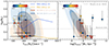 |
Fig. 12. DM fraction, fDM, as a function of the circular velocity at the effective radius, Vcirc(Re) (left), and baryonic surface density, Σbary (right). The yellow and blue curves show the TNG100 (without adiabatic contraction) relations at z = 0 and z = 2 (Lovell et al. 2018), respectively. The pale blue and red shadings are measurements from RC100 at z < 1.2 and z < 2.5, respectively (Nestor Shachar et al. 2023). The thick grey dashed curve is the best-fit relation of z ∼ 2 star-forming galaxies from Wuyts et al. (2016). The CRISTAL sample statistics suggest a tentative anti-correlation with fDM(Re) and Σbary, although individual galaxy uncertainties are limited by the data depth. The horizontal dashed line denotes fDM for a maximal disk fDM ≔ 28% (van Albada et al. 1985). In the right panel, the two symbols plotted with only limit arrows represent CRISTAL-10a-E (upper limit) and CRISTAL-06b (lower limit). The stellar mass is only for CRISTAL-10a as a whole, which includes CRISTAL-10a-E, while no gas mass is available for CRISTAL-06b. |
The low fDM(Re) of our sample is broadly consistent with the general trend of decreasing DM fraction towards higher redshifts. Fig. 13 shows the median fDM(Re) of our sample aligns with the extrapolated trend toward higher redshift from Nestor Shachar et al. (2023) and Wuyts et al. (2016), when considering a sample matched in Mbary and ΔMS. Both fDM are below the expectations from the TNG100 simulation from Lovell et al. (2018). This could be due to the insufficient physical resolution of large-scale cosmological simulations to resolve sub-galactic processes (Übler et al. 2021) and the effect of adiabatic contraction (Blumenthal et al. 1986). The possible drivers of DM deficit in MS SFGs have been discussed thoroughly by, e.g. Genzel et al. (2020) and Nestor Shachar et al. (2023). It is potentially linked to kinetic heating due to the efficient transport of baryons to central regions in gas-rich systems (e.g. El-Zant et al. 2001), and/or strong feedback processes redistributing DM to larger radii (e.g. Freundlich et al. 2020). One example is CRISTAL-02, which has fDM(Re) < 0.1 and drives a vigorous outflow detected in [C II] (Davies et al. 2025).
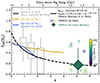 |
Fig. 13. DM fraction at effective radius (fDM(Re)) as a function of redshift. The fDM(Re) of individual CRISTAL disks (4 < z < 6) are represented by small diamonds, colour-coded by their Vcirc(Re). For comparison, we include lower redshift studies around z = 2 from Wuyts et al. (2016) (grey box-and-whisker) and the best-fit relation to the RC100 data set (Nestor Shachar et al. 2023) (black solid line for the redshift range covered and dashed line for the extrapolated range). For both observational studies, we consider only SFGs on the MS and the baryonic mass Mbary matched within 0.3 dex of the CRISTAL disks. The new best-fit relation to RC100, using the Mbary-matched sample, is shown in the legend. The trends predicted from the TNG100 simulation for M* = 1010 M⊙ and M* = 1011 M⊙ are shown in yellow and blue, respectively (Lovell et al. 2018). Overall, the CRISTAL disks tend to be baryon-dominated on galactic scales, with a median DM fraction of ∼18% (large green diamond) that is tentatively consistent with the extrapolated relation based on RC100. However, there is a significant scatter in the values among the sample, partly driven by the scattered distributions of circular velocity Vcirc(Re) (and Σbary) shown in Figure 12. |
The widely scattered distribution in Fig. 13 with large errors associated with individual galaxies prevents a definite conclusion on the physical origin of this distribution. We investigated whether the inhomogeneous radial coverage of the RCs (Fig. 7) could systematically drive up the fDM(Re) for galaxies with limited radial coverage. However, we do not find a straightforward one-to-one correspondence between fDM(Re) and the ratio of Rout/Re (Kendall’s  ,
,  ).
).
We emphasise that fDM is measured at the effective radius, and we lack constraints on the DM distribution on the halo scale (≫Re) with our current data, except for the very compact CRISTAL-23c. Extrapolating the DM mass from the inner disk to the virial scale with an NFW distribution would result in an unphysically large baryon fraction larger than the cosmic baryon fraction (Genzel et al. 2017). As discussed in Sect. 5.1, the intrinsic, circular velocities would also depend on the assumption of the pressure support corrections, which would explain the differences found in the literature (cf. Sharma et al. 2021 with, e.g. Genzel et al. 2020; Price et al. 2021 and Nestor Shachar et al. 2023). If we were to assume a non-constant σ, such as an exponential decline, for the pressure support correction, rather than using Eq. (1), the correction to Vrot would be even larger (Eq. (12) in Price et al. 2022), leading to a more steeply declining Vcirc, which would further exacerbate the discrepancies between our observations and simulations.
Although we have adopted the NFW profile for the DM profile, the fDM(< Re) results for the sample change less than 10% (in terms of absolute difference) for alternative DM mass profile assumption, such as the two-power halo (2PH) profile (Binney & Tremaine 2008) with a variable inner slope. Improved constraints on the DM fraction in the future would benefit from deeper observations of individual galaxies and/or kinematic stacking analysis (e.g. Lang et al. 2017; Tiley et al. 2019).
8. Nature of Non-Disks
The origin of the kinematic perturbations in the Non-Disk subset of the sample could arise from galaxy interactions and mergers. Most Non-Disks, except CRISTAL-21, 24 and 25, have visible companions already in the HST and/or JWST images alone, and the one classified as Non-Disk is, in most cases, the less luminous and less massive for those with available mass measurement. The higher non-disk fraction among the CRISTAL kinematic sample compared to samples of typical MS SFGs at lower redshift may not be surprising in view of the increase in merger rates with redshift from both observational work (Duncan et al. 2019; Romano et al. 2021; Duan et al. 2025; Puskás et al. 2025; Shibuya et al. 2025) and numerical simulations (Rodriguez-Gomez et al. 2015; Pillepich et al. 2019; O’Leary et al. 2021). It will be interesting to investigate the environment of the galaxies in greater detail in a future study, allowing us to quantify, for instance, the interaction strengths from neighbouring systems. More complete redshift identification around the CRISTAL galaxies will be necessary for that purpose.
9. Summary and outlook
In this work, we present a kinematic study of a sample of MS SFGs at redshift 4 < z < 6 from the ALMA-CRISTAL programme. The angular resolution of the sensitive [C II] ALMA observations enables the characterisation of the kinematics of galaxies at a scale of ∼1 kpc. We classified the galaxies primarily based on their kinematic features traced by [C II] using a variety of methods that have been applied in lower redshift studies, supplemented by morphological information from HST and JWST imaging (Sect. 3). We found that 50 ± 9% of the galaxies in our sample are disk-dominated (Sect. 4), with over half of them located in systems of multiple components, which differs from the more isolated environment of lower redshift disks. We fitted the kinematics of the disks using fully forward-modelled 3D kinematic models (Sect. 5). Our kinematic modelling reveals the following important properties of the CRISTAL MS disks:
-
They have a high contribution of turbulence relative to rotational support, with a median disk velocity dispersion of ∼70 km s−1 and Vrot(Re)/σ0 of ∼2 (Sect. 6.1).
-
Their high-velocity dispersions are consistent with the predicted evolution based on Toomre theory and the extrapolated evolutionary trends based on detailed studies of cosmic noon to lower redshift galaxies (Sect. 6.1).
-
Their tentative correlation between gas mass and velocity dispersion provides hints that the high dispersion is sustained by gravitational instability, but it is unclear whether this is a local or global phenomenon (Sect. 6.2).
-
They tend to have a low DM fraction, with a median of fDM(< Re) ≈ 18%, while spanning a significant range from ∼5% to ∼60%; the median value is in broad agreement with the extrapolated trend based on studies of lower redshifts, albeit with large scatter (Sect. 7).
The deep, high-resolution ALMA observations of [C II]158 μm line emission from the CRISTAL programme allowed us to carry out a first systematic census of the kinematics of typical MS star-forming galaxies at z ∼ 4–6. The brightness of [C II] along with its sensitivity to the multi-phase ISM make it an ideal probe of the gas motions (among other properties) over a large extent of galaxies encompassing cold molecular gas, ionised, and photodissociation regions. These properties facilitate measurements reaching the outskirts of galaxies. As observations of rest-optical line emission originating from the warm ionised gas phase become available from JWST IFU follow-up of CRISTAL targets, direct comparisons will become possible. This will be important especially with regard to the issue of gas turbulence. As discussed in this work (Sect. 6) and in the literature (e.g. Girard et al. 2021; Ejdetjärn et al. 2022; Kohandel et al. 2024; Wisnioski et al. 2025), it would greatly benefit from measurements in multiple tracers for the same objects. Another outlook enabled by CRISTAL-ALMA and JWST-IFU synergies is the connection between spatial variations in terms of the gas-phase metallicity and kinematics, which will be the subject of a forthcoming study.
Except for CRISTAL-19, in which the higher resolution Briggs-weighted (robust = 0.5) cubes have sufficient S/N. There is, however, no significant difference in the kinematics modelling results between the natural-weighted and Briggs-weighted cubes.
For CRISTAL-23c in which the ΣSFR is not available, we adopt the ΣSFR, IR from Béthermin et al. (2023) as a lower limit, although the contribution from unobscured star formation is not significant.
We note that in our analysis, fDM at Re, disk is a free parameter – by instead calculating the total halo mass given the specified baryonic mass distribution and fDM(Re, disk), the full fDM radial profile for each galaxy is then computed given the best-fit parameters (Mbar, Re, disk, fDM enclosed within Re, and σ0).
Data from Very Large Array (VLA) observations of CO(2-1) are available for CRISTAL-22 (HZ10) and CRISTAL-02 (LBG-1).
This temperature is luminosity-weighted, as the mass-weighted temperature is not available, see Scoville et al. (2016) and Scoville et al. (2017) for the discussion of the resulting difference in the dust mass between the two temperatures.
β is frequency-dependent but is not constrained by our data.
Tacconi et al. (2020) assumes lower αCO and XCO than Scoville et al. (2016)’s.
Acknowledgments
We thank the anonymous referee for the constructive feedback which improves the clarity of the work. L.L.L. is thankful for the stimulating discussions with M. Bureau, Q. Fei, S. Pastras, W. Maciejewski and E. Wisnioski at the various stages of this work. L.L.L. thanks A. Nestor for providing the data tables for Fig. 12. N.M.F.S. and J.C. acknowledge financial support from the European Research Council (ERC) Advanced Grant under the European Union’s (EU’s) Horizon Europe research and innovation programme (grant agreement AdG GALPHYS, No. 101055023). H.Ü. acknowledges funding by the EU (ERC APEX, 101164796). Views and opinions expressed are, however, those of the author(s) only and do not necessarily reflect those of the EU or the ERC. Neither the EU nor the granting authority can be held responsible for them. R.H-C. thanks the Max Planck Society for support under the Partner Group project ‘The Baryon Cycle in Galaxies’ between the Max Planck for Extraterrestrial Physics and the Universidad de Concepción. M.A. and R.H-C. also gratefully acknowledge financial support from ANID – MILENIO – NCN2024_112. M.A., R.J.A., R.H-C., M.S. and K. Telikova acknowledge support from ANID BASAL FB210003. R.J.A. was supported by FONDECYT grant number 1231718. R.B. acknowledges support from an STFC Ernest Rutherford Fellowship [grant number ST/T003596/1]. R.L.D. is supported by the Australian Research Council through the Discovery Early Career Researcher Award (DECRA) Fellowship DE240100136 funded by the Australian Government. T.D-S. acknowledges the research project was supported by the Hellenic Foundation for Research and Innovation (HFRI) under the ‘2nd Call for HFRI Research Projects to support Faculty Members & Researchers’ (Project Number: 03382) I.D.L. acknowledges funding from the ERC under the EU’s Horizon 2020 research and innovation program DustOrigin (ERC-2019-StG-851622) and from the Flemish Fund for Scientific Research (FWO-Vlaanderen) through the research project G0A1523N. R.I. is supported by Grants-in-Aid for Japan Society for the Promotion of Science (JSPS) Fellows (KAKENHI Grant Number 23KJ1006). T.N. acknowledges the support of the Deutsche Forschungsgemeinschaft (DFG, German Research Foundation) under Germany’s Excellence Strategy – EXC-2094 – 390783311 of the DFG Cluster of Excellence ‘ORIGINS’. M.S. was financially supported by Becas-ANID scholarship #21221511. K. Tadaki acknowledges support from JSPS KAKENHI Grant No. 23K03466. K. Telikova was supported by ALMA ANID grant number 31220026. V.V. acknowledges support from the ALMA-ANID Postdoctoral Fellowship under the award ASTRO21-0062. This paper makes use of the following ALMA data: ADS/JAO.ALMA#2021.1.00280.L, 2017.1.00428.L, 2012.1.00523.S, 2018.1.01359.S, 2019.1.01075.S. ALMA is a partnership of ESO (representing its member states), NSF (USA) and NINS (Japan), together with NRC (Canada), NSC and ASIAA (Taiwan), and KASI (Republic of Korea), in cooperation with the Republic of Chile. The Joint ALMA Observatory is operated by ESO, AUI/NRAO and NAOJ. This work is based in part on observations made with the NASA/ESA/CSA James Webb Space Telescope and NASA/ESA Hubble Space Telescope. The data were obtained from the Mikulski Archive for Space Telescopes (MAST) at the Space Telescope Science Institute, which is operated by the Association of Universities for Research in Astronomy, Inc., under NASA contract NAS 5-03127 for JWST and NAS 5–26555 for HST. The specific observations analysed can be accessed via 10.17909/2gpc-vd24. Support to MAST for these data is provided by the NASA Office of Space Science via grant NAG5–7584 and by other grants and contracts. Some of the data products presented herein were retrieved from the Dawn JWST Archive (DJA). DJA is an initiative of the Cosmic Dawn Center (DAWN), which is funded by the Danish National Research Foundation under grant DNRF140. This work made use of the following Python packages: Astropy (Astropy Collaboration 2022), corner (Foreman-Mackey 2016), DysmalPy (Davies et al. 2004a,b, 2011; Cresci et al. 2009; Wuyts et al. 2016; Lang et al. 2017; Price et al. 2021; Lee et al. 2025), emcee (Foreman-Mackey et al. 2013), Imfit (Erwin 2015), Matplotlib (Hunter 2007), Numpy (Harris et al. 2020), pymccorrelation (Curran 2014; Privon et al. 2020), Trilogy (Coe et al. 2012), and Scipy (Virtanen et al. 2020).
References
- Amvrosiadis, A., Lange, S., Nightingale, J. W., et al. 2025, MNRAS, 537, 1163 [Google Scholar]
- Astropy Collaboration (Price-Whelan, A. M., et al.) 2022, ApJ, 935, 167 [NASA ADS] [CrossRef] [Google Scholar]
- Barišić, I., Jones, T., Mortensen, K., et al. 2025, ApJ, 983, 139 [Google Scholar]
- Beckers, J. M. 1982, Opt. Acta, 29, 361 [NASA ADS] [CrossRef] [Google Scholar]
- Behrendt, M., Burkert, A., & Schartmann, M. 2015, MNRAS, 448, 1007 [NASA ADS] [CrossRef] [Google Scholar]
- Béthermin, M., Daddi, E., Magdis, G., et al. 2015, A&A, 573, A113 [Google Scholar]
- Béthermin, M., Wu, H.-Y., Lagache, G., et al. 2017, A&A, 607, A89 [Google Scholar]
- Béthermin, M., Fudamoto, Y., Ginolfi, M., et al. 2020, A&A, 643, A2 [Google Scholar]
- Béthermin, M., Accard, C., Guillaume, C., et al. 2023, A&A, 680, L8 [NASA ADS] [CrossRef] [EDP Sciences] [Google Scholar]
- Binney, J., & Tremaine, S. 2008, Galactic Dynamics, 2nd edn. (Princeton University Press) [Google Scholar]
- Birkin, J. E., Puglisi, A., Swinbank, A. M., et al. 2024, MNRAS, 531, 61 [NASA ADS] [CrossRef] [Google Scholar]
- Birkin, J. E., Spilker, J. S., Herrera-Camus, R., et al. 2025, ApJ, 985, 243 [Google Scholar]
- Bland-Hawthorn, J., & Gerhard, O. 2016, ARA&A, 54, 529 [Google Scholar]
- Blumenthal, G. R., Faber, S. M., Flores, R., & Primack, J. R. 1986, ApJ, 301, 27 [Google Scholar]
- Bouché, N. F., Bera, S., Krajnović, D., et al. 2022, A&A, 658, A76 [NASA ADS] [CrossRef] [EDP Sciences] [Google Scholar]
- Bouwens, R. J., Smit, R., Schouws, S., et al. 2022, ApJ, 931, 160 [NASA ADS] [CrossRef] [Google Scholar]
- Bovy, J., & Rix, H.-W. 2013, ApJ, 779, 115 [Google Scholar]
- Burkert, A., Genzel, R., Bouché, N., et al. 2010, ApJ, 725, 2324 [Google Scholar]
- CASA Team, Bean, B., Bhatnagar, S., et al. 2022, PASP, 134, 114501 [NASA ADS] [CrossRef] [Google Scholar]
- Cathey, J., Gonzalez, A. H., Lower, S., et al. 2024, ApJ, 967, 11 [NASA ADS] [CrossRef] [Google Scholar]
- Christy, J. W., Wellnitz, D. D., & Currie, D. G. 1981, Lowell Obs. Bull., 9, 28 [Google Scholar]
- Clark, P. C., Glover, S. C. O., Ragan, S. E., & Duarte-Cabral, A. 2019, MNRAS, 486, 4622 [Google Scholar]
- Coe, D., Umetsu, K., Zitrin, A., et al. 2012, ApJ, 757, 22 [NASA ADS] [CrossRef] [Google Scholar]
- Cole, J. W., Papovich, C., Finkelstein, S. L., et al. 2025, ApJ, 979, 193 [Google Scholar]
- Condon, J. J., Cotton, W. D., Greisen, E. W., et al. 1998, AJ, 115, 1693 [Google Scholar]
- Cormier, D., Abel, N. P., Hony, S., et al. 2019, A&A, 626, A23 [NASA ADS] [CrossRef] [EDP Sciences] [Google Scholar]
- Costantin, L., Gillman, S., Boogaard, L. A., et al. 2025, A&A, 699, A360 [NASA ADS] [CrossRef] [EDP Sciences] [Google Scholar]
- Courteau, S. 1997, AJ, 114, 2402 [Google Scholar]
- Courteau, S., & Dutton, A. A. 2015, ApJ, 801, L20 [Google Scholar]
- Cresci, G., Hicks, E. K. S., Genzel, R., et al. 2009, ApJ, 697, 115 [Google Scholar]
- Curran, P. A. 2014, arXiv e-prints [arXiv:1411.3816] [Google Scholar]
- Dalcanton, J. J., & Stilp, A. M. 2010, ApJ, 721, 547 [NASA ADS] [CrossRef] [Google Scholar]
- Danhaive, A. L., Tacchella, S., Übler, H., et al. 2025, MNRAS, submitted [arXiv:2503.21863] [Google Scholar]
- Davies, R. I., Tacconi, L. J., & Genzel, R. 2004a, ApJ, 602, 148 [NASA ADS] [CrossRef] [Google Scholar]
- Davies, R. I., Tacconi, L. J., & Genzel, R. 2004b, ApJ, 613, 781 [NASA ADS] [CrossRef] [Google Scholar]
- Davies, R., Förster Schreiber, N. M., Cresci, G., et al. 2011, ApJ, 741, 69 [NASA ADS] [CrossRef] [Google Scholar]
- Davies, R. L., Fisher, D. B., Herrera-Camus, R., et al. 2025, Nat. Astron., submitted [Google Scholar]
- Davis, T. A., Alatalo, K., Bureau, M., et al. 2013, MNRAS, 429, 534 [Google Scholar]
- Davis, T. A., Bureau, M., Onishi, K., et al. 2017, MNRAS, 468, 4675 [NASA ADS] [CrossRef] [Google Scholar]
- de Blok, W. J. G., Healy, J., Maccagni, F. M., et al. 2024, A&A, 688, A109 [NASA ADS] [CrossRef] [EDP Sciences] [Google Scholar]
- de Graaff, A., Rix, H.-W., Carniani, S., et al. 2024, A&A, 684, A87 [NASA ADS] [CrossRef] [EDP Sciences] [Google Scholar]
- Dekel, A., & Burkert, A. 2014, MNRAS, 438, 1870 [Google Scholar]
- Dekel, A., Birnboim, Y., Engel, G., et al. 2009, Nature, 457, 451 [Google Scholar]
- Dekel, A., Ginzburg, O., Jiang, F., et al. 2020, MNRAS, 493, 4126 [CrossRef] [Google Scholar]
- Dessauges-Zavadsky, M., Ginolfi, M., Pozzi, F., et al. 2020, A&A, 643, A5 [NASA ADS] [CrossRef] [EDP Sciences] [Google Scholar]
- Devereaux, T., Cassata, P., Ibar, E., et al. 2024, A&A, 686, A156 [NASA ADS] [CrossRef] [EDP Sciences] [Google Scholar]
- Di Teodoro, E. M., & Fraternali, F. 2015, MNRAS, 451, 3021 [Google Scholar]
- Di Teodoro, E. M., Fraternali, F., & Miller, S. H. 2016, A&A, 594, A77 [NASA ADS] [CrossRef] [EDP Sciences] [Google Scholar]
- Duan, Q., Conselice, C. J., Li, Q., et al. 2025, MNRAS, 540, 774 [Google Scholar]
- Duncan, K., Conselice, C. J., Mundy, C., et al. 2019, ApJ, 876, 110 [NASA ADS] [CrossRef] [Google Scholar]
- Dutton, A. A., & Macciò, A. V. 2014, MNRAS, 441, 3359 [Google Scholar]
- Eisenhauer, F., Tecza, M., Thatte, N., et al. 2003, Messenger, 113, 17 [Google Scholar]
- Ejdetjärn, T., Agertz, O., Östlin, G., Renaud, F., & Romeo, A. B. 2022, MNRAS, 514, 480 [CrossRef] [Google Scholar]
- Elmegreen, B. G., Martinez, Z., & Hunter, D. A. 2022, ApJ, 928, 143 [NASA ADS] [CrossRef] [Google Scholar]
- El-Zant, A., Shlosman, I., & Hoffman, Y. 2001, ApJ, 560, 636 [NASA ADS] [CrossRef] [Google Scholar]
- Epinat, B., Amram, P., & Marcelin, M. 2008, MNRAS, 390, 466 [NASA ADS] [Google Scholar]
- Epinat, B., Contini, T., Le Fèvre, O., et al. 2009, A&A, 504, 789 [NASA ADS] [CrossRef] [EDP Sciences] [Google Scholar]
- Erwin, P. 2015, ApJ, 799, 226 [Google Scholar]
- Faisst, A. L., Schaerer, D., Lemaux, B. C., et al. 2020a, ApJS, 247, 61 [NASA ADS] [CrossRef] [Google Scholar]
- Faisst, A. L., Fudamoto, Y., Oesch, P. A., et al. 2020b, MNRAS, 498, 4192 [NASA ADS] [CrossRef] [Google Scholar]
- Fei, Q., Silverman, J. D., Fujimoto, S., et al. 2025, ApJ, 980, 84 [Google Scholar]
- Ferreira, L., Conselice, C. J., Sazonova, E., et al. 2023, ApJ, 955, 94 [NASA ADS] [CrossRef] [Google Scholar]
- Foreman-Mackey, D. 2016, J. Open Source Softw., 1, 24 [Google Scholar]
- Foreman-Mackey, D., Hogg, D. W., Lang, D., & Goodman, J. 2013, PASP, 125, 306 [Google Scholar]
- Förster Schreiber, N. M., & Wuyts, S. 2020, ARA&A, 58, 661 [Google Scholar]
- Förster Schreiber, N. M., Genzel, R., Bouché, N., et al. 2009, ApJ, 706, 1364 [Google Scholar]
- Förster Schreiber, N. M., Renzini, A., Mancini, C., et al. 2018, ApJS, 238, 21 [Google Scholar]
- Fraternali, F., Karim, A., Magnelli, B., et al. 2021, A&A, 647, A194 [NASA ADS] [CrossRef] [EDP Sciences] [Google Scholar]
- Freundlich, J., Dekel, A., Jiang, F., et al. 2020, MNRAS, 491, 4523 [NASA ADS] [CrossRef] [Google Scholar]
- Fujimoto, S., Oguri, M., Brammer, G., et al. 2021, ApJ, 911, 99 [Google Scholar]
- Fujimoto, S., Ouchi, M., Kohno, K., et al. 2025, Nat. Astron., https://doi.org/10.1038/s41550-025-02592-w [Google Scholar]
- Gatto, A., Walch, S., Low, M. M. M., et al. 2015, MNRAS, 449, 1057 [NASA ADS] [CrossRef] [Google Scholar]
- Genzel, R., Burkert, A., Bouché, N., et al. 2008, ApJ, 687, 59 [Google Scholar]
- Genzel, R., Newman, S., Jones, T., et al. 2011, ApJ, 733, 101 [Google Scholar]
- Genzel, R., Tacconi, L. J., Kurk, J., et al. 2013, ApJ, 773, 68 [NASA ADS] [CrossRef] [Google Scholar]
- Genzel, R., Förster Schreiber, N. M., Lang, P., et al. 2014, ApJ, 785, 75 [NASA ADS] [CrossRef] [Google Scholar]
- Genzel, R., Tacconi, L. J., Lutz, D., et al. 2015, ApJ, 800, 20 [Google Scholar]
- Genzel, R., Förster Schreiber, N. M., Übler, H., et al. 2017, Nature, 543, 397 [Google Scholar]
- Genzel, R., Price, S. H., Übler, H., et al. 2020, ApJ, 902, 98 [NASA ADS] [CrossRef] [Google Scholar]
- Genzel, R., Jolly, J. B., Liu, D., et al. 2023, ApJ, 957, 48 [NASA ADS] [CrossRef] [Google Scholar]
- Ginzburg, O., Dekel, A., Mandelker, N., & Krumholz, M. R. 2022, MNRAS, 513, 6177 [NASA ADS] [CrossRef] [Google Scholar]
- Girard, M., Dessauges-Zavadsky, M., Schaerer, D., et al. 2018, A&A, 613, A72 [NASA ADS] [CrossRef] [EDP Sciences] [Google Scholar]
- Girard, M., Dessauges-Zavadsky, M., Combes, F., et al. 2019, A&A, 631, A91 [NASA ADS] [CrossRef] [EDP Sciences] [Google Scholar]
- Girard, M., Fisher, D. B., Bolatto, A. D., et al. 2021, ApJ, 909, 12 [NASA ADS] [CrossRef] [Google Scholar]
- Glazebrook, K. 2013, PASA, 30, e056 [NASA ADS] [CrossRef] [Google Scholar]
- Gnerucci, A., Marconi, A., Capetti, A., Axon, D. J., & Robinson, A. 2010, A&A, 511, A19 [NASA ADS] [CrossRef] [EDP Sciences] [Google Scholar]
- Gnerucci, A., Marconi, A., Cresci, G., et al. 2011, A&A, 528, A88 [NASA ADS] [CrossRef] [EDP Sciences] [Google Scholar]
- Harris, C. R., Millman, K. J., van der Walt, S. J., et al. 2020, Nature, 585, 357 [NASA ADS] [CrossRef] [Google Scholar]
- Hayward, C. C., & Hopkins, P. F. 2017, MNRAS, 465, 1682 [Google Scholar]
- Hayward, C. C., Sparre, M., Chapman, S. C., et al. 2021, MNRAS, 502, 2922 [Google Scholar]
- Herrera-Camus, R., Förster Schreiber, N. M., Price, S. H., et al. 2022, A&A, 665, L8 [NASA ADS] [CrossRef] [EDP Sciences] [Google Scholar]
- Herrera-Camus, R., González-López, J., Förster Schreiber, N., et al. 2025, A&A, 699, A80 [NASA ADS] [CrossRef] [EDP Sciences] [Google Scholar]
- Hirtenstein, J., Jones, T., Wang, X., et al. 2019, ApJ, 880, 54 [Google Scholar]
- Hodge, J. A., Carilli, C. L., Walter, F., et al. 2012, ApJ, 760, 11 [Google Scholar]
- Hogan, L., Rigopoulou, D., Magdis, G. E., et al. 2021, MNRAS, 503, 5329 [NASA ADS] [CrossRef] [Google Scholar]
- Huang, S., Kawabe, R., Kohno, K., et al. 2023, ApJ, 958, L26 [NASA ADS] [CrossRef] [Google Scholar]
- Huertas-Company, M., Iyer, K. G., Angeloudi, E., et al. 2024, A&A, 685, A48 [NASA ADS] [CrossRef] [EDP Sciences] [Google Scholar]
- Huertas-Company, M., Shuntov, M., Dong, Y., et al. 2025, A&A, in press, https://doi.org/10.1051/0004-6361/202553782 [Google Scholar]
- Hunter, J. D. 2007, Comput. Sci. Eng., 9, 90 [NASA ADS] [CrossRef] [Google Scholar]
- Ikeda, R., Tadaki, K.-I., Mitsuhashi, I., et al. 2025, A&A, 693, A237 [NASA ADS] [CrossRef] [EDP Sciences] [Google Scholar]
- Jacobs, C., Glazebrook, K., Calabrò, A., et al. 2023, ApJ, 948, L13 [NASA ADS] [CrossRef] [Google Scholar]
- Jiménez, E., Lagos, C. d. P., Ludlow, A. D., & Wisnioski, E. 2023, MNRAS, 524, 4346 [CrossRef] [Google Scholar]
- Johnson, H. L., Harrison, C. M., Swinbank, A. M., et al. 2018, MNRAS, 474, 5076 [NASA ADS] [CrossRef] [Google Scholar]
- Jones, T. A., Swinbank, A. M., Ellis, R. S., Richard, J., & Stark, D. P. 2010, MNRAS, 404, 1247 [NASA ADS] [Google Scholar]
- Jones, G. C., Béthermin, M., Fudamoto, Y., et al. 2020, MNRAS, 491, L18 [Google Scholar]
- Jones, G. C., Vergani, D., Romano, M., et al. 2021, MNRAS, 507, 3540 [NASA ADS] [CrossRef] [Google Scholar]
- Jorsater, S., & van Moorsel, G. A. 1995, AJ, 110, 2037 [Google Scholar]
- Kaasinen, M., Scoville, N., Walter, F., et al. 2019, ApJ, 880, 15 [NASA ADS] [CrossRef] [Google Scholar]
- Kaasinen, M., Walter, F., Novak, M., et al. 2020, ApJ, 899, 37 [NASA ADS] [CrossRef] [Google Scholar]
- Kartaltepe, J. S., Rose, C., Vanderhoof, B. N., et al. 2023, ApJ, 946, L15 [NASA ADS] [CrossRef] [Google Scholar]
- Kassin, S. A., Weiner, B. J., Faber, S. M., et al. 2012, ApJ, 758, 106 [NASA ADS] [CrossRef] [Google Scholar]
- Kim, C.-G., & Ostriker, E. C. 2018, ApJ, 853, 173 [NASA ADS] [CrossRef] [Google Scholar]
- Kohandel, M., Pallottini, A., Ferrara, A., et al. 2024, A&A, 685, A72 [NASA ADS] [CrossRef] [EDP Sciences] [Google Scholar]
- Koprowski, M. P., Wijesekera, J. V., Dunlop, J. S., et al. 2024, A&A, 691, A164 [NASA ADS] [CrossRef] [EDP Sciences] [Google Scholar]
- Krajnović, D., Cappellari, M., de Zeeuw, P. T., & Copin, Y. 2006, MNRAS, 366, 787 [Google Scholar]
- Kretschmer, M., Dekel, A., Freundlich, J., et al. 2021, MNRAS, 503, 5238 [NASA ADS] [CrossRef] [Google Scholar]
- Krumholz, M. R., Burkhart, B., Forbes, J. C., & Crocker, R. M. 2018, MNRAS, 477, 2716 [CrossRef] [Google Scholar]
- Lambert, T. S., Posses, A., Aravena, M., et al. 2023, MNRAS, 518, 3183 [Google Scholar]
- Lang, P., Förster Schreiber, N. M., Genzel, R., et al. 2017, ApJ, 840, 92 [NASA ADS] [CrossRef] [Google Scholar]
- Law, D. R., Steidel, C. C., Erb, D. K., et al. 2009, ApJ, 697, 2057 [NASA ADS] [CrossRef] [Google Scholar]
- Le Fèvre, O., Béthermin, M., Faisst, A., et al. 2020, A&A, 643, A1 [Google Scholar]
- Lee, J. H., Park, C., Hwang, H. S., & Kwon, M. 2024, ApJ, 966, 113 [NASA ADS] [CrossRef] [Google Scholar]
- Lee, L. L., Förster Schreiber, N. M., Price, S. H., et al. 2025, ApJ, 978, 14 [Google Scholar]
- Leethochawalit, N., Jones, T. A., Ellis, R. S., et al. 2016, ApJ, 820, 84 [NASA ADS] [CrossRef] [Google Scholar]
- Lelli, F., De Breuck, C., Falkendal, T., et al. 2018, MNRAS, 479, 5440 [Google Scholar]
- Lelli, F., Di Teodoro, E. M., Fraternali, F., et al. 2021, Science, 371, 713 [Google Scholar]
- Lemaux, B. C., Le Fèvre, O., Cucciati, O., et al. 2018, A&A, 615, A77 [NASA ADS] [CrossRef] [EDP Sciences] [Google Scholar]
- Leroy, A. K., Bolatto, A., Gordon, K., et al. 2011, ApJ, 737, 12 [Google Scholar]
- Li, J., Da Cunha, E., González-López, J., et al. 2024, ApJ, 976, 70 [NASA ADS] [CrossRef] [Google Scholar]
- Lines, N. E. P., Bowler, R. A. A., Adams, N. J., et al. 2025, MNRAS, 539, 2685 [Google Scholar]
- Liu, D., Förster Schreiber, N. M., Genzel, R., et al. 2023, ApJ, 942, 98 [NASA ADS] [CrossRef] [Google Scholar]
- Liu, Z., Silverman, J. D., Daddi, E., et al. 2024a, ApJ, 968, 15 [NASA ADS] [CrossRef] [Google Scholar]
- Liu, D., Förster Schreiber, N. M., Harrington, K. C., et al. 2024b, Nat. Astron., 8, 1181 [CrossRef] [Google Scholar]
- Liu, Z., Kodama, T., Morishita, T., et al. 2025, ApJ, 980, 69 [Google Scholar]
- Livermore, R. C., Jones, T. A., Richard, J., et al. 2015, MNRAS, 450, 1812 [Google Scholar]
- Lovell, M. R., Pillepich, A., Genel, S., et al. 2018, MNRAS, 481, 1950 [Google Scholar]
- Madau, P., & Dickinson, M. 2014, ARA&A, 52, 415 [Google Scholar]
- Martinsson, T. P. K., Verheijen, M. A. W., Westfall, K. B., et al. 2013a, A&A, 557, A131 [NASA ADS] [CrossRef] [EDP Sciences] [Google Scholar]
- Martinsson, T. P. K., Verheijen, M. A. W., Westfall, K. B., et al. 2013b, A&A, 557, A130 [NASA ADS] [CrossRef] [EDP Sciences] [Google Scholar]
- Mason, C. A., Treu, T., Fontana, A., et al. 2017, ApJ, 838, 14 [NASA ADS] [CrossRef] [Google Scholar]
- Miller, T. B., Suess, K. A., Setton, D. J., et al. 2025, ApJ, 988, 196 [Google Scholar]
- Mitsuhashi, I., Tadaki, K.-I., Ikeda, R., et al. 2024, A&A, 690, A197 [NASA ADS] [CrossRef] [EDP Sciences] [Google Scholar]
- Mizener, A., Pope, A., McKinney, J., et al. 2024, ApJ, 970, 30 [Google Scholar]
- Mogotsi, K. M., de Blok, W. J. G., Caldú-Primo, A., et al. 2016, AJ, 151, 15 [NASA ADS] [CrossRef] [Google Scholar]
- Moster, B. P., Naab, T., & White, S. D. M. 2018, MNRAS, 477, 1822 [Google Scholar]
- Nakajima, K., Ouchi, M., Isobe, Y., et al. 2023, ApJS, 269, 33 [NASA ADS] [CrossRef] [Google Scholar]
- Navarro, J. F., Frenk, C. S., & White, S. D. M. 1996, ApJ, 462, 563 [Google Scholar]
- Neeleman, M., Prochaska, J. X., Kanekar, N., & Rafelski, M. 2020, Nature, 581, 269 [Google Scholar]
- Neeleman, M., Novak, M., Venemans, B. P., et al. 2021, ApJ, 911, 141 [NASA ADS] [CrossRef] [Google Scholar]
- Neeleman, M., Walter, F., Decarli, R., et al. 2023, ApJ, 958, 132 [NASA ADS] [CrossRef] [Google Scholar]
- Nestor Shachar, A., Price, S. H., Förster Schreiber, N. M., et al. 2023, ApJ, 944, 78 [NASA ADS] [CrossRef] [Google Scholar]
- Noordermeer, E. 2008, MNRAS, 385, 1359 [Google Scholar]
- O’Leary, J. A., Moster, B. P., Naab, T., & Somerville, R. S. 2021, MNRAS, 501, 3215 [Google Scholar]
- Orr, M. E., Hayward, C. C., Medling, A. M., et al. 2020, MNRAS, 496, 1620 [NASA ADS] [CrossRef] [Google Scholar]
- Pandya, V., Zhang, H., Huertas-Company, M., et al. 2024, ApJ, 963, 54 [NASA ADS] [CrossRef] [Google Scholar]
- Parlanti, E., Carniani, S., Pallottini, A., et al. 2023, A&A, 673, A153 [NASA ADS] [CrossRef] [EDP Sciences] [Google Scholar]
- Parlanti, E., Carniani, S., Übler, H., et al. 2024, A&A, 684, A24 [NASA ADS] [CrossRef] [EDP Sciences] [Google Scholar]
- Parlanti, E., Carniani, S., Venturi, G., et al. 2025, A&A, 695, A6 [NASA ADS] [CrossRef] [EDP Sciences] [Google Scholar]
- Patrício, V., Richard, J., Carton, D., et al. 2018, MNRAS, 477, 18 [Google Scholar]
- Pavesi, R., Riechers, D. A., Faisst, A. L., Stacey, G. J., & Capak, P. L. 2019, ApJ, 882, 168 [Google Scholar]
- Perna, M., Arribas, S., Ji, X., et al. 2025, A&A, 694, A170 [NASA ADS] [CrossRef] [EDP Sciences] [Google Scholar]
- Peschken, N., Łokas, E. L., & Athanassoula, E. 2020, MNRAS, 493, 1375 [NASA ADS] [CrossRef] [Google Scholar]
- Pillepich, A., Nelson, D., Springel, V., et al. 2019, MNRAS, 490, 3196 [Google Scholar]
- Planck Collaboration XXI. 2011, A&A, 536, A21 [NASA ADS] [CrossRef] [EDP Sciences] [Google Scholar]
- Pope, A., McKinney, J., Kamieneski, P., et al. 2023, ApJ, 951, L46 [NASA ADS] [CrossRef] [Google Scholar]
- Posses, A. C., Aravena, M., González-López, J., et al. 2023, A&A, 669, A46 [NASA ADS] [CrossRef] [EDP Sciences] [Google Scholar]
- Posses, A., Aravena, M., González-López, J., et al. 2025, A&A, 699, A256 [NASA ADS] [CrossRef] [EDP Sciences] [Google Scholar]
- Price, S. H., Kriek, M., Barro, G., et al. 2020, ApJ, 894, 91 [NASA ADS] [CrossRef] [Google Scholar]
- Price, S. H., Shimizu, T. T., Genzel, R., et al. 2021, ApJ, 922, 143 [NASA ADS] [CrossRef] [Google Scholar]
- Price, S. H., Übler, H., Förster Schreiber, N. M., et al. 2022, A&A, 665, A159 [NASA ADS] [CrossRef] [EDP Sciences] [Google Scholar]
- Privon, G. C., Ricci, C., Aalto, S., et al. 2020, ApJ, 893, 149 [NASA ADS] [CrossRef] [Google Scholar]
- Puglisi, A., Dudzevičiūtė, U., Swinbank, M., et al. 2023, MNRAS, 524, 2814 [NASA ADS] [CrossRef] [Google Scholar]
- Puskás, D., Tacchella, S., Simmonds, C., et al. 2025, MNRAS, 540, 2146 [Google Scholar]
- Rathjen, T.-E., Naab, T., Walch, S., et al. 2023, MNRAS, 522, 1843 [NASA ADS] [CrossRef] [Google Scholar]
- Rhoades, S., Jones, T., Keerthi Vasan G., C., et al. 2025, arXiv e-prints [arXiv:2503.22039] [Google Scholar]
- Riechers, D. A., Carilli, C. L., Capak, P. L., et al. 2014, ApJ, 796, 84 [Google Scholar]
- Rizzo, F., Vegetti, S., Powell, D., et al. 2020, Nature, 584, 201 [Google Scholar]
- Rizzo, F., Vegetti, S., Fraternali, F., Stacey, H. R., & Powell, D. 2021, MNRAS, 507, 3952 [NASA ADS] [CrossRef] [Google Scholar]
- Rizzo, F., Roman-Oliveira, F., Fraternali, F., et al. 2023, A&A, 679, A129 [NASA ADS] [CrossRef] [EDP Sciences] [Google Scholar]
- Robertson, B., Bullock, J. S., Cox, T. J., et al. 2006, ApJ, 645, 986 [NASA ADS] [CrossRef] [Google Scholar]
- Rodriguez-Gomez, V., Genel, S., Vogelsberger, M., et al. 2015, MNRAS, 449, 49 [Google Scholar]
- Romano, M., Cassata, P., Morselli, L., et al. 2021, A&A, 653, A111 [NASA ADS] [CrossRef] [EDP Sciences] [Google Scholar]
- Roman-Oliveira, F., Fraternali, F., & Rizzo, F. 2023, MNRAS, 521, 1045 [NASA ADS] [CrossRef] [Google Scholar]
- Rowland, L. E., Hodge, J., Bouwens, R., et al. 2024, MNRAS, 535, 2068 [Google Scholar]
- Scoville, N., Sheth, K., Aussel, H., et al. 2016, ApJ, 820, 83 [Google Scholar]
- Scoville, N., Lee, N., Vanden Bout, P., et al. 2017, ApJ, 837, 150 [Google Scholar]
- Sedov, L. I. 1946, J. Appl. Math. Mech., 10, 241 [Google Scholar]
- Sedov, L. I. 1959, Similarity and Dimensional Methods in Mechanics (New York: Academic Press) [Google Scholar]
- Sérsic, J. L. 1968, Atlas de Galaxias Australes (Observatorio Astronomico, Universidad Nacional de Cordoba) [Google Scholar]
- Shao, Y., Wang, R., Weiss, A., et al. 2022, A&A, 668, A121 [NASA ADS] [CrossRef] [EDP Sciences] [Google Scholar]
- Shapiro, K. L., Genzel, R., Förster Schreiber, N. M., et al. 2008, ApJ, 682, 231 [NASA ADS] [CrossRef] [Google Scholar]
- Sharda, P., da Cunha, E., Federrath, C., et al. 2019, MNRAS, 487, 4305 [CrossRef] [Google Scholar]
- Sharma, G., Salucci, P., Harrison, C. M., van de Ven, G., & Lapi, A. 2021, MNRAS, 503, 1753 [CrossRef] [Google Scholar]
- Sharples, R., Bender, R., Agudo Berbel, A., et al. 2013, Messenger, 151, 21 [Google Scholar]
- Shetty, R., & Ostriker, E. C. 2012, ApJ, 754, 2 [NASA ADS] [CrossRef] [Google Scholar]
- Shibuya, T., Ito, Y., Asai, K., et al. 2025, PASJ, 77, 21 [Google Scholar]
- Smit, R., Bouwens, R. J., Carniani, S., et al. 2018, Nature, 553, 178 [Google Scholar]
- Solimano, M., González-López, J., Aravena, M., et al. 2025, A&A, 693, A70 [NASA ADS] [CrossRef] [EDP Sciences] [Google Scholar]
- Sommovigo, L., Ferrara, A., Carniani, S., et al. 2022, MNRAS, 517, 5930 [NASA ADS] [CrossRef] [Google Scholar]
- Sotillo-Ramos, D., Pillepich, A., Donnari, M., et al. 2022, MNRAS, 516, 5404 [NASA ADS] [CrossRef] [Google Scholar]
- Speagle, J. S., Steinhardt, C. L., Capak, P. L., & Silverman, J. D. 2014, ApJS, 214, 15 [Google Scholar]
- Springel, V., & Hernquist, L. 2005, ApJ, 622, L9 [Google Scholar]
- Stach, S. M., Smail, I., Swinbank, A. M., et al. 2018, ApJ, 860, 161 [Google Scholar]
- Stark, D. P., Swinbank, A. M., Ellis, R. S., et al. 2008, Nature, 455, 775 [NASA ADS] [CrossRef] [Google Scholar]
- Stefanon, M., Yan, H., Mobasher, B., et al. 2017, ApJS, 229, 32 [NASA ADS] [CrossRef] [Google Scholar]
- Swinbank, A. M., Papadopoulos, P. P., Cox, P., et al. 2011, ApJ, 742, 11 [NASA ADS] [CrossRef] [Google Scholar]
- Swinbank, A. M., Smail, I., Sobral, D., et al. 2012, ApJ, 760, 130 [NASA ADS] [CrossRef] [Google Scholar]
- Tacconi, L. J., Genzel, R., Neri, R., et al. 2010, Nature, 463, 781 [Google Scholar]
- Tacconi, L. J., Genzel, R., Saintonge, A., et al. 2018, ApJ, 853, 179 [Google Scholar]
- Tacconi, L. J., Genzel, R., & Sternberg, A. 2020, ARA&A, 58, 157 [NASA ADS] [CrossRef] [Google Scholar]
- Tadaki, K., Iono, D., Yun, M. S., et al. 2018, Nature, 560, 613 [Google Scholar]
- Tanaka, T. S., Silverman, J. D., Nakazato, Y., et al. 2024, PASJ, 76, 1323 [Google Scholar]
- Taylor, G. 1950, Proc. R. Soc. Lond. Ser. A, 201, 159 [Google Scholar]
- Telikova, K., González-López, J., Aravena, M., et al. 2025, A&A, 669, A5 [Google Scholar]
- Tiley, A. L., Swinbank, A. M., Harrison, C. M., et al. 2019, MNRAS, 485, 934 [NASA ADS] [CrossRef] [Google Scholar]
- Tohill, C., Bamford, S. P., Conselice, C. J., et al. 2024, ApJ, 962, 164 [NASA ADS] [CrossRef] [Google Scholar]
- Toomre, A. 1964, ApJ, 139, 1217 [Google Scholar]
- Tsukui, T., & Iguchi, S. 2021, Science, 372, 1201 [NASA ADS] [CrossRef] [Google Scholar]
- Turner, O. J., Cirasuolo, M., Harrison, C. M., et al. 2017, MNRAS, 471, 1280 [Google Scholar]
- Übler, H., Naab, T., Oser, L., et al. 2014, MNRAS, 443, 2092 [CrossRef] [Google Scholar]
- Übler, H., Genzel, R., Tacconi, L. J., et al. 2018, ApJ, 854, L24 [CrossRef] [Google Scholar]
- Übler, H., Genzel, R., Wisnioski, E., et al. 2019, ApJ, 880, 48 [Google Scholar]
- Übler, H., Genel, S., Sternberg, A., et al. 2021, MNRAS, 500, 4597 [Google Scholar]
- Übler, H., D’Eugenio, F., Perna, M., et al. 2024, MNRAS, 533, 4287 [CrossRef] [Google Scholar]
- Umehata, H., Steidel, C. C., Smail, I., et al. 2025, PASJ, 77, 432 [Google Scholar]
- Vallini, L., Gallerani, S., Ferrara, A., Pallottini, A., & Yue, B. 2015, ApJ, 813, 36 [NASA ADS] [CrossRef] [Google Scholar]
- van Albada, T. S., Bahcall, J. N., Begeman, K., & Sancisi, R. 1985, ApJ, 295, 305 [Google Scholar]
- van der Kruit, P. C., & Allen, R. J. 1978, ARA&A, 16, 103 [NASA ADS] [CrossRef] [Google Scholar]
- van der Wel, A., Franx, M., van Dokkum, P. G., et al. 2014, ApJ, 788, 28 [Google Scholar]
- Varadaraj, R. G., Bowler, R. A. A., Jarvis, M. J., et al. 2024, MNRAS, 533, 3724 [Google Scholar]
- Venkateshwaran, A., Weiss, A., Sulzenauer, N., et al. 2024, ApJ, 977, 161 [Google Scholar]
- Villanueva, V., Herrera-Camus, R., González-López, J., et al. 2024, A&A, 691, A133 [NASA ADS] [CrossRef] [EDP Sciences] [Google Scholar]
- Virtanen, P., Gommers, R., Oliphant, T. E., et al. 2020, Nat. Methods, 17, 261 [Google Scholar]
- Wang, W., Cantalupo, S., Pensabene, A., et al. 2025, Nat. Astron., 9, 710 [Google Scholar]
- Wisnioski, E., Förster Schreiber, N. M., Wuyts, S., et al. 2015, ApJ, 799, 209 [Google Scholar]
- Wisnioski, E., Förster Schreiber, N. M., Fossati, M., et al. 2019, ApJ, 886, 124 [Google Scholar]
- Wisnioski, E., Mendel, J. T., Leaman, R., et al. 2025, MNRAS, submitted [arXiv:2505.24129] [Google Scholar]
- Wolfire, M. G., McKee, C. F., Hollenbach, D., & Tielens, A. G. G. M. 2003, ApJ, 587, 278 [Google Scholar]
- Wolfire, M. G., Vallini, L., & Chevance, M. 2022, ARA&A, 60, 247 [NASA ADS] [CrossRef] [Google Scholar]
- Wuyts, S., Förster Schreiber, N. M., Wisnioski, E., et al. 2016, ApJ, 831, 149 [Google Scholar]
- Xu, D., & Yu, S.-Y. 2024, A&A, 682, L17 [NASA ADS] [CrossRef] [EDP Sciences] [Google Scholar]
- Zanella, A., Daddi, E., Magdis, G., et al. 2018, MNRAS, 481, 1976 [Google Scholar]
- Zolotov, A., Dekel, A., Mandelker, N., et al. 2015, MNRAS, 450, 2327 [Google Scholar]
Appendix A: Global properties of individual galaxies
For each galaxy individually, we briefly comment below on its global properties and its overall kinematic classification, based on the methods described in Sect. 3. Detailed properties of CRISTAL-05 and 22 are presented in Posses et al. (2025) and Telikova et al. (2025), respectively. Figs. A.2 to A.4, from left to right, display the JWST, HST colour-composite images, the [C II] line emission, velocity and velocity dispersion maps. The velocity locus measured with SA in Sect. 3.4 is overlaid on either the JWST or HST colour images in the rightmost column. The sizes and transparencies of these overlays are proportional to the positional uncertainty error. Figs. A.5 to A.7 show additionally the p-v diagrams along the kinematic major and minor axes and the integrated spectrum. Where applicable, the quoted distance between companions is always projected.
CRISTAL-01a: Non-Disk, identified in ‘multi-UV’ in Ikeda et al. (2025) with HST data, JWST further supports that it is interacting with a massive neighbour SMG J1000+0234 and a companion at its north-east. It is also consistent with the multiple peaks in the integrated spectrum. The velocity field displays a gradient along the morphological minor axis observed in imaging data. This could suggest that this system is in its later phase of the merger, and the misaligned gradient may be a signature of gas inflow triggered by the merger. The interaction of the members in the CRISTAL-01 system is studied in more detail in Solimano et al. (2025).
CRISTAL-01b: Non-disk, with a pair of interacting systems, situated approximately ∼ 48 kpc south-east of CRISTAL-01a. The binary nature is conspicuous in both HST and JWST images, with the two components separated by a distance of ∼ 7 kpc. The [C II] line map shows emission south of the eastern companion. There is an apparent spatial offset between the [C II] emission and the stellar component of the western companion, possibly originating from the gas that is being stripped away in the interaction. Although the eastern companion exhibits a velocity gradient transitioning from north to south, its dispersion appears disrupted, with elevated peaks in the north-eastern region.
CRISTAL-02: Disk, whose system is also known as the LBG-1 in Riechers et al. (2014). The SMG AzTEC-3 (z = 5.298) ∼ 90 kpc away is also detected in [C II] at the edge of FoV. There is an overall isovelocity pattern consistent with disk rotation. The receding side is influenced by the interaction with the lower-mass satellite galaxy, resulting in a velocity reversal at the very north. The p-v diagram shows excess emission in high-velocity wings near the centre, which is associated with an outflow as evidenced in the integrated spectrum in Fig. A.6. NIRSpec/JWST data (R ∼ 1000) further confirms the biconical outflow signature (Davies et al. 2025). Considering the outflow and the interacting companion in the north, we therefore fit the emission in the p-v diagram (method detailed in Sect. 3.1) with a broad and a narrow component (Fig. A.1). We attribute the narrower line to the bulk rotation motion, and the velocity and dispersion profiles derived from it are used in the analysis in Sect. 5.1. By removing the broad component, we effectively minimise the contributions from the outflow and the satellite galaxy.
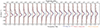 |
Fig. A.1. Two-component Gaussian fit (blue thick line) of CRISTAL-02 emission profile along each column in the position-velocity (p-v) diagram (grey lines) extracted along the kinematic major axis. The underlying p-v diagram from which the profiles are extracted is shown in Figure A.6 in the Appendix A. We assumed the narrow component (red) to trace the bulk rotation motion of the gas, which was then used for subsequent kinematics modelling, while the broad component (orange) is associated with the outflow and the interacting companion in the north (at offset |

CRISTAL-03: Best Disk, where the velocity gradient appears to align with the overall morphological PA of the HST and JWST images, but not with that of [C II], especially at the outer isophotes due to the protrusion at the south-west. Although this galaxy is the most poorly resolved in our sample, the NIRSpec/JWST data with 5× better angular resolution reveal a consistent rotational pattern in Hα (W. Ren et al., in prep.). This galaxy is also flagged as the most evident candidate for an AGN, which could potentially account for the protruded [C II] emission towards the south-west, and the slight deviation from the unidirectional SA locus in Fig. A.2.
CRISTAL-04a: Non-Disk, with a velocity gradient running from south to north and elevated dispersion along the zeroth velocity contour. However, the velocity isocontours deviate substantially from a spider diagram, and the p-v diagram along the major axis is primarily flat. The perturbation is most likely due to its recent minor-merger interaction with CRISTAL-04b (mass ratio ∼17:1, Herrera-Camus et al. 2025). CRISTAL-04a and CRISTAL-04b are identified as a ‘pair’ in Ikeda et al. (2025).
CRISTAL-04b: Non-Disk, where a blob of faint [C II] emission ∼ 10 kpc north of CRISTAL-04a that does not show a clear rotating signature. It could comprise two smaller substructures, as evidenced by the [C II] line map and the JWST images.
CRISTAL-06a: Non-Disk that is possibly a counter-rotating binary merger of two disks, where we observe a reversal in velocity gradient along the major axis, yet the individual components remain spatially unresolved at the current resolution. This system was also classified as a pair-merger in association with CRISTAL-06b in Le Fèvre et al. (2020) and is the only multiple-[C II] system in Ikeda et al. (2025). Alternatively, it could be a single disk with the approaching side at the east perturbed by CRISTAL-06b, as hinted by a velocity dispersion that peaks where the gradient is steepest. Ikeda et al. (2025) identified the multi-[C II] nature within CRISTAL-06a, while CRISTAL-06a and CRISTAL-06b are identified as a ‘pair’ in Ikeda et al. (2025).
CRISTAL-06b: Disk, located ∼ 10 kpc north-east of CRISTAL-06a with its velocity and dispersion fields consistent with a rotating disk. The slightly twisted velocity isocontours are likely a result of the perturbation from CRISTAL-06a, which is 8× more massive (Herrera-Camus et al. 2025).
CRISTAL-07a: Disk that exhibits a clear velocity gradient from north to south, but the northern part is perturbed by its interaction with CRISTAL-07b (mass ratio ∼2:1) in the early phase. In the kinematics modelling, we symmetrise the velocity dispersion profile from the receding and approaching sides (following Posses et al. 2025) to reduce the impact of the interaction on the intrinsic dispersion, as the receding side is much less perturbed.
CRISTAL-07b: Non-Disk, which is an interacting neighbour with CRISTAL-07a separated by ∼ 8 kpc; there is an overall velocity gradient stretching from east to west, but the isovelocity contours are more disrupted compared to CRISTAL-07a due to its lower mass. CRISTAL-07a and CRISTAL-07b are identified as a ‘pair’ in Ikeda et al. (2025), while CRISTAL-07 as a whole was classified as a pair-merger in Le Fèvre et al. (2020).
CRISTAL-07c: Non-Disk that is an interacting system of comparable masses located at 140 kpc west of CRISTAL-07a and CRISTAL-07b.
CRISTAL-08: Disk that exhibits a remarkably smooth velocity gradient, although there is a change of isovelocity contours PA from south to west (visible also in the SA locus), likely due to non-circular motion along the minor axis (R. Herrera-Camus et al., in prep.). The velocity dispersion peaks at the south-west corner, away from the morphological centre and peak of the [C II] line emission; The JWST colour image shows a very clumpy appearance (see also the F444W residual image in Fig. B.1) similar to the galaxy in Tanaka et al. (2024) at z = 4.91, with clumps of various colours distributed from 8 o’clock to 2 o’clock positions. The Disk classification is consistent with the ‘rotating disk’ classification in Le Fèvre et al. (2020). Herrera-Camus et al. (2025) will present the detailed properties of the clumps.
CRISTAL-09: Disk observed as a compact object in the HST image, JWST reveals extended stellar light in the south-west at faint levels. The extended stellar component is more apparent in the residual left after subtracting a Sérsic model (Fig. B.1). [C II] data provides tentative evidence of disk rotation but is still limited by the angular resolution and S/N. This system was classified as a pair-merger in Le Fèvre et al. (2020).
CRISTAL-10a: Non-Disk, for which no JWST image is available. Based on the HST data, Ikeda et al. (2025) classified it as a multi-UV system, with the two UV components separated by ∼5.5 kpc. [C II] line map shows a consistent separation of the two components. Consider the two components as one system, it exhibits a monotonic velocity gradient from north-east to south-west across the two components, with a prominent dispersion peak where the velocity gradient is steepest. However, the Gaussian fit errors at the dispersion peak are large due to low S/N. SA locus and p-v diagram reveal an abrupt velocity jump between the east (CRISTAL-10a-E) and west components, with a clear gap in the velocity structure, coinciding with that in the HST image. This suggests that the velocity gradient is plausibly driven by the orbital motion of the two components. Notably, this system shows a strong [C II]/FIR deficit (Herrera-Camus et al. 2025), with prominent dust continuum emission where [C II] emission is weakest, particularly around the southern parts of both components. While this could indicate that the CRISTAL-10a and CRISTAL-10b are substructures of a single larger system, the [C II] kinematics does not support the interpretation for now, so we classify the system as a Non-Disk.
CRISTAL-10a-E: Disk that makes up the eastern component of CRISTAL-10a. Despite being in a potentially interacting system, it shows a very promising disk-rotating signature in its own velocity and dispersion maps. The SA locus and p-v diagram resemble a disk-like system but also exhibit features indicative of interaction with the western component.
CRISTAL-11: Disk, for which we observed a velocity gradient from south-east to north-west, with a dispersion peak near the morphological centre. The kinematic PA is aligned with the morphological PA in both JWST and HST images with a difference of < 10°. However, the north-west region appears more dust-attenuated and has a distinct colour compared to the south-east, suggesting a possible merger of the two systems. Higher resolution data would be required to discern the true nature of this system. Nevertheless, based on the available data, we maintain our classification as a Disk. Le Fèvre et al. (2020) classified this system as ‘extended and dispersion-dominated’.
CRISTAL-12: Disk that is the least massive system among CRISTAL, with a shallow velocity gradient. It is classified as ‘compact’ in Le Fèvre et al. (2020) and, even with our higher resolution data, it remains poorly resolved, with only a tentative velocity gradient from west to east. There is a faint [C II] emission blob ∼4 kpc away in the north-west, but no visible counterpart in HST and JWST images. This emission is linked to the elevated dispersion in the north-west. This feature is also seen in other Disk systems, CRISTAL-02, 15, 19 (and 03, although poorly resolved), which may suggest an outflow origin of the gas. However, except for CRISTAL-02, deeper data will be required to confirm this speculation.
CRISTAL-13: Non-Disk that was already noted by Ikeda et al. (2025) about its multi-UV appearance in HST, JWST images further reveal the intriguing structure of the eastern and western components. The compact western source is dominated by an older stellar population (Lines et al. 2025) situated adjacent to a clumpy, blue eastern tail. The clump properties are addressed in Herrera-Camus et al. (2025). While both the velocity and dispersion maps exhibit characteristic signatures of a rotating disk, the p-v diagrams along both the major and minor axes show features that deviate substantially from typical disk-like rotation. SA indicates receding motion along the blue tail, suggesting that this system is likely the result of a merger between the western and eastern sources.
CRISTAL-14: Non-Disk, for which we observed an apparent velocity gradient from north-east to south-west. However, a centralised dispersion peak is absent. Furthermore, the p-v diagrams do not display the characteristic patterns associated with disk-like rotation. Both HST and JWST images reveal a western component with a distinct colour that is faint in [C II]. The [C II] emission predominantly traces the eastern component, which contributes the majority of the velocity gradient. Therefore, it is likely that this system is similar to CRISTAL-13, with the eastern source being in a close encounter with the western source.
CRISTAL-15: Best Disk, where we observe a velocity gradient from south-east to north-west, which agrees with the unidirectional locus traced by SA. An extended [C II] structure is present at the north-east of the kinematic minor axis, which could indicate slow outflowing gas (see also CRISTAL-12), as there is no significant broad emission component in the integrated spectrum. The ‘root’ of this extended structure is also co-spatial with the elevated dispersion in the dispersion map. JWST data reveal three clumps of bluer colour embedded within a redder disk, which is also more evident in the F444W residual image in Fig. B.1. We notice that the peak-to-peak velocity difference of CRISTAL-15 is only 50 km s−1, and our ALMA data cube is binned to 20 km s−1, which barely samples the velocity gradient. The data cube binned to 10 km s−1 is too low S/N for robust extraction of the RC and dispersion profile. As a result, the derived velocity dispersion in Sect. 5 for CRISTAL-15 may still be contaminated by the contribution of the unresolved velocity gradient.
CRISTAL-16a,b: Non-Disk that is similar to CRISTAL-01b and CRISTAL-06, this system is an interacting pair consisting of at least two companions, CRISTAL-16a and CRISTAL-16b, separated by a distance of ∼5.3 kpc. The eastern companion, CRISTAL-16a, appears to be composed of two clumps separated by ≲2 kpc, similar to CRISTAL-02, although it is unclear whether these clumps represent separate galaxies in a merger, or multiple star formation clumps within a galaxy. The [C II] line map reveals two barely resolved emission peaks co-spatial with the two companions of CRISTAL-16a. When considering CRISTAL-16a as a whole, the global velocity gradient is aligned with the morphological minor axis. Interestingly, the zeroth-velocity contour coincides with the dispersion peaks, suggesting a possible scenario in which two disk-like systems are approaching each other along their respective minor axes. The JWST/F444W image (Fig. B.1) reveals a conceivable connecting ‘bridge’ between the north-east and south-west clumps within CRISTAL-16a, providing further evidence for an interaction. CRISTAL-16b is too faint in [C II] for kinematics extraction. Overall, the CRISTAL-16a system bears similarities to CRISTAL-07a and 07b, but perhaps with a different orbital configuration. However, the individual components remain spatially unresolved at the current resolution.
CRISTAL-19: Best Disk, where the velocity map, SA locus and p-v diagram all show a coherent velocity gradient with little deviation from symmetry. The dispersion peak coincides with the position of the steepest velocity gradient. There is no evidence of a physically associated neighbour in the available data. Despite having a high intrinsic dispersion (σ0 = 65 km s−1), the system’s Vrot/σ0 ≈ 2.2 ratio indicates it is not dispersion-dominated, contrary to the classification in Le Fèvre et al. (2020).
CRISTAL-20: Best Disk that is one of the CRISTAL pilot galaxies first studied by Herrera-Camus et al. (2022), which also presented its outflow properties. The velocity map shows the typical rotating pattern of a disk, while the dispersion map shows the expected outflow signature at the north-west. SA aligns uni-directionally with the observed gradient in the velocity map; p-v diagrams along the major axis show a clean S-shape, while along the minor axis, no velocity gradient is seen, indicative of a classical disk. Parlanti et al. (2025) presented the NIRSpec/JWST data of the ionised gas outflow traced by [O III]λ5007 Å and a merger scenario based on the ionised gas.
CRISTAL-21: Non-Disk, where the velocity gradient is from north to south, but the dispersion map shows multiple peaks. The SA locus also displays a chaotic distribution within the central region, which could indicate unresolved line-of-sight mergers. It is consistent with the very elongated shape of the p-v diagram, stretching from −500 km s−1 to 500 km s−1 within the central ∼2 kpc region, indicative of an absence of a global velocity gradient. Although this could also be caused by a strong outflow at the centre, Lambert et al. (2023) found no evidence of outflows from the system, as indicated by the absence of a broad secondary component in the [C II] spectrum. Instead, the observed disturbed gas and dust emission, combined with its kinematic structure, suggest that the system is in a late-stage merger. NIRCam/JWST images reveal a blue ‘clump’ located at the east side of the [C II] light centre, which could be the merger companion.
CRISTAL-23a: Non-Disk that is one of the companions (source C) in the ‘triple-merger’ system was first studied in detail by Jones et al. (2021). As noted by Jones et al. (2021), it is in proximity to the massive protocluster PC1 J1001+0220 (Lemaux et al. 2018). Since it lies along the major axis of the protocluster and is only ∼ 3.5 Mpc from the north-east component of this protocluster, it could be associated with the system in a filamentary structure. Because of a different slit angle chosen, we observe a velocity gradient from north to south of this source, in contrary to Jones et al. (2021). The p-v diagram, however, exhibits substantial broadening along the velocity axis in the central region, which is inexplicable by a disk origin (e.g. an outflow).
CRISTAL-23b: Disk, labelled as ‘source E’ in Jones et al. (2020). The velocity gradient exhibits a clear east-west orientation, consistent with SA analysis. The velocity dispersion is elevated around the zero-velocity contour. The p-v diagram along the major axis displays a characteristic disk profile, whereas the minor axis p-v diagram shows a slight deviation, likely attributed to the ongoing interaction with CRISTAL-23a.
CRISTAL-23c: Disk that was also noted by Devereaux et al. (2024). It is the least luminous of the three sources in the CRISTAL-23 system and is likely to be rotating. It is separated from CRISTAL-23a and 23b in velocity by ∼ 300 km s−1 and spatially by 18 kpc. The velocity and dispersion map of this galaxy showed signs of disk rotation but is slightly perturbed by its interaction with CRISTAL-23a and 23b. It is the ‘source W’ in Jones et al. (2020).
CRISTAL-24: Non-Disk, with multiple dispersion peaks in the dispersion map; the SA does not show a large-scale velocity gradient, with a closely spaced locus suggesting a line-of-sight merger, which is further supported by the almost vertical position-velocity diagram along the major axis. Morphological and kinematic studies by Devereaux et al. (2024) rejected the outflow scenarios. This galaxy has the largest integrated line width, σint ≈ 300 km s−1. Although CRISTAL-07 is 130 kpc (projected) away, it is not associated with CRISTAL-24 with a redshift difference of Δz ≈ 0.6.
CRISTAL-25: Non-Disk, for which Devereaux et al. (2024) previously dismissed the merger scenario based on the HST morphology and dust continuum emission; however, the disjoint velocity structure in the p-v diagram, the well-defined velocity gradients of each component (Fig. A.7), with the northern component displaying a clear dispersion peak, could be indicative of a merger.
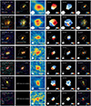 |
Fig. A.2. Gallery showing the multi-wavelength properties of the Best Disks. The first column displays the colour-composite images from HST, and if available, NIRCam/JWST images are shown in the second column. The third to fifth columns are ALMA images of [C II] emission, shown as line intensity, velocity, and velocity dispersion maps. The velocity and velocity dispersion maps are obtained by pixel-by-pixel single Gaussian fitting to the natural-weighted line cube, binned at ΔV = 20 km s−1 spectral resolution. They are not corrected for spectral broadening, beam-smearing and projection. The last column shows the spectro-astrometry (SA) measurement overlaid on HST (or NIRCam/JWST if available) colour images, in which the sizes and transparencies of the points are proportional to the positional uncertainties derived using Equation 1 in Condon et al. (1998). For all panels, the contours correspond to the intensities of the [C II] line map, plotted from 1.5σ to 3σ. |
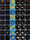 |
Fig. A.4. Same as Figure A.2, but for the Non-Disk. For CRISTAL-01a and 04b, we subtract the bright companions to improve visual contrast. |
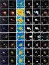 |
Fig. A.4. (Continued.) |
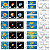 |
Fig. A.5. [C II] line maps, velocity maps, dispersion maps, position-velocity (p-v) diagrams (with median filtering applied for visual purposes), integrated spectra and shifted spectra of the Best Disk. In the [C II] line maps, the dashed pairs of arcs delineating the emission indicate the disk’s apparent morphological position angle (PAm, black) and the kinematic major axis (white). The solid pair of arcs represents the intrinsic PAm after correcting for the beam. In the p-v diagrams, the black and white horizontal bars correspond to 1″ and the synthesised beam FWHM, respectively. |
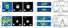 |
Fig. A.5. (Continued.) |
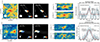 |
Fig. A.6. (Continued.) |
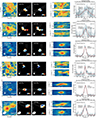 |
Fig. A.7. Same as Figure A.5, but for the Non-Disk. For CRISTAL-01a and CRISTAL-04b, the bright companions are subtracted from the line maps for better visual contrast. |
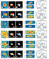 |
Fig. A.7. (Continued.) |
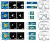 |
Fig. A.7. (Continued.) |
Appendix B: Structural parameters fit of NIRCam/F444W images
We fit the 2D light distributions of the galaxies observed with NIRCam/JWST F444W with imfit (Erwin 2015), accounting for the PSF. The PSF model adopted is described in Li et al. (2024). We assume a Sérsic profile with variable Sérsic index n and fixed n = 1. When let free, n freely varying within [0.5, 6]. We also let the effective radius (Re), the ellipticity e = 1 − b/a, and the position angle (PA) of the major axis as free parameters. Table B.1 lists the best-fit structural parameters of the galaxies for variable n. Average Sérsic index and effective radius are ⟨n⟩ = 1.1 ± 0.2, ⟨Re4.4μm⟩ = 1.46 ± 0.04 kpc, respectively. The effective radius is ∼ 1.5× that of the rest-frame UV emission ⟨ReUV⟩ ≈ 0.98 kpc (for the same sources considered, Ikeda et al. 2025). Our ⟨Re4.4μm⟩ is comparable to that of the dust continuum emission ⟨Redust⟩ ≈ 1.78 kpc (Mitsuhashi et al. 2024), but is smaller than the [C II] sizes ![Mathematical equation: $ \langle R_\mathrm{e_{[{\mathrm{C}{\small { {\text{ II}}}}}]}}\rangle $](/articles/aa/full_html/2025/09/aa55362-25/aa55362-25-eq183.gif) ≈ 1.9 kpc (Ikeda et al. 2025). Fixing n = 1 in our fit gives ⟨Re4.4μm⟩ = 1.77 kpc. For consistency, we used the result of n = 1 Re as the initial guess for the dynamical modelling.
≈ 1.9 kpc (Ikeda et al. 2025). Fixing n = 1 in our fit gives ⟨Re4.4μm⟩ = 1.77 kpc. For consistency, we used the result of n = 1 Re as the initial guess for the dynamical modelling.
For comparison, van der Wel et al. (2014), which covers 0 < z < 3 galaxies observed in the H160 band, the expected value for SFGs extrapolated to z = 5 and log M*/M⊙ = 10 is 2.4 kpc, our Re4.4μm is on average 40% smaller, but is still within the ∼0.2 dex scatter at z ≈ 3.
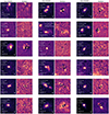 |
Fig. B.1. Examples of Sérsic fits and residuals of CRISTAL galaxies observed in JWST/F444W (rest-frame 0.7 μm at z ∼ 5). North is up for all images. For galaxies with multiple components, we simultaneously fit all components, each characterised by a single Sérsic profile. The resulting half-light radii (Re), Sérsic indices (n), and position angles (PA, measured counter-clockwise from the north) are listed in Table B.1 and annotated in the figures in order of increasing Re. Except in a few cases, such as CRISTAL-09, 12, and 14, the residuals exhibit clumpy structures and asymmetries in the light distributions due to multiple discrete clumps. |
Rest-frame optical to near-IR (F444W) structural parameters fitted by imfit.
Appendix C: Molecular gas fractions fmolgas
Previous studies of MS SFGs at z ∼ 1–3 have shown that their gas kinematics are closely tied to their molecular gas content (e.g. Wisnioski et al. 2015; Übler et al. 2019) inferred from scaling relations. We similarly explore the relationship between the kinematic properties of CRISTAL disks and their gas fractions in Sects. 6.1–6.2. As a first step, we need to estimate the gas content of our sample galaxies.
Measuring the gas content of CRISTAL galaxies using CO emission, which is a well-calibrated H2 tracer at low-z, is challenging in our case due to the cosmic dimming effect and typically low metallicities of galaxies, exacerbated by the higher temperature of the cosmic microwave background for lower–J transitions (TCMB(z) = 2.73(1 + z) K). Furthermore, the lack of multi-band observations for all galaxies, which would be necessary to constrain the full far-infrared (FIR) SED shape (e.g. Béthermin et al. 2015; Kaasinen et al. 2019), means that the only feasible estimator for most galaxies in CRISTAL5 is to infer gas masses from the single-band dust continuum emission measured in the Rayleigh-Jeans (R-J) tail of the FIR SED following the method of Scoville et al. (2016, 2017).
With the rest frequencies probed by the Band-7 (343.5 GHz) continuum data and if we adopt λ0 = 100 μm similar to Faisst et al. (2020b), which is the wavelength where optical depth reaches unity, and single dust temperature of Tdust = 50 K (see discussion below), then we can assume the R-J regime criterion is still satisfied and the optically-thin approximation is valid. We measure the dust continuum fluxes on the image directly using the curve-of-growth method. They are in general good agreement with Mitsuhashi et al. (2024).
We infer the gas mass Mgas from the observed flux density Sνobs of the Band-7 dust continuum (λobs ≈ 850–1050μm) in the R-J regime following Eq. (3) in Tacconi et al. (2020):
 (C.1)
(C.1)
We introduced the R-J departure coefficient ΓR − J back to Eq. (C.1) to account for the deviation of dust temperature from 25 K, which was originally used in Tacconi et al. (2020). ΓR − J is defined as (Eq. (6) in Scoville et al. 2016)
 (C.2)
(C.2)
The Γ0 factor in Eq. (C.1) is taken at z = 0, Td = 50 K (see below) and at the respective νobs for different observations. On average, the coefficient  .
.
We adopt a dust temperature6Td = 50K, based on Villanueva et al. (2024) FIR SED modelling of CRISTAL-22, which benefits from the continuum data observed at multiple bands (but see also Béthermin et al. 2020; Faisst et al. 2020b and Sommovigo et al. 2022). We assume a dust emissivity index7 of β = 1.8, the suggested value by Scoville et al. (2016) based on the findings of the Planck Collaboration XXI (2011). Such a choice is close to the value of β = 2 measured by Villanueva et al. (2024). We adopt the R-J luminosity-to-mass ratio αdust,0 = 6.7 × 10¹⁹ erg (s Hz M⊙)−1. Assuming αdust, 0 = 8 × 10¹⁹ erg (s Hz M⊙)−1 following Tacconi et al. (2020)8 would result in lower Mgas by ≲0.1 dex in median.
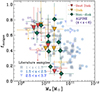 |
Fig. C.1. Molecular gas fraction, fmolgas, (Equation C.3) as a function of stellar mass as inferred from the Band-7 dust continuum based on Equation C.1. The points are colour-coded by their classifications described in Section 3. The empty circles represent upper limits. The median gas fraction of the CRISTAL sample is ∼ 0.5. Our measurements are in broad agreement with those reported by Dessauges-Zavadsky et al. (2020) for the ALPINE samples (purple hexagons), in which we both observe a similar slope of dependence of fmolgas on M⋆, similar to that of the lower redshifts 1≲ z ≲6 star-forming galaxies compiled by Dessauges-Zavadsky et al. (2020) and references therein (light grey to blue markers). |
The gas-to-dust ratio, δgd ≔  , anti-correlates with metallicity (Eq. (10) in Genzel et al. (2015), see also Leroy et al. (2011) and Tacconi et al. (2018)). We estimate metallicity using the mass-metallicity relation (MZR) inferred from NIRSpec/JWST data of galaxies at z = 4–10 by Nakajima et al. (2023), which applies to galaxies with masses in the range 107.5 < M⋆ < 109.5. We extrapolate the MZR to cover the more massive galaxies in our sample. Our sample’s average metallicity ⟨12 + log(O/H)⟩ = 8.27 ± 0.05, and the corresponding gas-to-dust ratio coefficient is
  . The uncertainties represent the scatter in the Nakajima et al. (2023)’s relation, which would translate to no more than 0.05 dex difference to the final Mgas.
We note that individual gas-phase metallicities (except for CRISTAL-08, 21, and 23) can be determined from rest-frame optical strong line ratios using NIRSpec/JWST data (R = 1000), and the values are consistent with our adopted metallicities. A more detailed discussion of these results will be presented in A. Faisst (in prep.) and S. Fujimoto et al. (in prep.). Parlanti et al. (2025) presented the metallicity measurement of CRISTAL-20 (HZ4) which is 12 + log(O/H) ∼ 8.3.
Based on the Mgas derived above, Fig. C.1 and Table 3 show the gas fraction of the CRISTAL sample. We define the gas fraction as
 (C.3)
(C.3)
The median gas fraction fmolgas = 0.51. This is also consistent with the expected value from Tacconi et al. 2020’s relation at z = 5 for M* = 1010 M⊙, which is ∼ 0.53. For CRISTAL-22, our measured fmolgas
 is consistent with that inferred by Pavesi et al. (2019) from VLA CO(2-1) data. For CRISTAL-01a, 08, 12, 14, 15, 16, 23b, 23c, the measured fmolgas are upper-limits because the dust continuum fluxes are below the S/N threshold defined in Mitsuhashi et al. (2024). There is insufficient co-spatial dust emission for CRISTAL-04b and 07b, so we have no fmolgas measurement for those. The stellar mass M⋆ are based on SED fitting results presented in Li et al. (2024) for those sources with NIRCam/JWST images; if not, then we adopt the values from Mitsuhashi et al. (2024).
Our fmolgas measurements, regardless of their kinematics types, are in good agreement with Dessauges-Zavadsky et al. (2020) (purple hexagons in Fig. C.1), which measured fmolgas for the ALPINE sample based on (i) [C II] emission following Zanella et al. (2018) (ii) rest-frame 850 μm extrapolated from the FIR SED template of Béthermin et al. (2017) and (iii) dynamical mass assuming virialised spherical systems. We also recover a steep relation between fmolgas and the stellar mass of the systems, similar to the lower-redshift studies following the same selection in Dessauges-Zavadsky et al. (2020) and references therein.
Inferring Mgas with the method described above is subject to several important caveats. Firstly, the assumption that the Band-7 continuum lies on the R-J tail is sensitive to the adopted single dust temperature, Td = 50 K. If Td is lower, the R-J assumption breaks down, particularly for the highest-redshift sources in our sample. Using Td = 25 K would increase Mgas by ∼ 0.5 dex. Furthermore, we lack information on the mass-weighted Td. The absence of longer wavelength data implies that we are neglecting a dominant colder component of the dust. Additionally, the adopted values for αdust, 0 and δgd are based on lower-redshift measurements and calibrations, although Mgas appears to be relatively insensitive to these values within the possible range.
An alternative method for estimating Mgas is by using the [C II] luminosity. If we apply the relation from Zanella et al. (2018) (their Eq. (2)), we find that the resulting Mgas is systematically higher by 0.23 dex (in terms of the median), but still within the 0.3 dex scatter of the relation. We also observe a significant correlation between the dust- and [C II]-inferred Mgas values (with Kendall’s  , p ≪ 0.05).
Overall, varying our assumptions and using different methods will very likely lead to higher Mgas and fmolgas values, which, as a corollary, a lower Toomre Q values, as inferred from Eq. (3) in Sect. 6.3. This would not change the main findings, namely, that CRISTAL disks are gravitationally (un)stable and the correlations discussed in Sect. 6.2. However, the statistical significance of the correlations would be weaker given the more uncertain Mgas and fmolgas.
Appendix D: Literature sample of Vrot and σ
Compilation of literature references for rotational velocity and velocity dispersion from local to z ≲ 8 galaxies.
Table D.1 lists the literature samples discussed in Sect. 6.1 and shown in Fig. 9.
Literature sample with multi-phase gas kinematics measurement.
Appendix E: Model velocity profiles
Fig. E.1 shows the intrinsic σ0, circular velocity profiles of the DM and the baryonic components. The DM fraction profile inferred from the circular velocities fDM(< R) = Vcirc, DM2(R)/Vcirc, tot2(R) is shown as the secondary y-axis.
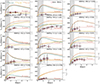 |
Fig. E.1. Intrinsic baryonic Vcirc, bary, DM, Vcirc, DM, and total circular velocity Vcirc, tot profiles of the CRISTAL disk sample with asymmetric drift correction. The grey circles mark the folded 1D observed velocity profiles, and the red squares show the observed profiles extracted from the DysmalPy-modelled cubes. The red dashed line indicates the intrinsic constant velocity dispersion σ0, intrinsic. The DM fraction fDM(< R) = Vcirc, DM2(R)/Vcirc, tot2(R) is shown in solid grey curves. The grey dashed vertical line marks the disk’s effective radius. |
Appendix F: Comparison to K18 model with total SFR
In Sect. 6.4, we compare the σ0–ΣSFR with the Krumholz et al. (2018) analytic models. Here, we also compare the CRISTAL values with the models in σ0–SFR space. Integrating Eq. (4) with radius, the total SFR is related to σg by (Eq. (60) in Krumholz et al. (2018)):
![Mathematical equation: $$ \begin{aligned} \begin{split} \text{ SFR} =&\sqrt{\frac{2}{1+\beta }}\frac{\phi _{a}f_{\rm SF}}{\pi GQ}f_{\rm g,Q}v_{\phi ,\mathrm{out}}^2\sigma _g \\&\cdot \text{ max}\left[\sqrt{\frac{2(1+\beta )}{2f_{g,P}\phi _{\rm mp}}}\frac{8\epsilon _{\rm ff} f_{g,Q}}{Q},\frac{t_{\rm orb,out}}{t_{\rm sf, max}}\right], \end{split} \end{aligned} $$](/articles/aa/full_html/2025/09/aa55362-25/aa55362-25-eq192.gif) (F.1)
(F.1)
while for ‘feedback-only’ (fixed Q) model (Eq. (62) in Krumholz et al. 2018):
 (F.2)
(F.2)
The definitions of the symbols and values adopted are described in Sect. 6.2 and Table F.1. Here the rotation velocity vϕ that is related to the radial gradient of the potential ψ, is set to be vϕ =  ∈ [100, 350] km s−1, in increments of 50 km s−1.
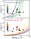 |
Fig. F.1. Same as Figure 11 but for σ0 vs total star formation rate (SFR). The solid lines are analytical models from Krumholz et al. (2018) based on Equations F.1 and F.2. |
All Tables
Compilation of literature references for rotational velocity and velocity dispersion from local to z ≲ 8 galaxies.
All Figures
|
Fig. 1. Parameter space of the CRISTAL sample in terms of surface densities of star formation rate (ΣSFR, left) and baryons (Σbar, right). For comparison, the z ∼ 2 MS galaxies observed in Hα (blue circles) and CO (red hexagons) by Nestor Shachar et al. (2023) are also shown. The inset of the left and right panels show the SFR-M⋆ and [C II]-sizes-M⋆ distributions of CRISTAL (green contour) and other studies at z ≳ 4 (yellow diamonds) (Neeleman et al. 2020; Rizzo et al. 2020, 2021; Fraternali et al. 2021; Herrera-Camus et al. 2022; Parlanti et al. 2023; Roman-Oliveira et al. 2023), respectively. The solid line in the left inset is the MS relation from Speagle et al. (2014) at z = 5, with the shading representing ±0.5 dex offset from the relation. For the purposes of illustration, the values of CRISTAL shown on the plots are adopted from ALPINE (Béthermin et al. 2020; Faisst et al. 2020a; Le Fèvre et al. 2020). CRISTAL provides a higher-resolution sample of MS SFGs that fills up the parameter space currently poorly explored by existing z ≳ 4 samples observed with [C II], which predominantly comprises starburst and compact galaxies. |
| In the text | |
|
Fig. 2. Ratios of observed half velocity gradient Vobs/2 and integrated line width (σint) of [C II] as a function of stellar mass M*. The black horizontal dashed line represents the distinction value (Vobs/2σint = 0.4), which demarcates the boundary between rotation- and dispersion-dominated systems, as commonly used in the literature. |
| In the text | |
|
Fig. 3. Velocity (top) and velocity dispersion (bottom) fields of CRISTAL galaxies placed on the ΔMS offset relative to the Speagle et al. (2014) MS relation. The velocity and dispersion fields correspond to those derived from the [C II] emission described in Sect. 3.3. For the velocity fields, the colour coding represents the relative velocity of the line emission with respect to the systemic velocity. For the dispersion fields, the colour coding indicates the widths (in standard deviation) of the 1D Gaussian fitted to the spectra of individual spaxels. All sources are shown in the same field of view of 3″ (∼20 kpc at z ∼ 5). The median beam size (0 |
| In the text | |
|
Fig. 4. Asymmetry measure of the velocity and velocity dispersion fields for the CRISTAL galaxies from Kinemetry (Krajnović et al. 2006) is shown in Fig. 4. The black dashed line represents the demarcation in Shapiro et al. (2008) at Kasym = 0.5. With this metric alone, we classify a system as disk-like if it falls below the dashed line and as a merger if it falls above. Over half of the samples fall below the dashed line. The pink (Kasym = 0.9) and green (Kasym = 0.3) lines indicate the modified demarcations. |
| In the text | |
|
Fig. 5. Comparison of the CRISTAL total disk fraction (yellow hexagon with red outline) to the mass-selected sample from Ferreira et al. (2023) based on CRISTAL mass range. The grey curve with square markers shows the ‘redshift-corrected’ trend of their high-mass bin. To more fairly compare with our sample, we further selected so that their star formation rates are within 1 dex from the Speagle et al. (2014) MS relation. The grey horizontal line indicates the redshift range of CRISTAL (4.4 < z < 5.7). The black solid curve with square markers represents the redshift evolution of disk fraction as reported by Ferreira et al. (2023) before their application of ‘redshift corrections’, which primarily account for surface-brightness effects in higher redshift objects. It would be a more equal comparison since we do not apply any such correction to the CRISTAL disk fraction. The inset shows the distribution of Best Disk, Disk, and Non-disk among the CRISTAL sample. |
| In the text | |
|
Fig. 6. Observed rotation curves (RCs) of the CRISTAL disk sample. The RCs are the fitted line velocity centroids of the position-velocity diagram extracted along the kinematic major axis. The RCs are grouped according to their kinematics types. The black curves are the extracted 1D model (in the same way as data) from the best-fit 3D model cube from DysmalPy. The 3D model cubes are projected and convolved with the beam, which gives rise to the apparent central peak in the velocity dispersion profile and the shallower velocity profiles. The two symmetric grey vertical lines about the dynamical centre indicate the effective radius. The synthesised beam size is shown as the horizontal black line at the top. CRISTAL-05 and 22a belong to Disk, their velocity profiles are shown in Posses et al. (2025) and Telikova et al. (2025), respectively. |
| In the text | |
|
Fig. 7. Intrinsic total circular velocity profiles Vcirc(R/Re, disk) of all CRISTAL disks, corrected for beam-smearing and projection effects. Colours in ascending order represent the CRISTAL ID (first column in Table 3). The individual Vcirc(R) of baryons and DM are presented in Figure E.1 in Appendix E. Thin, lighter coloured lines indicate the radial range beyond which the data are not covered. |
| In the text | |
|
Fig. 8. Intrinsic velocity dispersion, σ0, as a function of the number of resolution elements within the outermost measurable radius, Rout, and inclination (i). The Spearman and Kendall rank correlation coefficients (ρ and τ, respectively) do not indicate a significant correlation of σ0 with the inclination and resolution effects, although the uncertainties in both the coefficients and p-value are large. CRISTAL-03, which has Rout/beamHWHM = 1.6 is excluded in the correlation analysis in Sect. 6.2. |
| In the text | |
|
Fig. 9. Dynamical evolution of high-z galaxies. Top: Intrinsic velocity dispersion σ0 as a function of redshift for our disk sample (black hexagons with green outline) compared with the literature values (see Appendix D Table D.1). Bottom: Same but for the ratio between rotational velocity and σ0, Vrot/σ0. The solid and dashed black lines are the Übler et al. (2019)’s best-fit relations for galaxies at z < 4, for ionised and cold molecular gas, respectively. Where available, the points are colour-coded by their MS offset, ΔMS, relative to the Speagle et al. (2014) relation, otherwise in grey. The insets show the literature sample (see Table D.2) of the same galaxy with two gas tracers tracing different phases. The insets include the galaxies with large uncertainties, which are omitted in the main plots. The grey shading encloses the corresponding range in σ0 and Vrot/σ0 for Q ∈ [0.6, 2.0]. The definition of the Toomre Q parameter is presented in Sect. 6.3. |
| In the text | |
|
Fig. 10. Intrinsic velocity dispersion (σ0) and the ratio of rotation velocity at the effective radius (Vrot(Re)) to intrinsic velocity dispersion (σ0) as a function of five galaxy properties: molecular gas fraction (fmolgas), stellar mass (log(M⋆/M⊙)), offset from the main sequence (ΔMS), star formation rate surface density (ΣSFR), and molecular gas mass (log(Mgas/M⊙)). The dashed and solid grey curves in the first column are the predicted trends based on Equation (3) with Q fixed at Qcrit = 0.67, with a = 1 and a= |
| In the text | |
|
Fig. 11. σ0 vs ΣSFR of CRISTAL disks compared with analytical models from Krumholz et al. (2018). The solid lines in the upper panel show the σ0 values predicted from the Transport+Feedback model with orbital period torb = [30, 120] Myr. Similarly, for the lower panel, but for the ‘Feedback-only’ model. The results are broadly consistent with the ‘feedback+transport’ model, suggesting that the elevated velocity dispersion of normal star-forming galaxies at this epoch requires additional gravitational energy from mass transport across the disk. |
| In the text | |
|
Fig. 12. DM fraction, fDM, as a function of the circular velocity at the effective radius, Vcirc(Re) (left), and baryonic surface density, Σbary (right). The yellow and blue curves show the TNG100 (without adiabatic contraction) relations at z = 0 and z = 2 (Lovell et al. 2018), respectively. The pale blue and red shadings are measurements from RC100 at z < 1.2 and z < 2.5, respectively (Nestor Shachar et al. 2023). The thick grey dashed curve is the best-fit relation of z ∼ 2 star-forming galaxies from Wuyts et al. (2016). The CRISTAL sample statistics suggest a tentative anti-correlation with fDM(Re) and Σbary, although individual galaxy uncertainties are limited by the data depth. The horizontal dashed line denotes fDM for a maximal disk fDM ≔ 28% (van Albada et al. 1985). In the right panel, the two symbols plotted with only limit arrows represent CRISTAL-10a-E (upper limit) and CRISTAL-06b (lower limit). The stellar mass is only for CRISTAL-10a as a whole, which includes CRISTAL-10a-E, while no gas mass is available for CRISTAL-06b. |
| In the text | |
|
Fig. 13. DM fraction at effective radius (fDM(Re)) as a function of redshift. The fDM(Re) of individual CRISTAL disks (4 < z < 6) are represented by small diamonds, colour-coded by their Vcirc(Re). For comparison, we include lower redshift studies around z = 2 from Wuyts et al. (2016) (grey box-and-whisker) and the best-fit relation to the RC100 data set (Nestor Shachar et al. 2023) (black solid line for the redshift range covered and dashed line for the extrapolated range). For both observational studies, we consider only SFGs on the MS and the baryonic mass Mbary matched within 0.3 dex of the CRISTAL disks. The new best-fit relation to RC100, using the Mbary-matched sample, is shown in the legend. The trends predicted from the TNG100 simulation for M* = 1010 M⊙ and M* = 1011 M⊙ are shown in yellow and blue, respectively (Lovell et al. 2018). Overall, the CRISTAL disks tend to be baryon-dominated on galactic scales, with a median DM fraction of ∼18% (large green diamond) that is tentatively consistent with the extrapolated relation based on RC100. However, there is a significant scatter in the values among the sample, partly driven by the scattered distributions of circular velocity Vcirc(Re) (and Σbary) shown in Figure 12. |
| In the text | |
|
Fig. A.1. Two-component Gaussian fit (blue thick line) of CRISTAL-02 emission profile along each column in the position-velocity (p-v) diagram (grey lines) extracted along the kinematic major axis. The underlying p-v diagram from which the profiles are extracted is shown in Figure A.6 in the Appendix A. We assumed the narrow component (red) to trace the bulk rotation motion of the gas, which was then used for subsequent kinematics modelling, while the broad component (orange) is associated with the outflow and the interacting companion in the north (at offset |
| In the text | |
|
Fig. A.2. Gallery showing the multi-wavelength properties of the Best Disks. The first column displays the colour-composite images from HST, and if available, NIRCam/JWST images are shown in the second column. The third to fifth columns are ALMA images of [C II] emission, shown as line intensity, velocity, and velocity dispersion maps. The velocity and velocity dispersion maps are obtained by pixel-by-pixel single Gaussian fitting to the natural-weighted line cube, binned at ΔV = 20 km s−1 spectral resolution. They are not corrected for spectral broadening, beam-smearing and projection. The last column shows the spectro-astrometry (SA) measurement overlaid on HST (or NIRCam/JWST if available) colour images, in which the sizes and transparencies of the points are proportional to the positional uncertainties derived using Equation 1 in Condon et al. (1998). For all panels, the contours correspond to the intensities of the [C II] line map, plotted from 1.5σ to 3σ. |
| In the text | |
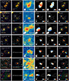 |
Fig. A.3. Same as Figure A.2, but for the Disk. |
| In the text | |
|
Fig. A.4. Same as Figure A.2, but for the Non-Disk. For CRISTAL-01a and 04b, we subtract the bright companions to improve visual contrast. |
| In the text | |
|
Fig. A.4. (Continued.) |
| In the text | |
|
Fig. A.5. [C II] line maps, velocity maps, dispersion maps, position-velocity (p-v) diagrams (with median filtering applied for visual purposes), integrated spectra and shifted spectra of the Best Disk. In the [C II] line maps, the dashed pairs of arcs delineating the emission indicate the disk’s apparent morphological position angle (PAm, black) and the kinematic major axis (white). The solid pair of arcs represents the intrinsic PAm after correcting for the beam. In the p-v diagrams, the black and white horizontal bars correspond to 1″ and the synthesised beam FWHM, respectively. |
| In the text | |
|
Fig. A.5. (Continued.) |
| In the text | |
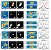 |
Fig. A.6. Same as Figure A.5, but for the Disk. |
| In the text | |
|
Fig. A.6. (Continued.) |
| In the text | |
|
Fig. A.7. Same as Figure A.5, but for the Non-Disk. For CRISTAL-01a and CRISTAL-04b, the bright companions are subtracted from the line maps for better visual contrast. |
| In the text | |
|
Fig. A.7. (Continued.) |
| In the text | |
|
Fig. A.7. (Continued.) |
| In the text | |
|
Fig. B.1. Examples of Sérsic fits and residuals of CRISTAL galaxies observed in JWST/F444W (rest-frame 0.7 μm at z ∼ 5). North is up for all images. For galaxies with multiple components, we simultaneously fit all components, each characterised by a single Sérsic profile. The resulting half-light radii (Re), Sérsic indices (n), and position angles (PA, measured counter-clockwise from the north) are listed in Table B.1 and annotated in the figures in order of increasing Re. Except in a few cases, such as CRISTAL-09, 12, and 14, the residuals exhibit clumpy structures and asymmetries in the light distributions due to multiple discrete clumps. |
| In the text | |
|
Fig. C.1. Molecular gas fraction, fmolgas, (Equation C.3) as a function of stellar mass as inferred from the Band-7 dust continuum based on Equation C.1. The points are colour-coded by their classifications described in Section 3. The empty circles represent upper limits. The median gas fraction of the CRISTAL sample is ∼ 0.5. Our measurements are in broad agreement with those reported by Dessauges-Zavadsky et al. (2020) for the ALPINE samples (purple hexagons), in which we both observe a similar slope of dependence of fmolgas on M⋆, similar to that of the lower redshifts 1≲ z ≲6 star-forming galaxies compiled by Dessauges-Zavadsky et al. (2020) and references therein (light grey to blue markers). |
| In the text | |
|
Fig. E.1. Intrinsic baryonic Vcirc, bary, DM, Vcirc, DM, and total circular velocity Vcirc, tot profiles of the CRISTAL disk sample with asymmetric drift correction. The grey circles mark the folded 1D observed velocity profiles, and the red squares show the observed profiles extracted from the DysmalPy-modelled cubes. The red dashed line indicates the intrinsic constant velocity dispersion σ0, intrinsic. The DM fraction fDM(< R) = Vcirc, DM2(R)/Vcirc, tot2(R) is shown in solid grey curves. The grey dashed vertical line marks the disk’s effective radius. |
| In the text | |
|
Fig. F.1. Same as Figure 11 but for σ0 vs total star formation rate (SFR). The solid lines are analytical models from Krumholz et al. (2018) based on Equations F.1 and F.2. |
| In the text | |
Current usage metrics show cumulative count of Article Views (full-text article views including HTML views, PDF and ePub downloads, according to the available data) and Abstracts Views on Vision4Press platform.
Data correspond to usage on the plateform after 2015. The current usage metrics is available 48-96 hours after online publication and is updated daily on week days.
Initial download of the metrics may take a while.