| Issue |
A&A
Volume 702, October 2025
|
|
|---|---|---|
| Article Number | A133 | |
| Number of page(s) | 30 | |
| Section | Interstellar and circumstellar matter | |
| DOI | https://doi.org/10.1051/0004-6361/202553830 | |
| Published online | 14 October 2025 | |
ALMA-IMF
XIX. C18O (J = 2–1): Measurements of turbulence in 15 massive protoclusters
1
Departamento de Astronomía, Universidad de Concepción,
Casilla 160-C,
Concepción,
Chile
2
Franco-Chilean Laboratory for Astronomy, IRL 3386, CNRS and Universidad de Chile,
Santiago,
Chile
3
Univ. Grenoble Alpes, CNRS, IPAG,
38000
Grenoble,
France
4
Department of Astronomy, University of Florida,
PO Box
112055,
USA
5
Instituto de Radioastronomía y Astrofísica, Universidad Nacional Autónoma de México, Morelia,
Michoacán
58089,
Mexico
6
National Astronomical Observatory of Japan, National Institutes of Natural Sciences,
2-21-1 Osawa, Mitaka,
Tokyo
181-8588,
Japan
7
Department of Astronomical Science, SOKENDAI (The Graduate University for Advanced Studies),
2-21-1 Osawa, Mitaka,
Tokyo
181-8588,
Japan
8
S. N. Bose National center for Basic Sciences,
Sector-III, Salt Lake,
Kolkata
700106,
India
9
Departament de Física Quàntica i Astrofísica (FQA), Universitat de Barcelona (UB),
Martí i Franquès 1,
08028
Barcelona, Catalonia,
Spain
10
Institut de Ciències del Cosmos (ICCUB), Universitat de Barcelona,
Martí i Franquès 1,
08028
Barcelona, Catalonia,
Spain
11
Institut d’Estudis Espacials de Catalunya (IEEC),
Esteve Terradas 1, Edifici RDIT, Ofic. 212 Parc Mediterrani de la Tecnologia (PMT) Campus del Baix LLobregat -– UPC
08860
Castelldefels (Barcelona), Catalonia,
Spain
12
Laboratoire d’Astrophysique de Bordeaux, Univ. Bordeaux, CNRS,
UMR 5804,
33615
Pessac,
France
13
School of Physics and Astronomy, Yunnan University,
Kunming,
650091,
PR
China
14
Laboratoire d’Astrophysique de Bordeaux, Univ. Bordeaux, CNRS,
B18N, allée Geoffroy Saint-Hilaire,
33615
Pessac,
France
15
Laboratoire de Physique de l’École Normale Supérieure, ENS, Université PSL, CNRS, Sorbonne Université, Université Paris Cité,
75005
Paris,
France
16
Observatoire de Paris, PSL University, Sorbonne Université, LERMA,
75014
Paris,
France
17
Instituto Argentino de Radioastronomía (CCT-La Plata, CONICET; UNLP; CICPBA),
C.C. No. 5,
1894,
Villa Elisa, Buenos Aires,
Argentina
18
SKA Observatory, Jodrell Bank, Lower Withington,
Macclesfield
SK11 9FT,
UK
19
Astronomy Department, Universidad de Chile,
Casilla 36-D,
Santiago,
Chile
20
Departments of Astronomy and Chemistry, University of Virginia,
Charlottesville,
VA
22904,
USA
★ Corresponding author: This email address is being protected from spambots. You need JavaScript enabled to view it.
Received:
20
January
2025
Accepted:
8
August
2025
Abstract
ALMA-IMF is a Large Program of the Atacama Large Millimeter/submillimeter Array (ALMA) that aims to determine the origin of the core mass function (CMF) of 15 massive Galactic protoclusters (~1.0–25.0 × 10³ M⊙ within ~2.5 × 2.5 pc2) located toward the Galactic plane. In addition, the objective of the program is to obtain a thorough understanding of their physical and kinematic properties. Here we study the turbulence in these protoclusters with the C18O (2–1) emission line using the sonic Mach number analysis (Ms) and the size-linewidth relation. The probability distribution functions (PDFs) for Ms show a similar pattern, exhibiting no clear trend associated with evolutionary stage, peaking in the range between 4 and 7, and then extending to ~25. Such values of Ms indicate that the turbulence in the density regime traced by the C18O line inside the protoclusters is supersonic in nature. In addition, we compared the non-thermal velocity dispersions (σnth,C18O) obtained from the C18O (2–1) line with the non-thermal line widths (σnth, DCN) of the cores obtained from the DCN (3–2) line. We observed that, on average, the non-thermal linewidth in cores is half that of the gas surrounding them. This suggests that turbulence diminishes at smaller scales or dissipates at the periphery of the cores. Furthermore, we examined the size-linewidth relation for the structures we extracted from the position-position-velocity C18O (2–1) line emission cube with the dendrogram algorithm. The power-law index (p) obtained from the size-linewidth relation is between 0.41 and 0.64, steeper than the Kolmogorov law of turbulence, as expected for compressible media. In conclusion, this work is one of the first to carry out a statistical study of turbulence for embedded massive protoclusters.
Key words: ISM: clouds / ISM: kinematics and dynamics / ISM: molecules
© The Authors 2025
 Open Access article, published by EDP Sciences, under the terms of the Creative Commons Attribution License (https://creativecommons.org/licenses/by/4.0), which permits unrestricted use, distribution, and reproduction in any medium, provided the original work is properly cited.
This article is published in open access under the Subscribe to Open model. This email address is being protected from spambots. You need JavaScript enabled to view it. to support open access publication.
1 Introduction
Turbulence plays a crucial role in shaping the interstellar medium (ISM), which is essential for understanding the evolution of molecular clouds (Solomon et al. 1987; Heyer & Brunt 2004; Koley 2019; Petkova et al. 2023; Koley 2023b; Green et al. 2024). The interplay between turbulence, magnetic fields, and gravity leads to the fragmentation of dense clumps, resulting in the formation of cores and eventually in the formation of new stars (Busquet et al. 2016; Wang et al. 2020; Stutz & Gould 2016; Stutz 2018; Palau et al. 2021; Koley et al. 2021, 2022; Rawat et al. 2024; Sanhueza et al. 2025; Reyes-Reyes et al. 2024). Various studies have indicated that in molecular clouds, turbulence is supersonic in nature. On a large scale, supersonic turbulence can prevent global collapse and supports the structure of molecular clouds (Mac Low & Klessen 2004; Federrath 2015). On a small scale, turbulence also affects the fragmentation of dense cores, and stars begin to form when turbulence dissipates (Myers 1983; Goodman et al. 1998; Nakano 1998; Koley 2023a). In the interstellar medium, turbulence plays a key role in determining the star formation rate (SFR; Federrath & Klessen 2012; Federrath 2015; Orkisz et al. 2017; Federrath 2018). It is thus important to examine the nature of turbulence for a better understanding of the star formation process.
In molecular clouds, turbulence is measured by a variety of methods. These include analysis of the sonic Mach number (Ms), examination of the size-linewidth relationship, principal component analysis (PCA), and power spectrum analysis (Heyer & Brunt 2004; Orkisz et al. 2017; Petkova et al. 2023). For example, using the examination of Ms, it has been shown in multiple studies that in molecular clouds, turbulence is supersonic in nature (Orkisz et al. 2017; Wang & Wang 2023). In addition, using the size-linewidth relation, previous studies have shown that in molecular clouds the power-law index (p) is close to 0.50. For example, Solomon et al. (1987) examined the size-linewidth relation for 273 molecular clouds using the CO molecular line and noted that p is 0.50. Similarly, using PCA, Heyer & Brunt (2004) demonstrated that the velocity structure function varies as a function of spatial scale with a value of p of 0.49. In addition to these observational studies, several numerical studies have also shown that the power-law index of velocity dispersion in the molecular cloud is steeper than the standard Kolmogorov law of turbulence (p = 0.33) and close to 0.50 (Kolmogorov 1941; Fleck 1983; Kowal & Lazarian 2007).
The ALMA-IMF is an Atacama Large Millimeter/ submillimeter Array (ALMA) Large Program designed to observe 15 massive protoclusters in our Galaxy. Here, the distance of the 15 protoclusters ranges between 2.0 kpc and 5.5 kpc, with a mean value of ~3.9 kpc. This suitable distance range allows us to trace the area of more than 1 pc2 toward the highest column density area obtained from the ATLASGAL survey (Csengeri et al. 2017). In addition, the unprecedented resolution of ALMA allows us to achieve and investigate ~0.01 pc core-scale structures in these regions. The gas masses of the ALMA-IMF protocluster sample are ~1.0–25.0 × 10³ M⊙. The majority of the protoclusters are located within ± 0.5° of the Galactic plane, where most of the massive gas clouds reside. Motte et al. (2022) and Galván-Madrid et al. (2024) classified the evolutionary stage of these 15 protoclusters based on the flux ratio between the 1.3 and 3.0 mm continuums and the H41α emission. In their study, the authors found that during the evolution of the protoclusters, the flux ratio between 1.3 mm and 3.0 mm continuums decreases, and H41α emission increases at the same time. Based on these constraints, they classified six protoclusters as young, five protoclusters as intermediate, and the remaining four protoclusters as evolved. We provide a general overview of the 15 protoclusters in Table 1.
This Large Program utilizes data from ALMA 12 m and 7 m arrays as well as the total power (TP) in two bands: Band 3 (3.0 mm) and Band 6 (1.3 mm) (Motte et al. 2022; Ginsburg et al. 2022; Cunningham et al. 2023). The observations include several spectral lines and continuum in two bands. Two continuum images at 1.3 and 3.0 mm mainly tracing thermal dust emission are used to investigate the key properties of the cores (which are on the verge of star formation), such as their luminosity, temperature, and mass (Motte et al. 2018; Pouteau et al. 2022; Armante et al. 2024; Louvet et al. 2024). Likewise, the spectral energy distribution (SED) of thermal dust emission is also used to determine the dust temperature within the protoclusters (Brouillet et al. 2022; Bonfand et al. 2024; Dell’Ova et al. 2024; Motte et al. 2025). Furthermore, the DCN (3–2) spectral line provides insight into core kinematics (Cunningham et al. 2023). Another prominent spectral line, N2H+(1–0), allows us to study the kinematics of the dense cold gas inside the protoclusters (Álvarez-Gutiérrez et al. 2024; Sandoval-Garrido et al. 2025). In addition, the CO (2–1), SiO (5–4) lines allow us to characterize the outflow in the protoclusters (Nony et al. 2020, 2023; Towner et al. 2024; Armante et al. 2024).
In this work, we study the turbulence in 15 massive protoclusters using the C18O (2–1) line (Band 6 in ALMA) using sonic Mach number (Ms) analysis and size-linewidth relation. The rest frequency and the critical density (ncr) of this line are 219.56035800 GHz1 and 9.33 × 103 cm−3 (at 20 K), respectively (Melchior & Combes 2016). This ncr is relatively low compared to the other spectral species in the ALMA-IMF survey, such as DCN (3–2), N2D+ (3–2), for which ncr varies between ~106 and 107 cm−3 (Motte et al. 2022; Cunningham et al. 2023). Consequently, the C18O (2–1) line traces extended gas compared to the lines mentioned above (Ungerechts et al. 1997; Mangum & Shirley 2015; Sabatini et al. 2022; Cunningham et al. 2023). Compared to other isotopes, such as 12CO and 13CO, C18O’s optical depth (τν) is relatively low (Hacar et al. 2016; Liu et al. 2019; Sabatini et al. 2022). Several previous studies have shown that τν of C18O (2–1) line is generally lower than 1 even in high-mass star-forming regions. In contrast, it can be one order of magnitude higher for 12CO and 13CO lines (Hofner et al. 2000; Nishimura et al. 2015; Sabatini et al. 2019). Through the C18O line, various phenomena, such as cloud-cloud collisions, large-scale velocity oscillation, rotation, infall, and even outflow can be traced (Liu et al. 2019; Álvarez-Gutiérrez et al. 2021; Dewangan 2022; He et al. 2023). In addition to these various phenomena, it is also possible to measure several other effects, such as the nature of turbulence in star-forming regions (Orkisz et al. 2017; Paron et al. 2018; Kong et al. 2021; Menon et al. 2021; Mallick et al. 2023).
Our paper is organized as follows. In Sect. 2, we present the data. In Sect. 3, we show the average C18O (2–1) spectra for 15 protoclusters. We present moment maps for 15 protoclusters in Sect. 4. In Sect. 5, we examine the turbulence in the protoclusters using the sonic Mach number (Ms) analysis and size-linewidth relation. We discuss our main results in Sect. 6. Finally, we draw our main conclusions in Sect. 7.
Overview of 15 ALMA-IMF protoclusters.
Summary of the observational parameters of C18O (2–1) spectral line.
2 Observation and data analysis
The complete continuum and spectral line setup of the ALMA-IMF Large Program are described in Motte et al. (2022). In this study, we analyze the C18O (2–1) spectral line, which is in Band 6 in the ALMA-IMF Large Program. The primary goal of this analysis is to examine the turbulence in the protoclusters using the C18O (2–1) line. The kinematic properties of the protoclusters will be discussed in an upcoming paper (Koley et al., in prep.). To study the turbulence in the protoclusters, in addition to the C18O (2–1) line, we require dust temperature (Td) maps in the protoclusters, which we obtained from the work of Dell’Ova et al. (2024). We also took the molecular hydrogen column maps of the protoclusters from the same work (Dell’Ova et al. 2024) to examine the effect of τν of the C18O (2–1) line in the protoclusters.
2.1 C18O (J = 2–1) data
Detailed information about how the data were restored from the measurement sets and what further reprocessing was performed to obtain the final data products is provided in the work of Cunningham et al. (2023). To produce calibrated and imaged continuum and line cubes for the full spectral line windows, Ginsburg et al. (2022) developed the ALMA-IMF data pipeline. This pipeline has been written in the Common Astronomy Software Applications (CASA) environment2. Custom Python scripts can be found on the ALMA-IMF GitHub repository3. For imaging the line cubes, we used two script files: line_imaging.py and imaging_parameters.py, where the necessary parameters for the cleaning task tclean are contained. First, we imaged 7M+12M calibrated measurement (.ms) files and then combined them with the total power (TP) image cube using the CASA task feathering. We iteratively adjusted the cleaning parameters to optimize the final imaging results. We used multiscale cleaning, using the deconvolver = ′multiscale′ to capture all the structures from small to diffuse large scales, and used the primary beam limited mask through the parameters usemask and pbmask. We note that regarding the multiscales, we used four to five scales in geometric progression. After increasing the number of scales by more than five, we did not observe any flux improvement in the final image cube. In some cases, we observed that processes diverge when too many scales are added during the cleaning process. The first scale was set at 0, the second scale was approximately equal to the beam size (in terms of the pixel unit), and three further scales were then added in geometric progression. The clean beams of C18O (J=2–1) lines of these 15 protoclusters and the RMS noises achieved from the feathered cubes are listed in Table 2. In addition to these, we adjusted various parameters, including threshold, and cyclefactor. As a threshold we used 3σ value, and for cyclefactor we used three, and sometimes if cleaning artifacts arose we used four. Additionally, we set the pixel size between 1/3 and 1/5 of the minor axis of the clean beam of the deconvolved image cube, which is most effective for cleaning. After producing the 7m+12m data cube, we first smoothed the image cube with a common beam across all channels using the CASA task imsmooth, where we set kernel=′commonbeam′. Subsequently, we subtracted the continuum from the image cube using the CASA task imcontsub with fitorder=0. To subtract the continuum, we used the line-free channels on both sides of the spectral line.
After obtaining the 7M+12M continuum subtracted image cubes, we combine them with the total power (TP) data cubes using the CASA task feathering. In task feathering, we insert the high resolution 7M + 12M data in the parameter highres and insert the low-resolution total power (TP) data in the parameter lowres. For the others, we retain the default parameters. In one region (G012.80), negative bowls are still present after feathering the 7M+12M and TP data. In such a case, we modify the pbmask after checking the negative bowls in the feathered image cube and the 1.3 mm continuum. As there is no continuum toward this portion of the image cube, we confirm that this negative feature is primarily the result of the cleaning artifacts. Following masking of the area (for the few channels where negative features are present), user mask is used to clean the 7M + 12M image cube. In the end, while comparing the final image cube with the earlier one, we notice a slight improvement in terms of the negative bowls. Consequently, for this G012.80 region, we use the final feathered image cube obtained from the manual cleaning.
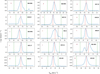 |
Fig. 1 Average C18O (J=2–1) spectrum for 15 different protoclusters. Two vertical green dashed lines indicate the velocity cut-off to measure the systemic velocity (Vsys). The red dashed line represents the measured Vsys based on the C18O (J=2–1) line. In the W51-E and W51-IRS2 regions, the black dashed line indicates the minima between the separation of the two broad clouds. Symbols Y, I, towards and E in the figures denote young, intermediate and evolved protoclusters respectively (see Table 1). |
2.2 Hydrogen column density [N(H2)] and dust temperature (Td) maps
In addition to the C18O (J = 2–1) line, molecular hydrogen column density [N(H2)] and dust temperature (Td) maps have been taken from the work of Dell’Ova et al. (2024). These maps were obtained from point process mapping (PPMAP) analysis, which is based on Bayesian statistics. Using the prior information on the opacity index (κν), dust temperature (Td), and using the resulting spectral energy distribution (SED), the average properties along the line of sight are obtained (Marsh et al. 2006, 2015, 2017). In their analysis, Dell’Ova et al. (2024) used the 1.3 μm continuum, SOFIA/HAWC+ (53 μm, 89 μm, and 214 μm), APEX/SABOCA (350 μm), and APEX/LABOCA (870 μm) data sets. The resulting image cubes for the molecular hydrogen column density map [N(H2)] and dust temperature (Td) maps are at angular resolution of 2.5″. For details, we refer to the work of Dell’Ova et al. (2024).
3 Average spectra of C18O (J = 2–1)
In Fig. 1, we show the average spectra (over the entire field of view) of the C18O (J=2–1) lines for 15 protoclusters. From these spectra, we characterize the systemic velocity (Vsys) for these regions, which are weighted by intensity (see Table 1). In Fig. 1, we indicate the velocity cuts with green dashed lines for each spectrum. We consider the velocity range up to these velocity cuts on both sides of the spectrum to calculate the systemic velocity (Vsys). We indicate the measured intensity-weighted systemic velocity (Vsys = ∑i Iivi/ ∑i Ii, where i is the channel number) for each protocluster with a red dashed line. We note that for calculating Vsys, we consider values that are greater than 3 times the RMS noise (σrms). The null-to-null velocity width for most of the spectra ranges from ~15 to ~30 km s−1. For W43-MM1, W43-MM2 and W43-MM3, we observed cloud components at ~80 km s−1, ~115 km s−1, which were reported as diffuse extended clouds of the W43 complex (Nguyen Luong et al. 2011; Motte et al. 2014). For this reason, we ignore these clouds while calculating the systemic velocity (Vsys) of the protoclusters. In the W51-IRS2 region, we observe two clouds below and above ~55.0 km s−1, which we have marked with a black dashed line in Fig. 1. Due to the presence of two prominent clouds in the average spectra, the Vsys value is not at the peak of the spectra; rather it is slightly shifted from the peak. Likewise, in the W51-E region, we notice two broad clouds below and above 65.0 km s−1, which we have also marked with a black dashed line in Fig. 1. Earlier studies reported these as interacting clouds in W51 complex (Kang et al. 2010; Ginsburg 2017). For this reason, we have taken these clouds into account. The systemic velocities in these 15 regions have already been reported by Motte et al. (2022) based on other surveys conducted in these regions. As we study the C18O (2–1) line, we calculate the systemic velocities (Vsys) in these areas independently. We compare the values with the velocities reported by Motte et al. (2022) and notice that for most regions the difference is below ~2 km s−1. However, Motte et al. (2022) mentioned the same Vsys values for the protoclusters W43-MM1, W43-MM2, and W43-MM3, which are at +97 km s−1. Here we obtain +92.0 and +93.2 km s−1 for the W43-MM2 and W43-MM3 regions. Likewise, for the W51-E and W51-IRS2 regions that reside in the W51 complex, we obtain two different velocities at +57.8 and +59.3 km s−1, respectively. Earlier, Cunningham et al. (2023) examined the Vsys in the 15 protoclusters from the mean line-of-sight values of the DCN (3–2) cores. They also observed similar differences in Vsys between W43-MM1, W43-MM2, and W43-MM3 protoclusters residing in the W43 main complex, and W51-E and W51-IRS2 protoclusters residing in the W51 complex.
4 Moment maps of C18O (J = 2–1) line emission
We show the integrated intensity (moment 0) and integrated intensity-weighted velocity dispersion (moment 2) maps for 15 protoclusters in Figs. 2 and 3. We also show the integrated intensity-weighted peak velocity map (moment 1) for 15 protoclusters in the Appendix A. For calculating the moment maps, we take all the values in each pixel that are above 4.5σrms values. We adopt this cutoff to avoid artefact in the moment maps. In Appendix B, we describe how we calculate the noise value for each pixel. In the W43-MM1 region, we observe a central ridge-shaped structure that may have been the result of the interaction of clouds (Louvet et al. 2016). In the W51-E region, we notice a filament-like structure from south-west (SW) to north-east (NE) direction. In the G008.67 region, we notice two structures. One main structure is in the SW direction in the field of view, and another one is in the NE direction, which is relatively less prominent compared to the former one. Likewise, in the G353.41 region, we notice a filament-like structure from the SW to NE direction (Álvarez-Gutiérrez et al. 2024). In the G333.60 region, we observe two filament-like structures and maybe these structures are formed due to the feedback of the central H II region (Galván-Madrid et al. 2024). In the G010.62 region, we notice spiral arm-like structures which were also observed in the moment 0 map of the DCN (3–2) line (Cunningham et al. 2023). This phenomenon is possibly due to the result of rotation (Liu 2017). In the moment 2 maps in Fig. 3, we also notice a complex structure in the W51-IRS2 region, and the velocity dispersion is relatively high compared to the other regions. For most of the regions, the velocity dispersion values for most pixels lie between 1 and 3 km s−1, whereas in W51-IRS2, the values are between 8 and 10 km s−1. This is possibly due to separate clouds in the same spatial position, which artificially increases the velocity dispersion in the pixels. This is supported by the average spectrum of the C18O line in the W51-IRS2 region (see Section 3). This effect may also be caused in other regions such as G338.93, the central position of G327.29, and the central area of the G010.62 region. For this reason, we calculate the velocity dispersion from the model spectra (obtained after decomposing the spectra into multi-Gaussian components) for analyzing the spatial distribution of Ms in these regions (see Section 5).
5 Estimation of turbulence
We study the turbulence in the protoclusters using two different methods. The first is to use sonic Mach number (Ms) analysis and second one is using size-linewidth relation. To calculate the spatial distribution of Ms in the protoclusters, we require the spatial distribution of the kinetic temperature (Tk) of the gas. As we do not have the direct information of Tk, which is obtained from the analysis of the ammonia spectral line (Pillai et al. 2006; Wang & Wang 2023), we assume that the system is in local thermodynamic equilibrium (LTE) and the gas temperature (Tk) and the dust temperature (Td) are almost the same. This assumption is considerable within the protoclusters and has been considered in previous studies (Sanhueza et al. 2010; Sabatini et al. 2019, 2022). We therefore first smooth the C18O (2–1) image cubes into the same Td images, which are at 2.5″ resolution, and then regrid to the same Td cubes, so that both C18O (2–1) and Td image cubes become identical. After that, we decompose the pixel-wise C18O (2–1) spectra using the Gausspy+ module. To obtain identical image cubes, we use the Python module radio_beam and CASA task imregrid. We note that the spectral resolution in the W43-MM1 region is 0.17 km s−1, whereas in the rest of the regions it is 0.33 km s−1. Therefore, we first smoothed the spectral axis of the W43-MM1 region, so the spectral resolution is 0.34 km s−1, which is similar to the other cubes. We then fit the pixel-wise spectra into multiGaussian components. For extraction of the structure from the position-position-velocity (PPV) cube, we also follow the same procedure in the W43-MM1 region. In the following section, we discuss the fitting procedure using Gausspy+ module.
5.1 Decomposition of spectral profile
Gausspy+ module is based on the automated Gaussian decomposition (AGD) method based on machine learning (Riener et al. 2019). This module is a superior version of the original Gausspy module (Lindner et al. 2015). Using this technique, we can set the maximum jump in the number of components between two neighboring pixels, so that certain jumps in the number of components do not occur. This parameter is called max_jump_comps and in our case we set it to 2. Two smoothing parameters are there called decompose.alpha1 and decompose.alpha2 and these parameters are calculated automatically using some observed spectra. We can set how many spectra it takes to find out these parameters, which is called training.n_spectra. These two smoothing parameters determine the smoothness of the spectrum during the decomposition process. It is important to note that smoothing is spectral smoothing instead of spatial smoothing. It is necessary to make spectral smoothing and derivatives (up to four orders) of the spectra for finding the peak positions of the decomposed components accurately. The original unsmooth spectra are then decomposed based on the guessing of the peak positions from the smoothed spectra. For different types of spectra, e.g., weak and narrow components, it is better to use these two parameters. Otherwise, one smoothing parameter is sufficient to find the components.
The F1 score parameter in the fitting procedure measures the accuracy of the decomposition in the training set. We first mask the pixels whose signal-to-noise ratio (S/N) is below 10 and check the accuracy factor F1 from those spectra. Next, we examine spectra with S/Ns between 10 and 20 and between 20 and 30. We notice that for spectra whose S/N < 10, the accuracy factor drastically drops below 65%. Thus, we first mask pixels whose S/N is less than 10. We have performed this procedure rather than checking the F1 score without any condition because in this way the fit accuracy for lower S/N data is obtained more accurately. Apart from that in some regions, we also notice that below S/N = 10, the spectra are very noisy and the Gausspy+ module fits the spectra with one component. When we plot the spatial distribution of the velocity dispersion, we notice that the outskirts of the region have a drastically increase in velocity dispersion. We then realize that this is due to the decomposition error. Using this cutoff, there is only a very small fraction of total pixels masked in each 2.5″ image cube.
Consequently, after masking those pixels, we fit the pixel-wise spectra into multi-Gaussian components. We finally obtain the peak intensity, center velocity, and full-width-half maximum (FWHM) for each component. We note that the center velocity and the FWHM are in channel number units. Therefore, it is necessary to convert these into velocity units. We can restrict the maximum number of components during the fitting using the parameter max_ncomps. In the work of Riener et al. (2019), it was recommended to set it to ″none″ or to add any value with caution. However, if the line has a major optical depth problem (τν >> 1), after adjusting it to ″none″, it will unnecessarily include multiple components for a single spectrum. Therefore, it is important to examine whether the C18O (2–1) line has a major optical depth (τν) effect. Optical depth of C18O (2–1) line is obtained empirically as a function of the density of the molecular hydrogen column density [N(H2)] from the work of Sabatini et al. (2022), which is log10(τC18O) = 0.6 (log10[N(H2)] −24.0). This relationship was obtained from the study of the infrared dark cloud (IRDC) G014.492-00.13. After assuming the same excitation temperature (Tex) and the filling factor (f) of both C17O (2–1) and C18O (2–1) lines and taking the relationship of the optical depth between C17O (2–1) and C18O (2–1) lines, they fitted pixel-wise spectra and compared the brightness temperature (TB) of the species. From that, they obtained the optical depth map of the C18O (2–1) line. This empirical law was then derived based on the column density map of the hydrogen molecule [N(H2)] and the optical depth (τν) of the C18O (2–1) line. From this law, it is found that for N(H2) = 1023.5 cm−2, τν = 0.50 and for N(H2) = 1024 cm−2, τν = 1.0. Consequently, from the column density maps of hydrogen molecules [N(H2)] of these 15 protoclusters, we also examine the number of pixels with N(H2) > 1023.5 cm−2 or τν > 0.5 and N(H2) > 1024 cm−2 or τν > 1.0. For the case of τν > 0.5, we notice that for most of the protoclusters, it is below 6%; however, in two cases G327.29 and G012.80, these are 12% and 17%, respectively. In the case of τν > 1.0, we noticed that for most protoclusters, it is below 2%; however, in the cases of G012.80 and W51-E, these are 7.8% and 3.0% respectively. Thus, we assumed that the optical depth (τν) does not have a significant impact on the multi-Gaussian fitting. This module contains several other parameters, e.g., significance, snr_noise_spike, refit_rchi2. We have varied these parameters and checked whether these changes affect the final results. However, we did not find any changes in the decomposed spectra. In our analysis, we set the minimum FWHM equal to 2 (in channel number units), which is the minimum criteria for proper sampling of a Gaussian profile. We also check whether noise has an effect on the number of decomposed spectra in these regions, which we discuss in the Appendix C. In addition, we also show some model spectra in Appendix D in the G333.60 region which are obtained from the Gausspy+ module.
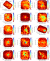 |
Fig. 2 Integrated intensity (moment 0) maps of the C18O (J=2–1) lines for 15 protoclusters. Symbols Y, I, and E in the figures indicate young, intermediate, and evolved protoclusters respectively (see Section 1). |
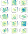 |
Fig. 3 Integrated intensity weighted velocity dispersion (moment 2) maps of the C18O (J=2–1) lines for 15 protoclusters. Symbols Y, I, and E in the figures indicate young, intermediate, and evolved protoclusters respectively (see Section 1). |
5.2 Sonic Mach number (Ms) distribution
After obtaining the pixel-wise decomposed components, we calculate the effective velocity dispersion (σeff) for each pixel using the formula mentioned in Appendix E. We mention that the presence of two isolated components in a pixel artificially increases the velocity dispersion in that pixel, and so is the values for Ms. Thus, we use a different formula for calculating the velocity dispersion in each pixel, which is described in Appendix E. This formula is based on the weight of each component according to their integrated intensity. If multiple Gaussian components are present in a pixel after decomposition of the spectrum, we calculate the effective velocity dispersion (σeff) for that pixel based on the integrated intensity of the components. After calculating the σeff values in each pixel and taking the temperature information from the dust temperature (Td) image, we measure the 1-D nonthermal velocity dispersion (σnth) using the following formula:
![Mathematical equation: $\[\sigma_{\mathrm{nth}}=\sqrt{\sigma_{\mathrm{eff}}^2-\sigma_{\mathrm{th}}^2},\]$](/articles/aa/full_html/2025/10/aa53830-25/aa53830-25-eq1.png) (1)
(1)
where σth is the thermal velocity dispersion equal to ![Mathematical equation: $\[\sqrt{k_{\mathrm{B}} T_{\mathrm{k}} / m_{c^{18} \mathrm{O}}}; k_{\mathrm{B}}\]$](/articles/aa/full_html/2025/10/aa53830-25/aa53830-25-eq2.png) is the Boltzmann constant = 1.38 × 10⁻¹⁶ erg K−1; Tk is the kinetic temperature; mc18O is the mass of the C18O molecule = 30mH, where mH = 1.67 × 10⁻²⁴ g. In our analysis, we assume Td = Tk (see Section 5). We note that the values of Td that we use in our analysis is the molecular hydrogen column density weighted temperature for a single line-of-sight. Likewise, σeff that we calculate for each pixel is also the column density weighted velocity dispersion for a single line-of-sight. Thus, we finally obtain the gas mass-weighted Mach number (Ms) by the formula:
is the Boltzmann constant = 1.38 × 10⁻¹⁶ erg K−1; Tk is the kinetic temperature; mc18O is the mass of the C18O molecule = 30mH, where mH = 1.67 × 10⁻²⁴ g. In our analysis, we assume Td = Tk (see Section 5). We note that the values of Td that we use in our analysis is the molecular hydrogen column density weighted temperature for a single line-of-sight. Likewise, σeff that we calculate for each pixel is also the column density weighted velocity dispersion for a single line-of-sight. Thus, we finally obtain the gas mass-weighted Mach number (Ms) by the formula:
![Mathematical equation: $\[M_{\mathrm{s}}=\frac{\sqrt{3} ~\sigma_{\mathrm{nth}}}{c_{\mathrm{s}}},\]$](/articles/aa/full_html/2025/10/aa53830-25/aa53830-25-eq3.png) (2)
(2)
where cs is the isothermal sound speed equal to ![Mathematical equation: $\[\sqrt{k_{\mathrm{B}} T_{\mathrm{d}} / \mu m_{\mathrm{H}}}\]$](/articles/aa/full_html/2025/10/aa53830-25/aa53830-25-eq4.png) ; μ is the mean molecular weight of the gas = 2.35mH (Ao et al. 2013; Syed et al. 2020; Li et al. 2020). We mention that, when the beam size of the telescope is relatively large, apart from turbulence, other non-thermal effects such as rotation and infall can also broaden the width of the spectral line. However, in our case, the angular resolution is ~0.05 pc (at 2.5″ angular resolution), which is down to the core scale. Consequently, velocity gradients caused by infall or rotation toward the cores are well resolved (Álvarez-Gutiérrez et al. 2024; Sandoval-Garrido et al. 2025). On the other hand, C18O line traces a relatively low density regime compared to other high density tracers such as DCN or N2H+. Thus, infall toward the cores will not significantly affect the linewidth of the C18O line. However, the large-scale velocity gradient may have a significant effect on the linewidth. For that we check the large-scale velocity gradient in the protoclusters on the position-velocity (PV) diagram. We notice that only in the two protoclusters G008.67 and W43-MM1, large velocity gradient is observed in the C18O (2–1) line. We calculate the velocity gradient for these two protoclusters and obtain 1.65 ± 0.01 km s−1 pc−1 for the G008.67 protocluster and 2.99 ± 0.01 km s−1 pc−1 for the W43-MM1 protocluster. The detailed calculation for the velocity gradient is discussed in Appendix F. The distance of the G008.67 protocluster is ~3.4 kpc and the distance of the W43-MM1 protocluster is ~5.5 kpc. Consequently, 2.5″ corresponds to 0.04 pc and 0.06 pc in the G008.67 and W43-MM1 protoclusters, respectively. Now for the ~1.5 km s−1 velocity dispersion of the C18O (2–1) line, it only affects 4 to 11% of the line width. As a result, we assume that the nonthermal component is caused primarily by turbulence rather than large-scale rotation or infall. In addition, we also check whether beam smoothing to 2.5″ resolution has any significant effect on the Mach number analysis. We notice that there is no noticeable effect of beam smoothing. This is further supported by the negligible impact of the large-scale velocity gradient on line width. We discuss this in detail in Appendix G.
; μ is the mean molecular weight of the gas = 2.35mH (Ao et al. 2013; Syed et al. 2020; Li et al. 2020). We mention that, when the beam size of the telescope is relatively large, apart from turbulence, other non-thermal effects such as rotation and infall can also broaden the width of the spectral line. However, in our case, the angular resolution is ~0.05 pc (at 2.5″ angular resolution), which is down to the core scale. Consequently, velocity gradients caused by infall or rotation toward the cores are well resolved (Álvarez-Gutiérrez et al. 2024; Sandoval-Garrido et al. 2025). On the other hand, C18O line traces a relatively low density regime compared to other high density tracers such as DCN or N2H+. Thus, infall toward the cores will not significantly affect the linewidth of the C18O line. However, the large-scale velocity gradient may have a significant effect on the linewidth. For that we check the large-scale velocity gradient in the protoclusters on the position-velocity (PV) diagram. We notice that only in the two protoclusters G008.67 and W43-MM1, large velocity gradient is observed in the C18O (2–1) line. We calculate the velocity gradient for these two protoclusters and obtain 1.65 ± 0.01 km s−1 pc−1 for the G008.67 protocluster and 2.99 ± 0.01 km s−1 pc−1 for the W43-MM1 protocluster. The detailed calculation for the velocity gradient is discussed in Appendix F. The distance of the G008.67 protocluster is ~3.4 kpc and the distance of the W43-MM1 protocluster is ~5.5 kpc. Consequently, 2.5″ corresponds to 0.04 pc and 0.06 pc in the G008.67 and W43-MM1 protoclusters, respectively. Now for the ~1.5 km s−1 velocity dispersion of the C18O (2–1) line, it only affects 4 to 11% of the line width. As a result, we assume that the nonthermal component is caused primarily by turbulence rather than large-scale rotation or infall. In addition, we also check whether beam smoothing to 2.5″ resolution has any significant effect on the Mach number analysis. We notice that there is no noticeable effect of beam smoothing. This is further supported by the negligible impact of the large-scale velocity gradient on line width. We discuss this in detail in Appendix G.
In Fig. 4, we show the spatial distribution and histogram plots of Ms for 15 protoclusters. We note that the values of Ms for all these protoclusters range between ~1 and ~25 with median values ranging from ~5 to ~8 and mean values between ~5 and ~9. The pattern of the histogram plot of Ms is quite similar in all regions. It shows a peak within ~4 to ~7 and extends up to ~25. Although the pattern is quite similar, we did not find any significant increase or decrease in the mean and median values of Ms according to the evolutionary stage of the protoclusters. We also examined whether the distribution of Mach numbers changes after excluding the H II emission and SiO (5–4) outflow regions. However, we did not find any noticeable changes in Mach numbers. As these regions are quite small compared to the field of view, it does not affect the distribution of the Mach number. Moreover, it supports our findings that Mach numbers do not vary according to the evolutionary stage of the protocluster. In two protoclusters, G337.92 and G351.77, there appears to be a slight concentration of Ms in the central region. However, in other cases, we did not find any such effect. The fluctuation of the Mach number is there in the entire field of view.
In Fig. 5, we show the correlation between Ms and σnth, and the correlation between Ms and N(H2) for W43-MM1 protocluster. The rest are shown in Appendix I. For studying the correlation, we first grouped the data in 12 equal intervals according to the values of σnth and N(H2). We note that the number of pixels gradually decreases with increasing N(H2). Thus, the mean and σ values are calculated from fewer data points for higher N(H2). For example, only about 6% pixels contain N(H2) > 1023.5 cm−2 in almost all regions, while it decreases to below 1.8% when N(H2) > 1024 cm−2. From the figure we see that there is no significant correlation between Ms and N(H2) except for the G351.77 region, where a slight correlation is tentatively observed.
We also compare the non-thermal line width and Mach number between C18O line and DCN cores to check whether the turbulence inside the protoclusters varies toward the dense cores. For that, we obtain the velocity dispersion and temperature values of the DCN cores from Cunningham et al. (2023). For our analysis, we only consider the cores fitted with a single Gaussian as mentioned in Cunningham et al. (2023). The number of DCN cores for each protocluster is listed in Table 3. We calculate the mean (and 1 σ dispersion) values of the non-thermal velocity dispersion (σnth, DCN) and the Mach number (Ms, DCN) of DCN cores for each protocluster. We list the values of the non-thermal velocity dispersion (σnth,C18O) and the Mach number (Ms, C18O) calculated from C18O line in Table 3. For calculating σnth, DCN, we take the value of the mass of the DCN molecule as 28mH. We then calculate Ms, DCN from Eq. (2), the same as was calculated for the C18O line (see Table 3). We mention that spectral line observations are broadened by the spectrometer response function (Koch et al. 2018). Earlier studies corrected the channel resolution effect using the formula: ![Mathematical equation: $\[\Delta_{\mathrm{ch}} / 2 \sqrt{2 \ln 2}\]$](/articles/aa/full_html/2025/10/aa53830-25/aa53830-25-eq5.png) , where Δch is the channel resolution of the observation (Li et al. 2020; Barnes et al. 2023). This effect is negligible for the C18O line where the line width is relatively large compared to the DCN line. However, when we check it for the DCN line, we also observe that the average non-thermal velocity dispersion decreases only by 0.02 km s−1 and the average Mach number decreases only by 0.10 from their uncorrected values. Therefore, this correction does not have a significant impact on the final results. From the values of σnth, DCN, we notice that the mean values range between 0.42 and 0.96 and the mean values of Ms, DCN vary between 2.2 and 5.5. We did not find any significant difference according to the evolutionary stage of the protoclusters. Likewise, the mean σnth, C18O ranges from 0.91 to 1.58 and the mean Ms,C18O ranges from 5.3 to 8.7. On average, the mean value of the σnth, DCN and Ms, DCN is almost half that of the C18O values. It indicates that, although turbulence is high in the low density regimes inside the protoclusters, it decreases toward the high density dense cores.
, where Δch is the channel resolution of the observation (Li et al. 2020; Barnes et al. 2023). This effect is negligible for the C18O line where the line width is relatively large compared to the DCN line. However, when we check it for the DCN line, we also observe that the average non-thermal velocity dispersion decreases only by 0.02 km s−1 and the average Mach number decreases only by 0.10 from their uncorrected values. Therefore, this correction does not have a significant impact on the final results. From the values of σnth, DCN, we notice that the mean values range between 0.42 and 0.96 and the mean values of Ms, DCN vary between 2.2 and 5.5. We did not find any significant difference according to the evolutionary stage of the protoclusters. Likewise, the mean σnth, C18O ranges from 0.91 to 1.58 and the mean Ms,C18O ranges from 5.3 to 8.7. On average, the mean value of the σnth, DCN and Ms, DCN is almost half that of the C18O values. It indicates that, although turbulence is high in the low density regimes inside the protoclusters, it decreases toward the high density dense cores.
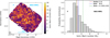 |
Fig. 4 Left: sonic Mach number map in the W43-MM1 protocluster. Right: histogram distribution of the sonic Mach number shown on the left panel. Symbol Y in the figures indicate the young protocluster (see Section 1). We display the remainder of the 15 protoclusters in Appendix H. |
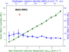 |
Fig. 5 Correlation between (a) the sonic Mach number (Ms) and the non-thermal velocity dispersion (σnth) (green color) and (b) the sonic Mach number (Ms) and the hydrogen column density [N(H2)] (blue color) for W43-MM1. Symbol Y in the figure indicates the young protocluster (see Section 1). We present the reminder of the 15 protoclusters in Appendix I. |
Comparison between the turbulence in the protoclusters obtained from C18O (2–1) lines and the turbulence of the DCN (3–2) cores inside the protoclusters.
5.3 Structure decomposition
An alternative method to determine the nature of turbulence in molecular clouds is to study the relationship between the non-thermal line width with the size of the structures in the protoclusters (Liu et al. 2022; Saha et al. 2022). It is generally believed that interstellar molecular clouds have hierarchical complex structures that range from relatively diffuse structures to dense clumpy structures. These various structures are thought to have been formed by the cascade of eddies generated by interstellar turbulence. Hence, it is essential to extract these structures in order to understand their nature. To accomplish this, we use the Python package astrodendro (Rosolowsky et al. 2008; Shetty et al. 2012), which properly decomposes the structures and provides us with various information such as velocity-dispersion (σtot), area (S), size (Robs), position angle (PA), major (Rmaj) and minor (Rmin) sizes of the structures in the plane of the sky. In the following, we discuss the structure extraction in detail using the astrodendro module.
Using the astrodendro module, the structure is extracted from the position-position-velocity (PPV) cube. After extracting these structures, it computes the intensity-weighted velocity dispersion (σtot) for each structure using the formula:
![Mathematical equation: $\[\sigma_{\mathrm{tot}}=\left[\frac{\sum I_{\mathrm{v}}(\mathrm{v}-\overline{\mathrm{v}})^2}{\sum I_{\mathrm{v}}}\right]^{1 / 2},\]$](/articles/aa/full_html/2025/10/aa53830-25/aa53830-25-eq36.png) (3)
(3)
where ![Mathematical equation: $\[\bar{v}\]$](/articles/aa/full_html/2025/10/aa53830-25/aa53830-25-eq37.png) is the intensity-weighted mean velocity, which is equal to ∑ Ivv/ ∑ Iv. Similarly, it also estimates the major (Rmaj) and minor (Rmin) sizes of the structures (which are ellipses) in the plane of the sky. As an input, we have to insert the PPV cube, from which it extracts the structures. We first calculate the noise map using the line free channels and then convert each velocity channel for each pixel into zero whose amplitude is <2.5σrms. Now, the modified cube represents a cube only with significant fluxes. There are three main parameters that control the extraction of the structure. These are: min_value, min_delta, and min_npix. As we use the modified cube, we set the min_value as close to zero. The second parameter is min_delta. It determines the threshold beyond which it is considered as a structure. We take this value at 2.5σrms. The third parameter is min_npix. This parameter denotes the minimum pixels that are required in the position–position–velocity (x, y, v) space so that it is considered as a single component. We consider minimum 6 channels in the velocity space (v) and for the spatial dimension (x, y), we set the value 2a which is equal to [2π/4ln2].[FWHMx,beam. FWHMy,beam/(pixel_size)2]. Here, FWHMx,beam and FWHMy,beam are the full width at half maximum of the major and minor axes of the beam. After obtaining the Rmaj and Rmin values, we calculate the spherical radius, Robs which is equal to 1.91 times the effective RMS size, Rrms (
is the intensity-weighted mean velocity, which is equal to ∑ Ivv/ ∑ Iv. Similarly, it also estimates the major (Rmaj) and minor (Rmin) sizes of the structures (which are ellipses) in the plane of the sky. As an input, we have to insert the PPV cube, from which it extracts the structures. We first calculate the noise map using the line free channels and then convert each velocity channel for each pixel into zero whose amplitude is <2.5σrms. Now, the modified cube represents a cube only with significant fluxes. There are three main parameters that control the extraction of the structure. These are: min_value, min_delta, and min_npix. As we use the modified cube, we set the min_value as close to zero. The second parameter is min_delta. It determines the threshold beyond which it is considered as a structure. We take this value at 2.5σrms. The third parameter is min_npix. This parameter denotes the minimum pixels that are required in the position–position–velocity (x, y, v) space so that it is considered as a single component. We consider minimum 6 channels in the velocity space (v) and for the spatial dimension (x, y), we set the value 2a which is equal to [2π/4ln2].[FWHMx,beam. FWHMy,beam/(pixel_size)2]. Here, FWHMx,beam and FWHMy,beam are the full width at half maximum of the major and minor axes of the beam. After obtaining the Rmaj and Rmin values, we calculate the spherical radius, Robs which is equal to 1.91 times the effective RMS size, Rrms (![Mathematical equation: $\[\sqrt{R_{\text {maj}} R_{\text {min}}}\]$](/articles/aa/full_html/2025/10/aa53830-25/aa53830-25-eq38.png) ) (Ohno et al. (2023), and references therein). We correct the convolved beam from Robs to obtain the deconvolved size R, which is equal to
) (Ohno et al. (2023), and references therein). We correct the convolved beam from Robs to obtain the deconvolved size R, which is equal to ![Mathematical equation: $\[\sqrt{R_{\text {obs}}^{2}-\theta_{\text {beam}}^{2}}\]$](/articles/aa/full_html/2025/10/aa53830-25/aa53830-25-eq39.png) . Finally, we convert this R into the spatial scale (in pc) after converting the plane-of-sky projected angle into the spatial scale using the source’s distance.
. Finally, we convert this R into the spatial scale (in pc) after converting the plane-of-sky projected angle into the spatial scale using the source’s distance.
We show the correlation between σtot and R for the 15 protoclusters in Fig. 6. The details of the decomposed structures are mentioned in Table 4. σtot versus R is shown in Fig. 6 on a logarithmic scale for better visualization, as the lower end is crowded with a large number of data points. We fit the size-linewidth relation using the Python module scipy.optimize.curvefit. For all cases, the error in the power-law index is either 0.01 or 0.02 and the main error is in the intensity value. Errors in the intensity and power-law index values are rounded up to two decimal places. After obtaining the similar value in the power-law index error, we recheck errors especially in the power-law index using the bootstrapping method. For that, we run 104 samples in each of these regions and randomly select both the velocity dispersion and the length scale and we recover the same results as reported above.
We note that we analyzed the size-linewidth relation at the original angular resolution of the observation. Consequently, in all of these regions, the length scales of the structures vary from ~0.01 pc to ~1.0 pc, with most of them lying below 0.1 pc. This indicates the existence of a relatively large number of small-scale structures inside the protoclusters. The lower and upper length scale limits of the structures are determined by the resolution of the ALMA telescope and the large scale obtained from the spatial extension of this observation, respectively. The number of decomposed structures within these protoclusters varies between 359 and 1945. In the young protoclusters W43-MM1 and W43-MM2, the number of structures is greater than 850. Similarly, for protoclusters G327.29, G328.25, G337.92 and G338.93 the number of structures is greater than 350 but less than 500. Likewise, in the intermediate protoclusters, W43-MM3 and W51-E, the number of structures is above 700, whereas for the other three protoclusters, G008.67, G351.77 and G353.41, the number of structures is below 700. However, in the evolved protoclusters W51-IRS2, G010.62, G012.80, and G333.60, the number of structures varies between 593 and 1945. In G333.60 region, number is structure is 1945 which is relatively large and more than twice the number of structures found in most of the other regions. The possible reason for the relatively large number of structures in G333.60 region could be due to the feedback effect of the H II region, the surrounding environment inside the protoclusters is very complex and small, clumpy structures are produced as a result of this.
In addition, we did not observe any noticeable differences in intensity (A) or power-law index (p) according to the evolutionary stages. Values of A and p of the protoclusters vary between 1.72 and 3.62 and between 0.41 and 0.64, respectively. We note that Astrodendro or any other structure extraction module exhibits a bias with respect to contaminated structures. When extracting small-scale structures (leaves), there is a contamination of large-scale structures (branch and trunk) and vice versa. As a result, large velocity dispersion values are added to the small-scale structures, and vice versa. Therefore, A is higher and p is lower than the original value. Thus, we can say that the fitted A value represents the upper limit and the fitted p value represents the lower limit of the actual value. Apart from the contamination issue, velocity dispersion of the large wing-like structures may reduce significantly due to the value of min_value = 2.5σrms. This is also considered as a caveat in the Astrodendro module. We have checked this effect in Appendix J for four protoclusters. We also point out that velocity dispersion is caused by thermal and non-thermal motions. However, from the analysis of the sonic Mach number (Ms), it is evident that the contribution of the thermal velocity dispersion (σth) is very small. Thus, the thermal velocity dispersion (σth) does not have any significant impact on the intensity (A) and the power-law index (p) of the size-linewidth relation.
We also examined the size-linewidth relation after excluding the H II and SiO (5–4) outflow emission regions. We have taken the polygon regions of H II and SiO (5–4) from previous ALMA-IMF studies (Towner et al. 2024; Galván-Madrid et al. 2024). We check this because in the H II region due to strong stellar radiation, the velocity dispersion is high, which may not be associated with turbulence. In addition, the expansion of the velocity in the outflow region is mainly caused by strong velocity gradients, which may not be the result of turbulence. We check this for the size-linewidth relationship as the structures are extracted from the iso-intensity contours, and thus one isolated intensity structure may cover a significant portion of the outflow or H II region. However, we notice that after excluding these regions, the intensity and the power-law index are similar to the full region analysis and within the 3σ errors of the original. One primary reason is that the C18O (2–1) line emission spreads throughout the field of view of the protoclusters. Consequently, only a small fraction of the area is excluded and does not significantly alter the value of the intensity (A) and the power-law index (p).
Fig. 7 shows the correlation between the size and linewidth of these 15 protoclusters. The blue dots represent structures for young protoclusters, whereas the red and green dots represent structures for intermediate and evolved protoclusters. All three types of protoclusters have the same spatial extent and velocity dispersion values. The total number of structures for young, intermediate, and evolved protoclusters is 3858, 2881, and 4219, respectively. We obtain a fit value of 2.67 ± 0.02 km s−1 and a p value of 0.51 ± 0.00. We also plot the result obtained from the work of Solomon et al. (1987). They studied the PCA analysis of the CO molecule in molecular clouds and obtained the value of A = 1.0 km s−1 and the value of p = 0.50. Although the value of p is similar to our value, the value of A is significantly different from our results. We assume that the discrepancy is mainly caused by the percentage of overlapping structures in the field of view.
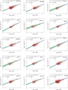 |
Fig. 6 Correlation between velocity dispersion (σtot) and the plane-of-sky projected radius (R) for 15 protoclusters. The red dots represent structures derived using the astrodendro module. The solid blue lines represent the fitted lines for the correlation and the green shaded areas represent the ±3σ regions around the mean fitted values. Symbols Y, I, and E in the figures indicate young, intermediate, and evolved protoclusters respectively (see Section 1). |
Properties of the structures obtained from Astrodendro module.
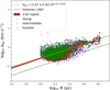 |
Fig. 7 Correlation between velocity dispersion (σtot) and the plane-of-sky projected radius (R) for all 15 protoclusters. Blue, red, and green dots represent the structures for young, intermediate and evolved protoclusters derived using the astrodendro module. The solid orange line represents the fitted line for the correlation and the maroon shaded areas represent the ±3σ regions around the mean fitted value. Black dashed line obtained from the earlier work of Solomon et al. (1987). |
6 Discussion
6.1 Sonic Mach number
In Section 5.2, we studied the sonic Mach number (Ms) in the 15 massive protoclusters. The Ms behaves similarly in all protoclusters, extending up to ~25, with mean and median values ranging from ~5 to ~9 and ~5 to ~8, respectively. Such high levels of turbulence must affect the stellar-formation processes. Moreover, as shown by Motte et al. (2022), these 15 protoclusters span different evolutionary stages among the star-forming process. It seems that turbulence is maintained over time. This could be the effect of feedback processes, such as outflows, supernova explosions, or large-scale galactic interactions (Joung & Mac Low 2006; Agertz et al. 2009; Nony et al. 2023).
It is interesting to note that similar values of Ms were also reported in younger regions, namely in infrared dark clouds (Wang & Wang 2023; Leurini et al. 2011; Dirienzo et al. 2015) and in more evolved regions such as Orion B, a nearby high-mass molecular cloud (Orkisz et al. 2017). Wang & Wang (2023) studied the infrared dark cloud G35.20-0.74 N with the Jansky Very Large Array (JVLA) using emission lines from NH3 (1,1) to (7,7) (similar angular resolution to our Ms analysis). If we convert their sonic Mach number for the three-dimensional system, that is, multiplying their estimates by ![Mathematical equation: $\[\sqrt{3}\]$](/articles/aa/full_html/2025/10/aa53830-25/aa53830-25-eq41.png) , we find the mean, median, and maximum Ms of 6.4, 4.8 and 21.0, respectively. These values are similar to those we obtain in our 15 massive protoclusters. Similarly, Dirienzo et al. (2015) studied infrared dark clouds (IRDC) using NH3 (1,1) and (2,2) lines after combining JVLA and the Green Bank Telescope (GBT) (similar angular resolution to our Ms analysis). They noticed that the turbulence inside the clumps is highly supersonic (with Ms ≈ 5–9), which may support the clumps against gravity. In addition to these studies, Orkisz et al. (2017) examined the turbulence in the nearby high-mass molecular cloud Orion B using various CO isotopes with the IRAM 30 meter telescope. The spatial resolution in this study was 0.05 pc, which is similar to our Ms analysis. They also obtained the histogram plot of Ms similar to our results. The mean value of Ms is ~6.5 and extends to ~20. In addition, they also showed that the distribution of turbulence energy into solenoidal and compressive modes may affect star formation efficiency (SFE). The results of all of these studies, including ours, indicate that turbulence may play a significant role in the dynamics of molecular clouds. Overall, the dynamical effect of turbulence in these 15 protoclusters is beyond the scope of this work. Following the calculation of the magnetic field in these regions, by dust polarization or Zeeman measurements, we will investigate in detail the effect of these opposing forces (magnetic field and turbulence) on gravity inside the protoclusters.
, we find the mean, median, and maximum Ms of 6.4, 4.8 and 21.0, respectively. These values are similar to those we obtain in our 15 massive protoclusters. Similarly, Dirienzo et al. (2015) studied infrared dark clouds (IRDC) using NH3 (1,1) and (2,2) lines after combining JVLA and the Green Bank Telescope (GBT) (similar angular resolution to our Ms analysis). They noticed that the turbulence inside the clumps is highly supersonic (with Ms ≈ 5–9), which may support the clumps against gravity. In addition to these studies, Orkisz et al. (2017) examined the turbulence in the nearby high-mass molecular cloud Orion B using various CO isotopes with the IRAM 30 meter telescope. The spatial resolution in this study was 0.05 pc, which is similar to our Ms analysis. They also obtained the histogram plot of Ms similar to our results. The mean value of Ms is ~6.5 and extends to ~20. In addition, they also showed that the distribution of turbulence energy into solenoidal and compressive modes may affect star formation efficiency (SFE). The results of all of these studies, including ours, indicate that turbulence may play a significant role in the dynamics of molecular clouds. Overall, the dynamical effect of turbulence in these 15 protoclusters is beyond the scope of this work. Following the calculation of the magnetic field in these regions, by dust polarization or Zeeman measurements, we will investigate in detail the effect of these opposing forces (magnetic field and turbulence) on gravity inside the protoclusters.
In addition to the estimation of the Mach number in Section 5.2, we also study the correlation between the Mach number and the hydrogen column density [N(H2)] for 15 massive protoclusters. We notice that there is no significant correlation exists between them. The reason is the C18O line emission traces dense as well as relative low density regimes. The maximum amount of gas, however, appears in the low density regime after including the total power data of ALMA telescope. Thus, in the relatively low density regime probed by C18O line does not have any significant variation in turbulence. However, comparing the non-thermal velocity dispersion values between C18O line and DCN cores, we note that the DCN cores have almost half the non-thermal line width and sonic Mach number compared to the C18O line. It indicates that turbulence decreases toward dense cores. This result is in line with previous studies (Li et al. 2020; Sakai et al. 2022; Wang & Wang 2023; Barnes et al. 2023). For example, Sakai et al. (2022) examined the IRDC G14.492-00.139 with relatively low density tracer C18O (2–1) and several high density tracers such as N2D+ (3–2), DCO+ (3–2), DCN (3–2) toward the dense cores and noticed that low density tracer C18O has almost three times larger line width compared to the high density tracers mentioned above, whose kinematics are associated with dense cores. From their analysis they concluded that a low-density turbulent envelope surrounds less turbulent dense cores. Likewise, in a study by Wang & Wang (2023) showed that most of the cores in the evolved infrared dark cloud G35.20-0.74 N located toward the local minima of the sonic Mach number. In addition, toward the high-mass molecular clouds I18308 and I19220, prestellar cores are formed where the turbulence is mostly transonic, which is low compared to the surrounding molecular clouds where the turbulence is highly supersonic (Lu et al. 2018). Furthermore, in massive infrared dark cloud NGC 6334S, Li et al. (2020) showed that the turbulence in the dense cores is subsonic to transonic. In addition to that, in IRDC G028.37+00.07, Barnes et al. (2023) showed that in dense cores turbulence is transonic in nature. As a consequence, turbulence may not be sufficient to support the cores against gravity unless strong magnetic fields play an important role. In nearby low-mass star-forming molecular clouds such as Taurus, where cores are well resolved, previous studies showed that turbulence decreases toward the periphery of the cores and within the deep interior of the cores, turbulence is subsonic in nature (Goodman et al. 1998; Schnee et al. 2007; Choudhury et al. 2021; Pineda et al. 2021; Koley 2022, 2023a). There are two possible reasons for this. First one is the scale-dependent velocity dispersion of the turbulent eddies. The typical size of the DCN core is ~0.015 pc (Cunningham et al. 2023), whereas the typical size of the C18O (2–1) structures is ~0.05 pc. C18O line traces dense as well as relatively low density regimes which contain larger structures. Therefore, the median values of the size is higher in C18O line compared to DCN line and in turn the larger velocity dispersion. The second one is at the periphery of the prestellar cores, when the effective magnetic Reynolds number (Rm) ~ 1, neutral particles drift through the magnetic field, and due to friction between the neutral particles and the ions, a significant amount of turbulence dissipates (Li & Houde 2008; Stahler & Palla 2004; Hennebelle & Inutsuka 2019). The question of whether the turbulence dissipates in ions or neutral is a matter of debate. Few studies show that turbulence only dissipates in ions at the periphery of the cores. The dissipation of turbulence in neutral occurs at the Kolmogorov scale which is deep inside the core (Li & Houde 2008; Hezareh et al. 2010). As an alternative, few studies have shown that dissipation of turbulence occurs in neutrals rather than ions at the periphery of the core (Pineda et al. 2021, 2024). This is mostly valid in the prestellar cores. The situation for protostellar cores may be complex because of feedback effects of the young protostars. However, previous studies have shown that there is very little difference in the Mach number between starless quiescent cores and protostellar cores (Sánchez-Monge et al. 2013; Barnes et al. 2021).
6.2 Size-linewidth correlation
In addition to the Ms analysis in the protoclusters, we studied the size-linewidth correlation for 15 massive protoclusters individually, which we fit with power-laws (see Section 5.3). We obtained power-law index (p) values ranging from 0.41 to 0.64. There was no significant difference between the evolutionary stages of the protocluster. As we did not find any prominent trend according to the evolutionary stage of the protoclusters, we also plotted the size-linewidth relation after adding all the structures for 15 protoclusters. We obtain that the value of p is 0.51 ±0.00. Previous studies have observed similar values of the power law index in molecular clouds where turbulence is supersonic. For example, Solomon et al. (1987) investigated the size-linewidth relation for 273 molecular clouds using the CO molecular line observed by the Five College Radio Astronomy Observatory (FCRAO). They found that velocity dispersion (σtot) varies with length scale (R) with a value of p = 0.50, which is steeper than 0.38 obtained from the work of Larson (1981). In a similar study using 12CO (J=1–0) line, Heyer & Brunt (2004) reported a size-linewidth relationship for 27 giant molecular clouds and obtained p equal to 0.56. Shetty et al. (2012) studied size-linewidth relations in the dense interstellar medium of the Central Molecular Zone using the tracers such as N2H+, HCN, H13CN, HCO+ and found that the power-law index varies between 0.62 and 0.79. Likewise, Liu et al. (2022) studied the size-linewidth relation in the IRDC G034.43+00.24 using H13CO+ (1–0) line and observed that p = 0.5. Similarly, Rice et al. (2016) studied the size-linewidth relationship of molecular clouds using CO line emissions in the inner and outer Galaxy and found power law index values of 0.52 and 0.49, respectively. In addition, Petkova et al. (2023) studied the Galactic center clouds using HNCO (404−303) line and found that the power-law index is 0.68 ± 0.04, which is identical to their simulated results, which is 0.69 ± 0.03. Furthermore, several other studies have revealed that the power-law index of molecular clouds is steeper than the Kolmogorov law of turbulence (p = 0.33) and varies between 0.50 and 0.70, similar to our study (Kauffmann et al. 2017; Yun et al. 2021; Zhou et al. 2022; Ohno et al. 2023). This value of the power-law index is also obtained from theoretical studies. According to theoretical studies, incompressible hydrodynamic turbulence follows the Kolmogorov scaling relation based on which the nonthermal velocity dispersion (σnth) varies with the length scale with a power-law index (p) of 0.33 (Kolmogorov 1941; Frisch 1995). However, for compressible media, the velocity power law is steeper than the Kolmogorov law of turbulence closer to the Burger law of turbulence, in which the p is around 0.50 (Burgers 1948; Fleck 1983; Kowal & Lazarian 2007; Koley 2023b).
7 Conclusions
In this work, we have studied the turbulence in the 15 massive galactic protoclusters (with masses ~1.0–25.0 × 10³ M⊙ within ~2.5 × 2.5 pc2) observed by the ALMA-IMF Large Program, using the C18O (2–1) emission line. The main findings of this study are as follows:
(1) The probability distribution function (PDF) of the sonic Mach number (Ms) in all these regions exhibits a peak between ~4 and ~7 and extends to ~25. This kind of pattern was also observed in previous studies in high-mass star-forming regions. The values of Ms demonstrate that the turbulence in the density regimes traced by the C18O (2–1) line emission is supersonic in nature. The fluctuations in Mach number are homogeneously distributed within the protoclusters, and we observed no clear differences between the young and the more evolved protoclusters.
(2) We did not find a correlation between Ms and hydrogen column density [N(H2)]. The reason is that the C18O line emission traces dense as well as relative low density environments. However, the maximum amount of gas is spread in the low density regime, which we obtain after including the total power data from the ALMA telescope. Thus, in the relatively low density regime probed by the C18O line does not have any significant variation in turbulence.
(3) We compared the non-thermal line widths of the C18O (2–1) line and the DCN (3–2) cores. They exhibit mean nonthermal line-widths of ~1.2 and ~0.6 km s−1, respectively and mean Mach numbers of ~7.1 and ~3.3 respectively. These observations show a strong decrease in turbulence toward the dense cores.
(4) We extracted the structures (leaves, branches, and truncks) from the position-position-velocity (PPV) cubes of the C18O (2–1) lines using Astrodendro module. The sizelinewidth relations of the structures are well suited by a power law in the form ![Mathematical equation: $\[A(\mathrm{km} \mathrm{~s}^{-1})(\frac{R}{\mathrm{pc}})^{p}\]$](/articles/aa/full_html/2025/10/aa53830-25/aa53830-25-eq42.png) , where A is the intensity and R is the radius of the structure. Among the 15 protoclusters, A and p vary between 1.72 and 3.62 and between 0.41 and 0.64 respectively. We did not find any noticeable increase or decrease in A and p according to the evolutionary stage of the protoclusters. The values of p obtained from this study are steeper than the standard Kolmogorov law of turbulence, as expected for compressible media.
, where A is the intensity and R is the radius of the structure. Among the 15 protoclusters, A and p vary between 1.72 and 3.62 and between 0.41 and 0.64 respectively. We did not find any noticeable increase or decrease in A and p according to the evolutionary stage of the protoclusters. The values of p obtained from this study are steeper than the standard Kolmogorov law of turbulence, as expected for compressible media.
Overall, with this work we have examined the turbulence of 15 massive protoclusters using C18O (2–1) and DCN (3–2) lines. We notice that turbulence in the relatively low density regime traced by C18O line is relatively higher compared to the high density DCN cores. In the future, this study will help provide a better understanding of the role of turbulence in molecular clouds.
Acknowledgements
We greatly acknowledge to the referee for helping us to improve the manuscript significantly. This paper makes use of the following ALMA data: ADS/JAO.ALMA 2017.1.01355.L. ALMA is a partnership of ESO (representing its member states), NSF (USA) and NINS (Japan), together with NRC (Canada), MOST and ASIAA (Taiwan), and KASI (Republic of Korea), in co-operation with the Republic of Chile. The Joint ALMA Observatory is operated by ESO, AUI/NRAO and NAOJ. The project leading to this publication has received support from ORP, which is funded by the European Union’s Horizon 2020 research and innovation program under grant agreement No. 101004719 [ORP]. This project has received funding from the European Research Council (ERC) via the ERC Synergy Grant ECOGAL (grant 855130) and from the French Agence Nationale de la Recherche (ANR) through the project COSMHIC (ANR-20-CE31-0009). A.K. would like to thank Guido Garay for useful discussions during the 2nd Center of Excellence in Astrophysics and Related Technologies (CATA) annual meeting held on Santiago, Chile in 2023. A.K. and L.B. gratefully acknowledge support from ANID BASAL project FB210003. A.K. would also like to acknowledge Fondecyt postdoctoral fellowship (project id: 3250070, 2025). A.S. gratefully acknowledges support by the Fondecyt Regular (project code 1220610), and ANID BASAL project FB210003. R.A. gratefully acknowledges support from ANID Beca Doctorado Nacional 21200897. P.S. was partially supported by a Grant-in-Aid for Scientific Research (KAKENHI Number JP22H01271 and JP23H01221) of JSPS. R.G.M. acknowledges support from UNAM-PAPIIT project IN108822 and from CONAHCyT Ciencia de Frontera project ID 86372. Part of this work was performed at the high-performance computers at IRyA-UNAM. T.C. and M.B. have received financial support from the French State in the framework of the IdEx Université de Bordeaux Investments for the future Program. A.G. acknowledges support from the NSF under grants AST 2008101 and CAREER 2142300. M.B. is a postdoctoral fellow in the University of Virginia’s VICO collaboration and is funded by grants from the NASA Astrophysics Theory Program (grant number 80NSSC18K0558) and the NSF Astronomy & Astrophysics program (grant number 2206516). G.B. acknowledges support from the PID2023-146675NB-100 (MCI-AEI-FEDER,UE) program. H.-L. Liu is supported by Yunnan Fundamental Research Project (grant No. 202301AT070118, 202401AS070121). This work is supported by the China-Chile Joint Research Fund (CCJRF No. 2312). CCJRF is provided by Chinese Academy of Sciences South America Center for Astronomy (CASSACA) and established by National Astronomical Observatories, Chinese Academy of Sciences (NAOC) and Chilean Astronomy Society (SOCHIAS) to support China-Chile collaborations in astronomy. Telescope: the Atacama Large Millimeter/submillimeter Array (ALMA). Software: Astropy (Astropy Collaboration 2013), CASA (Common Astronomy Software Applications package-National Radio Astronomical Observatory) (version 6.5.1.23) (McMullin et al. 2007), Matplotlib (Hunter 2007), Gausspy+ (Riener et al. 2019), Astrodendro (Rosolowsky et al. 2008).
Appendix A Integrated intensity weighted velocity (moment 1) maps of 15 massive protoclusters
We show the integrated intensity weighted velocity (moment 1) maps for 15 massive protoclusters in Fig. A.1. We note that all the moment 1 maps have been constructed by subtracting the systemic velocity (Vsys), which result in a more prominent appearance of the clouds with negative and positive velocity (with respect to the Vsys). We will study these maps in the upcoming C18O (2–1) kinematic paper (Koley et al. in prep).
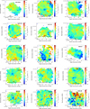 |
Fig. A.1 Integrated intensity weighted velocity (moment 1) maps of the C18O (J=2–1) lines for 15 protoclusters. Symbols Y, I, and E in the figures indicate young, intermediate, and evolved protoclusters respectively (see Section 1). |
Appendix B Noise estimation
The noise distribution is calculated for 15 regions using the line-free channels. We take the maximum line-free channels and calculate the noise for each pixel in the region. In Fig. B.1, we show the noise distribution maps for G008.67 and G353.41 regions. The noise level is almost constant in the central areas and gradually increases as one moves toward the edge. This is caused by the spatial variation in the sensitivity of the primary beam. These maps are scaled-up versions of their corresponding primary beam response functions (.pb image cube produced during CASA task TCLEAN). In Table 2, we mention the noise values for each protocluster, which are based on the central portion of the noise maps, where the level of noise is almost constant.
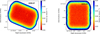 |
Fig. B.1 Left figure: Noise map (per channel) of the G008.67 region. Right figure: Noise map (per channel) of the G353.41 region. |
Appendix C Examining the effect of noise on the number of decomposed components
We examine whether the level of noise affects the number of decomposed components in these regions. For this purpose, we choose one protocluster G010.62. In this region, we first decompose the pixel-wise spectra using the original noise map and obtain the distribution of the number of components (n). We then carefully check the original noise map and include random noise in each pixel of the model cube or noise free data cube. The noise value that has been included in each pixel of the model cube is obtained from the edge side of the original noise map. As an example, in the upper panel of Fig. C.1, we illustrate the noise map and the number of decomposed components (n) of the G010.62 region. The number of maximum Gaussian components (n) in the central region of G010.62 is four and decreases toward the edge where the value of n is one. We check the noise map and notice that the value of the noise toward the central region is ~0.035 Jy beam−1 and the gradually increases toward the the edge side, where it is ~ 0.053 Jy beam−1. We take this noise value from the edge side and include it in each pixel of the model cube and create a data cube. In this data cube, the noise in each pixel is 0.053 Jy beam−1. Thereafter, we decompose that cube into multi-Gaussian components with the same signal-to-noise (S/N) cutoff as was done for the original one and obtain the distribution of the number of components (n) in this region. The constant noise map and the resulting distribution of the components are displayed on the left and right sides of the lower panel of Fig. C.1. We now compare the distribution of n for both the cases and notice that due to the increase in noise, the number of components in a few regions is less compared to the original one. Consequently, our conclusion is that the increase in the number of components toward the center of the protocluster and the decrease toward the outer side may not always be physical, but may also be related to the level of noise.
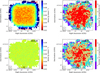 |
Fig. C.1 Upper-left figure: Noise map of the G010.62 region (at 2.5″ resolution, same as the dust temperature cube). Upper-right figure: Distribution of number of decomposed components (n) in the G010.62 region. Lower-left figure: Constant noise map at ~0.053 Jy beam−1. Lower-right figure: Distribution of number of decomposed components (n) when the noise level in each pixel is equal to ~0.053 Jy beam−1. |
Appendix D Model spectra in G333.60 region
We have shown a few samples of model spectra in Fig. D.1 in the region of G333.60. Here, the observed C18O (J = 2–1) spectra are indicated by black solid lines, while decomposed spectra and the model spectra are indicated by red solid lines. We have also shown the residuals for each of the spectra.
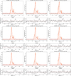 |
Fig. D.1 Few samples of model C18O (J = 2–1) spectra toward G333.60 region obtained from Gausspy+ module. First, third, and fifth rows show the observed and model C18O (J = 2–1) spectra in G333.60 region. Black solid line denotes the observed spectra, whereas, red sold lines represent the decomposed and resultant model spectra in G333.60 region. In each of the figures two red dotted horizontal lines denote the ±1σ value of the noise. In addition one solid horizontal red line represents the +3σ noise level of the spectra. In the header of each of the figures idx represents the spectra number that is obtained from the Gausspy+ module. X and Y denote the pixel number in the image cube, Ncomp is the number of decomposed components and |
![Mathematical equation: $\[\chi_{\text {red }}^{2}\]$](/articles/aa/full_html/2025/10/aa53830-25/aa53830-25-eq43.png)
Appendix E Integrated intensity weighted velocity dispersion
The traditional intensity-weighted velocity dispersion (σv) of a position-position-velocity (PPV) image cube is obtained by:
![Mathematical equation: $\[\sigma_{\mathrm{v}}=\sqrt{\frac{\sum_i I_i\left(v_i-M_1\right)^2 ~d v_i}{\sum_i I_i ~d v_i}},\]$](/articles/aa/full_html/2025/10/aa53830-25/aa53830-25-eq44.png) (E.1)
(E.1)
here, Ii is the intensity of the ith channel, M1 is the intensity-weighted center velocity (moment 1) map of the spectra. M1 is calculated by the formula:
![Mathematical equation: $\[M_1=\frac{\sum_i I_i v_i ~d v_i}{\sum_i I_i ~d v_i},\]$](/articles/aa/full_html/2025/10/aa53830-25/aa53830-25-eq45.png) (E.2)
(E.2)
however, σv does not represent the effective velocity dispersion for a spectra when the spectra contains multiple components and these components are separated from each other or more specifically they are disjoint components. In this case, it will always overestimate the σv from the original value. For this reason, after obtaining the decomposed model components using Gausspy+ module, we calculate the effective velocity dispersion (σeff) by the formula:
![Mathematical equation: $\[\sigma_{\mathrm{eff}}=\sqrt{\frac{\sum_i I_{i, 1}\left(v_{i, 1}-v_{c, 1}\right)^2 ~d v_{i, 1}+\sum_i I_{i, 2}\left(v_{i, 2}-v_{c, 2}\right)^2 ~d v_{i, 2}+\ldots \ldots}{\sum_i I_{i, 1} ~d v_{i, 1}+\sum_i I_{i, 2} ~d v_{i, 2}+\ldots \ldots}}\]$](/articles/aa/full_html/2025/10/aa53830-25/aa53830-25-eq46.png) (E.3)
(E.3)
![Mathematical equation: $\[\sigma_{\mathrm{eff}}=\sqrt{\frac{\sum_i I_{i, 1}\left(v_{i, 1}-v_{c, 1}\right)^2 ~d v_{i, 1}}{\sum_i I_{i, 1} ~d v_{i, 1}+\sum_i I_{i, 2} ~d v_{i, 2}+\ldots \ldots}+\frac{\sum_i I_{i, 2}\left(v_{i, 2}-v_{c, 2}\right)^2 ~d v_{i, 2}}{\sum_i I_{i, 1} ~d v_{i, 1}+\sum_i I_{i, 2} ~d v_{i, 2}+\ldots \ldots}+\ldots \ldots}\]$](/articles/aa/full_html/2025/10/aa53830-25/aa53830-25-eq47.png) (E.4)
(E.4)
![Mathematical equation: $\[\sigma_{\text {eff }}=\sqrt{\left(\frac{\sum_i I_{i, 1} ~d v_{i, 1}}{\sum_i I_{i, 1} ~d v_{i, 1}+\sum_i I_{i, 2} ~d v_{i, 2}~+..}\right)\left(\frac{\sum_i I_{i, 1}\left(v_{i, 1}-v_{c, 1}\right)^2 ~d v_{i, 1}}{\sum_i I_{i, 1} ~d v_{i, 1}}\right)+\left(\frac{\sum_i I_{i, 2} ~d v_{i, 2}}{\sum_i I_{i, 1} ~d v_{i, 1}+\sum_i I_{i, 2} ~d v_{i, 2}~+..}\right)\left(\frac{\sum_i I_{i, 2}\left(v_{i, 2}-v_{c, 2}\right)^2 ~d v_{i, 2}}{\sum_i I_{i, 2} ~d v_{i, 2}}\right)+..}\]$](/articles/aa/full_html/2025/10/aa53830-25/aa53830-25-eq48.png) (E.5)
(E.5)
![Mathematical equation: $\[\sigma_{\mathrm{eff}}=\sqrt{\left(\frac{w_1}{w} ~\sigma_1^2+\frac{w_2}{w} ~\sigma_2^2~+..\right)},\]$](/articles/aa/full_html/2025/10/aa53830-25/aa53830-25-eq49.png) (E.6)
(E.6)
where Ii,1, Ii,2 are the intensities of the first and second components for the ith channel; vi,1, vi,2 are the velocities of the first and second components for the ith channel; vc,1, vc,2 are the center velocities of the first and second components; ![Mathematical equation: $\[w=\left({\sum}_{i, 1} ~I_{i, 1} ~d v_{i, 1}+{\sum}_{i, 2} ~I_{i, 2} ~d v_{i, 2}~+~..\right)=\]$](/articles/aa/full_html/2025/10/aa53830-25/aa53830-25-eq50.png) total integrated intensity; w1 = ∑i,1 Ii,1 dvi,1 = integrated intensity of the first component; w2 = ∑i,2 Ii,2 dvi,2 = integrated intensity of the second component; σ1 and σ2 are the intensity-weighted velocity dispersion for the first and second components. Previously, Pan et al. (2023) used a similar kind of formula for effective velocity dispersion to avoid overestimation of velocity dispersion. However, it was not exactly the same as our effective velocity dispersion (σeff).
total integrated intensity; w1 = ∑i,1 Ii,1 dvi,1 = integrated intensity of the first component; w2 = ∑i,2 Ii,2 dvi,2 = integrated intensity of the second component; σ1 and σ2 are the intensity-weighted velocity dispersion for the first and second components. Previously, Pan et al. (2023) used a similar kind of formula for effective velocity dispersion to avoid overestimation of velocity dispersion. However, it was not exactly the same as our effective velocity dispersion (σeff).
In the average spectra of two regions, W51-E and W51-IRS2, we observed broad separate clouds (see Section 3). In these regions, we observe a prominent overestimation of velocity dispersion if we calculate it using Eqn. E.1 instead of Eqn. E.6. In Fig. E.1, we show the ratio of σeff and σv for these two regions and notice that for most pixels the ratio is below 0.50.
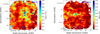 |
Fig. E.1 Left figure: Ratio of the effective velocity dispersion (σeff) and the traditional velocity dispersion (σv) for W51-E region. Right figure: Ratio of the effective velocity dispersion (σeff) and the traditional velocity dispersion (σv) for W51-IRS2 region. |
Appendix F Calculation of position-velocity (PV) diagram toward an inclined angle
In a few cases, we notice that integrated intensity structures (moment 0 map) are inclined on the plane of the sky rather than toward the vertical or horizontal direction on the sky plane. Therefore, to study the position-velocity (PV) diagram properly, it was necessary to rotate the axes in parallel and perpendicular directions of the integrated intensity maps. In the following, we have outlined the necessary steps that were required to do this with an example shown in Figure F.1. Suppose that an integrated intensity structure (shown in orange color) is present on the sky plane with an inclination angle θ with respect to the horizontal axis (Right Ascension). If one rotates this structure with an angle −θ, the structure looks similar to the violet dashed line, and the pixel positions of the lower left corner and the upper right corner are x_initial_0, y_initial_0 and x_final, y_final respectively. The increment between two successive pixels along the horizontal and vertical directions of the image plane is Δx and Δy. To obtain the information of the equidistant points within the inclined intensity structure (which are mentioned with red solid squares), we increase the pixel value successively from the lower left corner in two directions, which are parallel and perpendicular of the inclined structure. These directions are indicated by green and blue color arrows.
We start from the lower left hand pixel x_initial_0, y_initial_0 and count all the pixels round[x_initial_0+Δy.cos(90+θ),y_initial_0+Δy.sin(90+θ)] by increasing Δy with one unit from 0 to (y_final - y_initial_0). After that, we change the initial pixel value: x_initial_0 → x_initial_0+Δx.cos(θ) and y_initial_0 → y_initial_0+Δx.sin(θ) and count all the equidistant points as before. This same procedure goes on and each time the initial pixel value is modified by increasing the Δx with unity and this step will go on up to (x_final - x_initial_0). In this way all the equidistant points that are enclosed within the inclined intensity structure are counted.
We calculated the large-scale velocity gradient in 15 protoclusters using the above procedure. First, we decompose the pixel-wise spectra into multi-Gaussian components. After that we create image planes for center velocities and the integrated intensities for each of the components. Then we plot the center velocities of all of these components in two different directions. We give the color of each component according to its integrated intensity. We performed this analysis for all 15 protoclusters by varying the inclination angle from 0 to 360°. However, only in two protoclusters G008.67 and W43-MM1, we obtain a large-scale velocity gradient. These are shown in Figures F.2 and F.3. While fitting, we give more weight to the components with high integrated intensities. The velocity gradients that we obtain are 1.95 ± 0.01 and 2.99 ± 0.01 km s−1 pc−1 for these two protoclusters. We fitted velocity gradients up to half of the image plane in the W43-MM1 protocluster because after that point there is no prominent velocity gradient observed.
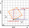 |
Fig. F.1 Inclined (with an angle θ) integrated intensity structure (orange square) on the two dimensional image plane. The same integrated intensity structure shown in violet dashed line when rotate with an angle − θ. The red solid squares are the pixels which are enclosed within the inclined integrated intensity. Green and red arrows denote the two directions parallel and perpendicular to the inclined structure. |
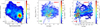 |
Fig. F.2 Left figure is the integrated intensity map (moment 0) of the G008.67 region obtained from 2.5″ circular beam. Here, the orange rectangular region denotes the area where we examine the position-velocity (PV) diagram in two perpendicular directions (toward the green and red arrows). Middle figure is the intensity weighted PV diagram toward the direction of the green arrow mentioned in the left figure. Right figure is the intensity weighted PV diagram toward the direction of the red arrow mentioned in the left figure. Color bars in the Middle and Right figures denotes the integrated intensity of the components. The fitted velocity gradient is 1.95 ± 0.01 km s−1 pc−1 which is shown in red solid color. |
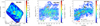 |
Fig. F.3 Left figure is the integrated intensity (moment 0) map of W43-MM1 region obtained from 2.5″ circular beam. Here, the orange rectangular region denotes the area where we examine the position-velocity (PV) diagram in two perpendicular directions (toward the green and red arrows). Middle figure is the intensity weighted PV diagram toward the direction of the green arrow mentioned in the left figure. Right figure is the intensity weighted PV diagram toward the direction of the red arrow mentioned in the left figure. Color bars in the Middle and Right figures denote the integrated intensity of the components. The fitted velocity gradient is 2.99 ± 0.01 km s−1 pc−1 which is shown in red solid color. |
Appendix G Examining the effect of spatial smoothing on Sonic Mach number (Ms) distribution in G337.92 protocluster
For calculating the sonic Mach number (Ms) distribution in these 15 protoclusters, we required to smooth the C18O (2–1) line cubes into the same dust image cubes which are at a slightly coarser angular resolution at 2.5″ (Dell’Ova et al. 2024). Consequently, we examine whether beam smoothing has a significant impact on the sonic Mach number (Ms) analysis. We tested this using one protocluster G337.92 whose original beam size was 0.70″ × 0.55″. First, we fit the pixel-wise spectra using the Gausspy+ module and calculate the effective velocity dispersion (σeff) using the Eqn. E.6. We show the spatial distribution and histogram plot of σeff in the upper left and right panels of Fig. G.1. From the right panel, we notice that the median and the mean values are 0.96 and 1.11 respectively. The distribution also extends up to ~5. Then, we smooth the original C18O (2–1) line image cube with a circular beam of 2.5″ and fit the pixel-wise spectra with the same Gausspy+ module. In the lower left and right panels of Fig. G.1, we show the spatial distribution and the histogram plots of the sonic mach number (Ms) distribution at the 2.5″ circular beam. From the histogram plot, we notice that the median and mean values are 0.93 and 1.11 respectively. Here also the distribution extends up to ~5. From the comparison of the histogram plots in two beam sizes, we notice that due to the beam smoothing, the values of σeff are not significantly affected, which indicates that there has been an insignificant effect on the sonic Mach number (Ms) analysis. Maybe, significantly large beam smoothing (>> 2.5″) will have a noticeable impact on the distribution of σeff. Therefore, in our study, we first smooth all the regions with 2.5″ beam and study the sonic mach number (Ms) distribution.
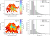 |
Fig. G.1 Upper left and right figures are the spatial distribution and the histogram plot of the effective velocity dispersion (σeff) in G337.92 region when the beam size is 0.70″ × 0.55″. Lower left and right figures are the spatial distribution and the histogram plot of the effective velocity dispersion (σeff) in G337.92 region when the beam size is 2.5″ × 2.5″. |
Appendix H Distribution of Sonic Mach number (Ms) in the protoclusters
We show the spatial distribution and histogram plot of Ms for the protoclusters in Fig.H.1.
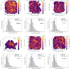 |
Fig. H.1 For each protocluster, we display the map of the sonic Mach number (color map) and the histogram plot of its distribution below. Symbols Y and I in figures indicate the young and intermediate stage protoclusters (see Section 1. |
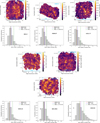 |
Fig. H.2 Continuation of Fig. H.1. . Symbols I and E in figures indicate the intermediate and evolved protoclusters (see Section 1. |
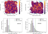 |
Fig. H.3 Sonic Mach (continued). Symbol E in figures indicates the evolved protoclusters (see Section 1. |
Appendix I Correlation between sonic Mach number (Ms) and hydrogen column density [N(H2)] for the protoclusters
We show the correlation between sonic Mach number (Ms) and hydrogen column density [N(H2)] for protoclusters in Fig. I.1
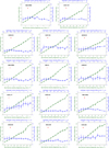 |
Fig. I.1 Correlation between (a) the sonic Mach number (Ms) and the non-thermal velocity dispersion (σnth) (green color) and (b) the sonic Mach number (Ms) and hydrogen column density [N(H2)] (blue color) for protoclusters. Symbols Y, I, and E in the figures indicate the young, intermediate, and evolved protoclusters (see Section 1). |
Appendix J Examining the effect of an intensity cut (min_value = 2.5σrms) on the velocity dispersion (σtot) of the wider lines in the dendogram analysis
We checked whether the parameter min_value in the Astrodendro module reduced the velocity dispersion of the wider components. While extracting the structures from the PPV cube, we set min_value to 2.5σrms for all the protoclusters. On the one hand, it is necessary to avoid taking noise in the analysis; on the other hand, this criterion may truncate a significant fraction of the large wing for the broad components. Currently, there is no effective way to resolve this issue. However, we have checked for four protoclusters whether this effect is severe or not. The four protoclusters are W43-MM1, G333.60, G338.93, and W51-E. In Fig. J.1., we first plot the histogram of the FWHM of the C18O (2–1) line components that we obtain from the Gausspy+ module. From the figures, it shows that the histogram plots of the FWHM for the number of components exhibit a log-normal type profile. The FWHMs extend up to ~16 km s−1 in all four cases. We set the cut-off point for FWHM at 5 km s−1, beyond which we consider the components to have wings-like structures. Although this cut-off point is somewhat arbitrary, there is no way to set any absolute value. We then plot the histogram of the components whose FWHM is greater than 5 km s−1 into two categories. One for which the peak intensity of the components is greater than 3 × min_value and the other for which the peak intensity of the components is below 3 × min_value. These histograms are plotted for four protoclusters in blue and red colors on the right panels of Fig. J.1. From these figures, it indicates that between 6 and 10 km s−1, components of which Ipeak is > 3 × min_value are dominated compared to the number of components for which Ipeak is < 3 × min_value. However, beyond ~10 km s−1, the number of components in two categories becomes more or less equal. Consequently, due to the cutoff of min_value = 2.5σrms, the FWHM of half of the larger components whose FWHM is greater than 10 km s−1 may reduce significantly. This can be considered as a caveat for the Astrodendro module, in addition to the contamination issue of the structures.
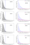 |
Fig. J.1 Left panel in four rows show the histogram plots of the full-width-half-maximum (FWHM) of the C18O (2–1) line components for the W43-MM1, G333.60, G338.93, and W51-E protoclusters respectively. Here the blue dashed line denotes the FWHM value of 5.0 km s−1, above which we consider the components have large wing-like structures. Right panel in four rows show the histogram plots of the components for the four protoclusters whose FWHM are above 5.0 km s−1 and intensity peaks (Ipeak) are above 3× min_value (blue color) and below 3× min_value (red color). |
References
- Agertz, O., Lake, G., Teyssier, R., et al. 2009, MNRAS, 392, 294 [NASA ADS] [CrossRef] [Google Scholar]
- Álvarez-Gutiérrez, R. H., Stutz, A. M., Law, C. Y., et al. 2021, ApJ, 908, 86 [CrossRef] [Google Scholar]
- Álvarez-Gutiérrez, R. H., Stutz, A. M., Sandoval-Garrido, N., et al. 2024, A&A, 689, A74 [NASA ADS] [CrossRef] [EDP Sciences] [Google Scholar]
- Ao, Y., Henkel, C., Menten, K. M., et al. 2013, A&A, 550, A135 [NASA ADS] [CrossRef] [EDP Sciences] [Google Scholar]
- Armante, M., Gusdorf, A., Louvet, F., et al. 2024, A&A, 686, A122 [NASA ADS] [CrossRef] [EDP Sciences] [Google Scholar]
- Astropy Collaboration (Robitaille, T. P., et al.) 2013, A&A, 558, A33 [NASA ADS] [CrossRef] [EDP Sciences] [Google Scholar]
- Barnes, A. T., Henshaw, J. D., Fontani, F., et al. 2021, MNRAS, 503, 4601 [CrossRef] [Google Scholar]
- Barnes, A. T., Liu, J., Zhang, Q., et al. 2023, A&A, 675, A53 [NASA ADS] [CrossRef] [EDP Sciences] [Google Scholar]
- Bonfand, M., Csengeri, T., Bontemps, S., et al. 2024, A&A, 687, A163 [NASA ADS] [CrossRef] [EDP Sciences] [Google Scholar]
- Brouillet, N., Despois, D., Molet, J., et al. 2022, A&A, 665, A140 [NASA ADS] [CrossRef] [EDP Sciences] [Google Scholar]
- Burgers, J. 1948, in Advances in Applied Mechanics, 1, A Mathematical Model Illustrating the Theory of Turbulence, eds. R. Von Mises, & T. Von Kármán (Elsevier), 171 [Google Scholar]
- Busquet, G., Estalella, R., Palau, A., et al. 2016, ApJ, 819, 139 [Google Scholar]
- Choudhury, S., Pineda, J. E., Caselli, P., et al. 2021, A&A, 648, A114 [NASA ADS] [CrossRef] [EDP Sciences] [Google Scholar]
- Csengeri, T., Bontemps, S., Wyrowski, F., et al. 2017, A&A, 601, A60 [NASA ADS] [CrossRef] [EDP Sciences] [Google Scholar]
- Cunningham, N., Ginsburg, A., Galván-Madrid, R., et al. 2023, A&A, 678, A194 [NASA ADS] [CrossRef] [EDP Sciences] [Google Scholar]
- Dell’Ova, P., Motte, F., Gusdorf, A., et al. 2024, A&A, 687, A217 [NASA ADS] [CrossRef] [EDP Sciences] [Google Scholar]
- Dewangan, L. K. 2022, MNRAS, 513, 2942 [Google Scholar]
- Dirienzo, W. J., Brogan, C., Indebetouw, R., et al. 2015, AJ, 150, 159 [Google Scholar]
- Federrath, C. 2015, MNRAS, 450, 4035 [Google Scholar]
- Federrath, C. 2018, Phys. Today, 71, 38 [NASA ADS] [CrossRef] [Google Scholar]
- Federrath, C., & Klessen, R. S. 2012, ApJ, 761, 156 [Google Scholar]
- Fleck, R. C. J., 1983, ApJ, 272, L45 [Google Scholar]
- Frisch, U. 1995, Turbulence. The legacy of A.N. Kolmogorov [Google Scholar]
- Galván-Madrid, R., Díaz-González, D. J., Motte, F., et al. 2024, ApJS, 274, 15 [CrossRef] [Google Scholar]
- Ginsburg, A. 2017, arXiv e-prints [arXiv:1702.06627] [Google Scholar]
- Ginsburg, A., Csengeri, T., Galván-Madrid, R., et al. 2022, A&A, 662, A9 [NASA ADS] [CrossRef] [EDP Sciences] [Google Scholar]
- Goodman, A. A., Barranco, J. A., Wilner, D. J., & Heyer, M. H. 1998, ApJ, 504, 223 [Google Scholar]
- Green, A., Wong, T., Indebetouw, R., et al. 2024, ApJ, 966, 51 [Google Scholar]
- Hacar, A., Alves, J., Burkert, A., & Goldsmith, P. 2016, A&A, 591, A104 [NASA ADS] [CrossRef] [EDP Sciences] [Google Scholar]
- He, Y.-X., Liu, H.-L., Tang, X.-D., et al. 2023, ApJ, 957, 61 [NASA ADS] [CrossRef] [Google Scholar]
- Hennebelle, P., & Inutsuka, S.-i. 2019, Front. Astron. Space Sci., 6, 5 [Google Scholar]
- Heyer, M. H., & Brunt, C. M. 2004, ApJ, 615, L45 [NASA ADS] [CrossRef] [Google Scholar]
- Hezareh, T., Houde, M., McCoey, C., & Li, H.-b. 2010, ApJ, 720, 603 [Google Scholar]
- Hofner, P., Wyrowski, F., Walmsley, C. M., & Churchwell, E. 2000, ApJ, 536, 393 [Google Scholar]
- Hunter, J. D. 2007, Comput. Sci. Eng., 9, 90 [NASA ADS] [CrossRef] [Google Scholar]
- Joung, M. K. R., & Mac Low, M.-M. 2006, ApJ, 653, 1266 [NASA ADS] [CrossRef] [Google Scholar]
- Kang, M., Bieging, J. H., Kulesa, C. A., et al. 2010, ApJS, 190, 58 [Google Scholar]
- Kauffmann, J., Pillai, T., Zhang, Q., et al. 2017, A&A, 603, A89 [NASA ADS] [CrossRef] [EDP Sciences] [Google Scholar]
- Koch, E., Rosolowsky, E., & Leroy, A. K. 2018, RNAAS, 2, 220 [NASA ADS] [Google Scholar]
- Koley, A. 2019, MNRAS, 483, 593 [CrossRef] [Google Scholar]
- Koley, A. 2022, MNRAS, 516, 185 [NASA ADS] [CrossRef] [Google Scholar]
- Koley, A. 2023a, PASA, 40, e053 [Google Scholar]
- Koley, A. 2023b, PASA, 40, e046 [Google Scholar]
- Koley, A., Roy, N., Menten, K. M., et al. 2021, MNRAS, 501, 4825 [Google Scholar]
- Koley, A., Roy, N., Momjian, E., Sarma, A. P., & Datta, A. 2022, MNRAS, 516, L48 [NASA ADS] [CrossRef] [Google Scholar]
- Kolmogorov, A. 1941, Akad. Nauk SSSR Dok1., 30, 301 [Google Scholar]
- Kong, S., Arce, H. G., Carpenter, J. M., et al. 2021, AJ, 161, 229 [NASA ADS] [CrossRef] [Google Scholar]
- Kowal, G., & Lazarian, A. 2007, ApJ, 666, L69 [NASA ADS] [CrossRef] [Google Scholar]
- Larson, R. B. 1981, MNRAS, 194, 809 [Google Scholar]
- Leurini, S., Pillai, T., Stanke, T., et al. 2011, A&A, 533, A85 [NASA ADS] [CrossRef] [EDP Sciences] [Google Scholar]
- Li, H.-b., & Houde, M. 2008, ApJ, 677, 1151 [NASA ADS] [CrossRef] [Google Scholar]
- Li, S., Zhang, Q., Liu, H. B., et al. 2020, ApJ, 896, 110 [Google Scholar]
- Lindner, R. R., Vera-Ciro, C., Murray, C. E., et al. 2015, AJ, 149, 138 [NASA ADS] [CrossRef] [Google Scholar]
- Liu, H. B. 2017, A&A, 597, A70 [NASA ADS] [CrossRef] [EDP Sciences] [Google Scholar]
- Liu, H.-L., Stutz, A., & Yuan, J.-H. 2019, MNRAS, 487, 1259 [Google Scholar]
- Liu, H.-L., Tej, A., Liu, T., et al. 2022, MNRAS, 511, 4480 [NASA ADS] [CrossRef] [Google Scholar]
- Louvet, F., Motte, F., Gusdorf, A., et al. 2016, A&A, 595, A122 [NASA ADS] [CrossRef] [EDP Sciences] [Google Scholar]
- Louvet, F., Sanhueza, P., Stutz, A., et al. 2024, A&A, 690, A33 [NASA ADS] [CrossRef] [EDP Sciences] [Google Scholar]
- Lu, X., Zhang, Q., Liu, H. B., et al. 2018, ApJ, 855, 9 [Google Scholar]
- Mac Low, M.-M., & Klessen, R. S. 2004, Rev. Mod. Phys., 76, 125 [Google Scholar]
- Mallick, K. K., Sharma, S., Dewangan, L. K., et al. 2023, J. Astrophys. Astron., 44, 34 [Google Scholar]
- Mangum, J. G., & Shirley, Y. L. 2015, PASP, 127, 266 [Google Scholar]
- Marsh, K. A., Velusamy, T., & Ware, B. 2006, AJ, 132, 1789 [NASA ADS] [CrossRef] [Google Scholar]
- Marsh, K. A., Whitworth, A. P., & Lomax, O. 2015, MNRAS, 454, 4282 [Google Scholar]
- Marsh, K. A., Whitworth, A. P., Lomax, O., et al. 2017, MNRAS, 471, 2730 [Google Scholar]
- McMullin, J. P., Waters, B., Schiebel, D., Young, W., & Golap, K. 2007, in Astronomical Society of the Pacific Conference Series, 376, Astronomical Data Analysis Software and Systems XVI, eds. R. A. Shaw, F. Hill, & D. J. Bell, 127 [Google Scholar]
- Melchior, A.-L., & Combes, F. 2016, A&A, 585, A44 [NASA ADS] [CrossRef] [EDP Sciences] [Google Scholar]
- Menon, S. H., Federrath, C., Klaassen, P., Kuiper, R., & Reiter, M. 2021, MNRAS, 500, 1721 [Google Scholar]
- Motte, F., Nguyên Luong, Q., Schneider, N., et al. 2014, A&A, 571, A32 [NASA ADS] [CrossRef] [EDP Sciences] [Google Scholar]
- Motte, F., Nony, T., Louvet, F., et al. 2018, Nat. Astron., 2, 478 [Google Scholar]
- Motte, F., Bontemps, S., Csengeri, T., et al. 2022, A&A, 662, A8 [NASA ADS] [CrossRef] [EDP Sciences] [Google Scholar]
- Motte, F., Pouteau, Y., Nony, T., et al. 2025, A&A, 694, A24 [NASA ADS] [CrossRef] [EDP Sciences] [Google Scholar]
- Myers, P. C. 1983, ApJ, 270, 105 [Google Scholar]
- Nakano, T. 1998, ApJ, 494, 587 [NASA ADS] [CrossRef] [Google Scholar]
- Nguyen Luong, Q., Motte, F., Schuller, F., et al. 2011, A&A, 529, A41 [NASA ADS] [CrossRef] [EDP Sciences] [Google Scholar]
- Nishimura, A., Tokuda, K., Kimura, K., et al. 2015, ApJS, 216, 18 [NASA ADS] [CrossRef] [Google Scholar]
- Nony, T., Motte, F., Louvet, F., et al. 2020, A&A, 636, A38 [NASA ADS] [CrossRef] [EDP Sciences] [Google Scholar]
- Nony, T., Galván-Madrid, R., Motte, F., et al. 2023, A&A, 674, A75 [NASA ADS] [CrossRef] [EDP Sciences] [Google Scholar]
- Ohno, T., Tokuda, K., Konishi, A., et al. 2023, ApJ, 949, 63 [NASA ADS] [CrossRef] [Google Scholar]
- Orkisz, J. H., Pety, J., Gerin, M., et al. 2017, A&A, 599, A99 [NASA ADS] [CrossRef] [EDP Sciences] [Google Scholar]
- Palau, A., Zhang, Q., Girart, J. M., et al. 2021, ApJ, 912, 159 [NASA ADS] [CrossRef] [Google Scholar]
- Pan, S., Liu, H.-L., & Qin, S.-L. 2023, MNRAS, 519, 3851 [NASA ADS] [Google Scholar]
- Paron, S., Areal, M. B., & Ortega, M. E. 2018, A&A, 617, A14 [NASA ADS] [CrossRef] [EDP Sciences] [Google Scholar]
- Petkova, M. A., Kruijssen, J. M. D., Henshaw, J. D., et al. 2023, MNRAS, 525, 962 [Google Scholar]
- Pillai, T., Wyrowski, F., Menten, K. M., & Krügel, E. 2006, A&A, 447, 929 [NASA ADS] [CrossRef] [EDP Sciences] [Google Scholar]
- Pineda, J. E., Schmiedeke, A., Caselli, P., et al. 2021, ApJ, 912, 7 [NASA ADS] [CrossRef] [Google Scholar]
- Pineda, J. E., Soler, J. D., Offner, S., et al. 2024, A&A, 690, L5 [NASA ADS] [CrossRef] [EDP Sciences] [Google Scholar]
- Pouteau, Y., Motte, F., Nony, T., et al. 2022, A&A, 664, A26 [NASA ADS] [CrossRef] [EDP Sciences] [Google Scholar]
- Rawat, V., Samal, M. R., Eswaraiah, C., et al. 2024, MNRAS, 528, 1460 [Google Scholar]
- Reyes-Reyes, S. D., Stutz, A. M., Megeath, S. T., et al. 2024, MNRAS, 529, 2220 [NASA ADS] [CrossRef] [Google Scholar]
- Rice, T. S., Goodman, A. A., Bergin, E. A., Beaumont, C., & Dame, T. M. 2016, ApJ, 822, 52 [Google Scholar]
- Riener, M., Kainulainen, J., Henshaw, J. D., et al. 2019, A&A, 628, A78 [NASA ADS] [CrossRef] [EDP Sciences] [Google Scholar]
- Rosolowsky, E. W., Pineda, J. E., Kauffmann, J., & Goodman, A. A. 2008, ApJ, 679, 1338 [Google Scholar]
- Sabatini, G., Giannetti, A., Bovino, S., et al. 2019, MNRAS, 490, 4489 [Google Scholar]
- Sabatini, G., Bovino, S., Sanhueza, P., et al. 2022, ApJ, 936, 80 [NASA ADS] [CrossRef] [Google Scholar]
- Saha, A., Tej, A., Liu, H.-L., et al. 2022, MNRAS, 516, 1983 [NASA ADS] [CrossRef] [Google Scholar]
- Sakai, T., Sanhueza, P., Furuya, K., et al. 2022, ApJ, 925, 144 [NASA ADS] [CrossRef] [Google Scholar]
- Sánchez-Monge, Á., Palau, A., Fontani, F., et al. 2013, MNRAS, 432, 3288 [CrossRef] [Google Scholar]
- Sandoval-Garrido, N. A., Stutz, A. M., Álvarez-Gutiérrez, R. H., et al. 2025, A&A, 696, A202 [NASA ADS] [CrossRef] [EDP Sciences] [Google Scholar]
- Sanhueza, P., Garay, G., Bronfman, L., et al. 2010, ApJ, 715, 18 [Google Scholar]
- Sanhueza, P., Liu, J., Morii, K., et al. 2025, ApJ, 980, 87 [Google Scholar]
- Schnee, S., Caselli, P., Goodman, A., et al. 2007, ApJ, 671, 1839 [NASA ADS] [CrossRef] [Google Scholar]
- Shetty, R., Beaumont, C. N., Burton, M. G., Kelly, B. C., & Klessen, R. S. 2012, MNRAS, 425, 720 [Google Scholar]
- Solomon, P. M., Rivolo, A. R., Barrett, J., & Yahil, A. 1987, ApJ, 319, 730 [Google Scholar]
- Stahler, S. W., & Palla, F. 2004, The Formation of Stars [Google Scholar]
- Stutz, A. M. 2018, MNRAS, 473, 4890 [NASA ADS] [CrossRef] [Google Scholar]
- Stutz, A. M., & Gould, A. 2016, A&A, 590, A2 [NASA ADS] [CrossRef] [EDP Sciences] [Google Scholar]
- Syed, J., Wang, Y., Beuther, H., et al. 2020, A&A, 642, A68 [NASA ADS] [CrossRef] [EDP Sciences] [Google Scholar]
- Towner, A. P. M., Ginsburg, A., Dell’Ova, P., et al. 2024, ApJ, 960, 48 [NASA ADS] [CrossRef] [Google Scholar]
- Ungerechts, H., Bergin, E. A., Goldsmith, P. F., et al. 1997, ApJ, 482, 245 [Google Scholar]
- Wang, C., & Wang, K. 2023, A&A, 674, A46 [NASA ADS] [CrossRef] [EDP Sciences] [Google Scholar]
- Wang, J.-W., Koch, P. M., Galván-Madrid, R., et al. 2020, ApJ, 905, 158 [Google Scholar]
- Yun, H.-S., Lee, J.-E., Evans, Neal J., I., et al. 2021, arXiv e-prints [arXiv:2107.13323] [Google Scholar]
- Zhou, J.-X., Li, G.-X., & Chen, B.-Q. 2022, MNRAS, 513, 638 [NASA ADS] [CrossRef] [Google Scholar]
All Tables
Comparison between the turbulence in the protoclusters obtained from C18O (2–1) lines and the turbulence of the DCN (3–2) cores inside the protoclusters.
All Figures
|
Fig. 1 Average C18O (J=2–1) spectrum for 15 different protoclusters. Two vertical green dashed lines indicate the velocity cut-off to measure the systemic velocity (Vsys). The red dashed line represents the measured Vsys based on the C18O (J=2–1) line. In the W51-E and W51-IRS2 regions, the black dashed line indicates the minima between the separation of the two broad clouds. Symbols Y, I, towards and E in the figures denote young, intermediate and evolved protoclusters respectively (see Table 1). |
| In the text | |
|
Fig. 2 Integrated intensity (moment 0) maps of the C18O (J=2–1) lines for 15 protoclusters. Symbols Y, I, and E in the figures indicate young, intermediate, and evolved protoclusters respectively (see Section 1). |
| In the text | |
|
Fig. 3 Integrated intensity weighted velocity dispersion (moment 2) maps of the C18O (J=2–1) lines for 15 protoclusters. Symbols Y, I, and E in the figures indicate young, intermediate, and evolved protoclusters respectively (see Section 1). |
| In the text | |
|
Fig. 4 Left: sonic Mach number map in the W43-MM1 protocluster. Right: histogram distribution of the sonic Mach number shown on the left panel. Symbol Y in the figures indicate the young protocluster (see Section 1). We display the remainder of the 15 protoclusters in Appendix H. |
| In the text | |
|
Fig. 5 Correlation between (a) the sonic Mach number (Ms) and the non-thermal velocity dispersion (σnth) (green color) and (b) the sonic Mach number (Ms) and the hydrogen column density [N(H2)] (blue color) for W43-MM1. Symbol Y in the figure indicates the young protocluster (see Section 1). We present the reminder of the 15 protoclusters in Appendix I. |
| In the text | |
|
Fig. 6 Correlation between velocity dispersion (σtot) and the plane-of-sky projected radius (R) for 15 protoclusters. The red dots represent structures derived using the astrodendro module. The solid blue lines represent the fitted lines for the correlation and the green shaded areas represent the ±3σ regions around the mean fitted values. Symbols Y, I, and E in the figures indicate young, intermediate, and evolved protoclusters respectively (see Section 1). |
| In the text | |
|
Fig. 7 Correlation between velocity dispersion (σtot) and the plane-of-sky projected radius (R) for all 15 protoclusters. Blue, red, and green dots represent the structures for young, intermediate and evolved protoclusters derived using the astrodendro module. The solid orange line represents the fitted line for the correlation and the maroon shaded areas represent the ±3σ regions around the mean fitted value. Black dashed line obtained from the earlier work of Solomon et al. (1987). |
| In the text | |
|
Fig. A.1 Integrated intensity weighted velocity (moment 1) maps of the C18O (J=2–1) lines for 15 protoclusters. Symbols Y, I, and E in the figures indicate young, intermediate, and evolved protoclusters respectively (see Section 1). |
| In the text | |
|
Fig. B.1 Left figure: Noise map (per channel) of the G008.67 region. Right figure: Noise map (per channel) of the G353.41 region. |
| In the text | |
|
Fig. C.1 Upper-left figure: Noise map of the G010.62 region (at 2.5″ resolution, same as the dust temperature cube). Upper-right figure: Distribution of number of decomposed components (n) in the G010.62 region. Lower-left figure: Constant noise map at ~0.053 Jy beam−1. Lower-right figure: Distribution of number of decomposed components (n) when the noise level in each pixel is equal to ~0.053 Jy beam−1. |
| In the text | |
|
Fig. D.1 Few samples of model C18O (J = 2–1) spectra toward G333.60 region obtained from Gausspy+ module. First, third, and fifth rows show the observed and model C18O (J = 2–1) spectra in G333.60 region. Black solid line denotes the observed spectra, whereas, red sold lines represent the decomposed and resultant model spectra in G333.60 region. In each of the figures two red dotted horizontal lines denote the ±1σ value of the noise. In addition one solid horizontal red line represents the +3σ noise level of the spectra. In the header of each of the figures idx represents the spectra number that is obtained from the Gausspy+ module. X and Y denote the pixel number in the image cube, Ncomp is the number of decomposed components and |
| In the text | |
|
Fig. E.1 Left figure: Ratio of the effective velocity dispersion (σeff) and the traditional velocity dispersion (σv) for W51-E region. Right figure: Ratio of the effective velocity dispersion (σeff) and the traditional velocity dispersion (σv) for W51-IRS2 region. |
| In the text | |
|
Fig. F.1 Inclined (with an angle θ) integrated intensity structure (orange square) on the two dimensional image plane. The same integrated intensity structure shown in violet dashed line when rotate with an angle − θ. The red solid squares are the pixels which are enclosed within the inclined integrated intensity. Green and red arrows denote the two directions parallel and perpendicular to the inclined structure. |
| In the text | |
|
Fig. F.2 Left figure is the integrated intensity map (moment 0) of the G008.67 region obtained from 2.5″ circular beam. Here, the orange rectangular region denotes the area where we examine the position-velocity (PV) diagram in two perpendicular directions (toward the green and red arrows). Middle figure is the intensity weighted PV diagram toward the direction of the green arrow mentioned in the left figure. Right figure is the intensity weighted PV diagram toward the direction of the red arrow mentioned in the left figure. Color bars in the Middle and Right figures denotes the integrated intensity of the components. The fitted velocity gradient is 1.95 ± 0.01 km s−1 pc−1 which is shown in red solid color. |
| In the text | |
|
Fig. F.3 Left figure is the integrated intensity (moment 0) map of W43-MM1 region obtained from 2.5″ circular beam. Here, the orange rectangular region denotes the area where we examine the position-velocity (PV) diagram in two perpendicular directions (toward the green and red arrows). Middle figure is the intensity weighted PV diagram toward the direction of the green arrow mentioned in the left figure. Right figure is the intensity weighted PV diagram toward the direction of the red arrow mentioned in the left figure. Color bars in the Middle and Right figures denote the integrated intensity of the components. The fitted velocity gradient is 2.99 ± 0.01 km s−1 pc−1 which is shown in red solid color. |
| In the text | |
|
Fig. G.1 Upper left and right figures are the spatial distribution and the histogram plot of the effective velocity dispersion (σeff) in G337.92 region when the beam size is 0.70″ × 0.55″. Lower left and right figures are the spatial distribution and the histogram plot of the effective velocity dispersion (σeff) in G337.92 region when the beam size is 2.5″ × 2.5″. |
| In the text | |
|
Fig. H.1 For each protocluster, we display the map of the sonic Mach number (color map) and the histogram plot of its distribution below. Symbols Y and I in figures indicate the young and intermediate stage protoclusters (see Section 1. |
| In the text | |
|
Fig. H.2 Continuation of Fig. H.1. . Symbols I and E in figures indicate the intermediate and evolved protoclusters (see Section 1. |
| In the text | |
|
Fig. H.3 Sonic Mach (continued). Symbol E in figures indicates the evolved protoclusters (see Section 1. |
| In the text | |
|
Fig. I.1 Correlation between (a) the sonic Mach number (Ms) and the non-thermal velocity dispersion (σnth) (green color) and (b) the sonic Mach number (Ms) and hydrogen column density [N(H2)] (blue color) for protoclusters. Symbols Y, I, and E in the figures indicate the young, intermediate, and evolved protoclusters (see Section 1). |
| In the text | |
|
Fig. J.1 Left panel in four rows show the histogram plots of the full-width-half-maximum (FWHM) of the C18O (2–1) line components for the W43-MM1, G333.60, G338.93, and W51-E protoclusters respectively. Here the blue dashed line denotes the FWHM value of 5.0 km s−1, above which we consider the components have large wing-like structures. Right panel in four rows show the histogram plots of the components for the four protoclusters whose FWHM are above 5.0 km s−1 and intensity peaks (Ipeak) are above 3× min_value (blue color) and below 3× min_value (red color). |
| In the text | |
Current usage metrics show cumulative count of Article Views (full-text article views including HTML views, PDF and ePub downloads, according to the available data) and Abstracts Views on Vision4Press platform.
Data correspond to usage on the plateform after 2015. The current usage metrics is available 48-96 hours after online publication and is updated daily on week days.
Initial download of the metrics may take a while.