| Issue |
A&A
Volume 702, October 2025
|
|
|---|---|---|
| Article Number | A248 | |
| Number of page(s) | 16 | |
| Section | Extragalactic astronomy | |
| DOI | https://doi.org/10.1051/0004-6361/202556347 | |
| Published online | 28 October 2025 | |
Constraining the origin of the long-term periodicity of FRB 20180916B with polarization position angle
1
Max-Planck-Institute for Radio Astronomy, Auf dem Hügel 69, Bonn 53121, Germany
2
Department of Astrophysical Sciences, Princeton University, Princeton, NJ 08544, USA
3
National Centre for Radio Astrophysics, Ganeshkhind, Tata Institute of Fundamental Research, Post Bag 3, Pune – 411 007, India
4
Department of Physics, McGill University, 3600 rue University, Montréal, QC H3A 2T8, Canada
5
Trottier Space Institute, McGill University, 3550 rue University, Montréal QC H3A 2A7, Canada
⋆ Corresponding author: This email address is being protected from spambots. You need JavaScript enabled to view it.
Received:
10
July
2025
Accepted:
1
September
2025
Abstract
Context. The repeating fast radio burst (FRB) FRB 20180916B produces bursts in a 5.1 day active window that repeats with a 16.34 day period. Models have been proposed to explain the periodicity using dynamical phenomena of neutron stars such as rotation, precession, or orbital motion. The polarization position angle (PA) of the bursts can be used to distinguish and constrain the origin of the long-term periodicity of the FRB.
Aims. We aim to study the PA variability on short (within an observation) and long timescales (from observation to observation). Given the periodicity of the source, we also study the PA variations within the active window and across multiple windows. Then, we compare the observed PA variability with the predictions of various dynamical progenitor models for the FRB.
Methods. We used the calibrated burst dataset detected by uGMRT in Band 4 (650 MHz) published in our earlier work. We transformed the PA measured at 650 MHz to infinite frequency such that PAs measured in different observations are consistent, and finally we measured the changes within and across active windows.
Results. We find that the PA of the bursts varies according to the periodicity of the source. We constrained the PA variability to be less than seven degrees on timescales less than four hours for all MJDs. We also tentatively find that the PA varies within an active window with a variability of a few degrees per hour. In addition, we tentatively note the PA measured at the same phase in the active window varies from one cycle to another.
Conclusions. Using the findings, we constrained the rotational, precession, and binary progenitor models involving compact objects, where the emission originates from the magnetosphere of the compact object. The rotational model partially agrees with the observed PA variability, but it requires further study to be fully constrained. We robustly rule out all flavors of precessional models where the precession of a neutron star either explains the periodicity of the FRB or the variability from one cycle to another. We can rule out the relativistic spin precession binary model. Lastly, we observed similarities between FRB 20180916B and an X-ray binary system, Her X 1, and explicitly note that the two sources exhibit a similar form of PA variability.
Key words: methods: observational / techniques: polarimetric
© The Authors 2025
 Open Access article, published by EDP Sciences, under the terms of the Creative Commons Attribution License (https://creativecommons.org/licenses/by/4.0), which permits unrestricted use, distribution, and reproduction in any medium, provided the original work is properly cited.
This article is published in open access under the Subscribe to Open model.
Open access funding provided by Max Planck Society.
1. Introduction
Fast radio bursts (FRBs) are short duration transient events that occur in the radio regime of the electromagnetic spectrum (Lorimer et al. 2007; Petroff et al. 2019, 2022; Bailes 2022). FRB 20180916B (CHIME/FRB Collaboration 2019) is a repeating FRB source that emits bursts within a window that is (i) periodic, with a period of 16.34 days (Chime/Frb Collaboration 2020), and (ii) chromatic such that it shifts in time and varies in duration with observing frequency (Pastor-Marazuela et al. 2021; Pleunis et al. 2021; Bethapudi et al. 2023). Even with over 100 activity windows having been observed since the discovery of FRB 20180916B, there has been no measurable change in period (Sand et al. 2023; Lan et al. 2024). Published bursts of FRB 20180916B across wide frequencies exhibit a flat or unchanging position angle (PA) over burst timescales (Nimmo et al. 2021; Pastor-Marazuela et al. 2021; Pleunis et al. 2021; Bethapudi et al. 2023; Mckinven et al. 2023; Sand et al. 2022; Gopinath et al. 2024). Moreover, the rotation measure (RM) of the FRB has been known to vary in a step-like fashion (Mckinven et al. 2023; Gopinath et al. 2024; Bethapudi et al. 2025; Ng et al. 2025). The causes for periodicity, chromaticity, lack of any variability in period, and step-like variability in RM is not known. There have been many progenitor models to explain FRB 20180916B (Levin et al. 2020; Zanazzi & Lai 2020; Beniamini et al. 2020; Wada et al. 2021). A subset of those models explain periodicity using some form of dynamics such as rotation, precession, or binary motion. Collectively, these models are referred to as dynamical models. Each dynamical model has its own geometry and predicts unique temporal variability of PA on short and long timescales. We took inspiration from Li & Zanazzi (2021) and studied the temporal PA variations and compared what is observed and what is predicted by the various dynamical models. In this way, we hope to understand the geometry of the system and produce novel knowledge about the source.
The PA of the polarized light measures its orientation with respect to the plane of the sky. If the nature of emission is such that the PA is tied to the geometry of the system, then by studying the PA variations, we can track the geometric variations. Such insights into geometry have already been demonstrated through study of the PA variations of pulsars. Pulsars are fast spinning neutron stars, and they emit electromagnetic radiation, primarily in radio (Lorimer & Kramer 2012). The radio emission is thought to originate from the open magnetic field lines of its dipolar magnetic field. The open field lines co-rotate with the spinning neutron star. Therefore, the PA of the emission shows the imprint of the co-rotation. This imprint is modeled with the rotating vector model (hereafter RVM; Radhakrishnan & Cooke 1969; Everett & Weisberg 2001). Recent works, such as Johnston et al. (2023, 2024), have shown that RVM can explain the observed PA sweep in over 80% of the pulsars in the Thousand-Pulsar-Array program (Johnston et al. 2020). Moreover, long-term studies of PAs of pulsars and magnetars (highly magnetized neutron stars; Kaspi & Beloborodov 2017) have elucidated novel geometrical phenomena. For instance, Desvignes et al. (2019) performed RVM modeling of PA data of a binary pulsar system PSR J1906+0746 over a time span of 10 years and measured drift of the spin axis due to relativistic spin precession. Similarly, Meng et al. (2024) studied the relativistic spin precession of a double neutron star system PSR J1946+2052 using PA data collected over 3 years. Additionally, by fitting RVMs to PA data of magnetar XTE 1810-197 at different MJDs, Desvignes et al. (2024) reported how the magnetar relaxes its internal structure over the course of several days after X-ray burst activity. Clearly, long-term modeling of PA data enables study of the geometric variations exhibited by the emitting body, provided the PA tracks the geometry.
Features seen in PAs of FRBs could also be indicative of geometry, but connecting the PAs of the FRBs to a geometry has not been straightforward. So far, RVM modeling has only been attempted with few non-repeating FRBs that display “informative” (non-flat) PA sweeps. FRB 20221022A is a non-repeating FRB detected by CHIME/FRB, which presented an S-curve-like PA sweep similar to what is predicted by RVM (Mckinven et al. 2024). Furthermore, Mckinven et al. (2024) have performed RVM modeling assuming different duty cycles and attempted to constrain the geometry. In addition, Bera et al. (2024) has reported the discovery of a non-repeating FRB, FRB 20210912A, by ASKAP that exhibits PA variations between its two sub-components. Bera et al. (2024) tried to explain the variation by fitting RVM to the PA time series. However, such a geometric origin need not always be the case. For example, Bera et al. (2025) describe two non-repeating FRBs whose polarization features evolve within burst duration, possibly indicating a plasma birefringent propagation medium. In this case, the variation of the PA does not need to exclusively track the geometry. However, such exotic polarization features and propagating media are uncommon in FRBs, and FRB 20180916B does not exhibit any of such features. Significantly, a long-term study of PAs of repeating FRBs has not yet been attempted, but with this paper, we attempt to conduct such a study with FRB 20180916B. In Sect. 2, we describe the collection of bursts and all the analysis steps we performed to accurately measure PA, which can be compared between observations. We study the variability of PA across various timescales and measure the rates of the variability in Sect. 3. We compare the observer PA variability with that predicted by the dynamical models in Sect. 4. Lastly, we present our discussions and conclusions in Sect. 5 and Sect. 6, respectively.
2. Data and analysis
This section describes all the data processing steps taken to measure PAs of the bursts. All the bursts were detected with the uGMRT (Swarup 1991; Gupta et al. 2017) in Band 4 (550–750 MHz) with Phased Array mode of operation, the details of which can be found in Bethapudi et al. (2025) (hereafter SB24). Table 1 of SB24 lists all the observations and number of bursts per each observation. It also lists various auxiliary sources, such as noise diode, quasars and known pulsars, which have been used in flux/polarization calibration and testing the performance of the search pipeline. In this paper, we show the activity phase, the number of bursts and the maximum time separation among bursts per each observation in Table 1. We use the periodicity model presented in Sand et al. (2023) to compute activity cycle and activity phase of the bursts. That is, we use reference MJD of 58369.4 and period of 16.34 days. Activity phase is a number between 0 and 1, which linearly maps to the period. Activity cycle is the integer number of periods elapsed since the reference MJD. We first convert the bursts from PSRFITS to TIMER format using PAM (Hotan et al. 2004). Then, we apply the calibration solutions as derived in SB24 using PAC, which also performs parallactic angle correction. From hereon, we only refer to the calibrated burst archive in TIMER format.
Measured properties from every observation.
2.1. PA calibration
The PAs are measured with respect to the sky frame. To meaningfully compare PAs measured from different observations, PA measurements have to be in the same sky frame. Therefore, we need to perform PA calibration so that PA measurements of a some known source with known and fixed PA from different observations are consistent and representative of the true PA value. This is usually achieved using polarized quasars, such as 3C138 and 3C286, whose PAs are modeled and fitted for as a function of observing frequency (Perley & Butler 2013). However, we do not have multiple observations when 3C138 was observed. Therefore, we employed a different strategy here. We make use of known pulsars, PSR B0329+54 and PSR J0139+5814, to perform PA calibration. That is, we make use of PA-sweeps of the pulsars to perform PA calibration. Our choice of using pulsars and not standard quasars implies our PA measurements although consistent among themselves, are not in any absolute frame as defined in Perley & Butler (2013). That is, we have only taken care of inter-observation PA offsets, and there may be a global PA offset which would bring them into the absolute reference frame of Perley & Butler (2013). Naturally, PA calibration and thus further analysis was only done with those observations where we observed either of the two pulsars.
As our PA references, we used the European Pulsar Network Database (EPNDB) 610 MHz pulse profiles of PSR B0329+541 and PSR J0139+58142. We fold all the B0329+54 and J0139+5814 scans (see Table 1, auxiliary sources column SB24) using DSPSR (van Straten & Bailes 2011) and calibrate using the same procedure and calibration solution we used to calibrate the bursts from the respective observations. We also used same QU-fitting procedure (SB24) to estimate RM and also correct for it using PAM. Then, we phase align all the pulsar archives with their corresponding EPNDB reference pulse profile. We do the phase alignment by minimizing the cross-correlation between Stokes-I integrated profiles. Now, measuring position angle correction is simply a matter of measuring the offset in the position angle sweep of the observed pulsar with respect to the reference PA sweep.
In the end, there can only be one PA reference. The EPNDB pulsar profiles of PSR B0329+54 and PSR J0139+5814 need not be in the same reference frame themselves and have to be brought to the same frame. To do so, we note that we have four observations (MJD 59274, MJD 59275, MJD 59944, MJD 59993) where we have scans of both of the test pulsars. We measure PA corrections from each of the test pulsars from all the four observations, which are tabulated in Table A.1. We note that the difference between the PA corrections found using PSR B0329+54 and PSR J0139+5814 is consistent with mean of 42.50 and standard deviation of 1.75 deg. This consistency in the difference across multiple MJDs strongly convinces us that (i) PAs can be calibrated, and (ii) a single PA reference can be constructed using either of the test pulsars. Therefore, we set EPNDB PSR B0329+54 as our main reference and correct EPNDB PSR J1039+5814 by 42.5 deg so that it agrees with the PA frame of EPNDB PSR B0329+54. Then, for all the observations where we use PSR J0139+5814 to do PA calibration, we use this corrected EPNDB PSR J0139+5814. We show the phase-aligned Stokes-I and PA calibrated PA-sweeps for each of the pulsar scans from different observations in Figure A.1. The reference source and the corrections for each observation are shown in Source and Correction columns of Table 1.
Lastly, we note that PSR B0329+54 has a complicated PA sweep and also is seen to undergo mode changes within our dataset. Moreover, its peak linear polarization fraction is not high. However, we note that for all the observations where we use PSR B0329+54 for PA calibration, the Stokes-I profile and the PA-sweep agree well (see Figure A.1). In hindsight, PSR B0329+54 might not have been an ideal choice. Nevertheless, we are confident in our consistent position angle measurements and leave to a future work on acquiring absolute position angles.
2.2. Measuring RM
When light passes through an ionized medium with magnetic fields threading along the propagating direction, the PA of light undergoes rotation. This effect is known as Faraday rotation. It is mathematically understood as
 (1)
(1)
where λ is the wavelength of light, PA∞ is the PA measured at ∞ frequency (or also the initial PA), and PAλ is the PA measured at wavelength λ after the light has propagated through the medium with rotation measure RM. Within our observing setup, which covers from 550 MHz to 750 MHz with around 2048 channels, PA measured in each channel is different and linear in λ2. PA∞ is the true PA of emission from the source and only that can be used to study long-term variability. Any finite frequency would have undergone some Faraday rotation and would not truly be the PA as emitted by the source. Therefore, using Eq. (1), PA measurements at any finite frequency are brought to infinite frequency to recover PA∞, which are then used to study long-term PA variability. Using PA at the infinite frequency allows us to account for the fact that the RM of FRB 20180916B varies on timescales of days (Mckinven et al. 2023; Gopinath et al. 2024, SB24). However, we emphasize that our measurement of PA∞ is only as good as our measurement of RM. Any noise in our RM measurement introduces noise in our PA∞ measurement. Therefore, this sub-section wholly focuses on accurately measuring RM using Eq. (1).
PA variability against wavelength (or frequency) is not exclusive to Faraday rotation. In our observing setup, polarization is expressed in circular basis, which has two basis elements: Right Circular Polarization (RCP) and Left Circular Polarization (LCP). The phase of the cross-correlation of the two basis elements is degenerate with the PA of light. Moreover, the phase of the cross-correlation is also a parameter of the polarization calibration model, known as DPHASE (denoted with ϕ; Britton 2000). In our calibration strategy (SB24), we modeled DPHASE as a linear function over the observing band. That is, ϕ = ψr + πDnsfGHz, where fGHz is frequency in GHz, the slope, Dns, is known as cable delay measured in nanoseconds, as it directly corresponds to the delay between RCP and LCP3. And, the bias, ψr, behaves like twice the PA. The definitions used here are the same as SB24 (Also see Eqs. 4 and 5 of Nimmo et al. 2021). Using observations in which multiple noise diode scans were taken, we note that the parameters of the linear model, Dns and ψr, are consistent with one another (see Figure A.2 and Sect. A.2).
Nevertheless, we note departures from the linear modeling of DPHASE. Figure A.3 shows the difference between the modeled DPHASE and observed DPHASE across the bandpass from the multiple noise diode scans of different MJDs. Deviations from the linear assumption are seen predominantly at the band edges, although are not limited to the edges. When the bursts are calibrated with linearly modeled DPHASE, the deviations from the linear model interfere with RM measurements. This is particularly exacerbated by the band-limited emission of some of the bursts, because when the frequency span with significant non-linear DPHASE deviations overlaps with the burst emission, it would cause QU-fitting algorithm to under-/over-compensate the RM parameter to improve the fit. As an illustration, we show the frequency spans and RM measurements of a subset of individual bursts detected on MJD 59243, where we had around forty bursts in total in Figure B.1. We also plot the inverse variance weighted average of RM using all the bursts with a vertical red line. We only selected bursts which occupy half of the total band. From the plot, we clearly see that bursts which occupy the upper edge of the band overestimate the average RM, while bursts which occupy the lower edge of the band underestimate the RM. These spurious RM measurements, which are non-physical, are caused by DPHASE deviations from the linear model. Therefore, we did not use RM measurements of individual bursts in any way for further analysis. However, we note that the average computed using all the bursts is less impacted by this effect, as the average also uses bursts with large bandwidths, but nevertheless, if a subset of individual RM measurements are affected by DPHASE deviations, any ensemble average would also be affected. As mentioned before, our PA measurement strongly depends on our RM measurements. Because we see nonphysical biases in our RM measurements, we do not use individual RM measurements or any average of individual RM measurements to correct for Faraday rotation and measure PA.
While individual burst RM measurements would suffer from DPHASE deviations, simultaneously fitting one RM and one PA to all the bursts from an observation would diminish the impact of such deviations. In addition, any PA variability that is not linear in λ2 is not a Faraday rotation and will be seen in the difference between the data and the fit. Of course, such a fit would not be possible if the source inherently exhibits RM and PA variability within an observation. Therefore, we hypothesize and attempt to fit one RM and one PA to all the bursts from an observation and then repeat the procedure for all the observations. We extract normalized Stokes-q, u, that is Stokes-Q, U divided by  , from every time-frequency bin with burst emission for all the calibrated bursts in an observation and perform QU-fitting using the normalized Stokes-q, u. We follow the same QU-fitting procedure used in SB24, where fitting is done with respect to the center frequency. We also employ EQUAD to artificially inflate the errors as already used in SB24. We only used a normalized Stokes-q, u here to avoid having to fit a linear polarization fraction (Lp) parameter for each burst, which would require us to fit for a large number of parameters. Although the fitting was done using QU-fitting, we show the fit outcomes as PA against λ2 in Figure B.2, as the two approaches are equivalent. The top panels show the PA as a function of λ2 with data in black dots and fitted model in red line. The bottom panels show binned averaged PA residuals also against λ2. The residuals are first binned according to the original frequency resolution of bursts and averaged to clearly show the departures from the linear DPHASE model. The top x-axis in both the panels shows observing frequency. λc is wavelength of the center frequency. It is evident that (i) all the bursts from an observation fit with one RM and one PA, and (ii) there are structures in error that are indicative of unmodeled DPHASE variation over frequency. See, for example, the averaged errors in upper edge of frequency bands of MJDs 59243, 59568 and 60303, or the averaged errors in lower edge of frequency bands of MJD 59993. Lastly, we report the RM and the error in RM in Table 1.
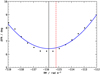 |
Fig. 1. Applying one RM to all the bursts detected during the observation of MJD 59243 and measuring the standard deviation of all the PA measurements from every time bin of every burst. Repeating this procedure for multiple RMs yields the black dots. The blue line is the fitted parabola. The vertical black line is the center of the fitted parabola. The red dashed vertical line is the RM measured after fitting using all the bursts. See Table 1 and Sect. 2.2. |
We illustrate the difference between the above approach of fitting one RM to all the bursts and inverse variance weighted average in Figure B.3. The top panel shows the difference of one RM fitted to all bursts (denoted with one) and the weighted average (denoted with wrm) for all MJDs. The bottom panel shows the significance of difference. A horizontal black dotted line is drawn at 3σ. The number in parenthesis next to MJDs is the number of bursts detected. The difference, although within 3σ, significantly changes the measured PA. In our observing band, from 550 MHz to 750 MHz, an RM offset of even one unit causes an offset in PA∞ by over 12 deg. Therefore, we only use one fitted RM for all the bursts to measure PAs. Moreover, we show the RM versus MJD using the measured RM, along with measurements from CHIME/FRB (Mckinven et al. 2023; Ng et al. 2025) and LOFAR (Gopinath et al. 2024) in Figure B.4.
Lastly, our choice of fitting one RM and one PA to all the bursts of an observation, which although works, has to be motivated from the data. To this end, we performed an experiment using all the bursts taken on the observation of MJD 59243, where we have over forty bursts. We apply one RM to all the calibrated bursts and measure the standard deviation of all the measured PAs from every time-sample of every burst. We repeat this procedure for different RMs. When we plot the standard deviation, denoted as ΔPA, against the applied RM, we get a parabola as shown in Figure 1 with black dots. The blue line shows the best fit parabola and the vertical black line is the center of the parabola. The vertical red dashed line is the fitted RM as described in the previous paragraph. With this, we note that one RM exists which reduces the spread in PAs, suggesting that fitting one RM and one PA to all the bursts of an observation is valid. Additionally, Figure B.5 shows by simulation, the spread in PA is only minimized if all the bursts indeed have the same RM and PA. If any one of either RM or PA is not the same, we do not recover any parabola, which further indicates that our attempt is valid.
2.3. Measuring PA
Having measured one RM and one PA for each observation, and having shown that one RM and one PA fits all the bursts within an observation, we bring the fitted PA from center frequency to infinite frequency using Eq. (1). The fitting, as mentioned before, is done with respect to center frequency of 650 MHz. At the same time, we apply the PA calibration correction as determined in Sect. 2.1 to compensate for PA offsets. The PA-calibrated, fitted PA at infinite frequency is denoted by ⟨PA∞⟩. The long-term analysis of FRB 20180916B is conducted with ⟨PA∞⟩. Alternatively, we can also extract using fitted RM and individual calibrated bursts. We apply the fitted RM to all the bursts of an observation using PAM, and extract PA and PA error time series using PDV The PA measured using PDV is with respect to the center frequency of the band, which can be easily brought to infinite frequency using Eq. (1). Thereafter, we compensate for PA offsets. The PA-calibrated, PA-measurements of individual bursts are denoted by PA∞.
The average of PA∞ is consistent with ⟨PA∞⟩, that is, the average of PSRCHIVE derived measurements is consistent with the fitted PA. Therefore, we only used ⟨PA∞⟩ as a measure of average. Instead of using the error in PA we get while fitting and propagating it, we use the standard deviation of PA∞ as a measure of error in ⟨PA∞⟩. The reason is as follows: the standard deviation of PA measurements from individual bursts would include the spread in PA due to DPHASE variations, intrinsic RM variations as we fit one RM to all the bursts and any intrinsic PA variations. For this same reason, we do not propagate the RM error into ΔPA, as that would have already been considered when taking standard deviation. Moreover, the fit error in PA is only of the order of 1 deg, which we think is heavily underestimated. We tabulate the ⟨PA∞⟩ and ΔPA measurements in Table 1. PA∞ measurements of each of the individual bursts are only presented in electronic form (see Data availability).
2.4. Credibility of measurements
We have had to use different calibration strategies using variety of different sources. The bursts of MJD 59243, 59244, 59274, 59275 and 59568 were calibrated using a single scan of 3C138 taken at the beginning of the observation. The bursts of MJD 59894, 59944, 60303, 60352 were calibrated using that noise diode scan that is nearest to when the burst occurred. The noise diode failed during the observation of MJD 59993. Therefore, the bursts of that observation were calibrated using the unpolarized quasar 3C48 and the PSR J0139+5814 pulsar following procedure described in SB24.
From the multiple noise diode scans taken within one observation but on different MJDs, in addition to the deviations from linear model of DPHASE (Figure A.3), we also observe variability in DPHASE data of one calibration scan to another (even with a separation of less than 30 minutes), although which is not significant enough to cause a change in linear DPHASE modeling and its linear parameters. Figure A.4 shows the variability as the difference between the DPHASE data of first scan and that of the consecutive scans for every observation. While we only noted the deviations and variations in DPHASE in the case of multiple noise diode scans, as DPHASE variations are a property of the observing instrument, we expect our calibration solutions constructed from quasars and pulsars to also suffer from the same issue. However, we reiterate that in spite of these variations, Dns and ψr parameters are consistent (Figure A.2) and do not show this variability reconfirming the validity of our calibration solutions.
In light of these instrumental deviations and variations of DPHASE, we investigate the impact this would have on our RM and PA measurements. Narrow band bursts show biases in RM measurements, as noted in Figure B.1. However, broad band bursts do not show those biases, as DPHASE deviations do not mimic Faraday rotation since they are not linear in λ2. We checked this by simulating bursts with known RM, PA and no structure, and superimposing the DPHASE deviations (as shown in Figure A.3) into simulated bursts’ PA as a function of frequency. Then, we recovered the true RM and PA, with differences in RM ≲ 0.2 rad m−2 and PA ≲ 0.4 deg, from all the simulated bursts which reaffirms us that broad band bursts are robust to DPHASE deviations. Having shown that broad band bursts are immune to DPHASE deviations, and since we fit for one RM and one PA using all the bursts of an observation, we are mimicking broad band bursts. To visualize this, we computed the cumulative distribution of the frequency spans of bursts detected within an observation in Figure B.6. The black bold line shows the cumulative uniform distribution over the frequency band. The collection of bursts from any observation occupies the whole band and thus behaves similar to a broad band burst and must be immune to DPHASE deviations. Therefore, we compare ⟨PA∞⟩ across observations, but since our fitting procedure does not take DPHASE deviations into account, which would manifest as colored noise when QU-fitting, there might be some bias. So, we err on the side of caution and only treat ⟨PA∞⟩ variability across observations at this point as preliminary. Accounting for the bias to robustly study the PA variability across observations will be taken up in a future work.
3. PA variability
We divided our discussion on PA variability in two parts: (i) intra-observation variability includes changes from burst to burst within a single observation (typically 2–4 hours) and (ii) inter-observation variability presents long-term changes on timescales ≥ day.
3.1. Intra-observation
In order to investigate burst-to-burst PA variations within an observation, we plot the PA∞ time series of every burst consecutively with different colors for different bursts in individual subplots for each observation in Figure 2. The PA∞ time series are rotated by -⟨PA∞⟩ from Table 1 so that they are all centered at 0. The gray shaded region is the 1σ error as presented in Table 1. Since PA∞ is plotted one after the other, there is no time-axis as such. It is simply concatenating PA∞ time series of bursts of an observation and plotting them with different colors. We note that PA∞ measurements are consistent with a single value even on the timescale of hours. This is also evident from the fact that we were able to fit all the bursts with a single PA and RM value (Sect. 2.2). That is, there is no sign of secular variability when the time separation between the bursts is of the order of hours (the “Sep” column in Table 1 provides the time separations). Since the maximum time separation in our dataset is about four hours (MJD 59243), we report an upper limit on variations of PA∞to be ≤7 deg within 4 hours (ΔPA of MJD 59243 from Table 1), and moreover, we note that this upper limit holds for all MJDs.
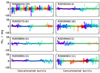 |
Fig. 2. PA∞ values of every time sample of each burst plotted one after the another in individual subplots for every MJD. Each PA∞ has been rotated by ⟨PA∞⟩ taken from Table 1. The different colors indicate different bursts. The shaded region around it is ΔPA, as reported in Tab. 1. The top left text in each subplot is the corresponding MJD and the number of bursts in parenthesis. |
3.2. Inter-observation
We start with a reminder that all inter observation PA variability is preliminary at this point. We first study the PA variability directly over MJD and over activity phase. PA variability could be tied with the periodicity of the FRB and must also be studied accordingly. The periodicity allows us to break time into an activity cycle and activity phase. PA can be independently varying over both activity phase and activity cycle. To disentangle both notions of variability, we followed the logic of studying PA variability by keeping either the activity phase or activity cycle constant and varying the other. Therefore, in the following subsections, we study the PA variations along three fronts: (i) the complete dataset versus MJD; (ii) the complete datasets, as well as measurements within a single activity cycle (intra-cycle), versus activity phase; and lastly (iii) measurements taken around the same activity phase (inter-cycle). In all the above-mentioned cases, ⟨PA∞⟩ measured across multiple observations are compared. Which, as already mentioned in Sect. 2.4, might possibly carry some bias. Therefore, we caution from overly interpreting the results at this point.
3.2.1. PA versus MJD
Figure 3 shows ⟨PA∞⟩ versus MJD. The colors indicate different activity cycles of the measurements, and the color-scheme used here is the same throughout the paper. We emphasize again here that we have corrected for long-term instrumental PA variation by aligning the PA swings of PSR B0329+54 and PSR J0139+5814 at different times (see Sect. 2.1 and Figure A.1). For FRB 20180916B, we observe a total spread in PA of about 80 deg over the ∼1100 days of monitoring, but ⟨PA∞⟩ versus MJD does not show clear evidence of a linear trend. However, we note that if there exists variability as a function of activity Phase and/or activity cycle, looking at PA against MJD may hide clear trends of this variability.
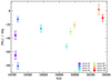 |
Fig. 3. ⟨PA∞⟩ versus MJD. The points are color coded according to their corresponding activity cycle. |
3.2.2. PA versus phase
We plot ⟨PA∞⟩ and PA∞ versus activity phase in Figure 4 as markers with black border and faint markers respectively. We note that to avoid PA wrap arounds, we have rotated PA∞ and ⟨PA∞⟩ by 45 deg. The range of ⟨PA∞⟩ measurements in both the datasets is around 80 deg. Although, we have 10 measurements, they occur only at five distinct activity phases.
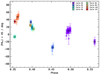 |
Fig. 4. ⟨PA∞⟩ versus activity phase of FRB 20180916B plotted with markers with a black border. PA∞ versus activity phase of the bursts plotted with faint markers. Both PA∞ and ⟨PA∞⟩ have been rotated by 45 deg. |
We have two instances with more than one measurement from the same activity cycle (see Table 1). Two observations were made in (i) Cycle-53 on MJD 59243 and 59244 and (ii) Cycle-55 on MJD 59274 and 59275. Cycle-53 observation pair phase ranges from 0.494 to 0.562 (26.52 hours), whereas Cycle-55 observation pair ranges from 0.397 to 0.453 (22.13 hours). We study the variability within the same activity cycle, which we call intra-cycle variability, using the rate of change of PA. In Cycles 53 and 55, the rates of change of PA computes to be −58.8 and −29.2 deg activity phase−1 respectively, or in regular units, −1.0 and −3.2 deg h−1 respectively or For both the pairs, the significance of variability is at least 3σ. Interestingly, we note that rates of change of PA is different for these two pairs, which suggests rate of intra-cycle variability depends on activity phase.
We test if intra-cycle variability is consistent with the observed non-variability of PA∞≤7 deg over four hours of observation of MJD 59243 (activity cycle 53, see Sect. 3.1 for details). With the intra-cycle variability slope of −1.0 deg h−1 from Cycle-53, in a span of four hours, we expect to see variations of around 4 deg. The ΔPA of MJD 59243 observation (whose session was four hours in duration) is 6.27 deg, which means observed intra-cycle variation is consistent at 1.5σ with our non-variability of PA observation. This suggests that PA is varying against activity phase slowly enough that on timescales of four hours or less, the PA appears to be constant.
3.2.3. Inter-cycle at a constant phase
Two of the five clusters in activity phase have more than one ⟨PA∞⟩ measurement. ⟨PA∞⟩ measurements of MJD 59894, 60303, and 60352 are within a phase separation of 0.008 (three hours), with a mean phase of 0.359. We denote this cluster by G1. Also, ⟨PA∞⟩ measurements of MJD 59274, 59568, 59944 and 59993 all are within a maximum phase separation of 0.006 (2.75 hours) and a mean phase of 0.400, which we denote by G2. We plot the ⟨PA∞⟩ versus activity cycle for both the clusters in Figure 5 in blue and red respectively. The top x-axis is in MJD since the reference MJD of the periodicity model of FRB 20180916B. The ⟨PA∞⟩ measurements where we only have one burst are shown with black markers. We find that for both the clusters there is a clear sign of variability. That is, ⟨PA∞⟩ measurements taken at the same activity phase varies against activity cycle. While we do not see a clear trend, if we ignore the ⟨PA∞⟩ measurements with only one burst (shown with black markers), we still notice variability. Therefore, we report inter-cycle variability and wait until more ⟨PA∞⟩ measurements are made at similar activity phases to further characterize it.
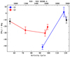 |
Fig. 5. ⟨PA∞⟩ versus activity cycle for the two phase clusters: G1 and G2. G1 refers to the ⟨PA∞⟩ measurements made at around Phase 0.359 (MJD 59894, 60303 and 60352) and G2 at around Phase 0.400 (MJD 59274, 59568, 59944, 59993). See Sect. 3.2. The black markers are used to denote those ⟨PA∞⟩ measurements with only one burst. The top x-axis shows MJD of the ⟨PA∞⟩ measurements. We emphasize that the reference MJD of the top x-axis is that of the periodicity model of FRB 20180916B. |
Simply, as an order of magnitude estimate, we can compute the rates of change from the two clusters. The rates of change is around ∼0.1 deg day−1 For comparison, when studying ⟨PA∞⟩ versus MJD, we noted 80 deg change over 1100 days, which amounts to a rate of change of 0.07 deg day−1 which is partly consistent with what we measure here. The inter-cycle variability is of the order of deg day−1, whereas the intra-cycle variability is of the order of deg h−1, which suggests there are two scales of variability. Having said so, we do not have sufficient measurements to fully study the inter-cycle variability. It could be simply PA variability linear in time which does not follow the periodicity of the source. At this point, we cannot comment further. We again remind that we have performed PA calibration and have performed PA-calibration, that is accounted for any inter-observation PA offsets using PA-sweeps of pulsars (Sect. 2.1 and Figure A.1).
4. Constraints on progenitor models
In this section we connect the observed PA variability in conjunction with the periodicity of the FRB 20180916B, to what is predicted by various progenitor models and place constraints on the geometry of the models. We only focus on neutron star progenitor models, that is, where bursts originate from the magnetosphere of the neutron stars. Since they originate from the magnetosphere, the PA of the bursts carry the information about the dynamics of the neutron stars. Specifically, we test various progenitor models against the following observations:
Since, we are treating all inter observation PA variability results as preliminary, we nevertheless discuss them in terms of models, but refrain from ruling out any model solely based on them at the moment (also see Sect. 2.4).
4.1. Slow rotation
In a slowly rotating neutron star model for FRB 20180916B, the rotational period is the period of the FRB (16.34 days; Beniamini et al. 2020; Li & Zanazzi 2021). It is analogous to a typical pulsar except that the period is extremely large. We understand the geometry the following way: an inertial frame is attached to the center of the neutron star such that the rotation axis is along the Z-axis (toward up), X-axis is toward right, and the observer is located somewhere in the XZ-plane. We suppose that burst emission is directed along an arbitrary axis co-rotating with the neutron star, which we call the emission axis. We illustrate the geometry in Figure 6 (left). The PA is the angle between the planes formed by observer and rotation axis, and observer and emission axis. It is illustrated in the same figure. Moreover, the burst emission has the same PA along the emission axis at all times. In case of pulsars, this emission axis is the dipolar magnetic axis and the emission mechanism is curvature radiation (Mitra et al. 2024). As the neutron star rotates, the projection of the emission axis on the sky changes. This change in projection of the emission axis is tracked by the PA of the observed emission. We note that this change in PA is not caused by the emission mechanism, but due to the rotation motion, hence is dynamical and geometrical in nature. The projection is modeled with RVM (Everett & Weisberg 2001):
 (2)
(2)
Here, α and ϕ0 are the magnetic axis co-latitude and longitude in the inertial frame respectively. ζ is the co-latitude of the observer, which is also known as viewing angle and PA0 is the projection of the spin-vector in the sky. The magnetic field need not just be dipolar; axis-symmetric multi-pole magnetic fields also follow RVM (Qiu et al. 2023). Therefore, our testing is still valid even if our assumption of dipolar magnetic field does not hold. However, the same cannot be said for general multi-pole magnetic fields.
In this model, since the period is large, the PA shows a slow rate of change, which satisfies O1. In addition, we expect intra-cycle PA variations, which satisfies O2. Modeling of the intra-cycle PA variations with more measurements would help further constrain this model. If the intra-cycle PA variations are RVM-like, the magnetic field configuration would be dipole-like. However, in any case, there would be no variations in PA across the activity cycle at the same activity phase, contrary to O3. In other words, according to this model, all the variations seen in G1 and G2 are random. This would be equivalent to the random variations in PAs of individual pulses of pulsars compared to that of the integrated pulse at the same phase (See Figure 2 Johnston et al. 2024). (Also see Figure 1 of Mitra et al. (2007) where the PA values show scatter about the RVM curve.) Lastly, we observed the range of ⟨PA∞⟩ measurements span across 80 deg. Within the RVM model, the range of PA values is decided by α. A larger α leads to a larger range of PA values. However, with ⟨PA∞⟩ measurements at only five distinct activity phases, any RVM modeling or constraining α would not be robust. Therefore, we defer actual RVM fitting to future work.
4.2. Fast precession
In the fast precession model for FRB 20180916B, the burst emitting neutron star is rotating with a spin period and is also freely precessing with a precessional period (Zanazzi & Lai 2020; Li & Zanazzi 2021). Free precession implies there are no resultant torques on the compact object, which implies, the angular momentum is a constant of motion. The precessional period is assumed to be the activity period of the FRB (16.34 days), and the spin period is predicted to be of the order of seconds (Levin et al. 2020; Zanazzi & Lai 2020). Our geometry for precession is identical to that presented in Li & Zanazzi (2021). The geometry of this case is described as follows: Instead of inertial frame, we attach a body fixed frame at the center of the neutron star such that the precession axis (or the symmetric axis, the axis along which the body is symmetric) is along Z-axis and the emission region (which is fixed in body fixed frame) is in XZ-plane. The rotation axis is at a separation of δ (θ in Jones & Andersson 2001). We make a reasonable assumption that rotation dominates the angular momentum, thereby, the separation between the rotation axis and angular momentum axis ( in Jones & Andersson 2001) is extremely small, and is of the order of the square of the deformity of the neutron star. Then, PA is defined as the angle between the planes formed by observer and rotation axis, and observer and emission axis. Because of our assumption, this PA definition is with respect to a constant reference axis (like angular momentum axis). δ is treated as a free parameter, which is known as the wobble angle (Jones & Andersson 2001). We provide a cartoon illustration in Figure 6 (right). The observer in the body fixed frame executes the precession dynamics, which can be understood as the observer rotating about the rotation axis with rotational period and the rotation axis rotating about the precession axis with precessional period. If we define the observer to be at ζ separation from rotation axis (like in Sect. 4.1), we note that co-latitude of observer as seen in the body fixed frame changes from |ζ − δ| to ζ + δ within a rotational period. This co-latitude variability happens for every rotational period at every precessional phase. Ultimately, it causes PA variations over the rotational period timescales.
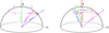 |
Fig. 6. Illustration of rotation (left) and precession (right) geometries considered here. The left image is shown in the inertial coordinate system, which is fixed at the center of the neutron star. The right image is shown in the body fixed coordinate system. The X-axis is toward the right. The Z-axis is up. In case of rotation (left), the rotation axis is along Z-axis. In case of precession (right), the precession axis (symmetric axis) is along Z-axis. Motion is illustrated with large dashed line having arrows at regular intervals. The measured PA is appropriately marked. |
We observed that PA is ≤7 deg on timescale of at least four hours (O1) for multiple observations. If the emission region was such that it only partially overlapped with the trajectory of observer, we would have been able to recover the periodicity. Since no short timescale periodicity has been found in FRB 20180916B, we suggest that the emission region is large enough to not cause any periodicity signature. We also know that the modulation of PA values constrains α, which gives us the constraint α ≪ ζ. The maximum range of α is |δ + θ|, and therefore, |δ + θ|≪ζ. If the variability of PA is constrained to be ≤7 deg (O1), both δ and θ ≲ 10 deg, which causes ζ ≳ 30 deg. In words, the rotation axis and emission axis are in close proximity to the precession axis, but the observer is far away from the rotation axis.
Firstly, such a configuration cannot produce a modulation of 80 deg of ⟨PA∞⟩ over activity phase (Figure 4). In addition, a fast precession model also cannot explain inter cycle variation (O3). The geometry of the entire system at any activity phase is identical for all activity cycles, which implies the observed PAs cannot be different for different activity cycles at the same activity phase. The above inter-observation PA variability results directly make fast precession extremely unlikely. Regardless, even by only relying on intra-observation PA non-variability result (O1), we can concretely rule out fast precession model. With the above-mentioned geometric constraint from O1, it is almost impossible to provide an emission region which is large enough to cover all the spin-phases but which can only provide 30% duty cycle in activity period.
4.3. Slow precession
The slow precession model for FRB 20180916B is similar to the fast precession model, except that the spin period is the activity period of the FRB (that is, 16.34 days) and the precessional period is much longer than the activity period. Therefore, this model is the equivalent to a combination of slow rotation, which explains non-variability and intra-cycle variability (O1 and O2), and free precession, invoked to explain inter-cycle variability (O3). However, precession would cause a gradual change in the active window that has not been seen, which implies this model cannot directly explain the periodicity.
An alternate test for this model would be to study the inter-cycle variability. If that variability is indeed caused by precession, PAs at the same activity phase would exhibit sinusoidal variations with a period given by the precessional period, and the range of variation would be of the order of δ (defined in Sect. 4.2). We provide a simulation of this effect in Appendix C. We cannot yet estimate the precession period. However, a lower limit of the precessional period would be the maximum time span of activity phase clusters – G1 and G2, as we do not observe a full period yet, which is around 800 days. Now, if we assume an ellipticity of 10−4 (Levin et al. 2020) or 10−6 − 10−8 (Desvignes et al. 2024), and a rotational period of 16.34 days, the precessional period is  days. Even if we take the smallest precessional period of ∼105 days, a maximum time span of 800 days would only mean a precessional phase span of 3 deg. For us to observe at least 50 deg of ⟨PA∞⟩ variation within the 3 deg precessional phase span suggests an extremely large sinusoidal amplitude or δ, which is highly unlikely. Therefore, we conclude that maximum precessional period would be much less than ∼105 days. We defer the attempt to accurately measure precessional period until inter cycle variability is measured with more significance and its variability is characterized.
4.4. Binary models
There are various binary models proposed to explain the periodicity and chromaticity of FRB 20180916B, but in this work, we only focus on such models where one of the bodies is a burst emitting compact object (Ioka & Zhang 2020; Wada et al. 2021; Li et al. 2021). For instance, in Ioka & Zhang (2020) and Wada et al. (2021), the emitting object is a neutron star, while in Li et al. (2021) the central object is a Be-type star with a disk and the bursts arrive from a compact object orbiting the star. In all cases, the period of the binary orbit is assumed to be the activity period of the FRB (16.34 days).
Whether or not PAs carry any information about the binary motion depends on whether there is coupling between the emitting object’s angular momentum and the system’s orbital angular momentum (Hamilton & Sarazin 1982). In point mass Keplerian dynamics, there is no such coupling. The orientations of the objects are not governed by their binary motion. If PAs track the instantaneous orientation of the object, such PAs would not carry any information about the binary motion and thus could not be used to probe binary models. However, if we assume a binary model scenario where the PA of the emitted burst is purely a function of the true anomaly of the burst emitting object, we can perform some model testing. As the orbital period is the same as the activity period, the predicted intra-cycle PA variability will match the observed variability. Then to explain inter cycle variability, we would need to invoke some form of binary precession. Modeling and testing such scenarios is a work in itself and requires much more measurements for any meaningful test. Hence, it will be taken up in future work.
That said, there are PA models for relativistic spin precession (Kramer & Wex 2009), which have been used for Double Neutron Star systems such as PSR J1906+0746 (Desvignes et al. 2019) and PSR J1946+2052 (Meng et al. 2024). In this case, we suppose the orbital period to be activity Period of the FRB. The lack of any PA variations over rotational period timescales constrains α, just like in the case of Fast precession (Sect. 4.2). In addition, due to relativistic spin precession, the projection of the spin vector (Ψ0) changes all the time throughout the orbit on spin-precession timescale (Eq. 6; Meng et al. 2024). That is, Ψ0 is periodic with precessional period and does not depend on orbital phase (which is activity phase in this case). However, we do not see any such signature in ⟨PA∞⟩ versus MJD (Sect. 3.2.1) and we know there are two scales of variability – intra-cycle and inter cycle are tied with the periodicity of the FRB (orbital period). Therefore, we do not suppose a relativistic spin precession model can explain the observed PA variations.
5. Discussions
5.1. APERTIF PA sample
Pastor-Marazuela et al. (2021) measured PAs from the bursts detected using APERTIF at 1370 MHz at different activity phases and cycles. They report a range of PA values of around 44 deg over a phase span of 0.1 (1.5 days), while we report a range of ⟨PA∞⟩ values of around 80 deg (Figure 4 and Sect. 3.2.2) and a phase span of 0.2 (3.25 days). Moreover, Pastor-Marazuela et al. (2021) have multiple PA measurements within Cycle-37 and -38, which we use here to test intra-cycle variability. We plot the PA measurements of Cycle-37 (in red) and Cycle-38 (in blue) against activity phase in Figure 7. We connect those measurements which are done in the same observing session with a line. Moreover, we add vertical dotted lines at intervals of 4 hours starting from the smallest phase.
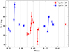 |
Fig. 7. Position angle measurements of bursts detected by APERTIF at 1370 MHz in activity cycle-37 and -38 (Pastor-Marazuela et al. 2021). Line connecting squares denotes measurements taken in the same observing session. The black dotted line is drawn for every four hours of phase-separation. |
Unlike in our analysis, Pastor-Marazuela et al. (2021) used a singular RM value for all the bursts, which were detected across multiple observations and cycles, and in addition, the bursts have been absolutely calibrated, i.e., PAs can be studied across Phase and Cycle. While we observe PA variability < 7 deg over four hour timescale, Pastor-Marazuela et al. (2021) observes much rapid variability on these timescales. Furthermore, PAs measured from bursts within the same observing epoch also exhibit large variability, contrary to what we report. We cannot test inter cycle variability as the Pastor-Marazuela et al. (2021) dataset does not multiple measurements at the same activity phase.
This inconsistency can be explained in the following way. The PA measurements of Pastor-Marazuela et al. (2021) have been made after correcting all the bursts with the same RM of −115 rad m−2. All the measurements were made when the RM was only stochastically varying (Mckinven et al. 2023). The standard deviation of the RM measurements in the stochastic regime (before MJD 59200) is about 3 rad m−2 (Mckinven et al. 2023). PA measurements are at frequency of 1370 MHz, which even for a RM variability of the order of 3 rad m−2 causes a PA variability of about 8 deg. Therefore, the observed variability by Pastor-Marazuela et al. (2021) could be due to the use of a single RM for all observations rather than observation-specific RMs as used in this analysis.
5.2. Her X-1
Her X-1 is an intermediate mass accreting X-ray binary pulsar system in which the neutron star spins with a period of 1.24 seconds, the orbital period is 1.70 days and the whole system also shows a superorbital period of 35 days. The super-orbital period in Her X-1 has been attributed to a precessing accretions disk (see, e.g., Katz 1973). In recent work by Heyl et al. (2024), neutron star’s polarization profile was modeled with RVM at different times, through which the superorbital periodicity is explained using complex rotational dynamics involving rotation and precession of the neutron star, accretion disk and the companion. The activity of Her X-1 switches states of activity multiple times over the superorbital periodicity (Scott et al. 2000). It has two ON-states known in literature as main-on and short-on. According to Heyl et al. (2024), the activity variability of Her X-1 is caused by the crustal precession, which brings the active emission region into the line of sight of the observer at specific precessional phase. The extent of active region along the line of sight determines the scale and length of activity seen. We can immediately draw many parallels between Her X-1 and FRB 20180916B. Firstly, the rate variability over superorbital period is analogous to rate variability seen over active window (Pastor-Marazuela et al. 2021, SB24). Moreover, if the observer sees different emission regions at different phases, and if such emission regions emit at different frequencies, we could directly also explain chromaticity (c.f. Li & Zanazzi 2021).
The superorbital periodicity of Her X-1 is known to be stable (Staubert et al. 2009). If the cause of that periodicity is indeed precession, one would assume various damping mechanisms to be at play, which would lengthen the period with time (Katz 2021). However, Heyl et al. (2024) show how torque interactions between disk and the star balance out the opposing torques such that the resultant motion is effectively torque free. Now compare with FRB 20180916B for which Sand et al. (2023) and Lan et al. (2024) report that the period of FRB 20180916B is stable over at least two years.
Heyl et al. (2024) notes a change of about 8 deg in the Ψ0 between two main-on states, which are separated by over an year (Table 1, χp column of Heyl et al. 2024). The PA variability gives a slope of 0.02 deg day−1. This is largely consistent with the inter-cycle variability slopes we measure in Sect. 3.2. Heyl et al. (2024) suggest that this variability is caused by a change in the angular momentum. While it is unclear at the moment what could be causing the angular momentum changes, we note that in free-precession regime the angular momentum is a constant of motion, as there are no torques involved. As noted in the previous paragraph, even if there are multiple torques at play and if all the torques balance out, the resulting system can maintain its period and also change its angular momentum.
Her X-1 is observed in optical and X-rays, with only a marginal detection in radio at 9 GHz(van den Eijnden et al. 2018). If FRB 20180916B is a source similar to Her X-1, we should expect to see temporal variability of optical and X-ray light curves over rotational and/or binary period timescales. This temporal variability should be persistent irrespective of the state of FRB 20180916B in radio. However, no such optical or X-ray emission is detected. One reason could be the burst emission is beamed elsewhere. Although more likely, it could be due to large distance of FRB 20180916B (140 Mpc) compared with that of Her X-1 (7 kpc). If we assume a X-ray luminosity of ∼1037 erg s−1 for Her X-1(Brecher 1972), and if we place Her X-1-like source at the distance of FRB 20180916B, the observed X-ray luminosity is ten times less than the upper limit provided by Swift-BAT (Laha et al. 2022). Which suggests that large distance is hindering any X-ray detection. And if Her X-1 (or other such systems that exhibit superorbital periodicity, see Kotze & Charles 2012) are similar to FRB-sources, we should expect to detect FRB-like bursts. In so far, no such bursts have been detected, which could suppose that comparison is not so direct.
5.3. Other repeating FRBs
The current population of known repeating FRBs shows a diversity of PPA behavior within single bursts, as well as between bursts within a single observation. (We reiterate that this is the first robust study of PPA variation between different observations.) FRB 20121102A also exhibits flat PPA curves within individual bursts (Hilmarsson et al. 2021), and notably, bursts within a single observation can also be fit with a single RM and PPA value (Michilli et al. 2018). A small sample of bursts from FRB 20200120E show flat PPAs across a burst but jumps in the PPA value from burst-to-burst (Nimmo et al. 2022). This is in contrast to FRB 20180301A, FRB 20201124A, FRB 2022012A, which show swings in PAs across the duration for some bursts and burst-to-burst variations within an observation (e.g., Luo et al. 2020; Jiang et al. 2022; Zhang et al. 2023). That said, there is evidence that some of this may due to propagation effects through the plasma (Uttarkar et al. 2024; Xu et al. 2022), which complicates the connection between the PPA and the geometry at the emission site.
FRB 20180916B’s PPA properties are most similar to FRB 20121102A. Interestingly FRB 20121102A is also the only other repeating FRB with a known activity periodicity (Rajwade et al. 2020; Braga et al. 2025). With a sample size of two, it is difficult to judge whether this is simply a coincidence. Moreover, the host galaxies and local environments of the two sources are different. FRB 20180916B is on the edge of a star forming region within a spiral galaxy and has no associated PRS (Marcote et al. 2020), while FRB 20121102A is in a star forming region in a low metallically dwarf galaxy and has a PRS (Marcote et al. 2017; Tendulkar et al. 2017). If they have the same progenitor, it needs to be able to be present in both these environments.
5.4. Future strategies
Future observing campaigns should focus on studying intra-cycle variability and robustly investigating inter cycle variability. Studying intra-cycle variability requires repeated observations of the source within the same activity cycle for multiple cycles. Investigating inter cycle variability would require us to perform observations at the same activity phase on many different activity cycles. Therefore, in addition to being able to track the source over long times, we would also need a sufficient burst rate to robustly measure the RM and track the PA variability. Given these requirements, we argue that the uGMRT is the first choice for this endeavor. uGMRT can observe the source for around 11 hours continuously on average, which means it would require over ten days to cover the entire 5.1 days active window at 600 MHz. In addition, uGMRT at 650 MHz observes a rate of well over one per hour (SB24).
Performing a long-term PA variability study requires a stable PA reference frame so that we do not introduce any PA offsets. In this study, we test for this stability by using multiple pulsar observations taken on four different epochs. We find agreement between the PA offset found using each of the pulsar PA sweeps when compared to the respective PA reference sweep (see Table A.1). This agreement should be valid throughout the span of the study. Considering that the reference PA frame used here is non-standard, it would be worthwhile to connect the reference PA frame with absolute reference frames such as those defined in Perley & Butler (2013). Such a connection would also be useful as an independent probe of PA validity.
We have to improve our calibration strategy. From this study, we find that deviations from our linear model of DPHASE exist and impact our RM measurements. Therefore, sophisticated calibration strategies could first be developed. Alternatively, we can improve our fitting strategy to include Gaussian Processes that can can account for DPHASE variations to measure unbiased RM and PA estimates. In addition, our procedure of fitting one RM and PA to all the bursts is althought robust, it requires a sufficient number of bursts to perform as expected. Future observing strategies could take that into account and observe the source for sufficiently long duration. All in all, this work seeks to prompt many future work in this direction, and in particular, study such PA variations of other repeating FRBs. Of all the known repeating FRBs, in particular, we want to highlight FRB 20200120E which has been localized to a globular cluster (Kirsten et al. 2022). The properties of the bursts strongly suggest that young pulsar progenitor model produces bursts (Nimmo et al. 2022). If that is the case, PAs of the bursts would already carry an RVM-like signature, which can provide further evidence.
6. Conclusions
We have presented consistent, almost absolute calibrated PA measurements of 84 bursts of FRB 20180916B collected over a time span of 1200 days with the uGMRT at 650 MHz. We have performed a PA calibration (Sect. 2.1 and Figure A.1), showed and fit one RM and one PA to all the bursts from an observation (Sect. 2.2), and measured observation averaged PA and its error from all the observations (Sect. 2.3).
We suggest that PA variability is best understood when studied in conjunction with the periodicity of the FRB. While we report the following findings, we note that possible biases in ⟨PA∞⟩ make comparison with ⟨PA∞⟩ across different observations only preliminary at this point (Sect. 2.4):
-
The variability in PA is constrained to be ≤7 deg over timescales of four hours (O1) in all observations.
-
The PA varies over activity phase, which we referred to as intra-cycle variability, with a variability of ∼ ± 1 h−1 (O2) or 80 deg over 0.2 Phase units.
-
We also report that the PA varies with activity cycle, which we have studied by using ⟨PA∞⟩ measured at the similar activity phases. We call this variability inter-cycle variability, which is of the order of 0.1 deg day−1 (O3).
We are able to place constraints on various dynamical models for the FRB using the above-mentioned findings. Given that our inter-observation PA variability is only preliminary, we tested the models based on O2 and O3 but do not rule out any solely based on them.
-
A slowly rotating model due to the large rotational period can explain the limited variability over timescales of hours and intra-cycle variability (O1 and O2). We conclude that a slowly rotating model can explain FRB 20180916B. However, such a model cannot explain inter-cycle variability (O3) without suggesting the observed inter-cycle variability is purely caused by random variations.
-
Fast precession models predict rotational-timescale PA variability, which is at odds with the non-variability of PA on timescales of hours (O1). Moreover, satisfying O1 causes the model to contradict the following observations: (i) a lack of any short timescale periodicity, (ii) a 30% duty cycle of the active window, and (iii) observed PA versus activity phase modulation (O2). In addition, a fast precession model cannot explain O3. Therefore, at this point, we successfully rule out the fast precession model.
-
The slow precession model is equivalent to the combination of slow rotation and free precession, which can explain O1, O2, and O3. However, under this model, the active window should change with time, which has not been observed. Notwithstanding, this model predicts sinusoidal inter-cycle PA variations that can also be used to test this model with future measurements.
-
Testing binary models, where the binary orbital period causes the periodicity of the source, requires models to make PA predictions, which as of now, none of the proposed models do. Testing such models will be done in a future work. Nevertheless, if we suppose FRB 20180916B is similar to a double neutron star system exhibiting relativistic spin precession (Kramer & Wex 2009), O1 can constrain the RVM geometry. However, ⟨PA∞⟩ variations would not follow the periodicity of the FRB, which contradicts O2 and O3.
Lastly, we compared FRB 20180916B with the Her X-1 system and highlighted many similarities in Sect. 5.2. The most insightful of them all is the consistency between the rate of PA variability of Her X-1 measured in the X-ray using IXPE (Heyl et al. 2024) and the inter-cycle variability of FRB 20180916B measured in the radio using uGMRT. Continuing the long-term study of PAs of both the systems can possibly provide new avenues to compare and understand both objects.
Data availability
All the burst averaged PA∞ measurements are available at the CDS via https://cdsarc.cds.unistra.fr/viz-bin/cat/J/A+A/702/A248. Any other data from this article will be shared on any request to the corresponding author.
When light of frequency f propagates through a distance of L, it acquires a phase (ϕ) of  . Then, the difference in phase (Δϕ) due to different propagation lengths (ΔL) is
  . If ΔL is a constant of f, Δϕ is a linear function of f.
Acknowledgments
SB is grateful to Gregory Desvignes for his attention to detail, his comments on this work, and most importantly his patience, all of which greatly improved the quality of the paper. SB also extends his gratitude to the reviewer for their comments. We thank the staff of the GMRT that made these observations possible. GMRT is run by the National Centre for Radio Astrophysics of the Tata Institute of Fundamental Research. VRM gratefully acknowledges the Department of Atomic Energy, Government of India, for its assistance under project No. 12-R&D-TFR-5.02-0700. LGS is a Lise Meitner Independent Max Planck research group leader and acknowledges support from the Max Planck Society.
References
- Bailes, M. 2022, Science, 378, abj3043 [NASA ADS] [CrossRef] [Google Scholar]
- Beniamini, P., Wadiasingh, Z., & Metzger, B. D. 2020, MNRAS, 496, 3390 [NASA ADS] [CrossRef] [Google Scholar]
- Bera, A., James, C. W., Deller, A. T., et al. 2024, ApJ, 969, L29 [Google Scholar]
- Bera, A., James, C. W., McKinnon, M. M., et al. 2025, ApJ, 982, 119 [Google Scholar]
- Bethapudi, S., Spitler, L. G., Main, R. A., Li, D. Z., & Wharton, R. S. 2023, MNRAS, 524, 3303 [NASA ADS] [CrossRef] [Google Scholar]
- Bethapudi, S., Spitler, L. G., Li, D. Z., et al. 2025, A&A, 694, A75 [NASA ADS] [CrossRef] [EDP Sciences] [Google Scholar]
- Braga, C. A., Cruces, M., Cassanelli, T., et al. 2025, A&A, 693, A40 [NASA ADS] [CrossRef] [EDP Sciences] [Google Scholar]
- Brecher, K. 1972, Nature, 239, 325 [Google Scholar]
- Britton, M. C. 2000, ApJ, 532, 1240 [CrossRef] [Google Scholar]
- CHIME/FRB Collaboration (Andersen, B. C., et al.) 2019, ApJ, 885, L24 [Google Scholar]
- Chime/Frb Collaboration (Amiri, M., et al.) 2020, Nature, 582, 351 [NASA ADS] [CrossRef] [Google Scholar]
- Desvignes, G., Kramer, M., Lee, K., et al. 2019, Science, 365, 1013 [Google Scholar]
- Desvignes, G., Weltevrede, P., Gao, Y., et al. 2024, Nat. Astron., 8, 617 [Google Scholar]
- Everett, J. E., & Weisberg, J. M. 2001, ApJ, 553, 341 [NASA ADS] [CrossRef] [Google Scholar]
- Gopinath, A., Bassa, C. G., Pleunis, Z., et al. 2024, MNRAS, 527, 9872 [Google Scholar]
- Gupta, Y., Ajithkumar, B., Kale, H. S., et al. 2017, Curr. Sci., 113, 707 [NASA ADS] [CrossRef] [Google Scholar]
- Hamilton, A. J. S., & Sarazin, G. L. 1982, MNRAS, 198, 59 [Google Scholar]
- Heyl, J., Doroshenko, V., González-Caniulef, D., et al. 2024, Nat. Astron., 8, 1047 [NASA ADS] [CrossRef] [Google Scholar]
- Hilmarsson, G. H., Michilli, D., Spitler, L. G., et al. 2021, ApJ, 908, L10 [NASA ADS] [CrossRef] [Google Scholar]
- Hotan, A. W., van Straten, W., & Manchester, R. N. 2004, PASA, 21, 302 [Google Scholar]
- Ioka, K., & Zhang, B. 2020, ApJ, 893, L26 [NASA ADS] [CrossRef] [Google Scholar]
- Jiang, J.-C., Wang, W.-Y., Xu, H., et al. 2022, Res. Astron. Astrophys., 22, 124003 [CrossRef] [Google Scholar]
- Johnston, S., Karastergiou, A., Keith, M. J., et al. 2020, MNRAS, 493, 3608 [NASA ADS] [CrossRef] [Google Scholar]
- Johnston, S., Kramer, M., Karastergiou, A., et al. 2023, MNRAS, 520, 4801 [Google Scholar]
- Johnston, S., Mitra, D., Keith, M. J., Oswald, L. S., & Karastergiou, A. 2024, MNRAS, 530, 4839 [Google Scholar]
- Jones, D. I., & Andersson, N. 2001, MNRAS, 324, 811 [Google Scholar]
- Kaspi, V. M., & Beloborodov, A. M. 2017, ARA&A, 55, 261 [Google Scholar]
- Katz, J. I. 1973, Nat. Phys. Sci., 246, 87 [Google Scholar]
- Katz, J. I. 2021, MNRAS, 502, 4664 [CrossRef] [Google Scholar]
- Kirsten, F., Marcote, B., Nimmo, K., et al. 2022, Nature, 602, 585 [NASA ADS] [CrossRef] [Google Scholar]
- Kotze, M. M., & Charles, P. A. 2012, MNRAS, 420, 1575 [NASA ADS] [CrossRef] [Google Scholar]
- Kramer, M., & Wex, N. 2009, Class. Quant. Grav., 26, 073001 [Google Scholar]
- Laha, S., Wadiasingh, Z., Parsotan, T., et al. 2022, ApJ, 929, 173 [Google Scholar]
- Lan, H.-T., Zhao, Z.-Y., Wei, Y.-J., & Wang, F.-Y. 2024, ApJ, 967, L44 [Google Scholar]
- Landau, L. D., & Lifshitz, E. M. 1976, Mechanics, Third Edition: Volume 1 (Course of Theoretical Physics), 3rd edn. (Butterworth-Heinemann) [Google Scholar]
- Levin, Y., Beloborodov, A. M., & Bransgrove, A. 2020, ApJ, 895, L30 [NASA ADS] [CrossRef] [Google Scholar]
- Li, D., & Zanazzi, J. J. 2021, ApJ, 909, L25 [Google Scholar]
- Li, Q.-C., Yang, Y.-P., Wang, F. Y., et al. 2021, ApJ, 918, L5 [NASA ADS] [CrossRef] [Google Scholar]
- Lorimer, D. R., & Kramer, M. 2012, Handbook of Pulsar Astronomy (Cambridge, UK: Cambridge University Press) [Google Scholar]
- Lorimer, D. R., Bailes, M., McLaughlin, M. A., Narkevic, D. J., & Crawford, F. 2007, Science, 318, 777 [Google Scholar]
- Luo, R., Wang, B. J., Men, Y. P., et al. 2020, Nature, 586, 693 [NASA ADS] [CrossRef] [Google Scholar]
- Marcote, B., Paragi, Z., Hessels, J. W. T., et al. 2017, ApJ, 834, L8 [CrossRef] [Google Scholar]
- Marcote, B., Nimmo, K., Hessels, J. W. T., et al. 2020, Nature, 577, 190 [NASA ADS] [CrossRef] [Google Scholar]
- Mckinven, R., Gaensler, B. M., Michilli, D., et al. 2023, ApJ, 950, 12 [NASA ADS] [CrossRef] [Google Scholar]
- Mckinven, R., Bhardwaj, M., Eftekhari, T., et al. 2024, arXiv e-prints [arXiv:2402.09304] [Google Scholar]
- Meng, L., Zhu, W., Kramer, M., et al. 2024, ApJ, 966, 46 [Google Scholar]
- Michilli, D., Seymour, A., Hessels, J. W. T., et al. 2018, Nature, 553, 182 [Google Scholar]
- Mitra, D., Rankin, J. M., & Gupta, Y. 2007, MNRAS, 379, 932 [NASA ADS] [CrossRef] [Google Scholar]
- Mitra, D., Basu, R., & Melikizde, G. I. 2024, Universe, 10, 248 [Google Scholar]
- Ng, C., Pandhi, A., Mckinven, R., et al. 2025, ApJ, 982, 154 [Google Scholar]
- Nimmo, K., Hessels, J. W. T., Keimpema, A., et al. 2021, Nat. Astron., 5, 594 [NASA ADS] [CrossRef] [Google Scholar]
- Nimmo, K., Hessels, J. W. T., Kirsten, F., et al. 2022, Nat. Astron., 6, 393 [NASA ADS] [CrossRef] [Google Scholar]
- Pastor-Marazuela, I., Connor, L., van Leeuwen, J., et al. 2021, Nature, 596, 505 [NASA ADS] [CrossRef] [Google Scholar]
- Perley, R. A., & Butler, B. J. 2013, ApJS, 206, 16 [Google Scholar]
- Petroff, E., Hessels, J. W. T., & Lorimer, D. R. 2019, A&A Rev., 27, 4 [NASA ADS] [CrossRef] [Google Scholar]
- Petroff, E., Hessels, J. W. T., & Lorimer, D. R. 2022, A&A Rev., 30, 2 [NASA ADS] [CrossRef] [Google Scholar]
- Pleunis, Z., Michilli, D., Bassa, C. G., et al. 2021, ApJ, 911, L3 [NASA ADS] [CrossRef] [Google Scholar]
- Qiu, J. L., Tong, H., & Wang, H. G. 2023, ApJ, 958, 78 [Google Scholar]
- Radhakrishnan, V., & Cooke, D. J. 1969, Astrophys. Lett., 3, 225 [NASA ADS] [Google Scholar]
- Rajwade, K. M., Mickaliger, M. B., Stappers, B. W., et al. 2020, MNRAS, 495, 3551 [NASA ADS] [CrossRef] [Google Scholar]
- Sand, K. R., Faber, J. T., Gajjar, V., et al. 2022, ApJ, 932, 98 [NASA ADS] [CrossRef] [Google Scholar]
- Sand, K. R., Breitman, D., Michilli, D., et al. 2023, ApJ, 956, 23 [NASA ADS] [CrossRef] [Google Scholar]
- Scott, D. M., Leahy, D. A., & Wilson, R. B. 2000, ApJ, 539, 392 [NASA ADS] [CrossRef] [Google Scholar]
- Staubert, R., Klochkov, D., Postnov, K., et al. 2009, A&A, 494, 1025 [NASA ADS] [CrossRef] [EDP Sciences] [Google Scholar]
- Swarup, G. 1991, in IAU Colloq. 131: Radio Interferometry. Theory, Techniques, and Applications, eds. T. J. Cornwell, & R. A. Perley, ASP Conf. Ser., 19, 376 [Google Scholar]
- Tendulkar, S. P., Bassa, C. G., Cordes, J. M., et al. 2017, ApJ, 834, L7 [NASA ADS] [CrossRef] [Google Scholar]
- Uttarkar, P. A., Shannon, R. M., Lower, M. E., et al. 2024, MNRAS, 534, 2485 [Google Scholar]
- van den Eijnden, J., Degenaar, N., Russell, T. D., et al. 2018, MNRAS, 473, L141 [NASA ADS] [CrossRef] [Google Scholar]
- van Straten, W., & Bailes, M. 2011, PASA, 28, 1 [Google Scholar]
- Wada, T., Ioka, K., & Zhang, B. 2021, ApJ, 920, 54 [NASA ADS] [CrossRef] [Google Scholar]
- Xu, H., Niu, J. R., Chen, P., et al. 2022, Nature, 609, 685 [NASA ADS] [CrossRef] [Google Scholar]
- Zanazzi, J. J., & Lai, D. 2020, ApJ, 892, L15 [NASA ADS] [CrossRef] [Google Scholar]
- Zhang, Y.-K., Li, D., Zhang, B., et al. 2023, ApJ, 955, 142 [NASA ADS] [CrossRef] [Google Scholar]
Appendix A: Calibration verification
A.1. PA calibration
Position angle offsets determined from pulsars PSR B0329+54 and PSR J0139+5814 but from the same observation.
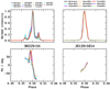 |
Fig. A.1. Stokes-I integrated frequency averaged pulse profiles (top) and PAs against phase (bottom) of PSR B0329+54 and PSR J0139+5814 observed at Band 4. See text for details. |
We plot the phase aligned Stokes-I integrated pulse profiles pulsars PSR B0329+54 and PSR J0139+5814 in the top row of Figure A.1. Each line is color-coded by the day of observation. Reference refers to the EPNDB 610 MHz profiles. The bottom panel shows the matched PA against phase curves. We verify our PA correction and measurement by noticing that when we transfer PA correction from PSR B0329+54 to PSR J0139+5814 on observations 01mar2021, 02mar2021, 12nov2022, 31dec2022 and 18feb2023, all the PSR J0139+5814 PA phase curves agree. Such an agreement is not expected and strongly convinces us that we have taken care of any intra-observation PA rotations.
A.2. DPHASE modeling
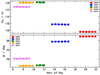 |
Fig. A.2. Variability of DPHASE parameters, Dns and ψr, which are computed using noise diode scans from different MJDs plotted against Hour of Day when the scan was taken. The sign of Dns is purely by convention. |
As uGMRT is an interferometer, it requires phasing of the antennas at regular intervals to produce and maintain a coherent beam on the source. Here, we check if our DPHASE linear modeling is valid from scan to scan within an observation. Figure A.2 shows ψr and Dns measurements from multiple noise diode scans taken during multiple observations. The consistency not just in Dns, but also in ψr implies uGMRT has a stable polarization response within an observation. Incorrect Dns directly impacts RM measurements and unstable ψr affects PA measurements. (Also see Figures B1 and B2 of SB24).
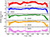 |
Fig. A.3. Deviations from linear DPHASE modeling shown against frequency using noise diode scans taken on different MJDs. Each panel shows deviation where each DPHASE fitted model is subtracted from the DPHASE data. |
The linear DPHASE modeling is simply a model. In every panel of Figure A.3, we show the resultant when linear DPHASE fitted model is subtracted from dataDPHASE for all the noise diode scans we observed in the specific MJD. Since we have multiple noise diode scans, we show the mean and standard deviation computed for every frequency channel with errorbars. We notice departures from the linear model to be of the order of ±15 deg. We also note the following: (i) the deviations are consistent from scan to scan, and (ii) every observation has different form of deviation. As mentioned in the main text, the impact of these unmodeled deviations on the resultant PA is insignificant. When averaged over the entire band, these deviations only change the averaged PA by order of 1 deg.
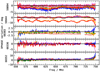 |
Fig. A.4. Variations of DPHASE from scan to scan shown against frequency for different MJDs. Each panel shows the difference of DPHASE between the first noise diode scan and the nth scan for every observation. |
Even though linear model and deviations from the linear model are consistent from one noise diode scan to another, DPHASE variations from one noise diode scan to another noise diode scan are of the order of ±10 deg. To illustrate this, we subtract the DPHASE data of the first noise diode scan from that of all the remaining noise diodes scans. We show the resultant against frequency for every observation in Figure A.4. We note the following: (i) variations are persistent in all the scans, as seen in MJD 60352 at 750 MHz, (ii) variations are drastic as seen in MJD 59944.
Appendix B: Plots
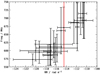 |
Fig. B.1. Bandwidth versus measured RM for a selection of bursts detected on MJD 59243. The bandwidth is shown as error in y-axis, while x-axis error refers to RM error. The red line is the inverse variance weighted RM average. Bursts have been selected such that they occupy around half of the entire observing band. The observed trend is non physical and caused by DPHASE deviations from the linear model used to calibrate. See Sect. 2.2. |
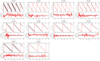 |
Fig. B.2. Outcomes of fitting one RM and one PA to all the bursts from an observation. Each plot corresponds to one observation. The top panels show PA against λ2 − λc2 where λc is the wavelength of the center frequency of the band. The individual data points are shown with black dots and the red line corresponds to the fitted model. The top x-axis shows frequency in MHz. The bottom panels show averaged error between data and fitted model. The horizontal black line is drawn at 0 deg. |
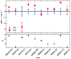 |
Fig. B.3. Difference between one RM fitted to all bursts in an observation (shown with one as legend) and the inverse variance weighted average of each individual QU-fitted RM measurements from each burst of the observation (shown with wrm as legend). The top panel only shows the difference with error-bars. The bottom panels shows the significance of difference. The horizontal black dotted line is drawn at 3σ. The number in parenthesis refers to the number of bursts detected in the respective MJD. |
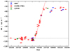 |
Fig. B.4. Rotation measure versus MJD. CHIME/FRB measurements (Mckinven et al. 2023; Ng et al. 2025) are shown in red circles and LOFAR measurements (Gopinath et al. 2024) are shown in green diamonds. GMRT points, shown in blue squares, are the fitted RM values presented in Table 1. |
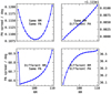 |
Fig. B.5. Showing by means of simulation that spread in PA is only minimized when bursts have a non-varying RM and PA. We simulated 15 bursts with same RM and same PA (top left), same RM but different PA (top right), different RM but same PA (bottom left), and different RM and different PA (bottom right). In each of the cases, we corrected for one RM and measured the spread in PA after correction, which is plotted with blue dots in each of the subplots. The spread in PA is greatly minimized and appears similar to a parabola only in the case of same RM and same PA. |
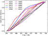 |
Fig. B.6. Cumulative distributions of the bursts of an observation over frequency band. The black bold line is the cumulative uniform distribution. Bursts from every observation occupy the whole observing band. |
Appendix C: Slow precession simulation
In the inertial coordinate system defined in the main text (Sect. 4.3, only the observer axis and the angular momentum axis are constants of motion. The emission axis, however, varies with time in the inertial frame. The angles between the projections of emission axis and angular momentum axis onto the plane perpendicular to the observer axis is defined as the PA. We note that this requires the emission axis to be in the same inertial frame as the observer axis. The projection of the angular momentum axis onto the same plane serves as a reference PA (PA0). We bring the emission axis defined in the body-fixed frame using (α and ϕ0) into inertial frame using Euler angles (ϕ, θ, ψ) where the angles may or may not be functions of time. The Euler angles are defined in ZXZ format. The formalism here is similar to Sect. 37 of Landau & Lifshitz (1976) and that used in Heyl et al. (2024). The θ = δ, that is, it is the spin misalignment angle. ϕ and ψ track the rotational and precessional phase longitudes respectively. Therefore, ϕ and ψ are defined as the following:
where t is the time and Pspin and Ppre are the spin and precessional periods respectively. We note how ϕ0 can be re-defined as the initial value of the ϕ as both are degenerate. There may also be a precessional phase offset which we have omitted here for simplicity.
For the toy model, we set δ = 10 deg, Ψ0 = 0 deg, α = 4 deg, ϕ0 = 200 deg and ζ = 90 deg. Moreover, we set spin period and precessional period to be 10 and 1000 days respectively. Then, we measure the PAs for different spin phases and cycles. We illustrate the PA versus spin phase for different spin cycles in Figure C.1 (top). The different colors imply different spin cycles. We identify three unique spin phases (which we marked with vertical dotted lines of different colors) and plot the PA versus spin cycle at each of the spin phases in bottom panel of the same figure. We highlight that a slow precession model shows intra-cycle variability (variability over spin phase) and inter-cycle variability in the form of sinusoids (variability over spin cycle). The period of the sinusoids is the same irrespective of the spin phase but the amplitude varies.
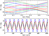 |
Fig. C.1. Outcomes of fitting one RM and one PA to all the bursts from an observation. Each plot corresponds to one observation. The top panels show PA against λ2 − λc2 where λc is the wavelength of the center frequency of the band. The individual data points are shown with black dots and the red line corresponds to the fitted model. The top x-axis shows frequency in MHz. The bottom panels show averaged error between data and fitted model. The horizontal black line is drawn at 0 deg. |
All Tables
Position angle offsets determined from pulsars PSR B0329+54 and PSR J0139+5814 but from the same observation.
All Figures
|
Fig. 1. Applying one RM to all the bursts detected during the observation of MJD 59243 and measuring the standard deviation of all the PA measurements from every time bin of every burst. Repeating this procedure for multiple RMs yields the black dots. The blue line is the fitted parabola. The vertical black line is the center of the fitted parabola. The red dashed vertical line is the RM measured after fitting using all the bursts. See Table 1 and Sect. 2.2. |
| In the text | |
|
Fig. 2. PA∞ values of every time sample of each burst plotted one after the another in individual subplots for every MJD. Each PA∞ has been rotated by ⟨PA∞⟩ taken from Table 1. The different colors indicate different bursts. The shaded region around it is ΔPA, as reported in Tab. 1. The top left text in each subplot is the corresponding MJD and the number of bursts in parenthesis. |
| In the text | |
|
Fig. 3. ⟨PA∞⟩ versus MJD. The points are color coded according to their corresponding activity cycle. |
| In the text | |
|
Fig. 4. ⟨PA∞⟩ versus activity phase of FRB 20180916B plotted with markers with a black border. PA∞ versus activity phase of the bursts plotted with faint markers. Both PA∞ and ⟨PA∞⟩ have been rotated by 45 deg. |
| In the text | |
|
Fig. 5. ⟨PA∞⟩ versus activity cycle for the two phase clusters: G1 and G2. G1 refers to the ⟨PA∞⟩ measurements made at around Phase 0.359 (MJD 59894, 60303 and 60352) and G2 at around Phase 0.400 (MJD 59274, 59568, 59944, 59993). See Sect. 3.2. The black markers are used to denote those ⟨PA∞⟩ measurements with only one burst. The top x-axis shows MJD of the ⟨PA∞⟩ measurements. We emphasize that the reference MJD of the top x-axis is that of the periodicity model of FRB 20180916B. |
| In the text | |
|
Fig. 6. Illustration of rotation (left) and precession (right) geometries considered here. The left image is shown in the inertial coordinate system, which is fixed at the center of the neutron star. The right image is shown in the body fixed coordinate system. The X-axis is toward the right. The Z-axis is up. In case of rotation (left), the rotation axis is along Z-axis. In case of precession (right), the precession axis (symmetric axis) is along Z-axis. Motion is illustrated with large dashed line having arrows at regular intervals. The measured PA is appropriately marked. |
| In the text | |
|
Fig. 7. Position angle measurements of bursts detected by APERTIF at 1370 MHz in activity cycle-37 and -38 (Pastor-Marazuela et al. 2021). Line connecting squares denotes measurements taken in the same observing session. The black dotted line is drawn for every four hours of phase-separation. |
| In the text | |
|
Fig. A.1. Stokes-I integrated frequency averaged pulse profiles (top) and PAs against phase (bottom) of PSR B0329+54 and PSR J0139+5814 observed at Band 4. See text for details. |
| In the text | |
|
Fig. A.2. Variability of DPHASE parameters, Dns and ψr, which are computed using noise diode scans from different MJDs plotted against Hour of Day when the scan was taken. The sign of Dns is purely by convention. |
| In the text | |
|
Fig. A.3. Deviations from linear DPHASE modeling shown against frequency using noise diode scans taken on different MJDs. Each panel shows deviation where each DPHASE fitted model is subtracted from the DPHASE data. |
| In the text | |
|
Fig. A.4. Variations of DPHASE from scan to scan shown against frequency for different MJDs. Each panel shows the difference of DPHASE between the first noise diode scan and the nth scan for every observation. |
| In the text | |
|
Fig. B.1. Bandwidth versus measured RM for a selection of bursts detected on MJD 59243. The bandwidth is shown as error in y-axis, while x-axis error refers to RM error. The red line is the inverse variance weighted RM average. Bursts have been selected such that they occupy around half of the entire observing band. The observed trend is non physical and caused by DPHASE deviations from the linear model used to calibrate. See Sect. 2.2. |
| In the text | |
|
Fig. B.2. Outcomes of fitting one RM and one PA to all the bursts from an observation. Each plot corresponds to one observation. The top panels show PA against λ2 − λc2 where λc is the wavelength of the center frequency of the band. The individual data points are shown with black dots and the red line corresponds to the fitted model. The top x-axis shows frequency in MHz. The bottom panels show averaged error between data and fitted model. The horizontal black line is drawn at 0 deg. |
| In the text | |
|
Fig. B.3. Difference between one RM fitted to all bursts in an observation (shown with one as legend) and the inverse variance weighted average of each individual QU-fitted RM measurements from each burst of the observation (shown with wrm as legend). The top panel only shows the difference with error-bars. The bottom panels shows the significance of difference. The horizontal black dotted line is drawn at 3σ. The number in parenthesis refers to the number of bursts detected in the respective MJD. |
| In the text | |
|
Fig. B.4. Rotation measure versus MJD. CHIME/FRB measurements (Mckinven et al. 2023; Ng et al. 2025) are shown in red circles and LOFAR measurements (Gopinath et al. 2024) are shown in green diamonds. GMRT points, shown in blue squares, are the fitted RM values presented in Table 1. |
| In the text | |
|
Fig. B.5. Showing by means of simulation that spread in PA is only minimized when bursts have a non-varying RM and PA. We simulated 15 bursts with same RM and same PA (top left), same RM but different PA (top right), different RM but same PA (bottom left), and different RM and different PA (bottom right). In each of the cases, we corrected for one RM and measured the spread in PA after correction, which is plotted with blue dots in each of the subplots. The spread in PA is greatly minimized and appears similar to a parabola only in the case of same RM and same PA. |
| In the text | |
|
Fig. B.6. Cumulative distributions of the bursts of an observation over frequency band. The black bold line is the cumulative uniform distribution. Bursts from every observation occupy the whole observing band. |
| In the text | |
|
Fig. C.1. Outcomes of fitting one RM and one PA to all the bursts from an observation. Each plot corresponds to one observation. The top panels show PA against λ2 − λc2 where λc is the wavelength of the center frequency of the band. The individual data points are shown with black dots and the red line corresponds to the fitted model. The top x-axis shows frequency in MHz. The bottom panels show averaged error between data and fitted model. The horizontal black line is drawn at 0 deg. |
| In the text | |
Current usage metrics show cumulative count of Article Views (full-text article views including HTML views, PDF and ePub downloads, according to the available data) and Abstracts Views on Vision4Press platform.
Data correspond to usage on the plateform after 2015. The current usage metrics is available 48-96 hours after online publication and is updated daily on week days.
Initial download of the metrics may take a while.