| Issue |
A&A
Volume 702, October 2025
|
|
|---|---|---|
| Article Number | A65 | |
| Number of page(s) | 17 | |
| Section | Stellar atmospheres | |
| DOI | https://doi.org/10.1051/0004-6361/202556407 | |
| Published online | 07 October 2025 | |
Barium isotopic ratios in metal-poor stars: Calibrating the method with globular clusters
I. Dwarf and giant stars in NGC 6752★
1
INAF – Osservatorio Astrofisico di Arcetri,
Largo E. Fermi 5,
50125
Firenze,
Italy
2
Institut d’Astronomie et d’Astrophysique, Université libre de Bruxelles,
CP 226, Boulevard du Triomphe,
1050
Brussels,
Belgium
3
Royal Observatory of Belgium,
Avenue Circulaire 3,
1180
Brussels,
Belgium
★★ Corresponding author: This email address is being protected from spambots. You need JavaScript enabled to view it.
Received:
14
July
2025
Accepted:
14
August
2025
Abstract
Context. In recent years, the abundances of heavy elements have been proven essential in several major topics in astrophysics, ranging from stellar age determinations to constraining the origins of gravitational wave events, such as neutron star mergers. However, identifying the nucleosynthesis processes behind heavy-element enrichment in stellar atmospheres is challenging. It typically relies on comparing observed abundance-to-iron ratios with theoretical predictions relative to the Sun, but this method is prone to uncertainty due to the limitations of classical 1D hydrostatic models that neglect chromospheric effects. One promising, but still underexplored approach is to measure the isotopic composition of stellar atmospheres by focussing on elements that have both slow (s)-process and rapid (r)-process contributions. While the study of total elemental abundances offers a simplified view, isotopic ratios are directly linked to the underlying nucleosynthesis processes.
Aims. Our aim is to provide a reliable method for quantifying the contributions of the s- and r-processes to the abundance of barium in stellar atmospheres. This can be achieved by determining barium isotopic ratios using 1D atmospheric models in combination with a carefully calibrated microturbulence, based on the comparison between subordinate and resonance Ba lines.
Methods. In this initial study, we used member stars of the globular cluster NGC 6752, assuming a low spread in the Ba abundance, to calibrate the microturbulence (υmic) value for both subordinate and resonance barium lines across different stellar evolutionary stages. This allowed us to provide a reliable estimate of υmic that can be used to accurately determine barium abundances and isotopic ratios in stars ranging from the main sequence (MS) to the upper red giant branch (RGB).
Results. The microturbulence scale adapted for barium subordinate lines for the determination of Ba abundances is consistent with that derived from hydrodynamic (3D) model atmospheres; thus, the Teff-log g dependent relations of the later can be used safely. The microturbulence for the resonance line at λ4934 Å for the determination of the isotopic ratio is higher and depends on the equivalent width (EW). Here, we provide calibrated relations between υmic and EW for measuring isotopic ratios. Regarding the chemical characterisation of the cluster, stars across all evolutionary stages exhibit a clear dominance of the s-process.
Conclusions. Measuring the abundance of heavy elements has proved increasingly necessary, especially in anticipation of new surveys and instruments. In this work, we have provided a practical tool for measuring both the abundance and isotope ratios of Ba, directly related to the EW intensity, and applicable to 1D model atmospheres.
Key words: stars: abundances / stars: atmospheres / stars: Population II / globular clusters: individual: NGC 6752 / globular clusters: general
Based on data of the Gaia-ESO survey.
© The Authors 2025
 Open Access article, published by EDP Sciences, under the terms of the Creative Commons Attribution License (https://creativecommons.org/licenses/by/4.0), which permits unrestricted use, distribution, and reproduction in any medium, provided the original work is properly cited.
This article is published in open access under the Subscribe to Open model. This email address is being protected from spambots. You need JavaScript enabled to view it. to support open access publication.
1 Introduction
Barium is primarily synthesised in the interiors of asymptotic giant branch (AGB) stars through the slow neutron-capture process (s-process). However, numerous stars exhibiting enrichment in elements associated with the rapid neutron-capture process (r-process) have also been found to show enhanced barium abundances (e.g. Hansen et al. 2018; da Silva & Smiljanic 2025). In this context, determining barium isotopic ratios from resonance lines offers considerable potential as a precise diagnostic tool for identifying the underlying astrophysical nucleosynthesis processes; for example, by constraining the relative contribution of the r-process across different environments. The method has
been successfully applied in dwarf stars (Mashonkina & Zhao 2006), where its diagnostic of the r-process contribution aligns well with the results inferred from [Eu/Ba] ratios. Its application to giant stars has also been explored, although it has thus far been largely limited to carbon-enhanced metal-poor (CEMP) stars by several groups (e.g. Meng et al. 2016; Cescutti et al. 2021; Wen et al. 2022).
Nonetheless, the limited use of Ba lines as diagnostic tools in giant stars may be attributed to their tendency to appear strong or saturated, being placed in the non-linear regime of the curve of growth. In Fig. 1, we give an example, displaying the theoretical curves of growth of two Ba resonance lines, obtained from MARCS model atmospheres (Gustafsson et al. 2008). It is well established that one-dimensional (1D) model atmospheres struggle to accurately reproduce such strong spectral lines; not only in terms of their depth and width, but also in capturing the asymmetries between their red and blue wings, which are influenced by granulation effects (e.g. Asplund et al. 2000). Therefore, strong lines are typically avoided in abundance analyses based on 1D model atmospheres, due to their inherent limitations.
The most robust Ba isotopic ratio measurements in very metal-poor ([Fe/H]1 < − 2 dex) giant stars are those of Sitnova et al. (2025). They carefully selected field stars at the base of the red giant branch (RGB) (log g ≲ 2.5 dex), whose Ba resonance lines remain below the plateau of the curve of growth. These stars have reduced equivalent widths (REW2) of ≲ −4.6, see Fig. 1 ; thus, their measurements are virtually unaffected by the 1D modelling biases.
A key aspect to consider in the modelling of Ba lines is the determination of the microturbulence (υmic). This parameter has a substantial impact on the determination of the barium abundance in RGB stars. More importantly, it affects the determination of isotopic ratios both directly and indirectly: directly by influencing the line profile shapes, and indirectly through its impact on the derived barium abundance. Therefore, a dedicated and accurate determination of υmic (specifically tailored to the Ba lines) is essential. In resonance lines, lower υmic induce isotopic ratios diagnoses closer to the r-process. This is because for a fixed υmic value, spectral synthesis requires a source of line enhancement to fit the observational line profile. This could either be the barium abundance or the isotopic ratios. Thus, when a reasonably accurate abundance is determined from subordinate lines (which are insensitive to isotopic ratios variation), and it is fixed to determine the isotopic ratios in resonance lines, the only source of line enhancement is the isotopic ratios. Therefore, since the ratios corresponding to the r-process enhance the line profiles more than those of the s-process (see Fig. 2), the isotope diagnoses tend to be biased toward the r-process. In other words, adopting a low υmic that is not appropriate for resonance lines can lead to misleading diagnoses, artificially biasing the inferred isotopic ratios toward an r-process signature.
In spectral analyses using 1D model atmospheres, υmic is understood as a velocity field that acts on the line opacity, inducing a broadening effect that most strongly affects lines of moderate strength (e.g. Takeda 2022); specifically, those in the flat part of the curve of growth (see Fig. 1). Because of this, υmic is often calibrated by requiring the abundances obtained from weak and moderately intense lines to be consistent regardless of their EW or REW. Steffen et al. (2013) provided a local thermodynamic equilibrium (LTE) υmic validation for RGB stars of solar metallicity based on 3D atmosphere models, where values correlated with Teff remaining between 1 and 1.4 km s−1 are obtained. Dutra-Ferreira et al. (2016) carried out a similar study and determined an empirical relation as function of Teff and log g based on 3D models (for stars with solar metallic-ity), which mostly returns no larger values than 2 km s−1 for stars with log g < 1 dex. However, works in the literature often show values close or slightly larger than 2 km s−1 (e.g. Hansen et al. 2015, 2018; Aoki et al. 2025, among many others). For instance, in the analysis of the best studied metal-poor RGB star, the Gaia Benchmark HD 122563, four spectroscopic algorithms provide consistent values of vmic derived from iron lines close to 1.9 km s−1 (Jofré et al. 2014).
Even assuming the ideal scenario where υmic is accurately determined from Fe lines, the crucial question is whether this value is also appropriate for modelling Ba lines, given their different line strengths and formation depths. The likely reason for a negative answer is the influence of chromospheric layers, which can alter the formation of strong Ba lines in ways not captured by standard photospheric models typically used to derive υmic from Fe lines. A detailed discussion on this topic is provided by Reddy & Lambert (2017), who examined evidence related to the formation depths of strong Ba lines. They demonstrated that for the solar case, depths based on calculations using 1D models (Mashonkina et al. 1999; Mashonkina & Zhao 2006) can appear significantly deeper than those derived from empirical photospheric models tailored to the Sun (Gurtovenko & Sheminova 2015). The authors consider this discrepancy as an evidence of barium abundance biases induced by the simplified hydrostatic approximation in stars with spectra modulated by their chromosphere. In most RGB stars, the subordinate Ba lines are oversaturated (REW ≳ −4.6), whereas the resonance lines remain in the damping region of the curve of growth (REW ≳ −4.5; see Fig. 1). These lines are notably strong, and their cores therefore probe higher atmospheric layers than those of saturated Fe lines. As a result, the influence of chromospheric layers on the barium lines might be manifested through an irregular response to the microturbulent velocity derived from Fe lines. This problem has been known as the barium puzzle (D’Orazi et al. 2009, 2012), which is manifested as barium abundance excess observed especially in RGB stars and young dwarfs relative to old dwarfs in open clusters of solar-like metallicity (e.g. Baratella et al. 2020, 2021). The analysis from Reddy & Lambert (2017) demonstrated a correlation between the Ba excess and the chromospheric activity of young stars, but it can be present also in non-active stars as an effect of the incorrect choice of the microturbulent velocity in the spectral analysis. Therefore, the apparent Ba excess measurements are probably biases related to spectroscopic methods.
In this work, our goal is to establish a well-calibrated method for determining microturbulence for the different Ba lines of a wide range of strength, and to provide a straightforward prescription to infer it from the microturbulence typically obtained from Fe lines. We confirm, with observational evidence, that strong Ba lines require υmic values different to those from Fe lines, as previously indicated by Reddy & Lambert (2017).
In this first paper (Paper I), we present the analysis of a sample of member stars in the globular cluster NGC 6752, taking advantage of their expected homogeneity in terms of age and metallicity. The sample includes both dwarf and giant stars, allowing us to calibrate the microturbulence parameter required to obtain consistent Ba abundances along the cluster’s evolutionary sequence. As shown in Fig. 1, the strengths of resonance lines we are analysing (λ4934 Å) in our stars cover the three regions of the curve of growth. The damping region is the one of the greatest interest, since most metal-poor stars (including CEMP ones) are expected to have resonance lines of a similar strength.
In Paper II, we will apply the calibrated relations between stellar parameters and microturbulence to derive Ba abundances and isotopic ratios in a larger sample of metal-poor field stars. Finally, in Paper III, we will analyse a sample of 14 globular clusters, as presented in Schiappacasse-Ulloa et al. (2025), deriving Ba abundances and isotopic ratios, and correlating them with the clusters’ stellar populations.
The structure of the paper is as follows: in Sect. 2, we describe the selection of our stellar sample. Sect. 3 outlines the derivation of the stars’ atmospheric parameters. In Sect. 4, we detail the method used to calibrate the microturbulent velocity specifically for barium lines. Sect. 5 presents the derived barium abundances and isotopic ratios, along with a discussion of how these diagnostics may relate to the hypothesis of multiple stellar populations. In Appendix F, we compare our metallicity scale with values reported in the literature and discuss the implications in the context of atomic diffusion. Finally, Sect. 6 summarises our main findings and conclusions.
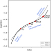 |
Fig. 1 Theoretical curves of growth for the two Ba resonance lines. Equivalent widths (EW) were computed in spectra synthesised by MARCS 1D atmosphere models adopting the atmospheric parameters Teff = 5540 K, log g = 2.45, [Fe/H] = −2.00 dex, and υmic = 1.5 km s−1. The barium abundance in the horizontal axis is neglected on purpose, as the scale depends on the abundance itself and the stellar parameters. The location of our stars is indicated by the red circles, where they are designated according to their evolutionary state as follows: turn-off (TO), subgiant (SG), base of the red giant branch (bRGB), over the clump RGB (ocRGB), and upper RGB (uRGB). |
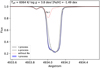 |
Fig. 2 Synthetic profiles of the line at λ4934 Å. The synthesis was made with the Turbospectrum code (Gerber et al. 2023) and MARCS models. See details in Sect. 5.2. The atmospheric parameters for the synthesis are similar to those of the star GES J19102677-6003089 (TO-1) in Table 2. The spectrum has resolution R = λ/∆λ = 493 000 and infinite S/N. The solid line (r-process), dashed line (s-process), and blue shade (i-process) profiles are synthesised with the isotopic ratios in Table 5. |
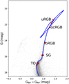 |
Fig. 3 Colour-magnitude diagram of NGC 6752. Grey and red symbols represent stars in the cluster field and the sample analysed in the present work, respectively. Photometry for both samples was taken from Gaia eDR3. An isochrone of 12 Gyr is overplotted as a reference. |
2 Data and sample
We present a sample of 14 stars belonging to the globular cluster NGC 6752, spanning a broad range of evolutionary stages, from dwarf main sequence turn-off stars to RGB stars. Specifically, we selected stars in five regions of the Kiel diagram: turn-off (TO), subgiant (SG) branch, base of the RGB (bRGB), over the clump RGB (ocRGB), and upper RGB (uRGB); the locations of these regions are indicated in Fig. 3. The grey dots represent stars located in the field of NGC 6752, selected from the Gaia eDR3 data within a circular radius of 10 arcmin. We note that these stars were intended to guide the eye and are not necessarily members of the cluster. Red dots represent the stars analysed in the present article, and the blue line is the PARSEC isochrone (Bressan et al. 2012) for [M/H]=−1.25 dex, [α/Fe]=0.35 dex, an age of 12.0 gigayears (Gyr), (m-M)0=13.13, and an extinction of 0.04. The whole sample has Ultraviolet and Visual Echelle Spectrograph (UVES) spectra retrieved from the ESO archival data, covering a wavelength range of 480-680 nm. With the exception of 19111828-6000139, these stars were analysed by the Gaia-ESO survey (Gilmore et al. 2022; Randich et al. 2022) as part of its calibration programme, which also included several open clusters, benchmark stars, and asteroseismic targets. For a detailed overview of the calibration sample, as well as the global calibration and survey homogenisation process, we refer to Pancino et al. (2017) and Hourihane et al. (2023). Among the stars in this cluster observed by Gaia-ESO, we selected those having spectra with the highest signal-to-noise ratio (S/N). To validate the chemical abundances determined for our two TO stars, we also analysed spectra from two additional TO stars, despite their lower S/N.
To ensure that the selected stars are bona fide members of NGC 6752, we included only those with a membership probability (M-PROB) greater than 0.99, following Vasiliev & Baumgardt (2021). These findings are aligned with the membership probabilities reported in Gaia-ESO Data Release 5.1 (DR5.1) (Hourihane et al. 2023), which were determined by combining proper motions and parallaxes from Gaia with radial velocities derived from Gaia-ESO. For further details on the membership determination process, we refer to Jackson et al. (2022).
Table 1 provides key information on our sample stars, including co-ordinates (RA and Dec), [Fe/H], and radial velocity (Vr) from Gaia-ESO, proper motions, and parallaxes (ω̄) from Gaia eDR3, and S/N.
NGC 6752 sample information.
3 Atmospheric parameters
As a first step, we redetermined the stellar parameters of our sample using techniques that deliver high precision for every parameter.
3.1 Determination of Teff
We determined Teff by averaging the outcomes of two methods: Balmer Hα line modelling and applying the Gaia colour-Teff relations of Casagrande et al. (2021) based on the infrared flux method (IRFM, Blackwell et al. 1979); we refer to the latter as the photometric Teff. We included the latter because the spectra of our TO dwarf stars have low S/Ns; thus, their Hα Teff results might be less precise. The Teff scales of both methods are consistent (Giribaldi et al. 2021, 2023); thus, any differences in the values derived here likely arise from external sources of uncertainty, such as photometric errors, extinction, or residual instrumental patterns in the spectra.
The observational Hα profiles were normalised and fitted to 3D non-LTE (NLTE) synthetic grids (Amarsi et al. 2018) using the method of Giribaldi et al. (2019, 2021, 2023). We derived photometric Teff from the Gaia colours GBP – GRP and G – GBP, as these have been shown to provide the most accurate results (Giribaldi et al. 2023). The colours were corrected by subtracting the extinction E(B – V) = 0.04 determined by Gratton et al. (2001), which was transformed into the Gaia system using the coefficients of Fitzpatrick (1999). This approach was explained in Casagrande et al. (2021) and implemented in the COLTE3 routine. The final Teff is computed as the weighted mean of the temperatures derived by the two methods, with the weights given by the inverse square of their respective uncertainties. The uncertainties of the temperatures derived from Hα were estimated based on the fitting errors associated with the spectral noise. For the uncertainties of the temperatures derived from the colour-Teff relations, we adopted a constant error of 100 K, which accounts for the intrinsic precision of the relations themselves (70-80 K) and the combined uncertainties in the photometric colours and extinction estimates (~30 K). Total errors are computed following Eq. (1) in Giribaldi et al. (2025) considering a minimum error of 30 K. The photometric temperatures derived from G – GBP for some stars differ significantly from those obtained via GBP – GRP and Hα. This discrepancy may result from biases in the measured magnitudes. Table A.1 lists the stellar temperatures derived using each method.
3.2 Determination of log g
We determined log g by searching for the excitation equilibrium of neutral and ionised Fe lines under NLTE (log gNLTE); we also determined log g under LTE for comparison (log gLTE). For that, we performed line synthesis using the radiative transfer code Turbospectrum 20204 (Gerber et al. 2023) with MARCS model atmospheres (Gustafsson et al. 2008). We considered the atomic parameters from Heiter et al. (2021) and the iron NLTE departure coefficients based on the model atom developed in Bergemann et al. (2012) and Semenova et al. (2020). We assumed excitation equilibrium to compute the surface gravity, following the findings of Giribaldi et al. (2023), who showed that Fe I and Fe II lines yield consistent NLTE abundances when log g is fixed to the value independently derived from the Mg I b triplet.
3.3 Determination of [Fe/H] and υmic
We determined the metallicity and υmic by applying the spectral synthesis method to the lines contained in the line lists of Jofré et al. (2014). For giants, we used the line list adopted for HD 122563 and HD 220009 in that paper, to which we added six Fe II lines from Meléndez & Barbuy (2009), namely, the lines at λ 5018.43, 5169.028, 5234.62, 5362.86, 5425.26, and 5534.83 Å. For dwarfs, we combined the line lists used for metalpoor stars in Jofré et al. (2014), to which we added the six lines above. Figure 4 shows the location of our sample stars in the Kiel diagram, where the evolutionary stages are labelled. Isochrones with slightly varying ages and metallicities are overplotted for reference. The diagram compares log gNLTE and log gLTE, illustrating that the assumption of excitation equilibrium under LTE results in significantly underestimated surface gravities. Our final adopted stellar parameters are Teff, log gNLTE, and [Fe/H]NLTE.
Atmospheric parameters of the NGC 6752 stars.
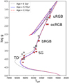 |
Fig. 4 Kiel diagram of the program stars. Red circles display Teff and log gNLTE. Gray circles display log gLTE. Quantities are listed in Table 2. |
3.4 Evaluation of biases in the determination of υmic
Our ultimate goal is to assess whether υmic values derived from Fe lines can be reliably applied to both subordinate and resonance Ba lines – or whether it requires adjustment through calibrated relations, under the initial assumption that the stars in the cluster exhibit a negligible intrinsic spread in barium abundance.
The first step is to evaluate potential biases and to identify and exclude outlier lines, aiming to define the best set of lines to derive υmic. To this end, we derived [Fe/H] and υmic from the iron lines using two different methods. The former method is based on the application of the ionisation balance. It consists of deriving an average [Fe/H] from individual line-by-line measurements. In this process, the Teff is kept fixed, while the log g, υmic, and macroturbulent velocity (υmic) are allowed to freely vary. These parameters are adjusted until no correlation is found between the individual [Fe/H] values and REWs. We imposed an upper limit to REW < −4.8 to exclude any oversaturated lines. We provided both LTE ( ) and NLTE (
 ) determinations from this method. In the latter method, we performed a global fit by simultaneously fitting all Fe lines with REW less than −4.8, using LTE synthetic spectra. In this approach, [Fe/H]fit,LTE,
  , and vmac were treated as free parameters, while log gLTE and Teff were kept fixed. All the parameters are listed in Table 2.
We took special care in carrying out the spectral normalisation because it is one of the most important factors influencing the microturbulence determination. We applied local normalisation by selecting wavelength chunks of ±1 Å around the line centre. This practice is reliable in spectra of moderate-resolution of metal-poor stars because their metal lines are frequently surrounded by continuum regions of reasonable extension. We rejected lines that are too noisy or likely to be blended with other features. For that end, we fitted the lines with Gaussian functions and supervised their fitting quality using the minimum χ2 test. We observed that for every star, the dispersion of χ2 decreases with the wavelength; this is likely because the S/N increases. For giant and subgiant stars, we excluded lines with χ2 values exceeding the 75th percentile. An example is shown in Fig. G.1 in the appendix. In the spectra of dwarf stars, Fe lines are scarce, not only because their higher temperatures, but also because the spectral noise is higher. For these stars, we supervised the fits manually on a line-by-line basis and excluded those with insufficient quality. Thus, we maximised the selection of well-shaped lines obtaining a total of 45 ones. Once a spectrum with locally normalised Fe lines was produced and low-quality lines were clipped from the lists, we applied the two methods above to derive [Fe/H] and vmic. This approach ensures that any differences in the results are solely attributed to the methods themselves.
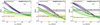 |
Fig. 5 LTE barium abundance as function of υmic for the subordinate lines 5853, 6141, and 6496 Å. Each trend is related to one star and is colour-coded according to log g. Shades enclose the most probable ranges of A(Ba) of the TO-1 and TO-2 stars; see main text. Dashed gray and red lines indicate the mean A(Ba) in the shades for each star, respectively. |
4 Microturbulence adapted to barium lines
The fundamental premise underlying the present work on calibration is the theoretical expectation of homogeneity in the Ba abundance of the cluster, irrespective of the evolutionary stage of the stars. In reality, the situation proves to be considerably more complex than initially anticipated. In particular, A(Ba) of TO stars has been reported to be lower than in RGB stars by ~0.15 dex in the metal-poor cluster NGC 6121 (Nordlander et al. 2024). The microturbulence calibrations we present in this work are computed considering an overall abundance uncertainty that cover such potential variation in case it is authentic.
Additionally, the two turn-off stars with the highest S/N (TO-1 and TO-2), initially intended to serve as proxies, exhibit different barium abundances and isotopic ratios. For this reason, we carried out a posterior validation step, that included two additional TO stars, even though their spectra have much lower S/N. These stars were used to identify the anomalous star among TO-1 and TO-2. In Section 5.3, we briefly discuss some hypotheses regarding its origin. We refer to Paper III (Schiappacasse Ulloa el al., in prep.) for an in-depth discussion on the relationship between different stellar populations in globular clusters and the isotopic abundance of Ba.
4.1 Subordinate lines
In this section, we investigate the behaviour of the Ba subordinate lines, which are those originating from transitions between excited energy levels, rather than from the ground state. We determined A(Ba)5 in our sample stars by varying υmic in the range 0.8-2.6 km s−1 to quantify the sensitivity of each line to υmic and to examine how this sensitivity varies with the evolutionary stage. Here, this is represented by log g across the five stages. Figure 5 shows the sensitivity of each subordinate line to variations in υmic; corresponding NLTE results are shown in Fig. G.5 in the appendix. The most evident (and anticipated) is that for all lines, the abundance is less sensitive to υmic in TO stars than in RGB stars. Considering the fact that in TO stars, the Ba lines are weak; thus, they are less affected by departures from 1D hydrostatic atmosphere modelling, we assume that their abundances are the closest to the true values. However, in Fig. G.5, we show A(Ba) under 1D NLTE is about −0.2 dex relative to that in 1D LTE. Therefore, the barium abundances of TO-1 and TO-2 might be adopted as the best proxies for the cluster abundance. The detailed determination of their Ba abundances is presented in Section 5. However, as anticipated, we noted that the barium abundance of the TO-2 star is significantly lower than that of TO-1. Moreover, the abundances of TO-3 and TO-4 closely match that of TO-1, although the lower S/N of their spectra results in lower precision. This has important implications, as reproducing the same A(Ba) as in TO-2 in the other stars would require unrealistically high values of vmic.
The plots in Fig. 5 include error shades associated to the A(Ba) ranges of the TO stars obtained when υmic is changed from 1 to 1.5 km s−1. This range was determined with the TITANS I metal-poor dwarfs (Giribaldi et al. 2021), performing LTE synthesis fixing their quoted parameters. Figure G.4 shows the distribution of vmic as functions of the atmospheric parameters. Assuming that the shaded areas in Fig. 5 enclose the true abundances, for every curve in the plots, we computed the υmic ranges corresponding to the enclosed A(Ba) ranges.
Figure 6 shows the vmic ranges computed as functions of Teff (black solid bars) when the A(Ba) of the TO-1 star is assumed as proxy. Each column of the plot corresponds, respectively, to the subordinate lines at λ5853, λ6141, and λ6496 Å in LTE. Orange dashes indicate the medians of the mean values derived from the bars within each evolutionary stage. These median values are shown in the plots alongside their associated uncertainties, computed by summing in quadrature the standard deviation of the bar means and the individual bar errors divided by the number of bars. These median values represent the microturbulence calibrated to the subordinate lines, hereafter referred to as  .
.
The microturbulence from Fe lines listed in Table 2 are shown for comparison; only the errors of  are plotted.
  ,
,  , and
, and  are equivalent for stars at the uRGB and ocRGB stages. At the bRGB and SG,
  is slightly lower than
  by 0.1-0.2 km s−1, whereas
  tend to be even lower. We also over-plot microtubulence values computed by the relation of Dutra-Ferreira et al. (2016) based on 3D LTE models (green dashes). An excellent agreement is observed between these values and
  for all evolutionary stages except for the SG stars. Therefore, for practical purposes, we recommend the use of the relation in Dutra-Ferreira et al. (2016), which is transcribed below in Eq. (1), for safely determining Ba abundances from the subordinate lines,
 (1)
(1)
where X = Teff−5500 and Y = log g −4.0. The root mean square (rms) scatter of this relation is 0.05 km s−1, according to the paper source. Therefore, we adopt this quantity to compute the abundance errors in Sect. 5. Fig. 6 also show  , when the TO-2 star is adopted as the reference for the cluster A(Ba), shown as brown dashes. In this case, the
  values derived from the line at λ6496 Å are significantly higher than those obtained from the lines at λ5853 and λ6141 Å, exceeding 2.5 km s−1 at all evolutionary stages. Although this exercise is intentionally illustrative (anticipating atypical values of
  ), the values obtained for the SG stars (reaching approximately 2.85 km s−1) are particularly suspicious given that the lines are only moderately saturated (REW ≈ −4.9). For bRGB stars, the derived
  becomes unphysically large (>10 km s−1); thus, no corresponding value is shown in the right panel of the plot.
Table 4 presents an example of the variations in A(Ba) induced by changes in υmic across the different evolutionary stages. These values are derived from the behaviour of the line at λ6141 Å, shown in the middle panel of Fig. 6, assuming the TO-1 star as the reference proxy.
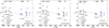 |
Fig. 6 Microturbulence as function of Teff for the stars in Table 1. Panels descriptions, from left to right, are as follows. Quantities derived from the subordinate lines at λ5853, 6141, and 6496 Å, respectively. TO stars are excluded on purpose. Vertical bars represent υmic ranges computed by the intersections of the trends with the shades in Fig. 5. Orange dashes are medians of contiguous bars, which correspond to stars in the stages indicated on the top; these values are defined as |


4.2 Resonance lines
In the previous section, we described how we assessed that the A(Ba) from subordinate lines of the uRGB, ocRGB, and bRGB are compatible with that of TO-1, using the appropriate value of the microturbulent velocity. It is therefore expected that their Ba abundances have the same nucleosynthetic origin (e.g. similar isotopic composition). In Sect. 5.2, we demonstrate that the barium abundance in star TO-1 is entirely produced by the s-process, whereas in TO-2 it is predominantly of an r-process origin. Anticipating this result, we perform for the resonance lines an exercise similar to that done for subordinate lines in Fig. 5. However, instead of fixing only A(Ba) to calibrate the microturbulence, we fixed both A(Ba) and the isotopic ratios, separately testing the ratios corresponding to the r- and s-process contributions. In this way, we can also assess which of the TO stars reflects the typical composition of the cluster and which one shows a peculiar abundance pattern.
Figure D.2 in the appendix displays the trends of A(Ba) as a function of vmic, using as reference the A(Ba) values of TO-1 (representative of the s-process) and TO-2 (representative of the r-process). The shaded regions reflect the abundance uncertainties, calculated by adding in quadrature the contributions from σsn and σT. The uncertainty due to σv was excluded to enhance the precision of our estimates. We obtain microturbulence adapted to the resonance line at λ4934 Å ( ) in an analogous way as in Fig. 6. Figure 7 presents a comparison between the microturbulence values derived from Fe lines and those calibrated using Ba lines. The average values of
  and their associated uncertainties, computed following the method described in the previous section, are indicated in each panel.
In the right panel, where the lower A(Ba) value of TO-2 is taken as representative of the cluster abundance,  exceeds
  by approximately 0.8 km s−1. Notably, this offset does not follow the expected trend of increasing discrepancy with line strength (from right to left in the plot) as would be predicted due to the greater sensitivity of stronger lines to the limitations of 1D atmospheric models, especially in the damping region of the curve of growth. More specifically, the central panel, representing the full r-process, shows discrepancies only at higher Teff, where the lines are weaker. This is contrary to the expected behaviour and, therefore, this calibration attempt is also deemed incorrect.
In contrast, when the higher A(Ba) value of TO-1 is assumed to represent the cluster abundance, the discrepancies are minimised. The left panel, representing 100% s-process isotopic ratios, shows that only the strongest lines (from the uRGB and ocRGB stars) require larger microturbulence values than those derived from Fe lines, as expected. Therefore, the calibration can be considered correct.
This supports our choice of considering TO-1 as representative of the cluster’s Ba abundance and isotopic ratios, and as the reference for calibrating the microturbulence accordingly. The implications of these findings are discussed in the following section. A more effective method is to follow the trend shown by the adapted microturbulence as a function of EW and REW in Fig. 8. The EW and REW are parameters more directly related to line shapes than Teff, making the use of  less likely to fail in cases of Ba variations. A LOWESS6 regression and a polynomial are fitted to
  (red dashes). These are represented by the solid and dashed lines; the equation of the latter is given below:
 (2)
(2)
The uncertainty of the υmic estimates of these trends is of ±0.10 km s−1; it is an approximate quantity to those determined in left panel of Fig. 7. Therefore, we adopted this quantity to errors of the isotopic ratios, as described in Sect. 5. The trends of the LOWESS and the polynomial function are similar. When these are compared with υmic from 3D models (green dashes, which is well suited to the Ba subordinate lines, as demonstrated in Fig. 6), it is evident that  is systematically higher. At the SG and bRGB stages the difference is about +0.1 km s−1, whereas at the uRGB and ocRGB stages the difference increases to about +0.25 km s−1. We recommend using the polynomial in Eq. (2), or the quantities given in the plot, for fixing υmic when determining Ba isotopic ratios from the line at λ4934 Å.
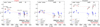 |
Fig. 7 Microturbulence as function of Teff for the line 4934 Å. Left and centre panels shows quantities derived assuming 100 and 0% s-process contributions, respectively. A(Ba) = 1.15 ± 0.08 dex of the TO-1 star is assumed in both cases. Right panel shows quantities derived assuming the A(Ba) = 0.39 ± 0.08 dex and full r-process contribution of the TO-2 star. Black bars represent the microturbulence ranges required to fit observational lines with synthetic ones. Red dashes are the medians of the bars in the stages indicated on the top. The red and blue dotted lines are linear regressions of the red and blue dashes, respectively. |
5 Barium abundance and isotopic ratios
Following the calibration of the microturbulence for the various resonant and subordinate lines of Ba, the abundances of the stars belonging to the cluster can be determined with a high precision.
5.1 Barium abundance
We derived the barium abundance assuming LTE conditions. We performed spectral synthesis fitting the subordinate lines at λ5853, 6141, and 6496 Å. The atomic parameters of the two latter can be found in Gallagher et al. (2020). Details on the hyperfine splitting (HFS) and associated oscillator strength (in logarithmic scale, log gf ) values of these lines are provided in Giribaldi et al. (in prep.). The abundances of the stars are listed in Table 3. The fits are made fixing the microturbulence to the values obtained from Eq. (1). Section 4.1 provides a justification of this choice.
Total abundance errors are given by the following relation,
 (3)
(3)
where σsn is the error related to the noise, σT is the error related to Teff, and σv is the error related to υmic. All these errors are individually annotated in Table 3. Errors induced by typical uncertainties in log g and [Fe/H] are negligible for both dwarfs and giants (i.e. lower than 0.01 dex). Then, σsn is assumed to be the standard deviation of the A(Ba) values obtained from the subordinate lines; σT is computed as described in Giribaldi et al. (2023) using synthetic spectral grids of the line at λ6141 Å as a proxy (see the associated plots in Fig. G.2). Errors related to variations of ±50 K are listed in Table 4. Finally, σv is estimated from the analysis of Sect. 4, where the error of the microturbulence (±0.05 km s−1 ) is given by the rms of Eq. (1). We employed this error and the values in Table 4 to compute σv for each star. The values in the table were computed from vmic versus A(Ba) variations of the sensitive line λ6141 Å (Fig. 5), which was used as proxy.
5.2 Barium isotopic abundance ratios
We determined the Ba isotopic ratios by fitting the profile of the resonance line at λ4934 Å, fixing the abundances determined from subordinate lines.
This resonance line is not included in Gallagher et al. (2020); therefore, we computed a log gifij = gjλ2ijAji/6.6702 × 1015 = −0.172; where gj = 2 is the upper statistical weight of the transition, λij = 4935.45 Å is the wavelength of the transition in vacuum, and Aji is the spontaneous transition probability from De Munshi et al. (2015). The detailed isotopic shifts, HFS, and corresponding log gf values for this line are given in Table B.1. They are based on energy levels in the NIST7 database, and on Silverans et al. (1986); Villemoes et al. (1993); Trapp et al. (2000); Itano (2006) for hyperfine structure constants of odd Ba II isotopes 135 and 137. We employed the isotopic ratios in Table 5 for the s- and r-processes.
Our analysis is based on the premise that heavy elements in the interstellar medium are progressively enriched by nucleosyn-thetic products. Consequently, we interpreted the isotopic ratios as complementary fractions of s- and r-process contributions. We quantified the isotopic ratios in terms of the s-process fraction, ranging from 0% (indicating a pure r-process origin) to 100% (a pure s-process origin), as reported in Table 3. For each star, we assigned the isotopic ratio corresponding to the synthetic profile that (i) reproduces the mean A(Ba) derived from the subordinate lines and (ii) provides the best fit to the observed line profile.
Figure 9 shows the application of the method to the uRGB-1, TO-1, and TO-2 stars, as examples. The syntheses correspond to the A(Ba) listed in Table 3 with the s-process contribution percentage that fits better the observational profile. The plots also display line profiles corresponding to 0 (r-process) and 100% s-process contributions. These are more easily distinguished in the residual plots in the bottom panel. The errors related to the flux variation due to spectral noise are noted within brackets. The inner plots display the χ2 minimisation used for fitting, where the shades cover the errors in brackets. Only for the TO-2 star, the synthetic profile that best fits the observational line corresponds to the r-process.
The uncertainty on the isotopic ratios is primarily driven by the uncertainties in the stellar parameters that most significantly affect the line profiles, and it can be expressed as follows:
![Mathematical equation: \Sigma_{iso} = \sqrt{ \sigma_{sn-iso}^2 + \sigma_{Ba-iso}^2 + \sigma_{T-iso}^2 + \sigma_{v-iso}^2 + \sigma_{[\mathrm{Fe/H}]}^{2} }](/articles/aa/full_html/2025/10/aa56407-25/aa56407-25-eq53.png) (4)
(4)
where σsn-iso is the error related to noise, σBa-iso is the error induced by the A(Ba) errors, σT-iso is the error induced by the Teff errors, σv-iso is the error induced by the vmic errors, and σ[Fe/H] is the error induced by [Fe/H] errors. All these errors are individually listed in Table 3. Details on how the various parameters influence the measurement of the isotopic ratio are provided in Appendix D.
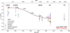 |
Fig. 8 Microturbulence as function of EW and REW for the Ba resonance line at λ4934 Å. Microturbulence values determined from diverse methods are represented according to the legends. The solid black line is the polynomial regression of |

Barium abundances of the NGC 6752 stars.
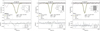 |
Fig. 9 Fits of the 4934 Å Ba resonance line. The stars to which each plot corresponds are indicated in the plots. The observational profiles are represented by the black lines. Synthetic profiles are represented by coloured lines. The synthetic profiles most compatible with the observational ones are represented by the thick olive lines; their s-process contributions are noted along with the errors related to the noise. Synthetic profiles related to s- and r-processes are represented by the dotted or dashed green lines according to the legends. A synthetic spectra without barium are represented by the dotted red lines. The probability for a given process to dominate the line profile shape is given by the χ2 in the inner plot. The shades in the inner plots cover errors of the s-process contribution. Residual plots are shown at the bottom panel, where the shades represent the areas covered by the fitting errors. |
A(Ba) errors induced by Teff and υmic errors.
5.3 Hypothesis on the origin of the two TO stars
Although it is not the primary aim of this paper to analyse the barium abundance and isotopic composition of NGC 6752, but rather to provide calibration relations for microturbulence, we cannot avoid commenting on the TO stars. One of the most intriguing hypotheses is that the lower barium abundance, combined with an isotopic ratio fully dominated by the r-process, could point to a first-generation star within the framework of multiple stellar populations in globular clusters. In fact, one of the most distinctive characteristics of GCs is the presence of multiple stellar populations – a phenomenon observed in nearly all Galactic GCs. The prevailing theory suggests that GCs initially formed a first generation (FG) of stars from pristine gas, namely, gas with the original, unprocessed chemical composition. A subset of these stars, commonly referred to as polluters, then enriched the intracluster medium with elements synthesised during their lifetimes. This enriched material was subsequently mixed with the remaining pristine gas, leading to the formation of a second generation (SeG) of stars. These different stellar populations can be identified through their distinct chemical signatures, particularly in the abundances of hot H-burning elements such as oxygen, sodium, magnesium, and aluminium. Schiappacasse-Ulloa et al. (2022) presented evidence that intermediate-mass AGB stars (4-8 M⊙) contributed to this enrichment in NGC 6752, which might contribute some degree of s-process elements, varying their yields according to the mass and metallicity of the star. However, Schiappacasse-Ulloa & Lucatello (2023) found no significant differences in the abundances of Ba or other s-process elements between the stellar populations, despite observing a substantial spread in Ba. Table 1 lists in the last column the stellar population membership: first generation (FG) or second generation (SeG) – as determined by Na abundances from Schiappacasse-Ulloa et al. (2025). Except for TO-2, none of the stars exhibit statistically significant differences in either A(Ba) or isotopic composition, regardless of their population. This weakens the hypothesis of a systematic difference in isotopic ratios between the two generations. The similar Ba abundances observed in both FG and SeG stars support the findings of Schiappacasse-Ulloa & Lucatello (2023), and also suggest that the anomalous Ba abundance in TO-2 is unlikely to be associated with the multiple population phenomenon.
Another possible hypothesis is that TO-2 is not a cluster member and was accreted at a later stage. However, its metallicity is consistent with that of the other TO stars, and its astrometric and kinematic properties strongly support its membership.
This star will be discussed in greater detail in Paper III, along with the other globular clusters observed as part of the Gaia -ESO survey, and previously presented in Schiappacasse-Ulloa et al. (2025).
6 Discussion and conclusions
To the present day, many CEMP stars are found to be enhanced in both r- and s-processes (usually labelled as CEMP-rs). Hypothetical scenarios explaining how such stars ended up with that specific chemical composition pattern, consisting of either pollution (of the primordial cloud or the already formed star system, e.g. Beers & Christlieb 2005; Jonsell et al. 2006; Hansen et al. 2016; Gull et al. 2018) or an intermediate (i-) speed nucleosynthesis process (Cowan & Rose 1977). The latter has been theoretically investigated (e.g. Choplin et al. 2021; Goriely et al. 2021; Choplin et al. 2022; Martinet et al. 2024; Choplin et al. 2024; Denissenkov et al. 2021). However, no a star exhibiting a chemical pattern that would be consistent with the predictions of the i-process has been identified thus far.
The most rigorous method used to classify CEMP stars into r-, s-, or rs-process subgroups consists of comparing their heavy element abundances with theoretical nucleosynthesis predictions (e.g. Gull et al. 2018; Sbordone et al. 2020; da Silva & Smiljanic 2025). However, the method is prone to inaccurate results from line modelling using classical 1D model atmospheres (under LTE or NLTE) because in CEMP stars (which are mostly RGB) spectral lines are often very intense and also may be severely blended with molecular features. In this context, a competitive alternative method is the determination of isotopic ratios of heavy elements. The barium resonance lines may serve as an effective indicator, as these are shaped according to the dominating nucleosynthesis process. The s-process produces even isotopes (134, 136, and 138) in greater quantities than the r-process, which mostly produces odd isotopes (135 and 137); see Table 5. Since the latter mostly influence the line profile wings, whereas the former mostly influence the line core, their line profiles are certainly distinguishable (see Fig. 2) in spectra of sufficient quality (e.g. Mashonkina & Zhao 2006; Gallagher et al. 2020; Cescutti et al. 2021). Additionally, the i-process shapes a line that is almost identical to that of the r-process (blue shade and solid line in Fig. 2, respectively). Therefore, in this spectral feature, a star where both s- and r-processes dominated should be distinguishable from one where the i-process was dominant.
In principle, it should be somewhat straightforward to model Ba resonance lines via spectral synthesis. However, these are strong in CEMP stars; therefore, their isotopic diagnoses made without considering ad hoc parameter calibrations are unreliable, given that 1D model atmospheres are unsuitable to lines of such strength. To take advantage of this tool of great potential,and to promote its use, we analysed the behaviour of barium lines in metal-poor stars along several evolutionary stages, spanning the turn-off all the way to the upper RGB. For this purpose, we used stars in the NGC 6752 cluster (see Fig. 4), whose A(Ba) abundances are reasonably homogenous (±0.1 dex, e.g. Schiappacasse-Ulloa & Lucatello 2023). This characteristic allowed us to fix the abundance in the spectral synthesis to calibrate microturbulence quantities according to the line strengths. Multiple stars were included at each evolutionary stage (Figs. 3 and 4) to ensure that our conclusions are not based on atypical cases.
Using turn-off stars as A(Ba) reference (fixing the same abundance for all cluster stars), we first calibrated the microturbulence ( ) to several subordinate lines λ5853, λ6141, and λ6496 Å. We did not find substantial differences with υmic computed from Fe lines under 1D LTE; except in the case of SG stars, where
  is lower by ~0.40 km s−1 (see Fig. 6). On the other hand, we find that
  is compatible with the 3D model-based microturbulence provided by the Teff-log g dependent relation of Dutra-Ferreira et al. (2016), which is reproduced in Eq. (1).
We recommend the use of that relation for the determination of the barium abundance using any of the subordinate lines. This could facilitate the determination of atmospheric parameters in CEMP stars, as specially since determining vmιc becomes challenging due to the scarcity of weak and saturated Fe lines for these types of stars.
We assumed that the dominant nucleosynthesis process in the TO-1 star (s-process, see Fig. 9) is also dominant in the other cluster stars. In this context, fixing the isotopic ratios (and also fixing A(Ba) to that of the TO-1 star), we were able to calibrate the microturbulence for the resonance line at 4934 Å. Related tests are shown in Fig. 7, with the results of the correct hypothesis (A(Ba) = 1.15 dex and 100% s-process contribution, left panel) and incorrect hypotheses (100% r-process contribution and A(Ba) = 1.19 and 0.39 dex, shown in the centre and right panels, respectively). We find that the microturbulence adapted to the resonance line at λ4924 Å ( ) is substantially higher (by ~0.4 km s−1) than that drawn from Fe lines for stars in the upper part of the RGB. When this difference is not considered, a correct diagnosis of 100% s-process may be switched to an incorrect one of ~100% r-process, for example (see quantities related to υmic±0.1 km s−1 in Table 6). Figure 8 shows our
  values as function of the EW and REW compared with υmic from Fe lines and from the 3D model-based relation. We provide a polynomial fit in Eq. (2) and, alternatively, the quantities accompanying the dashed line in the plot, for a practical application of these adapted microturbulence. Regarding our 1D LTE barium abundance scale, it is higher than 1D NLTE by ~0.2 dex, as shown in Fig. G.5. However, we note that according to 3D NLTE prototype models8, the 1D LTE barium abundances of typical TO and RGB stars are very close 3D NLTE (see an example in Fig. B.1). Our stars are about 12 Gyr old and none of them have entered in the AGB phase yet; therefore, our microturbulence calibrations are free of biases from chromospheric activity effects that may underlay the so-called Barium puzzle (see Appendix E).
A by-product of our calibration work is the determination of barium abundances and isotopic ratios of the cluster stars; these are listed in Table 3, along with the errors induced by the errors of the atmospheric parameters, individually. Table 6 provides estimates of the errors for their practical use. Our isotopic ratio determinations are given in terms of the s-process contribution from 0 to 100% assuming that the total barium abundance is composed solely of r- and s-process products. For spectra of S/N ~50 (e.g. our TO stars), the High-Resolution Multi-Object Spectrograph (HRMOS) instrument, with resolution of R ≈ 80 000, will nearly double the precision of the isotopic ratio determination (Magrini et al. 2023, Fig. 32). We emphasise that our υmic calibrations have been carried out specifically to take full advantage of the instrument products.
Barium isotopic ratios.
Errors of isotopic ratios.
Acknowledgements
R.E.G., L.M., J.S.U. and S.R. thank INAF for the support (Large Grants EPOCH and WST), the Mini-Grants Checs (1.05.23.04.02), and the financial support under the National Recovery and Resilience Plan (NRRP), Mission 4, Component 2, Investment 1.1, Call for tender No. 104 published on 2.2.2022 by the Italian Ministry of University and Research (MUR), funded by the European Union – NextGenerationEU – Project ‘Cosmic POT’ Grant Assignment Decree No. 2022X4TM3H by the Italian Ministry of the University and Research (MUR). J.S.U. thanks INAF for its support through the Mini-Grant (1.05.24.07.02). The 3D NLTE corrections used in this work were provided by the ChETEC-INFRA project (EU project no. 101008324), task 5.1. Use was made of the Simbad database, operated at the CDS, Strasbourg, France, and of NASA’s Astrophysics Data System Bibliographic Services. This publication makes use of data products from the Two Micron All Sky Survey, which is a joint project of the University of Massachusetts and the Infrared Processing and Analysis Center/California Institute of Technology, funded by the National Aeronautics and Space Administration and the National Science Foundation. This research used Astropy (http://www.astropy.org) a community-developed core Python package for Astronomy (Astropy Collaboration 2018). This work presents results from the European Space Agency (ESA) space mission Gaia. Gaia data are processed by the Gaia Data Processing and Analysis Consortium (DPAC). Funding for the DPAC is provided by national institutions, in particular the institutions participating in the Gaia MultiLateral Agreement (MLA). The Gaia mission website is https://www.cosmos.esa.int/gaia. The Gaia archive website is https://archives.esac.esa.int/gaia. Based on spectroscopic data obtained with ESO Telescopes at the La Silla Paranal Observatory under programmes 188.B-3002, 193.B-0936, and 197.B-1074, available at https://archive.eso.org/scienceportal/home?data_collection=GAIAESO%5C&publ_date=2020-12-09.
Appendix A Effective temperature determinations
In this section, we report the effective temperature determinations of our star sample using the methods described in Sect. 3.
Effective temperature determinations
Appendix B Barium abundances and microturbulence of resonance lines in different evolutionary stages
It is clear that for the uRGB and ocRGB stages,  is significantly higher than
  ,
,  , and
, and  for the 100% s-process contribution (left panel in Fig. 7). On the other hand,
  is compatible with
  ,
,  , and
, and  for full rprocess profiles (right panel in Fig. 7). This is a clear evidence that using microturbulence from Fe lines (either
  ,
,  , or
, or  ) to derive isotopic ratios from modelling Ba resonance line profiles, may likely provide misleading diagnoses. The barium in these stars has been determined to be produced mostly by the s-process according to the analysis in Sect. 4.1. Therefore, the offsets on the left panel of Fig. 7 quantify the corrections that υmic of Fe lines require to be used for the Ba resonance line at 4934 Å, namely +0.4 km s−1. One star (ocRBG-1) shows a slightly lower difference. Possibly, this is a small bias related to the method used to determine
  , as we obtain for this star a υmic compatible with
  of the other three stars. The stars uRGB-2 and ocURGB-1 have σsn-iso = 0 in Table 3. This is because no isotopic ratio combination in between the s- and the r-process are able to fit the observational profile better than that of the s-process. Only decreasing the abundance of these stars, (by increasing their
  ) would be compensated by a decrease of the s-process contribution percentage. This would require
  higher than those in Table 3 (thus, higher than
  as well). As we explain in Sect. 4.1, it does not seem plausible that our programme stars (except TO-2) have Ba from the r-process because their
  would need to be as high as 2-3 km s−1 (see Fig. 6). However, it could still be argued that contributions of about 7090% s-process are possible, as other stars in our sample present. To explore this possibility, we interpolated 3D NLTE corrections9 computed by the code Linfor3D (Steffen et al. 2023).
Ba resonance line at 4934 Å with isotopic and hyperfine structure splitting
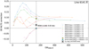 |
Fig. B.1 Interpolation of 3D NLTE corrections of the line at λ6141 Å for the star uRGB-2. Circles represent values listed in the original tables, the parameters of which are given in the legends. Lines, coloured the same as the circles, are linear interpolations. The crosses represent values interpolated in Teff and log g. The black cross displays the interpolated value in Teff, log g, and [Fe/H]. The REW of the line and the 3D NLTE corrections are noted in the plot. |
We obtain a minor value of +0.03 dex from the lines 6141 and 6496 Å, which support our A(Ba) determinations under 1D LTE and their corresponding  . Corrections towards lower A(Ba) are suitable for stars with both [Fe/H] = −1 dex and weaker Ba lines (e.g. EW ~ 100 or REW 4.9); see Fig. B.1.
Appendix C The differences between TO-1 and TO-2
Figure C.1 shows line fits of all TO stars. From top to bottom, each row shows the lines 5853, 6141, and 6496 Å, respectively. We note that the lines of the TO-2 star are visibly smaller than those of the other stars; REW are annotated in the plots. Since the atmospheric parameters of these stars are very similar, the line strengths of TO-2 support its relative lower abundance. The low Ba abundance of the TO-2 star is also noted by Schiappacasse-Ulloa & Lucatello (2023).
Appendix D Detailed estimate on the Ba isotopic ratio uncertainties
First we examine σBa-iso. In Fig. D.1 we provide examples of the degeneracy of barium abundance with isotopic ratios for the resolution of our spectra. We test 100, 75, and 0% s-process contributions letting A(Ba) vary freely. For TO-1, we obtain A(Ba) values compatible with that determined from subordinate lines (1.15 ± 0.03 dex) for 100 and 75% s-process profiles (top left and middle panels); whereas the abundance from the r-process (top right panel) is certainly too low. For TO-2, only the A(Ba) from the 0% s-process is compatible with the values determined from the subordinate lines (0.39 ± 0.02 dex). r-process profiles are wider than s-process ones due to the prominence of odd isotopes, which are split towards the line wings; see Fig. 2. For spectra of R ~ 45 000, r-process profiles appear deeper than s-process ones (compare the cyan and red profiles in Fig. D.1, for example), thus these yield lower abundances when fitted to observational lines. These results indicate that an abundance variation of about +0.35 dex10 is able to change the diagnosis of isotopic ratio from r- to s-process (i.e. from 0 to 100% s-process). Assuming a linear relation, a variation of ±1% of s-process contribution is associated to ±0.0035 dex; therefore σBa-iso (in percentage) is given by σsn between 0.0035. Since our estimate of Σiso include the effects of Teff and υmic errors separately, we determine σBa-iso only using the dispersion of the abundances of the subordinate lines (i.e. σsn).
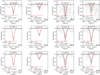 |
Fig. C.1 Fits of the subordinate lines of the TO stars. Left and right panels show spectra of the TO-1, TO-2, TO-3, and TO-4 stars, respectively; these share the same scales. Red lines represent synthetic line profiles under LTE, its associated abundance are noted in red with errors between brackets. Shade areas represent fitting errors related to the noise, which are noted within brackets. |
We estimate σT-iso using a synthetic grid of the line 4934 Å with parameters representing the defined evolutionary stages (TO, SG, bRGB, ocRGB, and uRGB) and assuming s-process contribution of 50%. We varied Teff of the spectra of simulated stars by ±50 K with respect to the values of the grid. We obtain the percentage variations in Table 6. σt-iso affect more seriously the isotope ratios diagnosis than any other source. As the quantities in the table show, a Teff change as low as 50 K may change the contribution of the s-process by up to 30%. Considering that typical Teff uncertainties of metal-poor stars in spectroscopic surveys are of ~ 100 K, and that custom spectroscopic methods are prone to bias Teff by more than 100 K in metal-poor stars (e.g. Figs. 2, 11, and A.5 in Giribaldi & Smiljanic 2023; Giribaldi et al. 2023, 2025, respectively), the accurate determination of Teff becomes paramount in the diagnosis of isotopic ratios.
Regarding σv-iso, an estimate of its impact in the s-process contribution percentage is obtained via the impact of A(Ba). In Fig. D.2 we show the change of A(Ba) with υmic in the line 4934 Å for all the evolutionary stages, where the abundance of the cluster is set to be A(Ba) = 1.15 ± 0.08 dex (gray shade). Using the fraction defined above for σsn, we can make the division of the A(Ba) error (±0.08 dex) between 0.0035 to obtain a 23% error of the s-process contribution. Now, the microturbulence ranges in Fig. D.2 (horizontal axis) that correspond to this range of A(Ba) = 1.15 ± 0.08 dex are represented in Fig. 8 by the red error bars. The mean values of these errors are 0.1, 0.1, 0.2, and 0.2 km s −1 in the uRGB, ocRGB, bRGB, and SG stages, respectively. Therefore, these υmic errors are related to an error of 23% error s-process determination. Table 6 lists the percentage error related to υmic ± 0.10 km s −1 for every evolutionary stage. The percentage errors in the TO stars were determined manually by changing vmic during the isotopic ratio determination.
The resonance line at 4934 Å has often been avoided to derive isotopic ratios in the literature (e.g. Mashonkina & Zhao 2006; Gallagher et al. 2020) because it is blended with a small Fe I line We provide estimates of the effects of the [Fe/H] errors on Σiso to demonstrate that the contribution of the Fe line blending to the error budget is minor. The errors are computed similarly to those calculated for Teff. We changed the true [Fe/H] by ±0.10 dex, and we obtained the values in Table 6.
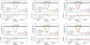 |
Fig. D.1 Fits of the resonance line 4934 Å of the TO stars. Top and bottom panels correspond to the TO-1 and TO-2 star, respectively. Left, middle, and right panels show fits of 100, 75, and 0% s-process profiles, respectively. For comparison, every panel shows line profiles of s- (cyan dashed line) and r-process (red dashed line) with an abundance equal to that determined by the fits (characters in red). Residuals of the fits are shown below the main plots. Fitting errors related to the noise are covered by shades. |
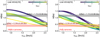 |
Fig. D.2 Similar to Fig. 5 for the line at 4934 Å. From left to right panels, the isotopic ratios assumed for the synthesis correspond to 100 and 0% s-process contributions. Gray and pink shades cover A(Ba) of the TO-1 and TO-2 stars, respectively, including dispersions. The dispersions of ±0.08 dex are σsn and σT added in quadrature (see Table 3). |
Appendix E Checking the presence of stellar activity
Our study includes two TO dwarf stars, which are at least 10 Gyr old according to isochrone fit of the cluster’s sequence (see Fig. 4). At this age, no Ba excess is observed in dwarf field stars (e.g. Fig. 1 in Reddy & Lambert 2017). Therefore, it is unlikely that the Ba abundances in our TO stars are influenced by the physical phenomena underlying the barium puzzle (see, e.g. D’Orazi et al. 2009; Baratella et al. 2020), and thus they can be considered reliable. Regarding our RGB and SG stars, no measurements of Ba excess in similarly old stars at these evolutionary stages are available in the literature.
To confirm the absence of magnetic activity, we examinated the spectra of our sample stars searching for the He I D3 line at λ5875.62 Å, which is a chromospheric activity indicator; we show four spectra with the highest S/N in our sample in Fig. E.1. Not even the spectrum of the highest quality (star uRGB-1 with S/N = 191 at λ5875.62 Å) shows any trace of the line. However, we can estimate the highest limit of its activity assuming that a line is masked by the spectral noise. In this case, the line depth must be of 1% at most, considering a 2σ detection; roughly, the line would be of EW ≲ 2 mÅ. Assuming that the relation11 between the He I D3 index and the Ca II H and K index log R'Hk of Reddy & Lambert (2017) is suitable for metal-poor RGB stars, EW = 2 mÅ is equivalent to log R'Hk = −5. This number indicates a base level of negligible chromospheric activity and null Ba excess (Figs. 9 and 10 in the paper), thus our RGB and SG stars should not present atypical enhancements due to chromospheric activity.
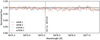 |
Fig. E.1 Spectra of our uRGB and ocRGB stars around the wavelength λ5875.62 Å of the He I D3 line. The wavelength where the He I D3 line is indicated by the dashed line. |
Appendix F The role of atomic diffusion
In the literature, there has been some controversy on whether element abundance offsets between TO and RGB stars are proofs of atomic diffusion (see e.g. Korn 2008). This is a topic of high relevance in fundamental physics because it could solve the cosmic lithium problem (e.g. Spite & Spite 1982; Ryan et al. 1999; Fields 2011). Since our method is different to those used by diverse authors assessing the presence of atomic diffusion (Korn et al. 2006, 2007; Lind et al. 2008; Nordlander et al. 2012; Gruyters et al. 2013, 2014; Souto et al. 2018, 2019, among others) our results may be considered an independent test for the presence of diffusion in this cluster. The argument against the diffusion hypothesis supports that the abundance offsets between the TO and the RGB are artifacts produced by spectroscopic methods.
Figure F.1 shows the trends of [Fe/H] as function of Teff and the evolutionary state, under LTE and NLTE. Although there is an offset between the two sets of determinations, both show a systematic increase of [Fe/H] in the stars out of the TO. The trend of our chosen NLTE [Fe/H] shows an increase of +0.25 dex at bRGB with respect to the TO (the TO-2 star was neglected in the LOWESS fit). Compared with Gruyters et al. (2013), who analyse the same cluster, under 1D LTE, we observe a similar diffusion effect. Under 1D NLTE, we measure an effect that is approximately +0.15 dex higher than the observed [Fe/H], and +0.10 to +0.15 dex above theoretical predictions.
In the following, we investigate whether the [Fe/H] offset between the TO and RGB stars shown in Fig. F.1 may result from our spectroscopic analysis method. First, we applied the Fe II 3D NLTE corrections from Amarsi et al. (2016) to the 1D NLTE [Fe/H] values in Fig. F.1, obtaining an increase by +0.10 dex for both TO and RGB stars. Therefore, 3D NLTE adjustments cannot reconcile the observed [Fe/H] offset. We also tested the Teff scale, as the impact of log g changes in [Fe/H] are usually negligible12. Assuming the 1D NLTE framework, reconciling the [Fe/H] offset would require adjusting the TO stars’ Teff upward by roughly 250 K, or lowering the RGB stars’ Teff by a similar amount. Under 3D NLTE Hα modelling (Giribaldi et al. 2021, 2023), the Teff scale shifts by at most 75 K. Therefore, Hα-based 3D NLTE Teff determinations cannot account for the 250 K adjustment required.
Finally, in Giribaldi et al. (2021), we have shown that residual instrument patterns in UVES spectra may affect Hα Teff, however no deviation larger than 80 K was observed (Fig. 6 in the paper). Therefore, given current evidence, the diffusion pattern shown in the figure is most likely authentic.
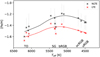 |
Fig. F.1 Metallicity as function of Teff. Red and black crosses represent NLTE and LTE determinations, respectively. The errors of NLTE values are represented by the black bars. Red and black curves are corresponding LOWESS regressions (TO-2 neglected). Evolutionary states are noted in the plot. |
Appendix G Extra Figures
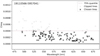 |
Fig. G.1 χ2 of the Gaussian fits of Fe lines as function of the wavelength. This plot corresponds to the star bRGB-1 or 19110566-5957041. Dark crosses represent accepted lines, whereas gray crosses represent clipped lines. The dashed red line separates the 75% quantile. |
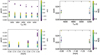 |
Fig. G.2 A(Ba) grid of offsets induced by Teff (+40 K) offsets when derived from the line 6141 Å. The left and right columns display the grids of TO and RGB stars, respectively. The horizontal line represents no offset. "X" represents the element, Ba in this case. |
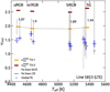 |
Fig. G.3 Same as left panel in Fig. 6, but its values are from A(Ba) = 0.89 dex, instead of A(Ba) = 1.13 dex. |
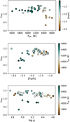 |
Fig. G.4 Microturbulence of the TITANS I dwarf sample. Values are plotted as functions of the atmospheric parameters following the colour-coding of the pallets. |
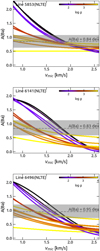 |
Fig. G.5 Similar to Fig. 5, but under NLTE. A(Ba) was derived using the Ba model atom in Gerber et al. (2023) and the departure coefficients of (Gallagher et al. 2020). |
References
- Amarsi, A. M., Lind, K., Asplund, M., Barklem, P. S., & Collet, R. 2016, MNRAS, 463, 1518 [NASA ADS] [CrossRef] [Google Scholar]
- Amarsi, A. M., Nordlander, T., Barklem, P. S., et al. 2018, A&A, 615, A139 [NASA ADS] [CrossRef] [EDP Sciences] [Google Scholar]
- Aoki, W., Beers, T. C., Honda, S., et al. 2025, PASJ, 77, 502 [Google Scholar]
- Asplund, M., Nordlund, Å., Trampedach, R., & Stein, R. F. 2000, A&A, 359, 743 [NASA ADS] [Google Scholar]
- Astropy Collaboration (Price-Whelan, A. M., et al.) 2018, AJ, 156, 123 [Google Scholar]
- Baratella, M., D’Orazi, V., Carraro, G., et al. 2020, A&A, 634, A34 [NASA ADS] [CrossRef] [EDP Sciences] [Google Scholar]
- Baratella, M., D’Orazi, V., Sheminova, V., et al. 2021, A&A, 653, A67 [NASA ADS] [CrossRef] [EDP Sciences] [Google Scholar]
- Beers, T. C., & Christlieb, N. 2005, ARA&A, 43, 531 [NASA ADS] [CrossRef] [Google Scholar]
- Bergemann, M., Lind, K., Collet, R., Magic, Z., & Asplund, M. 2012, MNRAS, 427, 27 [Google Scholar]
- Blackwell, D. E., Shallis, M. J., & Selby, M. J. 1979, MNRAS, 188, 847 [NASA ADS] [CrossRef] [Google Scholar]
- Bressan, A., Marigo, P., Girardi, L., et al. 2012, MNRAS, 427, 127 [NASA ADS] [CrossRef] [Google Scholar]
- Casagrande, L., Lin, J., Rains, A. D., et al. 2021, MNRAS, 507, 2684 [NASA ADS] [CrossRef] [Google Scholar]
- Cescutti, G., Morossi, C., Franchini, M., et al. 2021, A&A, 654, A164 [NASA ADS] [CrossRef] [EDP Sciences] [Google Scholar]
- Choplin, A., Siess, L., & Goriely, S. 2021, A&A, 648, A119 [NASA ADS] [CrossRef] [EDP Sciences] [Google Scholar]
- Choplin, A., Siess, L., & Goriely, S. 2022, A&A, 667, A155 [NASA ADS] [CrossRef] [EDP Sciences] [Google Scholar]
- Choplin, A., Siess, L., Goriely, S., & Martinet, S. 2024, A&A, 684, A206 [NASA ADS] [CrossRef] [EDP Sciences] [Google Scholar]
- Cowan, J. J., & Rose, W. K. 1977, ApJ, 212, 149 [Google Scholar]
- da Silva, A. R., & Smiljanic, R. 2025, A&A, 696, A122 [NASA ADS] [CrossRef] [EDP Sciences] [Google Scholar]
- De Munshi, D., Dutta, T., Rebhi, R., & Mukherjee, M. 2015, Phys. Rev. A, 91, 040501 [Google Scholar]
- Denissenkov, P. A., Herwig, F., Perdikakis, G., & Schatz, H. 2021, MNRAS, 503, 3913 [NASA ADS] [CrossRef] [Google Scholar]
- D’Orazi, V., Biazzo, K., Desidera, S., et al. 2012, MNRAS, 423, 2789 [Google Scholar]
- D’Orazi, V., Magrini, L., Randich, S., et al. 2009, ApJ, 693, L31 [Google Scholar]
- Dutra-Ferreira, L., Pasquini, L., Smiljanic, R., Porto de Mello, G. F., & Steffen, M. 2016, A&A, 585, A75 [NASA ADS] [CrossRef] [EDP Sciences] [Google Scholar]
- Fields, B. D. 2011, Annu. Rev. Nucl. Particle Sci., 61, 47 [Google Scholar]
- Fitzpatrick, E. L. 1999, PASP, 111, 63 [Google Scholar]
- Gaia Collaboration (Vallenari, A., et al.) 2023, A&A, 674, A1 [NASA ADS] [CrossRef] [EDP Sciences] [Google Scholar]
- Gallagher, A. J., Bergemann, M., Collet, R., et al. 2020, A&A, 634, A55 [NASA ADS] [CrossRef] [EDP Sciences] [Google Scholar]
- Gerber, J. M., Magg, E., Plez, B., et al. 2023, A&A, 669, A43 [NASA ADS] [CrossRef] [EDP Sciences] [Google Scholar]
- Gilmore, G., Randich, S., Worley, C. C., et al. 2022, A&A, 666, A120 [NASA ADS] [CrossRef] [EDP Sciences] [Google Scholar]
- Giribaldi, R. E., & Smiljanic, R. 2023, A&A, 673, A18 [NASA ADS] [CrossRef] [EDP Sciences] [Google Scholar]
- Giribaldi, R. E., Ubaldo-Melo, M. L., Porto de Mello, G. F., et al. 2019, A&A, 624, A10 [NASA ADS] [CrossRef] [EDP Sciences] [Google Scholar]
- Giribaldi, R. E., da Silva, A. R., Smiljanic, R., & Cornejo Espinoza, D. 2021, A&A, 650, A194 [NASA ADS] [CrossRef] [EDP Sciences] [Google Scholar]
- Giribaldi, R. E., Van Eck, S., Merle, T., et al. 2023, A&A, 679, A110 [NASA ADS] [CrossRef] [EDP Sciences] [Google Scholar]
- Giribaldi, R. E., Magrini, L., Rossi, M., et al. 2025, A&A, 698, A11 [NASA ADS] [CrossRef] [EDP Sciences] [Google Scholar]
- Goriely, S. 1999, A&A, 342, 881 [NASA ADS] [Google Scholar]
- Goriely, S., & Siess, L. 2018, A&A, 609, A29 [NASA ADS] [CrossRef] [EDP Sciences] [Google Scholar]
- Goriely, S., Siess, L., & Choplin, A. 2021, A&A, 654, A129 [NASA ADS] [CrossRef] [EDP Sciences] [Google Scholar]
- Gratton, R. G., Bonifacio, P., Bragaglia, A., et al. 2001, A&A, 369, 87 [NASA ADS] [CrossRef] [EDP Sciences] [Google Scholar]
- Grevesse, N., Asplund, M., & Sauval, A. J. 2007, Space Sci. Rev., 130, 105 [Google Scholar]
- Gruyters, P., Korn, A. J., Richard, O., et al. 2013, A&A, 555, A31 [NASA ADS] [CrossRef] [EDP Sciences] [Google Scholar]
- Gruyters, P., Nordlander, T., & Korn, A. J. 2014, A&A, 567, A72 [NASA ADS] [CrossRef] [EDP Sciences] [Google Scholar]
- Gull, M., Frebel, A., Cain, M. G., et al. 2018, ApJ, 862, 174 [Google Scholar]
- Gurtovenko, E. A., & Sheminova, V. A. 2015, arXiv e-prints [arXiv:1505.00975] [Google Scholar]
- Gustafsson, B., Edvardsson, B., Eriksson, K., et al. 2008, A&A, 486, 951 [NASA ADS] [CrossRef] [EDP Sciences] [Google Scholar]
- Hansen, T. T., Hansen, C. J., Christlieb, N., et al. 2015, ApJ, 807, 173 [CrossRef] [Google Scholar]
- Hansen, T. T., Andersen, J., Nordström, B., et al. 2016, A&A, 588, A3 [NASA ADS] [CrossRef] [EDP Sciences] [Google Scholar]
- Hansen, T. T., Holmbeck, E. M., Beers, T. C., et al. 2018, ApJ, 858, 92 [Google Scholar]
- Heiter, U., Lind, K., Bergemann, M., et al. 2021, A&A, 645, A106 [EDP Sciences] [Google Scholar]
- Hourihane, A., François, P., Worley, C. C., et al. 2023, A&A, 676, A129 [NASA ADS] [CrossRef] [EDP Sciences] [Google Scholar]
- Itano, W. M. 2006, Phys. Rev. A, 73, 022510 [Google Scholar]
- Jackson, R. J., Jeffries, R. D., Wright, N. J., et al. 2022, MNRAS, 509, 1664 [Google Scholar]
- Jofré, P., Heiter, U., Soubiran, C., et al. 2014, A&A, 564, A133 [NASA ADS] [CrossRef] [EDP Sciences] [Google Scholar]
- Jonsell, K., Barklem, P. S., Gustafsson, B., et al. 2006, A&A, 451, 651 [NASA ADS] [CrossRef] [EDP Sciences] [Google Scholar]
- Korn, A. 2008, Mem. Soc. Astron. Italiana, 79, 495 [Google Scholar]
- Korn, A. J., Grundahl, F., Richard, O., et al. 2006, Nature, 442, 657 [Google Scholar]
- Korn, A. J., Grundahl, F., Richard, O., et al. 2007, ApJ, 671, 402 [NASA ADS] [CrossRef] [Google Scholar]
- Lind, K., Korn, A. J., Barklem, P. S., & Grundahl, F. 2008, A&A, 490, 777 [NASA ADS] [CrossRef] [EDP Sciences] [Google Scholar]
- LOWESS 2021, https://doi.org/10.5281/zenodo.4642896 [Google Scholar]
- Magrini, L., Bensby, T., Brucalassi, A., et al. 2023, arXiv e-prints [arXiv:2312.08270] [Google Scholar]
- Martinet, S., Choplin, A., Goriely, S., & Siess, L. 2024, A&A, 684, A8 [NASA ADS] [CrossRef] [EDP Sciences] [Google Scholar]
- Mashonkina, L., & Zhao, G. 2006, A&A, 456, 313 [NASA ADS] [CrossRef] [EDP Sciences] [Google Scholar]
- Mashonkina, L., Gehren, T., & Bikmaev, I. 1999, A&A, 343, 519 [NASA ADS] [Google Scholar]
- Meléndez, J., & Barbuy, B. 2009, A&A, 497, 611 [NASA ADS] [CrossRef] [EDP Sciences] [Google Scholar]
- Meng, X. Y., Cui, W. Y., Shi, J. R., et al. 2016, A&A, 593, A62 [EDP Sciences] [Google Scholar]
- Nordlander, T., Korn, A. J., Richard, O., & Lind, K. 2012, ApJ, 753, 48 [NASA ADS] [CrossRef] [Google Scholar]
- Nordlander, T., Gruyters, P., Richard, O., & Korn, A. J. 2024, MNRAS, 527, 12120 [Google Scholar]
- Pancino, E., Lardo, C., Altavilla, G., et al. 2017, A&A, 598, A5 [NASA ADS] [CrossRef] [EDP Sciences] [Google Scholar]
- Randich, S., Gilmore, G., Magrini, L., et al. 2022, A&A, 666, A121 [NASA ADS] [CrossRef] [EDP Sciences] [Google Scholar]
- Reddy, A. B. S., & Lambert, D. L. 2017, ApJ, 845, 151 [Google Scholar]
- Ryan, S. G., Norris, J. E., & Beers, T. C. 1999, ApJ, 523, 654 [CrossRef] [Google Scholar]
- Sbordone, L., Hansen, C. J., Monaco, L., et al. 2020, A&A, 641, A135 [EDP Sciences] [Google Scholar]
- Schiappacasse-Ulloa, J., & Lucatello, S. 2023, MNRAS, 520, 5938 [NASA ADS] [CrossRef] [Google Scholar]
- Schiappacasse-Ulloa, J., Lucatello, S., Rain, M. J., & Pietrinferni, A. 2022, MNRAS, 511, 231 [NASA ADS] [CrossRef] [Google Scholar]
- Schiappacasse-Ulloa, J., Magrini, L., Lucatello, S., et al. 2025, A&A, 699, A41 [NASA ADS] [CrossRef] [EDP Sciences] [Google Scholar]
- Semenova, E., Bergemann, M., Deal, M., et al. 2020, A&A, 643, A164 [NASA ADS] [CrossRef] [EDP Sciences] [Google Scholar]
- Silverans, R. E., Borghs, G., de Bisschop, P., & van Hove, M. 1986, Phys. Rev. A, 33, 2117 [Google Scholar]
- Sitnova, T. M., Lombardo, L., Mashonkina, L. I., et al. 2025, A&A, 699, A262 [NASA ADS] [CrossRef] [EDP Sciences] [Google Scholar]
- Souto, D., Cunha, K., Smith, V. V., et al. 2018, ApJ, 857, 14 [NASA ADS] [CrossRef] [Google Scholar]
- Souto, D., Allende Prieto, C., Cunha, K., et al. 2019, ApJ, 874, 97 [NASA ADS] [CrossRef] [Google Scholar]
- Spite, M., & Spite, F. 1982, Nature, 297, 483 [NASA ADS] [CrossRef] [Google Scholar]
- Steffen, M., Caffau, E., & Ludwig, H. G. 2013, Mem. Soc. Astron. Ital. Suppl., 24, 37 [Google Scholar]
- Steffen, M., Ludwig, H.-G., Wedemeyer-Böhm, S., & Gallagher, A. 2023, Linfor3D User Manual [Google Scholar]
- Takeda, Y. 2022, Sol. Phys., 297, 4 [NASA ADS] [CrossRef] [Google Scholar]
- Trapp, S., Marx, G., Tommaseo, G., et al. 2000, Hyperfine Interact., 127, 57 [Google Scholar]
- Vasiliev, E., & Baumgardt, H. 2021, MNRAS, 505, 5978 [NASA ADS] [CrossRef] [Google Scholar]
- Villemoes, P., Arnesen, A., Heijkenskjold, F., & Wannstrom, A. 1993, J. Phys. B At. Mol. Phys., 26, 4289 [NASA ADS] [CrossRef] [Google Scholar]
- Wen, F., Cui, W., Tian, M., et al. 2022, Universe, 8, 596 [Google Scholar]
Here, metallicity is determined using the element Fe as a proxy. We use the iron to hydrogen fraction relative to the Sun in logarithmic scale as follows: [A/B] =  , where N denotes the number abundance of a given element.
log(EW/λ), where EW is the equivalent width in Å and λ is the wavelength in Å.
 , where N(Ba) and N(H) are the number densities (abundances by number) of barium and hydrogen, respectively.
Locally Weighted Scatterplot Smoothing (LOWESS) regressions are applied by the Python moepy package LOWESS (2021) available at https://ayrtonb.github.io/Merit-Order-Effect/, using the parameter frac=0.55.
Similar values are found in both dwarfs and giants.
We use Equation 1 of the paper.
The highest impact of log g is the SG branch, where changes of ±0.3 dex induce [Fe/H] ∓0.1 dex, approximately.
All Tables
All Figures
|
Fig. 1 Theoretical curves of growth for the two Ba resonance lines. Equivalent widths (EW) were computed in spectra synthesised by MARCS 1D atmosphere models adopting the atmospheric parameters Teff = 5540 K, log g = 2.45, [Fe/H] = −2.00 dex, and υmic = 1.5 km s−1. The barium abundance in the horizontal axis is neglected on purpose, as the scale depends on the abundance itself and the stellar parameters. The location of our stars is indicated by the red circles, where they are designated according to their evolutionary state as follows: turn-off (TO), subgiant (SG), base of the red giant branch (bRGB), over the clump RGB (ocRGB), and upper RGB (uRGB). |
| In the text | |
|
Fig. 2 Synthetic profiles of the line at λ4934 Å. The synthesis was made with the Turbospectrum code (Gerber et al. 2023) and MARCS models. See details in Sect. 5.2. The atmospheric parameters for the synthesis are similar to those of the star GES J19102677-6003089 (TO-1) in Table 2. The spectrum has resolution R = λ/∆λ = 493 000 and infinite S/N. The solid line (r-process), dashed line (s-process), and blue shade (i-process) profiles are synthesised with the isotopic ratios in Table 5. |
| In the text | |
|
Fig. 3 Colour-magnitude diagram of NGC 6752. Grey and red symbols represent stars in the cluster field and the sample analysed in the present work, respectively. Photometry for both samples was taken from Gaia eDR3. An isochrone of 12 Gyr is overplotted as a reference. |
| In the text | |
|
Fig. 4 Kiel diagram of the program stars. Red circles display Teff and log gNLTE. Gray circles display log gLTE. Quantities are listed in Table 2. |
| In the text | |
|
Fig. 5 LTE barium abundance as function of υmic for the subordinate lines 5853, 6141, and 6496 Å. Each trend is related to one star and is colour-coded according to log g. Shades enclose the most probable ranges of A(Ba) of the TO-1 and TO-2 stars; see main text. Dashed gray and red lines indicate the mean A(Ba) in the shades for each star, respectively. |
| In the text | |
|
Fig. 6 Microturbulence as function of Teff for the stars in Table 1. Panels descriptions, from left to right, are as follows. Quantities derived from the subordinate lines at λ5853, 6141, and 6496 Å, respectively. TO stars are excluded on purpose. Vertical bars represent υmic ranges computed by the intersections of the trends with the shades in Fig. 5. Orange dashes are medians of contiguous bars, which correspond to stars in the stages indicated on the top; these values are defined as |
| In the text | |
|
Fig. 7 Microturbulence as function of Teff for the line 4934 Å. Left and centre panels shows quantities derived assuming 100 and 0% s-process contributions, respectively. A(Ba) = 1.15 ± 0.08 dex of the TO-1 star is assumed in both cases. Right panel shows quantities derived assuming the A(Ba) = 0.39 ± 0.08 dex and full r-process contribution of the TO-2 star. Black bars represent the microturbulence ranges required to fit observational lines with synthetic ones. Red dashes are the medians of the bars in the stages indicated on the top. The red and blue dotted lines are linear regressions of the red and blue dashes, respectively. |
| In the text | |
|
Fig. 8 Microturbulence as function of EW and REW for the Ba resonance line at λ4934 Å. Microturbulence values determined from diverse methods are represented according to the legends. The solid black line is the polynomial regression of |
| In the text | |
|
Fig. 9 Fits of the 4934 Å Ba resonance line. The stars to which each plot corresponds are indicated in the plots. The observational profiles are represented by the black lines. Synthetic profiles are represented by coloured lines. The synthetic profiles most compatible with the observational ones are represented by the thick olive lines; their s-process contributions are noted along with the errors related to the noise. Synthetic profiles related to s- and r-processes are represented by the dotted or dashed green lines according to the legends. A synthetic spectra without barium are represented by the dotted red lines. The probability for a given process to dominate the line profile shape is given by the χ2 in the inner plot. The shades in the inner plots cover errors of the s-process contribution. Residual plots are shown at the bottom panel, where the shades represent the areas covered by the fitting errors. |
| In the text | |
|
Fig. B.1 Interpolation of 3D NLTE corrections of the line at λ6141 Å for the star uRGB-2. Circles represent values listed in the original tables, the parameters of which are given in the legends. Lines, coloured the same as the circles, are linear interpolations. The crosses represent values interpolated in Teff and log g. The black cross displays the interpolated value in Teff, log g, and [Fe/H]. The REW of the line and the 3D NLTE corrections are noted in the plot. |
| In the text | |
|
Fig. C.1 Fits of the subordinate lines of the TO stars. Left and right panels show spectra of the TO-1, TO-2, TO-3, and TO-4 stars, respectively; these share the same scales. Red lines represent synthetic line profiles under LTE, its associated abundance are noted in red with errors between brackets. Shade areas represent fitting errors related to the noise, which are noted within brackets. |
| In the text | |
|
Fig. D.1 Fits of the resonance line 4934 Å of the TO stars. Top and bottom panels correspond to the TO-1 and TO-2 star, respectively. Left, middle, and right panels show fits of 100, 75, and 0% s-process profiles, respectively. For comparison, every panel shows line profiles of s- (cyan dashed line) and r-process (red dashed line) with an abundance equal to that determined by the fits (characters in red). Residuals of the fits are shown below the main plots. Fitting errors related to the noise are covered by shades. |
| In the text | |
|
Fig. D.2 Similar to Fig. 5 for the line at 4934 Å. From left to right panels, the isotopic ratios assumed for the synthesis correspond to 100 and 0% s-process contributions. Gray and pink shades cover A(Ba) of the TO-1 and TO-2 stars, respectively, including dispersions. The dispersions of ±0.08 dex are σsn and σT added in quadrature (see Table 3). |
| In the text | |
|
Fig. E.1 Spectra of our uRGB and ocRGB stars around the wavelength λ5875.62 Å of the He I D3 line. The wavelength where the He I D3 line is indicated by the dashed line. |
| In the text | |
|
Fig. F.1 Metallicity as function of Teff. Red and black crosses represent NLTE and LTE determinations, respectively. The errors of NLTE values are represented by the black bars. Red and black curves are corresponding LOWESS regressions (TO-2 neglected). Evolutionary states are noted in the plot. |
| In the text | |
|
Fig. G.1 χ2 of the Gaussian fits of Fe lines as function of the wavelength. This plot corresponds to the star bRGB-1 or 19110566-5957041. Dark crosses represent accepted lines, whereas gray crosses represent clipped lines. The dashed red line separates the 75% quantile. |
| In the text | |
|
Fig. G.2 A(Ba) grid of offsets induced by Teff (+40 K) offsets when derived from the line 6141 Å. The left and right columns display the grids of TO and RGB stars, respectively. The horizontal line represents no offset. "X" represents the element, Ba in this case. |
| In the text | |
|
Fig. G.3 Same as left panel in Fig. 6, but its values are from A(Ba) = 0.89 dex, instead of A(Ba) = 1.13 dex. |
| In the text | |
|
Fig. G.4 Microturbulence of the TITANS I dwarf sample. Values are plotted as functions of the atmospheric parameters following the colour-coding of the pallets. |
| In the text | |
|
Fig. G.5 Similar to Fig. 5, but under NLTE. A(Ba) was derived using the Ba model atom in Gerber et al. (2023) and the departure coefficients of (Gallagher et al. 2020). |
| In the text | |
Current usage metrics show cumulative count of Article Views (full-text article views including HTML views, PDF and ePub downloads, according to the available data) and Abstracts Views on Vision4Press platform.
Data correspond to usage on the plateform after 2015. The current usage metrics is available 48-96 hours after online publication and is updated daily on week days.
Initial download of the metrics may take a while.