| Issue |
A&A
Volume 703, November 2025
|
|
|---|---|---|
| Article Number | A51 | |
| Number of page(s) | 16 | |
| Section | Astrophysical processes | |
| DOI | https://doi.org/10.1051/0004-6361/202453593 | |
| Published online | 06 November 2025 | |
Cosmic ray transport and acceleration in an evolving shock landscape
1
Ruhr-Universität Bochum, Fakultät für Physik und Astronomie, Institut für Theoretische Physik IV, Universitätsstraße 150 44780 Bochum, Germany
2
Ruhr Astroparticle and Plasma Physics Center (RAPP Center), Bochum, Germany
3
Department of Astronomy, University of Wisconsin–Madison, 475 N. Charter Street, Madison, WI 53706, USA
4
Department of Physics, University of Wisconsin–Madison, 150 University Avenue, Madison, WI 53706-1390, USA
5
Chalmers University of Technology, Department of Space, Earth and Environment, 412 96 Gothenburg, Sweden
⋆ Corresponding author: This email address is being protected from spambots. You need JavaScript enabled to view it.
Received:
23
December
2024
Accepted:
4
September
2025
Abstract
Context. Cosmic rays are detected from 109 eV up to 1020 eV, with two distinct changes in the spectrum at ∼1015 eV and at 1018.5 eV. Below the first break (i.e., cosmic-ray knee), sources of acceleration are believed to be located in the Milky Way. Above the second break (i.e., cosmic-ray ankle) the population is expected to be extragalactic. In between the two, there is a need to take into account a third population of sources with the capacity to accelerate particles to extreme energies. In addition to a Galactic wind and its termination shock, large-scale shock structures in the Galactic halo have been proposed to fill the gap.
Aims. In this paper, we investigate CR transport in a time-dependent landscape of shocks in the Galactic halo. These shocks could result from local outbursts, for instance, star-forming regions and superbubbles. CRs re-accelerated at such shocks can reach energies above the knee. Since the shocks are closer to the Galaxy than a termination shock and CRs escape downstream, they can propagate back more easily. With such outbursts happening frequently, shocks are bound to interact. This interaction could adjust the CR spectrum, particularly for the particles that are able to be accelerated at two shocks simultaneously.
Methods. The transport and acceleration of CRs at the shock is modeled by stochastic differential equations (SDEs) within the public CR propagation framework CRPropa. We developed extensions for time-dependent wind profiles and, for the first time, we connected the code to hydrodynamic simulations, which were run with the public Athena++ code.
Results. We find that depending on the concrete realization of the diffusion tensor, a significant fraction of CRs can make it back to the Galaxy. These could contribute to the observed spectrum around and above the CR knee (E ≳ 10 PeV). In contrast to simplified models, a simple power law does not describe the energy spectra well. Instead, for single shocks, we find a flat spectrum (E−2) at low energies, which steepens gradually until it reaches an exponential decline. When shocks collide, the energy spectra transiently become harder than E−2 at high energies.
Key words: acceleration of particles / diffusion / hydrodynamics / plasmas / shock waves / Galaxy: halo
© The Authors 2025
 Open Access article, published by EDP Sciences, under the terms of the Creative Commons Attribution License (https://creativecommons.org/licenses/by/4.0), which permits unrestricted use, distribution, and reproduction in any medium, provided the original work is properly cited.
This article is published in open access under the Subscribe to Open model. This email address is being protected from spambots. You need JavaScript enabled to view it. to support open access publication.
1. Introduction
Cosmic rays (CRs) have been studied for decades, with their spectrum and composition being constrained over several orders of magnitude in energy; however, their origins are still unclear. While there are good arguments that CRs below the cosmic-ray knee come from local sources in the Milky Way and those above the CR ankle (1018.5 eV) originate from extragalactic sources, the mechanisms for the energy spectrum between the two kinks are still under debate Becker Tjus & Merten 2020. The transition from Galactic to extragalactic sources occurs in this energy range, thus often referred to as the transition region. Prior discussions have posited that the observed spectrum cannot simply be explained by one declining and one rising component, but that an additional source population, previously referred to as “component B”, must exist to fill the gap Hillas 2005. We note that the transition between ballistic and diffusive transport is also expected in this energy range between the knee and the ankle for the Galactic magnetic field.
It has been argued by several groups Jokipii & Morfill 1987; Thoudam et al. 2016; Bustard et al. 2017; Merten et al. 2018; Mukhopadhyay et al. 2023 that a Galactic wind termination shock (GWTS) could (re-)accelerate Galactic CRs to the transition region. Previous models often assumed a stationary wind profile (see e.g., Jokipii & Morfill 1987; Merten et al. 2018; Thoudam et al. 2016). This is a very optimistic assumption as the relevant timescales (e.g., the shock lifetime, time for the wind to reach the termination shock, and CR acceleration timescale) are on the same order of magnitude. Although CRs might be accelerated to the desired energies, it is very hard for them to propagate back into the Galaxy because the termination shock is far outside of the Galactic disk (Rshock ≳ 200 kpc). Additionally, they have to escape upstream, propagate against the wind, and experience adiabatic energy loss in the expanding wind.
In particular, for starburst galaxies, evidence for strong supersonic winds can be found López-Cobá et al. 2017; Veilleux et al. 2005. And, it is believed that CR feedback plays an important role in galaxy evolution, star formation, and driving of galactic winds. Star formation and outflows may be linked through the Parker instability: Non-thermal CR pressure (e.g., in regions of strong star formation) perturbs the magnetic field lines tangential to the Galactic plane, forming magnetic troughs that gas can flow through. This has the capacity to launch local galactic winds or fountains (see, e.g., Ruszkowski & Pfrommer 2023 and references therein).
In addition to the GWTS, many other source classes, such as microquasars (see e.g., Abaroa et al. 2024) and superbubbles (SB) Bykov & Fleishman 1992; Vieu et al. 2022a,b, have been proposed to contribute to the CR flux around and above ∼PeV energies. Furthermore, Völk & Zirakashvili 2004 suggested that CRs can be significantly accelerated in slipping interaction regions in the Galactic wind, resulting from the spiral structure of the Galaxy in a similar way to corotating interaction regions in the solar wind. Also, supernova remnants (SNRs) might be able to reach energies up to the spectral knee, if the magnetic field is significantly amplified due to non-linear feedback of the CRs themselves Bell & Lucek 2001; Bell 2004; Amato & Blasi 2009; however, it seems difficult to explain the missing flux with SNRs alone. A recent paper considers the effect of magnetic mirrors in the shock region Bell et al. 2025.
Dorfi & Breitschwerdt 2012 investigated the acceleration of CRs in an expanding Galactic wind that is driven by supernova (SN) and found considerable acceleration up to above the spectral knee. In this paper, we investigate particle acceleration at such non-stationary shocks moving out of the Galaxy. This has several advantages compared to the GWTS scenario: the shocks can be closer to the Galaxy, so that the distance re-accelerated CRs have to cover is way less than 200 kpc. In a blast wave scenario, the upstream region is outside of the shocked sphere; thus, re-accelerated CRs have to escape downstream to be observed at Earth. On the other hand, the downstream frame now moves with the shock speed away from the Galaxy. However, if the shock slows down over time, for instance, due to spherical expansion, this constraint becomes less severe. This makes the escape from the acceleration region and propagation back to the Galaxy more likely than at a GWTS. Furthermore, CRs spend less time in the expanding wind (or the wind slows itself down), which decreases adiabatic energy losses.
Local, non-stationary shock structures can result from perturbations in the Galaxy. Examples of this include strong SN or SB explosions driving outflows or large scale instabilities such as the Parker instability Habegger et al. 2023; Habegger & Zweibel 2024. While, for instance, the forward shock of an SB might have negligible speed within the Galactic disk Castor et al. 1975; Weaver et al. 1977; Vieu et al. 2022b, a shock can reach considerably high speeds when perturbations or SNs take place close to the edge of the Galaxy. The shocks run down a density gradient leading to an acceleration of the shock speed and the formation of a fountain or jetlike structure Dorfi & Breitschwerdt 2012; Dorfi et al. 2019. Therefore, we focus on the regions close to the edge of the Galaxy.
Observations of magnetized structures in the Galactic halo seem to be connected to star-forming regions in the Galactic disk Zhang et al. 2024 which could be sustained from such local outflows. Furthermore, evidence of the presence of relativistic electrons in the Galactic halo has been reported in previous studies Zhang et al. 2024, which offers a hint with respect to acceleration sites high above the Galactic disk. Electrons are not expected to propagate over large distances due to their small diffusion coefficient and short loss timescales.
In this paper, we take a closer look at such a scenario by studying CR acceleration at a spherical shock similar to the Sedov-Taylor blast wave, which is launched with the energy equivalent to tens up to hundreds of that of a typical SN and moves into a medium with a decreasing density profile. We derive acceleration times and estimates of the maximal energy reached at the shock. Furthermore, we obtained time-dependent energy spectra at the shock and the Galactic boundary from simulations. These spectra could potentially be observed at Earth.
With several of those perturbations happening frequently in the Galaxy, those structures build a shock landscape in the Galactic halo and contribute to a global wind structure Dorfi & Breitschwerdt 2012; Dorfi et al. 2019. Additionally, if several outbursts occur near each other in both space and time, they will likely interact when they expand outwards and might run into each other. In this work, we further study particle acceleration at two consecutive shocks that eventually merge. Similar considerations have been made for converging stellar winds and SNe in star-forming regions in a steady-state Bykov et al. 2013 and time-dependent way Vieu et al. 2020. Alternatively, for the interaction of shocks driven by coronal mass ejections in the solar wind Wang et al. 2017, 2019. In this work, we not only obtained the time-dependent energy spectra at the individual colliding shocks, but also at the single shock that develops after merging. The wind profile after the collision is given by the flow profile of the Sod shock tube problem Sod 1978. We further investigate the probability of re-accelerated CRs to end up diffusing back to the Galaxy.
We modeled the transport and acceleration of colliding shocks in one dimension and planar shocks were considered. While the scenario is idealized, it is a step toward understanding how the complex shock interactions, which drive the Galactic wind and the termination shock, could affect CR acceleration.
To obtain the spectral slope and model the propagation of CRs from the moving shocks back to the Galaxy, we used a modified version of the publicly available CR transport framework CRPropa (Alves Batista et al. 2022; Merten et al. 2017, hereafter M17). The transport equations of CRs were solved through stochastic differential equations (SDEs). The framework was tested and found to be well suited for studies of CR acceleration in different scenarios (Aerdker et al. 2024, hereafter A24; Merten & Aerdker 2025, hereafter MA24). Where no simple analytical description of the wind profiles was available, we used Athena++ Stone et al. 2020 for hydrodynamic simulations.
The paper is organized as follows: In Section 2 the basics of the implementation of the CRPropa based SDE solver are explained. In addition, we discuss all new extensions in detail, for instance, specialized adaptive steps and time-dependent wind profiles that have been developed to accurately model the scenarios discussed above. Furthermore, all new code parts are validated. The updated software framework is applied to the individual time-dependent spherical shocks propagating into the Galactic halo in Section 3. Section 4 includes the modeling of the two shocks and we discuss how the wind profile of the colliding shocks is constructed. The paper is concluded with a summary and discussion of the results in Section 5.
2. Transport description
To investigate the transport and acceleration of CRs in local and time-dependent structures, we used a modified version of CRPropa 3.2 (MA25). The transport equation is solved by rewriting it into the corresponding set of stochastic differential equations (SDEs). For details on the SDE solver that comes with the publicly available version, we refer to M17. We give a brief overview of the algorithm, but otherwise refer to M17 and MA25.
2.1. From transport equations to SDEs
The transport of CRs is modeled by the partial differential equation
 (1)
(1)
which describes the time evolution of the isotropic part of the distribution function f(x, p, t) with respect to advection u(x, t), diffusion, given by a spatial diffusion tensor  , adiabatic cooling and heating through the ∇ ⋅ u term, and sources and sinks, S(x, p, t). Here, momentum diffusion is not considered. Although we expect that in the turbulent Galactic outflows second-order acceleration can play a role to some extent, we focus on the energy spectrum that is produced by the moving shocks first. Future applications can take momentum diffusion into account, as described in MA25.
To rewrite Eq. (1) into a set of SDEs, it has to be transformed to a Fokker-Planck equation (MA25). The easiest way to do this is to consider the number density 𝒩 = fp2 instead of the distribution function,
![Mathematical equation: $$ \begin{aligned} \frac{\partial \mathcal{N} }{\partial t} = \frac{1}{2} \nabla ^2 (2\hat{\kappa }\mathcal{N} ) - \nabla \left[\left(\nabla \hat{\kappa } + \mathbf u \right) \mathcal{N} \right] - \frac{\partial }{\partial p} \left[-\frac{p}{3}(\nabla \cdot \mathbf u )\mathcal{N} \right] + \tilde{S}. \end{aligned} $$](/articles/aa/full_html/2025/11/aa53593-24/aa53593-24-eq3.gif) (2)
(2)
When rewriting Eq. (2) into SDEs, it gets split into one equation describing the spatial transport and one describing changes in momentum, which is similar to the operator splitting ansatz often used to solve the FP equation. The spatial evolution of a phase-space element or pseudo-particle is given by
 (3)
(3)
with the Wiener process, dWt, as a stochastic driver for the diffusive part. Equation (3) is solved with an Euler-Maruyama scheme with time step Δt, where the Wiener process is approximated by  . The random numbers, ηx, are drawn from a normal distribution with mean value of zero. Details are presented in M17 and MA25, for instance. For quickly changing advection, more advanced schemes such as the predictor-corrector scheme might be crucial to obtain correct results. However, in our applications, we find that the Euler-Maruyama scheme produces the expected results when the time step is chosen correctly.
The diffusion tensor,  , is usually defined in local magnetic field coordinates, where the diagonal entries describe transport parallel and perpendicular to the magnetic field line. Off-diagonal entries describe drifts due to the curvature and gradient of the magnetic field. In this work, we only consider diffusion parallel and perpendicular to the magnetic field. For details on the integration of the magnetic field line in each simulation step, we refer to M17 and MA25.
The time evolution in momentum is given by an ordinary differential equation since diffusion in momentum space, also known as second order Fermi acceleration, is not considered; in fact, it is expected to be 𝒪(vA2/c2) relative to spatial diffusion. In the diffusive or macroscopic picture, energy gain at the shock comes from the compression of the background flow. The differential equation,
 (4)
(4)
is also integrated with an Euler scheme analogous to the SDE.
Equations (3) and (4) do not describe trajectories and energy gain of physical particles but of samples of the differential number density, 𝒩 = fp2. The distribution function or number density is then obtained from an ensemble average over a large number of pseudo-particle trajectories. We refer to MA25 for details on creating histograms, for instance, of the energy spectrum and a detailed analysis of the uncertainty given by the Monte Carlo error  of the property X and the number of independent pseudo-particles N (e.g., in an energy bin Ei). Pseudo-particles, however, can depend on each other when the CandidateSplitting module is used to increase statistics at high energies.
The SDE approach is in principle independent of specific boundary conditions or source terms. Thus, as long as the phase space is sufficiently sampled in the region of interest, the solution can be re-weighted in the later analysis, for instance, when modeling a source with a different spectral slope. Also, the continuous injection of pseudo-particles can be constructed by a time integration of the solution (a summation of Green’s function, see Merten et al. 2018 for details), which saves computation time. The latter, however, is only possible when the background fields are stationary.
2.2. Updated modules
The AdvectionField modules that provide the background flow u and its divergence ∇ ⋅ u are extended to take time-dependency into account. The time-dependent advection fields will be publicly available also in the master version of CRPropa 3.21. From Eq. (4), it follows that the advection, u, has to be differentiable. This means that the shock needs to be smoothed out with a finite width (e.g., with a hyperbolic tangent). Although the shock has a finite width, compared to the (pseudo-) particles’ mean-free path, it is often treated as a discontinuity in treatments of DSA. Furthermore, the computational shock width used in the simulation does not need to be equal to the physical width of the shock and it is typically larger. The implied constraints on the shock width necessary to obtain the spectra expected at a discrete shock are discussed in Kruells & Achterberg 1994; Achterberg & Schure 2011 and validated for CRPropa in A24 and can be summarized by the following inequality,
 (5)
(5)
where Δt is the simulation time step and lsh is the shock width. The shock normal is denoted by esh.
The constraints depend on the simulation time step to ensure that the resolution is high enough for pseudo-particles to encounter the shock region. Also, from a physical perspective, the mean-free path of the particles must be larger than the shock width. For the simulation, it is sufficient that the diffusive step,  , (which is a measure for that actual stochastic integration step) is larger than the considered shock width. In that case, the mean diffusive step for the pseudo-particles can be larger than the mean-free path for a corresponding physical particle, which speeds up the simulation significantly.
The DiffusionTensor modules are extended to take Bohm diffusion in a magnetic field with varying strength into account. Changing eigenvalues of the diffusion tensor lead to an additional drift-like term in the SDE Eq. (3) (for details, we refer to, e.g., Kopp et al. 2012 and MA25).
In the following two subsections, we explain how we validated the transport and acceleration at time-dependent wind profiles by first comparing the spectra at a one-dimensional (1D) planar shock in the lab frame (where the shock is moving) and shock frame (where the shock speed is vsh = 0). We further investigated diffusive shock acceleration (DSA) at a spherical blast wave resulting from a point explosion, using the similarity solution found by Sedov and Taylor as a wind profile Kahn 1975; Sedov 1946; Taylor 1950; Isenberg 1977. The resulting spectra are compared to an analytical approximation given by Drury 1983.
2.3. 1D planar shock
We show that with the CRPropa simulation using the Euler-Maruyama scheme to integrate the SDE and ODE in Eqs. (3) and (4), we are able to obtain the same spectra at a 1D planar shock moving with vsh into an undisturbed medium, v0 = 0, and at a stationary shock with ush = 0 and upstream speed, u0 = −vsh.
The two wind profiles sketched in Fig. 1 were implemented in the modified version of CRPropa 3.2. In both cases, the shock profile is approximated by a tanh((x − xsh/lsh) function. The shock width, lsh, and time step, Δt, were chosen according to the constraints reported in the previous section. The stationary shock was set at x = 0, upstream speed is u0 = 1, and downstream speed is u1 = 1/4. Henceforth, we used computational units, for instance, [x]=kpc, [u]= 100 km/s and [t]≈10 Myr. Pseudo-particles were injected at t = 0 at x = 0 and propagated until the simulation ends at time T = 100. Assuming a continuous injection of particles, the solution was obtained by integrating over times, Ti = nΔT (see Merten et al. 2018, A24 and MA25 for details).
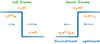 |
Fig. 1. Shock profiles in lab frame (left) and frame in which shock is stationary (right). Assuming a compression ratio q = 4 and that the preshock medium does not move (v1 = 0), the postshock speed is 3/4 of the shock speed. In the shock frame, upstream and downstream side can be specified and the downstream speed equals 1/q the upstream speed. |
In the lab frame, the shock started at x = 0 and moves with constant speed, vsh = 1. Pseudo-particles were injected at t = 0 in the range x = [0, 100]. Since the wind profile is not stationary, the solution cannot be integrated over time; thus, a factor of n more pseudo-particles were injected at t = 0. This slowed down the simulation by a factor of n, however, the uncertainty in the spectra was lower since more independent pseudo-particles are included in the simulation. For better statistics at high energies, we used the CandidateSplitting module (A24, MA25). To compensate for the low number of pseudo-particles at high energies, they were split into two copies once they crossed boundaries in energy determined by the expected power law produced by the shock. In the later analysis, they were weighted according to the number of splits.
Figure 2 shows the resulting energy distribution over space at two times T = 50, 90. The ultra-relativistic limit E ≈ pc was used. For the stationary wind, the y-axis has negative values. The horizontal pattern visible in the histogram for the stationary shock at later times, T = 90, comes from the time integration and has no associated physical effect. For an analysis on the uncertainties coming from the integration in time and the use of the splitting module, we refer to MA25.
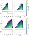 |
Fig. 2. Left: Wind profiles and space-energy histogram in the lab frame. Pseudo-particles are injected in the undisturbed medium, the shock is moving through it. Right: Stationary wind profile and space-energy histogram. Pseudo-particles are injected at the shock. For both columns, the top row shows spectra and wind profiles at T = 50 and the bottom row shows them at T = 90. |
Figure 3 shows the energy spectrum d𝒩/dE ∝ Es at the shock, x = [0, 1] for the stationary and x = [xsh, xsh + 1] moving with the shock in lab frame over time. Both the expected spectral slope s = −2 for a compression of 4 and the time evolution match very well. To reach the stationary solution over the full energy range, the simulations needs to run for a longer time.
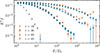 |
Fig. 3. Energy spectra at the shocks in the lab frame (moving with the shock) (blue) and in the stationary shock frame (orange). The resulting spectral slope and time evolution are the same. Error bars are obtained from the Monte Carlo error in each bin and proportional to |

2.4. Sedov-Taylor blast wave
We extended the model to a spherical explosion. In contrast to the planar case, the postshock medium would now be cooled due to expansion and the shock slowing down over time. Considering an undisturbed medium with constant density and negligible pressure, a similarity solution provides an analytical advection profile for the blast wave resulting from a point explosion Sedov 1946; Taylor 1950; Isenberg 1977. With the shock radius, R ∝ t2/5, the advection profile follows
 (6)
(6)
where ξ = r/R(t) and V(ξ) = 3(ξ8 + 1)/(3ξ8 + 5) Kahn 1975; Drury 1983. Different notation and normalization were used in the works by Kahn and Drury. The expression in Eq. (7.23) in Kahn 1975 is normalized to the flow speed and equivalent to Eq. (6) given here and in Drury 1983. The upstream speed equals the shock speed,  , and
, and  is the downstream speed. Here, V(1) = 3/4 is analogously to the postshock speed in the planar case for a compression ratio of 4.
Equation (6) is not differentiable at the shock, ξ = 1. Just as in the previous section, a smooth advection profile can be modeled by a hyperbolic tangent at the shock radius. We validated this approach by comparing the modified Sedov-Taylor solution with a velocity profile resulting from a simulation with the hydrodynamic code Athena++ Stone et al. 2020. The initial values were chosen to be in agreement with the assumption for the analytical solution: u0 = 0, p0 ≪ 1, ρ0 = 1 = const. The energy, Einj, is injected in a small volume around the origin r0 ≪ 1 and conserved during the simulation. In Fig. 4, the resulting profile and modified analytical profiles are shown over time. These simulations are 1D, only allowing for radial motion. However, the polar and azimuthal bounds cover the full 4π solid angle. Including the full range of angles is the only way to get profiles which agree with the classic and modified Sedov-Taylor solution. The absolute error between the approximation and simulation is shown in the bottom panel of Fig. 4. The profiles agree well, except right at the shock, which is expected due to the smoothing of the hyperbolic tangent. This does not impact the acceleration, as long as the compression ratio at the shock remains the same and the shock width, together with the time step, fulfills the constraints discussed previously.
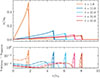 |
Fig. 4. Top: Flow profile of the self-similar Sedov-Taylor solution. The shock slows down over time ∝t−3/5. Here, Einj = 20, ρ0 = 1. Athena++ simulation (solid line) is compared to analytical profile with different shock widths, lsh = [0.1, 0.05, 0.01] (dashed, dash-dotted, dotted line). Bottom: Absolute error between the Athena++ simulation and approximated analytical profile. |
When simulating particle acceleration at such a blast wave, the inequality of (5) has to be fulfilled in the frame in which the shock is stationary ( ). For efficient acceleration, particles have to be confined; the characteristic acceleration time, κ/u2, should be short compared to the shock evolution time, R/u.
We first considered the case of a constant diffusion coefficient, κ. The maximal energy that can be reached at a given time can be calculated from Lagage & Cesarsky 1983; Drury 1983:
 (7)
(7)
where  ,
,  and, here, κ1 = κ2 = κ. With the rather unphysical condition of a constant diffusion coefficient, the maximal energy grows fast and particle feedback to the plasma cannot be neglected. The simulation is instead validated by comparing the estimated spectral slope. In the following section, the maximal energy is obtained considering Bohm diffusion.
When the shock radius, R, is large compared to the diffusion length scale, κ/u, the shock can be seen as a planar shock and we expect the energy spectrum at the shock to have the characteristic slope of s = −2. However, with increasing diffusion coefficient, the curvature of the shock has to be taken into account. In the limit where  is still a small parameter Drury 1983 gives an approximation of the spectral slope a at the shock,
![Mathematical equation: $$ \begin{aligned} a = 4 \left[1 + (3 + b) \left(\frac{\kappa _1}{R u_1} + \frac{\kappa _2}{R u_2}\right) + \frac{\kappa _2}{R u_2}\right] + O(\epsilon ^2), \end{aligned} $$](/articles/aa/full_html/2025/11/aa53593-24/aa53593-24-eq20.gif) (8)
(8)
where b describes the injection of particles, assuming f ∝ p−aR(t)b. Note that for ϵ → 0, the approximation yields the slope at a planar shock, f ∝ p−4. The small deviations from the planar solution originate from the finite rate at which particles are injected and accelerated (depending on the acceleration timescale, τacc = 3(κ1/u1 + κ2/u2)/(u1 − u2)), as well as the adiabatic cooling in the expanding flow behind the shock (determined by the downstream diffusive length scale κ2/u2).
At t = 0 the shock speed diverges and with that the advection profile given by Eq. (6) at r = 0. However, the blast wave approximation is only meant to be applied at late times, once the ejecta have swept out their own mass and the explosion can be treated as coming from a point source. At early times, the shock speed is high and acceleration is fast, as long as particles are confined by the shock. When simulating with CRPropa 3.2, acceleration is efficient when the inequality (5) involving the time step, shock width and diffusive step are fulfilled. Therefore the time step is chosen such that this is only true for t > 1, when the shock speed decreases to a reasonable speed.
Figure 5 shows the resulting distribution fp2 at t = 55 and t = 100, with the simulation parameters: Einj = 100, ρ0 = 1, κ = 0.01 and κ = 0.001, lsh = 0.01. A number of 106 pseudo-particles with p = p0 are injected homogeneously in the undisturbed medium at t = 0. Particles gain energy at the shock and can lose energy in the expanding flow behind the shock. Acceleration is fast at early times, when the shock speed is high; it slows down over time, so that the maximal energies reached at t = 55 and t = 100 are similar. This is in agreement with Eq. (7).
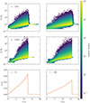 |
Fig. 5. Acceleration at the Sedov-Taylor blast wave. Particles are accelerated at the shock and then cooled in the expanding wind. |
Figure 6 shows the energy spectra at the shock at t = 100. With a sufficiently small diffusion coefficient, Eq. (8) yields a ≈ 4, the spectrum at a planar shock. With a higher diffusion coefficient, the resulting spectrum is steeper, which is in agreement with Eq. (8). For energy-dependent diffusion, this effect leads to a steepening of the spectral slope with increasing energy. The spectrum is affected by the finite size and acceleration time of the shock, a Hillas effect, and the adiabatic cooling in the downstream region of the shock due to the expanding flow. In the case of a spherical termination shock, there is a similar effect: particles are cooled upstream (which is inside) which leads to an enhancement in the energy spectrum at high energies right before the cutoff Drury 1983; Florinski & Jokipii 2003.
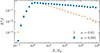 |
Fig. 6. Spectra at the shock at T = 100 for κ = 0.01, 0.001. The spectral slope matches the approximation given by Drury: s(κ = 0.001)≈2.075, s(κ = 0.01)≈2.75. |
3. Individual spherical shocks: Acceleration and escape back to the Galaxy
Strong SN explosions or SBs could lead to shocks propagating out of the Galaxy Tomisaka & Ikeuchi 1986; Dorfi & Breitschwerdt 2012 and it has been proposed that CRs could be accelerated at those local structures Dorfi et al. 2019. Like a potential Galactic wind termination shock, such outbursts would contribute to the CR spectrum in the transition region between the spectral knee and ankle Jokipii & Morfill 1987; Bustard et al. 2017; Merten et al. 2018; Mukhopadhyay et al. 2023. Although a Galactic termination shock is larger and could confine CRs at higher energies, the time-dependent structures are closer to the Galactic disk, making escape back to the Galaxy more promising. While Dorfi & Breitschwerdt 2012 and Dorfi et al. 2019 give an estimate on the maximal energy that could be reached at their shock structures, they do not discuss the probability of CRs returning back and how the transport affects the shape of the spectrum. For the termination shock, the escape back to the Galaxy would be upstream; in this scenario, downstream. However, the downstream frame is now moving with the (time-dependent) shock speed out of the Galaxy. All this combined suggests a non-negligible influence on the accelerated spectrum, s = −2.
We only expect shocks strong enough for particle acceleration when they run out of the Galactic disk and the density decreases. We refer to Weaver et al. 1977 for an estimate of the shock speed considering the constant density of the interstellar medium. Thus, starting from the Sedov-Taylor blast wave in Sect. 2.4, the flow profile is modified to take a decreasing density profile ρ ∝ 1/r2 into account. Furthermore, we consider a more realistic, energy-dependent diffusion coefficient compared to Sect. 2.4. When the mean-free path increases with energy, re-accelerated high-energy CRs have a higher probability of propagating back to the Galaxy. On the other hand, DSA is most effective for small diffusion coefficients. Thus, the Bohm limit is used in the following to evaluate the most promising scenario for a contribution to the flux in the knee to ankle regions.
3.1. Similarity solution with decreasing density
Outside the Galactic disk the density decreases and the shock can survive longer and propagate further out with higher velocities compared to the constant density scenario. While the original Sedov-Taylor solution assumes a constant density in the undisturbed medium, other similarity solutions consider different ambient media by introducing a power-law dependence of the density, ρ0(r) = Ar−ωIsenberg 1977. The velocity profile is then expressed as
 (9)
(9)
For ω = 2, the solution becomes critical with the simple linear profile V0 = 2/(γ + 1)λ, where γ = 5/3 and λ is the dimensionless parameter,
 (10)
(10)
of the similarity solution. The shock speed is then given by  . We restrict our analysis to the case ω = 2, for other values (ω < 3) the profile V0 is given in Isenberg 1977, for instance.
Figure 7 shows the resulting profile with A = ρ0r02 with r0 = 1 kpc and ρ0 = 1 mp/m3, where mp is the proton rest mass, in comparison to the one with constant density ρ0. The density is significantly higher for r < r0, thus, the value of ρ0 roughly leads to a reasonable density (specifically, this value of ρ0 gives ρ0(r = 1 pc) = 1 mp/cm3). For comparison, we also plot the Sedov-Taylor solution for constant density in Fig. 7. In addition to making it to larger radii, the shocks have larger speeds.
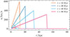 |
Fig. 7. Analytical solution of the Sedov-Taylor blast wave with constant density (dashed line) compared to the Isenberg solution with decreasing density profile (solid line) for Einj = 10 ESN, r0 = 1 kpc, and ρ0 = 1 mp/m3. Considerably higher shock speeds are reached for the latter. |
While such a flow profile is realistic for large radii, the density is overestimated for small r and diverges for r → 0. Thus, we expect it only to be valid at the larger scales, which are the relevant ones for the study here. As in Sect. 2.4 the constraints on the time step and shock width are chosen such that it is fulfilled for t > 1 Myr.
For the solutions shown in Figure 7, we use an injected energy of Einj = 10 ESN = 1052 erg. This energy is equivalent to ∼10 SN explosions all going off near each other in a short time frame. This assumption is reasonable for the initial burst of SNe in the early evolution of a star cluster (≳105 M⊙) (see Kim & Ostriker 2017 and references therein). Separating the individual SNe in time would require a numerical integration and a departure from the analytical solution that we pursued in this work.
Even so, the single summed injection is a good estimate at later times. Each individual shock would propagate through a lower density medium carved out by the previous shocks, eventually catching up and adding to the main shock, as long as they happen close together in time. For a similar result, consider the large bubble and outflow created by many individual shocks adding together in Dorfi et al. 2019. There could be some particle acceleration missed by not studying each SN shock individually as it catches up to the rest of the blast wave. However, it should be minimal because there will be a high sound speed interior to the total blast wave, so the follow-on shocks will tend to be rather weak.
3.2. Diffusion: Bohm diffusion at a parallel shock
DSA is most efficient for small diffusion coefficients. We consider strong turbulence close to the shock and Bohm diffusion coefficient following κ(p, r) = pc2/(3qB(r)). For efficient acceleration we assume the spherical shock to be parallel, thus, the magnetic field is radial at the shock. The magnetic field strength, B, decreases with 1/r2, hence, the Bohm diffusion coefficient increases. We set the magnetic field strength to B0 = 10 μG at r0 = 1 kpc.
The spatial dependence of the Bohm diffusion coefficient leads to a drift-like term in the SDE:
 (11)
(11)
which is implemented in the DiffusionTensor module and must be taken into account when constraining the time step (Eq. (5)). Depending on the energy and magnetic field strength, the drift-like term can get larger than the advection. It is, however, questionable if the diffusive regime is then still applicable.
We expect particles to be diffusive on the scales of the shock, when the diffusive length scale is smaller than the shock radius,  . With Einj = 10 ESN and the previously described density profile and magnetic field strength, the maximal rigidity, ℛ = E/q, that is still confined can be calculated and is shown in Fig. 8 depending on the shock radius, R. Similar considerations have been undertaken by, for instance, Lagage & Cesarsky 1983 and Drury 1983.
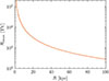 |
Fig. 8. To experience DSA, the diffusive length scale κ/u must be small compared to the shock radius R. With |


3.3. Estimate of the maximal energy
With the shock speed and diffusion coefficient, the maximal energy that can be reached at a time t is estimated by integrating Eq. (7)
 (12)
(12)
where the magnetic field is evaluated at the shock radius and R and  depend on time. With C = qcB0r02/15 and E ≈ pc follows
![Mathematical equation: $$ \begin{aligned} E_{\rm max}(t) = C \left[\frac{1}{t_0} - \frac{1}{t}\right] + E_0, \end{aligned} $$](/articles/aa/full_html/2025/11/aa53593-24/aa53593-24-eq30.gif) (13)
(13)
which is independent of the injected energy, Einj, and with that the shock speed. This is due to the decreasing magnetic field: With higher shock speed, radii with low magnetic field are reached faster, and the acceleration is slowed down. Thus, for the considered flow profile the effect of a higher shock speed on the acceleration time is canceled out by the higher diffusion.
The resulting maximal energy for B0 = 10 μG, r0 = 1 kpc, t0 = 1 Myr and E0 = 100 TeV is shown in Fig. 9 and goes up to 2 PeV.
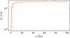 |
Fig. 9. Estimate of the maximal energy that protons reach at the shock over time for B0 = 10 μG, r0 = 1 kpc, t0 = 1 Myr and E0 = 100 TeV. |
3.4. Simulation setup
Candidates are injected at t = 0 with an energy spectrum E−1 from TeV to 100 TeV in the volume r < 60 kpc. From Fig. 8 it is clear that for r > 60 kpc re-accelerated particles with higher energy than PeV are not diffusive on the scales of the shock and are not well described in the ensemble-averaged regime. The injected energy spectrum is re-weighted in the later analysis to E−2. With Einj = 10 ESN, r0 = 1 kpc and ρ0 = 1 mp/m3 the expanding shock reaches a radius of 60 kpc at t ≈ 80 Myr. All Candidates are protons, since interactions are not considered the result can be applied to heavier particles with the same rigidity as well. The CandidateSplitting module is used to increase statistics at high energy.
To investigate the effect of the shock speed and the magnetic field strength on the maximal energy and transport back to the Galaxy, three simulations are performed: [Einj = 10 ESN, B0 = 10 μG], [Einj = 100 ESN, B0 = 10 μG], [Einj = 10 ESN, B0 = 100 μG].
3.5. Adaptive step: Energy-dependent shock width
The small Bohm diffusion coefficient, κ(TeV, r0) = 1.5 × 1023 cm2 s−1, requires a small shock width lsh, so that the mean diffusive step is larger than the shock width. On the other hand, a small shock width affords a small time step, since the advective step has to be smaller than the shock width. At t = 1 Myr and r = R(1 Myr), a time step of Δt = 10−5 Myr fulfills the constraints considering pseudo-particle energies of TeV. We expect re-acceleration up to 10 PeV, thus, the diffusive step increases by a factor larger than 1000. However, the diffusive step has to be on the order of the shock width, otherwise pseudo-particles do not encounter the shock (Kruells & Achterberg 1994, A24).
The previously implemented adaptive step (A24, MA25) scales the time step down to keep the diffusive step within bounds. Here, the time step is already quite small, decreasing it further would lead to high computation times. Instead, we scale the shock width with the square root of the pseudo-particles’ energy. At this point, we emphasize again that the shock width does not have to be equal to the physical width of the shock.
3.6. Simulation results
Figure 10 shows the resulting number density fp2 at two times. Particles are accelerated up to 50 PeV. High-energy particles experience high diffusion and drift ∂κ/∂r and quickly move out of the Galaxy. Particles above the orange line do no longer fulfill the criterion  , meaning they are not properly described by the diffusion ansatz. Since in the further analysis (see Fig. 11) we focus on the particle spectra at the shock, we do not expect a large difference on short timescales between the diffusive particle population and the ballistic one. The other observer position is at r = 5 kpc, where almost all particles are diffusive for all times.
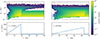 |
Fig. 10. Flow profiles and space-energy histogram at t = 18 Myr and t = 62 Myr for E0 = 10 ESN, B0 = 10 μG. Particles are accelerated close to the Galaxy, when the shock speed is high and diffusion low. The orange line indicates the maximal energy protons are still diffusive. |
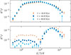 |
Fig. 11. Energy spectra over time at the moving shock (top) and at 5 kpc (bottom) for E0 = 10 ESN, B0 = 10 μG. Only particles with sufficiently high energy make it back to the Galaxy. |
Figure 11 shows the spectra at the moving shock at different times. It can be divided into three parts: The injected energy range Einj = [TeV, 100 TeV], the cooled energy range Ecool < TeV, and the re-accelerated range Eacc > 100 TeV. The injected energy range flattens over time, which is an artifact of the finite injection range: low-energy particles are accelerated up to higher energies and increase the flux. Without the minimum injected energy, the loss of accelerated particles at such energies would be compensated by the acceleration of particles from even lower energies. Cooling also flattens the spectrum: high-energy particles spend less time, on average, in the expanding flow. This is well visible in the cooled energy range.
The re-accelerated energy range has a spectral slope ≤2. For energy-dependent diffusion, it follows from Eq. (8) that the spectrum steepens with increasing energy. Note that this occurs even below the cutoff energy due to finite acceleration time and size of the accelerator. For energy > 100 TeV, the steepening of the spectrum is well visible in Fig. 11.
Interestingly, the energy spectrum at the shock also slightly steepens over time. The shock slows down and, thus, accelerates particles to a steeper spectrum. Particles are cooled in the downstream region of the shock. When the shock is not fast enough to compensate for the energy losses anymore, the spectrum steepens. Also, the shock propagates in an area with lower magnetic field and without further magnetic field amplification, the diffusion coefficient increases. Taking both effects into account, Eq. (8) predicts a steepening of the spectrum with time.
The bottom panel of Fig. 11 shows the energy spectrum at r = 5 kpc for an estimate of the particle spectrum that escapes back to the Galaxy. It can be divided into the injected part that is cooled and advected outwards over time, and the re-accelerated part that is able to diffuse back. While the low-energy part decays over time, the re-accelerated part is less affected by advection and is almost stationary.
We further investigate the impact of the shock speed by increasing the energy of the explosion to E0 = 100 ESN (left column of Figs. 12 and 13) and the impact of the diffusion coefficient by amplifying the magnetic field to B0 = 100 μG (right column of Figs. 12 and 13). The magnetic field can be amplified due to the Bell instability driven by the CRs themselves Bell 2004; Amato & Blasi 2009. A high magnetic field is key to confine and accelerate CRs at shocks, and it has been proposed that the Bell instability leads to significant amplification Zweibel & Everett 2010; Drury & Downes 2012.
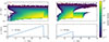 |
Fig. 12. Flow profiles and space-energy histogram at t = 20 Myr for E0 = 100 ESN, B0 = 10 μG (left) and for E0 = 10 ESN, and B0 = 100 μG. The orange line indicates the maximal energy protons are still diffusive for the respective magnetic field and shock speed. |
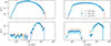 |
Fig. 13. Energy spectra over time at the moving shocks (top) and downstream (bottom) at 5 kpc at for E0 = 100 ESN, B0 = 10 μG (left) and E0 = 10 ESN, and B0 = 100 μG (right). |
With a higher injected energy the shock speed increases. Like predicted in Eq. (12) the maximal energy reached at the shock is the same ≈10 PeV. Fewer low-energy particles make it back to the Galactic boundary since they are advected out with the faster flow. In this scenario, the maximal energy is independent of the individual energy in the outbursts. If, however, the magnetic field strength or the density decrease with a different dependency on r, the maximal energy would change.
With a smaller diffusion coefficient, particles are accelerated to a harder spectrum and reach higher maximal energy. However, because of the decreased diffusion coefficient, the particles are advected outwards more efficiently. Therefore, fewer particles make it back to the Galaxy.
4. Consecutive planar shocks: Softer spectra and collisions
With explosions like the one discussed in the previous section happening frequently in the Galaxy, a stationary flux could develop. Also, shocks are likely to run into each other and their interaction would result in complex landscapes affecting CR acceleration and their transport back to the Galaxy.
We approach the idea of CR acceleration at interacting shocks by considering two 1D planar shocks, one emerging after the other. From the Rankine-Hugoniot conditions follows, that the second shock is faster than the first shock: The shock has to be faster than the speed of sound, cs, in the preshock medium; otherwise, it does not fulfill the Mach criterion: M > 1, with M2 = u2/cs2. When the preshock medium is already shocked and in motion, it follows
 (14)
(14)
where
 (15)
(15)
assuming a non-relativistic fluid with γ = 5/3. For the speed of the second follows from Eq. (14):  . The compression of the shock changes, likely ending up being lower than 4.
For secondary SN or SB explosions, this means that their energy must be significantly higher to produce a flow which is a second shock. When radiative cooling or spherical expansion (e.g., a Sedov-Taylor blast wave) is taken into account, this constraint becomes less severe, since the velocity behind the first shock can be lower. Dorfi et al. 2019 confirmed with their hydrodynamic simulation, considering a flux tube geometry, that secondary shocks are always faster than the previous shocks and eventually collide.
4.1. Colliding shocks
We considered two 1D planar shocks propagating in the same direction and ask what happens when they collide. A new Riemann problem emerges, with the undisturbed medium (0) on one side and the twice shocked medium (2) on the other. From Courant & Friedrichs 1999, we know that a contact discontinuity forms and a rarefaction wave travels backward, as sketched in Fig. 14.
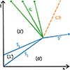 |
Fig. 14. Sketch of the colliding shock problem: Two shocks start at x = 0 at different times, the second shock is faster than the first and catches up. When they collide a new Riemann problem forms determined by the states (0) and (2). Three new regions develop: The shocked medium between the single shock S′ and the contact discontinuity (CD), the medium between the CD and the rarefaction wave (R), and the rarefaction wave itself. Pressure and velocity do not change over the CD. The rarefaction wave travels at the local sound speed. The sound speed differs at the head and tail of the rarefaction wave, as indicated by the three rays. |
For more quantitative statements, for instance, on the speed of the new shock, the scenario can be viewed as a modification of the Sod shock tube problem Sod 1978. This is a widely used test case for hydrodynamic codes, where the initial condition for density and pressure on one side of a 1D domain are chosen high but low on the other side. The pressure and density gradient drive a shock wave when the simulation starts. The original problem from Sod 1978 has set values for each quantity and region. For example, the speed on both sides is set to zero. In the Riemann problem we aim to solve, the high pressure/high density medium is already in motion. Therefore, we build a two-shock initial condition from the generalized shock tube problem already in Athena++.
The (single) shock tube problem can be solved analytically with the Rankine-Hugoniot conditions; however, the pressure and velocity on both sides of the contact discontinuity have to be calculated iteratively. Instead, we set up the modified shock tube problem in Athena++ to obtain pressure, density and velocity in the unknown region. Note that the density changes over the contact discontinuity, but not the pressure or velocity. Those simulated values are used to construct the analytical profile for the full velocity profile and its derivative, which is necessary for modeling the particle acceleration with CRPropa (see Fig. 15).
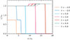 |
Fig. 15. Athena++ simulation of colliding shocks with vsh, 1 = 1, vsh, 2 = 2 (solid line) and corresponding Sod shock tube (dashed line) with vR = 1.5, vL = 0. The shocks collide at x = 8 at t = 0, which is when the Sod shock simulation starts. |
We considered two shocks with high speed that could be produced in the Galactic disk and move outwards. We set the first shock’s velocity as vsh, 1 = 400 km/s and the second shock’s velocity to be twice as large vsh, 2 = 2vsh, 1 = 800 km/s (note this value satisfies Eq. (14)). The shock speeds are in agreement with several papers on Galactic outflows or winds, for instance, Bustard et al. 2016; Mukhopadhyay et al. 2023; Dorfi & Breitschwerdt 2012. The effect on the energy spectrum is similar also for other shock speeds, as long as the effective compression ratio is considerably changed. Since the first shock moves into a low pressure medium it has a compression of 4 and, thus, accelerates particles to a spectrum with −2 slope. The compression ratio of the second shock is only q = 2.5, so it produces a steeper spectrum s = 2 − 3q/(q − 1) = − 3 Drury 1983.
By considering planar shocks, we solely investigate the impact of the colliding shocks on the energy spectrum, without any influence from the shock geometry or spherical expansion.
4.2. Diffusion: Bohm diffusion in constant magnetic field
As in the previous section we consider Bohm diffusion, κ = 1/3(pc/(qB)). Here, the magnetic field strength stays constant and B = 1 μG. Thus, the diffusion coefficient only scales with momentum and the drift term vanishes, ∂κ/∂z = 0.
In contrast to spherical shocks, for 1D planar shocks, there are no geometric constraints for the confinement of particles. However, it is questionable if particles with energy higher than 10 − 100 PeV find waves to scatter with. If not, the ensemble-averaged description is not applicable.
4.3. Estimate of the maximal energy
An estimate of the maximal energy reached at one individual shock over time is obtained from Eq. (7) analogous to the previous section. Here, the shock speed does not change over time. Assuming Bohm diffusion, the maximal energy is
 (16)
(16)
The maximal energy grows linearly in time and is shown for protons in Fig. 16 for B = 1 μG, vsh = 400 km/s and E0 = TeV.
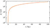 |
Fig. 16. Estimate of the maximal energy that protons reach at a single shock over time for B0 = 10 μG, vsh = 400 km/s and E0 = 1 TeV at t0 = 0. |
4.4. Estimate of the spectral slope
It has been suggested that such a system of shocks produces broken power laws since the compression ratio of the subsequent shocks is lower. However, when two shocks are catching up with each other, at some point particles may be able to encounter both shocks, when their diffusion coefficient is large enough (see also the work by, e.g., Bykov et al. 2013; Wang et al. 2019; Vieu et al. 2020 for similar considerations in steady-state and time-dependent colliding/converging shock waves)2. In that case, the spectrum at the shock(s) should harden, since the total compression ratio is higher. Another way to interpret this is that the escape probability is changed. Here, the total compression ratio would be q = q1q2. For our simulations with vsh, 2 = 2vsh, 1, we have q = 10 and a corresponding spectral slope s ≈ −1.33. However, there is only a finite time, namely the time until the shocks collide, to actually accelerate particles to that harder spectrum.
For the spectrum to be accelerated up to the slope that corresponds to the total compression ratio, the diffusion timescale, τdiff = Δx2/κ(p), where Δx is the distance of the shocks, must be equal to the acceleration timescale, τacc. Microscopically, each particle is then as likely accelerated at the first shock as it will encounter the second shock. When the diffusive timescale is longer but still on the order of the acceleration time, the hard spectrum cannot fully develop and the resulting spectral slope is somewhere between s(q1) and s(q1q2). Considering Bohm diffusion, Fig. 17 shows the acceleration timescale of the first shock τacc, I and second shock τacc, II and the diffusion timescale for different distances Δx between the two shocks depending on the particle’s momentum. Particles having a momentum on the order of the momentum defined by the crossing of the timescales or higher (p > pcross, with τacc(pcross) = τdiff(pcross)) are able to probe both shocks and are accelerated to a flatter (harder) spectrum than the one expected by an individual shock. The collision time is indicated by the dotted lines in Fig. 17. Note that they might have an acceleration timescale that is higher than the time left until the shocks collide.
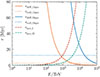 |
Fig. 17. Time scales depending on the particles energy: Acceleration times at the respective shocks (dashed lines) increase with energy. The diffusive timescale (solid) for two different distances between the shocks Δx = [1, 5] kpc decreases with energy. The collision time depending on Δx is indicated by the dotted lines. |
In this scenario, we expect a flattening of the spectrum only for high-energy particles (> PeV) shortly before the shocks collide: (1) Particles need to be accelerated first to sufficiently high energy. The closer the shocks are, the lower is the critical energy to probe both shocks. (2) The timescale to accelerate to the harder spectrum must be on the order of the collision time. This constraint is easier to fulfill at the faster, second shock.
4.5. Simulation setup
Candidates are injected at t = 0 monoenergetically with E = 1 TeV uniformly in the range z = [0, 60] kpc. The first shock is launched at t = 0 with the speed vsh, 1 = 400 km/s, the second shock emerges after ΔT with the speed vsh, 2 = 800 km/s. The simulation ends at t = 100 Myr and two time offsets between the shocks ΔT = [25, 40] are tested.
The diffusive step  , increases with energy. Here, the shock width is not scaled with energy since we are interested in the interaction of the two shocks. Scaling the shock width with energy would cause different merging times as a function of pseudo-particle energy. Instead, the time step Δt is scaled linearly with the energy to keep the diffusive step within bounds and to fulfill Eq. (5).
Again, the CandidateSplitting module is used to increase statistics at high energy.
4.6. Simulation results
Figure 18 shows the space-energy histogram at two times, before and after the collision of the shocks. In Fig. 19, we show the spectra at the first shock, the second shock launched 40 Myr after the first, and the one that emerges after the collision at t = 80 Myr.
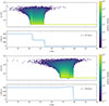 |
Fig. 18. Flow profiles and space-energy histogram at t = 67 Myr before the collision and t = 89 Myr. Particles are accelerated fast and the characteristic upstream and downstream spectra are visible for energy-dependent diffusion. |
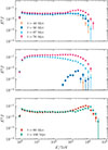 |
Fig. 19. Energy spectra over time at the first shock (top), the second shock (middle) and the shock after collision (bottom). With ΔT = 40 Myr the shocks collide at t = 80 Myr. Around the collision, the spectrum flattens for E > PeV right before the energy cutoff. |
Particles reach high energy quickly, which is in agreement with Eq. (16). The first shock drags the particles along and at early times, only the high-energy particles can be re-accelerated at the second shock (see, e.g., t = 56 Myr in Fig. 19). At later times, the full downstream spectrum of the first shock reaches the second (t = 67 Myr one as can be seen in Fig. 19). The second shock also pushes the particles back to the first one, which impacts in particular the low-energy particles (see the upper panel of Fig. 18). The flux E2J is therefore higher at the second shock. At t = 78 Myr, shortly before the shocks collide, the spectrum at the second shock flattens. At the first shock, a flattening at high energies E > PeV right before the energy cutoff becomes visible. This is consistent with the findings by Vieu et al. 2020.
Once the shocks collide, the new shock emerges. It is faster than both of the previous ones and accelerates particles to even higher energy (see Eq. (16)). Behind the shock a rarefaction wave develops and particles are cooled in that region. The flattening of the spectrum at high energies is still visible; however, the shock goes on to accelerates particles to a −2 spectrum as it is, again, a strong shock. From the merger on, again only low-energy particles, E0 = 1 TeV, are injected at the shock; thus, we expect the spectrum to relax back to a −2 slope.
Figure 20 shows the spectra at the single shock after a collision at 50 Myr. The second shock emerged faster, 25 Myr after the first. At t = 100 Myr, the spectrum is a single power law with −2 slope again. Thus, in this scenario, the flattening of the spectrum is a transient effect.
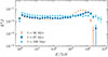 |
Fig. 20. Energy spectra over time at the shock after collision. With ΔT = 25 Myr the shocks collide at t = 50 Myr. Over time, the new shocks accelerates particles to higher energy with −2 slope and the bump at high energy disappears. |
4.7. Propagation back to the Galaxy
Without cooling, only few particles of the highest energy make it back to the Galactic disk in Fig. 18. Such shock profiles are only expected locally, in a magnetic flux tube and for a finite time. For an estimate, we assume that the wind ceases after 100 Myr. The re-accelerated particles can now diffuse back to the Galaxy without going against the flow, and the time evolution of the number density n becomes
 (17)
(17)
where the diffusion coefficient remains spatially constant. The spectra that come back to z = 5 kpc are obtained from the convolution of the particle distribution at t = 100 Myr with the Green’s function of the pure diffusion equation
 (18)
(18)
where z0 is the particles’ position at t = 100 Myr and p0 their momentum. Without the background flow, there are no processes to gain or lose energy. We test two diffusion scenarios: Bohm diffusion κ = pc/(qB) and Galactic diffusion κ = 5 × 1024 m2/s (E/GeV)1/3.
Figure 21 shows the particle spectra at z = 5 kpc for different time durations after the wind has ceased. For Bohm diffusion, only particles re-accelerated to high energy make it back to the Galaxy, similar to the results obtained in the previous section for a spherical shock. At late times, more low-energy particles (< PeV) contribute and the peak of the spectrum shifts to lower energy. The high-energy particles (> PeV) spread over a wider distance and the probability to find them at 5 kpc decreases. The difference in the spectra between ΔT = 25 Myr and ΔT = 40 Myr between the two shocks is negligible.
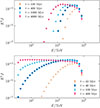 |
Fig. 21. Spectra at x = 5 kpc at different times t after the wind stopped at t = 100 Myr. The spectra are obtained from the convolution with the Green’s function of the pure diffusion equation. Top: Bohm diffusion. Bottom: Galactic diffusion. |
The Galactic diffusion coefficient is higher, and the timescale at which high-energy particles make it back is shorter. Also, 100 Myr after the wind has stopped, a significant amount of particles with energy < 100 TeV arrives at 5 kpc.
5. Discussion
We have investigated a number of scenarios that contribute to the dynamical shock landscape forming in the Galactic halo: strong explosions, resulting from several SN or SB outbursts, run out of the Galactic disk and experience a decreasing density profile. We find that such shocks are strong enough to accelerate particles up to the spectral knee. With SN or SB explosions happening frequently in the Galaxy, they are bound to interact with each other Dorfi et al. 2019. Thus, we studied the scenario of two shocks that catch up with each other and eventually collide. In both scenarios, we obtained the time-dependent spectra at the respective shocks and the spectrum of particles that is able to diffuse back to the Galaxy and contribute to the CR spectrum. We used a modified version of CRPropa that facilitates time-dependent advection profiles to simulate test particle transport and acceleration.
We note that with the test particle approach of CRPropa, we currently cannot model any influence of CRs on the plasma. This means non-linear feedback of the CRs on the plasma flow as, for instance, in Blasi 2002 or on the gas compression ratio as, for instance, in Ellison & Eichler 1985. Any such non-linear correction would lead to modification of the expected spectral index of the accelerated CRs. In the future, some of these effects might be taken into account but this is beyond the scope of this paper.
In Sect. 2, we describe how we used predictions for the maximal energy and spectral slope at a Sedov-Taylor blast wave to validate the new code. For spherical, expanding shocks the spectral slope can deviate from the well-known −2 slope obtained for planar shocks, due to the different injection rate at the shock (the shock surface grows with time) and adiabatic cooling in the expanding flow on the downstream side of the shock. The correction is negligible if the diffusion coefficient is small compared to the shock radius and shock speed,  .
.
With energy-dependent diffusion, this effect may become important for high-energy particles, leading to a steepening of the spectrum before the cutoff. In our scenario, where we consider Bohm diffusion in a decreasing magnetic field, B ∝ r−2, and CR are assumed to be pre-accelerated to energies up to 100 TeV, we find that they are re-accelerated to a steeper spectrum s < −2 for energies in the range 10 − 100 PeV. Thus, the steepening of the spectrum between the knee and ankle could partially be a result of the shock’s geometry and magnetic field turbulence.
To accelerate particles up to that energy, the shock speed needs to be high enough, which we only find for Eblast = 10 − 100 ESN when the density decreases with distance to the Galaxy. Here, we used ρ ∝ r−2 to employ the critical solution found by Isenberg 1977. This is reasonable when the outburst happens close to the edge of the Galactic disk or when another explosion previously happened in the vicinity and swept the surrounding mass away.
We find that re-accelerated particles from 100 TeV to 100 PeV make it back to the Galaxy. Although the 100 PeV limit is only reached when the magnetic field is strong/diffusion is small. Since the flow expands and slows down over time, it is easier for CR to propagate back than, e.g., in the scenario of a Galactic wind termination shock, where particles need to escape upstream and diffuse against the strong, unshocked wind (e.g., Jokipii & Morfill 1987; Merten et al. 2018). Also, the distance they must cover is way smaller than in the case of a Galactic termination shock at r ≈ 200 kpc. We even find that the flux from 100 TeV to 100 PeV is rather stationary and does not change much on timescales of 80 Myr after the explosion. This is due to the small diffusion and advection speed close to the Galaxy. Thus, only a few strong explosions in the past are required to obtain a stationary flux in that energy range.
The considered spherical geometry has, on the other hand, a disadvantage for the low energies: CR with small diffusion coefficients (E < 100 TeV) are pulled outwards with the flow and their flux decreases over time. However, in reality, such outbursts are likely not spherically symmetric. The global structure is likely asymmetric, and the explosion will depend significantly on the local environment of the SB. A more realistic shock could probably re-accelerate CR to high energies (≳PeV) without reducing the number of low-energy CRs. In particular, the Kompaneets solution Kompaneets 1960 for an explosion in an exponentially stratified surrounding medium leads to an ellipsoidal shaped shock that can efficiently accelerate CRs Dorfi et al. 2019. In order to apply our model, the resulting time- and space-dependent velocity profile must be known.
Furthermore, a reverse shock is expected to run backwards, towards the Galaxy but advected out with the flow Dorfi & Breitschwerdt 2012. The shock forms when the swept-up mass is significantly larger than the injected mass. The reverse shock is not captured by the similarity solution we applied. However, it might have an impact on the particle acceleration; re-accelerating particles that escape downstream as found in SNRs Brose et al. 2019.
It is interesting to further investigate the transport of CR that were re-accelerated at such local outbursts, allowing for a more detailed study on the transport regimes and the magnetic field geometry, which is beyond the scope of this work. The spectrum at the shock can be split up in two parts that are treated in a diffusive and ballistic way, respectively. The transition from diffusive to ballistic transport is already indicated, for instance, in Fig. 10. Furthermore, the diffusion coefficient could increase to the Galactic value for CRs that escape the region close to the shock with amplified magnetic field. As shown in Fig. 21 it is more likely that they diffuse back.
Interestingly, the re-accelerated CR flux that comes back to the Galaxy is stationary on timescales ≲80 Myr. Thus, in order to explain a stationary flux in that energy range, the strong outbursts do not necessarily have to happen frequently. A spiral magnetic field structure would further delay the CR arrival time Merten et al. 2018 and with that, past explosions, when the Galaxy was more active in star formation (see, e.g., Freundlich 2024 for the general time evolution of the star formation rate), could still contribute to the spectrum above the spectral knee.
The amount and frequency of such explosions can be constrained by a transport study of CRs from various outbursts back to Earth. The source regions can be placed randomly in the Galaxy and in time (see Mertsch 2018 for a similar study). The source distribution can match the current structure of star forming regions Zhang et al. 2024. These studies could constrain the anisotropy of arrival directions in the respective energy range.
We investigated the case of two consecutive shocks. Considering planar shocks, the second one has to be faster than the first. This is also true in a flux tube geometry, when the density behind the first shock decreases and was found from simulation by Dorfi et al. 2019. We further showed that the profile can be described by a modified version of the Sod’s shock tube problem, which has an analytic solution. Using results from Athena++ simulations of the colliding shocks, we constructed the advection profile and its derivative for use in CRPropa, allowing us to model particle transport and acceleration. The 1D model considered here sets the most stringent criterion possible for shocks to collide. Dropping the assumption would allow shocks with different launch footprints to collide obliquely which also produces a region of shear, which might become turbulent and in which the magnetic field might be amplified.
For the resulting energy spectrum, there are two predictions: with the secondary shocks having a lower compression ratio, the energy spectrum of particles re-accelerated at those shocks steepens. And when shocks are close to each other and particles encounter both shocks, the energy spectrum may become harder.
In our scenario, we do not find a steepening of the energy spectrum at the second shock. First, only high-energy particles reach the second shock and their acceleration timescale is too long to see the steepening of the spectrum (in contrast to the cutoff). Later, the acceleration process is constrained by the time left before the merger. However, when taking cooling (e.g., due to spherical expansion) into account, the downstream spectrum of the first shock could reach the second shock more easily against the wind. Thus, it could be re-accelerated by the second, less compressed shock, likely to a steeper spectrum.
We only find harder spectra close to the collision time similar to the analysis by Vieu et al. 2020 for converging flows. The diffusive timescale, Δx2/κ, and the acceleration time scale, ∝κ, must be on the same order, which is only fulfilled when the shocks are already close. The spectrum relaxes back after the collision, when the newly formed shock accelerates particles again to a −2 spectrum. Nevertheless, we find the effect interesting, in particular in systems where the shocks can be assumed stationary and the acceleration time is not constrained by the collision time (e.g., Bykov et al. 2013; Malkov & Lemoine 2023). Furthermore, the time-dependent test particle simulations with CRPropa can be extended to systems with more complex geometry and/or diffusion tensors.
In the case of 1D planar shocks, the flow speed remains high without radiative cooling and prevents particles from diffusing back to the Galaxy even if they escape downstream. Considering a spherical expansion, particles are more likely to propagate back, but are also subject to cooling. However, considering a finite lifetime of the shock (here we used 100 Myr as in Merten et al. 2018 for the Galactic wind termination shock), particles have a higher chance to diffuse back to the Galaxy. We convolved the energy spectra at 100 Myr with the Green’s function of the pure diffusion equation to find the time-dependent spectra at the Galactic boundary. As the analytic solution for the pure diffusion transport equation is known, no additional simulation has to be done for this. This has the advantage that different diffusion scenarios for the time after the wind ceased can be tested easily.
Depending on the diffusion coefficient, only the particles re-accelerated to high energies E > PeV or the full spectrum E > TeV make it back to the boundary within ≈400 Myr. Thus, a good description of the diffusion properties is crucial to obtain results that can be fitted to data. Considering a more realistic magnetic field structure, the arrival times at the Galactic boundary will change and likely become latitude dependent. Together with a study on the anisotropy of the diffusion coefficient, predictions for the anisotropy of the CR flux can also be made (see, e.g., Merten et al. 2018).
In summary, we have presented a modified version of CRPropa that facilitates time-dependent advection profiles. We validated the new code by simulating particle acceleration at a Sedov-Taylor blast wave. We further applied this code to two acceleration scenarios: at a shock driven by an explosion that runs out of the Galaxy and at two shocks catching up with each other and colliding. In both cases, we find that protons can be accelerated up to 10 − 100 PeV, depending on the shock speeds and magnetic field strength and turbulence. Since the shocks are closer to the Galaxy than a Galactic wind termination shock, particles are more likely to diffuse back to the Galactic boundary; either against the expanding wind or after the wind has ceased. Furthermore, we find that as the two shocks get close to one another, the spectrum hardens as particles encounter both shocks.
The results can be applied also to other galaxies in the future. Even though the downstream escape is towards the galaxy, re-accelerated particles could escape the galaxy once the wind ceases. This case is similar to the study described in Sect. 4.7. Furthermore, the transport and acceleration of electrons can be modeled to predict the inverse Compton and synchrotron emission on shocks in the Galactic halo, as predicted by Zhang et al. 2024.
See the GitHub repository for details and installation instruction https://github.com/CRPropa/CRPropa3
While writing up the manuscript we became aware of the work by Vieu et al. 2020. Their considerations for converging shock waves are similar to ours for colliding shocks, although not the same. Nevertheless, the resulting energy spectra agree very well.
Acknowledgments
SA, LM, and JBT acknowledge support from the Deutsche Forschungsgemeinschaft (DFG): this work was performed in the context of the DFG-funded Collaborative Research Center SFB1491 “Cosmic Interacting Matters – From Source to Signal” (grant no. 445990517). RH and EZ acknowledge support from NASA FINESST grant No. 80NSSC22K1749 and NSF grant AST-2007323 and PHY-2409224 during the course of this work. This work was supported by the Ruhr University Research School, funded by Germany’s Excellence Initiative [DFG GSC 98/3] (research stay by SA). This work has made use of the following software packages: Athena++ Stone et al. 2020, CRPropa Alves Batista et al. 2022, matplotlib Hunter 2007, numpy Harris et al. 2020, pandas McKinney 2010, and jupyter Kluyver et al. 2016. We acknowledge useful comments by the referee that improved the paper.
References
- Abaroa, L., Romero, G. E., Mancuso, G. C., & Rizzo, F. N. 2024, A&A, 691, A93 [NASA ADS] [CrossRef] [EDP Sciences] [Google Scholar]
- Achterberg, A., & Schure, K. M. 2011, MNRAS, 411, 2628 [CrossRef] [Google Scholar]
- Aerdker, S., Merten, L., Becker Tjus, J., et al. 2024, JCAP, 2024, 068 [CrossRef] [Google Scholar]
- Alves Batista, R., Becker Tjus, J., Dörner, J., et al. 2022, JCAP, 2022, 035 [CrossRef] [Google Scholar]
- Amato, E., & Blasi, P. 2009, MNRAS, 392, 1591 [Google Scholar]
- Becker Tjus, J., & Merten, L. 2020, Phys. Rep., 872, 1 [NASA ADS] [CrossRef] [Google Scholar]
- Bell, A. R. 2004, MNRAS, 353, 550 [Google Scholar]
- Bell, A. R., & Lucek, S. G. 2001, MNRAS, 321, 433 [CrossRef] [Google Scholar]
- Bell, A. R., Matthews, J. H., Taylor, A. M., & Giacinti, G. 2025, MNRAS, 539, 1236 [Google Scholar]
- Blasi, P. 2002, Astropart. Phys., 16, 429 [NASA ADS] [CrossRef] [Google Scholar]
- Brose, R., Sushch, I., Pohl, M., et al. 2019, A&A, 627, A166 [NASA ADS] [CrossRef] [EDP Sciences] [Google Scholar]
- Bustard, C., Zweibel, E. G., & D’Onghia, E. 2016, ApJ, 819, 29 [NASA ADS] [CrossRef] [Google Scholar]
- Bustard, C., Zweibel, E. G., & Cotter, C. 2017, ApJ, 835, 72 [NASA ADS] [CrossRef] [Google Scholar]
- Bykov, A. M., & Fleishman, G. D. 1992, MNRAS, 255, 269 [NASA ADS] [CrossRef] [Google Scholar]
- Bykov, A. M., Gladilin, P. E., & Osipov, S. M. 2013, MNRAS, 429, 2755 [Google Scholar]
- Castor, J., McCray, R., & Weaver, R. 1975, ApJ, 200, L107 [NASA ADS] [CrossRef] [Google Scholar]
- Courant, R., & Friedrichs, K. O. 1999, Supersonic Flow and Shock Waves (Springer Science& Business Media), 21 [Google Scholar]
- Dorfi, E. A., & Breitschwerdt, D. 2012, A&A, 540, A77 [NASA ADS] [CrossRef] [EDP Sciences] [Google Scholar]
- Dorfi, E. A., Steiner, D., Ragossnig, F., & Breitschwerdt, D. 2019, A&A, 630, A107 [NASA ADS] [CrossRef] [EDP Sciences] [Google Scholar]
- Drury, L. O. 1983, Rep. Prog. Phys., 46, 973 [Google Scholar]
- Drury, L. O., & Downes, T. P. 2012, MNRAS, 427, 2308 [NASA ADS] [CrossRef] [Google Scholar]
- Ellison, D. C., & Eichler, D. 1985, Phys. Rev. Lett., 55, 2735 [Google Scholar]
- Florinski, V., & Jokipii, J. R. 2003, ApJ, 591, 454 [Google Scholar]
- Freundlich, J. 2024, Fund. Plasma Phys., 11, 100059 [Google Scholar]
- Habegger, R., & Zweibel, E. G. 2024, ArXiv e-prints [arXiv:2412.12249] [Google Scholar]
- Habegger, R., Zweibel, E. G., & Wong, S. 2023, ApJ, 951, 99 [NASA ADS] [CrossRef] [Google Scholar]
- Harris, C. R., Millman, K. J., van der Walt, S. J., et al. 2020, Nature, 585, 357 [NASA ADS] [CrossRef] [Google Scholar]
- Hillas, A. M. 2005, J. Phys. G Nucl. Phys., 31, R95 [NASA ADS] [CrossRef] [Google Scholar]
- Hunter, J. D. 2007, Comput. Sci. Eng., 9, 90 [NASA ADS] [CrossRef] [Google Scholar]
- Isenberg, P. A. 1977, ApJ, 217, 597 [Google Scholar]
- Jokipii, J. R., & Morfill, G. 1987, ApJ, 312, 170 [Google Scholar]
- Kahn, F. D. 1975, Int. Cosmic Ray Conf., 11, 3566 [NASA ADS] [Google Scholar]
- Kim, C.-G., & Ostriker, E. C. 2017, ApJ, 846, 133 [NASA ADS] [CrossRef] [Google Scholar]
- Kluyver, T., Ragan-Kelley, B., Pérez, F., et al. 2016, Positioning and Power in Academic Publishing: Players, Agents and Agendas (Netherlands: IOS Press), 87 [Google Scholar]
- Kompaneets, A. S. 1960, Sov. Phys. Dokl., 5, 46 [NASA ADS] [Google Scholar]
- Kopp, A., Büsching, I., Strauss, R. D., & Potgieter, M. S. 2012, Comput. Phys. Commun., 183, 530 [NASA ADS] [CrossRef] [Google Scholar]
- Kruells, W. M., & Achterberg, A. 1994, A&A, 286, 314 [NASA ADS] [Google Scholar]
- Lagage, P. O., & Cesarsky, C. J. 1983, A&A, 125, 249 [NASA ADS] [Google Scholar]
- López-Cobá, C., Sánchez, S. F., Moiseev, A. V., et al. 2017, MNRAS, 467, 4951 [NASA ADS] [Google Scholar]
- Malkov, M., & Lemoine, M. 2023, Phys. Rev. E, 107, 025201 [NASA ADS] [CrossRef] [Google Scholar]
- McKinney, W. 2010, in Proceedings of the 9th Python in Science Conference, eds. S. van der Walt, & J. Millman, 56 [Google Scholar]
- Merten, L., & Aerdker, S. 2025, Comput. Phys. Commun., 311, 109542 [Google Scholar]
- Merten, L., Becker Tjus, J., Fichtner, H., Eichmann, B., & Sigl, G. 2017, JCAP, 2017, 046 [CrossRef] [Google Scholar]
- Merten, L., Bustard, C., Zweibel, E. G., & Becker Tjus, J. 2018, ApJ, 859, 63 [CrossRef] [Google Scholar]
- Mertsch, P. 2018, JCAP, 2018, 045 [CrossRef] [Google Scholar]
- Mukhopadhyay, P., Peretti, E., Globus, N., Simeon, P., & Blandford, R. 2023, ApJ, 953, 49 [Google Scholar]
- Ruszkowski, M., & Pfrommer, C. 2023, A&ARv, 31, 4 [NASA ADS] [CrossRef] [Google Scholar]
- Sedov, L. I. 1946, J. Appl. Math. Mech., 10, 241 [Google Scholar]
- Sod, G. A. 1978, J. Comput. Phys., 27, 1 [CrossRef] [MathSciNet] [Google Scholar]
- Stone, J. M., Tomida, K., White, C. J., & Felker, K. G. 2020, ApJS, 249, 4 [NASA ADS] [CrossRef] [Google Scholar]
- Taylor, G. I. 1950, Proc. Roy. Soc. London Ser. A Math. Phys. Sci., 201, 159 [Google Scholar]
- Thoudam, S., Rachen, J. P., van Vliet, A., et al. 2016, A&A, 595, A33 [NASA ADS] [CrossRef] [EDP Sciences] [Google Scholar]
- Tomisaka, K., & Ikeuchi, S. 1986, PASJ, 38, 697 [NASA ADS] [Google Scholar]
- Veilleux, S., Cecil, G., & Bland-Hawthorn, J. 2005, ARA&A, 43, 769 [NASA ADS] [CrossRef] [Google Scholar]
- Vieu, T., Gabici, S., & Tatischeff, V. 2020, MNRAS, 494, 3166 [NASA ADS] [CrossRef] [Google Scholar]
- Vieu, T., Gabici, S., Tatischeff, V., & Ravikularaman, S. 2022a, MNRAS, 512, 1275 [NASA ADS] [CrossRef] [Google Scholar]
- Vieu, T., Reville, B., & Aharonian, F. 2022b, MNRAS, 515, 2256 [NASA ADS] [CrossRef] [Google Scholar]
- Völk, H. J., & Zirakashvili, V. N. 2004, A&A, 417, 807 [NASA ADS] [CrossRef] [EDP Sciences] [Google Scholar]
- Wang, X., Giacalone, J., Yan, Y., et al. 2017, ApJ, 842, 74 [Google Scholar]
- Wang, X., Giacalone, J., Yan, Y., et al. 2019, ApJ, 885, 66 [Google Scholar]
- Weaver, R., McCray, R., Castor, J., Shapiro, P., & Moore, R. 1977, ApJ, 218, 377 [Google Scholar]
- Zhang, H.-S., Ponti, G., Carretti, E., et al. 2024, Nat. Astron., 8, 1416 [CrossRef] [Google Scholar]
- Zweibel, E. G., & Everett, J. E. 2010, ApJ, 709, 1412 [NASA ADS] [CrossRef] [Google Scholar]
All Figures
|
Fig. 1. Shock profiles in lab frame (left) and frame in which shock is stationary (right). Assuming a compression ratio q = 4 and that the preshock medium does not move (v1 = 0), the postshock speed is 3/4 of the shock speed. In the shock frame, upstream and downstream side can be specified and the downstream speed equals 1/q the upstream speed. |
| In the text | |
|
Fig. 2. Left: Wind profiles and space-energy histogram in the lab frame. Pseudo-particles are injected in the undisturbed medium, the shock is moving through it. Right: Stationary wind profile and space-energy histogram. Pseudo-particles are injected at the shock. For both columns, the top row shows spectra and wind profiles at T = 50 and the bottom row shows them at T = 90. |
| In the text | |
|
Fig. 3. Energy spectra at the shocks in the lab frame (moving with the shock) (blue) and in the stationary shock frame (orange). The resulting spectral slope and time evolution are the same. Error bars are obtained from the Monte Carlo error in each bin and proportional to |
| In the text | |
|
Fig. 4. Top: Flow profile of the self-similar Sedov-Taylor solution. The shock slows down over time ∝t−3/5. Here, Einj = 20, ρ0 = 1. Athena++ simulation (solid line) is compared to analytical profile with different shock widths, lsh = [0.1, 0.05, 0.01] (dashed, dash-dotted, dotted line). Bottom: Absolute error between the Athena++ simulation and approximated analytical profile. |
| In the text | |
|
Fig. 5. Acceleration at the Sedov-Taylor blast wave. Particles are accelerated at the shock and then cooled in the expanding wind. |
| In the text | |
|
Fig. 6. Spectra at the shock at T = 100 for κ = 0.01, 0.001. The spectral slope matches the approximation given by Drury: s(κ = 0.001)≈2.075, s(κ = 0.01)≈2.75. |
| In the text | |
|
Fig. 7. Analytical solution of the Sedov-Taylor blast wave with constant density (dashed line) compared to the Isenberg solution with decreasing density profile (solid line) for Einj = 10 ESN, r0 = 1 kpc, and ρ0 = 1 mp/m3. Considerably higher shock speeds are reached for the latter. |
| In the text | |
|
Fig. 8. To experience DSA, the diffusive length scale κ/u must be small compared to the shock radius R. With |
| In the text | |
|
Fig. 9. Estimate of the maximal energy that protons reach at the shock over time for B0 = 10 μG, r0 = 1 kpc, t0 = 1 Myr and E0 = 100 TeV. |
| In the text | |
|
Fig. 10. Flow profiles and space-energy histogram at t = 18 Myr and t = 62 Myr for E0 = 10 ESN, B0 = 10 μG. Particles are accelerated close to the Galaxy, when the shock speed is high and diffusion low. The orange line indicates the maximal energy protons are still diffusive. |
| In the text | |
|
Fig. 11. Energy spectra over time at the moving shock (top) and at 5 kpc (bottom) for E0 = 10 ESN, B0 = 10 μG. Only particles with sufficiently high energy make it back to the Galaxy. |
| In the text | |
|
Fig. 12. Flow profiles and space-energy histogram at t = 20 Myr for E0 = 100 ESN, B0 = 10 μG (left) and for E0 = 10 ESN, and B0 = 100 μG. The orange line indicates the maximal energy protons are still diffusive for the respective magnetic field and shock speed. |
| In the text | |
|
Fig. 13. Energy spectra over time at the moving shocks (top) and downstream (bottom) at 5 kpc at for E0 = 100 ESN, B0 = 10 μG (left) and E0 = 10 ESN, and B0 = 100 μG (right). |
| In the text | |
|
Fig. 14. Sketch of the colliding shock problem: Two shocks start at x = 0 at different times, the second shock is faster than the first and catches up. When they collide a new Riemann problem forms determined by the states (0) and (2). Three new regions develop: The shocked medium between the single shock S′ and the contact discontinuity (CD), the medium between the CD and the rarefaction wave (R), and the rarefaction wave itself. Pressure and velocity do not change over the CD. The rarefaction wave travels at the local sound speed. The sound speed differs at the head and tail of the rarefaction wave, as indicated by the three rays. |
| In the text | |
|
Fig. 15. Athena++ simulation of colliding shocks with vsh, 1 = 1, vsh, 2 = 2 (solid line) and corresponding Sod shock tube (dashed line) with vR = 1.5, vL = 0. The shocks collide at x = 8 at t = 0, which is when the Sod shock simulation starts. |
| In the text | |
|
Fig. 16. Estimate of the maximal energy that protons reach at a single shock over time for B0 = 10 μG, vsh = 400 km/s and E0 = 1 TeV at t0 = 0. |
| In the text | |
|
Fig. 17. Time scales depending on the particles energy: Acceleration times at the respective shocks (dashed lines) increase with energy. The diffusive timescale (solid) for two different distances between the shocks Δx = [1, 5] kpc decreases with energy. The collision time depending on Δx is indicated by the dotted lines. |
| In the text | |
|
Fig. 18. Flow profiles and space-energy histogram at t = 67 Myr before the collision and t = 89 Myr. Particles are accelerated fast and the characteristic upstream and downstream spectra are visible for energy-dependent diffusion. |
| In the text | |
|
Fig. 19. Energy spectra over time at the first shock (top), the second shock (middle) and the shock after collision (bottom). With ΔT = 40 Myr the shocks collide at t = 80 Myr. Around the collision, the spectrum flattens for E > PeV right before the energy cutoff. |
| In the text | |
|
Fig. 20. Energy spectra over time at the shock after collision. With ΔT = 25 Myr the shocks collide at t = 50 Myr. Over time, the new shocks accelerates particles to higher energy with −2 slope and the bump at high energy disappears. |
| In the text | |
|
Fig. 21. Spectra at x = 5 kpc at different times t after the wind stopped at t = 100 Myr. The spectra are obtained from the convolution with the Green’s function of the pure diffusion equation. Top: Bohm diffusion. Bottom: Galactic diffusion. |
| In the text | |
Current usage metrics show cumulative count of Article Views (full-text article views including HTML views, PDF and ePub downloads, according to the available data) and Abstracts Views on Vision4Press platform.
Data correspond to usage on the plateform after 2015. The current usage metrics is available 48-96 hours after online publication and is updated daily on week days.
Initial download of the metrics may take a while.