| Issue |
A&A
Volume 703, November 2025
|
|
|---|---|---|
| Article Number | A166 | |
| Number of page(s) | 21 | |
| Section | Catalogs and data | |
| DOI | https://doi.org/10.1051/0004-6361/202554948 | |
| Published online | 13 November 2025 | |
A systematic search for orbital periods of polars with TESS
Methods, detection limits, and results
1
Institut für Astronomie und Astrophysik, Eberhard Karls Universität Tübingen,
Sand 1,
72076
Tübingen,
Germany
2
Leibniz Institut für Astrophysik Potsdam (AIP),
An der Sternwarte 16,
14482
Potsdam,
Germany
★ Corresponding author: This email address is being protected from spambots. You need JavaScript enabled to view it.
Received:
1
April
2025
Accepted:
21
September
2025
Abstract
Context. Determining the orbital periods of cataclysmic variable stars (CVs) is essential for confirming candidates and for the understanding of their evolutionary state. The Transiting Exoplanet Survey Satellite (TESS) provides month-long photometric data across nearly the entire sky that can be used to search for periodic variability in such systems.
Aims. This study aims to identify and confirm the orbital periods for members of a recent compilation of magnetic CVs (known as polars) using TESS light curves. In addition to providing the periods, we set out to investigate their reliability, and hence the relevance of TESS for variability studies of CVs.
Methods. Four period-search methods were used, namely the Lomb-Scargle periodogram, the autocorrelation function (ACF), sine fitting, and Fourier power spectrum analysis, to detect periodic signals in TESS light curves. We investigated the correlation between noise level and TESS magnitude by ‘flattening’ the observed TESS light curves, effectively isolating the noise from the periodic modulation. To evaluate the reliability of the period detections, we developed a probabilistic framework for the detection success across signal-to-noise ratios in the power spectral density of observed light curves.
Results. Ninety-five of the 217 polars in our sample have pipeline-produced TESS two-minute cadence light curves available. The results from our period search are overall in good agreement with the previously reported values. Out of the 95 analysed systems, 85 exhibit periods consistent with the literature values. Among the remaining ten objects, four are asynchronous polars, where TESS light curves resolve the orbital period, the white dwarf’s spin period, and additional beat frequencies. For four systems, the periods detected from the TESS data differ from those previously reported. For two systems, a period detection was not possible due to the high noise levels in their light curves. Our analysis of the flattened TESS light curves reveals a positive correlation between noise levels – expressed as the standard deviation of the flattened light curve - and TESS magnitude. Our noise level estimates resemble the rmsCDPP, a measure of white noise provided with the TESS pipeline products. However, our values for the noise level are systematically higher than the rmsCDPP indicating red noise and high-frequency signals hidden in the flattened light curves. Additionally, we present a statistical methodology to assess the reliability of period detections in TESS light curves. We find that for TESS magnitudes ≳17, period detections become increasingly unreliable.
Conclusions. Our study shows that TESS data can be used to reliably and efficiently determine orbital periods in CVs. The developed methodology for period detection, noise characterisation, and reliability assessment can be systematically applied to other variable star studies, thus improving the robustness of period measurements in large photometric data sets.
Key words: methods: data analysis / methods: statistical / techniques: photometric / stars: magnetic field / novae, cataclysmic variables
© The Authors 2025
 Open Access article, published by EDP Sciences, under the terms of the Creative Commons Attribution License (https://creativecommons.org/licenses/by/4.0), which permits unrestricted use, distribution, and reproduction in any medium, provided the original work is properly cited.
This article is published in open access under the Subscribe to Open model. This email address is being protected from spambots. You need JavaScript enabled to view it. to support open access publication.
1 Introduction
Cataclysmic variable stars (CVs) are a class of close binary star systems consisting of a white dwarf (WD) primary and a companion star, typically a low-mass main-sequence star. These systems exhibit extreme variability due to mass transfer from the secondary star (the donor) to the WD. This mass transfer occurs when the secondary component fills its Roche lobe, the region within which material remains gravitationally bound, allowing material to overflow onto the white dwarf (see Warner 1995 for a comprehensive review).
Generally, CVs can be classified based on the presence of a WD’s magnetic field in non-magnetic and magnetic systems, with the latter subdivided into intermediate polars and polars according to the strength of the WD’s magnetic field. The presence or absence of a strong magnetic field of the WD is a fundamental property of the system, since it changes the nature of the accretion process and the system’s observable features. In systems without a magnetic field, accretion occurs through the formation of an accretion disk. In contrast, in polars the strong magnetic field of the WD (BWD > 106 G) (Cropper 1990) prevents the formation of an accretion disk. Instead, the material overflowing the Roche lobe of the secondary is funnelled along the field lines and accretes directly onto the magnetic poles of the WD, producing extreme ultraviolet and optical emission from the accretion hotspots of the WD. In intermediate polars, the weaker WD’s magnetic field (BWD ~ 106 G) (Patterson 1994) truncates the accretion disk at its inner parts, leading to the formation of a partial disk and magnetically controlled accretion in the truncated regions (see Cropper 1990 and Patterson 1994 for a comprehensive review).
In polars, the WD rotation is synchronised with the orbital motion due to the dipole-dipole magnetostatic interaction between the magnetic fields of the primary and the secondary (see Lamb et al. 1983; Campbell 1985 and Campbell 1986). As a consequence, the hotspots co-rotate with the WD, resulting in variability in polars that is modulated at the orbital (alias WD spin) period.
While most polars exhibit strict synchronisation, a small subset known as asynchronous polars deviates from this behaviour. In asynchronous polars, the spin period of the white dwarf differs from the orbital period by a few percent. This state is thought to originate from recent nova explosions (see e.g. Stockman et al. 1988) and to be transient; these systems gradually evolve toward synchronisation, a process that can take between 100 and 6000 years (see e.g. Campbell & Schwope 1999; Honeycutt & Kafka 2005, and Myers et al. 2017). Studying the optical photometric variability of polars allows precise measurements of their periods.
Measuring orbital periods of CVs is of crucial importance for the confirmation of candidates, as periodic variability serves as direct evidence of accretion and hence of their binary nature. For this article, we conducted a systematic search for orbital periods in known polars based on observations from the Transiting Exoplanet Survey Satellite (TESS; Ricker et al. 2015). Although TESS was designed to search for exoplanets, its month-long light curves make it exceptionally well suited for the measurement of orbital periods of CVs. Several recent studies have made use of TESS light curves for measuring the periodic variability of CVs. A series of five articles by Albert Bruch (2022–2024) (Bruch 2022; Bruch 2023a; Bruch 2023b; Bruch 2024a; and Bruch 2024b) presented comprehensive sample studies of nova-like CVs and old novae, leading to the discovery of new orbital periods and superhump signals. These studies also refined and corrected previously reported orbital periods. Other studies have focused on individual systems, using TESS photometry to detect not only orbital periods but also spin periods and beat frequencies in asynchronous polars (see e.g. Mason et al. 2022; Littlefield et al. 2019; Littlefield et al. 2023; and Wang et al. 2021). These works highlight the potential of TESS light curves for period analysis in CVs. However, CVs are typically faint, with TESS magnitudes T between 13 and 19 in our sample (see left panel in Fig. 1), while TESS was designed for observations of bright nearby stars with T < 13 (Stassun et al. 2019). Therefore, special care needs to be attributed to an evaluation of the significance of period detections in CVs. Here, we introduce a systematic approach to quantify the reliability of TESS-based periods by a study of the signal-to-noise ratio (S/N) of the power spectral density and how this depends on the TESS magnitude of the objects, which determines the noise level of the light curves.
We describe the sample of polars in Sect. 2 and the TESS database in Sect. 3. Our methodology for period detection and the results from the period search are presented in Sect. 4. In Sect. 5 we establish the correlation between the noise level in the TESS light curves and the TESS magnitude. Sect. 6 introduces a statistical methodology to assess the reliability of orbital period detections, from which we evaluate a limiting TESS magnitude for which orbital period detections in CVs become unreliable. Finally, in Sect. 7 we provide a summary of our study and draw our conclusions.
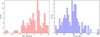 |
Fig. 1 Properties of the sample of polars with two-minute time-resolution TESS light curves. Left panel: histogram of TESS magnitudes. Right panel: histogram of distances (from Bailer-Jones et al. 2021). |
2 Master catalogue of polars
This article is based on a comprehensive catalogue of polars that we compiled from the literature. The full catalogue of polars is the subject of a separate publication (Schwope 2025). The list of polars continuously evolves, and we used the preliminary version of the catalogue compiled up to Summer 2024. This catalogue comprises 217 systems. It serves as the input list for our systematic search for rotation periods in TESS data.
The catalogue of polars comprises orbital periods that were obtained from a meticulous literature study and which serve in the context of this work to validate the periods that we detect with TESS.
We adopted the Gaia DR3 source IDs (Gaia Collaboration 2023), hereafter Gaia DR3 IDs, provided by Schwope (2025), for all systems except for 2XMM J154305.5-522709. For this system, a TESS two-minute cadence light curve is available (see Sect. 3), but no Gaia DR3 ID is given in Schwope (2025). Therefore, we used the J2000 equatorial coordinates to perform a cross-match in TOPCAT (Taylor 2005) and retrieve its Gaia DR3 ID. For all systems, the Gaia DR3 photometry was subsequently acquired through the Gaia Archive1.
3 TESS database
TESS is a NASA space-based mission led by MIT. Initially designed to conduct an almost full-sky survey (excluding the ecliptic plane) over two years, the mission has been extended and continues to re-observe the sky, now entering its additional sixth year beyond the original timeline. The observational strategy of TESS divides the sky into sectors, each covered for two consecutive satellite orbits (~27 days). In the mission’s first year (2018–2019), the southern ecliptic hemisphere was observed, followed by the northern ecliptic hemisphere in the second year (2019–2020). In its extended mission, TESS continues its sector-based sky survey with expanded target lists and additional coverage of the ecliptic plane. As of February 2025, TESS has completed observations through sector89.
In this work we use data from Sectors 1 to 63. First, we performed a cross-match within TOPCAT using the J2000 equatorial coordinates. This way, we retrieved the unique identifiers of our targets in the TESS Input Catalogue (Paegert et al. 2022), hereafter referred to as TIC IDs, and their TESS magnitudes. Then we searched in the Barbara A. Mikulski Archive for Space Telescopes (MAST)2 for two-minute cadence data of the 217 polars from our catalogue. We found that 95 of them have two-minute cadence data from at least one of the sectors (within Sectors 1–63). Many of our targets have several TESS two-minute cadence light curves from sectors corresponding to different years of observation or from sectors observed directly one after each other if the star is in the overlapping sky area of the two sectors. For each system in our sample we analysed all two-minute cadence light curves available from Sector 1–63.
The distributions of TESS magnitudes and distances from Bailer-Jones et al. (2021) for our sample are shown in the left and right panels of Fig. 1, respectively. We analysed the light curves with the PreSearch Data Conditioning Simple Aperture Photometry (PDCSAP) fluxes, which is the pipeline-corrected version of the photometric fluxes that mitigates instrumental effects. The journal of observations, combined with the data table for our results from the period analysis, is available electronically at CDS (see Table A.1 for details about the content).
4 Search for orbital periods
4.1 Data preprocessing
As a first step, we removed data points with TESS quality flags different from zero, ensuring that unreliable or flagged measurements are excluded from the analysis.
TESS light curves contain gaps of ~1−2 days, the Low Altitude Housekeeping Operations (LAHO) gaps, used for data transfer to Earth or, occasionally, due to technical problems. These discontinuities are potentially problematic for our analysis, impeding some algorithms to work properly. Therefore, we performed a linear interpolation across all gaps – both those associated with LAHO and missing points associated with problematic quality flags – between the last observed point before each gap and the first observed point after it.
To assess whether the linear interpolation biases the period estimation, we compared the period estimates using the Lomb-Scargle periodogram on our sample with and without applying linear interpolation. The results showed a mean percentage difference of 0.020% and a maximum difference of 0.098%, both values within the typical noise uncertainties. Thus, we conclude that the linear interpolation does not significantly bias the period determination.
Nevertheless, the interpolated light curves were only used for the autocorrelation function (ACF) and Fourier power spectrum methods, for which uninterrupted data is required. No interpolation was applied when using the Lomb-Scargle periodogram or sine fitting methods (see Sect. 4.2).
Finally, we normalised the light curves by the mean value of the photometric flux.
4.2 Detection methods
For the detection of orbital periods from TESS light curves, four numerical methods are employed: Lomb-Scargle periodogram, the autocorrelation function, sine fitting, and Fourier power spectrum analysis. Utilising multiple methods ensures robust and accurate period determination by mitigating biases inherent to individual techniques, uncovering subtle periodic signals that could be missed by individual methods alone and allowing cross-validation of the different period estimations.
The Lomb–Scargle periodogram (Lomb 1976; Scargle 1982) is an algorithm especially suitable for detecting periodic signals in unevenly sampled time series. The autocorrelation function measures the similarity between the observed light curve and a delayed version of itself revealing periodic patterns. The autocorrelation coefficient is computed at different time lags. A fast Fourier transform (FFT) (Cooley & Tukey 1965) is then applied to the obtained autocorrelation coefficients, allowing the identification of the periodic signals that are present in the light curve. Sine fitting is performed using non-linear least squares using the Levenberg-Marquardt algorithm (Levenberg 1944). Finally, a Fourier power spectrum with Kaiser windowing (Kaiser & Schafer 1980) is obtained for each light curve using a beta parameter β = 3. The Kaiser window provides an important flexibility in trading off the main lobe width and the sidelobe levels by adjusting the beta parameter. With β = 3, the Kaiser window achieves a good compromise between suppressing side-lobes sufficiently and maintaining a good frequency resolution. The software routines used in this work are based on Python implementations available in the statsmodels, Astropy, and Scipy packages.
4.3 Results
With the analysis described in Sect. 4.2 we obtain one period measurement per method per light curve, and given that some systems were observed in two-minute cadence throughout Nsec different sectors, the number of period values we obtain for a given star is up to 4 × Nsec. To determine the final adopted period for each system, we first compute sector-averaged periods for each period search method, that is, 〈Porb,LS〉, 〈Porb,ACF〉, 〈Porb,SINE〉, 〈Porb,FS〉; see description in Sect. 4.6. This approach allows us to evaluate the performance of the different period search methods and to discard possible systematic effects. However, no systematic trends between the period values found with the different methods are observed.
The use of multiple period detection methods and the availability of several light curves per star require to set up a procedure for the determination of the final adopted orbital period, Porb,final, of each star. We explain our approach in Sects. 4.4–4.6, including the treatment of the uncertainties, the correction of modulations at 1/2 Porb and the procedure for determining the final adopted periods.
To validate our new period detections, we visually inspected the Lomb-Scargle periodogram, ACF, and Fourier power spectrum plots for each light curve. Additionally, for each system in which a period could be measured from the TESS data, a comparison of Porb,flnal against values previously reported in the literature was carried out and the measurements that deviate most from the earlier literature value for the same star were flagged. Hereby, we use the most recent literature reference and value. We performed this cross-check by first calculating the difference between the literature period and the final adopted period, Porb,final, for each system, Pdif = Porb,lit − Porb,final. Then, we computed the 95th percentile of the absolute values of all Pdif values. All period measurements, Porb,final, for which |Pdif | is smaller than this threshold were then deemed consistent with the literature value.
Out of the 95 systems analysed, we were able to measure an orbital period for 93 systems. Among these, for 85 systems the measured orbital periods are consistent with the values reported in the literature. The sample studied also comprises four asynchronous systems which are analysed in detail in Sect. 4.6.1. For four systems, the measured orbital periods were not consistent with values reported in the literature. In these cases, a careful examination was performed that is explained in Sect. 4.6.2. Additionally, for two systems, the presence of noise in their TESS light curves impeded a period measurement (Sect. 4.6.3).
In an electronic table available at CDS (see Table A.1), all the studied 95 polars are presented together with the orbital periods Porb,final measured from their TESS two-minute cadence light curves and their uncertainties (explained in Sect. 4.4). We also provide the literature reference for the previously reported value of the orbital period Plit.
4.4 Uncertainties
Quantifying the uncertainties associated with the periods detected in light curves is notoriously challenging. In this context, common practice consists in measuring the width of the periodogram peak associated with the orbital period (see e.g. Mennickent et al. 2003 or Nagel et al. 2016). The uncertainty is then directly ascribed to the half-width at half-maximum in the frequency peak or the standard deviation obtained from a Gaussian fit to the frequency peak. However, this methodology is conceptually limited, as the width of the frequency peak is a naive estimation of the precision associated with a period measurement, ignoring factors such as the noise in the data.
The reason is that these uncertainty estimates are intrinsically linked to the frequency resolution. In a Fourier transform, the frequency resolution is the inverse of the total observation time of the time-series data. In the discrete Fourier transform: ∆ƒ = 1/(N∆t), where N is the number of data points and ∆t is the time-resolution. Thus, given a fixed total observation time of the time-series data, the frequency resolution and, consequently, the width of the frequency peak in the periodogram, are, to a first order approximation, independent of both the sampling cadence and the S/N of the data points. In addition, the frequency width is highly dependent on how the periodogram is obtained. The use of different window functions can drastically change the obtained main lobe widths of the frequency peaks (see VanderPlas 2018 for a detailed discussion).
Hence, this methodology measures the precision associated with the limited frequency resolution, which depends on the total observation time of the time-series data and not on the quality of the data, misconceiving the true variability in the detection process. Instead, it is more appropriate to estimate the uncertainty associated with the statistical variations, due to factors such as noise, instrumental systematics, and errors introduced by the period-search methods.
Thus, we made use of the multi-epoch data of our targets. Forty-three of the systems have more than one two-minute cadence TESS light curve. For these cases, we computed the uncertainty in the period on a per-method basis by calculating the 1σ confidence interval for the sample of periods retrieved with a given period-search method, as described in Sect. 4.6. We note that this approach is generally applicable for polars, whose orbital periods remain stable over long timescales (typically decades or longer; see e.g. Applegate & Patterson 1987 and Applegate 1992). For other types of variable stars, however, additional diagnostics may be necessary to ensure that the observed scatter in period estimates from different epochs is not due to evolutionary effects or episodic events like outbursts.
For the 52 systems with only one two-minute cadence TESS light curve, the uncertainties in the detected periods were estimated using a Monte Carlo resampling approach. Hereby, each Monte Carlo realisation of the observed light curve is produced by (1) adding noise drawn from a normal distribution with zero mean and a standard deviation equal to the photometric uncertainties of the original flux measurements, and (2) applying a resampling with replacement to the time–flux pairs, that is, time–flux pairs are randomly drawn from the original time-flux measurements, where replacement means that some time-flux pairs can be selected multiple times while others may be omitted. This procedure is repeated 1000 times and for each simulated light curve, the Lomb-Scargle periodogram is computed over a narrow frequency range centred on the originally detected frequency. Specifically, we used a frequency grid spanning ±10% around the detected frequency peak. The distribution of the resulting dominant frequencies is cleaned using an iterative 3-σ clipping procedure to remove outliers. In this process, values exceeding 3 standard deviations from the median are removed, after which the median and standard deviation are recalculated. This step is repeated until no further outliers are identified, leading to a Gaussian-like distribution. The frequency uncertainty is then estimated from the standard deviation of this distribution.
While this method captures the effects of random noise and sampling variability, we note that it may underestimate the full uncertainty associated with the period determination. For example, in each realisation of the observed light curve, it is assumed that the observational noise is purely white, that is uncorrelated, whereas in reality, different realisations of red noise can also affect the period determination. In addition, the LAHO gap in the observed TESS light curve is kept fixed in both position and duration across all Monte Carlo realisations, which neglects its potential impact in biasing the period determination. Finally, any instrumental systematics present in the original light curve are approximately preserved in all simulated realisations of the observed light curve, potentially biasing the resulting distribution of dominant frequencies.
4.5 Periods at 1/2 Porb
During our search for orbital periods, dominant modulations in the light curves at half the period reported in the previous literature were encountered in 38 systems. If we assume that the literature values correspond to the orbital period, our measurements for these 38 systems represent half the orbital period (1/2 Porb). The detection of orbital periods in polars, indeed, underlies ambiguities because various physical processes may cause periodicities at one half of the orbital cycle. These phenomena are here briefly discussed before we explain how we mitigated wrong values of Porb due to their presence.
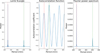 |
Fig. 2 Illustration of the results from different period detection methods for a case where the dominant period is 1 /2 Porb (from left to right): Lomb-Scargle periodogram, ACF, and Fourier power spectrum. The example refers to TIC 124404442 (alias V1043 Cen) (sector 37). The red vertical lines indicate the signals at 1/2 Porb, while the green vertical lines indicate the true orbital period (Sparks & Sion 2021). In this light curve, all three methods failed to identify the orbital period. We note that although the autocorrelation coefficient at the true orbital period is higher than that at 1/2 Porb in the ACF plot, the subsequent FFT applied to the autocorrelation coefficients yields a stronger signal in 1/2 Porb. |
4.5.1 Physical mechanisms producing periods at 1/2 Porb
A primary cause of periodic light curve patterns at 1/2 Porb is accretion to both magnetic poles of the white dwarf (see e.g. Ferrario et al. 1989 and Ok & Schwope 2022). When accretion occurs at both magnetic poles, a distinct hotspot is produced at both polar regions. These spots contribute to the overall brightness of the system. Depending on the inclination angle, as the binary system orbits, these hotspots come in and out of view and give rise to a periodic modulation of the observed brightness. For appropriate inclinations the observer might see two maxima per orbital cycle, one from each magnetic pole, and a periodic signal corresponding to half the orbital period of the binary system will be detected.
The accreting region of the white dwarf can be the source of significant cyclotron emission due to the strong magnetic field of the white dwarf (see Schwope 1990). Cyclotron beaming combined with a misalignment between rotation and magnetic axis (that is a non-zero colatitude angle β) appears, thus, as another potential source of brightness modulations at 1/2 Porb in light curves of polars. Cyclotron beaming is highly anisotropic and the emission is channelled along a direction approximately perpendicular to the magnetic axis. For β ≠ 0 and inclination angle i ≠ 0, the hotspot, located near the accreting magnetic pole, will produce cyclotron beaming that changes its orientation as the white dwarf rotates moving into and out of the observer’s view. The variation in the orientation of the beamed radiation relative to the observer’s line-of-sight leads to a periodic modulation of the observed brightness – with a typical amplitude of ~1 mag (see e.g. Vogel, J. et al. 2007) – which has a period of half the orbital period, since each complete rotation of the white dwarf results in two instances where the cyclotron beam is directed towards the observer.
Another possible cause of signals at 1/2 Porb is ellipsoidal modulation. In CVs, the donor becomes distorted into an ellipsoid due to the strong gravitational influence of its close WD companion. This distortion causes periodic brightness variations – typically with amplitudes of 0.01–0.2 mag – as the projected surface area of the elongated star changes during the orbit (see e.g. Wilson 2006 and Bochkarev et al. 1979). Generally, the same modulation pattern repeats twice per orbital period since the ellipsoid presents similar cross-sectional areas twice per orbit. This leads to a contribution to the light curve that exhibits two maxima and two minima per orbital period.
4.5.2 Results for our sample
The identification of periods in the TESS light curves that represent 1/2 Porb was primarily done by comparison with previously reported values from the literature, which were taken as a reference for the orbital period of the systems. In addition, we searched for a signal at twice the measured value to double-check if the dominant observed period is, indeed, 1/2 Porb. If the detection that corresponds to the strongest signal in the light curve is half the orbital period, the signal corresponding to the actual orbital period should, in principle, also be present. Specifically, the Lomb-Scargle periodogram and the Fourier power spectrum should present two frequency peaks at the positions corresponding to Porb and 1/2 Porb. The ACF should exhibit two superposed periodic modulations. An example of such a case is illustrated in Fig. 2.
The search for two periodic signals that differ by a factor two is particularly useful when applied to new samples of CV candidates without previously reported periods in the literature, providing a systematic way to verify whether the detected signal corresponds to half the true orbital period. Additionally, we recommend inspecting the phase-folded light curves for both the detected period and the possible true period at twice the period with the strongest signal. The light curve folded with 1/2 Porb shows the superposition of two different modulations, at 1/2 Porb and at Porb, typically with different amplitudes. The light curve folded with the true orbital period reveals these two modulations and aligns with other periodic phenomena, such as eclipses. An example illustrating these differences is shown in Fig. 3.
Out of the 93 systems for which a period was detected, we identified 38 systems where some of the detections actually represent 1/2 Porb. For some systems, different light curves yielded a different dominant periodicity, either 1/2 Porb or Porb. More-over, in some instances, for a specific light curve, one numerical method identified 1/2 Porb as the strongest signal, while another method favoured Porb as the dominant modulation. For all the independent detections corresponding to 1/2 Porb, the difference between the literature values and twice the detected periods is on the order of seconds or less, which is within the noise error. These values were, thus, corrected by simply taking the double of the detected period Pdet, that is the corrected period is Pcorr := 2Pdet. We note that, in general, doubling a noisy period estimate may misidentify Porb. However, in our study, no cases were encountered where the dominant periodicity at 1 /2 Porb was noisy. In the table available at CDS (see Table A.1), we provide a flag for the systems where at least one of the individual measurements involved in calculating the period we report has been corrected this way.
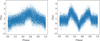 |
Fig. 3 Phase plots for the light curve of TIC 258799357 (alias EP Dra) (sector 26), an eclipsing polar, as an example of a light curve where the dominating modulation is at 1/2 Porb. Left panel: light curve folded over the detection at 1/2 Porb. Right panel: light curve folded over the true orbital period (Schwope & Mengel 1997). The true orbital period (right panel) displays the pattern corresponding to one complete orbit of the primary star around the secondary, with the eclipse distinctly visible around phase 0.5. |
4.6 Determination of final adopted orbital period values
As mentioned in Sect. 4.3, since the same object may have been observed in Nsec different sectors, and for each light curve we measure the orbital period from four different numerical methods, for a given system we obtain up to 4 × Nsec period values. We note that not for all light curves, a period was found with all detection methods. Conversely, for a given system, a particular detection method may not find a period in all the available light curves. The following procedure was implemented to determine the final values for the orbital periods and their uncertainties.
First, all pathological detections were identified and discarded. This identification of erroneous detections was clear in many cases, where the detected periodicities were several orders of magnitude higher than the expected orbital periods for CVs, Porb,CVs ~ 80–360 min (see e.g. Knigge 2011) and the longest observed orbital period for a polar (V1309 Ori with 478.96 min; Sparks & Sion 2021).
In these cases, the detection failed in finding the correct periodic signal due to factors such as the predominance of instrumental artefacts or noise. For instances where a spurious detection was obtained initially, the period search methods were reapplied with the search range restricted to 30–1000 minutes. This range extends beyond the typical range of orbital periods for CVs to encompass both the typical orbital periods of CVs and possible outliers, while still allowing the recovery of signals that may have been missed in the initial attempt, particularly due to the presence of dominant low-frequency power from red noise.
Detections within the expected range of orbital periods in CVs, but not in accordance with the literature reference, were subjected to further study as follows.
When a detected period value is in disagreement with other measurements, that is, detections made by other numerical methods or in other observed TESS light curves (if they exist), and those other measurements align with the literature value, an individual inspection of the measurement was done to confirm whether it constituted a faulty detection, for example whether the measured period arose from noise. In practice, in all these cases, the deviating period was discarded. If no additional detection in agreement with the literature value was made from the TESS light curves and it is not clear if the detection was faulty, the deviating measurement was retained and a detailed analysis was done on an individual basis in order to assess if the identified signal could correspond to the orbital period. These cases are discussed in Sects. 4.6.1 and 4.6.2.
Once the pathological cases were disregarded and the periods corresponding to 1/2 Porb were identified and corrected (see Sect. 4.5.2), the final adopted orbital period values were calculated. For those systems which were repeatedly observed, that is, systems for which there exist several observed two-minute cadence TESS light curves, final values of the orbital period were computed for each detection method by taking the average among all repeated observations,
 (1)
(1)
Here Porb,k,j is the orbital period for the method k (accounting for Lomb-Scargle periodogram, the autocorrelation function, sine fitting, and Fourier power spectrum analysis) and the observed light curve j, nk is the total number of detections in different observed light curves with the detection method k, and Porb,k is the orbital period associated with a specific detection method k. As mentioned above, a given detection method may fail to detect a period in some light curves, that is, nk ≤ nobs, where nobs is the number of available two-minute cadence TESS light curves of the system.
The uncertainties were calculated as the 1σ confidence interval of the different period measurements using the standard error scaled by the appropriate Student’s t-factor. This was done separately for each of the four implemented period search methods, thus, providing an estimate of the uncertainty for each numerical method,
 (2)
(2)
where ΔPorb,k is the orbital period uncertainty associated to a specific detection method k, σ denotes the standard deviation, and ***(eq3)*** is the two-tailed critical value of the Student’s t-distribution for a confidence level of 68.27% and nk − 1 degrees of freedom. If for a numerical method k, only one measurement exists, that is, nk = 1, the standard deviation is not defined, and therefore no uncertainty ΔPorb,k was associated to that numerical method.
After associating for a given target a unique orbital period and, if possible, an uncertainty to each detection method, the final adopted orbital period and its uncertainty are selected as the pair with the lowest relative uncertainty,
 (3)
(3)
which corresponds to adopting the most precise estimate among the implemented methods.
For systems with only one available two-minute cadence TESS light curve, the final orbital period is adopted from the Lomb-Scargle periodogram. In these cases, the uncertainty is estimated using a Monte Carlo approach, as described in Sect. 4.4. In the following, we discuss the 10 systems where Porb,final is inconsistent with the literature value.
Orbital and spin periods of asynchronous systems in the sample of polars observed with TESS in two-minute cadence.
4.6.1 Asynchronous systems
In some polars, the spin period of the WD is not synchronised with the orbital period, leading to complex light curve variations. For some of these asynchronous systems, the spin period signal (hereafter denoted as the frequency ***(eq5)*** ) can be more prominent than the orbital period (hereafter denoted as the frequency ***(eq6)***
 ), and this may lead to wrong interpretations of the detected periodic signal. Additionally, the mismatch between the WD’s spin and the orbital motion causes drifting of the accretion spots across the WD’s surface and ‘pole-switching’ accretion, that is, the accretion channel ends alternately on the two poles of the WD. This is because in discless CVs the accretion stream feeds material along the WD’s magnetic field lines onto the closest magnetic pole. Since the secondary star and the stream co-rotate with Ω, the WD’s dipole field rotates at an apparent angular frequency ω − Ω, as seen in a frame co-rotating with the binary’s orbital motion at frequency Ω. Consequently, as the phase difference between ω and Ω evolves in time, accretion alternates between the two magnetic poles. To a first approximation, the ‘pole-switching’ phenomenon occurs when the spin and orbital phase differ by 90º. This causes a brightness modulation at the beat period 2π (ω − Ω)−1, as each magnetic pole is actively accreting for half this beat period. Additional considerations about the system’s geometry explain the modulations at additional beat frequencies (e.g. 2ω − 3Ω, 2ω − Ω, 4ω − 3Ω) between ω and Ω, also denominated as side-band frequencies (see Wynn & King 1992; Wang et al. 2020 and Sobolev et al. 2021 for a detailed description).
The sample studied in this work comprises four systems that display such asynchronous rotation. For these cases, a deeper analysis of their Lomb-Scargle periodograms was performed to distinguish between the spin period and the orbital period. In Table 1, the orbital and spin periods measured in these systems are summarised. Additionally, all detected periodicities, together with their interpretations and S/NPSD values (see Appendix E), are reported in Tables B.1–B.4 in Appendix B. As discussed in Sect. 6, period detections with S/NPSD < 0.004 are considered highly unreliable. In the following, we describe these measurements in detail and we compare them to the results from previous studies of the same systems.
BY Cam (TIC 339374052). Several periods were found for this system in previous observations (see e.g. Mason et al. 2022 and references therein). The asynchronous rotation of the primary leads to brightness modulations at Ω, ω, and additional beat frequencies. The side-band frequency at 2ω − Ω is typically the most dominant signal and has been detected in multiple occasions for BY Cam (Silber et al. 1997; Mason et al. 1998; Pavlenko et al. 2013; Honeycutt & Kafka 2005, and Mason et al. 2022).
In our study, two TESS light curves were analysed, corresponding to sectors 19 and 59 (see Fig. 4).We detect signals corresponding to the orbital and spin periods, as well as the side-band period 2π (2ω − Ω)−1. Additionally, we identify multiple periodicities that we associate with side-band periods and their harmonics. Among all the detected signals, only the periods P8, P9, P10, P11, P13, and P18 have been previously reported (see Mason et al. 1998; Honeycutt & Kafka 2005; and Mason et al. 2022). Our results are presented in Table B.1. With the adopted interpretation of the different periods, we follow Mason et al. (2022), in which the interpretation of the spin period is based on X-ray and polarisation analyses (see Mason et al. 1989 and Mason et al. 1998) and the interpretation of the orbital period is based on spectroscopic studies (see Mason et al. 1996 and Schwarz et al. 2005).
IGR J19552+0044 (TIC 228975750). Tovmassian et al. (2017) determined a period Pspin = 81.3 min using ground-based multi-band timeseries photometry and a period Porb = 83.6 min from ground-based optical spectroscopy.
In our work, the sector54 TESS light curve of IGR J19552+0044 revealed a distinct frequency peak at 81.3011 ± 0.0015 min and a smaller signal at 83.0153 ± 0.0086 min, corresponding to the periods P4 and P5 in the bottom panel of Fig. 5, respectively. Consistent with the findings of Tovmassian et al. (2017), we identify the first signal with the spin period, Pspin = 81.3011 ± 0.0015 min, whereas the second is tentatively ascribed to the orbital period, Porb = 83.0153 ± 0.0086min. However, given the low significance of this frequency peak, its presence is questionable.
We find four additional low-power signals (see Fig. 5 and Table B.2) that have not been reported in the previous literature. We interpret the periodicites P1 and P2 as half the spin period and half the orbital period, respectively. Tovmassian et al. (2017) found that the amplitude of the photometric variability was wavelength-dependent. Along with the changing shape of the system’s spectral continuum, this was regarded as evidence of cyclotron radiation. Following this interpretation, we assume that the variability at the spin period originates from cyclotron radiation emitted by the magnetic white dwarf, naturally explaining the signal at 1/2 Pspin (see Sect. 4.5.1). The signal at half the orbital period is likely due to ellipsoidal modulation. The other two periods, P3 and P6, are interpreted as the side-band periods 2π (4ω − 3Ω)−1 and 2π (3Ω − 2ω)−1, respectively (see Table B.2).
CD Ind (TIC 231666244). Littlefield et al. (2019) found three significant periods in the TESS sector 1 light curve: a period Porb = 112 min interpreted as the orbital period, a period Pspin = 110.8 min interpreted as the spin period, and a period 2π(2ω − Ω)−1 = 109.6 min interpreted as a side-band period. Additionally, their analysis revealed multiple side-band periods and its harmonics in the power spectrum.
In this work, we analysed two TESS light curves corresponding to sectors 1 and 27. We confirm the periods found by Littlefield et al. (2019) in sector 1 and present the periods identified in sector 27 (see Fig. 6 and Table B.3). The adopted interpretation of the orbital and spin periods follows Littlefield et al. (2019). Many of the periods observed in sector 1, are also identified in sector 27. The detection of these periods in independent light curves further supports its physical origin and allows a more precise determination of their values. In sector 27, the side-band period 2π (2ω − Ω)−1 (labelled P9) appears with higher significance, while other side-band periods are less prominent. Notably, the periods P2, P5, P10, P11, and P17 are not present in sector 27 (see Fig. 6). The absence of P10 and P11 is particularly relevant, as they correspond to the spin and orbital periods, respectively. In addition, the side-band P12, which is not clearly present in sector 1, appears with greater significance in sector 27.
Paloma (TIC 369210348). Schwarz et al. (2007) proposed two different period identifications which were later verified by Littlefield et al. (2023) using TESS data. According to the interpretation given by these latter authors, the spin period of the white dwarf is 136.2 min and the orbital period is 157.2 min.
We re-analysed the same TESS sector 19 light curve and confirmed the periods found by Littlefield et al. (2023). Here, we present the most significant periods (see Fig. 7 and Table B.4).
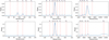 |
Fig. 4 Zoomed-in view of the Lomb-Scargle periodograms of the TESS light curves of TIC 339374052 (alias BY Cam). Top panels: Sector 19. Bottom panels: Sector 59. The red lines mark the positions of the different periodicities that were measured (see Table B.1). |
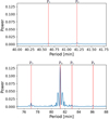 |
Fig. 5 Zoomed-in view of the Lomb-Scargle periodogram of the TESS light curve of TIC 228975750 (alias IGR J19552+0044) (sector 54). The red lines mark the positions of the different periods that were measured (see Table B.2). |
4.6.2 Outliers
Among the 95 polars analysed, for four systems the orbital periods detected with TESS exhibit values that deviate significantly from values reported in the literature, as determined by their period differences exceeding the 95th percentile threshold (see Sect. 4.3). Here each of these outliers is examined individually.
2XMM J154305.5-522709 (TIC 1140118632). van den Berg et al. (2012) reported two periods based on Chandra X-ray data: P1 = 73.2 ± 4.83 min and P2 = 146.2 ± 15.95 min. Servillat et al. (2012) reported a period of 143.4 min based on multi-epoch K-band photometry, which appears consistent with the longer of the X-ray periods in van den Berg et al. (2012). However, given the highly incomplete sampling of the infrared (IR) light curve, the reliability of this period in the IR data is questionable.
In this work, a frequency peak corresponding to a period of 144.6 min is observed in the Lomb-Scargle periodogram of the only available two-minute cadence TESS light curve (sector 39), but its distinction from noise is doubtful (see Fig. 8). A dominant frequency peak is located at 260.90 ± 0.29 min (see Fig. 8). Notably, the same periodicity is detected by all four implemented period search methods. It is possible that this modulation was not found by van den Berg et al. (2012) because their X-ray light curve spans only ~500 min.
This object is located in a crowded field along the Galactic plane. Therefore, we assessed the possibility of contamination by neighbouring astrophysical objects contributing to the flux in the TESS light curve. Hereby, the methodology from Binks et al. (2022) was followed. Briefly, all Gaia sources within a certain pixel radius of the target are considered and the contribution from these sources to the circular target aperture is given by (see Biser & Millman 1965),
![Mathematical equation: ${f_{{\rm{bg}}}} = \sum\limits_i {{{10}^{ - 0.4{G_i}}}} \,{e^{ - {t_i}}}\sum\limits_{n = 0}^{n \to \infty } {\left\{ {{{t_i^n} \over {n!}}\left[ {1 - {e^{ - s}}\sum\limits_{k = 0}^n {{{{S^k}} \over {k!}}} } \right]} \right\}} ,$](/articles/aa/full_html/2025/11/aa54948-25/aa54948-25-eq7.png) (4)
(4)
where the outer summation includes all potential contaminant sources, G represents the G-magnitude, s = R2/2σ2, t = D2/2σ2, R is the radius of the aperture in pixels, D is the distance between the potential contaminating object and the centre of the target aperture in pixels, and σ is the full width at half-maximum of the TESS point spread function, which is roughly 0.65 pixels.
The contaminating flux, ƒbg, is then compared with the flux from the target object within the aperture radius. The latter is approximately given by a Rayleigh distribution,
 (5)
(5)
Considering an aperture radius of three pixels (63 arcsec), we find that the strongest contaminating source contributes with a flux of 2.12 × 10⁻⁵ and the total background contribution is ƒbg ≈ 2.62 × 10⁻⁵. The target’s flux is ƒ* ≈ 8.27 × 10⁻⁸, yielding a contamination ratio of ƒbg/ ƒ* ≈ 3.17 × 10². With such a high contamination ratio, the possibility that the periodic signal in the TESS light curve arises from contamination of a neighbouring source cannot be discarded. On the other hand, none of the known objects within a two-arcmin radius is of a type for which a period of 260 min can be expected.
Since the X-ray light curve presented by van den Berg et al. (2012) shows a clear periodic behaviour, the interpretation given here is that the correct orbital period is Porb = 146.2 min from van den Berg et al. (2012). In our analysis of the TESS light curve, we find a period of 260.90 ± 0.29 min; however, due to the high contamination ratio it remains highly unreliable and such that follow-up studies are suggested.
GQ Mus (TIC 908535248). Diaz & Steiner (1989) reported a period of 85.5 ± 0.4 min based on data obtained with a photometer at the 1.6 m telescope of the Laboratório Nacional de Astrofísica at Brasópolis MG, Brazil. In our study, two TESS light curves were analysed, corresponding to sectors 37 and 38. Different periods are found in the two light curves, namely P1 = 249.64 ± 0.57 min in sector 37 (see top panels in Fig. 9) and P2 = 495.1 ± 2.3 min in sector 38 (see bottom panels in Fig. 9). No significant frequency peaks near 85 min were detected. The two periods detected are roughly distinguished by a factor two (where P1 is ~4 min different to 1 /2 P2), suggesting that the periods could be physical. However, both light curves present high levels of noise. Therefore, it cannot be excluded that these detections are spurious. As a matter of fact, GQ Mus has a TESS magnitude of 18.796, and in Sect. 6.2 we argue that for TESS magnitudes ≥17 a substantial number of light curves are too noisy to reliably determine the orbital period. In fact, as shown in Fig. 15 which is discussed in Sect. 6.2, the periodic signals detected in the TESS light curves of GQ Mus present a S/NPSD (see Appendix E) below the limiting value for a reliable orbital period detection. Thus, follow-up observations are required to confirm the orbital period for this system.
J0733+2619 (TIC 94840820). Denisenko et al. (2011) identified two potential orbital periods based on Catalina Real-Time Transient Survey (CRTS) optical light curves: P1 = 192.1 min and P2 = 200.9 min. Gabdeev (2015) reported an orbital period of 200.29680 ± 0.00029 min based on photometric observations performed with the 1m Zeiss-1000 telescope of the Special Astrophysical Observatory of the Russian Academy of Sciences (SAO RAS), which aligns with the longer period reported by Denisenko et al. (2011).
We studied three TESS light curves, corresponding to 44,45, and46. All three light curves present long term non-linear trends, likely driven by instrumental effects, that dominate the observed variability. For this reason, Lomb-Scargle periodograms were generated with a frequency range restricted to 0–1000 minutes. The ~200.8 min period from Denisenko et al. (2011) is recovered with high significance in all three light curves (see Fig. 10). Following the procedure described in Sect. 4.6, our final adopted orbital period value is Porb = 200.79 ± 0.13min. The period at 192 min claimed by Denisenko et al. (2011) is not observed in the TESS light curves. Due to the much poorer data sampling of the CRTS visual light curves compared to the TESS light curves, our value for the (orbital) period measured on TESS data should be considered as more reliable; moreover, we are able to provide an uncertainty on this measurement based on multiple detections of the periodicity. The orbital period reported by Gabdeev (2015), although not formally consistent with our result within the uncertainties, is in close agreement, further supporting the reliability of its detection.
J1424-0227 (TIC 1002329407). Harrison & Campbell (2015) reported a period of 230.4min based on WISE data. Additionally, Marsh et al. (2002) reported a period of 223.92min using the ISIS spectrograph on the 4.2 m William Herschel Telescope in the Canary Islands. Our analysis of the TESS light curve for J1424-0227(sector51)revealedaperiodof121.636±0.063min (see Fig. 11). However, the TESS light curve is noisy and it contains two data gaps in addition to the LAHO gap.
The high noise level in the TESS light curve can be explained by the faintness of the system, which has a TESS magnitude of 17.541, in the range where according to our analysis a period detection is potentially unreliable (see Sect. 6.2). Under these circumstances, it becomes difficult to assess if the signal at 121 min has a physical origin. Considering that signals at ~230 or ~223 min are not present in the TESS light curve, we suggest follow-up observations to confirm the orbital period.
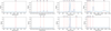 |
Fig. 6 Zoomed-in view of the Lomb-Scargle periodograms of the TESS light curves of TIC 231666244 (alias CD Ind). Top panels: Sector 1. Bottom panels: Sector 27. The red lines mark the positions of the different periods that were measured (see Table B.3). |
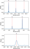 |
Fig. 7 Zoomed-in view of the Lomb-Scargle periodogram of the TESS light curve of TIC 369210348 (alias Paloma) (sector 19). The red lines mark the positions of the different periods that were measured (see Table B.4). |
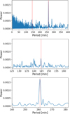 |
Fig. 8 Top panel: Lomb-Scargle periodogram of the two-minute cadence TESS light curve of TIC 1140118632 (alias 2XMM J154305.5-522709) (sector 39). Centre panel: zoomed-in view of the frequency peak located at 144.6 min. Bottom panel: zoomed-in view of the frequency peak located at 260.90 ± 0.29 min. The red lines mark the positions of the frequency peaks. |
4.6.3 Unsuccessful period measurements
For two systems, J0257+3337 (TIC 641322558) and V379 Vir (TIC 953321496), the S/N of their two-minute cadence TESS light curves did not allow us to recover the (orbital) periods previously reported by Vladimirov et al. (2014) and Stelzer et al. (2017). Fig. 12 shows their corresponding Lomb-Scargle periodograms. It is important to note that J0257+3337 and V379 Vir have TESS magnitudes of 18.18 and 17.99, respectively. This is in accordance with our results presented in Sect. 6.2, where we establish that for TESS magnitudes ≥17 mag, period detections are highly unreliable.
5 Flattened light curves
To determine the correlation between the noise levels in the studied light curves and the TESS magnitude, the light curves were ‘flattened’ removing their periodic modulations, thus leaving only the noise as the content of the light curve.
The flattening methodology consists in generating smoothed versions of the observed light curves using the centred moving average algorithm (Hyndman 2011). To conduct this analysis, an interactive code was developed, which allowed the precise adjustment of the smoothing window size for each individual light curve, and therefore ensured an optimal smoothing. Excessive smoothing would impede a correct estimation of the astrophysical periodic modulation, causing significant details to be lost. Conversely, insufficient smoothing would additionally capture noise and fail to adequately filter out random fluctuations. The appropriate window size for each light curve was determined empirically through visual evaluation of the resulting smoothed light curves for different smoothing window values. In future works, this process could be automatised by selecting the smoothing window size that produces residuals with respect to the original light curve that best approximate a normal distribution.
By subtracting the smoothed light curves from the original observed light curves, one obtains the flattened light curves,
 (6)
(6)
Finally, once the flattened light curves are obtained, the standard deviation, Sflat, is computed. The standard deviation of flattened light curves, that is, light curves of which the (known) astrophysical signal(s) have been removed, serves as an estimation of the dispersion present in the noise. In Stelzer et al. (2016), we have introduced Sflat to characterise the noise in photometric light curves of M dwarf stars. Here the astrophysical signal that was removed to obtain flat light curves are rotational modulations due to star spots and flares. We note that for the calculation of the parameter Sflat in the M dwarf light curves, another automated code was used (see Raetz et al. 2020).
In our previous work on nearby M dwarfs observed in the K2 mission, we observed a correlation between Sflat and the Kepler magnitude Kp of the stars (see Stelzer et al. 2016 and Raetz et al. 2020). An analogous study on TESS data was presented by Stelzer et al. (2022). In Fig. 13, we show the relation between Sflat and the TESS magnitude for our sample of polars (black) together with the results from Stelzer et al. (2022) (red). For both samples the value of Sflat displayed in the figure is the mean of the values measured on the different TESS light curves of a given star. Since these nearby M dwarfs are much brighter than the known polars we closed the gap between the two samples with 340 X-ray selected M dwarfs in the Southern Continuous Viewing Zone of TESS from Joseph et al. (2024) (blue). For this subsample, only a single two-minute cadence TESS light curve was analysed per object.
A clear relation over almost ten orders of magnitude with a well defined lower envelope is observed between the noise level of the flattened light curve and the brightness of the star. In Stelzer et al. (2016) and Raetz et al. (2020), it was observed that fast rotating M dwarfs (rotation periods Prot < 10 days) exhibit higher Sflat values than slow rotating stars (rotation periods Prot > 10 days). We attributed this to an additional underlying noise of astrophysical origin, such as unresolved mini-flares or mini-spots, for the fast rotators. Similarly, the light curves of polars are affected by flickering, a stochastic variability occurring on timescales from milliseconds to hours, which constitute an intrinsic source of astrophysical noise in polars (see e.g. Bruch 2021; Iłkiewicz et al. 2022 and Scaringi 2014). While the periodic modulation due to the hotspot is effectively subtracted in our flattening process, the flickering component remains, contributing to varying noise levels and likely accounting for the higher dispersion observed in the sample of polars in Fig. 13.
Our Sflat parameter shares the rough profile of its dependence on the T magnitude with the root mean square Combined Differential Photometric Precision (rmsCDPP) (Jenkins et al. 2010; Christiansen et al. 2012). Originally developed for the Kepler mission and later applied to TESS, the rmsCDPP parameter is optimised for the evaluation of the detectability of transit-like signals. In Fig. 13, we also include for all objects in the three samples the 2-hour rmsCDPP measurements that are provided as a pipeline product with the TESS light curve. For a given star, the values of rmsCDPP displayed in the figure represent the mean of the individual rmsCDPP measurements from the different TESS light curves.
An important difference between the rmsCDPP and Sflat is that the former is calculated as the root mean square of the residuals relative to an average flux within short time intervals (in this case two hours). This means that, for longer timescales, rmsCDPP averages out high-frequency noise. Moreover, in the calculation of rmsCDPP, the data is filtered to produce white noise, effectively whitening the time-correlated (red) noise. Thus, rmsCDPP measures the white noise in a light curve over a specific timescale, making it more suitable for evaluating the noise level in time-localised events such as transits. In contrast, Sflat captures the instantaneous scatter at each datapoint after removing the astrophysical periodic modulation(s), preserving both high-frequency and red noise in the flattened light curves. Therefore, it is better suited for assessing the overall noise level affecting period analysis. The contribution of high-frequency noise to the scatter measured by S flat, which is averaged out in the calculation of rmsCDPP, explains the systematically higher values compared to rmsCDPP. This is consistent with the idea that our flattened light curves still comprise astrophysical noise sources, possibly manifest in the form of high-frequency and red noise.
To quantify the lower envelope in Fig. 13, we divided the data into eight bins based on TESS magnitudes. Within each bin, we selected the Sflat values below the 25th percentile to represent the lower envelope of the distribution. These selected data points were then used to perform a second-order polynomial fit:
 (7)
(7)
Here a, b, and c are the fitted coefficients. The fitting was performed using the Levenberg-Marquardt algorithm and to estimate the uncertainties in the fitted parameters, a bootstrapping approach was followed. That is, the data was resampled with replacement obtaining a total 10 000 pseudo-samples, and the fitting procedure was repeated for each pseudo-sample to obtain a distribution for each coefficient. The standard deviation of these distributions was taken as the uncertainty in the corresponding parameter. The best-fit coefficients and their uncertainties are a = 0.01290 ± 0.0021, b = −0.047 ± 0.056, and c = 2.22 ± 0.38.
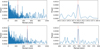 |
Fig. 9 Left panels: Lomb-Scargle periodograms of the TESS light curves of TIC 908535248 (alias GQ Mus) from Sector 37 (top) and Sector 38 (bottom). Right panels: zoomed-in view of the region around the highest frequency peaks, located at 249.64 ± 0.57 min (top for Sector 37) and at 495.1 ± 2.3 min (bottom for Sector 38). The red lines mark the positions of the frequency peaks. |
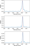 |
Fig. 10 Zoomed-in views of the frequency peak at ~ 200.8 min in the Lomb-Scargle periodograms of the TESS light curves of TIC 94840820 (alias J0733+2619). Top panel: Sector 44. Centre panel: Sector 45. Bottom panel: Sector 46. The red lines mark the positions of the frequency peaks. |
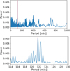 |
Fig. 11 Top panel: Lomb-Scargle periodogram of the TESS light curve of TIC 1002329407 (alias J1424-0227) (sector 51). Bottom panel: zoomed-in view of the frequency peak located at 121 .636 ± 0.063 min. The red lines mark the positions of the frequency peaks. |
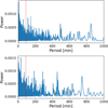 |
Fig. 12 Top panel: Lomb-Scargle periodogram for TIC 641322558 (sector 58). Bottom panel: Lomb-Scargle periodogram for TIC 953321496 (sector 46). The low S/N impedes the identification of periodic signals. The red lines mark the positions of the orbital periods reported in the literature (see Vladimirov et al. 2014 and Stelzer et al. 2017). |
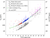 |
Fig. 13 Relation between Sflat and TESS magnitude for polars (pink) compared to the same relation for the M dwarf sample from Stelzer et al. (2022) (red) and a subsample of M dwarfs from Joseph et al. (2024) (blue). The TESS light curves of the latter were analysed by us (see Sect. 5). The lower envelope of the Sflat distribution (green dashed line) was obtained by fitting a second-order polynomial to the lower 25% quantile of the data. The two-hour rmsCDPP values for all objects in the three samples are presented for comparison (see Sect. 5 for details). |
6 Reliability of the detected periods
The detectability of orbital periods is significantly influenced by the S/N of the observed light curves. In this section, we describe the methodology and the results of an investigation aimed at determining the limiting S/N necessary for a reliable orbital period detection in TESS light curves of CVs. As specified in Appendix E, in this analysis, the S/N refers to the significance of that frequency peak in the power spectral density (PSD) of a light curve that is associated to the orbital period. In the following we denote this signal-to-noise ratio as S/NPSD.
6.1 Simulation-Recovery Test
To assess the limiting S/NPSD, simulations based on an observed TESS light curve and resembling its statistical characteristics, namely the PSD and the probability density function (PDF), were performed (see Fig. C.1). The chosen light curve is the observation of TIC 840418301 (alias IL Leo) in sector 48. This light curve presents only one frequency peak in its PSD (see Fig. E.1), which greatly simplifies the calculation of S/NPSD, making it appropriate as a basis for the simulations. As discussed in Appendix D, this light curve has normally distributed noise, which is a requirement for the application of our simulation method (see Appendix C). This observed light curve was selected as the basis for simulations and served as the ‘true’ reference signal with a Porb = 82.4 min.
Synthetic replicates of the selected light curve were generated with varying levels of Gaussian noise. The S/NPSD was measured in each simulated light curve and noise was added to cover several S/NPSD intervals, ensuring a systematic evaluation of the detection performance. Specifically, seven S/NPSD intervals were defined and 50 light curves were simulated for each S/NPSD interval. The size of the S/NPSD intervals has been adjusted manually so as to provide higher resolution in the region of lower S/NPSD values. This provides a precise constraint of the limiting S/NPSD for orbital period detection. For each simulated light curve, the four period search methods were applied attempting to recover the orbital period of TIC 840418301. The success rate of recovering the orbital period was recorded for each S/NPSD interval, and allowed us to estimate a probability of detection, which is defined as a frequentist probability, that is, the ratio of cases where the correct orbital period was recovered to the total number of attempts within a given S/NPSD interval, which is 50.
In a simulated light curve, the orbital period is reproduced stochastically, meaning that the periodic signal can deviate slightly from the original one. To evaluate if the orbital period was successfully recovered from a simulated light curve, the variability range with which the orbital period is reproduced in the simulated light curves was assessed. To this end, 50 simulated light curves were generated without introducing extra white noise. After performing the period search on them, the standard deviation of the 50 period values was calculated, yielding σ = 0.22 min. Following this result, a recovery attempt in a simulated light curve is considered as successful if the detected orbital period falls within the interval (Porb − 3σ, Porb + 3σ), where σ = 0.22 min and Porb = 82.4 min for TIC 840418301 in sector48.
The results of this simulation-recovery test are displayed in Fig. 14 which shows the period detection probability for the seven S/NPSD ranges. Results are shown separately for each of the four detection methods as well as for the total effective detection probability which accounts for every successful recovery independent of the period search method used.
All methods maintain a high performance, with a detection probability above 90% in the recovery of the orbital period for six out of the seven S/NPSD intervals. The very high probability in the successful recovery of orbital periods across most of the S/NPSD range is followed by a steep decrease in the detection probability for the lowest S/NPSD interval [0.004, 0.002). In this S/NPSD range, the detection probability for all methods drops to below 40%, and the total effective detection probability falls below 50%. We conclude that this S/NPSD level renders period detections highly unreliable, and additional observations might be necessary to confirm periods detected under such conditions. Consequently, the limiting S/NPSD for a reliable orbital period detection in TESS light curves of CVs with the use of the numerical methods presented in this work corresponds to (S/NPSD)min = 0.004. Below we compare this threshold to the observed TESS data of the sample of polars.
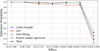 |
Fig. 14 Detection probability as a function of the S/NPSD intervals. In the interval notation used, a round bracket ‘)’ indicates an open interval, excluding the ending point, while a square bracket ‘[’ indicates a closed interval, including the starting point. |
6.2 Detection probability and TESS magnitude
The S/NPSD value of observed TESS light curves is expected to decrease for fainter systems, that is systems with higher TESS magnitude. We have verified this on the sample of polars. The result is shown in Fig. 15. By comparing this with the S/NPSD threshold determined in Sect. 6.1 we can determine a limiting TESS magnitude for orbital period detection in the sample.
The measurement of S/NPSD in the observed light curves was performed using the same methodology applied for the simulated light curves (see Appendix E) but with some additional considerations. The TESS light curve of TIC 840418301 (sector 48) which we used to produce simulated light curves presented only one periodic signal, which was ascribed to the orbital period. In our sample of polars, the situation is not that simple and other periodic signals – including 1/2 Porb as discussed above – may be present in the PSD. Such additional signals must be removed. To this end we implemented the following criteria:
If the frequency peak at 1/2 Porb is present in the PSD, only the stronger of the 1/2 Porb and the Porb frequency peak is associated with the signal, since this would be the signal that would be predominantly detected. In the noise-only signal construction, both frequency peaks are removed from the PSD.
In the estimation of the noise power, not only the frequency peak associated with the signal is removed from the PSD, but also additional short periodic signals (P ~ 0–500 min) that may have their origin in additional astrophysical processes, for example the spin period in asynchronous systems, or arise from phenomena like beat frequencies or aliasing. The identification of such periodic signals was performed through visual inspection of each individual light curve. In practice, aliased frequency peaks are straightforward to identify as they appear as a series of harmonics, narrow and regularly spaced in the low-period region of the PSD. Additional signals, such as the beat frequencies normally appear as high-power and narrow peaks. These peaks would lead to an overestimation of the noise if not removed. Frequency peaks that were ambiguous and could plausibly originate from noise were retained.
Figure 15 presents the measured S/NPSD values from the observed TESS light curves against the TESS magnitudes of the corresponding objects. We note that the estimation of S/NPSD requires the presence of a periodic signal in the PSD. In some cases, a periodic signal appears in the Lomb-Scargle periodogram but is absent from the PSD calculated as described in Appendix E. This typically occurs in noisy light curves, suggesting that the frequency peak in the Lomb-Scargle periodogram may have arisen purely from noise. Applying the methodology of Appendix E, a periodic signal is present in the PSD of 223 out of 235 TESS light curves, hence we have 223 S/NPSD values. The remaining cases do not appear in Fig. 15.
Figure 15 confirms the expected trend: as the TESS magnitude increases, S/NPSD tends to decrease. This reflects the fact that the noise level in the TESS light curves increases for fainter objects. However, the S/N also depends on the amplitude of the astrophysical signal. Individual polars exhibit different amplitudes in their periodicities due to factors such as the inclination of the system, which can affect the visibility of the hotspot. Therefore, the S/NPSD values present a significant dispersion for a given TESS magnitude. This means that (S/NPSD)min does not translate to a definite value for the limiting TESS magnitude for a detectable period, but only an approximate range, where prudence should rule the interpretation of eventual period detections. Specifically, from the 223 observed light curves in which S/NPSD could be estimated, approximately 9% of the light curves with TESS magnitudes T ≳ 17 mag have a S/NPSD below the threshold of (S/NPSD)min = 0.004, suggesting a false positive rate of around 9% for systems fainter than T ≳ 17 mag. For such faint systems, the actual S/NPSD associated with a period measurement should be calculated following Appendix E to assess the reliability of the measurement. For TESS magnitudes T ≳ 19 mag, not covered by the sample of observations of this work, the same trend observed in Fig. 15 is expected to apply and the percentage of light curves with S/NPSD below the detection reliability threshold likely increases.
7 Summary and conclusions
We determined orbital periods for 93 out of 95 polars with TESS two-minute cadence light curves from Sectors 1-63. For 85 systems our measured values are consistent with values previously reported in the literature. The remaining ten objects comprise four asynchronous CVs with complex power-spectra and four systems where the TESS-based periods differ from those reported in the literature. For only 2 of the 95 systems no period could be found because of high noise levels in their TESS light curves.
For the four asynchronous systems our detailed analysis yielded an identification of both the orbital period, Porb, and the spin period of the primary, Pspin (see Table 1). We detected new side-band periods for BY Cam and IGR J19552+0044, and revised the multiple periods present in the TESS light curves of CD Ind, confirming the physical origin of many of the low-power side-band periods presented in the previous literature (see Appendix B).
A detailed examination of the four polars where our period determination is discrepant from the previous literature values yielded revised or improved values. Some of these measurements, however, remain tentative due to a low S/N and follow-up observations are recommended.
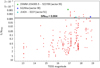 |
Fig. 15 S/NPSD of observed TESS light curves as a function of the TESS magnitude. The black horizontal line indicates the limiting S/NPSD for a reliable orbital period detection, S/NPSD = 0.004, determined with simulations (see Sect. 6.1). In Sect. 4.6.2, periods were provided for 2XMM J154305.5-52270, GQ Mus, and J1424-0227 (marked here with different plotting symbols and colours), but our new periods as well as previous values presented for them in the literature remain questionable, consistent with the location of these systems beyond the S/NPSD threshold. |
7.1 Reliability of TESS-based CV period detections
Earlier studies have highlighted the potential of TESS to refine or improve period detections of CVs (see Bruch 2024b). The overall good agreement between our measured orbital periods and the literature values for the majority of the polars confirms the suitability and efficiency of TESS light curves for the measurement of orbital periods in such systems. Moreover, it underscores the robustness of our analysis methodology.
Specifically, by simulating periodic light curves with varying noise levels and testing whether the orbital period can be recovered, we established a probabilistic framework for the detection success across different S/NPSD intervals, where the S/NPSD of a light curve is a measure of the significance of the frequency peak associated with the orbital period with respect to the noise. A threshold value of (S/NPSD)min = 0.004 was determined at which the detection probability of orbital periods in TESS light curves of polars sharply decreases from a nearly 100% recovery rate to below the 50% level (see Fig. 14). The comparison of the measured S/NPSD in an observed TESS light curve with this threshold enables us to estimate the reliability of a period detection.
We note that the above S/NPSD threshold value was derived from simulations based on a specific observed TESS light curve – TIC 840418301 (sector 48) with an orbital period of Porb = 82.4 min - and could be subject to some variation for systems with longer periods and when red noise significantly contributes to the power-law shape of the PSD. However, in CVs, the orbital periods fall within a confined region of high frequencies in the PSD of TESS light curves. Since red noise affects lower-frequency power, its consideration would only lead to a more optimistic S/NPSD threshold, i.e. a lower limiting S/NPSD value (see Eq. (E.2)), and it would not obscure the frequency peak associated with the orbital period (see Fig. E.1).
The S/NPSD was measured in all observed TESS light curves of our sample. We found that for systems with TESS magnitudes T ≳ Tlim ≈ 17 mag, a significant fraction of light curves were found to be too noisy to accurately detect the orbital period. We note that the value for Tlim is not a precise limit because polars are variable, and they can exhibit both high and low states during an observation. Transitions between these states occur on timescales of days to years, with brightness changes of a few magnitudes (see Kalomeni 2012). In addition, Duffy et al. (2022) found that short-duration accretion states are relatively common among polars. These states can last from a few days to ~50 days. Based on the trend observed in Fig. 15, we suggest the following practical guideline for detection reliability based on TESS magnitude:
Reliable: T < 17 mag;
Uncertain: 17 < T < 19 mag;
Likely unreliable: T > 19 mag.
In the future we intend to complement this study with samples covering fainter TESS magnitudes in order to find the approximate limiting brightness that completely impedes the detection of orbital periods in CVs. Our methodology will also be useful for the confirmation of CV candidates and, more generally, in the search for periods with TESS for other types of objects.
7.2 Noise level in TESS light curves
We have expanded on our earlier studies of the dependence of the noise level in TESS light curves on the brightness of the stars. Specifically, we have determined the correlation between the TESS magnitude and the noise level in flattened TESS light curves, that had been cleaned from the known astrophysical signals (see Fig. 13). Compared to the samples of M dwarfs for which the same relation was studied by us (Stelzer et al. 2016; Raetz et al. 2020), the polars have much fainter T magnitudes. To bridge the gap to the polars, we complement the bright and nearby M dwarfs from our earlier works with a fainter M dwarf sample. Across the M dwarfs we observe a well defined lower envelope and a sparse population of stars with higher noise levels that – according to our earlier studies – is likely associated with intrinsic stellar variability hidden in the noise. The polars extend this trend of increasing noise with T magnitude to fainter stars, albeit with a larger scatter. We suspect that the scatter of the noise in polars for given T magnitude derives from flickering and from the fact that T magnitude may not represent the actual brightness of the polar at the time of observation, as discussed in Sect. 7.1. A dedicated study would be useful to constrain the origin of the noise level in TESS light curves of polars.
We provide a functional form for the lower envelope of the noise in TESS light curves, expressed through the parameter S flat. This relation allows the expected intrinsic noise in TESS light curves to be estimated based on the object’s brightness. High noise levels can have a significant impact on the detection of low-amplitude astrophysical modulations in TESS light curves, and by characterising this noise we provide a useful reference for future variability studies in TESS light curves.
 |
Fig. 16 Gaia colour-magnitude diagram showing the sample of polars with TESS two-minute cadence light curves on a background of Gaia DR3 sources with distances from Bailer-Jones et al. (2021) and a parallax error of <1% of the parallax value. The colour-coding corresponds to the measured orbital periods. |
7.3 TESS-polars in the Gaia colour-magnitude diagram
Figure 16 displays the TESS sample of polars studied in this work in the Gaia colour-magnitude diagram (CMD). As can be seen from the comparison with Gaia DR3 sources from Bailer-Jones et al. (2021), polars are located between the main sequence and the white dwarf sequence. All the systems in our sample have a Gaia counterpart, and the absolute magnitude in the Gaia G band was calculated making use of the Bailer-Jones et al. (2021) distances. The colour-coding in Fig. 16 marks the measured orbital periods and shows that systems with longer periods are located closer to the main sequence, while systems with shorter periods approach the WD sequence. The long-term evolution of CVs is characterised by the transition from longer to shorter orbital periods due to the loss of angular momentum (see e.g. Knigge 2011 and Kalomeni et al. 2016). In less evolved systems, the donor star is still massive and bright such that its contribution dominates the luminosity of the system. As the systems evolve, the donor mass decreases as a consequence of the mass transfer to the WD and its contribution to the luminosity of the system becomes less significant. The observed period distribution is therefore in agreement with the expected evolution of CVs from the lower envelope of the main sequence to the WD sequence. This result is consistent with earlier findings reported by Abril et al. (2019) from the CV catalogues from Downes et al. (2001) and Ritter & Kolb (2003). We note in Fig. 16 an apparent cavity around MG ~ 10 and GBP − GRP ~ 0.5. This feature arises due to the tracks that CVs follow in the Hertzsprung-Russell diagram as their mass accretion rate varies (see Dubus & Babusiaux 2024). A measurement of donor masses will ultimately confirm this evolutionary sequence of CVs in the HR diagram.
Data availability
The table described by Table A.1 is available at the CDS via https://cdsarc.cds.unistra.fr/viz-bin/cat/J/A+A/703/A166
Acknowledgements
We wish to thank the anonymous referee for constructive comments and suggestions that helped improve the clarity and quality of this article. We are also grateful to Alex Binks and Simone Scaringi for helpful discussions and valuable comments on this work. Santiago Hernández-Díaz acknowledges financial support from Deutsche Forschungsgemeinschaft (DFG) under grant number STE 1068/6-2. This work is based on data collected by the TESS mission and obtained from the MAST data archive at the Space Telescope Science Institute (STScI). Funding for the missions is provided by the NASA Explorer Program and the NASA Science Mission Directorate. STScI is operated by the Association of Universities for Research in Astronomy, Inc., under NASA contract NAS 5-26555. This work has made use of data from the European Space Agency (ESA) mission Gaia (https://www.cosmos.esa.int/gaia), processed by the Gaia Data Processing and Analysis Consortium (DPAC, https://www.cosmos.esa.int/web/gaia/dpac/consortium). Funding for the DPAC has been provided by national institutions, in particular the institutions participating in the Gaia Multilateral Agreement.
Appendix A Sample properties and results from period search for the catalogue of polars
Table A.1 provides a summary of the structure of the main data table resulting from our work. It comprises basic coordinates, identifiers, photometry from TESS and Gaia, and the results obtained from the period search on their TESS light curves.
Description of the 24 columns in the sample of polars, including identifiers, coordinates, photometric data, orbital period measurements, and references.
Appendix B Periodicities detected in asynchronous systems
Identified periods in the TESS light curves of TIC 339374052 (alias BY Cam) (sectors 19 and 59).
Identified periods in the TESS light curve of TIC 228975750 (alias IGR J19552+0044) (sector 54).
Identified periods in the TESS light curves of TIC 231666244 (alias CD Ind) (sectors 1 and 27).
Identified periods in the TESS light curve of TIC 369210348 (alias Paloma) (sector 19).
Appendix C Simulation of TESS light curves
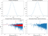 |
Fig. C.1 PDF and PSD of the original observed TESS light curve of TIC 840418301 (sector48) and a simulated light curve for comparison. The normal distribution characterising the PDF is conserved and the simulated PSD correctly replicates the PSD of the observed light curve. |
The algorithm from Timmer and König (Timmer & König 1995) (hereafter denoted as TK95 algorithm), has been implemented to simulate TESS light curves. This method generates synthetic light curves from an underlying PSD model. In this study, the PSD model corresponds to a smoothed version of the observed PSD from TIC 840418301 (sector48).
To compute the PSD of the observed light curve of TIC 840418301 (sector 48), a Kaiser window with β = 5 is used. This value for the parameter β is higher than the value used in the generation of the Fourier power spectrum for the detection of the orbital periods, where β = 3 was used. In the detection of orbital periods, maintaining a high-frequency resolution was primary. On the contrary, in the simulation of light curves, a greater compromise with the spectral leakage reduction is preferred, effectively diminishing the distortion in the PSD estimation. However, a precise reproduction of the orbital period signal in the simulated light curves is required, and therefore a low value for ßis still convenient.
To estimate the underlying PSD of the observed light curve of TIC 840418301 (sector48), the LOWESS (Locally Weighted Scatterplot Smoothing) non-parametric regression method (Cleveland 1979, Cleveland & Devlin 1988) is additionally implemented. The LOWESS method reveals the underlying form of the PSD, smoothing the high-frequency noise, which is enhanced during the simulation process, and capturing the local variations represented by the frequency peaks. To this extent, the non-parametric nature of the method solves the problem of specifying a global analytical function to fit a model to the PSD of the observed light curve. This estimated PSD will be the target PSD which should be matched by the TK95 algorithm in the production of simulated light curves.
The TK95 algorithm generates a stochastic realisation of a PSD model. In our case, this means that the height of the frequency peak can differ across different simulations. To ensure consistency between the frequency peak height in the observed PSD of TIC 840418301 (sector 48) and that of simulated light curves, only simulations where the peak height deviated by no more than 5% from the observed value were considered.
The TK95 algorithm is designed to preserve only the initial two statistical moments of the original data set, the mean value and the variance. Higher-order statistical moments, such as skewness and kurtosis, are disregarded in the resulting simulated data. Thus, the TK95 algorithm is only suitable for generating simulated data sets that exhibit a Gaussian distribution. To produce simulations that match the observed light curve’s statistical characteristics, the observed light curve’s PDF must also be normally distributed. For the observed light curve of TIC 840418301 (sector 48), normality diagnostics confirm the light curve’s normal distribution, making it suitable as a template for simulation-recovery tests (details in Appendix D).
Another algorithm, based on TK95, can match both the PSD and PDF of observed light curves (Emmanoulopoulos et al. 2013). While advantageous for the simulation of observed light curves that present deviations from normality, it struggles to reproduce the frequency peaks in the PSD of CVs light curves, leading to its exclusion from this analysis.
Finally, this analysis involves generating simulated light curves with varying levels of white noise. The white noise, wn ~ ***(eq11)*** , is added to the simulated light curves, with its level regulated by the variance ***(eq12)***
 .
.
Appendix D Normality diagnostics
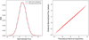 |
Fig. D.1 Normality plots for the light curve of TIC 840418301 in sector48. Left: Light curve histogram with the theoretical normal probability density function overplotted. The histogram’s values correspond with the probability density function at the bin. The histogram is normalised such thattheintegralovertheentirerangeis1.Right: Ordered sample data against the theoretical quantiles of the normal distribution. |
The normality of the observed light curve of TIC 840418301 (sector 48) was evaluated using both graphical and statistical methods.
As a first step, the light curve was flattened to subtract the periodic modulation, effectively isolating the noise. This ensures that the normality evaluation focuses solely on the stochastic noise, rather than the deterministic periodicity present in the original data.
In Fig. D.1, two graphical representations are presented: the light curve’s histogram (left panel) and a normal probability plot (right panel). The histogram closely matches the theoretical normal PDF defined by the light curve’s mean and standard deviation. The normal probability plot reveals minor deviations from linearity at the extremes, indicating certain level of truncation in the data, that is, there are not observations covering the full range given by the normal distribution. Aside from this, no important deviations from normality are observed.
The skewness and kurtosis were estimated as ***(eq13)*** and b2 = 3.043 ± 0.039, respectively. The obtained skewness is, within the standard error, in complete agreement with a normal distribution, while the obtained kurtosis value is sufficiently close to 3 and deviations from normality can be considered as negligible.
The Shapiro-Wilk normality test (Shapiro & Wilk 1965) was performed yielding a p-value = 0.67. The Shapiro-Wilk test presents one important defect to be taken into account: it does not perform well with large data sets. Hence, additional normality diagnostics are considered.
The D’Agostino’s K2 test (D’Agostino & Pearson 1973) and the Anderson-Darling test (Anderson & Darling 1952) were implemented producing a p-value = 0.52 and a A2 statistic of A2 = 0.355, respectively. For a significance level of 0.05, the associated critical value in the Anderson-Darling test is 0.787.
At a typical significance level of 0.05, none of the normality tests rejects the null hypothesis that the light curve is drawn from a normal distribution.
In this work, the Python implementations of the aforementioned normality tests included in the package Scipy were used.
Appendix E Signal-to-noise ratio measurement
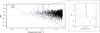 |
Fig. E.1 Measurement of S/NPSD in a simulated light curve. The frequency peak in the PSD of the light curve corresponding to the orbital period is identified as the signal. After the removal of the frequency peak, the remaining signal is associated with the noise. |
The measurement of the signal-to-noise ratio in the PSD, S/NPSD, of simulated light curves is conducted with a methodology based on Fourier transforms. As explained in Sect. 6.1, the light curve of TIC 840418301 (sector48) serves as a template for our simulations.
For each simulated light curve, we first computed the PSD with the use of a Kaiser window (Kaiser & Schafer 1980) with β = 12. The choice of a high value for the parameter β responds to the priority of reducing the spectral leakage in the PSD, which would otherwise affect the signal’s power estimation. For the template light curve of TIC 840418301 (sector48), the precise location of the frequency peak associated with the orbital period is already known from the period search described in Sect. 4 and a loss in the frequency resolution does not act to the detriment of the S/NPSD measurement. The measured orbital period in TIC 840418301 (sector 48) is Porb = 82.4 min. The frequency peak in the PSD that corresponds to the orbital period is therefore readily identified. This peak represents the signal of interest and its associated power is computed by integrating the area under the frequency peak in the PSD,
 (E.1)
(E.1)
where ƒlower and ƒupper denote the lower and upper frequencies that determine the range that captures the frequency peak in its entirety.
Next, the frequency peak corresponding with the orbital period is removed from the PSD. For the removal of the frequency peak, consecutive data points with continuously decreasing values on both sides of the peak’s maximum are considered, that is, data points PS D(ƒi−1) holding PS D(ƒi−1) < PS D(ƒi) are selected on the left of the peak’s maximum and data points PS D(ƒi+1) holding PS D(ƒi+1) < PS D(ƒi) are selected on the right of the peak’s maximum, where ƒi denotes the discrete Fourier frequencies. All other parts of the PSD are then associated with the noise (see Fig. E.1) and its power is computed, as before, by integration,
 (E.2)
(E.2)
where ƒmin and ƒmax denote the minimum and maximum frequencies in the PSD.
The S/NPSD is thus
 (E.3)
(E.3)
We note that, in the measurement of the S/NPSD, the DC component, given by the zero Fourier frequency component, has not been included, as the relevant information here considered is the predominance of the frequency peak associated with the orbital period with respect to the noise that, potentially, could hinder its detection.
References
- Abril, J., Schmidtobreick, L., Ederoclite, A., & López-Sanjuan, C. 2019, MNRAS, 492, L40 [Google Scholar]
- Anderson, T. W., & Darling, D. A. 1952, Ann. Math. Stat., 23, 193 [Google Scholar]
- Applegate, J. H. 1992, ApJ, 385, 621 [Google Scholar]
- Applegate, J. H., & Patterson, J. 1987, ApJ, 322, L99 [NASA ADS] [CrossRef] [Google Scholar]
- Bailer-Jones, C. A. L., Rybizki, J., Fouesneau, M., Demleitner, M., & Andrae, R. 2021, VizieR Online Data Catalog: Distances to 1.47 billion stars in Gaia EDR3 (Bailer-Jones+, 2021), VizieR On-line Data Catalog: I/352 [Google Scholar]
- Binks, A. S., Jeffries, R. D., Sacco, G. G., et al. 2022, MNRAS, 513, 5727 [NASA ADS] [Google Scholar]
- Biser, I., & Millman, G. 1965, Tables of Offset Circle Probabilities for a Normal Bivariate Elliptical Distribution, Technical report ECQM-2625 (U.S. Army Electronics Command) [Google Scholar]
- Bochkarev, N. G., Karitskaia, E. A., & Shakura, N. I. 1979, Soviet Ast., 23, 8 [Google Scholar]
- Bruch, A. 2021, MNRAS, 503, 953 [NASA ADS] [CrossRef] [Google Scholar]
- Bruch, A. 2022, MNRAS, 514, 4718 [NASA ADS] [CrossRef] [Google Scholar]
- Bruch, A. 2023a, MNRAS, 519, 352 [Google Scholar]
- Bruch, A. 2023b, MNRAS, 525, 1953 [CrossRef] [Google Scholar]
- Bruch, A. 2024a, ApJS, 273, 6 [NASA ADS] [CrossRef] [Google Scholar]
- Bruch, A. 2024b, AJ, 168, 121 [Google Scholar]
- Campbell, C. G. 1985, MNRAS, 215, 509 [Google Scholar]
- Campbell, C. G. 1986, MNRAS, 219, 589 [Google Scholar]
- Campbell, C. G., & Schwope, A. D. 1999, A&A, 343, 132 [NASA ADS] [Google Scholar]
- Christiansen, J. L., Jenkins, J. M., Caldwell, D. A., et al. 2012, PASP, 124, 1279 [NASA ADS] [CrossRef] [Google Scholar]
- Cleveland, W. S. 1979, J. Am. Stat. Assoc., 74, 829 [Google Scholar]
- Cleveland, W. S., & Devlin, S. J. 1988, J. Am. Stat. Assoc., 83, 596 [CrossRef] [Google Scholar]
- Cooley, J. W., & Tukey, J. W. 1965, Math. Comp., 19, 297 [CrossRef] [MathSciNet] [Google Scholar]
- Cropper, M. 1990, Space Sci. Rev., 54, 195 [CrossRef] [Google Scholar]
- D’Agostino, R., & Pearson, E. S. 1973, Biometrika, 60, 613 [Google Scholar]
- Denisenko, D. V., Drake, A. J., Djorgovski, S. G., et al. 2011, Astron. Lett., 37, 858 [Google Scholar]
- Diaz, M. P., & Steiner, J. E. 1989, ApJ, 339, L41 [Google Scholar]
- Downes, R. A., Webbink, R. F., Shara, M. M., et al. 2001, PASP, 113, 764 [Google Scholar]
- Dubus, G., & Babusiaux, C. 2024, A&A, 683, A247 [NASA ADS] [CrossRef] [EDP Sciences] [Google Scholar]
- Duffy, C., Ramsay, G., Wu, K., et al. 2022, MNRAS, 516, 3144 [Google Scholar]
- Emmanoulopoulos, D., McHardy, I. M., & Papadakis, I. E. 2013, MNRAS, 433, 907 [NASA ADS] [CrossRef] [Google Scholar]
- European Space Agency 2024, Gaia Archive, https://gea.esac.esa.int/archive/ Accessed: 2023-12-10 [Google Scholar]
- Ferrario, L., Wickramasinghe, D. T., & Tuohy, I. R. 1989, ApJ, 341, 327 [NASA ADS] [CrossRef] [Google Scholar]
- Gabdeev, M. M. 2015, Astrophys. Bull., 70, 460 [Google Scholar]
- Gaia Collaboration (Vallenari, A., et al.) 2023, A&A, 674, A1 [NASA ADS] [CrossRef] [EDP Sciences] [Google Scholar]
- Harrison, T. E., & Campbell, R. K. 2015, ApJS, 219, 32 [Google Scholar]
- Honeycutt, R. K., & Kafka, S. 2005, MNRAS, 364, 917 [NASA ADS] [CrossRef] [Google Scholar]
- Hyndman, R. J. 2011, Moving Averages, ed. M. Lovric (Berlin, Heidelberg: Springer Berlin Heidelberg), 866 [Google Scholar]
- Ilkiewicz, K., Scaringi, S., Littlefield, C., & Mason, P. A. 2022, MNRAS, 516, 5209 [Google Scholar]
- Jenkins, J. M., Chandrasekaran, H., McCauliff, S. D., et al. 2010, SPIE Conf. Ser., 7740, 77400D [Google Scholar]
- Joseph, W. M., Stelzer, B., Magaudda, E., & Vicánek Martinez, T. 2024, A&A, 688, A49 [NASA ADS] [CrossRef] [EDP Sciences] [Google Scholar]
- Kaiser, J., & Schafer, R. 1980, IEEE Trans. Acoust. Speech Signal Process., 28, 105 [Google Scholar]
- Kalomeni, B. 2012, MNRAS, 422, 1601 [Google Scholar]
- Kalomeni, B., Nelson, L., Rappaport, S., et al. 2016, ApJ, 833, 83 [NASA ADS] [CrossRef] [Google Scholar]
- Knigge, C. 2011, ASP Conf. Ser., 447, 3 [Google Scholar]
- Lamb, F. K., Aly, J. J., Cook, M. C., & Lamb, D. Q. 1983, ApJ, 274, L71 [Google Scholar]
- Levenberg, K. 1944, Quarter. Appl. Math., 2, 164 [Google Scholar]
- Littlefield, C., Garnavich, P., Mukai, K., et al. 2019, ApJ, 881, 141 [NASA ADS] [CrossRef] [Google Scholar]
- Littlefield, C., Hoard, D. W., Garnavich, P., et al. 2023, AJ, 165, 43 [Google Scholar]
- Lomb, N. R. 1976, Ap&SS, 39, 447 [Google Scholar]
- Marsh, T. R., Morales-Rueda, L., Steeghs, D., et al. 2002, ASP Conf. Ser., 261, 200 [Google Scholar]
- Mason, P. A., Liebert, J., & Schmidt, G. D. 1989, ApJ, 346, 941 [Google Scholar]
- Mason, P. A., Fisher, P. L., & Chanmugam, G. 1996, A&A, 310, 132 [Google Scholar]
- Mason, P. A., Ramsay, G., Andronov, I., et al. 1998, MNRAS, 295, 511 [Google Scholar]
- Mason, P. A., Littlefield, C., Monroy, L. C., et al. 2022, ApJ, 938, 142 [Google Scholar]
- Mennickent, R. E., Pietrzynski, G., Diaz, M., & Gieren, W. 2003, A&A, 399, L47 [NASA ADS] [CrossRef] [EDP Sciences] [Google Scholar]
- Myers, G., Patterson, J., de Miguel, E., et al. 2017, PASP, 129, 044204 [Google Scholar]
- Nagel, E., Czesla, S., & Schmitt, J. H. M. M. 2016, A&A, 590, A47 [NASA ADS] [CrossRef] [EDP Sciences] [Google Scholar]
- Ok, S., & Schwope, A. 2022, A&A, 662, A116 [NASA ADS] [CrossRef] [EDP Sciences] [Google Scholar]
- Paegert, M., Stassun, K. G., Collins, K. A., et al. 2022, VizieR Online Data Catalog: TESS Input Catalog version 8.2 (TIC v8.2) (Paegert+, 2021), VizieR On-line Data Catalog: IV/39 [Google Scholar]
- Patterson, J. 1994, PASP, 106, 209 [Google Scholar]
- Pavlenko, E., Andreev, M., Babina, Y., & Malanushenko, V. 2013, ASP Conf. Ser., 469, 343 [Google Scholar]
- Raetz, S., Stelzer, B., & Scholz, A. 2020, Astron. Nachr., 341, 519 [NASA ADS] [CrossRef] [Google Scholar]
- Ricker, G. R., Winn, J. N., Vanderspek, R., et al. 2015, J. Astron. Teles. Instrum. Syst., 1, 014003 [Google Scholar]
- Ritter, H., & Kolb, U. 2003, A&A, 404, 301 [NASA ADS] [CrossRef] [EDP Sciences] [Google Scholar]
- Scargle, J. D. 1982, ApJ, 263, 835 [Google Scholar]
- Scaringi, S. 2014, MNRAS, 438, 1233 [Google Scholar]
- Schwarz, R., Schwope, A. D., Staude, A., & Remillard, R. A. 2005, A&A, 444, 213 [NASA ADS] [CrossRef] [EDP Sciences] [Google Scholar]
- Schwarz, R., Schwope, A. D., Staude, A., et al. 2007, A&A, 473, 511 [NASA ADS] [CrossRef] [EDP Sciences] [Google Scholar]
- Schwope, A. D. 1990, Rev. Mod. Astron., 3, 44 [Google Scholar]
- Schwope, A. D. 2025, A&A, 698, A106 [NASA ADS] [CrossRef] [EDP Sciences] [Google Scholar]
- Schwope, A. D., & Mengel, S. 1997, Astron. Nachr., 318, 25 [Google Scholar]
- Servillat, M., Grindlay, J., van den Berg, M., et al. 2012, ApJ, 748, 32 [Google Scholar]
- Shapiro, S. S., & Wilk, M. B. 1965, Biometrika, 52, 591 [Google Scholar]
- Silber, A. D., Szkody, P., Hoard, D. W., et al. 1997, MNRAS, 290, 25 [Google Scholar]
- Sobolev, A. V., Zhilkin, A. G., Bisikalo, D. V., & Buckley, D. A. H. 2021, Astron. Rep., 65, 392 [Google Scholar]
- Space Telescope Science Institute 2024, MAST Portal, https://mast.stsci.edu/portal/Mashup/Clients/Mast/Portal.html Accessed: 2023-0920 [Google Scholar]
- Sparks, W. M., & Sion, E. M. 2021, ApJ, 914, 5 [NASA ADS] [CrossRef] [Google Scholar]
- Stassun, K. G., Oelkers, R. J., Paegert, M., et al. 2019, AJ, 158, 138 [Google Scholar]
- Stelzer, B., Damasso, M., Scholz, A., & Matt, S. P. 2016, MNRAS, 463, 1844 [NASA ADS] [CrossRef] [Google Scholar]
- Stelzer, B., de Martino, D., Casewell, S. L., Wynn, G. A., & Roy, M. 2017, A&A, 598, L6 [EDP Sciences] [Google Scholar]
- Stelzer, B., Bogner, M., Magaudda, E., & Raetz, S. 2022, A&A, 665, A30 [NASA ADS] [CrossRef] [EDP Sciences] [Google Scholar]
- Stockman, H. S., Schmidt, G. D., & Lamb, D. Q. 1988, ApJ, 332, 282 [Google Scholar]
- Taylor, M. B. 2005, ASP Conf. Ser., 347, 29 [Google Scholar]
- Timmer, J., & König, M. 1995, A&A, 300, 707 [Google Scholar]
- Tovmassian, G., González-Buitrago, D., Thorstensen, J., et al. 2017, A&A, 608, A36 [NASA ADS] [CrossRef] [EDP Sciences] [Google Scholar]
- van den Berg, M., Penner, K., Hong, J., et al. 2012, ApJ, 748, 31 [Google Scholar]
- VanderPlas, J. T. 2018, ApJS, 236, 16 [Google Scholar]
- Vladimirov, V., Shurpakov, S., Denisenko, D., et al. 2014, ATel, 5726, 1 [Google Scholar]
- Vogel, J., Schwope, A. D., & Gänsicke, B. T. 2007, A&A, 464, 647 [NASA ADS] [CrossRef] [EDP Sciences] [Google Scholar]
- Wang, Q., Qian, S., Han, Z., et al. 2020, ApJ, 892, 38 [Google Scholar]
- Wang, Q., Qian, S., & Liao, W. 2021, PASP, 133, 114201 [Google Scholar]
- Warner, B. 1995, Cataclysmic Variable Stars (Cambridge: Cambridge University Press), 28 [Google Scholar]
- Wilson, R. E. 2006, ASP Conf. Ser., 349, 71 [Google Scholar]
- Wynn, G. A., & King, A. R. 1992, MNRAS, 255, 83 [NASA ADS] [CrossRef] [Google Scholar]
All Tables
Orbital and spin periods of asynchronous systems in the sample of polars observed with TESS in two-minute cadence.
Description of the 24 columns in the sample of polars, including identifiers, coordinates, photometric data, orbital period measurements, and references.
Identified periods in the TESS light curves of TIC 339374052 (alias BY Cam) (sectors 19 and 59).
Identified periods in the TESS light curve of TIC 228975750 (alias IGR J19552+0044) (sector 54).
Identified periods in the TESS light curves of TIC 231666244 (alias CD Ind) (sectors 1 and 27).
Identified periods in the TESS light curve of TIC 369210348 (alias Paloma) (sector 19).
All Figures
|
Fig. 1 Properties of the sample of polars with two-minute time-resolution TESS light curves. Left panel: histogram of TESS magnitudes. Right panel: histogram of distances (from Bailer-Jones et al. 2021). |
| In the text | |
|
Fig. 2 Illustration of the results from different period detection methods for a case where the dominant period is 1 /2 Porb (from left to right): Lomb-Scargle periodogram, ACF, and Fourier power spectrum. The example refers to TIC 124404442 (alias V1043 Cen) (sector 37). The red vertical lines indicate the signals at 1/2 Porb, while the green vertical lines indicate the true orbital period (Sparks & Sion 2021). In this light curve, all three methods failed to identify the orbital period. We note that although the autocorrelation coefficient at the true orbital period is higher than that at 1/2 Porb in the ACF plot, the subsequent FFT applied to the autocorrelation coefficients yields a stronger signal in 1/2 Porb. |
| In the text | |
|
Fig. 3 Phase plots for the light curve of TIC 258799357 (alias EP Dra) (sector 26), an eclipsing polar, as an example of a light curve where the dominating modulation is at 1/2 Porb. Left panel: light curve folded over the detection at 1/2 Porb. Right panel: light curve folded over the true orbital period (Schwope & Mengel 1997). The true orbital period (right panel) displays the pattern corresponding to one complete orbit of the primary star around the secondary, with the eclipse distinctly visible around phase 0.5. |
| In the text | |
|
Fig. 4 Zoomed-in view of the Lomb-Scargle periodograms of the TESS light curves of TIC 339374052 (alias BY Cam). Top panels: Sector 19. Bottom panels: Sector 59. The red lines mark the positions of the different periodicities that were measured (see Table B.1). |
| In the text | |
|
Fig. 5 Zoomed-in view of the Lomb-Scargle periodogram of the TESS light curve of TIC 228975750 (alias IGR J19552+0044) (sector 54). The red lines mark the positions of the different periods that were measured (see Table B.2). |
| In the text | |
|
Fig. 6 Zoomed-in view of the Lomb-Scargle periodograms of the TESS light curves of TIC 231666244 (alias CD Ind). Top panels: Sector 1. Bottom panels: Sector 27. The red lines mark the positions of the different periods that were measured (see Table B.3). |
| In the text | |
|
Fig. 7 Zoomed-in view of the Lomb-Scargle periodogram of the TESS light curve of TIC 369210348 (alias Paloma) (sector 19). The red lines mark the positions of the different periods that were measured (see Table B.4). |
| In the text | |
|
Fig. 8 Top panel: Lomb-Scargle periodogram of the two-minute cadence TESS light curve of TIC 1140118632 (alias 2XMM J154305.5-522709) (sector 39). Centre panel: zoomed-in view of the frequency peak located at 144.6 min. Bottom panel: zoomed-in view of the frequency peak located at 260.90 ± 0.29 min. The red lines mark the positions of the frequency peaks. |
| In the text | |
|
Fig. 9 Left panels: Lomb-Scargle periodograms of the TESS light curves of TIC 908535248 (alias GQ Mus) from Sector 37 (top) and Sector 38 (bottom). Right panels: zoomed-in view of the region around the highest frequency peaks, located at 249.64 ± 0.57 min (top for Sector 37) and at 495.1 ± 2.3 min (bottom for Sector 38). The red lines mark the positions of the frequency peaks. |
| In the text | |
|
Fig. 10 Zoomed-in views of the frequency peak at ~ 200.8 min in the Lomb-Scargle periodograms of the TESS light curves of TIC 94840820 (alias J0733+2619). Top panel: Sector 44. Centre panel: Sector 45. Bottom panel: Sector 46. The red lines mark the positions of the frequency peaks. |
| In the text | |
|
Fig. 11 Top panel: Lomb-Scargle periodogram of the TESS light curve of TIC 1002329407 (alias J1424-0227) (sector 51). Bottom panel: zoomed-in view of the frequency peak located at 121 .636 ± 0.063 min. The red lines mark the positions of the frequency peaks. |
| In the text | |
|
Fig. 12 Top panel: Lomb-Scargle periodogram for TIC 641322558 (sector 58). Bottom panel: Lomb-Scargle periodogram for TIC 953321496 (sector 46). The low S/N impedes the identification of periodic signals. The red lines mark the positions of the orbital periods reported in the literature (see Vladimirov et al. 2014 and Stelzer et al. 2017). |
| In the text | |
|
Fig. 13 Relation between Sflat and TESS magnitude for polars (pink) compared to the same relation for the M dwarf sample from Stelzer et al. (2022) (red) and a subsample of M dwarfs from Joseph et al. (2024) (blue). The TESS light curves of the latter were analysed by us (see Sect. 5). The lower envelope of the Sflat distribution (green dashed line) was obtained by fitting a second-order polynomial to the lower 25% quantile of the data. The two-hour rmsCDPP values for all objects in the three samples are presented for comparison (see Sect. 5 for details). |
| In the text | |
|
Fig. 14 Detection probability as a function of the S/NPSD intervals. In the interval notation used, a round bracket ‘)’ indicates an open interval, excluding the ending point, while a square bracket ‘[’ indicates a closed interval, including the starting point. |
| In the text | |
|
Fig. 15 S/NPSD of observed TESS light curves as a function of the TESS magnitude. The black horizontal line indicates the limiting S/NPSD for a reliable orbital period detection, S/NPSD = 0.004, determined with simulations (see Sect. 6.1). In Sect. 4.6.2, periods were provided for 2XMM J154305.5-52270, GQ Mus, and J1424-0227 (marked here with different plotting symbols and colours), but our new periods as well as previous values presented for them in the literature remain questionable, consistent with the location of these systems beyond the S/NPSD threshold. |
| In the text | |
|
Fig. 16 Gaia colour-magnitude diagram showing the sample of polars with TESS two-minute cadence light curves on a background of Gaia DR3 sources with distances from Bailer-Jones et al. (2021) and a parallax error of <1% of the parallax value. The colour-coding corresponds to the measured orbital periods. |
| In the text | |
|
Fig. C.1 PDF and PSD of the original observed TESS light curve of TIC 840418301 (sector48) and a simulated light curve for comparison. The normal distribution characterising the PDF is conserved and the simulated PSD correctly replicates the PSD of the observed light curve. |
| In the text | |
|
Fig. D.1 Normality plots for the light curve of TIC 840418301 in sector48. Left: Light curve histogram with the theoretical normal probability density function overplotted. The histogram’s values correspond with the probability density function at the bin. The histogram is normalised such thattheintegralovertheentirerangeis1.Right: Ordered sample data against the theoretical quantiles of the normal distribution. |
| In the text | |
|
Fig. E.1 Measurement of S/NPSD in a simulated light curve. The frequency peak in the PSD of the light curve corresponding to the orbital period is identified as the signal. After the removal of the frequency peak, the remaining signal is associated with the noise. |
| In the text | |
Current usage metrics show cumulative count of Article Views (full-text article views including HTML views, PDF and ePub downloads, according to the available data) and Abstracts Views on Vision4Press platform.
Data correspond to usage on the plateform after 2015. The current usage metrics is available 48-96 hours after online publication and is updated daily on week days.
Initial download of the metrics may take a while.