| Issue |
A&A
Volume 703, November 2025
|
|
|---|---|---|
| Article Number | A236 | |
| Number of page(s) | 16 | |
| Section | Interstellar and circumstellar matter | |
| DOI | https://doi.org/10.1051/0004-6361/202556301 | |
| Published online | 21 November 2025 | |
SDSS-IV MaNGA: Data-model discrepancy in temperature-sensitive line ratios for star-forming galaxies
1
Department Physics, The Chinese University of Hong Kong, Shatin, New Territories,
Hong Kong SAR,
China
2
CUHK Shenzhen Research institute,
No.10, 2nd Yuexing Road, Nanshan,
Shenzhen,
China
3
Kavli Institute for Cosmology, University of Cambridge,
Madingley Road,
Cambridge
CB3 0HA,
UK
4
Cavendish Laboratory, University of Cambridge,
19 JJ Thomson Avenue,
Cambridge
CB3 0HE,
UK
5
Department of Astronomy, University of California San Diego,
9500 Gilman Drive,
La Jolla,
CA
92093,
USA
★ Corresponding authors: This email address is being protected from spambots. You need JavaScript enabled to view it.
; This email address is being protected from spambots. You need JavaScript enabled to view it.
Received:
8
July
2025
Accepted:
21
September
2025
Abstract
Aims. Gas-phase metallicity is a fundamental parameter that helps constrain the star-forming history and chemical evolution of a galaxy. Measuring the electron temperature through auroral-to-strong line ratios is a direct approach to deriving metallicity. However, there is a longstanding discrepancy between metallicity measured through the direct method and that based on the photoionization models. This paper aims to verify and understand the discrepancies.
Methods. We binned ~1.5 million spaxels from SDSS-IV MaNGA according to metallicity and ionization parameters derived from theoretical strong-line calibrations. We stacked the spectra of spaxels within each bin and measured the flux of strong lines and faint auroral lines. Auroral lines for [O II], [S II], [O III], and [S III] were detected in the stacked spectra of most bins, and the [N II] auroral line was detected in fewer bins. We applied an empirical method to correct dust attenuation, which makes more realistic corrections for low ionization lines.
Results. We derived electron temperatures for these five ionic species and measured the oxygen and sulfur abundances using the direct method. We present the resulting abundance measurements and compare them with those model-calibrated strong-line abundances. The chemical abundances measured with the direct method are lower than those derived from the photoionization model, with a median of 0.09 dex. This discrepancy is smaller compared to the results based on other theoretical metallicity calibrations previously reported. However, we notice that the direct method could not account for the variation in ionization parameters, indicating that the precise calibration of metallicity using the direct method has yet to be fully realized. We report significant discrepancies between data and the photoionization model, which illustrates that the 1D photoionization model is incapable of representing the complexity of real situations, and cannot predict the increase in the auroral-to-strong line ratio of [O II] at high metallicity.
Key words: dust, extinction / HII regions / galaxies: abundances / galaxies: ISM
© The Authors 2025
 Open Access article, published by EDP Sciences, under the terms of the Creative Commons Attribution License (https://creativecommons.org/licenses/by/4.0), which permits unrestricted use, distribution, and reproduction in any medium, provided the original work is properly cited.
This article is published in open access under the Subscribe to Open model. This email address is being protected from spambots. You need JavaScript enabled to view it. to support open access publication.
1 Introduction
Metallicity measurements in galaxies are crucial for understanding the baryon cycles in and around galaxies (Maiolino & Mannucci 2019; Lilly et al. 2013). By analyzing the emission-line spectra of ionized gaseous nebulae, we can determine the abundances of various elements, which reflect the cumulative history of metal enrichment in galaxies. Specifically, star-forming (hereafter SF) regions, or H II regions, are the gaseous nebulae ionized by young hot O-type or B-type stars. Typically, the gas-phase metallicity is traced by the abundance of oxygen, but the abundances of nitrogen, sulfur, and other elements help to provide a more complete physical picture of chemical enrichment.
Several methods can be applied to derive gas-phase metallicity when the optical spectrum is available (Osterbrock & Ferland 2006; Draine 2011). One method is to first measure electron temperatures (Te) using the temperature-sensitive auroral-to-strong line ratios. Both the auroral lines and the strong lines are generated by collisional excitation, so they are also called collisionally excited lines (CELs). Five such commonly used line ratios are: [O III]λ 4363/[O III]λ 5007, [S III]λ 6312/[S III]λλ 9069,9533, [N II]λ 5755/[N II]λ 6584, [O II]λλ 7320,7330/[O II]λλ 3726,3729, and [S II]λλ 4069,4076/[S II]λλ 6716,6731. After electron temperatures are computed, ionic abundances can be derived using flux ratios of metal CELs and hydrogen recombination lines such as Hβ (Pérez-Montero 2017). This is usually referred to as the direct method. However, the disadvantage of the direct method is that the auroral lines are usually too faint to be observed, about two magnitudes fainter than their nebular line pair (Peimbert et al. 2017). This inherent faintness poses difficulties for obtaining accurate line ratios, particularly in cases in which the instruments have limitations in resolution or the signal-to-noise ratio (S/N) of the spectrum is insufficient.
Besides, recombination lines provide an almost temperature-independent method of measuring metallicity (Peimbert & Peimbert 2013; Esteban et al. 2014), but the optical recombination lines are even fainter than auroral lines, making them difficult to detect. Also, strong metal CELs can trace metallicity. This method can avoid the measurement of weak lines, but the relations between strong line ratios and metallicity are always under debate. There are generally two ways to calibrate these relations: one is to calibrate empirically with the direct method using data of SF regions for which both strong line ratios and electron temperature measurements are available (Pilyugin & Thuan 2005; Pilyugin & Grebel 2016; Brazzini et al. 2024), and another one is to calibrate theoretically using photoionization models in which strong line ratios can be derived theoretically for a given set of input parameters, including the metallicity, ionization parameter, and ionizing spectra (McGaugh 1991; Dors et al. 2011; Pérez-Montero 2014; Morisset et al. 2016). However, the results produced by these two methods showed significant discrepancies. Calibrations using the empirical method often yield metallicities that are 0.2–0.6 dex lower than those based on photoionization models (Kewley & Ellison 2008; López-Sánchez et al. 2012; Blanc et al. 2015), with the latter closer to the results provided by recombination lines.
In this paper, we focus on studying the discrepancy between direct-method metallicity and the model-based strong-line metallicity. Past studies using the direct method made the auroral line measurements either in individual H II regions of galaxies (e.g., Berg et al. 2020; Rogers et al. 2021), or in stacked spectra of many galaxies or regions of galaxies. For individual galaxies or H II regions, because of the faintness of auroral lines, this approach requires long exposure times, except for very metal-poor galaxies. Such samples are usually biased toward H II regions with higher temperatures due to the ease of auroral line detections in them. Alternatively, it can be measured in stacked spectra whose S/N is improved. Previously, people grouped galaxies or spaxels for stacking by their stellar mass and star formation rate (SFR) (Liang et al. 2007; Andrews & Martini 2013; Khoram & Belfiore 2025). This choice of grouping criteria also tends to average regions of different metallicities and make the results dominated by low-metallicity regions, which have stronger auroral lines. Curti et al. (2017) presented a new binning method that was based on the ratios between the strong CELs and hydrogen lines, assuming that galaxies with similar line ratios have roughly the same oxygen abundance. This is a better approach. However, the combination of the two line ratios they used, [O II]/Hβ and [O III]/Hβ, does not uniquely determine metallicity. This can be seen by the self-overlapping model grid in a plot of [O II]/Hβ versus [O III]/Hβ (e.g., Figure 11 of Dopita et al. 2013). A given combination of these two line ratios could still mix H II regions with different metallicities due to variations in the ionization parameter.
We adopted a method that is similar in spirit to Curti et al. (2017). Since both metallicity and ionization parameter can vary significantly among H II regions, we consider them to be two primary independent variables. In most photoionization models, they are also the two main variables that make up a 2D model grid. Therefore, to study the discrepancy between direct-method metallicity and model-calibrated metallicity, we need to group galaxies or spaxels by both metallicity and ionization parameters, or their proxies, then stack the spectra in each group to measure the auroral-to-strong line ratios. The problem is how to derive metallicity and ionization parameter independently of auroral-to-strong line ratios. We use combinations of strong line ratios to achieve this. Although strong-line-based metallicity or ionization parameter may not be free of systematics, by properly choosing a set of line ratios, we could identify H II regions with similar physical properties. The underlying assumption is that SF regions that are similar to each other in physical properties ought to have similar line ratios for both strong and weak lines.
The combination of line ratios used has to be able to uniquely determine both metallicity and ionization parameter. Furthermore, the line ratios chosen need to be dust-insensitive so that we do not suffer from dust correction uncertainties. For example, [O III]/[O II] and [N II]/[O II] would be a good combination that could uniquely determine metallicity and ionization parameter, but they are sensitive to dust correction. Ji & Yan (2020, 2022) have shown that the combinations of [N II]/Hα, [S II]/Hα, and [O III]/Hβ can uniquely determine the metallicity and ionization parameter. These line ratios are insensitive to dust correction, given the proximity in wavelength of each line pair. We compare these line ratios with a photoionization model that can best describe the data distribution in this 3D line ratio space to determine the model-based strong-line metallicity and ionization parameter.
We make use of spatially resolved spectroscopy data with a spatial resolution of 1–2 kpc in thousands of nearby galaxies. We bin all the spaxels according to their strong-line metallicity and ionization parameter, stack the spectra of spaxels within each bin, and then measure the auroral-to-strong line ratios within each bin to derive their direct-method metallicity. Stacking provides an unbiased average estimate for the population being stacked and is free of sample bias resulting from the requirement of detecting auroral lines. In this work, we apply an empirical method to do dust attenuation correction, which is more accurate than the traditional extinction correction method. It is worth noting that we are not only comparing the computed metallicities but also attempting to understand the difference between the line ratios predicted by theoretical photoionization models and those from actual observations.
This paper is structured as follows. In Section 2, we introduce the data we use and how we bin and stack the spectra from many spatial pixels (hereafter spaxels), the subtraction of stellar continuum from the spectra, the fitting method of the emission lines, and the error propagation. In Section 3, we present the dust attenuation correction method. Physical properties, such as electron temperatures and ionic abundances of the stacked spectra, are analyzed in Section 4. In Section 5, we compare the observed data with the photoionization model and discuss the potential reasons for the discrepancies. Finally, Section 6 concludes the paper.
2 Method
2.1 Data and photoionization model
Our samples come from the Mapping the Nearby Galaxies at Apache Point Observatory (MaNGA) survey (Bundy et al. 2015; Yan et al. 2016a). We utilize the MaNGA data from the 17th public data release of the Sloan Digital Sky Survey (SDSS, Abdurro’uf et al. 2022). MaNGA utilizes the BOSS spectrographs (Smee et al. 2013) and a multi-object integral field unit (IFU) fiber feed system (Drory et al. 2015) to carry out a survey of more than 10 000 nearby galaxies that covers the optical and near-infrared wavelength range from 3622 to 10 354 Å. The survey has a spatial resolution of ~1 kpc and a spectral resolution of R ~ 2000. The IFU fiber bundles cover a field of view ranging from 12’ to 32’. The observing strategy is described by Law et al. (2015) and the flux calibration is described by Yan et al. (2016b). The selection of these galaxies is discussed by Wake et al. (2017). The target selections of MaNGA included a primary sample of galaxies covered to a semi-major axis of 1.5Re and a secondary sample of galaxies covered to 2.5Re (Wake et al. 2017). With the observed data, Law et al. (2016) gives a detailed description of the data reduction pipeline (DRP), and Westfall et al. (2019) gives a detailed description of the data analysis pipeline (DAP), which includes measurements of emission line kinematics and fluxes. Belfiore et al. (2019) provided an analysis on the robustness of these emission line measurements. In this work, we are using emission line fluxes from individual spaxels from DAP (HYB10_MILESHC_MASTARHC2). With more than 10 000 spatially resolved galaxies, we obtain an abundant sample not only in terms of the number of galaxies but also in terms of the local distribution of emission lines and local physical properties revealed by each spaxel.
The photoionization model we use in this work for H II regions is generated by the photoionization code CLOUDY v17.03 (Ferland et al. 2017). This model is a simulation for an isobaric H II region with plane-parallel geometry. The ionizing SED is modeled by the software Starburst99 v7.01 (Leitherer et al. 1999) with a continuous star formation history (SFH) of 4 Myr and a Kroupa initial mass function (IMF, Kroupa 2001), and it is computed with the Pauldrach et al. (2001) and Hillier & Miller (1998) stellar atmospheres and a standard Geneva evolutionary track. The hydrogen density of this model is set to 14 cm−3, which is derived from the median [S II] 6716/[S II] 6731 of H II regions in MaNGA (Ji & Yan 2020, hereafter JY20). For consistency, each gas-phase abundance is matched with an ionizing SED from stars with the same metallicity. Since the highest stellar metallicity in Starburst99 is only two times solar metallicity, an extrapolation was done to expand the metallicity range to ~3.16 times solar metallicity, which is 0.5 in logarithm space. In our photoionization model, it is assumed that other heavy elements scale together with oxygen following the solar abundance pattern, except for secondary elements carbon (C) and nitrogen (N). Secondary C and N are computed using the N/O versus O/H relation derived by Dopita et al. (2013), where C is fixed to be 1.03 dex more than N before dust depletion. We further include dust depletion using the default depletion factors in CLOUDY (Cowie & Songaila 1986; Jenkins 1987). Detailed descriptions of the photoionization model can be found in JY20.
2.2 Sample selection
To ensure that the spectra had a high enough S/N to detect auroral lines, we set an S/N threshold of 5 for Hα, Hβ, [N II]λ 6584, [S II]λλ 6716,6731, and [O III]λ 5007. We discarded spaxels with z ≥ 0.08 as the [S III] λ 9531 is out of the wavelength range for higher-redshift galaxies. Meanwhile, for the convenience of the stacking procedure, spaxels whose stellar velocity and gas velocity have large offsets, larger than half of the pixel size, which is 34.7 km/s, are excluded. Only 13% of spaxels have large velocity offsets. After the selection, we check the Equivalent Width (EW) of Hα to ensure most of the spaxels are from SF regions instead of diffuse ionized gas (DIG). According to Lacerda et al. (2018) and Espinosa-Ponce et al. (2020), the EW (Hα) threshold of DIG-dominated spaxel is 14 Å or 6 Å, lower than which are DIG-dominated spaxels. In our sample, with these two criteria, the fraction of DIG-dominated spaxels is 17.3% or 0.6%, respectively. Thus, the result will not be biased by the DIG-dominated spaxels.
For selecting SF regions and discarding active galactic nuclei (AGNs), traditionally, the optical diagnostic diagrams proposed by Baldwin et al. (1981) and Veilleux & Osterbrock (1987) are widely used (known as BPT/VO diagrams). BPT diagram uses the line ratios of [N II]λ 6584/Hα and [O III]λ 5007/Hβ to classify the ionization source of spaxels, and the first line ratio can be substituted by [S II]λλ 6716,6731/Hα or [O I]λ 6300/Hα. However, these 2D diagnostics are not always consistent with each other, resulting in ambiguous classifications for a significant number of objects (e.g., Vogt et al. 2014). In addition, photoionization models of SF regions and AGN ionized regions with varying metallicities and ionization parameters tend to wrap around in BPT diagrams and overlap with each other, implying the demarcation lines defined in two dimensions might not be able to provide classifications with high purity. Therefore, as a more effective solution for classification, we adopt an optical diagnostic diagram built by the reprojection of the 3D line ratio space as proposed by JY20. Since the reprojection is from a nearly edge-on view of the model surface, this diagnostic diagram simultaneously constrains [N II]λ 6584/Hα, [S II]λλ 6716,6731/Hα, and [O III]λ 5007/Hβ line ratios, removing the classification inconsistencies between different 2D diagnostic diagrams. Fig. 1 shows that the reprojection presents nearly edge-on and well-separated photoionization models for SF regions and AGN. Following the demarcation given by JY20, the SF region selection function is given by
![Mathematical equation: $\[P_1<-1.57 P_2^2+0.53 P_2-0.48,\]$](/articles/aa/full_html/2025/11/aa56301-25/aa56301-25-eq1.png) (1)
(1)
where
![Mathematical equation: $\[P_1=0.63 \mathrm{~N} 2+0.51 \mathrm{~S} 2+0.59 \mathrm{~R} 3\]$](/articles/aa/full_html/2025/11/aa56301-25/aa56301-25-eq2.png) (2)
(2)
and
![Mathematical equation: $\[P_2=-0.63 \mathrm{~N} 2+0.78 \mathrm{~S} 2,\]$](/articles/aa/full_html/2025/11/aa56301-25/aa56301-25-eq3.png) (3)
(3)
where N2 = [N II]λ 6584/Hα λ 6563, S2 = [S II]λλ 6716,6731/Hα λ 6563, R3 = [O III]λ 5007/Hβ λ 4861.
After completing all the selections, 1.45 × 10⁶ spaxels are left in our sample, with a median z = 0.0267. It should also be noted that we are choosing spaxels simply using the diagnostic diagram, without considering the main ionizing source of the galaxies they originate. It illustrates that the focus of this paper is not on discussing the physical properties of SF galaxies, but rather on using the large sample and examining the differences in their emission features and properties after binning.
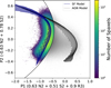 |
Fig. 1 Density distribution of the data (gray) and the selected samples (colored) in refined optical diagnostic (P1–P2) diagram. The blue grids are the photoionization models for SF regions, and the gray grids are the photoionization models for AGNs; each cross corresponds to a unique pair of metallicity and ionization parameter. Both grids are applied a cut so that only the parts that within the middle 98% of the total data along the hidden P3 axis are shown. The definitions of P1 and P2 are in the text. The demarcation line corresponds to fS F = 0.90, which means the maximum contamination to Hα from AGN-ionized regions is 10%. |
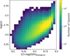 |
Fig. 2 Location of the bins in the metallicity–ionization parameter diagram. Each square represents a bin, and squares are color-coded by the number of spaxels in the bin. Bins with fewer than 50 spaxels are not shown in this diagram. |
2.3 Binning and stacking
To measure metallicities using the direct method, detecting the faint auroral lines, particularly [O III]λ 4363, is a critical requirement. Because auroral lines can be a hundred times fainter than the strong lines, we enhanced the S/N of the spectra by stacking spaxels that were expected to have similar metallicities.
First of all, we estimated the metallicities and ionization parameters of our sample spaxels based on the three strong-line ratios ([N II]/Hα, [S II]/Hα, [O III]/Hβ) using a Bayesian method described by Ji & Yan (2022). The ionization parameter, denoted as U and often presented in logarithm (log(U)), represents the relative strength of the ionizing radiation and is defined as ![Mathematical equation: $\[U=\frac{\phi_{0}}{n_{H} c}\]$](/articles/aa/full_html/2025/11/aa56301-25/aa56301-25-eq4.png) , where ϕ0 is the flux of ionizing photons, nH is the volume density of hydrogen, and c is the speed of light, ensuring that U is a dimensionless parameter. This parameter serves as an essential tracer of the ionizing state within the spatially resolved region. In this work, we generate CLOUDY models with a metallicity grid sampling the following values in [O/H]: −1.3, −0.7, −0.4, 0, 0.3, and 0.5, and an even ionization parameter grid from −4 to −0.5 with a spacing of 0.5 in log(U). Both the metallicity and ionization parameter grids are interpolated to 100 values. Each metallicity-ionization parameter combination (a node in the model of Fig. 2) will provide a set of line ratios for [N II]/Hα, [S II]/Hα, and [O III]/Hβ according to the emissivities of emission lines. With the input of the line ratios from data, the probability distribution functions (PDFs) could be calculated using Bayesian inference, simultaneously for the metallicity and log(U). Details for the Bayesian method are described by Blanc et al. (2015).
, where ϕ0 is the flux of ionizing photons, nH is the volume density of hydrogen, and c is the speed of light, ensuring that U is a dimensionless parameter. This parameter serves as an essential tracer of the ionizing state within the spatially resolved region. In this work, we generate CLOUDY models with a metallicity grid sampling the following values in [O/H]: −1.3, −0.7, −0.4, 0, 0.3, and 0.5, and an even ionization parameter grid from −4 to −0.5 with a spacing of 0.5 in log(U). Both the metallicity and ionization parameter grids are interpolated to 100 values. Each metallicity-ionization parameter combination (a node in the model of Fig. 2) will provide a set of line ratios for [N II]/Hα, [S II]/Hα, and [O III]/Hβ according to the emissivities of emission lines. With the input of the line ratios from data, the probability distribution functions (PDFs) could be calculated using Bayesian inference, simultaneously for the metallicity and log(U). Details for the Bayesian method are described by Blanc et al. (2015).
Spaxels with similar metallicities and ionization parameters are likely to correspond to star formation (SF) regions that share comparable properties, such as electron temperature and density. Compared to the commonly used empirical strong-line method (e.g., O3N2 and N2 from Marino et al. 2013, N2S2Hα from Dopita et al. 2016), we used the same line ratios as theirs to measure metallicity. However, different from an equation that is straightforward to calculate metallicities, the Bayesian inference does not provide an equation but only the probability. The metallicities of the data are derived from their posterior distribution-weighted mean values.
We binned the spaxels based on these Bayesian method-derived metallicities and ionization parameters, using a bin size of 0.05 × 0.05 dex. For convenience, we abbreviate the bin with [O/H] between a and a + 0.05, and log(U) between b and b + 0.05 as ![Mathematical equation: $\[\left(\mathrm{Z}_{a}^{a+0.05}, \log (\mathrm{U})_{b}^{b+0.05}\right)\]$](/articles/aa/full_html/2025/11/aa56301-25/aa56301-25-eq5.png) in this work. Figure 2 illustrates the number of spaxels within each bin, and we only focus on bins containing more than 50 spaxels. We suspect that bins with an insufficient number of spaxels may not yield a reliable measurement of auroral lines, even after stacking.
in this work. Figure 2 illustrates the number of spaxels within each bin, and we only focus on bins containing more than 50 spaxels. We suspect that bins with an insufficient number of spaxels may not yield a reliable measurement of auroral lines, even after stacking.
To carry out stacking, we pulled out each individual spectrum and its uncertainties from the MaNGA DRP LOGCUBE files. Then we corrected for its reddening effect caused by the Milky Way, assuming the reddening map of Schlegel et al. (1998) and the reddening law following O’Donnell (1994). Since different galaxies have different redshifts, and there are velocity offsets for different spaxels in the same galaxies (which are both provided by MaNGA DAP), we shifted the spectra back to a logarithmic wavelength grid in the rest frame following the rebinning process described by Lee et al. (2024). In this process, the flux was proportionally allocated to new pixels in the wavelength axis, conserving the flux.
Finally, we normalized each spectrum by the mean flux between 6000–6100 Å, a relatively feature-free region, and average all the spectra in the same bin to construct the stacked spectrum. The effect of normalization and stacking on line flux ratios can be expressed as
![Mathematical equation: $\[\frac{f_{\lambda_1}}{f_{\lambda_2}}=\frac{\Sigma_i \frac{f_{i \lambda_1}}{C_i}}{\Sigma_i \frac{f_{i \lambda_2}}{C_i}}=\frac{\Sigma_i \frac{f_{i \lambda_1}}{f_{i \lambda_2}} \frac{f_{i \lambda_2}}{C_i}}{\Sigma_i \frac{f_{i \lambda_2}}{C_i}},\]$](/articles/aa/full_html/2025/11/aa56301-25/aa56301-25-eq6.png) (4)
(4)
where fλ1 and fλ2 are observed flux from wavelength λ1 and λ2 in a normalized spectrum, i is the ith spaxel stacked, and C is the “weight” for normalization. We also test using the median value instead of the mean as the stacking results. Table 1 shows the difference in the fluxes of strong lines between median stacks and mean stacks. For strong lines, the differences are around 1% even for those bins with the largest deviations. For auroral lines, all the residuals of median stacks minus mean stacks are smaller than the uncertainties. We believe that using mean stack or median stack would yield equivalent results for this study.
Statistical differences between median stack and mean stack for strong lines.
2.4 Stellar continuum subtraction
After getting high-S/N spectra, the stellar continuum needs to be subtracted to measure the emission lines. In this work, we use the stellar templates from MaStar Hierarchical Clustering (hereafter MaStarHC, described by Abdurro’uf et al. 2022). MaStarHC was generated from MaStar (Yan et al. 2019), which is a well-calibrated empirical stellar library that used the same set of spectrographs as the MaNGA survey. Thus, the templates have the same wavelength coverage and a similar spectral resolution as MaNGA (R ~ 1800). To achieve better stellar continuum subtraction, we applied the penalized pixel-fitting (pPXF, Cappellari 2023) to the stacked spectra. By fitting multiple templates to an observed spectrum, pPXF allows for the robust extraction of stellar kinematics and stellar population properties.
We followed the continuum modeling and line-fitting procedure adopted by MaNGA DAP, which separates the determination of stellar kinematics from stellar continuum and emission lines fitting. First, we conducted a fitting for the stacked spectrum, only using the stellar templates with an additive Legendre polynomial to determine stellar kinematics. In Section 7 of Westfall et al. (2019), they discuss the influence of different orders of polynomials. We followed their conclusions and used the eighth order. As an additive Legendre polynomial will change the depth of absorption or emission feature, this result is not recommended for use as the stellar continuum of the spectrum. However, it can produce reliable measurements for stellar kinematics, both the velocity offset between the spectra and the templates and the velocity dispersion of the spectra. Masking out regions with emission lines, we did the fitting and masked the pixels with residuals exceeding 3 σ. Then we iterated the above procedure to convergence and got the stellar kinematics. Fixing the stellar kinematics inputs, we did another fitting using both the stellar templates and the Gaussian emission line templates. In this fitting, the input spectrum is still the stacked spectrum. For emission lines, we fixed the velocity offset of all the lines. However, their amplitudes are free. There are exceptions for several sets of doublets, where their line ratios are fixed. We tested the effect of using different orders of multiplicative polynomials and set an eighth-order multiplicative Legendre polynomial for this fitting, following the MaNGA DAP. The multiplicative Legendre polynomials can provide precise subtraction by mimicking the impact of dust effect on stellar continuum (Cappellari 2017).
Fig. 3 demonstrates our stacking and stellar continuum subtraction procedures for [S II]λλ 4069,4076 (top-left panel), [O II]λλ 7320,7330 (top-right panel), [S III]λ 6312 (mid-left panel), [O III]λ 4363 (mid-right panel), and [N II]λ 5755 (bottom panel) from one bin which has the strong-line-derived [O/H] range of −0.15~−0.10 and the ionization parameter range of −2.85~−2.80. In each panel, the top row shows a representative spectrum from MaNGA, where the weak auroral lines are “hidden” in the noise that are shown as shaded regions. After stacking spectra in this bin (see Section 2.3), the blue line in the middle row gets vastly increased in the S/N and becomes much smoother. Thus, the auroral lines can be detected. For comparison, the red line is the best-fitting stellar continuum component from the second time fitting of pPXF, which successfully subtracted the stellar continuum while leaving the emission lines emitted by ionized gas regions. The bottom row shows the residuals for the stacking spectrum after stellar continuum subtraction. The auroral lines are clearly visible, at which point the processing of the entire spectrum is complete, and we have obtained emission lines with high S/Ns.
The goodness of fit for the pPXF fitting is indicated by the reduced ![Mathematical equation: $\[\chi^{2}(\chi_{reduced}^{2})\]$](/articles/aa/full_html/2025/11/aa56301-25/aa56301-25-eq7.png) , while
, while ![Mathematical equation: $\[\chi_{reduced}^{2} \simeq 1\]$](/articles/aa/full_html/2025/11/aa56301-25/aa56301-25-eq8.png) means the fitting uncertainty is reliable. Among the 329 metallicity-ionization parameter bins, we obtain a mean
means the fitting uncertainty is reliable. Among the 329 metallicity-ionization parameter bins, we obtain a mean ![Mathematical equation: $\[\chi_{reduced}^{2}\]$](/articles/aa/full_html/2025/11/aa56301-25/aa56301-25-eq9.png) of ~2.0, which illustrates that the input uncertainties are underestimated. Therefore, we scale the input uncertainties by
of ~2.0, which illustrates that the input uncertainties are underestimated. Therefore, we scale the input uncertainties by ![Mathematical equation: $\[\sqrt{\chi^{2}}\]$](/articles/aa/full_html/2025/11/aa56301-25/aa56301-25-eq10.png) .
.
2.5 Emission line flux measurements
We used a similar fitting method as Yan (2018) to fit the emission lines for the continuum-removed stacked spectrum. For the singlet, we simultaneously fit a linear continuum from two side-bands near the emission line as well as a single Gaussian profile for the emission line, which has a fixed center on its rest-frame wavelength. Subtracting the linear continuum, we can get rid of spectrum skewing due to the potentially limited continuumfitting quality. When fitting an emission line, we selected the Gaussian flux above the linear continuum as the flux measurement of the emission line, as well as chose the uncertainty of the Gaussian fitting, which originates from the uncertainty of stacked spectra, as the uncertainty. For the doublet, we fit two Gaussian profiles and constrain their wavelength centers by the relatively strong line. We also fixed the velocity dispersions of the two lines to be the same.
While dealing with the [O III]λ 4363 measurement, we noticed an emission line near 4359 Å, which makes a double-peak-like feature near [O III] λ 4363. Similar situations were reported in other papers (Curti et al. 2017; Arellano-Córdova & Rodríguez 2020), and it is suspected to be the [Fe II]λ 4359. After verification, we found another [Fe II]λ 4288 line with the same upper energy level as [Fe II]λ 4359, which can also be detected in the stacked spectra. In Fig. 3, they are indicated by vertical gray lines. We are uncertain what affects the flux ratio of [Fe II] lines, but as the metallicity grows, both [Fe II] lines become stronger. It is suggested that there is a fixed line ratio between [Fe II] λ 4288 and [Fe II]λ 4359; however, in the stacked spectra, we do not find the relation between these two line fluxes.
To clear the contamination of [Fe II]λ 4359 line, we used a similar method as Curti et al. (2017). First, we fit a double-Gaussian profile for [Fe II]λ 4359 and [O III]λ 4363, fixing their velocity width to be the same. It is not necessary for [O III]λ 4363 and [Fe II]λ 4359 to have the same width; our fixation is only to make sure both emission lines can be fitted. If the best-fitting velocity width is broader than 5 pixels or two wavelength centers are shifted by more than 2 Å, we can assume [O III]λ 4363 is undetected. For the other case, similar to Andrews & Martini (2013), we classified that [O III]λ 4363 as contaminated if the [Fe II]λ 4359 line flux is ≥0.5 times of the [O III]λ 4363 line flux. After two rounds of selection, 228 of the 329 bins were excluded, and the remaining bins are concentrated in subsolar metallicity regions. We believe that there are many factors other than wavelength that determine the width of emission lines. Therefore, we did not choose to fix the width of [O III]λ 4363 to H γ as done in other works. For the remaining bins, we first subtracted the flux of [Fe II]λ 4359, then fit a single Gaussian profile for [O III]λ 4363, fixing its center as its wavelength, allowing the changes of amplitude and broadening, to finally get the reliable measurement of [O III]λ 4363 line flux.
3 Dust attenuation correction
Dust extinction or attenuation corrections for emission lines are usually done by comparing the observed Balmer decrement with the theoretical Case B value and applying an extinction or attenuation curve (e.g., Cardelli et al. 1989; O’Donnell 1994; Fitzpatrick 1999; Calzetti et al. 2000). However, this straightforward measurement may not be valid for correcting emission lines in observations with kpc-scale spatial resolution, as Ji et al. (2023) states. Since the spatial resolution of MaNGA is ~1–2 kpc, and the typical scale of an SF region is ~10–100 pc, the spectra we obtain could be a mixture of SF regions with DIG (Zhang et al. 2017; Mannucci et al. 2021). And even if we go to smaller scales around 10 pc, we may still see this effect. The issue is that dust extinction is patchy on very small scales; hence, different regions with different line ratios can have different extinctions as evaluated by an effective E(B-V). As a result, not all emission lines share the same amount of extinction. Also, extinction correction curves, for example Fitzpatrick (1999) (hereafter F99), provide a simple extinction correction method, but the actual situations are often more than extinction, so these corrections could be incomplete in explaining attenuation (Salim & Narayanan 2020). One cannot use a single extinction or attenuation curve to correct all emission lines simultaneously.
As a result of the line ratio differences between DIG and H II regions, Ji et al. (2023) pointed out that low ionization lines have a tendency to have less effective attenuation compared to hydrogen recombination lines, at least for MaNGA data. Therefore, our correction process is questionable if we do not consider the potential inconsistency. So far, all the discussions about dust attenuation correction are limited to strong nebular lines. In the case of auroral lines, other methods have not been tried because of the difficulty in detecting them. For [S II] and [O II], because the wavelength intervals between auroral lines and strong lines are large, the dust effect becomes a more serious problem. Malkan (1983) explores the [S II] and [O II] auroral-to-strong line ratios themselves as tracers of dust. However, it is essential to be aware that even a slight difference in line flux measurements could introduce a significant influence on the measurement of electron temperature and metallicity. Consequently, we aim to carefully apply a more accurate method to conduct attenuation correction for these stacked spectra.
Above all, we want to test whether the low-ionization auroral-to-strong line ratios have the same amount of effective attenuation as hydrogen lines. If they have the same tendency as that for strong line ratios, we would like to figure out how different their attenuations are. To conduct the test, we divided each metallicity-ionization parameter bin into nine sub-bins by the Hα/Hβ value of each spaxel from MaNGA DAP, with each sub-bin having one tenth of the number of spaxels of the bin, discarding the first and last 5% to avoid outliers causing offsets by extreme cases. Then, we stacked the spaxels for every subbin and subtract their stellar continuum, following the procedure in Sect. 2.3. We need to have more rigorous spaxel numbers cut to obtain the S/N of the stacked spectra that enable us to detect faint auroral lines in sub-bins. Here, we only chose those bins that contain more than 1000 spaxels so that there are at least 100 spaxels in each sub-bin, and 168 bins satisfy the criterion. We measured the line ratios and uncertainties for [S II], [O II], and [O III] auroral-to-strong lines as well as for Hα/Hβ in every subbin. Since all the sub-bins in one bin have similar metallicities and ionization parameters within a range of 0.05 dex, it can be assumed that they have the same physical properties and intrinsic line ratios. Under these circumstances, the line ratio difference can be attributed to the difference in Balmer decrement, which is expressed as
![Mathematical equation: $\[\begin{aligned}\log \frac{f_{\lambda_1}}{f_{\lambda_2}} & =\log \left(\frac{f_{\lambda_1}}{\mathrm{f}_{\lambda_2}}\right)_{\text {intrinsic }}-0.4\left(\mathrm{~A}_{\lambda_1}-\mathrm{A}_{\lambda_2}\right) \\& =\log \left(\frac{f_{\lambda_1}}{f_{\lambda_2}}\right)_{\text {intrinsic }}-\frac{\mathrm{A}_{\lambda_1}-\mathrm{A}_{\lambda_2}}{\mathrm{~A}_{\mathrm{H} \alpha}-\mathrm{A}_{\mathrm{H} \beta}} \log \left(\frac{f_{H \alpha} / f_{H \beta}}{2.86}\right) \\& =\log \left(\frac{f_{\lambda_1}}{f_{\lambda_2}}\right)_{\text {intrinsic }}-\mathrm{m}_{\lambda_1, \lambda_2} \log \left(\frac{f_{H \alpha} / f_{H \beta}}{2.86}\right),\end{aligned}\]$](/articles/aa/full_html/2025/11/aa56301-25/aa56301-25-eq12.png) (5)
(5)
where λ1 and λ2 are the wavelength of emission lines, and Aλ is the attenuation at wavelength λ. We carry out a linear regression fit for each of the nine data points in one bin, and the slope will be the m in Eq. (5), which indicates the attenuation difference of λ1 and λ2 relative to Hα and Hβ.
When fitting, we simultaneously considered the uncertainties of Balmer line ratios and the uncertainties of the auroral-to-strong line ratios. We followed the method of Tremaine et al. (2002), which gives a likelihood measurement of
![Mathematical equation: $\[\begin{aligned}\ln~ F_{likelihood, i} & =-0.5 \chi_i^2 \\& =-0.5\left(y_i-m x_i-b\right)^2 /\left(m^2 \sigma_{x_i}^2+\sigma_{y_i}^2+\sigma_0^2\right)\end{aligned}\]$](/articles/aa/full_html/2025/11/aa56301-25/aa56301-25-eq13.png) (6)
(6)
when carrying out a linear fitting, y = mx + b. σx, σy, and σ0 are the uncertainties of the x and y axes, and the intrinsic scatter of the y axis, respectively. σx and σy were computed by the error propagated from each single spectrum. The intrinsic scatter should be the same for all the data during the fit, and we cannot separate it directly from σy. Firstly, we set σ0 = 0 and minimized the χ2 using the minimize function from SciPy once. After that, we set σ0 as an unknown, together with slope and intercept, and set the first-time calculated σ0 as the new initial guess. Then, we applied the minimize function again. This method originates from Ji et al. (2023), but we make an improvement so that no iteration is needed.
In Fig. 4, the fitting results of one bin are shown. The red lines are our fitting results using the method described above. For comparison, we also show the best fit using the F99 slope but allowing the intercept to change, which is shown in green. While we consider the x and y uncertainties simultaneously, the uncertainties of the Balmer decrement are small. It is clearly seen that although there are fairly large uncertainties for auroral-to-strong line ratios, our fits match the data points better.
After we got all the fitting results, histograms were generated – see Fig. 5 – to demonstrate the distributions of the relative attenuation for [S II], [O II], and [S III]. For [O II] and [S II], it is clear that, although there are large scatters, the slope distributions of the sub-bins deviate from the slopes calculated from F99 (dashed green line). Using the F99 curve with the same E(B-V) as derived from Balmer decrement would overcorrect the attenuation for these two ion species in our data. This is consistent with the trends displayed by the low-ionization strong line ratios shown by Ji et al. (2023). For [S III] (right panel of Fig. 5), the median slope is similar to that of F99, also consistent with the trends displayed by high-ionization strong line ratios shown by Ji et al. (2023). The cause of the different slopes could either be that the extinction curve needs modification, or the attenuations seen by different ions are different. As argued by Ji et al. (2023), the latter is a much more likely interpretation.
For every bin, including those that have fewer than 1000 spaxels, we applied this median slope correction to correct the auroral-to-strong line ratios for [O II] and [S II]. The best-fit ratios at Hα/Hβ =2.86 were taken as the intrinsic, unattenuated ratios. Different metallicty-ionization parameter bins would have different intrinsic ratios. We subtracted the intrinsic ratios from the observed ratios, merged all bins together, and plotted them against Hα/Hβ to check for the dependence on Balmer decrement, before and after dust correction. This is shown in Fig. 6, where purple contours denote no corrections, green contours denote F99 corrections, and red contours denote our corrections. Three levels mean 68%, 95%, and 99% of the data points. It is evident that F99 corrections will overcorrect the attenuation by dust and leave an opposite residual dependence, while our correction yields a close-to-zero residual dependence.
It is possible that the relative levels of attenuation for low-ionization ions compared to hydrogen may have a dependence on ionization parameter and metallicity. We also inspected the metallicity and ionization parameters dependence of slopes for [S II], [O II], and [S III] auroral-to-strong line ratios, but they have large uncertainties, and no significant dependence has been found. We further inspected the strong line ratio [S II]λλ 6716,6731/[O II]λλ 3726,3729, whose median slope, uncertainties, and standard deviation are also shown in Table 2. As a strong line ratio, [S II]λλ 6716,6731/[O II]λλ 3726,3729 exhibits a small standard deviation, and all of the slopes are shallower than the F99 correction slope. Plotting the dependence of [S II]λλ 6716,6731/[O II]λλ 3726,3729 slopes with two binning parameters, we find that the relative attenuations have a strong correlation with the ionization parameters but are less correlated with metallicities, surprisingly. This suggests that high ionization parameter regions are dustier, and we may need to consider the correlation between relative attenuation and ionization parameter when correcting for dust for low ionization auroral lines.
For [O III]λ 4363 which represents high ionization zones, due to its faintness in most bins and the minor difference in wavelength for the auroral line and the strong line, we simply apply the F99 correction, assuming this line ratio obeys the same extinction law as Balmer lines. For [S III] lines, which represent intermediate ionization zones, we try the same fitting method. Different from the low ionization lines, the absolute intensities of [S III] lines appear to be weaker for both the auroral and the strong lines, and the [S III]λ 6312 is relatively weak and adjacent to [O I]λ 6300. The right panel of Fig. 5 shows that the slope displayed by [S III] auroral-to-strong line ratio is similar to that of F99, deviating by only 1 sigma. Thus, we also apply F99 to [S III]λ 6312. For [N II]λ 5755, as there are few data points to be considered, and the wavelengths of auroral and strong lines are close, we also use F99.
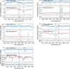 |
Fig. 3 Spectra of [S II] auroral lines (top left), [O II] auroral lines (top right), [S III] auroral line (mid left), [O III] auroral line (mid right), and [N II] auroral line (bottom left) from a sample bin |
![Mathematical equation: $\[\left(\mathrm{Z}_{-0.15}^{-0.10}, \log (\mathrm{U})_{-2.85}^{-2.80}\right)\]$](/articles/aa/full_html/2025/11/aa56301-25/aa56301-25-eq11.png)
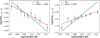 |
Fig. 4 Auroral-to-strong line ratio of [S II] (left) and [O II] (right) versus normalized Balmer decrement (HαHβ2.86) in one randomly chosen metallicity-ionization parameter bin, both in logarithm space. Each data point represents the line ratio of a sub-bin that is constructed by spaxels with similar Balmer decrements. The error bars describe the uncertainties of line ratios. The green line is the F99 correction relation with Rv = 3.1, which is generally steeper than the data distribution. The red line is our fitting for these data points, which considers both the x and y axes uncertainties simultaneously. |
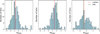 |
Fig. 5 Slopes of relative attenuation distribution in the blue histograms of the linear fitting for [S II] λλ 4069,4076/[S II] λλ 6716,6731 (left) and [O II] λλ 7320,7330/[O II] λλ 3726,3729 (middle), and [S III] λ 6312/[S III] λλ 9068,9531 (right) of all the sub-bins. The green lines represent the slopes of relative attenuation from F99, and the red lines represent the median slopes of 168 bins. The values of median slopes are presented in Table 2. |
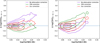 |
Fig. 6 Relation between [O II] (left) and [S II] (right) auroral-to-strong line ratios differences and log(Hα/Hβ) from all the sub-bins, a total number of 1512. The line ratio differences mean the actual auroral-to-strong line ratios minus the intrinsic auroral-to-strong line ratios given by the intercept of the best-fit line in each bin. The purple contours represent the density distribution of data without any correction. The green contours represent data after a F99 correction with RV = 3.1. The red contours represent data after our correcting method described in this section. The contour levels represent 68%, 95%, and 99% of all the data points. The dashed blue lines are horizontal. A horizontal distribution is expected for the correct attenuation correction, as there should be no residual dependence on the Balmer decrement. |
Statistical properties of relative attenuation.
4 Results
4.1 Electron density
We measured the electron temperature using auroral-to-strong line ratios from different ion species representing different ionization zones. The ionization energy of O+ is high, so lines from O2+ represent regions that are highly ionized. O0 and S0 have ionization energy close to H0 so lines from O+ and S+ represent low ionization zones. Since S+’s ionization energy is between that of H0 and O+, [S III] can be a good tracer for intermediate ionization zones. However, in most works applying the direct method to SDSS Legacy data, the intermediate ionization zone is not considered because either the wavelength coverage was insufficient for [S III]λλ 9069,9533 or the relative intensity of [S III]λ 6312 was much weaker than its neighbor, [O I]λ 6300. Nevertheless, MaNGA enables us to measure both [S III]λ 6312 and [S III]λλ 9069,9533 in this paper.
We used PYNEB version 1.1.18 (Luridiana et al. 2015; Morisset et al. 2020) to estimate the electron temperature and density of the stacked spectrum from each metallicity-ionization parameter bin. The getCrossTemDen function in PYNEB enables us to input two sets of line ratios (one density indicator and one temperature indicator) and obtain the electron density and temperature simultaneously based on the five-level atomic structure originating from De Robertis et al. (1987). For transition probability and collisional strength, we use the newest default atomic data from PYNEB (‘PYNEB_23_01’).
For electron density, we chose the [S II] 6731/[S II] 6716 as the indicator. The doublet has critical densities of ≃1400 and 3600 cm−3 at Te = 104 K, where the collisional and radiative de-excitation reaches an equilibrium. There are other density indicators such as [O II]λλ 3726,3729, [Ar IV]λλ 4711,4740, and even [S II]λλ 4069,4076 and [O II]λλ 7320,7330, but the latter two are too faint as they are auroral lines, and [Ar IV]λλ 4711,4740 is also too faint, although it represents densities in high ionization zones and is worth examining. [O II] 3726/[O II] 3729 has a higher critical density than [S II] doublet, but we do not use it as the two lines are poorly resolved. In Fig. 7, we present the histogram of densities derived from [S II]. Here we assume the electron temperature is 104 K, since the doublet line ratios are almost independent of temperature when densities are low (Nicholls et al. 2020).
4.2 Electron temperature
We input the auroral-to-strong line ratio for electron temperature for all five ion species. As the densities typically have values of ne < 150 cm−3, the density variation will not affect their temperature computation for [O II], [N II], and [S III]. However, the lower critical densities of [O II] and [S II] may lead to a significant difference in the temperature measurement with minor changes in density. The uncertainties of temperatures are computed via Monte Carlo simulations. As we know the uncertainties of auroral-to-strong line flux ratio (theoretical error propagation with error computed in Section 2.5), we generated 1000 simulated values of the line ratio following a Gaussian distribution whose σ is the line ratio uncertainty for each pair of line ratio in each bin. Among the 1000 temperature measurements we obtained, the 16% and 84% values were set as the uncertainty range of the electron temperature.
Fig. 8 presents the Te versus Te between different ionization species. Focusing on temperatures of low-ionization ions, shown in the three upper panels, we first discover that Te [O II] follow a different relation with metallicities compared to the other two Te. When the metallicity is low, which corresponds to deep-color dots, Te [O II] decreases with the increasing strong-line metallicity of the bin. This is the same as what Te [S II] and Te [N II] obey. However, Te[O II] stops decreasing at high metallicity and shows an upturn trend. We exclude the possibility of improper emission line fitting after checking the spectra of individual bins. Details of this abnormal phenomenon are discussed in detail by Peng et al. in prep, who argue Te[O II] is not qualified to represent the low ionization zone due to its offset from the correlation of electron temperature and metallicity. In the upper left panel, Te [S II] and Te[O II] are relatively consistent and close to the 1:1 line except that they are offset when metallicity is high, and they exhibit a larger dispersion when metallicity is low. However, the data do not stick to the 1:1 line in the upper middle and upper right panels. In both panels, Te [N II] shows uncertainties more than 3000 K at lower metallicity, much larger than Te [S II] and Te [O II]. Although Te [N II] is thought to be a good temperature indicator for low-ionization zones owing to its small scatter and the minor effect of dust on it (Berg et al. 2015; Rickards Vaught et al. 2024), Te [N II] has a larger uncertainty than those of Te[O II] and Te [S II]. In the BOSS spectrographs, the redshifted [N II]λ 5755 happens to be located near the junction between the blue and red cameras, which makes the residual near the emission line noisy (see Fig. 2). Therefore, [N II]λ 5755 is detected in fewer bins than other auroral lines. The large uncertainties of Te [N II] prevent us from further analyzing [N II]λ 5755/[N II]λ 6584. As a result, we can only set the Te [S II] as the low ionization temperatures.
When it comes to intermediate and high ionization zones, we get fewer data points, mainly concentrating on low-metallicity and relatively high ionization parameter bins. Te [O III] are uniformly higher than Te [S III], shown in the lower left panel. This trend was studied in Binette et al. (2012), and they suggested that this may be caused by metallicity inhomogeneity, a κ-distribution of electron energy, or shock wave. Compared with low ionization lines, Te [O III] and Te [S III] tend to be less dispersed when the binning metallicity and ionization parameter change. Another noteworthy point is that we do not have extremely high Te [O III] (typically over 15 000 K), which can probably be attributed to the averaging effect of stacking and better removal of the contamination of [Fe II]λ 4359. Comparing Te [S III] to Te [S II] in the middle right panel, we find that [S II] auroral-to-strong line ratios will derive higher temperature than [S III], contrary to other literature and some empirical relations (Berg et al. 2020; Zurita et al. 2021). But this can be consistent with the theoretical expectation of the rising temperature in the partially ionized zones. If these two Te are fitted linearly, the slope will be shallower than 1. For Te [O III] versus Te [S II] in the bottom right panel, there are only a few data points due to the difficulties of detecting [O III]λ 4363 and getting rid of [Fe II] contamination. They are located near the 1:1 line with some scatter.
In this work, we do not aim to derive linear relations for each Te versus Te, so we only show the 1:1 dashed red lines. We are also not keen on calibrating t2-t3 relations, which provide a reference for the low (high) ionization temperature once high (low) ionization temperature is derived. The limited quality of some data (e.g., [N II]) and the unclear physics of electron temperatures (e.g., Te [O II]) prevent us from fitting data points linearly. Also, in Fig. 8 we only consider the binning metallicity and not the ionization parameter. The results obtained by conducting a linear fit in this case are incomplete. We will utilize the bins that have electron temperature measurements to compute their metallicity.
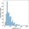 |
Fig. 7 Electron density distribution of all the bins derived from [S II] 6731/[S II] 6716. All the bins are in the low-density limit. |
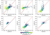 |
Fig. 8 Comparisons between Te derived from [S II], [O II], [N II], [S III], and [O III]. Each dot represents the data from a stacked spectrum of a certain metallicity–ionization parameter bin. The gray error bars correspond to 1 σ uncertainties of the temperature measurements. The dashed red line in each panel shows the 1:1 line. The dashed gray, orange, cyan, and black lines represent previous T–T relations from Zurita et al. (2021) (Z21), Berg et al. (2020) (B20), Méndez-Delgado et al. (2023a) (MD23), and Garnett (1992) (G92). The color of each dot represents its theoretical strong-line metallicity. |
4.3 lonic abundance
We computed the ionic abundance using the getIonAbundance function in PYNEB, which is a Python version of nebular.ionic. Since we know the electron temperature, electron density, and nebular line flux relative to the hydrogen recombination lines, for example, Hβ, the abundance of a certain ion can be calculated. The uncertainty measurement for ionic abundance is propagated from the uncertainties of electron temperature (see Section 4.2). We ignored the uncertainty of electron density as the [S II] doublet are strong lines with very high S/N and the bins are in the low-density limit.
In the computation of the abundance of an element, applying the ionization correction factor (ICF) is essential for accurately determining total elemental abundance from only two observed ionic ratios. Pérez-Montero (2017) lists the details of how to calculate ICF for each species, and we here applied
![Mathematical equation: $\[I C F\left(O^{+}+O^{2+}\right)=1+\frac{y^{2+}}{y^{+}}\]$](/articles/aa/full_html/2025/11/aa56301-25/aa56301-25-eq14.png) (7)
(7)
and
![Mathematical equation: $\[I C F\left(S^{+}+S^{2+}\right)=\left[1-\left(\frac{O^{2+}}{O^{+}+O^{2+}}\right)^\alpha\right]^{-1 / \alpha},\]$](/articles/aa/full_html/2025/11/aa56301-25/aa56301-25-eq15.png) (8)
(8)
where y+ and y2+ represent the abundance of He+ and He2+. We only applied Eq. (7) for oxygen if He II 4686 Å could be detected. Otherwise, we assumed that
![Mathematical equation: $\[\frac{\mathrm{O}^{+}+\mathrm{O}^{2+}}{\mathrm{H}^{+}}=\frac{\mathrm{O}}{\mathrm{H}}\]$](/articles/aa/full_html/2025/11/aa56301-25/aa56301-25-eq16.png) (9)
(9)
and did not apply ICF for oxygen as not enough high-energy ionizing photons were present to produce He2+ and O3+. For sulfur, the way to calculate the ICF was initially proposed by Stasińska (1978), and we followed Dors et al. (2016) in choosing α = 3.27. However, some bins had both S+ and S2+ abundance measurements but do not have O2+ abundance. We checked the ICF for measurable bins, and all of them concentrate in the range from 0.99 to 1.03. We then assumed that ICF has an effect of less than 3% for the final results, and used the default ICF = 1 for those bins that do not have O+ or O2+ abundance measurements.
With the correction from ICF, we can derive the total abundance of oxygen and sulfur. Figs. 9 and 10 demonstrate the ionic abundance of S+, S2+, O+, and O2+ across their total abundance we measured. In Fig. 9, the scatter plots reveal the relationship between the ionic abundance of S+ and S2+, both showing positive correlations consistent with expectations, and S2+ having a more linear relation while S+ showing more scatter. In the bottom panel, the S2+/S+appears to be almost independent of total abundance change, while S2+ are more abundant than S+. Conversely, Fig. 10 illustrate the ionic abundances of O+ and O2+. For the O2+, we apply Te [O III]. Since we do not understand why Te [O II] would increase at high metallicity, we also select Te [S II] to calculate the O+ abundance. O+ abundances are positively correlated with the total abundance, while O2+ does not have a significant correlation with the total abundance. As a result, their ratios exhibit a negative correlation with the total abundance. When 12+log(O/H) > 8.2, most of the bins have more O+ than O2+. It is shown in other literature that this ratio will decrease to less than −1.0 at a higher metallicity (Curti et al. 2017). But in our sample, the [O III] detection limits our upper boundary of total abundance measured from the direct method. Data points in both figures are color-coded by Te [S II]. With the increasing abundances, electron temperatures decrease for both S and O.
We compared the total abundances of oxygen and sulfur derived from our measurements with those obtained using the theoretically calibrated method, which we used to bin the spaxels. Here, we used the same assumption as in Ji & Yan (2022) for the solar abundance of oxygen, that is 12+log(O/H)⊙ = 8.69, originating from Grevesse et al. (2011), and a 0.22 dex deduction due to the depletion into dust. For sulfur, we apply 12+log(S/H)⊙ = 7.15 following Asplund et al. (2009). Results for metallicity measurements are shown in Fig. 11. The left panel displays the relationship between the abundance of oxygen (12+log(O/H)direct) and the difference between log(O/H) derived from the direct method and their binning metallicities, color-coded by the ionization parameter of each bin. The median value of the difference between direct metallicity and theoretical strong-line metallicity is −0.09 dex. The right panel illustrates a similar comparison for sulfur, showing the total abundance of sulfur (12+log(S/H)direct) against the differences between the two methods. The median of their difference is also −0.09 dex. In Kewley & Ellison (2008), the theoretical-calibrated metallicity and empirical-calibrated metallicity have more than 0.5 dex of difference. Compared with these results, the differences we obtain are relatively small. Both panels are color-coded by the binning ionization parameters, and they exhibit a strong correlation with the total abundance difference. Most of the data points above the horizontal lines are bins with low ionization parameters, and the direct metallicities we obtain are getting smaller compared to the strong-line metallicities with increasing ionization parameters. This phenomenon illustrates that the two methods may carry different systematic errors in their dependence on ionization parameters.
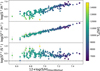 |
Fig. 9 Abundance of S+ (top panel), S2+ (middle panel), and S2+/S+ (bottom panel) versus total abundance. All the abundances are presented in the form of 12+log(abundance). The uncertainties of abundance measurements are illustrated via the gray error bars, and in the bottom panel, the error bars are calculated via error propagation. The dashed line in the bottom panel demonstrates 12 + log(S2+/H) = 12 + log(S+/H). Data points are color-coded by Te [S II]. |
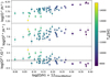 |
Fig. 10 Abundance of O+ (top panel), O2+ (middle panel), and O2+/O+ (bottom panel) versus total abundance. All the abundances are presented in the form of 12+log(abundance). The uncertainties of abundance measurements are illustrated via the gray error bars, and in the bottom panel, the error bars are calculated via error propagation. The dashed line in the bottom panel demonstrates 12 + log(O2+/H) = 12 + log(O+/H). Data points are color-coded by Te [S II]. |
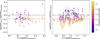 |
Fig. 11 Difference of oxygen (left) and sulfur (right) total abundance derived by the direct method and the theoretical strong-line method versus the total abundance derived by the direct method. The horizontal dashed black lines demonstrate 12 + log(O/H)direct = 12 + log(O/H)StrongLine and 12 + log(S/H)direct = 12 + log(S/H)StrongLine. The horizontal dashed red lines represent the median values of metallicity differences. The gray error bars show the uncertainties of the direct method. Data points are color-coded by the ionization parameters of their bins. |
5 Data-model discrepancy
The discrepancy between metallicity measured using the direct method and that derived from strong lines based on photoionization models has been known before (López-Sánchez et al. 2012; Kewley et al. 2019). However, it is unclear which method is more accurate. Both methods have a number of assumptions behind them, and both can be inaccurate. It is important to compare and contrast them directly in observable space, i.e., line ratio space, to see how large the actual discrepancy is.
The correct photoionization model should be able to simultaneously fit all emission line ratios, including both strong line ratios and auroral-to-strong line ratios. The model we adopt can already simultaneously match the typical [N II]λ 6584/Hα, [S II]λλ 6716,6731/Hα, and [O III]λ 5007/Hβ ratios in most SF regions in MaNGA data. This section will evaluate how well its prediction for auroral-to-strong line ratios matches the data.
5.1 Comparison of the data and models
We compared the observed auroral-to-strong line ratios with the predictions of the photoionization models. The observed data are presented after dust attenuation correction, using F99 for [O III] and [S III] and our specific correction method for [O II] and [S II]. In the comparison, we set the model-based metallicity as the x axis. Both data and model are color-coded by ionization parameter, with two different color bars. The lines with the left color bar show the model, and the dots with the right color bar show the data.
In Fig. 12, we notice that the data tend to have larger scatter at the same metallicity compared to the model. The auroral-to-strong line ratios for [O III] and [S III] exhibit a steeper downward trend with increasing metallicity compared to the model predictions. Except for a few data points, [O III] data are located close to the model. However, it is undetected even at slightly subsolar metallicity. [S III] are almost all below the model. When metallicity is larger than 8.85, they are also undetectable. This is consistent with the commonly seen upper limit of the strong-line method with empirical calibrations, which utilizes metallicity from the direct method. For [O II] and [S II], the observed ratios are roughly consistent with the model in low-metallicity regimes, with [O II] having smaller values and [S II] exhibiting a steeper downward trend. However, in high-metallicity regimes, [O II] shows a significant upturn, which contradicts model predictions. We do not yet have an explanation for this. In contrast, [S II] decreases rapidly when the metallicities are high and are distributed far below the model grids. These trends are independent of dust correction. Attributing the upturn of [O II] and the steep downturn of [S II] to dust attenuation correction would require unrealistically large Rv values.
Fig. 12 also shows the trends of ionization parameters of the data and the model. For the model, auroral-to-strong line ratios slightly increase with increasing ionization parameters at fixed metallicity. Notably, this correlation is reversed for [S III] and [O III] when the model reaches its highest metallicity, which may be due to the extrapolation effect since the ionizing SEDs have an upper limit of 2 times solar metallicity (see Sect. 2.1). Observed data, however, exhibit a more complicated dependence on ionization parameters. Interestingly, [S II] demonstrates an inverse dependence on ionization parameters at fixed metallicity. However, the line ratios of the other three species tend to increase with rising ionization parameters. This divergence shows the complexity between ionization states and emission line intensities, suggesting that the current model does not capture all the physical effects in real H II regions.
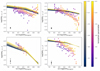 |
Fig. 12 Observed auroral-to-strong line ratios and CLOUDY-generated auroral-to-strong line ratios plotted as functions of binning metallicities for [O II] (upper left), [S II] (upper right), [O III] (lower left), and [S III] (lower right). Lines in the panels represent the data generated by CLOUDY and are color-coded by ionization parameters (the left color bar). Dots in the panels represent the observed data and are also colored by ionization parameters (the right color bar). In the lower left corner of each panel, the black error bar shows the median uncertainty of the observed data. Observed data have a significant offset from the models. |
5.2 Discussion
There are a number of possible reasons that could explain this inconsistency between the data and the model. First, CLOUDY photoionization model is a 1D model. The assumption of uniform or smooth density distribution is unrealistic. In reality, density fluctuations (Méndez-Delgado et al. 2023a), temperature fluctuations (Peimbert 1967), scattering by dust, and contamination by DIG can all make the resulting line ratios different from theoretical predictions. We need more sophisticated 3D modeling incorporating realistic density fluctuations to fully reproduce the observed emission line ratios (e.g., Jin et al. 2023).
Not only do the models need to be improved, but there is also a need to obtain better data to test the models. Temperature fluctuation in the SF regions contributes to the auroral-to-strong line ratio measurement. Since the CELs are generally more sensitive to temperature than the hydrogen recombination lines, and the faintness of auroral lines makes them unlikely to be detected in low-temperature zones, the auroral-to-strong line ratios are often biased to a higher value than the average. As a result, the larger fluctuation will result in a significant overestimation of electron temperatures and underestimation of abundances (Garnett 1992; Peimbert et al. 2017; Méndez-Delgado et al. 2023b; Chen et al. 2023). In the previous studies that used selected H II regions, this effect has a systematic influence, because they may exclude H II regions with lower temperature and result in a low metallicity. This has been improved in our stacked spectra, since the stacked spectra yield the average auroral-to-strong line ratio. Still, this effect may bias the temperatures to higher values than the actual average temperature, and result in a slightly lower direct metallicity than the strong-line metallicity.
To better understand the discrepancies, there is still a need for more high-resolution data targeting nearby individual SF regions. Only after careful observation to obtain the distributions of auroral-to-strong line ratios in these SF regions can we gain a deeper understanding of the chemical evolution in these SF regions and what improvements the photoionization models should make. With the next generation of surveys like SDSS-V/LVM (Drory et al. 2024) and AMASE-P (Yan et al. 2020, 2024), we will achieve a better comprehension of the auroral-to-strong line ratios from both data and models. There is also a need for more data for high-metallicity SF regions where auroral lines are detected. With these data, the real picture of [O II] and [S II] can be examined.
5.3 Comparison to previous works
The differences in metallicities derived with different strong-line calibrations result from various factors (Stasinska 2019). For Te-based strong-line methods, calibrations using different data samples and binning methods may give different results, since different data samples may have different biases in sample selection. The results derived from integrated light of galaxies and spatially resolved observations are also not the same. Berg et al. (2015) points out that the development of atomic data may also affect the final result of the direct method, and hence influence the strong-line calibrations. The line ratios used in strong-line methods may have dependence on physical parameters other than oxygen abundance, for example, log(U) and N/O ratios (Kewley & Dopita 2002; Dopita et al. 2016), and this will also cause inconsistencies (see Kewley et al. 2019 for a review). For photoionization model-based strong-line methods, using different photoionization codes (e.g., MAPPINGS, Sutherland et al. 2018) may give different line ratios. Subtle differences in the input assumptions can likewise lead to discrepant results. Not only do these reasons cause the absolute value of metallicity to be different for the same region, the disparities between methods are also different in different regions.
There are previous studies that have compared the direct method metallicity with strong-line metallicity. For empirical strong-line methods, some improvements have been made to ensure consistency with direct metallicities, such as revisiting the empirical relation with more data (Marino et al. 2013), or adding more line ratio pairs when deriving the calibration (Pilyugin & Grebel 2016). Easeman et al. (2024) compared several empirical calibrators with sulfur-based direct methods, and it also shows that most of the empirical calibrators deviate from direct methods by ~0.2 dex when the 12 + log(O/H) ~ 8.8. For photoionization model-based strong-line methods, Pérez-Montero & Díaz (2005) compared direct metallicity with several empirical calibrators and one photoionization model calibrator (McGaugh 1991), finding that the model-based calibrator has 0.2–0.4 dex difference compared to the paper’s new empirical calibrator. Similar discrepancies were also reported in López-Sánchez et al. (2012). Blanc et al. (2015) confirmed that model-based strong-line methods are systematically higher than the direct method for 0.2 dex, and Vale Asari et al. (2016) yielded the deviations of 0.2–0.4 dex. Pérez-Montero et al. (2021) used SDSS single-fiber spectra of a sample of extreme emission line galaxies with 0 < z < 0.49, and the comparison between model-based strong-line metallicity and direct metallicity shows consistency within the uncertainty range (less than 0.1 dex). However, extreme emission line galaxies have different ionizing stellar populations and gas geometry, which makes them not typical in the local universe, and the photoionization models here only cover subsolar metallicities. The requirement of [O III]λ 4363 detection also means the sample may be biased toward those galaxies with a high average electron temperature. Compared with most previous works, the Ji & Yan (2022) model-based strong-line method used in this paper, although still not perfectly aligned with the direct metallicity, presents a generally smaller deviation from the direct metallicity, even when the metallicity is high (~ 0.09 dex). Overall, this strong-line method is considered to be a reliable metallicity measurement for MaNGA galaxies. Peng et al. in prep. will further discuss the scaling relation derived using this method.
6 Summary
We have carried out direct-method metallicity measurements by stacking spectra using IFU datacubes from SDSS-IV MaNGA. We selected about 1.5 million SF spaxels from SDSS-IV MaNGA DR17 and binned them by their metallicities and ionization parameters derived from the photoionization model described by JY20 using strong lines, and assuming that spaxels with the same metallicity and ionization parameters have the same physical condition and intrinsic emission line ratios. Our conclusions are as follows:
In most of the bins, [S II]λλ 4069,4076 and [O II]λλ 7320,7330 can be successfully detected. [S III]λ 6312 can be found in about two thirds of the bins, and [O III]λ 4363 can only be detected in subsolar metallicity bins with relatively high ionization parameters. [Fe II]λ 4359 contaminates [O III]λ 4363 significantly. Therefore, we only chose [O III]λ 4363 measurements after deducting the contamination from bins that can distinguish these two lines. [N II]λ 5755 are detected in a few bins, with large uncertainties because they fall into the wavelength junction of the two channels of the BOSS spectrograph. Using median values to stack produces almost the same result as using mean values to stack;
We applied a data-based dust attenuation correction method for correcting the auroral-to-strong line ratios and find that low ionization lines ([S II], [O II]) have significantly different attenuation from that of hydrogen derived from Balmer decrement. After our correction, the data do not exhibit residual dependence on the Balmer decrement. For high ionization lines and [N II], using the extinction curve of Fitzpatrick (1999) with the overall attenuation derived from the Balmer decrement is sufficient for correcting the reddening effect;
Electron temperatures were measured for [S II], [O II], [N II], [S III], and [O III]. Te [S III] are lower than Te [S II], and Te [O III] are similar as Te [S II] in low-metallicity regimes with scatters;
Ionic abundance for S+, S2+, O+, and O2+ were computed. After considering the ICF, the total abundance of sulfur and oxygen derived from the direct method is systematically lower than the theoretical strong-line metallicity by a median value of −0.09 dex. While still not fully consistent, this deviation is much smaller than the average deviations based on other theoretical metallicity calibrations previously reported. Metallicities derived using this Bayesian strong-line method based on the JY20 model are reliable for MaNGA and MaNGA-like observations with 1–2 kpc spatial resolutions. Scaling relations derived using these more reliable metallicities will be checked in a follow-up paper;
The discrepancy between direct-method metallicity and the strong-line-derived metallicity gets larger at higher ionization parameter. This could have implications for the redshift evolution studies of the mass-metallicity relations, as samples at different redshifts may be biased differently in their ionization parameters;
Comparing our data to the photoionization model, we have ruled out the possibility that the dust effect could have caused the anomaly of [O II] and [S II] auroral-to-strong line ratios when metallicity is high. Observed data present more complex distributions than the model. [S II] and [S III] auroral-to-strong line ratios decrease faster than the model. [O II] auroral-to-strong line ratios exhibit an upturn that does not exist in the model. The observed data show stronger dependence on ionization parameter, and [S II] has an opposite dependence on ionization parameter. The 1D photoionization model could not account for all the auroral-to-strong line ratios while fitting all the strong line ratios.
For future works, we highlight the need to examine the auroral lines in individual SF regions, especially metal-rich SF regions, to better understand the inconsistency of theoretical-calibrated and empirical-calibrated metallicities.
Acknowledgements
We acknowledge the grant support by the National Natural Science Foundation of China (NSFC; grant No. 12373008) and the support by the Research Grant Council of Hong Kong (Project No. 14302522). ZP thanks Ricky Wai Kiu WONG and Yee Ching LAM for useful discussions. RY acknowledges support by the Hong Kong Global STEM Scholar Scheme (GSP028), by the Hong Kong Jockey Club Charities Trust through the project, JC STEM Lab of Astronomical Instrumentation and Jockey Club Spectroscopy Survey System, and by the NSFC Distinguished Young Scholars Fund (grant No. 12425302). Z.S.L. acknowledges the support from Hong Kong Innovation and Technology Fund through the Research Talent Hub program (PiH/022/22GS). XJ acknowledges ERC Advanced Grant 695671 “QUENCH” and support by the Science and Technology Facilities Council (STFC) and by the UKRI Frontier Research grant RISEandFALL. Funding for the Sloan Digital Sky Survey IV has been provided by the Alfred P. Sloan Foundation, the U.S. Department of Energy Office of Science, and the Participating Institutions. SDSS-IV acknowledges support and resources from the Center for High Performance Computing at the University of Utah. The SDSS website is www.sdss4.org. SDSS-IV is managed by the Astrophysical Research Consortium for the Participating Institutions of the SDSS Collaboration including the Brazilian Participation Group, the Carnegie Institution for Science, Carnegie Mellon University, Center for Astrophysics | Harvard & Smithsonian, the Chilean Participation Group, the French Participation Group, Instituto de Astrofísica de Canarias, The Johns Hopkins University, Kavli Institute for the Physics and Mathematics of the Universe (IPMU)/University of Tokyo, the Korean Participation Group, Lawrence Berkeley National Laboratory, Leibniz Institut für Astrophysik Potsdam (AIP), Max-Planck-Institut für Astronomie (MPIA Heidelberg), Max-Planck-Institut für Astrophysik (MPA Garching), Max-Planck-Institut für Extraterrestrische Physik (MPE), National Astronomical Observatories of China, New Mexico State University, New York University, University of Notre Dame, Observatário Nacional/MCTI, The Ohio State University, Pennsylvania State University, Shanghai Astronomical Observatory, United Kingdom Participation Group, Universidad Nacional Autónoma de México, University of Arizona, University of Colorado Boulder, University of Oxford, University of Portsmouth, University of Utah, University of Virginia, University of Washington, University of Wisconsin, Vanderbilt University, and Yale University. Softwares: Starburst99 (Leitherer et al. 1999), CLOUDY (Ferland et al. 2017), pPXF (Cappellari 2023), Astropy (Astropy Collaboration 2022), Numpy (Harris et al. 2020), Matplotlib (Hunter 2007), extinction (Barbary 2016).
References
- Abdurro’uf, Accetta, K., Aerts, C., et al. 2022, ApJS, 259, 35 [NASA ADS] [CrossRef] [Google Scholar]
- Andrews, B. H., & Martini, P. 2013, ApJ, 765, 140 [NASA ADS] [CrossRef] [Google Scholar]
- Arellano-Córdova, K. Z., & Rodríguez, M. 2020, MNRAS, 497, 672 [CrossRef] [Google Scholar]
- Asplund, M., Grevesse, N., Sauval, A. J., & Scott, P. 2009, ARA&A, 47, 481 [NASA ADS] [CrossRef] [Google Scholar]
- Astropy Collaboration (Price-Whelan, A. M., et al.) 2022, ApJ, 935, 167 [NASA ADS] [CrossRef] [Google Scholar]
- Baldwin, J. A., Phillips, M. M., & Terlevich, R. 1981, PASP, 93, 5 [Google Scholar]
- Barbary, K. 2016, extinction v0.3.0 [Google Scholar]
- Belfiore, F., Westfall, K. B., Schaefer, A., et al. 2019, AJ, 158, 160 [CrossRef] [Google Scholar]
- Berg, D. A., Skillman, E. D., Croxall, K. V., et al. 2015, ApJ, 806, 16 [NASA ADS] [CrossRef] [Google Scholar]
- Berg, D. A., Pogge, R. W., Skillman, E. D., et al. 2020, ApJ, 893, 96 [NASA ADS] [CrossRef] [Google Scholar]
- Binette, L., Matadamas, R., Hägele, G. F., et al. 2012, A&A, 547, A29 [NASA ADS] [CrossRef] [EDP Sciences] [Google Scholar]
- Blanc, G. A., Kewley, L., Vogt, F. P. A., & Dopita, M. A. 2015, ApJ, 798, 99 [Google Scholar]
- Brazzini, M., Belfiore, F., Ginolfi, M., et al. 2024, A&A, 691, A173 [NASA ADS] [CrossRef] [EDP Sciences] [Google Scholar]
- Bundy, K., Bershady, M. A., Law, D. R., et al. 2015, ApJ, 798, 7 [Google Scholar]
- Calzetti, D., Armus, L., Bohlin, R. C., et al. 2000, ApJ, 533, 682 [NASA ADS] [CrossRef] [Google Scholar]
- Cappellari, M. 2017, MNRAS, 466, 798 [Google Scholar]
- Cappellari, M. 2023, MNRAS, 526, 3273 [NASA ADS] [CrossRef] [Google Scholar]
- Cardelli, J. A., Clayton, G. C., & Mathis, J. S. 1989, ApJ, 345, 245 [Google Scholar]
- Chen, Y., Jones, T., Sanders, R., et al. 2023, Nat. Astron., 7, 771 [Google Scholar]
- Cowie, L. L., & Songaila, A. 1986, ARA&A, 24, 499 [NASA ADS] [CrossRef] [Google Scholar]
- Curti, M., Cresci, G., Mannucci, F., et al. 2017, MNRAS, 465, 1384 [Google Scholar]
- De Robertis, M. M., Dufour, R. J., & Hunt, R. W. 1987, JRASC, 81, 195 [NASA ADS] [Google Scholar]
- Dopita, M. A., Sutherland, R. S., Nicholls, D. C., Kewley, L. J., & Vogt, F. P. A. 2013, ApJS, 208, 10 [NASA ADS] [CrossRef] [Google Scholar]
- Dopita, M. A., Kewley, L. J., Sutherland, R. S., & Nicholls, D. C. 2016, Ap&SS, 361, 61 [NASA ADS] [CrossRef] [Google Scholar]
- Dors, Jr., O. L., Krabbe, A., Hägele, G. F., & Pérez-Montero, E. 2011, MNRAS, 415, 3616 [NASA ADS] [CrossRef] [Google Scholar]
- Dors, O. L., Pérez-Montero, E., Hägele, G. F., Cardaci, M. V., & Krabbe, A. C. 2016, MNRAS, 456, 4407 [NASA ADS] [CrossRef] [Google Scholar]
- Draine, B. T. 2011, Physics of the Interstellar and Intergalactic Medium (Princeton University Press) [Google Scholar]
- Drory, N., MacDonald, N., Bershady, M. A., et al. 2015, AJ, 149, 77 [CrossRef] [Google Scholar]
- Drory, N., Blanc, G. A., Kreckel, K., et al. 2024, AJ, 168, 198 [NASA ADS] [CrossRef] [Google Scholar]
- Easeman, B., Schady, P., Wuyts, S., & Yates, R. M. 2024, MNRAS, 527, 5484 [Google Scholar]
- Espinosa-Ponce, C., Sánchez, S. F., Morisset, C., et al. 2020, MNRAS, 494, 1622 [Google Scholar]
- Esteban, C., García-Rojas, J., Carigi, L., et al. 2014, MNRAS, 443, 624 [NASA ADS] [CrossRef] [Google Scholar]
- Ferland, G. J., Chatzikos, M., Guzmán, F., et al. 2017, Rev. Mexicana Astron. Astrofis., 53, 385 [Google Scholar]
- Fitzpatrick, E. L. 1999, PASP, 111, 63 [Google Scholar]
- Garnett, D. R. 1992, AJ, 103, 1330 [NASA ADS] [CrossRef] [Google Scholar]
- Grevesse, N., Asplund, M., Sauval, A. J., & Scott, P. 2011, Can. J. Phys., 89, 327 [NASA ADS] [CrossRef] [Google Scholar]
- Harris, C. R., Millman, K. J., van der Walt, S. J., et al. 2020, Nature, 585, 357 [NASA ADS] [CrossRef] [Google Scholar]
- Hillier, D. J., & Miller, D. L. 1998, ApJ, 496, 407 [NASA ADS] [CrossRef] [Google Scholar]
- Hunter, J. D. 2007, Comput. Sci. Eng., 9, 90 [NASA ADS] [CrossRef] [Google Scholar]
- Jenkins, E. B. 1987, in Interstellar Processes, 134, eds. D. J. Hollenbach, & H. A. Thronson, Jr., 533 [Google Scholar]
- Ji, X., & Yan, R. 2020, MNRAS, 499, 5749 [NASA ADS] [CrossRef] [Google Scholar]
- Ji, X., & Yan, R. 2022, A&A, 659, A112 [NASA ADS] [CrossRef] [EDP Sciences] [Google Scholar]
- Ji, X., Yan, R., Bundy, K., et al. 2023, A&A, 670, A125 [NASA ADS] [CrossRef] [EDP Sciences] [Google Scholar]
- Jin, Y., Sutherland, R., Kewley, L. J., & Nicholls, D. C. 2023, ApJ, 958, 179 [NASA ADS] [CrossRef] [Google Scholar]
- Kewley, L. J., & Dopita, M. A. 2002, ApJS, 142, 35 [Google Scholar]
- Kewley, L. J., & Ellison, S. L. 2008, ApJ, 681, 1183 [Google Scholar]
- Kewley, L. J., Nicholls, D. C., & Sutherland, R. S. 2019, ARA&A, 57, 511 [Google Scholar]
- Khoram, A. H., & Belfiore, F. 2025, A&A, 693, A150 [NASA ADS] [CrossRef] [EDP Sciences] [Google Scholar]
- Kroupa, P. 2001, MNRAS, 322, 231 [NASA ADS] [CrossRef] [Google Scholar]
- Lacerda, E. A. D., Cid Fernandes, R., Couto, G. S., et al. 2018, MNRAS, 474, 3727 [Google Scholar]
- Law, D. R., Yan, R., Bershady, M. A., et al. 2015, AJ, 150, 19 [CrossRef] [Google Scholar]
- Law, D. R., Cherinka, B., Yan, R., et al. 2016, AJ, 152, 83 [Google Scholar]
- Lee, M.-Y. L., Yan, R., Ji, X., et al. 2024, A&A, 690, A83 [NASA ADS] [CrossRef] [EDP Sciences] [Google Scholar]
- Leitherer, C., Schaerer, D., Goldader, J. D., et al. 1999, ApJS, 123, 3 [Google Scholar]
- Liang, Y. C., Hammer, F., Yin, S. Y., et al. 2007, A&A, 473, 411 [NASA ADS] [CrossRef] [EDP Sciences] [Google Scholar]
- Lilly, S. J., Carollo, C. M., Pipino, A., Renzini, A., & Peng, Y. 2013, ApJ, 772, 119 [NASA ADS] [CrossRef] [Google Scholar]
- López-Sánchez, Á. R., Dopita, M. A., Kewley, L. J., et al. 2012, MNRAS, 426, 2630 [CrossRef] [Google Scholar]
- Luridiana, V., Morisset, C., & Shaw, R. A. 2015, A&A, 573, A42 [NASA ADS] [CrossRef] [EDP Sciences] [Google Scholar]
- Maiolino, R., & Mannucci, F. 2019, A&A Rev., 27, 3 [NASA ADS] [CrossRef] [Google Scholar]
- Malkan, M. A. 1983, ApJ, 264, L1 [Google Scholar]
- Mannucci, F., Belfiore, F., Curti, M., et al. 2021, MNRAS, 508, 1582 [NASA ADS] [CrossRef] [Google Scholar]
- Marino, R. A., Rosales-Ortega, F. F., Sánchez, S. F., et al. 2013, A&A, 559, A114 [NASA ADS] [CrossRef] [EDP Sciences] [Google Scholar]
- McGaugh, S. S. 1991, ApJ, 380, 140 [CrossRef] [Google Scholar]
- Méndez-Delgado, J. E., Esteban, C., García-Rojas, J., et al. 2023a, MNRAS, 523, 2952 [CrossRef] [Google Scholar]
- Méndez-Delgado, J. E., Esteban, C., García-Rojas, J., Kreckel, K., & Peimbert, M. 2023b, Nature, 618, 249 [CrossRef] [Google Scholar]
- Morisset, C., Delgado-Inglada, G., Sánchez, S. F., et al. 2016, A&A, 594, A37 [NASA ADS] [CrossRef] [EDP Sciences] [Google Scholar]
- Morisset, C., Luridiana, V., García-Rojas, J., et al. 2020, Atoms, 8, 66 [NASA ADS] [CrossRef] [Google Scholar]
- Nicholls, D. C., Kewley, L. J., & Sutherland, R. S. 2020, PASP, 132, 033001 [NASA ADS] [CrossRef] [Google Scholar]
- O’Donnell, J. E. 1994, ApJ, 422, 158 [Google Scholar]
- Osterbrock, D. E., & Ferland, G. J. 2006, Astrophysics of Gaseous Nebulae and Active Galactic Nuclei (University Science Books) [Google Scholar]
- Pauldrach, A. W. A., Hoffmann, T. L., & Lennon, M. 2001, A&A, 375, 161 [NASA ADS] [CrossRef] [EDP Sciences] [Google Scholar]
- Peimbert, M. 1967, ApJ, 150, 825 [NASA ADS] [CrossRef] [Google Scholar]
- Peimbert, A., & Peimbert, M. 2013, ApJ, 778, 89 [NASA ADS] [CrossRef] [Google Scholar]
- Peimbert, M., Peimbert, A., & Delgado-Inglada, G. 2017, PASP, 129, 082001 [NASA ADS] [CrossRef] [Google Scholar]
- Pérez-Montero, E. 2014, MNRAS, 441, 2663 [CrossRef] [Google Scholar]
- Pérez-Montero, E. 2017, PASP, 129, 043001 [CrossRef] [Google Scholar]
- Pérez-Montero, E., & Díaz, A. I. 2005, MNRAS, 361, 1063 [CrossRef] [Google Scholar]
- Pérez-Montero, E., Amorín, R., Sánchez Almeida, J., et al. 2021, MNRAS, 504, 1237 [CrossRef] [Google Scholar]
- Pilyugin, L. S., & Grebel, E. K. 2016, MNRAS, 457, 3678 [NASA ADS] [CrossRef] [Google Scholar]
- Pilyugin, L. S., & Thuan, T. X. 2005, ApJ, 631, 231 [CrossRef] [Google Scholar]
- Rickards Vaught, R. J., Sandstrom, K. M., Belfiore, F., et al. 2024, ApJ, 966, 130 [NASA ADS] [CrossRef] [Google Scholar]
- Rogers, N. S. J., Skillman, E. D., Pogge, R. W., et al. 2021, ApJ, 915, 21 [NASA ADS] [CrossRef] [Google Scholar]
- Salim, S., & Narayanan, D. 2020, ARA&A, 58, 529 [NASA ADS] [CrossRef] [Google Scholar]
- Schlegel, D. J., Finkbeiner, D. P., & Davis, M. 1998, ApJ, 500, 525 [Google Scholar]
- Smee, S. A., Gunn, J. E., Uomoto, A., et al. 2013, AJ, 146, 32 [Google Scholar]
- Stasińska, G. 1978, A&A, 66, 257 [Google Scholar]
- Stasinska, G. 2019, arXiv e-prints [arXiv:1906.04520] [Google Scholar]
- Sutherland, R., Dopita, M., Binette, L., & Groves, B. 2018, MAPPINGS V: Astrophysical plasma modeling code, Astrophysics Source Code Library [record ascl:1807.005] [Google Scholar]
- Tremaine, S., Gebhardt, K., Bender, R., et al. 2002, ApJ, 574, 740 [NASA ADS] [CrossRef] [Google Scholar]
- Vale Asari, N., Stasińska, G., Morisset, C., & Cid Fernandes, R. 2016, MNRAS, 460, 1739 [NASA ADS] [CrossRef] [Google Scholar]
- Veilleux, S., & Osterbrock, D. E. 1987, ApJS, 63, 295 [Google Scholar]
- Vogt, F. P. A., Dopita, M. A., Kewley, L. J., et al. 2014, ApJ, 793, 127 [NASA ADS] [CrossRef] [Google Scholar]
- Wake, D. A., Bundy, K., Diamond-Stanic, A. M., et al. 2017, AJ, 154, 86 [Google Scholar]
- Westfall, K. B., Cappellari, M., Bershady, M. A., et al. 2019, AJ, 158, 231 [Google Scholar]
- Yan, R. 2018, MNRAS, 481, 476 [NASA ADS] [CrossRef] [Google Scholar]
- Yan, R., Bundy, K., Law, D. R., et al. 2016a, AJ, 152, 197 [Google Scholar]
- Yan, R., Tremonti, C., Bershady, M. A., et al. 2016b, AJ, 151, 8 [Google Scholar]
- Yan, R., Chen, Y., Lazarz, D., et al. 2019, ApJ, 883, 175 [Google Scholar]
- Yan, R., Bershady, M. A., Smith, M. P., et al. 2020, SPIE Conf. Ser., 11447, 114478Y [NASA ADS] [Google Scholar]
- Yan, R., Bershady, M. A., Chattopadhyay, S., et al. 2024, SPIE Conf. Ser., 13096, 130967S [Google Scholar]
- Zhang, K., Yan, R., Bundy, K., et al. 2017, MNRAS, 466, 3217 [NASA ADS] [CrossRef] [Google Scholar]
- Zurita, A., Florido, E., Bresolin, F., Pérez-Montero, E., & Pérez, I. 2021, MNRAS, 500, 2359 [Google Scholar]
All Tables
All Figures
|
Fig. 1 Density distribution of the data (gray) and the selected samples (colored) in refined optical diagnostic (P1–P2) diagram. The blue grids are the photoionization models for SF regions, and the gray grids are the photoionization models for AGNs; each cross corresponds to a unique pair of metallicity and ionization parameter. Both grids are applied a cut so that only the parts that within the middle 98% of the total data along the hidden P3 axis are shown. The definitions of P1 and P2 are in the text. The demarcation line corresponds to fS F = 0.90, which means the maximum contamination to Hα from AGN-ionized regions is 10%. |
| In the text | |
|
Fig. 2 Location of the bins in the metallicity–ionization parameter diagram. Each square represents a bin, and squares are color-coded by the number of spaxels in the bin. Bins with fewer than 50 spaxels are not shown in this diagram. |
| In the text | |
|
Fig. 3 Spectra of [S II] auroral lines (top left), [O II] auroral lines (top right), [S III] auroral line (mid left), [O III] auroral line (mid right), and [N II] auroral line (bottom left) from a sample bin |
| In the text | |
|
Fig. 4 Auroral-to-strong line ratio of [S II] (left) and [O II] (right) versus normalized Balmer decrement (HαHβ2.86) in one randomly chosen metallicity-ionization parameter bin, both in logarithm space. Each data point represents the line ratio of a sub-bin that is constructed by spaxels with similar Balmer decrements. The error bars describe the uncertainties of line ratios. The green line is the F99 correction relation with Rv = 3.1, which is generally steeper than the data distribution. The red line is our fitting for these data points, which considers both the x and y axes uncertainties simultaneously. |
| In the text | |
|
Fig. 5 Slopes of relative attenuation distribution in the blue histograms of the linear fitting for [S II] λλ 4069,4076/[S II] λλ 6716,6731 (left) and [O II] λλ 7320,7330/[O II] λλ 3726,3729 (middle), and [S III] λ 6312/[S III] λλ 9068,9531 (right) of all the sub-bins. The green lines represent the slopes of relative attenuation from F99, and the red lines represent the median slopes of 168 bins. The values of median slopes are presented in Table 2. |
| In the text | |
|
Fig. 6 Relation between [O II] (left) and [S II] (right) auroral-to-strong line ratios differences and log(Hα/Hβ) from all the sub-bins, a total number of 1512. The line ratio differences mean the actual auroral-to-strong line ratios minus the intrinsic auroral-to-strong line ratios given by the intercept of the best-fit line in each bin. The purple contours represent the density distribution of data without any correction. The green contours represent data after a F99 correction with RV = 3.1. The red contours represent data after our correcting method described in this section. The contour levels represent 68%, 95%, and 99% of all the data points. The dashed blue lines are horizontal. A horizontal distribution is expected for the correct attenuation correction, as there should be no residual dependence on the Balmer decrement. |
| In the text | |
|
Fig. 7 Electron density distribution of all the bins derived from [S II] 6731/[S II] 6716. All the bins are in the low-density limit. |
| In the text | |
|
Fig. 8 Comparisons between Te derived from [S II], [O II], [N II], [S III], and [O III]. Each dot represents the data from a stacked spectrum of a certain metallicity–ionization parameter bin. The gray error bars correspond to 1 σ uncertainties of the temperature measurements. The dashed red line in each panel shows the 1:1 line. The dashed gray, orange, cyan, and black lines represent previous T–T relations from Zurita et al. (2021) (Z21), Berg et al. (2020) (B20), Méndez-Delgado et al. (2023a) (MD23), and Garnett (1992) (G92). The color of each dot represents its theoretical strong-line metallicity. |
| In the text | |
|
Fig. 9 Abundance of S+ (top panel), S2+ (middle panel), and S2+/S+ (bottom panel) versus total abundance. All the abundances are presented in the form of 12+log(abundance). The uncertainties of abundance measurements are illustrated via the gray error bars, and in the bottom panel, the error bars are calculated via error propagation. The dashed line in the bottom panel demonstrates 12 + log(S2+/H) = 12 + log(S+/H). Data points are color-coded by Te [S II]. |
| In the text | |
|
Fig. 10 Abundance of O+ (top panel), O2+ (middle panel), and O2+/O+ (bottom panel) versus total abundance. All the abundances are presented in the form of 12+log(abundance). The uncertainties of abundance measurements are illustrated via the gray error bars, and in the bottom panel, the error bars are calculated via error propagation. The dashed line in the bottom panel demonstrates 12 + log(O2+/H) = 12 + log(O+/H). Data points are color-coded by Te [S II]. |
| In the text | |
|
Fig. 11 Difference of oxygen (left) and sulfur (right) total abundance derived by the direct method and the theoretical strong-line method versus the total abundance derived by the direct method. The horizontal dashed black lines demonstrate 12 + log(O/H)direct = 12 + log(O/H)StrongLine and 12 + log(S/H)direct = 12 + log(S/H)StrongLine. The horizontal dashed red lines represent the median values of metallicity differences. The gray error bars show the uncertainties of the direct method. Data points are color-coded by the ionization parameters of their bins. |
| In the text | |
|
Fig. 12 Observed auroral-to-strong line ratios and CLOUDY-generated auroral-to-strong line ratios plotted as functions of binning metallicities for [O II] (upper left), [S II] (upper right), [O III] (lower left), and [S III] (lower right). Lines in the panels represent the data generated by CLOUDY and are color-coded by ionization parameters (the left color bar). Dots in the panels represent the observed data and are also colored by ionization parameters (the right color bar). In the lower left corner of each panel, the black error bar shows the median uncertainty of the observed data. Observed data have a significant offset from the models. |
| In the text | |
Current usage metrics show cumulative count of Article Views (full-text article views including HTML views, PDF and ePub downloads, according to the available data) and Abstracts Views on Vision4Press platform.
Data correspond to usage on the plateform after 2015. The current usage metrics is available 48-96 hours after online publication and is updated daily on week days.
Initial download of the metrics may take a while.