| Issue |
A&A
Volume 703, November 2025
|
|
|---|---|---|
| Article Number | A262 | |
| Number of page(s) | 22 | |
| Section | Astrophysical processes | |
| DOI | https://doi.org/10.1051/0004-6361/202556923 | |
| Published online | 20 November 2025 | |
Impacts of small-scale dynamo on rotating columnar convection in stellar convection zones
Max-Planck-Institut für Sonnensystemforschung, Justus-von-Liebig-Weg 3, 37077 Göttingen, Germany
⋆ Corresponding author: This email address is being protected from spambots. You need JavaScript enabled to view it.
Received:
20
August
2025
Accepted:
23
September
2025
Abstract
Context. Understanding the complex interactions between convection, magnetic fields, and rotation is key to modeling the internal dynamics of the Sun and stars. Under rotational influence, compressible convection forms prograde-propagating convective columns near the equator. The interaction between such rotating columnar convection and the small-scale dynamo (SSD) remains largely unexplored.
Aims. We investigate the influence of the SSD on the properties of rotating convection in the equatorial regions of solar and stellar convection zones.
Methods. A series of rotating compressible magnetoconvection simulations were performed using a local f-plane box model at the equator. The flux-based Coriolis number, Co*, was varied systematically. To isolate the effects of the SSD, we compared results from hydrodynamic (HD) and magnetohydrodynamic (MHD) simulations.
Results. The SSD affects both convective heat and angular momentum transport. In MHD cases, convective velocity decreases more rapidly with increasing Co* than in HD cases. This reduction is compensated for by enhanced entropy fluctuations, maintaining the overall heat transport efficiency. Furthermore, a weakly subadiabatic layer is maintained near the base of the convection zone even under strong rotational influence when the SSD is present. These behaviors reflect a change in the dominant force balance: the SSD introduces a magnetostrophic balance at small scales, while geostrophic balance persists at larger scales. The inclusion of the SSD also reduces the dominant horizontal scale of columnar convective modes by enhancing the effective rotational influence. Regarding angular momentum transport, the SSD generates Maxwell stresses that counteract the Reynolds stresses, thereby quenching the generation of mean shear flows.
Conclusions. Small-scale magnetic fields interact nonlinearly with columnar convection and induce substantial modifications in the dynamics of rotating convection. These effects should be accounted for in models of solar and stellar convection.
Key words: convection / dynamo / turbulence / Sun: interior / Sun: rotation
© The Authors 2025
 Open Access article, published by EDP Sciences, under the terms of the Creative Commons Attribution License (https://creativecommons.org/licenses/by/4.0), which permits unrestricted use, distribution, and reproduction in any medium, provided the original work is properly cited.
This article is published in open access under the Subscribe to Open model.
Open Access funding provided by Max Planck Society.
1. Introduction
The Sun’s convection zone is differentially rotating (e.g., Thompson et al. 1996). This differential rotation is believed to be generated by the nonlinear interaction between rotation and magneto-convection. The solar-like differential rotation, with a faster equator and slower poles, has been repeatedly produced in three-dimensional (3D) numerical simulations of rotating convection in spherical shells (e.g., Brun & Toomre 2002; Miesch et al. 2008; Käpylä et al. 2011; Guerrero et al. 2013; Hotta et al. 2015a). In these numerical models, a key parameter controlling the differential rotation regime is the Rossby number, Ro = v/(2Ωℓ), or Coriolis number, Co = Ro−1, where v and ℓ are the typical velocity and length scales of convection, and Ω is the rotation rate. In a high-Ro (or equivalently low-Co) regime, the differential rotation tends to become antisolar, with faster poles and a slower equator. On the other hand, in a low-Ro (high-Co) regime, the differential rotation tends to become solar-like (e.g., Gastine et al. 2013; Mabuchi et al. 2015; Featherstone & Miesch 2015; Viviani et al. 2018; Brun et al. 2022). The transition between solar-like and antisolar rotational profiles occurs at around Ro ≈ 1 (Gastine et al. 2013; Mabuchi et al. 2015; Viviani et al. 2018). The problem of numerical modeling of the Sun’s global-scale convection is that the typical Ro of the Sun is likely very close to this transition (e.g., Strugarek et al. 2017; Vasil et al. 2021), and therefore numerical results are highly dependent on subtle changes in the model parameters. In particular, the antisolar differential rotation is preferentially obtained in recent highly turbulent models when the solar values of the rotation rate, Ω⊙, and luminosity, L⊙, are used. This is, in fact, a striking aspect of the Sun’s convective conundrum (Hanasoge et al. 2012; O’Mara et al. 2016; Hotta et al. 2023; Käpylä et al. 2023).
A physical origin of the solar-like differential rotation in the low-Ro regime can be explained as follows. Under strong rotational influence, convection tends to be aligned with the rotational axis and takes the form of columnar rolls outside the tangential cylinder (Busse 1970). They are called Busse columns or banana cells and can be readily seen in simulations as north–south-aligned lanes of downflows across the equator (Busse 1970; Gilman & Miller 1986; Miesch et al. 2000). These banana cells have an associated Reynolds stress that transports the angular momentum equatorward and cylindrically outward to accelerate the equator (Miesch 2005; Käpylä et al. 2011; Hotta et al. 2015a; Matilsky et al. 2020).
It is well known that these convective columns propagate in a prograde direction faster than the local differential rotation speed (Miesch et al. 2008; Bessolaz & Brun 2011). This feature can be understood in terms of thermal Rossby waves (e.g., Busse 2002). They are prograde-propagating waves of z vorticity (where z denotes the rotational axis), originating from the conservation law of potential vorticity (Miesch 2005). They owe their existence to both the topographic β effect arising from the spherical curvature (e.g., Busse 2002) and the compressional β effect arising from the background density stratification (Glatzmaier & Gilman 1981; Evonuk 2008; Glatzmaier et al. 2009; Verhoeven & Stellmach 2014; Ong & Roundy 2020). In the Sun’s convection zone, the compressional β effect is dominant. Linear analyses of thermal Rossby modes were first carried out by Glatzmaier & Gilman (1981) in the solar context, and later by Hindman & Jain (2022), Jain & Hindman (2023) using a simple one-dimensional (1D) model. A more sophisticated two-dimensional (2D) spherical shell model of the Sun’s differentially rotating convection zone was recently presented by Bekki et al. (2022a). Using fully nonlinear 3D convection simulations, Bekki et al. (2022b) further demonstrated that the thermal Rossby modes are the main transporters of enthalpy (≈60% of what is required) and angular momentum (≈40% of the net Reynolds stress) in the simulation. Despite their dominant presence and significant dynamical importance in the numerical models, these columnar convective patterns have never been successfully observed on the Sun. In the solar photospheric observations, the convective power declines monotonically above the supergranular scale (e.g., Hathaway et al. 2015), implying the absence of large-scale convective columns. This puzzle is another manifestation of the convective conundrum.
A new promising explanation for how to generate the solar-like differential rotation was recently provided by Hotta et al. (2022), who showed that the small-scale Maxwell stress can transport the angular momentum radially upward against the downward transport by the Reynolds stress to help accelerate the equator. Although the role of the Maxwell stress in driving the differential rotation has been discussed by several authors (e.g., Fan & Fang 2014; Käpylä et al. 2017a; Warnecke et al. 2025), Hotta et al. (2022)’s simulation was the first successful reproduction of solar-like differential rotation in a highly turbulent regime with the solar rotation rate, Ω⊙, and luminosity, L⊙. It should be pointed out that, in their simulation, a low Ro is no longer needed to make the differential rotation solar-like. Complementary evidence was recently reported by Soderlund et al. (2025), who found a transition in the rotational regime from antisolar to solar-like at nearly fixed Ro by increasing the magnetic Prandtl number Pm, thereby enhancing Lorentz forces relative to inertia. This work, albeit in a Boussinesq framework, supports the view that magnetically dominated convection can favor solar-like differential rotation.
A key physical ingredient in Hotta et al. (2022)’s simulation is an efficient small-scale dynamo (SSD), which produces super-equipartition magnetic fields at small scales (see, Rempel et al. 2023, for a review on SSD). Although it has sometimes been doubted whether such an efficient SSD is possible in the Sun’s convection zone where Pm is very small (e.g., Käpylä et al. 2018), Warnecke et al. (2023) recently showed that a SSD is possible in such a low-Pm regime. Since no current simulations have yet achieved the asymptotic regime of SSD with low Pm, the actual efficiency of the SSD in the Sun is still unclear. Nonetheless, given the enormous magnetic Reynolds number in the Sun’s convection zone, Rm ≈ 𝒪(1010) (Ossendrijver 2003), it is very likely that the SSD operates more vigorously in the Sun than in any numerical models. So far, most of the numerical investigations of SSD have been carried out in nonrotating systems (e.g., Rempel 2014; Hotta et al. 2015b; Käpylä et al. 2018; Yan et al. 2021; Bhatia et al. 2022). Some numerical studies of rotating magneto-convection have reported the existence of SSD (Favier & Bushby 2012; Hotta et al. 2015a, 2016; Warnecke et al. 2025) and the associated Maxwell stress that opposes the Reynolds stress (Nelson et al. 2013; Fan & Fang 2014; Augustson et al. 2015; Käpylä et al. 2017a; Warnecke et al. 2025). However, few studies have focused on how SSD affects the properties of rotating columnar convection in the solar and stellar convection zones.
In this paper, we use a local Cartesian f-plane box model of rotating compressible convection at the equator to investigate the interaction between SSD and the columnar convective (thermal Rossby) modes. A similar local box model has been employed in previous studies of rotating magneto-convection (Käpylä et al. 2009; Favier & Bushby 2012; Masada & Sano 2014; Bushby et al. 2018). In these studies, the box was located at the pole, with the rotational axis being parallel to the gravity. Such a configuration provides helical turbulence, which can give rise to α2-type large-scale dynamo. In this study, however, we exclude the α effect from our simulations by placing the f-plane box at the equator, which enables us to focus on the influence of the SSD on the columnar convective modes arising from the background density stratification. Nevertheless, we note that this setup does not entirely rule out the possibility of large-scale dynamo action, because non-helical shear dynamos are also possible (e.g., Yousef et al. 2008; Rogachevskii & Kleeorin 2003).
The organization of the paper is as follows. In Sect. 2, our numerical model is explained. The results are presented in Sect. 3. The conclusions are summarized in Sect. 4.
2. Numerical model
2.1. Basic equations
In this study, we numerically solved 3D magnetohydrodynamic (MHD) equations in a local Cartesian f-plane box. In our definition, the x axis is directed from west to east (longitudinal) and the y axis from south to north (latitudinal), and the z axis is directed radially upward. The basic equations consist of the equation of continuity, the equation of motion, the induction equation, and the entropy equation
![Mathematical equation: $$ \begin{aligned} \frac{\partial \rho _1}{\partial t}&= -\nabla \cdot [ (\rho _0+\rho _1){\boldsymbol{v}}],\end{aligned} $$](/articles/aa/full_html/2025/11/aa56923-25/aa56923-25-eq1.gif) (1)
(1)
 (2)
(2)
 (3)
(3)
 (4)
(4)
Here, ρ0, p0, and T0 denote values of density, pressure, and temperature of a time-independent reference background stratification, respectively. The reference background is assumed to be in an adiabatically stratified hydrostatic equilibrium with the gravitational acceleration g = −gez, where g is assumed to be spatially constant. The thermodynamic variables with subscript 1 (ρ1, p1, and T1) represent perturbations that are small compared with the background values so that the equation of state can be linearized as
 (5)
(5)
For simplicity, we assume an ideal gas law with the specific heat ratio γ = cp/cv = 5/3, where cp and cv denote the specific heat at constant pressure and at constant volume, respectively. In this paper, we locate the numerical box exactly at the equator so that the rotational axis is parallel to the y axis, Ω0 = Ω0ey, as is shown in Fig. 1.
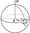 |
Fig. 1. Sketch of the local Cartesian model of the stellar convection zone. The local f-plane box is located at the equator, where the x, y, and z axes point to the longitudinal, latitudinal, and radial directions, respectively. |
2.2. Background stratification and radiative heating
The time-independent background quantities ρ0, p0, and T0 are given by an adiabatically stratified polytrope as (e.g., Fan et al. 1999)
![Mathematical equation: $$ \begin{aligned} \rho _{0}(z)&=\rho _{\mathrm{r} }\left[1-\frac{z}{(1+m)H_{\mathrm{r} }} \right]^{m}, \end{aligned} $$](/articles/aa/full_html/2025/11/aa56923-25/aa56923-25-eq6.gif) (6)
(6)
![Mathematical equation: $$ \begin{aligned} p_{0}(z)&=p_{\mathrm{r} }\left[1-\frac{z}{(1+m)H_{\mathrm{r} }} \right]^{1+m}, \end{aligned} $$](/articles/aa/full_html/2025/11/aa56923-25/aa56923-25-eq7.gif) (7)
(7)
![Mathematical equation: $$ \begin{aligned} T_{0}(z)&=T_{\mathrm{r} }\left[1-\frac{z}{(1+m)H_{\mathrm{r} }} \right], \end{aligned} $$](/articles/aa/full_html/2025/11/aa56923-25/aa56923-25-eq8.gif) (8)
(8)
 (9)
(9)
where m = 1/(γ − 1) is a polytropic index and ρr, pr, Tr, and Hr denote the values of ρ0, p0, T0, and the pressure scale height, H0, at the bottom of our numerical domain, z = 0.
In our model, the convective instability is driven by a prescribed radiative heating and cooling term through which the radiative energy flux is injected from the bottom boundary and extracted through the upper boundary:
![Mathematical equation: $$ \begin{aligned} Q_{\mathrm{rad} }(z) = -\frac{\partial }{\partial z} [ F_{\mathrm{heat} }(z)+F_{\mathrm{cool} }(z) ]. \end{aligned} $$](/articles/aa/full_html/2025/11/aa56923-25/aa56923-25-eq10.gif) (10)
(10)
We use the same functional forms for Fheat(z) and Fcool(z) as those presented in Bekki et al. (2017). The radiative heating part is assumed to be proportional to the background pressure as (Featherstone & Hindman 2016)
![Mathematical equation: $$ \begin{aligned} -\frac{\partial F_{\mathrm{heat} }}{\partial z}= f_{\mathrm{heat} } [p_{0}(z)-p_{0}(z_{\mathrm{max} })], \end{aligned} $$](/articles/aa/full_html/2025/11/aa56923-25/aa56923-25-eq11.gif) (11)
(11)
where the normalization factor, fheat, is determined by the input energy flux, F*, as
![Mathematical equation: $$ \begin{aligned} f_{\mathrm{heat} }=F_{*}\left[\int _{0}^{z_{\mathrm{max} }} (p_{0}(z)-p_{0}(z_{\mathrm{max} })) dz \right]^{-1}. \end{aligned} $$](/articles/aa/full_html/2025/11/aa56923-25/aa56923-25-eq12.gif) (12)
(12)
The radiative cooling flux, Fcool, is assumed to be a Gaussian function localized near the surface
![Mathematical equation: $$ \begin{aligned} F_{\mathrm{cool} }= F_{*} \exp {\left[ -\left(\frac{z-z_{\mathrm{max} }}{d_{\mathrm{cool} }} \right)^{2}\right]}, \end{aligned} $$](/articles/aa/full_html/2025/11/aa56923-25/aa56923-25-eq13.gif) (13)
(13)
where the thickness of the surface cooling layer is set to be dcool = 0.3 Hr, which is roughly the local pressure scale height at the top boundary.
2.3. Dimensionless parameters
The typical convective velocity, v*, is estimated as
 (14)
(14)
The typical convective turnover timescale, τ*, and the typical magnetic field strength, B*, are then estimated, respectively, as
 (15)
(15)
In our model, the radiative energy flux, F*, is set by specifying the modified Mach number, M* (square root of the Euler number),
 (16)
(16)
Although M* is estimated to be ≈𝒪(10−3 − 10−4) in the Sun’s convection zone (Ossendrijver 2003), we use the value of M* = 10−2 throughout this paper in order to avoid the severe CFL condition, while keeping thermal convection sufficiently subsonic. The rotational influence on convection is controlled by
 (17)
(17)
which we vary as a free input parameter from 1 to 20 as shown in Table 1. We note that the parameter Co* is defined a priori on measurable quantities of the Sun (such as the luminosity, L⊙, and rotation rate, Ω⊙) and is called a flux Coriolis number (e.g., Aurnou et al. 2020; Käpylä 2024). For reference, the solar value of Co* is estimated to be Co⊙ ≈ 3.8 (with F⊙ = 1.2 × 10¹¹ g s−3, Ω⊙ = 2.8 × 10⁻⁶ s−1, Hr = 57 Mm, and ρr = 0.2 g cm−3).
Summary of the numerical simulations reported in this paper.
2.4. Numerical methods
We numerically solved Eqs. (1)–(4) using the fourth-order central-differencing method and four-step Runge-Kutta scheme (e.g., Vögler et al. 2005). In order to keep the divergence-free condition of the magnetic field, the nine-wave method is used (Dedner et al. 2002). In this study, we do not use any explicit diffusivities but only use the slope-limited artificial diffusion proposed by Rempel (2014) to stabilize the computations (see Appendix A for details). The kinetic and magnetic energy dissipated through this artificial diffusion is returned to the internal energy. We note that this approach leads to effective thermal and magnetic Prandtl numbers in our simulations of order unity, both of which are much higher than those estimated in the real Sun.
The size of the numerical domain is (Lx, Ly, Lz)/Hr = (19.8, 6.6, 2.2), which is sufficiently large in the longitudinal (x) direction to capture the columnar convective pattern. The density contrast between the bottom and top of the numerical domain is about 24, with the number of density scale heights Nρ ≈ 3.2. We use a periodic boundary condition for horizontal directions and an impenetrable, stress-free boundary condition at the vertical boundaries. The magnetic field is assumed to be horizontal at the bottom (z = 0) and vertical at the top boundary (z = Lz). For all our simulations, we use the grid resolution of (Nx, Ny, Nz) = (1560, 520, 192). Owing to the nature of our diffusion scheme, this resolution determines the effective viscous, thermal, and magnetic diffusivities in the simulations. Each simulation was initiated by giving a small random perturbation to the vertical velocity, vz, while setting the other hydrodynamic (HD) variables ρ1, vx, vy, and s1 to zero. A weak seed field of (Bx, By, Bz)/B* = (0, 10−5, 0) was imposed to initiate the SSD at t = 0 in the MHD cases.
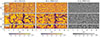 |
Fig. 4. Same as Fig. 3 but from the simulation cases HD-Co2 and MHD-Co2. An animation of this figure is available online. |
3. Results
3.1. Simulation overview
As is summarized in Table 1, we carried out sets of nonmagnetic (denoted by “HD”) and magnetic (denoted by “MHD”) simulations with five different rotational influences (Co* = 1, 2, 5, 10, 20). It is generally known that increasing Co* leads to a reduction in the supercriticality of convection (e.g., Chandrasekhar 1961). Exploring the effects of varying supercriticality requires huge numerical resources and is thus beyond the scope of this paper. Since the f-plane box is located exactly at the equator, the mean flow is only established in the x (longitudinal) direction. Furthermore, we note that our MHD simulations show no clear evidence of large-scale dynamo action.
Figure 2 shows the temporal evolution of the volume-integrated kinetic and magnetic energies, Ekin and Emag, from the MHD cases. They are defined by
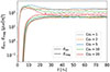 |
Fig. 2. Temporal evolution of the volume-integrated kinetic and magnetic energies, Ekin (dashed curves) and Emag (solid curves), from the MHD runs. Different colors represent the results with different Co*. |
 (18)
(18)
 (19)
(19)
where V = LxLyLz is the total volume of the numerical domain. All our simulations operate in a highly turbulent regime with effective Reynolds and magnetic Reynolds numbers, Re*, Rm* ≈ 103 (see Appendix A for details), which are sufficiently large to ensure vigorous convection and efficient SSD action. All the simulations were run for about 80 τ*. The SSDs are saturated and the statistically stationary states are reached by t ≈ 20 τ*. In what follows, we focus on these statistically stationary states.
Figure 3 shows the overall spatial patterns of the vertical velocity, vz, and vertical magnetic field, Bz, in the HD-Co1 and MHD-Co1 cases in which the rotational influence is weak (Co* = 1). In the MHD case (Fig. 3c), the results are very similar to those of nonrotating SSD simulations (Cattaneo 1999; Vögler et al. 2005; Rempel 2014; Hotta et al. 2015b). Strong mixed-polarity magnetic fields are predominantly concentrated in the narrow downflow regions that are surrounded by slower and broader upflows. A comparison of the HD and MHD cases (Figs. 3a and b) also reveals that the convective pattern in MHD becomes much smoother than that of HD simulation. This can be attributed to the back-reaction from the SSD, i.e., the small-scale Lorentz force suppresses the small-scale turbulence (Hotta et al. 2015b).
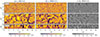 |
Fig. 3. Temporal snapshots of (a) the vertical velocity, vz, from case HD-Co1, (b) vz from case MHD-Co1, and (c) the vertical magnetic field, Bz, from MHD-Co1 in the statistically stationary states at t ≈ 80 τ*. The top and middle panels show the horizontal cuts near the top surface, z = 2.2 Hr, and in the middle convection zone, z = 1.2 Hr. The bottom panels show the vertical cuts at y = 0. An animation of this figure is available online. |
Figures 4, 5, 6, and 7 show the temporal snapshots of vz and Bz in the same way as in Fig. 3 but with increasing Co*. As Co* increases, the columnar pattern elongated in the y direction becomes more and more apparent. The size (longitudinal extent) of the convective columns becomes smaller with the increase in Co*. In other words, the total number of columns in the x direction increases as convection becomes more and more rotationally constrained. Furthermore, a comparison between the HD and MHD cases again shows that the columnar pattern tends to be much more coherent and self-organized in the magnetized convection (e.g., Figs. 7a and b).
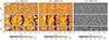 |
Fig. 5. Same as Fig. 3 but from the simulation cases HD-Co5 and MHD-Co5. An animation of this figure is available online. |
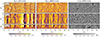 |
Fig. 6. Same as Fig. 3 but from the simulation cases HD-Co10 and MHD-Co10. An animation of this figure is available online. |
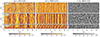 |
Fig. 7. Same as Fig. 3 but from the simulation cases HD-Co20 and MHD-Co20. An animation of this figure is available online. |
3.2. Notation of averages, Fourier spectra, and error estimates in this paper
In the following sections, we discuss several statistical properties of rotating magneto-convection. To this end, we define the following averaging procedures. The horizontal (x and y) average ⟨q⟩, the vertical (z) average  , and the latitudinal (y) average
  of a quantity, q, are defined as
 (20)
(20)
 (21)
(21)
 (22)
(22)
Fluctuations with respect to the horizontally averaged values are quoted by primes as
 (23)
(23)
In addition to this, we explicitly denote the fluctuations with respect to the y-averaged quantities by y primes as
 (24)
(24)
We also define a Fourier transform in the horizontal directions as
 (25)
(25)
where kx and ky are wavenumbers in the x and y directions. We note that discretized wavenumbers (kx, ky) = (2πnx/Lx, 2πny/Ly) with integers nx, ny (≥0) are used.
Hereafter, we discuss the statistical properties averaged over time between 60 ≤ t/τ* ≤ 80, with the standard errors given by  , where σ denotes the standard deviation and Nt is the number of temporal snapshots used. To ensure that the snapshots are statistically independent, we used the data at intervals of 1.0 τ*, i.e., Nt = 20.
3.3. Energy spectra
Figure 8 exemplifies the 2D kinetic energy spectra in the middle convection zone (z = 1.1 Hr) for weak rotation (Co* = 1) and strong rotation (Co* = 20) cases. Here, the kinetic energy spectrum,  , is defined as
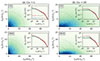 |
Fig. 8. Two-dimensional kinetic energy spectra shown in a horizontal wavenumber space (kx, ky) in the middle convection zone (z = 1.1 Hr) for (a) weakly rotating and (b) rapidly rotating cases. The top and bottom rows show the results of HD and MHD simulations, respectively. The insets show cuts of the same spectra at fixed ky, where the red, blue, green, and gray curves correspond to cuts through kyLy/2π = 0, 1, 2, and 3. |
 (26)
(26)
By definition, this satisfies
 (27)
(27)
Although the distribution of convective power in wavenumber space (kx, ky) is almost isotropic in Co* = 1 cases, the spectra become strongly anisotropic in Co* = 20 cases wherein most power is concentrated in the Fourier domain where the latitudinal wavenumber, ky, is small. In fact, as is indicated by the inset panels in Fig. 8b, the ky = 0 component of the convective motions is shown to be dominant over the ky ≠ 0 components. This corresponds to a formation of coherent columnar patterns aligned in the y direction (Figs. 6 and 7).
Figures 9a and b show the kinetic energy spectra summed over ky for HD and MHD cases for different values of Co*. When Co* is small, the kinetic energy spectra roughly follow the Kolmogorov power law  in the inertial spectral range. However, when Co* is increased,
  begins to show spectral peaks at higher longitudinal wavenumbers. In MHD simulations, we also show the magnetic energy spectra,
  , defined by
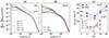 |
Fig. 9. (a) Kinetic energy spectra, |


 (28)
(28)
We find that the SSD generates super-equipartition (i.e.,  ) magnetic fields at small scales. Consequently, the kinetic energy,
  , is suppressed due to the Lorentz force feedback at these scales.
It is important to note that, in our simulations, there are two distinct characteristic length scales. One is the mean longitudinal wavenumber, kx, mean, weighted by the kinetic energy spectrum (e.g., Christensen & Aubert 2006; Käpylä 2024),
 (29)
(29)
and the other is the peak longitudinal wavenumber, kx, peak, at which the kinetic energy spectrum reaches its maximum. In previous studies of rotating f-plane simulations in which gravity is aligned with the rotation axis, these two wavenumbers become asymptotically equivalent in the rapidly rotating limit (e.g., Käpylä 2024). However, in our model setup, in which both small-scale convective motions and large-scale columnar convective modes coexist, they do not coincide. Figure 9c shows the height-averaged mean wavenumber,  , and the peak wavenumber,
  , as functions of Co*. In general, the inclusion of the SSD leads to smaller
  in MHD (i.e., the typical convective scale
  becomes larger) than in HD because the SSD Lorentz force suppresses small-scale turbulence. In contrast, the peak wavenumber,
  , is shown to be systematically larger in MHD at Co* ≥ 5. We find that the peak wavenumber,
  , largely represents the dominant scale of the ky = 0 columnar convective (thermal Rossby) modes. The effects of the SSD on
  are discussed later in Sect. 3.6.
3.4. Convective heat transport
Figures 10a–d show vertical profiles of the root-mean-square (rms) convective velocity
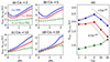 |
Fig. 10. Profiles of the rms convective velocity, vrms, and the Alfvén velocity of the rms magnetic field, |


 (30)
(30)
where Ux = ⟨vx⟩ denotes the mean flow in the x direction. The generation mechanisms of the mean flows are discussed in a later section (Sect. 3.7). From MHD simulations, we also show the Alfvén velocity associated with the rms magnetic field,
 (31)
(31)
It is evident that, due to the SSD Lorentz force feedback, vrms in the MHD cases is suppressed by approximately 15–25% compared to the HD cases. In most of our simulations, the rms field strength, Brms, is sub-equipartition, i.e., vA, rms < vrms. Although this is in accordance with the simulations by Favier & Bushby (2012) and Warnecke et al. (2025), we note that the higher-resolution simulation by Hotta et al. (2022) produces super-equipartition SSD fields throughout the whole convection zone.
It is generally known that strong rotation tends to suppress convective velocities (e.g., Aurnou et al. 2020; Vasil et al. 2021; Käpylä 2024). As is shown in Fig. 10e, our simulations also demonstrate that the volume-averaged rms convective velocity,  , decreases with increasing Co* in the rapidly rotating regime (Co* ≥ 5) in both HD and MHD cases. Moreover, our study reveals that this suppression is further enhanced by the presence of SSD. In HD,
  decreases gradually with Co*, roughly following a power law of Co*−1/5, while in MHD, the decline is steeper, following Co*−1/3, as indicated by the dotted gray lines in Fig. 10e. The underlying mechanism by which the SSD modifies the Co* dependence is explained in Sect. 3.5.
Next, we discuss thermal energy transport properties in our simulations. Figures 11a–d present snapshots of the entropy perturbations,  , for Co* = 2 and 20. Figure 11e further shows the vertically averaged rms entropy perturbations,
  , as a function of Co*. Here, srms is defined by
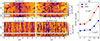 |
Fig. 11. Entropy perturbations, s′1, in our simulations. (a,b) Temporal snapshots of s′1 weighted by the background density, ρ0, at fixed height (z = 1.2 Hr) and latitude (y = 0) from weakly rotating simulations HD-Co2 and MHD-Co2. (c,d) Same as panels a and b but from rapidly rotating cases HD-Co20 and MHD-Co20. (e) Volume-averaged rms entropy perturbation, |


 (32)
(32)
We note that the entropy perturbations shown are weighted by the background density, ρ0, which allows us to focus on the entropy variations within the bulk convection zone, rather than those generated by strong near-surface radiative cooling. Two main effects are observed. First, we find an enhancement of the entropy perturbations, s′1, due to the SSD action. This behavior was reported in earlier nonrotating studies (e.g., Hotta et al. 2015b), in which it was shown that the SSD magnetic fields suppress horizontal turbulent mixing of entropy between warm upflows and cold downflows, thereby enhancing entropy contrast. At small Co*, the MHD simulations show an increase in srms by approximately 25% compared to the HD cases. The second effect is an enhancement of s′1 by strong rotation at Co* ≥ 5. It is well known that the Coriolis force makes the convective heat transport inefficient as it deflects vertical motions and reduces the entropy mixing in a vertical direction. To sustain a fixed enthalpy flux in the domain, the entropy perturbations, s′1, are enhanced. As is shown in Fig. 11e, the volume-averaged rms entropy perturbation,  , increases with Co* in both the HD and MHD cases. However, the scaling differs: the MHD cases follow an approximate scaling of Co*1/3, while the HD cases follow Co*1/5, indicating a stronger Co* dependence with the presence of SSD. Obviously, these scalings are the inverse of those found in the rms convective velocity, vrms (Fig. 10e), implying that the entropy perturbations are enhanced to compensate for the reduced convective velocities and to transport the fixed amount of enthalpy upward.
The efficiency of convective energy transport is known to be associated with the mean entropy stratification in the bulk convection zone. Figures 12a–d show vertical profiles of the superadiabaticity, δ, defined as
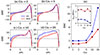 |
Fig. 12. Profiles of the superadiabaticity, δ. (a–d) Vertical profiles of δ for different Co*. Blue and red curves represent the results from HD and MHD simulations. (e) Volume-averaged values of superadiabaticity, |

 (33)
(33)
When the rotational influence is weak, a weakly subadiabatic layer is formed in the lower half of the convection zone. This is because of the nonlocal heat transport by strong downflow plumes (e.g., Brandenburg 2016) and has been repeatedly reported in previous simulations of nonrotating convection (e.g., Käpylä et al. 2017b; Bekki et al. 2017; Karak et al. 2018; Käpylä 2025). It is also seen that the magnitude and width of this subadiabatic layer are enhanced and extended with the inclusion of SSD. When Co* is increased, the mean stratification becomes more superadiabatic in the bulk convection zone because the rotation suppresses vertical entropy mixing. These trends are clearly seen in Fig. 12e. Interestingly, we find that the SSD makes the subadiabatic layer near the base of the convection zone persistent even under strong rotational influence (see the inset of Fig. 12e). This result is in striking contrast to the HD case in which the subadiabatic layer vanishes in the rapidly rotating regime. A disappearance of the subadiabatic layer in the rapidly rotating HD regime has also been reported by Käpylä (2024), who employed a radiative diffusivity based on Kramers opacity (as a function of temperature and density) instead of the spatially fixed radiative heating used in this study.
Our parameter study suggests that the weakly subadiabatic layer likely exists in the lower 40% of the Sun’s convection zone near the equator (given that Co⊙ ≈ 3.8). A similar result is obtained by Hotta et al. (2022). We also note that the existence of this weakly subadiabatic layer in the Sun’s convection zone has been inferred by recent observations and linear modeling of the non-toroidal class of the solar inertial modes (Hanson et al. 2022; Bekki 2024).
3.5. Force balance
To understand why the convective velocity, vrms, and entropy fluctuation, srms, show different Co* dependences with and without the SSD, we investigate the dominant force balance in our simulations. We follow the method presented in Yadav et al. (2016), Aguirre Guzmán et al. (2021) and compute the rms values of the following forces:
 (34)
(34)
 (35)
(35)
 (36)
(36)
 (37)
(37)
 (38)
(38)
Here, we note that temporally averaged component of the pressure and buoyancy forces (which represents the background hydrostatic balance and thus is irrelevant to our analysis) are subtracted from FPre and FBuo. Figure 13a shows the rms forces in HD (top) and MHD (bottom) cases as functions of Co*. In HD simulations, the advection (or inertia) term FAdv always dominates the force balance. As Co* is increased, a balance is achieved among advection, FAdv, pressure, FPre, and Coriolis forces, FCor. On the other hand, in MHD simulations, the Lorentz force, FMag, comes into play in the leading-order force balance, where FMag has amplitudes very close to those of the pressure gradient force, FPre. This likely reflects the fact that the strong SSD fields are generated by compression of downflows where the gas pressure is locally balanced by the magnetic pressure (Hotta et al. 2022). At sufficiently high Co*, FMag is even stronger than FAdv, leading to a balance between the pressure, FPre, Coriolis, FCor, and Lorentz forces, FMag. This balance is called magnetostrophic (e.g., Roberts 1978). We can attribute the Co* dependences of vrms and srms discussed in Sect. 3.4 to this transition of the dominant force balance regime.
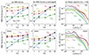 |
Fig. 13. Force balances in our simulations. (a) RMS amplitudes of the forces, Frms. Here, Frms is calculated such that Frms2 = V−1∫V(Fx′2 + Fy′2 + Fz′2)dV. Yellow, red, green, blue, and purple colors represent the nonlinear advection, pressure gradient, buoyancy, Coriolis, and Lorentz forces. The top and bottom panels show the HD and MHD simulations, respectively. (b) RMS amplitudes of the y-averaged forces, |


It is worth noting that the relative importance of the Coriolis force, FCor (which does not have a y component), tends to be underestimated in Fig. 13a. To properly assess the significance of the Coriolis force in the system, we also compute the same rms forces but for the y-averaged ones, as shown in Fig. 13b. We can see that there is a clear distinction between the weakly rotating regime, Co* < 5, where the Coriolis force,  , is not in the leading-order force balance and the strongly rotating regime, Co* ≳ 5, where the dominant force balance is achieved between the Coriolis force,
  , and the pressure gradient force,
  . When this geostrophic balance is established at a leading order, it is necessary to look at the residual balance (e.g., Yadav et al. 2016; Aubert et al. 2017). Figure 13c displays the power spectra of the y-averaged forces in the middle convection zone (z = 1.1 Hr) from rapidly rotating HD-Co20 and MHD-Co20 cases. Here, the imbalance between Coriolis and pressure gradient forces,
  , is denoted by dashed gray curves. In the HD case, this so-called ageostrophic Coriolis force is balanced by buoyancy,
  , and advection,
  , at large scales and predominantly by advection at small scales, manifesting the Coriolis-Inertia-Archimedean (CIA) balance (see, e.g., Aurnou et al. 2020; Käpylä 2024). In the MHD case, on the other hand, the ageostrophic Coriolis force is primarily balanced by buoyancy,
  , at large scales but is balanced by the Lorentz force,
  , at small scales, manifesting the magneto-Archimedean-Coriolis (MAC) balance (see, e.g., Davidson 2013; Augustson et al. 2019; Schwaiger et al. 2021).
Assuming the CIA and MAC balances, the following scaling relations can be derived in terms of the flux Coriolis number, Co* (see Appendix B for detailed derivations):
 (39)
(39)
 (40)
(40)
 (41)
(41)
In Figs. 9c, 10e, and 11e, our simulated Co* dependences are compared with these theoretical scalings. It is clearly seen that our results are consistent with the predictions by CIA and MAC balances at Co* ≥ 5.
One might question the robustness of the above results, particularly when the numerical resolution is further increased. Hints are provided by Käpylä (2024), who conducted HD simulations at varying Reynolds number Re and demonstrated that the scaling of convective velocity, vrms, with Coriolis number remains unaffected, although the overall amplitude of vrms increases with Re. This is because viscous force does not influence the dominant force balance. Given that the CIA and MAC balances are well established in our simulations, the above scaling relations at the high-Co* regime are expected to remain robust even at higher resolutions, although the absolute values of vrms (or srms) and the degree of suppression (enhancement) from HD to MHD will be affected.
3.6. Dominant scale of columnar convection
In this subsection, we discuss how SSD affects the dominant scale of columnar convective modes. From Figs. 7a and b, it is seen that the SSD not only makes the columnar patterns more self-organized but also shifts the dominant longitudinal scale of convection narrower. To quantify the difference in the length scales of columnar convection, we compare in Fig. 14a the kinetic energy spectra between HD and MHD cases in the middle convection zone (z = 1.1 Hr). Figure 14b shows the peak longitudinal wavenumber,  , as a function of Co*. In both the HD and MHD cases, there is a general trend that
  increases with Co*. However, it is obvious that the MHD simulations show a much more rapid increase in
  with Co* compared to the HD counterparts. As a consequence, in the high-Co* regime, the convective columns have a smaller length scale in longitude with the presence of the SSD. This behavior cannot be explained by the CIA/MAC scaling relations (Eq. 39).
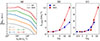 |
Fig. 14. (a) Normalized kinetic energy spectra, |


We find that, through the suppression in the convective velocity, vrms, and the increase in the (mean) convective length scale, ℓx = 2π/kx, mean, the SSD can change the effective rotational influence in the simulations. This is typically measured by the dynamical Coriolis number,
 (42)
(42)
As is reported in Table 1, Coℓ is systematically larger in MHD than in HD, implying that the MHD simulations are operating in more rotationally constrained regimes compared to the HD counterparts. Consequently, the establishment of the columnar patterns is more enhanced and the longitudinal size of these columns becomes smaller in our MHD simulations. In fact, we find that the peak wavenumbers,  , in both the HD and MHD cases manifest very similar dependences on the dynamical Coriolis number, Coℓ (Fig. 14c). This provides supporting evidence that the dominant scale of columnar convection is largely determined by Coℓ, a parameter that is sensitively affected by the SSD.
We also note that there are other underlying mechanisms that can potentially explain the difference in  between HD and MHD. The first possibility is direct Lorentz force feedback. As is shown in Sect. 3.8, the large-scale shear motions in the columnar convection can generate the Maxwell stress to redistribute the angular momentum in the convection zone. As a back-reaction, the kinetic energy of columnar convection is suppressed at large scales, which can also cause a shift in
  toward higher wavenumbers. Another possible mechanism comes through the change in the mean background stratification. When the SSD is present, the buoyant driving can be selectively suppressed at large scales due to the reduced superadiabaticity and the existence of the weakly subadiabatic layer near the base of the convection zone (Fig. 12). Yet, it is not easy to disentangle these mechanisms and to pinpoint the primary cause. Such an analysis is beyond the scope of this paper.
3.7. Mean flow generation
In our simulations, large-scale mean flows are generated only in the longitudinal direction, Ux(z) = ⟨vx⟩, corresponding to the radial differential rotation at the equator. Figures 15a–d show profiles of Ux(z) established in our HD and MHD simulations for different values of Co*. A mean flow regime can be measured by the vertical shear, ΔUx = Ux(zmax)−Ux(zmin), as is shown in Fig. 15e. For Co* = 1, 2, and 5, the mean flows have negative vertical shear, ΔUx < 0, with a faster base and a slower surface. This might correspond to an antisolar differential rotation profile in a spherical shell geometry. On the other hand, for Co* = 10 and 20, the mean flows show a positive vertical shear, ΔUx > 0, with a faster surface and a slower base, likely corresponding to a solar-like rotational profile in the spherical case. We find that the inclusion of the SSD has the primary impact of quenching the mean flow amplitudes at high Co*, as has been reported in the literature (e.g., Brun et al. 2004; Käpylä et al. 2017a; Matilsky et al. 2022; Warnecke et al. 2025).
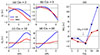 |
Fig. 15. Profiles of the mean flows, Ux(z). (a–d) Vertical profiles of Ux(z) for different Co*. Blue and red colors represent the results from the HD and MHD simulations. (e) Vertical shear amplitudes of the mean flow, ΔUx = Ux(zmax)−Ux(zmin), as a function of Co*. |
Another important effect of the SSD on the mean flow, Ux, is the excitation of torsional oscillations, i.e., temporal variations in the mean flow. In our model, these oscillations arise as a by-product of the establishment of the MAC balance, whereby torsional Alfvén waves propagate vertically as disturbances to the so-called Taylor state (Taylor 1963; Braginskiy 1970; Wicht & Christensen 2010). Our analysis indicates that their amplitudes are too small (a few percent of the rms velocity fluctuation) to have a dynamical impact in the simulation. Therefore, a more detailed discussion is deferred to the Appendix C.
We now discuss the generation mechanism of the mean flows. Taking a horizontal average of the x component of Eq. (2), we have
 (43)
(43)
where
 (44)
(44)
are the turbulent Reynolds and Maxwell stresses, respectively. Positive and negative values of ℛxz and ℳxz correspond to vertically upward and downward fluxes of the x (angular) momentum. Figures 16a–d show vertical profiles of ℛxz and ℳxz for different Co*. Their height-averaged values are shown as functions of Co* in Fig. 16e. Note that, in HD, ℛxz must vanish in a statistically stationary state (∂Ux/∂t ≈ 0). This reflects a balance between the diffusive and non-diffusive (the Λ effect) parts of the Reynolds stress, ℛxz, which transport angular momentum in opposite directions (Kitchatinov 2013; Barekat et al. 2021). In MHD, ℛxz and ℳxz must balance with each other such that their sum vanishes statistically. At low Co* (≤5) where the mean flow is antisolar (ΔUx < 0), the Reynolds stress is negative ( , and the Maxwell stress is positive (
 ). Conversely, at high Co* (≥10) where the mean flow is solar-like (ΔUx > 0), the signs of the Reynolds and Maxwell stresses are flipped;
  and
and  . Thus, we conclude that the mean flows are primarily generated by the angular momentum transport (AMT) through the Reynolds stress, ℛxz, with the Maxwell stress, ℳxz, only playing a suppressive role. At low Co*, the antisolar mean flows are established by the downward AMT by weakly rotationally constrained convection (Foukal & Jokipii 1975; Guerrero et al. 2013; Featherstone & Miesch 2015), whereas at high Co*, the upward AMT by rotationally constrained convective columns leads to the solar-like mean flows (Hotta et al. 2015a; Matilsky et al. 2019; Bekki et al. 2022b) (see also Appendix D for a schematic explanation).
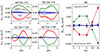 |
Fig. 16. Profiles of the Reynolds and Maxwell stresses, defined by Eq. (44). Positive and negative values correspond to the upward and downward AMT. (a–d) Vertical profiles of the Reynolds stress, ℛxz, for different values of Co*. Blue and red colors represent the results from the HD and MHD cases. Green curves show the vertical profiles of the Maxwell stress, ℳxz, and the dashed black curves indicate the sum ℛxz + ℳxz in the MHD simulations. (e) Volume-averaged Reynolds and Maxwell stresses, |


To assess the impact of the columnar convective modes on AMT, we decompose the Reynolds stress into contributions from the y-averaged flows (representing the ky = 0 columnar modes), ℛxzky = 0, and those from the velocity fluctuations, ℛxzky ≠ 0, as
 (45)
(45)
Figures 17a and b show the volume-averaged Reynolds stress contributions,  and
and  . There is a general tendency for the ky = 0 columnar modes to transport angular momentum upward (
 ) and the small-scale fluctuating velocities transport angular momentum downward (
 ). In HD cases, these two contributions cancel each other. In particular, at high Co*,
  corresponds to a driving of the mean flow, ΔUx > 0, and
  corresponds to a turbulent diffusion. These tendencies are consistent with scale-by-scale analyses by Mori & Hotta (2023) and Käpylä (2023), who found downward AMT from small-scale turbulence and upward AMT from large-scale columnar modes near the equator. We note, however, that their analyses are based on longitudinal scale decompositions, whereas we distinguish the ky = 0 columnar modes from the ky ≠ 0 fluctuations; therefore, a one-to-one correspondence should not be assumed. In MHD cases, the cancellation between
  and
and  breaks down. At low Co*, the ky ≠ 0 convective motions that are weakly influenced by rotation dominantly transport angular momentum downward. As Co* increases, the rotationally constrained columnar modes become increasingly dominant, resulting in net upward AMT (see Appendix D). Here, the downward AMT by ky ≠ 0 flows is substantially reduced because the effective eddy diffusion due to small-scale turbulence is suppressed by the SSD Lorentz force. The resulting net downward (upward) angular momentum flux at low (high) Co* is then compensated for by the upward (downward) flux of the Maxwell stress, where all the contributions are from ky ≠ 0 magnetic fields (Fig. 17c).
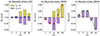 |
Fig. 17. Breakdown of the contributions from the ky = 0 and ky ≠ 0 components to the Reynolds and Maxwell stresses. (a,b) Volume-averaged Reynolds stress, |


3.8. Origin of Maxwell stress: Interplay with convective columns
In this subsection, we discuss the generation mechanisms of the Maxwell stress, ℳxz. To this end, we compare the spatial distribution of the magnetic field correlation  (averaged over y) with various y-averaged quantities, as is shown in Fig. 18. Let us first focus on the low-Co* regime in which the Maxwell stress transports angular momentum upward (
 ). It is seen from Figs. 18a and b that the magnetic field correlation,
  , is not necessarily generated in downflow regions where strong magnetic energy is concentrated and where the velocity correlation,
  , is dominantly generated. As a result, the spatial distribution of
  is poorly correlated with that of
  (Fig. 19a). This implies that the generation of the Maxwell stress is not a consequence of a parallelization of the small-scale magnetic fields with the small-scale flows, as has been proposed by Hotta et al. (2022). Rather, in our simulations, the spatial distribution of
  is very well correlated with those of the y vorticity,
  , and also of the pressure perturbation,
  . The latter is in fact a side effect required by the geostrophic balance (anticorrelation between
  and
and  ).
).
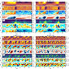 |
Fig. 18. Snapshots of the y-averaged quantities from MHD simulations with Co* = 2, 5, 10, and 20. Each panel, from top to bottom, displays the y-averaged profiles of the x velocity, |


A good correlation between the spatial distributions of  and
and  suggests that the shear in the columnar convection is the main origin of the Maxwell stress in our simulations. From the induction Eq. (3), we obtain
![Mathematical equation: $$ \begin{aligned} \frac{\partial }{\partial t} \widetilde{B_x B_z} = [\ldots ] + \widetilde{B_x^2} \frac{\partial \widetilde{v}^{\prime }_z}{\partial x} + \widetilde{B_z^2} \frac{\partial \widetilde{v}^{\prime }_x}{\partial z}, \end{aligned} $$](/articles/aa/full_html/2025/11/aa56923-25/aa56923-25-eq161.gif) (46)
(46)
indicating that  can be generated by shear motions in the y-averaged flows,
  and
and  . Therefore, if the main generation mechanism of the Maxwell stress is the columnar shear,
  must be strongly correlated with the velocity strain tensor,
  , defined as
 (47)
(47)
This is clearly shown to be the case from Figs. 19d–f. Since the longitudinal separation between columnar downflows is large at low Co*, the vertical shear of the zonal velocity dominates over the zonal shear of the vertical flow,  . In such a case, both
  and
and  are primarily determined by
  , which explains why
  and
and  are so well correlated in Fig. 18a and b. When averaged over the whole volume, the net correlation ⟨BxBz⟩ becomes negative because the y vorticity consists of spatially
  and broadened
  due to the nonlinear effect (see Appendix E for its physical explanation).
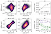 |
Fig. 19. (Top) Correlations between the Maxwell stress, |


Next, we discuss the results in the high-Co* regime (Figs. 18c and d). Under strong rotational influences, the longitudinal separation of the convective columns decreases and the zonal shear of the vertical flow becomes non-negligible. Consequently,  is no longer well correlated with
  . Instead,
  is now positively correlated with
  (Figs. 19b and c). This is not surprising because
  and
and  are both rooted in the y-coherent columnar pattern. We note, however, that this positive correlation between
  and
and  is not likely due to the local alignment of small-scale velocity to small-scale magnetic fields. As is clearly manifested by the strong correlation between
  and
and  in Fig. 19e, a main generation mechanism of a positive magnetic field correlation,
  , remains the shear motions in the columnar convection (both
  and
and  ). On the other hand, a positive velocity correlation,
  , is established as a consequence of the tilted pattern of the y-averaged columns (see Appendix D).
Our simulations clearly show that the Maxwell stress is primarily generated by the shear in the columnar motions, regardless of the rotational regime. This is in contrast to the results of Hotta et al. (2022), who argue that the Maxwell stress originates mainly from the Reynolds stress. One possible reason for this discrepancy lies in the differences in the simulation setups: their model covers a full spherical shell, in contrast to our equatorial local model, and the interaction between SSD and rotating convection at middle to high latitudes (where the columnar convection is absent) may play a dominant role. Moreover, in their simulations, the presence of super-equipartition magnetic fields can significantly suppress the velocity shear, which may inhibit the generation of Maxwell stress through shear.
3.9. Amplitudes of columnar modes
In all our simulations, we find that the velocity strain tensor,  , is not correlated with
  but is closely correlated with
  (Fig. 19f). This suggests that the Lorentz force associated with
  plays a significant role as an effective viscosity on the columnar convection, leading to a suppression of the columnar convective modes. Figure 20a shows the volume-integrated kinetic energy of the y-averaged flows,
 (48)
(48)
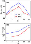 |
Fig. 20. Volume-integrated (a) kinetic energy, |


as a function of Co*. There is a general tendency seen in both HD and MHD cases that  first increases and then decreases as Co* increases. The initial increase in
  is simply due to the establishment of a coherent columnar pattern. The decrease in
  at Co* > 5 can be attributed to the suppression of convective velocity in a strongly rotationally constrained regime (Eq. 40). It would also be instructive to use the volume-integrated y enstrophy,
 (49)
(49)
as a measure of the amplitudes of the columnar modes. As shown in Fig. 20b,  increases monotonically with Co* in both the HD and MHD cases. Suppression of the columnar convection by the SSD can be seen in both
  and in
  . The suppression is the most drastic in the intermediate regime Co* = 5, in which both
  and
and  are reduced by about 40% from HD to MHD.
4. Summary and conclusions
In this paper, we have carried out a series of HD and MHD simulations of highly turbulent rotating compressible convection using a local f-plane box model at the equator. This model setup enabled us to focus on the effects of SSD on rotating columnar convection. We performed a parameter study in which the rotation rate was varied while the energy flux was fixed, covering the flux Coriolis number, Co*, from 1 to 20.
We find that the SSD has a significant impact on the properties of convective heat transport. As has been reported in previous nonrotating studies, the convective velocity, vrms, tends to be suppressed due to the Lorentz force feedback (Rempel 2014; Hotta et al. 2015b). Under strong rotational influences, we find that vrms decreases with Co* more rapidly in MHD cases than in their HD counterparts. That is, convection tends to be suppressed much more significantly by rotation when the SSD exists. This rapid decrease in vrms with Co* is compensated for by a rapid increase in the entropy fluctuations, srms, with increasing Co*, which is required for rotating convection to transport the fixed amount of enthalpy upward. One of the most striking outcomes of this entropy enhancement by the SSD is the existence of a weakly subadiabatic layer near the base of the convection zone, which persists even in a strongly rotationally constrained regime (Co* = 20). This is in significant contrast to rotating HD convection, in which the weakly subadiabatic layer vanishes when the rotational influence becomes strong enough (e.g., Käpylä 2024). The potential existence of this subadiabatic layer in rapidly rotating stars has profound implications for dynamo processes in young Sun-like stars (e.g., Brown et al. 2011; Viviani et al. 2018; Käpylä et al. 2019).
These results can be understood by investigating how SSD alters the dominant force balance. Our analysis reveals that, at small scales, the pressure gradient force is balanced by the Lorentz force rather than by inertia when the SSD is present, establishing the so-called magnetostrophic balance. On the other hand, at large scales, a geostrophic balance is always maintained. Consequently, the SSD causes a transformation of the regime of rotating convection from a quasi-geostrophic (QG) CIA balance to a QG MAC balance. In fact, it is shown that the Co* dependences of vrms and srms in our HD and MHD simulations are consistent with the theoretical scaling relations of the CIA and MAC balances in the rapidly rotating limit (Co* ≳ 5).
In rotating columnar convection, there are two distinct characteristic length scales. When a typical convective length scale is measured by a mean longitudinal wavenumber,  (weighted by the kinetic energy spectrum), we find that
  becomes smaller in MHD cases, i.e., the typical size of convective cells becomes larger, because the kinetic energy is suppressed at small scales due to the SSD Lorentz force feedback. In the rapidly rotating regime (Co* ≳ 5),
  increases with Co* in both HD and MHD cases, roughly consistent with the CIA and MAC scalings, respectively. On the other hand, the peak wavenumber,
  (at which the kinetic energy spectrum has a local maximum), represents the dominant scale of the prograde-propagating columnar convective (thermal Rossby) modes, and it does not follow the CIA and MAC scalings. Our analysis reveals that the SSD enhances the effective rotational influence on columnar convection by increasing the dynamical Coriolis number, Co
 . As a result, the dominant scale of columnar convection becomes smaller when the SSD is present.
In addition to the convective heat transport, we also find that the SSD has a significant impact on the convective AMT. As has already been reported in previous studies (e.g., Gastine et al. 2013; Guerrero et al. 2013; Mabuchi et al. 2015; Featherstone & Miesch 2015), we see a transition from the “antisolar” mean flow profile (with a faster base and a slower surface) to the “solar-like” mean flow profile (with a faster surface and a slower base) as Co* increases. We find that the SSD acts to suppress the amplitudes of the mean shear flows, as it provides a Maxwell stress that counteracts the Reynolds stress. This result is consistent with many previous studies (Brun et al. 2004; Nelson et al. 2013; Augustson et al. 2015; Käpylä et al. 2017a; Warnecke et al. 2025). Some spherical dynamo simulations (e.g., Fan & Fang 2014; Karak et al. 2015; Hotta et al. 2022; Soderlund et al. 2025) further reported that the magnetic field can change the rotational profile from antisolar to solar-like near the solar parameter regime (Co* ≈ 2 − 5). Such a drastic transition was not seen in this study. This can be primarily attributed to the lack of AMT via meridional circulation – an essential ingredient for the generation of differential rotation in spherical models – in our simplified f-plane box model.
In Hotta et al. (2022)’s simulation, a key to achieving solar-like differential rotation was the radially outward AMT by the SSD Maxwell stress. They proposed that this Maxwell stress arises as a back-reaction to the Reynolds stress because the small-scale magnetic fields tend to be parallel to the small-scale flows. In our simulations, we do not find clear evidence of this so-called punching-ball effect. In fact, we find that the y-averaged profile of the Maxwell stress,  , is poorly correlated with that of the Reynolds stress,
  , but is well correlated with those of the y vorticity,
  , or the vertical velocity shear,
  , of the columnar convection. This implies that the Maxwell stress in our simulations is mainly generated by the velocity shear associated with the large-scale convective columns, rather than by the Reynolds stress.
Our study highlights various impacts that SSD has on the properties of rotating columnar convection. These effects need to be taken into account to properly model rotating magneto-convection, particularly in rapidly rotating stars where SSD significantly alters the dominant force balance. Given that fully resolving SSD in global models of solar and stellar convection requires a substantial amount of computational resources, a promising alternative would be to develop subgrid-scale models that encapsulate the essential effects of SSD, as has been attempted in some earlier studies (Bekki et al. 2017; Hotta 2017; Karak et al. 2018).
In relation to the possible implications for the solar convective conundrum, one of the most striking issues is the absence of columnar patterns in the solar surface observations. In this work, we have shown that the SSD acts as an effective viscosity on columnar convection, contributing to the suppression of their mode power. In fact, the kinetic energy and enstrophy associated with columnar modes are reduced by approximately 30–50% due to the SSD effect (see Fig. 20). However, even in the presence of vigorous SSD, our simulations exhibit highly coherent columnar structures near the solar regime (Figs. 4–5). Therefore, the SSD effect alone is likely insufficient to fully account for the absence of observational evidence for columnar convection in the Sun. Some authors (e.g., Guerrero et al. 2013; Noraz et al. 2025) have suggested that the columnar patterns present in the deep convection zone may be obscured by small-scale granular convection near the surface. The density stratification in our simulations (Nρ ≈ 3.2) is not strong enough to produce such a concealing effect. Future investigations are required to determine how the results presented would change under conditions of stronger density stratification.
Data availability
Movies associated with Figs. 3–7 are available at https://www.aanda.org
Acknowledgments
The author appreciates an anonymous referee for the valuable remarks and suggestions. The author further thanks J. Wicht, T. Bhatia, and H. Hotta for their constructive comments. Y. B. acknowledges a support from ERC Synergy Grant WHOLESUN 810218. All the numerical computations were performed at GWDG and the Max-Planck supercomputer RZG in Garching. This work benefited from discussions within the NORDITA workshop “Stellar Convection: Modeling, Theory, and Observations”.
References
- Aguirre Guzmán, A. J., Madonia, M., Cheng, J. S., et al. 2021, J. Fluid. Mech., 928, A16 [Google Scholar]
- Aubert, J., Gastine, T., & Fournier, A. 2017, J. Fluid. Mech., 813, 558 [Google Scholar]
- Augustson, K., Brun, A. S., Miesch, M., & Toomre, J. 2015, ApJ, 809, 149 [Google Scholar]
- Augustson, K. C., Brun, A. S., & Toomre, J. 2019, ApJ, 876, 83 [Google Scholar]
- Aurnou, J. M., Horn, S., & Julien, K. 2020, Phys. Rev. Res., 2, 043115 [NASA ADS] [CrossRef] [Google Scholar]
- Barekat, A., Käpylä, M. J., Käpylä, P. J., Gilson, E. P., & Ji, H. 2021, A&A, 655, A79 [NASA ADS] [CrossRef] [EDP Sciences] [Google Scholar]
- Bekki, Y. 2024, A&A, 682, A39 [NASA ADS] [CrossRef] [EDP Sciences] [Google Scholar]
- Bekki, Y., Hotta, H., & Yokoyama, T. 2017, ApJ, 851, 74 [NASA ADS] [CrossRef] [Google Scholar]
- Bekki, Y., Cameron, R. H., & Gizon, L. 2022a, A&A, 662, A16 [NASA ADS] [CrossRef] [EDP Sciences] [Google Scholar]
- Bekki, Y., Cameron, R. H., & Gizon, L. 2022b, A&A, 666, A135 [NASA ADS] [CrossRef] [EDP Sciences] [Google Scholar]
- Bessolaz, N., & Brun, A. S. 2011, ApJ, 728, 115 [NASA ADS] [CrossRef] [Google Scholar]
- Bhatia, T. S., Cameron, R. H., Solanki, S. K., et al. 2022, A&A, 663, A166 [NASA ADS] [CrossRef] [EDP Sciences] [Google Scholar]
- Braginskiy, S. I. 1970, Geomagn. Aeron., 10, 1 [Google Scholar]
- Brandenburg, A. 2016, ApJ, 832, 6 [Google Scholar]
- Brown, B. P., Miesch, M. S., Browning, M. K., Brun, A. S., & Toomre, J. 2011, ApJ, 731, 69 [Google Scholar]
- Brun, A. S., & Toomre, J. 2002, ApJ, 570, 865 [CrossRef] [Google Scholar]
- Brun, A. S., Miesch, M. S., & Toomre, J. 2004, ApJ, 614, 1073 [Google Scholar]
- Brun, A. S., Strugarek, A., Noraz, Q., et al. 2022, ApJ, 926, 21 [NASA ADS] [CrossRef] [Google Scholar]
- Bushby, P. J., Käpylä, P. J., Masada, Y., et al. 2018, A&A, 612, A97 [NASA ADS] [CrossRef] [EDP Sciences] [Google Scholar]
- Busse, F. H. 1970, J. Fluid. Mech., 44, 441 [NASA ADS] [CrossRef] [Google Scholar]
- Busse, F. H. 2002, Phys. Fluids, 14, 1301 [NASA ADS] [CrossRef] [Google Scholar]
- Cattaneo, F. 1999, ApJ, 515, L39 [Google Scholar]
- Chandrasekhar, S. 1961, Hydrodynamic and Hydromagnetic Stability (Oxford: Clarendon) [Google Scholar]
- Christensen, U. R., & Aubert, J. 2006, Geophys. J. Int., 166, 97 [NASA ADS] [CrossRef] [Google Scholar]
- Davidson, P. A. 2013, Geophys. J. Int., 195, 67 [NASA ADS] [CrossRef] [Google Scholar]
- Dedner, A., Kemm, F., Kröner, D., et al. 2002, J. Comput. Phys., 175, 645 [Google Scholar]
- Evonuk, M. 2008, ApJ, 673, 1154 [NASA ADS] [CrossRef] [Google Scholar]
- Fan, Y., & Fang, F. 2014, ApJ, 789, 35 [NASA ADS] [CrossRef] [Google Scholar]
- Fan, Y., Zweibel, E. G., Linton, M. G., & Fisher, G. H. 1999, ApJ, 521, 460 [Google Scholar]
- Favier, B., & Bushby, P. J. 2012, J. Fluid. Mech., 690, 262 [Google Scholar]
- Featherstone, N. A., & Hindman, B. W. 2016, ApJ, 830, L15 [Google Scholar]
- Featherstone, N. A., & Miesch, M. S. 2015, ApJ, 804, 67 [Google Scholar]
- Foukal, P., & Jokipii, J. R. 1975, ApJ, 199, L71 [NASA ADS] [CrossRef] [Google Scholar]
- Gastine, T., Wicht, J., & Aurnou, J. M. 2013, Icarus, 225, 156 [Google Scholar]
- Gilman, P. A., & Miller, J. 1986, ApJS, 61, 585 [Google Scholar]
- Glatzmaier, G. A., & Gilman, P. A. 1981, ApJS, 45, 381 [NASA ADS] [CrossRef] [Google Scholar]
- Glatzmaier, G., Evonuk, M., & Rogers, T. 2009, Geophys. Astrophys. Fluid Dyn., 103, 31 [NASA ADS] [CrossRef] [Google Scholar]
- Guerrero, G., Smolarkiewicz, P. K., Kosovichev, A. G., & Mansour, N. N. 2013, ApJ, 779, 176 [NASA ADS] [CrossRef] [Google Scholar]
- Hanasoge, S. M., Duvall, T. L., & Sreenivasan, K. R. 2012, PNAS, 109, 11928 [NASA ADS] [CrossRef] [Google Scholar]
- Hanson, C. S., Hanasoge, S., & Sreenivasan, K. R. 2022, Nat. Astron., 6, 70 [Google Scholar]
- Hathaway, D. H., Teil, T., Norton, A. A., & Kitiashvili, I. 2015, ApJ, 811, 105 [Google Scholar]
- Hindman, B. W., & Jain, R. 2022, ApJ, 932, 68 [NASA ADS] [CrossRef] [Google Scholar]
- Hori, K., Jones, C. A., Antuñano, A., Fletcher, L. N., & Tobias, S. M. 2023, Nat. Astron., 7, 825 [Google Scholar]
- Hotta, H. 2017, ApJ, 845, 164 [Google Scholar]
- Hotta, H., Rempel, M., & Yokoyama, T. 2015a, ApJ, 798, 51 [Google Scholar]
- Hotta, H., Rempel, M., & Yokoyama, T. 2015b, ApJ, 803, 42 [NASA ADS] [CrossRef] [Google Scholar]
- Hotta, H., Rempel, M., & Yokoyama, T. 2016, Science, 351, 1427 [NASA ADS] [CrossRef] [Google Scholar]
- Hotta, H., Kusano, K., & Shimada, R. 2022, ApJ, 933, 199 [NASA ADS] [CrossRef] [Google Scholar]
- Hotta, H., Bekki, Y., Gizon, L., Noraz, Q., & Rast, M. 2023, Space Sci. Rev., 219, 77 [NASA ADS] [CrossRef] [Google Scholar]
- Howard, R., & Labonte, B. J. 1980, ApJ, 239, L33 [Google Scholar]
- Jain, R., & Hindman, B. W. 2023, ApJ, 958, 48 [Google Scholar]
- Käpylä, P. J. 2023, A&A, 669, A98 [NASA ADS] [CrossRef] [EDP Sciences] [Google Scholar]
- Käpylä, P. J. 2024, A&A, 683, A221 [NASA ADS] [CrossRef] [EDP Sciences] [Google Scholar]
- Käpylä, P. J. 2025, A&A, 698, L13 [NASA ADS] [CrossRef] [EDP Sciences] [Google Scholar]
- Käpylä, P. J., Korpi, M. J., & Brandenburg, A. 2009, ApJ, 697, 1153 [Google Scholar]
- Käpylä, P. J., Mantere, M. J., & Brandenburg, A. 2011, Astron. Nachr., 332, 883 [CrossRef] [Google Scholar]
- Käpylä, P. J., Käpylä, M. J., Olspert, N., Warnecke, J., & Brandenburg, A. 2017a, A&A, 599, A4 [NASA ADS] [CrossRef] [EDP Sciences] [Google Scholar]
- Käpylä, P. J., Rheinhardt, M., Brandenburg, A., et al. 2017b, ApJ, 845, L23 [CrossRef] [Google Scholar]
- Käpylä, P. J., Käpylä, M. J., & Brandenburg, A. 2018, Astron. Nachr., 339, 127 [CrossRef] [Google Scholar]
- Käpylä, P. J., Viviani, M., Käpylä, M. J., Brandenburg, A., & Spada, F. 2019, Geophys. Astrophys. Fluid Dyn., 113, 149 [CrossRef] [Google Scholar]
- Käpylä, P. J., Browning, M. K., Brun, A. S., Guerrero, G., & Warnecke, J. 2023, Space Sci. Rev., 219, 58 [CrossRef] [Google Scholar]
- Karak, B. B., Käpylä, P. J., Käpylä, M. J., et al. 2015, A&A, 576, A26 [NASA ADS] [CrossRef] [EDP Sciences] [Google Scholar]
- Karak, B. B., Miesch, M., & Bekki, Y. 2018, Phys. Fluids, 30, 046602 [NASA ADS] [CrossRef] [Google Scholar]
- Kitchatinov, L. L. 2013, IAU Symp., 294, 399 [Google Scholar]
- Mabuchi, J., Masada, Y., & Kageyama, A. 2015, ApJ, 806, 10 [NASA ADS] [CrossRef] [Google Scholar]
- Masada, Y., & Sano, T. 2014, PASJ, 66, S2 [Google Scholar]
- Matilsky, L. I., Hindman, B. W., & Toomre, J. 2019, ApJ, 871, 217 [NASA ADS] [CrossRef] [Google Scholar]
- Matilsky, L. I., Hindman, B. W., & Toomre, J. 2020, ApJ, 898, 111 [NASA ADS] [CrossRef] [Google Scholar]
- Matilsky, L. I., Hindman, B. W., Featherstone, N. A., Blume, C. C., & Toomre, J. 2022, ApJ, 940, L50 [NASA ADS] [CrossRef] [Google Scholar]
- Miesch, M. S. 2005, Liv. Rev. Sol. Phys., 2, 1 [Google Scholar]
- Miesch, M. S., Elliott, J. R., Toomre, J., et al. 2000, ApJ, 532, 593 [CrossRef] [Google Scholar]
- Miesch, M. S., Brun, A. S., DeRosa, M. L., & Toomre, J. 2008, ApJ, 673, 557 [NASA ADS] [CrossRef] [Google Scholar]
- Mori, K., & Hotta, H. 2023, MNRAS, 519, 3091 [Google Scholar]
- Nelson, N. J., Brown, B. P., Brun, A. S., Miesch, M. S., & Toomre, J. 2013, ApJ, 762, 73 [Google Scholar]
- Noraz, Q., Brun, A. S., & Strugarek, A. 2025, ApJ, 981, 206 [Google Scholar]
- O’Mara, B., Miesch, M. S., Featherstone, N. A., & Augustson, K. C. 2016, Adv. Space Res., 58, 1475 [CrossRef] [Google Scholar]
- Ong, H., & Roundy, P. E. 2020, J. Atmos. Sci., 77, 3721 [NASA ADS] [CrossRef] [Google Scholar]
- Ossendrijver, M. 2003, A&ARv, 11, 287 [Google Scholar]
- Rempel, M. 2014, ApJ, 789, 132 [Google Scholar]
- Rempel, M. 2018, ApJ, 859, 161 [Google Scholar]
- Rempel, M., Bhatia, T., Bellot Rubio, L., & Korpi-Lagg, M. J. 2023, Space Sci. Rev., 219, 36 [NASA ADS] [CrossRef] [Google Scholar]
- Roberts, P. 1978, in Rotating Fluids in Geophysics, eds. P. H. Roberts, & A. M. Soward, 421 [Google Scholar]
- Rogachevskii, I., & Kleeorin, N. 2003, Phys. Rev. E, 68, 036301 [NASA ADS] [CrossRef] [Google Scholar]
- Schwaiger, T., Gastine, T., & Aubert, J. 2021, Geophys. J. Int., 224, 1890 [Google Scholar]
- Soderlund, K. M., Wulff, P., Käpylä, P. J., & Aurnou, J. M. 2025, MNRAS, 541, 1816 [Google Scholar]
- Strugarek, A., Beaudoin, P., Charbonneau, P., Brun, A. S., & do Nascimento, J. D. 2017, Science, 357, 185 [NASA ADS] [CrossRef] [Google Scholar]
- Takehiro, S.-I. 2008, J. Fluid. Mech., 614, 67 [Google Scholar]
- Taylor, J. B. 1963, Proc. R. Soc. Lond. Ser. A Math. Phys. Sci., 274, 274 [Google Scholar]
- Thompson, M. J., Toomre, J., Anderson, E. R., et al. 1996, Science, 272, 1300 [Google Scholar]
- Vasavada, A. R., & Showman, A. P. 2005, Rep. Progr. Phys., 68, 1935 [CrossRef] [Google Scholar]
- Vasil, G. M., Julien, K., & Featherstone, N. A. 2021, PNAS, 118, e2022518118 [NASA ADS] [CrossRef] [Google Scholar]
- Verhoeven, J., & Stellmach, S. 2014, Icarus, 237, 143 [NASA ADS] [CrossRef] [Google Scholar]
- Viviani, M., Warnecke, J., Käpylä, M. J., et al. 2018, A&A, 616, A160 [NASA ADS] [CrossRef] [EDP Sciences] [Google Scholar]
- Vögler, A., Shelyag, S., Schüssler, M., et al. 2005, A&A, 429, 335 [Google Scholar]
- Warnecke, J., Korpi-Lagg, M. J., Gent, F. A., & Rheinhardt, M. 2023, Nat. Astron., 7, 662 [NASA ADS] [CrossRef] [Google Scholar]
- Warnecke, J., Korpi-Lagg, M. J., Rheinhardt, M., Viviani, M., & Prabhu, A. 2025, A&A, 696, A93 [NASA ADS] [CrossRef] [EDP Sciences] [Google Scholar]
- Wicht, J., & Christensen, U. R. 2010, Geophys. J. Int., 181, 1367 [NASA ADS] [Google Scholar]
- Yadav, R. K., Gastine, T., Christensen, U. R., Wolk, S. J., & Poppenhaeger, K. 2016, PNAS, 113, 12065 [Google Scholar]
- Yan, M., Tobias, S., & Calkins, M. 2021, J. Fluid Mech., 915, A15 [Google Scholar]
- Yousef, T. A., Heinemann, T., Schekochihin, A. A., et al. 2008, Phys. Rev. Lett., 100, 184501 [Google Scholar]
Appendix A: Numerical diffusion scheme
In this study, we do not use any explicit diffusivities but instead employ a slope-limited artificial diffusion scheme (Rempel 2014). This Appendix outlines how this artificial diffusion is implemented and how the effective diffusivities are estimated in our simulations.
The numerical diffusive terms are added in Eqs. (1)–(4) as
![Mathematical equation: $$ \begin{aligned} \frac{\partial \rho _1}{\partial t}&= [...]-\nabla \cdot \boldsymbol{f}^\mathrm{diff}(\rho _1), \end{aligned} $$](/articles/aa/full_html/2025/11/aa56923-25/aa56923-25-eq229.gif) (A.1)
(A.1)
![Mathematical equation: $$ \begin{aligned} \rho _0 \frac{\partial \boldsymbol{v}}{\partial t}&=[...]-\nabla \cdot [\rho _0 \boldsymbol{f}^\mathrm{diff}(\boldsymbol{v})], \end{aligned} $$](/articles/aa/full_html/2025/11/aa56923-25/aa56923-25-eq230.gif) (A.2)
(A.2)
![Mathematical equation: $$ \begin{aligned} \frac{\partial \boldsymbol{B}}{\partial t}&=[...]-\nabla \cdot \boldsymbol{f}^\mathrm{diff}(\boldsymbol{B}), \end{aligned} $$](/articles/aa/full_html/2025/11/aa56923-25/aa56923-25-eq231.gif) (A.3)
(A.3)
![Mathematical equation: $$ \begin{aligned} \rho _0 T_0 \frac{\partial s_1}{\partial t}&= [...] - \nabla \cdot [\rho _0 T_0 \boldsymbol{f}^\mathrm{diff}(s_1)] + Q^\mathrm{diff}_{\rm visc} + Q^\mathrm{diff}_{\rm joul}, \end{aligned} $$](/articles/aa/full_html/2025/11/aa56923-25/aa56923-25-eq232.gif) (A.4)
(A.4)
where fdiff(q) represents the numerical diffusive flux of a variable q which is non-linearly extrapolated at the grid interfaces (see Sect. 2.1 in Rempel 2014, for its detailed form). For a parameter controlling the strength of diffusion (expressed in Eq.10 in Rempel 2014), we set h = 1.5. In the entropy equation, we add the heating terms arising from the kinetic and magnetic energy dissipation,  and
and  . They are estimated as
 (A.5)
(A.5)
 (A.6)
(A.6)
To infer the effective viscous and magnetic diffusivities, νeff and ηeff in our simulations, we compared the above numerical energy dissipation rates with those inferred from explicit diffusivities as (Hotta 2017; Rempel 2018)
![Mathematical equation: $$ \begin{aligned} \nu _{\rm eff}&= \frac{ \langle Q^\mathrm{diff}_{\rm visc} \rangle }{\rho _0 \Bigl < \sum _{i,k} \frac{\partial v_{i}}{\partial x_{k}} \left[ \frac{\partial v_{i}}{\partial x_{k}} + \frac{\partial v_{k}}{\partial x_{i}} - \frac{2}{3} \delta _{ik}(\nabla \cdot \boldsymbol{v}) \right] \Bigr >}, \end{aligned} $$](/articles/aa/full_html/2025/11/aa56923-25/aa56923-25-eq237.gif) (A.7)
(A.7)
 (A.8)
(A.8)
Using the volume-averaged values of these diffusivities, we can estimate the effective Reynolds and magnetic Reynolds numbers, Re* and Rm*, as
 (A.9)
(A.9)
The computed values are reported in Table 1.
Appendix B: Scaling laws in CIA and MAC balances
In this Appendix, we derive ideal scaling relations in rapidly rotating regime for convective velocity, length scale, and entropy perturbation in terms of the flux Coriolis number Co*. Two different force balances are considered: the CIA and MAC balances. We analyze the balance in the vorticity equation which can be obtained by taking a curl of Eq. (2),
![Mathematical equation: $$ \begin{aligned} \frac{\partial \boldsymbol{\zeta }}{\partial t}&=-\boldsymbol{v}\cdot \nabla \boldsymbol{\zeta }+(\boldsymbol{\zeta }+2\boldsymbol{\Omega }_{0})\cdot \nabla \boldsymbol{v}-(\boldsymbol{\zeta }+2\boldsymbol{\Omega }_{0})(\nabla \cdot \boldsymbol{v}) \nonumber \\&\quad +\nabla \times \left(\frac{s_{1}}{c_{\mathrm{p}}} \right)g \boldsymbol{e}_{z} +\nabla \times \left[ \frac{1}{4\pi \rho _0} (\nabla \times \boldsymbol{B})\times \boldsymbol{B} \right]. \end{aligned} $$](/articles/aa/full_html/2025/11/aa56923-25/aa56923-25-eq240.gif) (B.1)
(B.1)
B.1. CIA balance
We consider the balance among the advective (inertial), Coriolis, and buoyancy (Archimedean) terms in the y-component of Eq. (B.1). Noting that the y-component of the Coriolis force is −2Ω0(∇ ⋅ v) = − 2Ω0Hρ−1vz, we have
 (B.2)
(B.2)
where vcia, ℓcia, and scia represent the typical convective velocity, horizontal length scale, and entropy fluctuation in the CIA balance. It is convenient to rewrite the buoyancy term as
 (B.3)
(B.3)
Here, we assume that the enthalpy flux becomes equal to the injected energy flux in a rapidly rotating limit, Fenth ≈ ρrTrvciascia ≈ F*, and use the relation gHr = pr/ρr ≈ cpTr. Now, we first consider the CI balance to yield
 (B.4)
(B.4)
A similar consideration of the CA balance gives us
 (B.5)
(B.5)
Combining Eqs. (B.4) and (B.5) yields the scaling relations for velocity vcia and for length scale ℓcia
 (B.6)
(B.6)
 (B.7)
(B.7)
Finally, substituting Eqs. (B.6 and B.7) into Eq. (B.3) leads to
 (B.8)
(B.8)
These results are consistent with those reported in previous studies (Aurnou et al. 2020; Vasil et al. 2021; Käpylä 2024) where the dependences on the bulk Coriolis number Co = 2Ω0Hr/vcia were derived instead, e.g.,  .
.
B.2. MAC balance
The force balance between Coriolis, buoyancy, and Lorentz forces is called MAC balance (e.g., Davidson 2013; Yadav et al. 2016; Augustson et al. 2019; Schwaiger et al. 2021). Amplitudes of these forces in the vorticity Eq. (B.1) are expressed as
 (B.9)
(B.9)
where vmac, ℓmac, smac, and Bmac represent the typical convective velocity, length scale, entropy fluctuation, and magnetic field strength in MAC balance. Similarly to the CIA balance, the CA balance in Eq. (B.9) can be written as
 (B.10)
Now, we need to estimate the typical magnetic field strength Bmac. Since the SSD is expected to operate at sufficiently small scales where the turbulent eddy motions are unaffected by rotation, we assume here that the magnetic energy is independent of Co* (Davidson 2013). In such a case, Bmac2/4πρr is solely generated by small-scale convection driven by the injected energy flux F*, and thus is conventionally expressed as
 (B.11)
Considering the MC balance leads to
 (B.12)
From Eqs. (B.10)–(B.12), we have the following scaling laws
 (B.13)
 (B.14)
 (B.15)
It is worth noting that, in terms of the bulk Coriolis number Co = 2Ω0Hr/vmac, the typical convective length scale follows  (e.g., Schwaiger et al. 2021).
B.3. Physical interpretation
A relation that is common to both CIA and MAC balances (i.e., the CA balance) is given by
 (B.16)
Therefore, as rotational influence increases, v2ℓ must be decreased by suppressing both convective velocity v and length scale ℓ. The suppression of v with increasing Co* can be physically explained as follows: Strong rotation reduces the efficiency of convective heat transport (suppresses vertical mixing of entropy), leading to a mean background stratification being more superadiabatic (see Fig. 12). In other words, under rapid rotation, the energy that would otherwise be used to increase the kinetic energy of convection by buoyancy is instead retained as internal potential energy in the background stratification. We note that this superadiabatic stratification does not result in a stronger convective driving because the buoyancy is effectively balanced by Coriolis force (i.e., CA balance) and can hardly be used to accelerate convection. When the SSD exists, the kinetic energy is further reduced due to a conversion into magnetic energy. Therefore, for a fixed Co*, the length scale ℓ must increase in the MAC balance in order to compensate for the reduction in v and keep v2ℓ constant.
Appendix C: Torsional oscillations
In the regime where the MAC balance is established, torsional Alfvén waves are known to propagate in a vertical direction as disturbances to the Taylor state (Taylor 1963; Braginskiy 1970). These waves can be observed as temporal variations of the mean flows known as torsional oscillations (e.g., Wicht & Christensen 2010). We note that, in solar physics, torsional oscillations conventionally refer to a temporal variation of the Sun’s differential rotation caused by the 11-year cyclic behavior of the solar large-scale dynamo (e.g., Howard & Labonte 1980). In our simulations, however, the torsional oscillations occur on much shorter timescales comparable to the convective turnover timescale τ*.
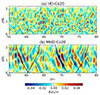 |
Fig. C.1. Torsional oscillation, i.e., temporal variation of the longitudinal (x) component of the mean flow δtUx(z, t) where the temporal average is subtracted, from (a) HD-Co20 and (b) MHD-Co20 cases. Black solid curves showcase paths of waves propagating upward and downward with the Alfvén velocity of the rms vertical field |
Taking a temporal derivative of Eq. (43), we have
![Mathematical equation: $$ \begin{aligned} \rho _{0} \frac{\partial ^{2} U_{x}}{\partial t^{2}} = -\frac{\partial }{\partial z} \left[ \frac{\partial }{\partial t} \left( \rho _0 \langle v^{\prime }_x v^{\prime }_z \rangle -\frac{ \langle B_{x}B_{z} \rangle }{4\pi } \right) \right]. \end{aligned} $$](/articles/aa/full_html/2025/11/aa56923-25/aa56923-25-eq259.gif) (C.1)
(C.1)
To estimate the temporal variation of the Reynolds and Maxwell stresses, we first consider the terms associated with the mean flow variation in Eqs. (2) and (3) to obtain
 (C.2)
(C.2)
 (C.3)
(C.3)
Taking a horizontal average of Eqs. (C.2 and C.3) and substituting them into Eq. (C.1), we have
![Mathematical equation: $$ \begin{aligned} \rho _0 \frac{\partial ^{2} U_{x}}{\partial t^{2}} \approx \frac{\partial }{\partial z} \left[\left( \rho _0 \langle v_z^2 \rangle + \frac{\langle B_{z}^{2} \rangle }{4\pi } \right) \frac{\partial U_{x}}{\partial z} \right]. \end{aligned} $$](/articles/aa/full_html/2025/11/aa56923-25/aa56923-25-eq262.gif) (C.4)
(C.4)
If we assume that ρ0⟨vz2⟩ and  vary more slowly in z than ∂Ux/∂z, the above equation can be reduced to a standard 1D wave equation
 (C.5)
(C.5)
where vA, z is the Alfvén velocity associated with the rms amplitude of the vertical magnetic field. If the MAC balance holds, the above equation (C.5) is reduced to the equation of torsional Alfvén waves whose propagation leads to a torsional oscillation restored by the Lorentz force of the fields perpendicular to the rotational axis (Braginskiy 1970).
Figure C.1 shows time-height plots of the torsional oscillation defined as
 (C.6)
(C.6)
for the cases HD-Co20 and MHD-Co20. Here, the temporal average is taken over a period T = 25 τ*. In the HD-Co20 case, the temporally fluctuating component of the mean flow is weak and the torsional oscillation patterns can hardly be identified with significant signal-to-noise ratio. In the MHD-Co20 case, on the other hand, we can unambiguously identify the torsional oscillation patterns in Fig. C.1b where the disturbances in the mean flow propagate vertically upward or downward with the Alfvén velocity vA, z. The typical amplitude of the torsional oscillation is δtUx/v* ≈ 0.05, which is approximately a few percent of the rms velocity fluctuation. It remains to be investigated how important these torsional oscillations are to the flow dynamics (e.g., Hori et al. 2023).
Appendix D: Physical origin of the Reynolds stress 
 |
Fig. D.1. Schematic illustration of the generation mechanisms of the Reynolds stress |


In this Appendix, we provide a physical explanation of the generation mechanism of the Reynolds stress  in slowly and rapidly rotating regimes.
We first consider a weak rotation regime (low-Co* regime). The Coriolis term in the equation of motion can be expressed as
![Mathematical equation: $$ \begin{aligned} \frac{\partial v_{x}^{\prime }}{\partial t}&= [...] -2\Omega _{0} v_{z}^{\prime }, \end{aligned} $$](/articles/aa/full_html/2025/11/aa56923-25/aa56923-25-eq271.gif) (D.1)
(D.1)
![Mathematical equation: $$ \begin{aligned} \frac{\partial v_{z}^{\prime }}{\partial t}&= [...]+2\Omega _{0} v_{x}^{\prime }. \end{aligned} $$](/articles/aa/full_html/2025/11/aa56923-25/aa56923-25-eq272.gif) (D.2)
(D.2)
Therefore, the sign of the Reynolds stress depends on whether the Coriolis force acts on vertical velocity  or on longitudinal velocity
  . Since vertical convective motions dominate over horizontal motions at low-Co* regime, negative Reynolds stress
  is selectively generated by Coriolis force acting on
  . This is schematically illustrated in Fig. D.1a.
Under a strong rotational influence (high-Co* regime), on the other hand, the above explanation cannot be applied because the geostrophic balance between the Coriolis force and the pressure gradient force is established. Since such a flow becomes invariant along the rotational (y) axis, it is convenient to consider the y-component of the vorticity  . Taking a curl of Eqs. (D.1 and D.2), we have
![Mathematical equation: $$ \begin{aligned} \frac{\partial \zeta _{y}^{\prime }}{\partial t} = [...]-\frac{2\Omega _{0}}{H_{\rho }} v_{z}^{\prime }. \end{aligned} $$](/articles/aa/full_html/2025/11/aa56923-25/aa56923-25-eq278.gif) (D.3)
(D.3)
This tells us that, due to the background density stratification, vertical motions cause an expansion or contraction of y vortices. The generation of positive (negative) y vorticity  in downflow (upflow) regions results in prograde propagation of the overall y-vortex columns, i.e., thermal Rossby waves. Now, a key to understanding the origin of the Reynolds stress is that the generation rate of this y-vorticity perturbation is stronger near the surface (where the density scale height Hρ is smaller) as expressed in Eq. (D.3). This causes vertically upward (downward) pressure gradient forces in downflow (upflow) regions because, in a geostrophic fluid, positive (negative) vortices
  are accompanied by negative (positive) pressure anomalies p′< 0 (> 0). In order to balance these additional vertical pressure gradient forces by the Coriolis force, retrograde (prograde) velocity perturbations
  are required in downflow (upflow) regions. Therefore, upflows and downflows are deflected to prograde and retrograde directions, respectively, leading to a net positive Reynolds stress
  . This positive Reynolds stress can be seen as a tilted pattern of the vortex columns, as illustrated in Fig. D.1b.
We note that the above explanation is similar to but different from the conventional explanation that the vortex columns are tilted in a prograde direction because the prograde phase speed of the thermal Rossby waves is faster near the surface than near the base (e.g., Busse 2002). Although this explanation is widely used within the community (e.g., Vasavada & Showman 2005; Glatzmaier et al. 2009), it has sometimes been criticized as unsatisfactory because the tilted pattern can be obtained as a linear eigenfunction of a global (normal) mode which propagates at a fixed phase speed everywhere (Takehiro 2008). Here, we provide an updated explanation for the origin of the Reynolds stress which does not rely on any nonlinear processes and thus is more satisfactory. Finally, it should be noted that our explanation can also be applied to incompressible thermal Rossby waves caused by the spherical curvature effect (e.g., Busse 2002) by simply replacing the compressional β effect, −2Ω0/Hρ, by the topographic β effect, 2Ω0(dlnh/dz), where h is the height of convective columns.
Appendix E: Origin of the spatial asymmetry in the y-vorticity pattern
A linear theory predicts that thermal Rossby modes at a fixed longitudinal wavenumber consist of positive and negative y-vorticity columns organized in an alternating pattern in longitude. However, our simulations show significant asymmetry between the columns with ζ′y > 0 and ζ′y < 0: That is, the columns with ζ′y > 0 are stronger and more spatially localized in longitude compared to those with ζ′y < 0 (see Figs. 18a and b). In this Appendix, we provide a physical explanation for the origin of this asymmetry based on a nonlinear effect.
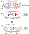 |
Fig. E.1. Schematic illustration explaining the origin of the asymmetry between counterclockwise and clockwise y vortices. (a) Vorticity generation rates in upflow and downflow regions. Red and blue dashed circles with arrows indicate the generations of negative and positive y vortices (corresponding to higher and lower pressure perturbations). The vorticity generation is stronger (represented by larger circle size) inside the low-pressure column with ζy′> 0 due to the nonlinear effect. (b) Directions of the pressure gradient forces (red arrows) and the flows required to balance these pressure gradient forces by their Coriolis forces (black arrows). (c) Spatial pattern of the y vortices modified by the nonlinear effect. In all panels, the rotational axis points toward us. |
We begin by examining the y-component of the vorticity equation
![Mathematical equation: $$ \begin{aligned} \frac{\partial \zeta ^{\prime }_y}{\partial t} = [...] + \beta _{\rm nonlin} v^{\prime }_z, \end{aligned} $$](/articles/aa/full_html/2025/11/aa56923-25/aa56923-25-eq283.gif) (E.1)
(E.1)
where the definition of the compressional β effect is slightly modified to include the nonlinear advective term as
 (E.2)
(E.2)
This means that the compressional β effect is effectively enhanced in regions with ζ′y > 0 and is suppressed where ζ′y < 0. Now, let us consider upflow and downflow regions located between positive and negative y-vorticity columns. As already explained in Appendix D, positive (negative) y-vorticity perturbations are generated in downflow (upflow) regions. What is crucial here is that this vorticity generation becomes stronger (weaker) inside the positive (negative) y-vorticity columns, as schematically illustrated in Fig. E.1a. Since positive (negative) pressure anomalies are involved with negative (positive) y vortices in a geostrophic fluid, additional pressure gradient forces are induced in a longitudinal direction. As shown in Fig. E.1b, these additional pressure gradient forces are directing retrograde in upflow/downflow regions and prograde inside the positive y-vorticity columns. In order to balance these additional pressure gradient forces by the Coriolis force, vertical velocity perturbations are required. Consequently, downflows (upflows) are enhanced (weakened) and upflow regions are shifted toward the prograde direction by this nonlinear effect. As is depicted in Fig. E.1c, these modifications lead to a more spatially localized structure for columns with ζ′y > 0, while columns with ζ′y < 0 become more spatially extended.
All Tables
All Figures
|
Fig. 1. Sketch of the local Cartesian model of the stellar convection zone. The local f-plane box is located at the equator, where the x, y, and z axes point to the longitudinal, latitudinal, and radial directions, respectively. |
| In the text | |
|
Fig. 4. Same as Fig. 3 but from the simulation cases HD-Co2 and MHD-Co2. An animation of this figure is available online. |
| In the text | |
|
Fig. 2. Temporal evolution of the volume-integrated kinetic and magnetic energies, Ekin (dashed curves) and Emag (solid curves), from the MHD runs. Different colors represent the results with different Co*. |
| In the text | |
|
Fig. 3. Temporal snapshots of (a) the vertical velocity, vz, from case HD-Co1, (b) vz from case MHD-Co1, and (c) the vertical magnetic field, Bz, from MHD-Co1 in the statistically stationary states at t ≈ 80 τ*. The top and middle panels show the horizontal cuts near the top surface, z = 2.2 Hr, and in the middle convection zone, z = 1.2 Hr. The bottom panels show the vertical cuts at y = 0. An animation of this figure is available online. |
| In the text | |
|
Fig. 5. Same as Fig. 3 but from the simulation cases HD-Co5 and MHD-Co5. An animation of this figure is available online. |
| In the text | |
|
Fig. 6. Same as Fig. 3 but from the simulation cases HD-Co10 and MHD-Co10. An animation of this figure is available online. |
| In the text | |
|
Fig. 7. Same as Fig. 3 but from the simulation cases HD-Co20 and MHD-Co20. An animation of this figure is available online. |
| In the text | |
|
Fig. 8. Two-dimensional kinetic energy spectra shown in a horizontal wavenumber space (kx, ky) in the middle convection zone (z = 1.1 Hr) for (a) weakly rotating and (b) rapidly rotating cases. The top and bottom rows show the results of HD and MHD simulations, respectively. The insets show cuts of the same spectra at fixed ky, where the red, blue, green, and gray curves correspond to cuts through kyLy/2π = 0, 1, 2, and 3. |
| In the text | |
|
Fig. 9. (a) Kinetic energy spectra, |
| In the text | |
|
Fig. 10. Profiles of the rms convective velocity, vrms, and the Alfvén velocity of the rms magnetic field, |
| In the text | |
|
Fig. 11. Entropy perturbations, s′1, in our simulations. (a,b) Temporal snapshots of s′1 weighted by the background density, ρ0, at fixed height (z = 1.2 Hr) and latitude (y = 0) from weakly rotating simulations HD-Co2 and MHD-Co2. (c,d) Same as panels a and b but from rapidly rotating cases HD-Co20 and MHD-Co20. (e) Volume-averaged rms entropy perturbation, |
| In the text | |
|
Fig. 12. Profiles of the superadiabaticity, δ. (a–d) Vertical profiles of δ for different Co*. Blue and red curves represent the results from HD and MHD simulations. (e) Volume-averaged values of superadiabaticity, |
| In the text | |
|
Fig. 13. Force balances in our simulations. (a) RMS amplitudes of the forces, Frms. Here, Frms is calculated such that Frms2 = V−1∫V(Fx′2 + Fy′2 + Fz′2)dV. Yellow, red, green, blue, and purple colors represent the nonlinear advection, pressure gradient, buoyancy, Coriolis, and Lorentz forces. The top and bottom panels show the HD and MHD simulations, respectively. (b) RMS amplitudes of the y-averaged forces, |
| In the text | |
|
Fig. 14. (a) Normalized kinetic energy spectra, |
| In the text | |
|
Fig. 15. Profiles of the mean flows, Ux(z). (a–d) Vertical profiles of Ux(z) for different Co*. Blue and red colors represent the results from the HD and MHD simulations. (e) Vertical shear amplitudes of the mean flow, ΔUx = Ux(zmax)−Ux(zmin), as a function of Co*. |
| In the text | |
|
Fig. 16. Profiles of the Reynolds and Maxwell stresses, defined by Eq. (44). Positive and negative values correspond to the upward and downward AMT. (a–d) Vertical profiles of the Reynolds stress, ℛxz, for different values of Co*. Blue and red colors represent the results from the HD and MHD cases. Green curves show the vertical profiles of the Maxwell stress, ℳxz, and the dashed black curves indicate the sum ℛxz + ℳxz in the MHD simulations. (e) Volume-averaged Reynolds and Maxwell stresses, |
| In the text | |
|
Fig. 17. Breakdown of the contributions from the ky = 0 and ky ≠ 0 components to the Reynolds and Maxwell stresses. (a,b) Volume-averaged Reynolds stress, |
| In the text | |
|
Fig. 18. Snapshots of the y-averaged quantities from MHD simulations with Co* = 2, 5, 10, and 20. Each panel, from top to bottom, displays the y-averaged profiles of the x velocity, |
| In the text | |
|
Fig. 19. (Top) Correlations between the Maxwell stress, |
| In the text | |
|
Fig. 20. Volume-integrated (a) kinetic energy, |
| In the text | |
|
Fig. C.1. Torsional oscillation, i.e., temporal variation of the longitudinal (x) component of the mean flow δtUx(z, t) where the temporal average is subtracted, from (a) HD-Co20 and (b) MHD-Co20 cases. Black solid curves showcase paths of waves propagating upward and downward with the Alfvén velocity of the rms vertical field |
| In the text | |
|
Fig. D.1. Schematic illustration of the generation mechanisms of the Reynolds stress |
| In the text | |
|
Fig. E.1. Schematic illustration explaining the origin of the asymmetry between counterclockwise and clockwise y vortices. (a) Vorticity generation rates in upflow and downflow regions. Red and blue dashed circles with arrows indicate the generations of negative and positive y vortices (corresponding to higher and lower pressure perturbations). The vorticity generation is stronger (represented by larger circle size) inside the low-pressure column with ζy′> 0 due to the nonlinear effect. (b) Directions of the pressure gradient forces (red arrows) and the flows required to balance these pressure gradient forces by their Coriolis forces (black arrows). (c) Spatial pattern of the y vortices modified by the nonlinear effect. In all panels, the rotational axis points toward us. |
| In the text | |
Current usage metrics show cumulative count of Article Views (full-text article views including HTML views, PDF and ePub downloads, according to the available data) and Abstracts Views on Vision4Press platform.
Data correspond to usage on the plateform after 2015. The current usage metrics is available 48-96 hours after online publication and is updated daily on week days.
Initial download of the metrics may take a while.