| Issue |
A&A
Volume 704, December 2025
|
|
|---|---|---|
| Article Number | A53 | |
| Number of page(s) | 17 | |
| Section | Numerical methods and codes | |
| DOI | https://doi.org/10.1051/0004-6361/202554688 | |
| Published online | 03 December 2025 | |
Stream automatic detection with convolutional neural networks
1
Departamento de Astronomía, Universidad de La Serena,
Raúl Bitrán N° 1305,
La Serena,
Chile
2
Departamento de Física, Universidad Técnica Federico Santa María,
Avenida España 1600,
2390123
Valparaíso,
Chile
3
Max-Planck-Institut für Astrophysik,
Karl-Schwarzschild-Str. 1,
85748,
Garching,
Germany
4
Cardiff Hub for Astrophysics Research and Technology, School of Physics and Astronomy, Cardiff University,
Queen’s Buildings,
Cardiff
CF24 3AA,
UK
5
Center for Theoretical Astrophysics and Cosmology, Department of Astrophysics, University of Zurich,
Switzerland
6
Astrophysics Research Institute, Liverpool John Moores University,
146 Brownlow Hill,
Liverpool
L3 5RF,
UK
7
Department of Physics and Astronomy “Augusto Righi,” University of Bologna,
via Gobetti 93/2,
40129
Bologna,
Italy
8
INAF, Astrophysics and Space Science Observatory Bologna,
Via P. Gobetti 93/3,
40129
Bologna,
Italy
★ Corresponding author: This email address is being protected from spambots. You need JavaScript enabled to view it.
Received:
21
March
2025
Accepted:
15
September
2025
Abstract
Context. Galactic halos host faint substructures such as stellar streams and shells, which provide insights into the hierarchical assembly history of galaxies. To date, such features have been identified in external galaxies by visual inspection. However, with the advent of larger and deeper surveys and the associated increase in data volume, this methodology is becoming impractical.
Aims. Here we aim to develop an automated method to detect low surface brightness features in galactic stellar halos. Moreover, we seek to quantify the performance of this method when considering progressively more complex datasets, including different stellar disc orientations and redshifts.
Methods. We have developed the stream automatic detection with convolutional neural networks (SAD-CNNs) models. This tool was trained on mock surface brightness maps obtained from simulations of the Auriga Project. The model incorporates transfer learning, data augmentation, and balanced datasets to optimise its detection capabilities at surface brightness limiting magnitudes ranging from 27 to 31 mag arcsec−2.
Results. The iterative training approach, coupled with transfer learning, allowed the model to adapt to increasingly challenging datasets, achieving precision and recall metrics above 80% in all considered scenarios. The use of a well-balanced training dataset is critical for mitigating biases and ensuring that the CNN accurately distinguishes between galaxies with and without streams.
Conclusions. SAD-CNN is a reliable and scalable tool for automating the detection of faint substructures in galactic halos. Its adaptability makes it well suited to future applications that would include the analysis of data from upcoming large astronomical surveys such as LSST and JWT.
Key words: methods: numerical / Galaxy: halo / galaxies: dwarf / galaxies: structure
© The Authors 2025
 Open Access article, published by EDP Sciences, under the terms of the Creative Commons Attribution License (https://creativecommons.org/licenses/by/4.0), which permits unrestricted use, distribution, and reproduction in any medium, provided the original work is properly cited.
This article is published in open access under the Subscribe to Open model. This email address is being protected from spambots. You need JavaScript enabled to view it. to support open access publication.
1 Introduction
The current paradigm of galaxy formation postulates that the accretion of material from the surrounding environment drives the mass growth of galaxies (Searle & Zinn 1978; White & Rees 1978; White & Frenk 1991; Johnston et al. 1996, 2008; Li & Helmi 2008). Galaxies are not singular bodies, they are surrounded by vast halos that are home to a variety of faint features indicative of their intricate assembly history (Helmi et al. 1999; Helmi 2008; Cooper et al. 2010; Pillepich et al. 2015). These low surface brightness features (LSBFs), which often manifest as stellar streams, shells, and plumes, are either the direct or indirect results of previous interactions. Thus, LSBFs provide crucial information about the accretion history of a galaxy. In particular, streams and shells are the remnants of past accretion processes that feed the hierarchical growth of galaxies (Ibata et al. 1994; Hibbard & Mihos 1995; Johnston et al. 1996; Majewski et al. 1999; Helmi et al. 2003a; McConnachie et al. 2009; Martínez-Delgado et al. 2010).
Stellar streams are long, narrow coherent structures composed of stars orbiting galaxies and are typically stretched along the orbital path of a progenitor satellite that is gradually disrupted by the gravitational forces of its host galaxy (Johnston et al. 2008). These streams are the result of interactions between galaxies and ongoing accretion processes. Several studies have attempted to characterise the accretion history the Milky Way by analysing substructures in the six-dimensional phase space distribution of local volumes, which allows not only for the detection of phase-mixed stellar streams but also the placement of constraints on the structure, size, and orbital histories of the progenitors (Helmi & White 1999; Helmi et al. 2003b; Meza et al. 2005; Gómez & Helmi 2010; Belokurov et al. 2018; Malhan et al. 2018; Helmi 2020; Li et al. 2021). The discovery and characterisation of these faint substructures in the Milky Way have been greatly advanced thanks to surveys such as Gaia (Gaia Collaboration 2018; Ibata et al. 2021). The information provided by surveys combined with the mapping of the outer halo with photometric and spectroscopic surveys (Bonaca & Price-Whelan 2025) has enabled a comprehensive view of the merging history of our Galaxy for the first time.
Regarding the other two highlighted LSBFs, shells are sharp, arc-like stellar features that are typically generated during eccentric mergers, where a satellite galaxy plunges nearly radially into the host, producing interleaved shells of debris at successive apocentres (Quinn 1984; Lotz et al. 2008; Villalobos & Helmi 2008). In contrast, plumes are more diffuse, irregular structures that often result from minor mergers or tidal interactions, and they may lack the coherent morphology of streams or shells (Janowiecki et al. 2010; Martínez-Delgado et al. 2010).
The study of these faint substructures in external galaxies presents important challenges mainly concerned with their detectability (Belokurov et al. 2006; Martínez-Delgado et al. 2010; Atkinson et al. 2013; Morales et al. 2018; Shipp et al. 2018; Gordon et al. 2024). The detection and characterisation of an LSBF is a highly complex task due to their extremely faint brightness. Indeed, deep observations with a surface brightness limit deeper than 29 mag arcsec−2 in the r-band are required (Bullock & Johnston 2005; Cooper et al. 2013; Conselice et al. 2000; Ji et al. 2014; Fliri & Trujillo 2016; Morales et al. 2018; Hood et al. 2018; Mancillas et al. 2019; Gordon et al. 2024). Previous studies have started to provide different censuses about tidal streams and faint stellar substructures in external galaxies, which are crucial for understanding their prevalence. Atkinson et al. (2013), using a sample of 1781 galaxies, reported that approximately 26% of galaxies with stellar masses exceeding 1010.5 M⊙ exhibited detectable tidal features with a μlim ≈ 27.7 mag arcsec−2. Expanding on these findings, Duc (2017) explored a broader census through the MATLAS survey in a sample of 360 massive nearby galaxies and revealed a higher fraction of galaxies, reaching 40%, with observed faint substructures. A more recent study based on the RESOLVE survey (Hood et al. 2018), which reaches an r-band depth of ∼27.9 mag arcsec−2 for a sample of 1048 galaxies, identified faint features in ∼17% of their galaxies. Morales et al. (2018) reported a limiting surface brightness of  for their sample of 232 images. In particular Walmsley et al. (2019) detected tidal features in a dataset covering approximately 170 deg2 with a limiting surface brightness of
  . Notably, Bílek et al. (2020) found that the presence of these faint features correlates with the mass of the host galaxy and is influenced by environmental factors. These detection rates highlight the difficulties in establishing a comprehensive census of faint features, which may be affected by factors such as the depth of the survey, the quality of the data, and the specific techniques used for identification. Moreover, the nature of these structures, which can be distorted or disrupted by various factors, further complicates their study. Thus, advanced techniques, such as stacking of multiple images, pixel-level analysis, and multi-gauss expansion (MGE) model are used for the detection and characterisation of tidal streams (Kado-Fong et al. 2018; Sola et al. 2022; Miró-Carretero et al. 2023; Rutherford et al. 2024).
State of the art cosmological simulations such as Auriga (Grand et al. 2017) and FIRE (Hopkins et al. 2018) have significantly advanced our understanding of the hierarchical growth of galaxies and the formation of their stellar halos. These simulations track the accretion histories of galaxies, allowing researchers to study the origins and properties of stellar streams in a cosmological context. Several works have utilised cosmological simulations to explore stellar halos and their properties, which have provided valuable insights into these complex structures (Johnston et al. 2008; Cooper et al. 2010; Tumlinson 2010; Helmi et al. 2011; Tissera et al. 2013, 2014; Erkal & Belokurov 2015; Amorisco 2017; Monachesi et al. 2019; Vera-Casanova et al. 2022; Martin et al. 2022; Valenzuela & Remus 2024; Kado-Fong et al. 2022; Shipp et al. 2023; Gonzalez-Jara et al. 2025; Tau et al. 2025; Riley et al. 2025; Shipp et al. 2025). These theoretical approaches offer diverse insights into the formation and evolution of faint features, providing a basis for understanding the processes that drive the assembly history of galaxies. Recent work has focused on specific aspects of stellar halo formation. For example, Erkal & Belokurov (2015); Walder et al. (2025) investigated how properties of stellar tidal streams can provide properties of the dark halo, while Amorisco (2017) explored the connection between a merger history and the properties of the accreted stellar halo. Vera-Casanova et al. (2022) used the Auriga simulations to study stellar halos in Milky Way-mass galaxies, predicting the fraction of stellar streams detectable at different surface brightness limits. Martin et al. (2022) emphasised the importance of including realistic observational conditions in simulations, showing how such factors can significantly impact the detectability of faint features. Similarly, Kado-Fong et al. (2022) have demonstrated how stream morphology and spatial distribution can constrain the assembly history of halos in cosmological simulations.
The next generation of surveys such as LSST and EUCLID (Ivezic et al. 2019; Euclid Collaboration: Aussel et al. 2025) are about to dramatically increase the volume of data available to researchers. While in the past, it was possible to visually inspect images to identify and classify different features of interest, this methodology is progressively becoming infeasible. As a result, the upcoming burst of data motivates the development of automated tools, particularly those employing machine learning techniques, to extract and efficiently analyse information from these large datasets. Such tools applied to the forthcoming surveys could allow for the detection and characterisation of a large number of stellar streams and enable a statistical study based on the properties and prominence of these substructures. Accurately quantifying the fraction of galaxies that present an LSBF as a function of limiting surface brightness magnitude would not only allow individual galaxy merger histories to be constrained but could also provide important constraints on the galaxy merger rate as a function of time (Vera-Casanova et al. 2022; Martin et al. 2022; Miro-Carretero et al. 2025).
Convolutional neural networks (CNNs) belong to a class of neural networks commonly used for processing array representations, such as 1D sequences, 2D images, or 3D videos (LeCun et al. 2015). In the context of images, they have been widely applied to tasks such as recognition (Bickley et al. 2021), segmentation (Farias et al. 2020), and style transfer (Gatys et al. 2016). The main idea behind CNNs is automatically extracting relevant features from images and condensing this information into a feature map. The model then learns the non-linear combinations of these features through a training process, enabling predictions for new input data. In recent years, CNNs have become powerful tools for automated feature extraction and pattern recognition in astronomy. They are applied to tasks such as galaxy morphology classification (Walmsley et al. 2019; Farias et al. 2020; Sánchez-Sáez et al. 2021; Bickley et al. 2021) and the identification of faint features (Baxter et al. 2021; Gordon et al. 2024; Fontirroig et al. 2025). By exploiting the enormous amount of data produced by modern astronomical surveys, CNNs provide an efficient and powerful approach to analysing and interpreting astronomical datasets. Recently, Gordon et al. (2024) advanced this field by employing CNNs to classify tidal features into distinct categories, highlighting the potential of automated methods for analysing faint substructures.
In this study, we use the capabilities of CNNs to automate the detection of faint substructures, specifically stellar streams, in galactic halos. By training a CNN on simulated surface brightness maps generated from the Auriga Project simulation dataset, we aim to develop a robust and efficient methodology to identify and characterise stellar streams. Our approach accelerates the process of analysing complex astronomical datasets and allows for the exploration of intricate structures within galactic halos.
This paper is organised as follows. In Section 2, we introduce the simulation and the method employed to make the training samples. Additionally, we describe the CNN utilised in this process. In Section 3, we explain the methodology for training step by step. In Section 4 we discuss the training process, while in Section 5 we present the results obtained from random samples of images. Finally, in Section 6, we summarise the main results obtained in this work.
2 The Auriga simulations
The Auriga project is a suite of cosmological zoom-in simulations designed to produce reasonably isolated galaxies in the mass range of the Milky Way (Grand et al. 2017, 2024). These simulations consist of thirty (30) zoom halo simulations from the EAGLE project (Schaye et al. 2015). The halos were selected at z = 0 to be Milky Way-mass systems (1 < M200/1012M⊙ < 2) and to satisfy an isolation criterion based on the tidal isolation parameter τiso. This ensures that the main halo is not a substructure of a more massive system and does not reside in a dense cluster environment, while remaining sufficiently isolated from any neighbouring halo more massive than 3% of its mass within nine virial radii (See Eq. (1) in Grand et al. 2017). Performed in the framework of ΛCDM cosmology with parameters Ωm = 0.307, Ωb = 0.048, ΩΛ = 0.693, and Hubble constant H0 = 100 h km s−1 Mpc−1, h = 0.6777 (Planck Collaboration XVI 2014).
The simulations have a resolution of baryonic mass particles of ∼5 × 10⁴ M⊙ and resolution for dark matter particles ∼4 × 10⁵ M⊙, with a comoving softening length of 369 pc at z = 1, after which the softening is kept constant in physical units. These correspond to ‘level 4’ of Auriga Project. These simulations were run using the AREPO code on a periodic cube with a side length of 100 cMpc (Springel 2010; Pakmor et al. 2016). arepo solves the magnetohydrodynamical equations and integrates models of galaxy formation (Vogelsberger et al. 2013; Grand et al. 2017), incorporating sub-grid models for baryonic processes such as star formation (Springel & Hernquist 2003).
The Auriga model assigns a single stellar population to each stellar particle. This assignment occurs every time there is a star formation episode, ensuring that each stellar particle is associated with a specific stellar population. The properties of these stellar populations account for mass loss and chemical enrichment from Type Ia supernovae and asymptotic giant branch stars, along with their respective ages and masses. These populations are characterised by their mass, age, mass-loss history, and chemical abundance patterns. The interstellar medium is modelled using the subgrid multiphase approach introduced by Springel & Hernquist (2003). It describes the dense and cold gas of the interstellar medium with an effective equation of state that originates from the balance of gas cooling and heating by supernova feedback. The photometric bands U, B, V, g, r, i, z, and K from Bruzual & Charlot (2003) are calculated for each stellar particle, without accounting for dust extinction.
The Auriga simulations are an excellent laboratory for studying the properties of stellar halos due to their high resolution (Grand et al. 2017; Monachesi et al. 2016, 2019; Fattahi et al. 2020; Pu et al. 2025). In particular, Monachesi et al. (2019) presented a detailed comparison between simulated halos and those observed in the nearby Universe with the HST telescope within the Galaxy Halos, Outer discs, Substructure, Thick discs, and Star clusters (GHOSTS) project, showing that the parameters that characterise the Auriga stellar haloes, as well as their scatter, are generally in good agreement with the observed properties of nearby stellar haloes. Simpson et al. (2018), showed that the luminosity function of satellites at redshift zero closely matches the observed luminosity function of both the Milky Way and Andromeda (M31). This agreement holds for satellites with stellar masses above 106 M⊙, which aligns with the resolution used in these studies. Vera-Casanova et al. (2022) showed that approximately 87% of the simulated halos exhibit stellar streams at redshift z = 0, across a wide range of surface brightness limits. However, these streams do not necessarily originate from the most massive accretion events, as even satellites disrupted several gigayears ago can leave detectable tidal features that persist until the present time. Riley et al. (2025) and Shipp et al. (2025) further explored the disruption of satellite galaxies around the Auriga haloes. They found that the distribution of streams in pericentre-apocentre space overlaps significantly with the Milky Way intact satellite population. However their results suggest that either cosmological simulations, such as Auriga, are disrupting satellites far too readily, or that the Milky Way’s satellites are more disrupted than current imaging surveys have revealed.
Summarising, in this work we generate simulated surface brightness maps using a sample of 30 Milky Way-like halos from the Auriga suite. These are fully self-consistent cosmological magnetohydrodynamical simulations run within a Λ-CDM cosmology. The galaxies are characterised by stellar masses of 2-10 × 1010 M⊙ and disc-dominated morphologies, with a baryonic mass resolution of the ≈ 5 × 10⁴ M⊙. All halos were chosen to be reasonably isolated at redshift z = 0.
3 Methodology
We used the Auriga simulations to generate surface brightness maps of late-type galaxies at different redshifts, inclinations, and surface brightness limits. These images were used to train a CNN to rapidly and efficiently identify LSBFs. Our training is done in stages, increasing the complexity behind the detectability of these features at every step. As a result, we seek to understand the main limitations behind this type of approach. Our training sets consist of ∼10000 different images with different projections and rotations of galaxies. In this sample, we indicated the presence or absence of a stellar stream by visual inspection of the images (see Sect. 3.1).
3.1 Surface brightness maps
Each stellar particle in the Auriga simulation represents a different stellar population, with a given mass, age, and metallicity. As discussed in Sect. 2, each particle has determined its luminosity in the U, V, B, K, g, r, i, and z bands, calculated based on its mass, age, and metallicity. These luminosities are derived following the methodology described in Bruzual & Charlot (2003). To mitigate the effects of dust extinction, and to have a better tracer of the underlying mass distribution, previous observational works (e.g. Atkinson et al. 2013; Morales et al. 2018; Martin et al. 2022; Miró-Carretero et al. 2023; Martínez-Delgado et al. 2023; Smercina et al. 2023), have focused their analysis on surface brightness (SB) maps obtained in the photometric r-band. Auriga does not include a self-consistent dust model, meaning that these luminosities are computed without the direct effects of dust attenuation. Thus, for the CNN training, we employed SB Maps derived from the luminosity distribution of each simulated galaxy in this band. We considered all stellar particles located within a radial distance of 150 kpc from the galactic centre. In this work, the galactic centre is defined following Vera-Casanova et al. (2022), where it is determined by identifying the particle most bound to the system.
Building on the detection rates reported in Vera-Casanova et al. (2022) and Miro-Carretero et al. (2025), we note that LSBF become increasingly prominent for surface brightness limits ≥27 (mag arcsec−2). Based on this, to simulate different observational depths, we apply surface brightness limits (μlim) by setting all pixel values fainter than the chosen limit to zero (i.e. masking them). Specifically, we define μlim as the surface brightness value in mag arcsec−2 corresponding to the minimum detectable pixel value in the map. We apply limits ranging from 27 to 33 mag arcsec−2, in steps of one magnitude, where features fainter than the μlim depth are undetectable.
To assure uniformity and comparability between the generated SB maps, we performed a normalisation process before using them to train the CNN. Each map was converted into a FITS image format and then normalised by its maximum pixel luminosity value, resulting in pixel values ranging from zero to one. The normalisation procedure effectively standardises the intensity distribution across all maps, independent of the specific limiting magnitude. This strategy allows us to mitigate biases due to differences in magnitudes in the analysed SB maps and ensures that the CNN learns to discern faint substructures rather than being influenced by the typical low SB values associated with these substructures. In addition, all images were generated considering 300×300 pixels size. This corresponds to a physical resolution of 1 kpc per pixel. This standardised resolution facilitates consistency in feature recognition and analysis across the entire dataset. We note that, when mocking observations from different instruments, the spatial resolution and associated observational errors may affect the detectability of some of the faintest features that exist (Miro-Carretero et al. 2025). This, nevertheless, does not affect the results of our training process.
The generated SB maps were utilised to identify LSBFs in each galaxy. This was done by visual inspection of each image, following the procedure described in Vera-Casanova et al. (2022). Specifically, images without any discernible features were assigned a value of zero, while images exhibiting faint structures were assigned a value of one. During this procedure we decided to not classify low SB satellites that still gravitationally bound as faint features. For this procedure, we made individual selections between co-authors, followed by multiple iterations and discussions over the selection. This collaborative process eventually culminated in a shared visual inspection.
3.2 Deep learning
A CNN employs a convolutional operator to process images by applying a discrete linear transformation over the input data matrix. In this case, the input data consists of images representing SB maps of our simulated galaxies. CNNs are typically composed of four fundamental components: convolutional layers, regularisation layers, clustering layers, and fully connected layers. These layers work together to extract meaningful features from the input data, and the final layer uses these features to generate predictions. Regularisation layers, such as the exclusion layer, are used to improve network generalisation and mitigate overfitting by randomly excluding neurons during training.
Through a training process, the network learns to capture nonlinear combinations of features, allowing accurate predictions to be made on new input data. As previously stated, the CNN applies a discrete linear transformation over the input image and provides weights for every discrete position of the corresponding matrix. During this process it applies multiple combinations of different kernels to capture different features and patterns in the input images, helping the classification process (see Dumoulin & Visin 2016). The input data for the convolutional layers consist of a three-dimensional matrix, two spatial dimensions, and a third dimension with intensity values. This last dimension is usually called the dimension channel, which has information on quantities such as colours or brightness intensities.
We utilised the Xception (Chollet 2016) CNN architecture to identify low SB features on mock galaxy images. The Xcep-tion model uses depthwise separable convolution, also called ‘separable convolution’, a technique that factorises standard convolutions into two separate operations: a depthwise convolution, which applies spatial filtering independently to each input channel, followed by a pointwise convolution, which combines information across channels. This approach reduces computational cost while maintaining high classification performance. This approach is also computationally efficient and helps reduce the number of parameters in the network. The design choice allows Xception to optimise model size, computational complexity, and performance. In this work, we used a sigmoid function output to deliver one value per class for each of the examples. The output layer scales the network output between 0 and 1. This allowed us to interpret the results as the probability that a given image contains a feature learned during the training process. (For a more detailed explanation, see Chollet 2016.)
3.3 Training method and metrics
The training process consists of a minimisation problem to fit the data. As previously discussed, during this process different kernels, and their associated weights, are considered to find the optimal configuration that best summarises and classifies the images. A common approach is to initialise the weights with random values and then, through a trial and error process, optimise these weights to recognise the images. To conduct the trial and error process, we need to divide the data into three independent sets: Training set, Validation set, and Test set. We allocated 80%, 10%, and 10% of the total sample of images to each set, respectively. The training set is used directly to adjust the network’s weights, improving classification through an iterative process. The validation set was used during training to indirectly evaluate the performance of the model and adjust the parameters as needed, while the test set, composed of previously unseen images, is reserved for the final evaluation of the accuracy of the model.
To guarantee the robustness of our model, we balanced the training set so that it contains an equal number of images with and without LSBF at each surface brightness limit. This procedure is essential to prevent biases in the training process and to ensure that the model learns to accurately distinguish between the two classes under varying conditions. To achieve this, we applied a data augmentation process, which consists of simple geometric transformations, including rotations and reflections of the images themselves. It is important to emphasise that these transformations are purely two-dimensional operations applied to the mock images and do not correspond to a physical re-orientation of the simulated galaxies. Although repeated augmentation may introduce redundancy, the whole number of augmented samples in our training set is still less than twice the original size dataset. This level is generally considered moderate and not excessive in image classification tasks (Perez & Wang 2017). In this way, we increased the diversity of the training data, which helped the model to better generalise the unseen data. Figure 1 shows an example of this procedure. Importantly, the mock images selected to perform the data augmentation process are randomly selected. This approach helps mitigate the natural bias introduced by galaxies observed at deeper SB limits, ensuring a more accurate evaluation of the ability of the model to detect LSBF in different scenarios.
The model classifies an image as containing an LSBF if the predicted probability exceeds a threshold of 0.5; otherwise, it is classified as not containing such features. To assess the classification performance, we defined four possible outcomes based on visual classification:
True positives (TP): The network correctly identifies the presence of an LSBF.
False positives (FP): The network incorrectly classifies an image as containing an LSBF when it does not.
True negatives (TN): The network correctly identifies the absence of an LSBF.
False negatives (FN): The network fails to detect an LSBF that is actually present.
The results of the trained network are evaluated using various performance metrics, which are quantitative measures used to assess performance on specific tasks. They are also used by the model to help guide the iterative process of improving model design and performance. Common metrics include accuracy, precision, recall, and the F1-score. Our primary metric for evaluation, namely accuracy, was calculated as
 (1)
(1)
Accuracy measures the percentage of instances correctly classified from the total dataset, and it is commonly used in classification tasks. Precision, defined as
 (2)
(2)
represents the ratio of true positive predictions to all positive predictions. Recall,
 (3)
(3)
measures the proportion of true positive predictions out of all actual positive instances in the dataset.
Finally, we also used the F1-score metric, which combines precision and recall into a single value:
 (4)
(4)
The F1-score provides a balanced assessment of the performance model, especially in situations where precision and recall need to be balanced. It is defined as the harmonic mean of precision and recall, ranging from 0 to 1, where 1 indicates perfect precision and recall, and 0 indicates that the model has completely failed to identify positive cases.
In this work, we apply a technique known as transfer learning (TL), which involves reusing knowledge learned from one dataset to improve performance on a related but different dataset. For instance, in the context of galaxy morphological classification, weights trained on astronomical images can serve as a starting point. Additionally, studies have demonstrated that TL can even be effective when using weights pre-trained on unrelated datasets (e.g. Iman et al. 2023). In our case, we initialise our model with weights pre-trained on the ImageNet dataset (Deng et al. 2009), which contains a broad range of labelled images across various categories. This approach allows the network to start with a general understanding of image features, improving the efficiency of training on our specific task. To train the network, we use the Adam optimiser (Kingma & Ba 2014) with a learning rate of 0.0001, running the model for up to 200 epochs. To prevent overfitting, we employ early stopping. This method monitors a selected metric (such as validation loss) and halts training if no improvement is observed within a specified number of epochs1 (Keras Team 2022). When incorporating new data into our analysis, such as images of galaxies with varying inclinations, we concatenate a random 20% of the previous training set with the next one and retain the pre-trained weights from the earlier training stages. This approach ensures that the model builds on previously learned features while adapting to the additional data. The resulting network combines the weights from previous training sessions with the new dataset, providing a robust model capable of generalising to more diverse conditions.
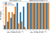 |
Fig. 1 Example of data augmentation applied to the test sample of images with and without stellar streams. The left panel shows the original test sample distribution at z = 0, where images are unevenly distributed across SB limits ( |

3.4 Training sets definition
A summary of our training procedure is presented in the scheme of Figure 2. Our training methodology follows a stepwise approach, where the model is first trained on a simpler dataset and then progressively exposed to more complex cases. At each training step, the effectiveness of the trained model was evaluated using a test set. As a first step, we trained the model only considering edge-on galaxies at z = 0. This is the simplest possible configuration as it avoids issues associated with the extended light distribution of the discs and their internal structure. Once tested, the CNN was further trained and tested using a large sample of edge-on galaxies obtained at different redshifts. We finally generated a sample of late-type galaxies with different inclinations. This allowed us to test the performance of our previously trained network on this more challenging configuration. Based on this evaluation, we refined the model by incorporating images of inclined galaxies into the training process, which allowed it to generalise better to different orientations. To carry out this iterative procedure, we generated different datasets. These sets are described below.
Group I comprises 210 images of our simulated galaxies in an edge-on projection, all at z = 0. We emphasise that from each Auriga model, several images are obtained by systematically varying the limiting SB magnitude. These images serve as the foundation for the initial training phase. We consider this to be the most simple case for the network, as we can observe the halo without having the disc covering a large area of the image. It also eliminates potential problems with disc features, such as spiral arms. This group encompassed variations of edge-on galaxies achieved through rotations about the symmetry axis of our disc galaxies. Specifically, rotations of 30°, 45°, 60°, and 90° were applied to the original 210 images, resulting in a total of 1050 distinct FITS images. Each rotation introduced unique configurations of the LSBF and satellites in the configuration space, as shown in Figure 3. In particular, some rotations, such as the 30° rotation depicted in the second column of the upper row, led to scenarios where the stellar streams are hard to disentangle from the stellar halo component. We randomly selected 10% of the total images (105) to form an independent test set. The remaining images were used for training, with additional data augmentation, increasing the final training set to 1764 images. This enriched dataset enables the CNN to learn a broader variety of geometric configurations while maintaining the physical consistency of each image.
In the subsequent learning phase, a new sample of images was introduced, Group II, comprising galaxies within the following redshifts: z = [0.024, 0.049, 0.074, 0.099, 0.126, 0.153, 0.180, 0.214, 0.244, 0.276]. This group consisted of 2100 images, representing galaxies at different stages of late evolution, influenced by their merger history. An example of such images is shown in Figure 3 using the same halo rotated previously. Ten percent of this sample was separated into a test set. After the separation, we augmented the data by applying rotations and random flips to the images, resulting in 3664 images.
Finally, the last learning phase introduced galaxies, with varying inclinations of the disc symmetry axis for the line of sight. This group, Group III, incorporated inclinations of 15°, 30°, and 45° of the images from Group I, at z = 0. Resulting in an additional 3150 images. Ten percent of each inclination was separated into a test set. After the data augmentation process, we obtain 5264 images. This new set allowed CNN to refine its ability to distinguish between different structural features, particularly in the presence of spiral arms and tidal features.
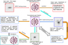 |
Fig. 2 Overview of the iterative training and TL process used in SAD-CNN. The first training stage begins with 1764 images of edge-on galaxies at z = 0, where the network learns to classify images based on the presence of faint features. The second stage introduces 3664 additional images of edge-on galaxies at different redshifts, improving classification performance on galaxies observed at various cosmological distances. Finally, the third stage applies TL to a dataset of 5264 images of galaxies with different disc inclinations, refining the model’s ability to generalise across varying orientations. Throughout the process, feedback is incorporated at each step, allowing for progressive learning and improved classification accuracy. |
4 Training process
Next, we discuss the process carried out to systematically and gradually train our CNN using the different samples and metrics discussed in Sect. 3. Our goal is to provide a more diverse and complex dataset at each training step, and thus we discuss the limitations behind this kind of method and provide potential ideas for future efforts.
4.1 Edge-on galaxies at redshift zero
For our initial training, we used the dataset from Group I. As mentioned in Section 3.4, this initial dataset covered 1764 (1050 originals) models of galaxies in an edge-on projection at z = 0.
For the training, validation, and test sets we randomly assign 80%, 10%, and 10% of the images, respectively. As previously discussed, the output of the CNN for each image is a value ranging from 0 to 1, which can be treated as the probability of the given images containing a LSBF. Values close to one indicate a high probability that a faint feature is present in the image, while values close to zero suggest a low probability.
The statistical summary of our first training step is presented in Table 1. In the initial phase, we consider outputs of the CNN above a threshold value of 0.5 as LSBF detections. With this threshold, our CNN achieved a precision of 0.86 in correctly identifying images without LSBF and 0.87 in detecting images with LSBF. Averaging, we obtained an overall precision, recall and F1-score of 0.87, indicating a well balanced performance assessment of our model. Following the initial training, we explored different threshold values to adjust the compromise between completeness and accuracy in stream detection. For example, a higher threshold value would produce a purer sample of true positives. However, this would result in a larger misidentification of images with streams as negative detections. To test this, we considered thresholds of 0.75 and 0.85. The results are also shown in Table 1. As expected, with these higher thresholds we recovered a purer true positive sample, but we misidentified a larger fraction of images with LSBFs as negative detection. This can be seen in the lower values of the Recall and F1-scores.
Figure 4 presents the confusion matrix obtained in this phase. The confusion matrix is a tabular representation that summarises the performance of a classification model, detailing metrics such as true positive rate (TP, equivalent to recall of detections), false positive rate (FP), true negative rate (TN, equivalent to recall of not detections), and false negative rate (FN). The left panel shows the matrix obtained with a 0.5 threshold value, where we obtain a reasonably high rate of TP and TN cases, both above 86%. The middle and right panels show the matrices obtained for threshold values of 0.75 and 0.85, respectively. As the threshold increased, the rates of FP and TP cases fell, while the rates of TN and FN cases increased. Note how the TP detection falls from 0.87 to 0.6 with the higher considered threshold. This exercise clearly shows that, while higher thresholds allow us to obtain a much cleaner sample of images with stellar streams (very low values of FP), this choice also results in a significant misclassification of images with streams as non-detections.
We explored in detail the distribution of classification model outputs and how they correlate with our visual classification. This is shown in Figure 5, where red and blue histograms show the output value distribution of TN and TP cases, respectively. Different panels correspond to the different thresholds considered. The histograms in this figure show a biased distribution of true cases towards 0 and 1, indicating that for a significant number of cases the CNN output aligns well with our visual classification. The FP and FN cases are shown in cyan and purple, respectively. Notably, false detections occur throughout the CNN output range, but are more frequent near the 0.5 threshold. Increasing the threshold significantly reduces the number of false positive detections (cyan histograms), in this particular case to 0, but increases false negative cases (purple histograms). Consequently, for very high precision values, several galaxies with visually identified LSBF are misclassified as non-detection cases.
We summarise the classification processes in Figure 6, where we show the normalised cumulative function of images with detected LSBF as a function of limiting SB magnitude, considering the threshold values previously introduced. The left, middle, and right panels correspond to precision thresholds of 0.5, 0.75 and 0.85, respectively. In each panel, the black and green lines show the identification obtained by SAD-CNN and our visual inspection, respectively. The blue line represents the cumulative functions obtained considering only TP (detections in agreement with our visual inspection). For the canonical threshold of 0.5 (left panel), the detection rate obtained by the CNN (black line), as a function of μlim, closely matches the cumulative function obtained from the visual inspection (green line). This could be due to a mix of true and false positive detections adding up to a similar cumulative function. However, as shown by the blue line, the cumulative function of true positive cases closely follows the CNN detection curve, highlighting the excellent performance of the model. This can also be seen by a very low fraction of false positive and negative detections at all μlim, shown by the purple and cyan lines. In the middle panel, by setting the threshold value at 0.75, we observe a decrease in the CNN detection rate (black line). However, it is now perfectly followed by the cumulative function of true positive cases, indicating a purer classification. Unfortunately, as previously discussed, this larger threshold is also associated with a significant increase in false negative cases (see purple line). Finally, in the right panel, we show the results obtained with a threshold equal to 0.85. Note that the purity of the CNN detection does not improve and, at the same time, the number of false negative cases significantly increases. As a result of this analysis, from here on, we work with a threshold of 0.5.
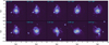 |
Fig. 3 Surface brightness maps of halo 12 from the Auriga simulation (AU12) illustrating the evolution of stellar streams under different disc plane rotations and snapshot times. The first row shows how the shape of the stream changes due to different viewing angles, while the second row highlights the temporal evolution of the streams. The maps have a surface brightness limit of |

SAD-CNN threshold levels.
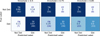 |
Fig. 4 Confusion matrices for the test set of galaxies at redshift zero, evaluated with threshold values of 0.5 (left), 0.75 (middle), and 0.85 (right). Each matrix corresponds to a subset of 105 test images. The top-left cell represents the true negative rate, the top-right cell the false positive rate, the bottom-left cell the false negative rate, and the bottom-right cell the true positive rate alongside the absolute counts (in parentheses). Further details on the performance metrics are provided in Table 1. |
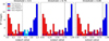 |
Fig. 5 Distribution of the prediction of SAD-CNN in the galaxies with edge-on projection at z=0 for different threshold values introduced by Figure 4. The threshold level is indicated with the dashed line. The red distribution shows the true negative cases. The purple distribution shows the false negative cases. The blue distribution shows the true positive cases. The cyan distribution shows the false positive cases by the SAD-CNN. |
4.2 Edge-on galaxies at different times
As described above in Section 3.4, Group II consists of images of galaxies with different ages up to a lookback time of ∼3 Gyr. These images capture different stages of late evolution, influenced by ongoing accretion events and merger histories. Figure 3 (bottom panels) shows an example, in which material from disrupted satellites gradually alters the structure of the halo. After separating 10% of the sample for the test set, we applied TL to retrain the SAD-CNN using the augmented training set of Group II consisting of 3664 images. This process aims to improve the model’s ability to classify halos whose structure and morphology evolve over time.
The results of this new training process are shown in Figure 7, where we compare the CNN performance on the Group II test set, before and after applying the TL procedure. The two top and two bottom panels correspond to the results obtained with previously trained model SAD-CNN (V-1 hereafter), and with the version obtained after TL (V-2 hereafter), respectively. We note that the V-1 was applied without retraining to a sample of galaxies at z > 0, since we seek to assess its generalisation capabilities. As shown in the top-left panel of Figure 7, the model V-1 performs poorly when applied to this sample of galaxies. After applying TL using the Group II training set, the new model V-2 shows a substantial improvement in classification performance, as seen in the bottom-left panel. In the right panels of Figure 7, we note that the number of FP is significantly reduced, improving the purity of the predicted positive sample, while there is a slight decrease in the TP rate, from 0.91 to 0.89, equivalent to three misclassified images. This behaviour is expected: the initial model V-1 tended to classify most faint features as detections, including cases where no real LSBF were present. This increased the TP rate, but also produced a high number of FP. After TL, the V-2 becomes more selective, correctly filtering out ambiguous cases where bright background features were previously mistaken as LSBF. Therefore, the small decrease in TP is a trade-off for a much greater reduction in FP, yielding a more balanced and robust classifier. We note that the F1-score increases from an average 0.85 in the V-1 to 0.90 in the V-2. Using the combined test sample from Groups I and II, both versions show consistent improvements: the average precision increase from 0.86 in V-1 to 0.90 and recall increase from 0.85 in V-1 to 0.90 in V-2.
The left and right panels of Figure 8 show the distribution of output values obtained from the V-1 and V-2 CNN, respectively. Here we focus on the ‘all z’ sample. We note that even though the distributions are similar, the V-2 has a more skewed distribution towards the maximum and minimum output values. This indicates that thanks to further training, CNN is more certain about its assessment. Table 2 summarises the results of this second training process.
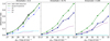 |
Fig. 6 Cumulative detection rate of LSBFs for all galaxies at z = 0. The black line represents the cumulative detection rate by SAD-CNN, while the green line corresponds to cumulative detection rate from visual inspection. The blue dashed line shows the cumulative fraction of only the true positive cases. The purple dashed line is the cumulative fraction rate produced with false negative cases, while the cyan dashed line corresponds to false positive detections. An over-detection trend is noticeable at SB limits fainter than ≈29 mag arcsec−2, which remains consistent across different threshold levels but is slightly shifted depending on the chosen threshold. |
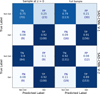 |
Fig. 7 Confusion matrices for SAD-CNN V-1 and V-2. The matrices on the left represent performance on the test sample at z > 0, while those on the right combine results from test samples. True negative (TN), false positive (FP), false negative (FN), and true positive (TP) rates are shown alongside the absolute counts (in parentheses). SAD-CNN V-2 demonstrates improved performance, particularly in reducing false positives (FP), as seen in the balanced predictions for both test scenarios. |
4.3 Most common false cases
We now explore the properties of the images that have been wrongly classified. Our goal is to compare the results obtained from the two versions of the SAD-CNN to improve the model. Figure 9 shows the distribution of false cases in the surface brightness versus the snapshot time space. The left panel shows that false cases in the SAD-CNN V-1 tend to be distributed about earlier snapshot lookback time (>1.5 Gyr), and mainly between 27 ≥ μlim ≥ 31 mag arcsec−2. In other words, even though the V-1 provides a reasonably good performance with the previously unseen dataset, most false cases are distributed at higher snapshot times. The right panel shows the distribution of false cases obtained with the V-2. We can clearly see that, after training CNN with images at higher snapshot times, the performance improves significantly. This only highlights the fact that the training set used in the V-1 was not sufficiently diverse.
In Figure 10, we show examples of these misclassified galaxies, in particular we show the examples of FP cases. Each image has a length of 300 kpc by side. The edge-on halos have discs of different sizes. The projected appearance of the discs varies due to intrinsic properties, with some showing more extended or asymmetric radial profiles (Grand et al. 2017). Most examples also exhibit bound satellite companions with signs of early tidal disruption. These complex morphologies challenge the classifier. In image B, multiple satellites interact with the host, producing a diffuse and irregular light distribution. While the larger number of images and TL in model V-2 help mitigate these effects, the difficulty increases further when varying disc inclinations, as discussed in the next section.
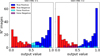 |
Fig. 8 Distribution of the prediction values of the first and second versions of the SAD-CNNs, shown in each panel, respectively. The threshold value used in these distributions is 0.5 and is indicated by the dashed line. Each panel includes values from the test sets of Groups I and II. The red distribution shows all true negative cases for each SAD-CNN version. The purple distribution shows the false negative cases. The blue distribution shows all detection by the SAD-CNN or the true positive. False positives are present by the cyan distribution. |
Comparison of SAD-CNN V-1 and V-2.
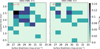 |
Fig. 9 Density distribution of all false cases (FP+FN). We present the density distribution for CNN V-1 and V-2 in the panels, respectively. The false cases are analysed as a function of surface brightness and snapshot lookback time. This arrangement allows for a detailed examination of the interplay between these parameters in the context of false cases. The total number of false cases (FCtot) is 32 and 18, respectively. This is normalised with the number of false cases and the number of the test sample (210 images). |
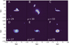 |
Fig. 10 Examples of FP cases in SAD-CNN. The first row illustrates various luminous structures such as satellite accretion or merging satellites that are misclassified as LSBFs taken from different Auriga halos at different snapshot lookback times. The second row displays FPs for halos at a 45° inclination. These models present prominent disc features, such as spiral arms, which were mistakenly classified as stellar streams. All models present the |

4.4 Galaxies with inclinations
The edge-on projection of disc galaxies represents the best configuration for detecting the stellar streams using surface brightness maps. However, galaxies in the Universe are randomly oriented. As shown in the previous section, structure arising from the stellar disc can be misidentified as debris from disrupting satellites. A similar situation takes place when prominent spiral arms arise in the images due to the disc inclination. To explore whether such inclined configurations significantly reduce the accuracy of our CNN, which was exclusively trained with models in edge-on configurations, we consider the images generated for Group III, described in Section 3.4. In this configuration, the mock images predominantly feature well-defined spiral structures, making them distinct from the earlier training sets.
In this new step, we incorporate 5264 new images using inclinations and rotations, applied to the initial sample with 1050 images at z = 0. As mentioned previously, the authors made a visual inspection to identify faint features. The results are summarised in the confusion matrix, shown in Figure 11. Here, the top panels show the result obtained from the V-2, whereas the second row shows the results after applying TL. We refer to this new model as SAD-CNN: V-3 (V-3 hereafter). The first three columns show the results obtained for images of where galactic discs are inclined by 15, 30, and 45 degrees, respectively. The last one shows the results for the complete sample. As expected, the top panel clearly shows that the precision values of our V-2 model rapidly declines as we increase the inclination of the sample. The increase in FP cases is significant, jumping from 24% in the i = 15 degrees sample to 70% in the i = 45 degrees sample. The overall results are shown in the upper right panel. Even though the recall remains at an average of 0.74 for all cases, the set of images with detected LSBF by the CNN V-2 would be strongly contaminated by FP cases. The results of the obtained metrics are reported in Table 3.
The results obtained after applying the TL, presented in the bottom panels of Figure 11, show a significant improvement.
Indeed, while we kept a high true positive detection rate, the fraction of false positives falls significantly at all inclinations. For example, at inclinations of 45 degrees, the FP rate shifts from 0.7 to 0.26 in V-3. The overall results, shown on the bottomright panel, indicate TN and TP rate values of 0.82% and 0.86%, respectively. With respect to the previous average recall values of 0.73 obtained with V-2 of CNN, the new average increase is at a value of 0.84.
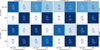 |
Fig. 11 Confusion matrices showing the results before and after the TL process of predictions of stellar streams in galaxies at different inclinations. The first and second rows correspond to the SAD-CNN results before and after TL, respectively. Each column represents a different inclination angle from Group III, with the last column presenting the results for the combined sample. The rows inside the matrix represent the true labels of the galaxies, meanwhile, the columns represent the predicted labels of the model. The matrix to the right in both cases presents the complete sample with all inclinations. |
Comparison SAD-CNN: V-2 & V-3.
4.5 Most common false cases
As previously done, we now explore the main characteristics of images associated with false cases. In Figure 12 we present the distribution of false cases at different surface brightness values as a function of the CNN output value. The results from the V-2 and V-3 models are shown in the first and second rows, respectively. The three columns indicate the distributions obtained at inclination angles of 15°, 30°, and 45°, respectively. The red dashed line shows the threshold value used to select positive and negative detections. As a result, the left half of these panels are associated with FN cases, whereas the right side with FP cases. All panels have been normalised by the total number of images in the test set. At low inclinations (15 degrees) a comparison between the V-2 and V-3 reveals no significant differences. The false cases are nearly uniformly distributed in SB limiting magnitude. However, as we increase the inclination the differences become significant. We can clearly see that the CNN V-2 model (top panels) starts to produce false positive detections with high output model values. This is particularly true for  mag arcsec−2. In other words, the model assigns high confidence scores to images that do not actually have LSBF. In Figure 10 we show examples of images that resulted in high confidence values as false positive detections by the CNN V-2 model. Notice that, as expected, all images present noticeable spiral arm patterns that are interpreted by the CNN as stellar streams. This limitation is reduced after applying TL, and as the models are further trained with inclined images. The bottom panels of Fig. 12 reveal that this overdensity of false positive cases, especially notorious at inclinations of 45 degrees in the V-2, is not present any longer. While the TL process applied to produce the V-3 model successfully reduced the number of false positives, especially at higher inclinations, a slight increase in FN was also observed across the test set. This trade-off illustrates a change in the model’s detection behaviour. As the selectivity increased, the model became more effective at rejecting spurious features, such as spiral arms or projection artefacts that were previously confused with LSBF, but at the cost of overlooking some genuine faint features. This result is interpreted as a gain in detection purity, although it comes with a modest loss in completeness. Therefore, it should be noted that the choice of model version should be based on the specific scientific objective, depending on whether the emphasis is on minimising false positives or maximising the detection rate of real LSBF structures.
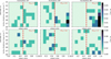 |
Fig. 12 Density distribution of all false cases in the prediction of SAD-CNN. The panels present the distribution of the output value and the surface brightness limit in the r-band for the different inclinations. The red lines separate the non-detection zone (threshold < 0.5) and the detection zone (threshold > 0.5). All panels have been normalised by the total number of images in the test set. |
5 SAD-CNN application
In order to test the accuracy of the final model, i.e. SAD-CNN V-3, we created three new datasets comprising images that had not been analysed during the previous training process at any stage.
In particular, for the first two tests, we considered input data images of the Auriga models at snapshots that had not previously been used in Group II (see Sect. 3.4). The redshifts for these tests are z = [0.06,0.09,0.11,0.14,0.17,0.2,0.23,0.26,0.29,0.33]. The first set consists of images with the galactic disc oriented edge-on. For each galaxy, we generated images at three randomly z from the previously list. Galaxies were twice randomly rotated about their symmetry axis. This set comprises 1260 images that have never been used in the learning process. As a second and more stringent test, we generated a set of galaxy images with randomly inclined galactic discs. The inclination angle, i, was randomly selected from a uniform distribution between 0 < i < 45 degrees. No perfectly edge-on galaxy was considered. As a result, we produce a new test set comprising a total of 1316 mock images, randomly oriented and at different times. This exercise allows us to quantify the performance of our different CNN models in a more realistic scenario. Finally, we performed a third test in which 200 random images of Milky Way-like galaxies from Illustris TNG50 simulation were considered. As described below, the orientation of each image was extracted as given in the cosmological box. This is the more challenging test for our SAD-CNN V-3 model as it considers galaxy models never seen neither during training nor validation.
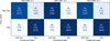 |
Fig. 13 Confusion matrices of the results of the different versions of the SAD-CNN. The tree panels present each version. The rows inside the matrix represent the true labels of the galaxies. Meanwhile, the columns represent the predicted labels of the model. |
5.1 Application in edge-on halos
This test focuses on images where galactic discs are oriented edge-on. We evaluated the three versions of SAD-CNN and compared their performance. The results of this test are summarised in Figure 13, where we show the resulting confusion matrices. The left, middle, and right panels show the performance of three versions of the SAD-CNN: V-1, V-2, and V-3, respectively. As expected for this image test set, all versions of the SAD-CNN exhibit a consistently high accuracy. The results were similar for all three versions of the model. They excel in identifying LSBFs in our mock images, with a true positive rate of ∼90%. On the other hand, the false positive cases reach a 16% of the images that were classified as non-detection by our visual classification. As previously discussed, typically these cases are associated with structures arising from the stellar disc or elongated satellites that can be observed in the mock images. The statistics of the three models provide an average precision, recall, and F1-score of ~0.88.
5.2 Application on inclined disc
In our second test, we classified a set of images in which the galactic discs are randomly inclined. As before, we generated the images considering random snapshots of the simulation that were not used during the training phase.
The top panels of Figure 14 show the confusion matrices obtained from this exercise. For clarity, here we only compare the results of the CNN V-1 and V-3 models. As expected, V-1 of the model can very efficiently identify images with LSBFs, with a true positive rate of 96% (top-left panel). However, it fails at classifying images with non-detections. Indeed, we obtained a false positive rate of 71%. This is mainly due to the inability of the V-1 of the model to deal with stellar disc substructures such as strong spiral arms. The bottom-left panel shows the density distribution of false cases as a function of SB limiting magnitude and the CNN output value. As seen in Sect. 4.4, the highest density peaks of false cases are associated with high CNN output values and SB magnitudes that go from ≥26 to 31 mag arcsec−2. This indicates that this version of the CNN produces false positive cases with a high certainty. The top-right panel of Fig. 14 shows the confusion matrix obtained after applying the V-3 of the model to the same test set. One can clearly appreciate a significant improvement with respect to V-1. We maintain a very high true positive rate of 86% and a reduced the false positive rate of 19%. The bottom-right panels show the distribution of false cases in the same space as before. We note that false cases with high CNN output values no longer exhibit a strong concentration. Instead, they now show a more uniform distribution across the output range. The improvement can also be seen in the values of the different metrics, listed in Table 4. We emphasise how the average precision, recall, and F1-score go from 0.4, 0.65, and 0.59 in V-1 to values of 0.8, 0.83, and 0.82 in V-3.
The results of this experiment not only demonstrate the accuracy of our CNN but also highlight how important it is to consider training datasets as diverse as possible. These datasets should incorporate not only images with different faint substructure morphologies but also other LSBFs associated with the host galaxy that could be confused by a CNN as debris from disrupted satellites.
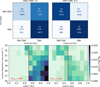 |
Fig. 14 Top panels: confusion matrices comparing the performance of SAD-CNN version 1 (left) and version 3 (right) on an independent test set of inclined galaxy halos, not used during training. The normalised fractions rates are shown together with the total number of predictions in each quadrant (in parenthesis). The rows inside the matrix represent the true labels of the galaxies, meanwhile, the columns represent the predicted labels of the model. Bottom panels: false classification density maps (FP + FN) as a function of CNN output value and surface brightness ( |


SAD-CNN application on inclined disc.
5.3 Application to TNG50
To evaluate the ability of SAD-CNN to generalise beyond the Auriga sample, we conducted an additional experiment using 200 Milky Way-like galaxies extracted from the IllustrisTNG50. TNG50 is a magnetohydrodynamical cosmological simulation that follows the formation and evolution of galaxies within a periodic box of 51.7 cMpc on a side, using the AREPO code with a moving-mesh hydrodynamics solver (see Nelson et al. 2019; Pillepich et al. 2019, for further details). TNG50 has a similar spatial and mass resolution to Auriga, with a baryonic mass resolution of 8.5 × 10⁴ M⊙ and gravitational softening lengths reaching 288 pc (physical) at z = 0. Unlike Auriga, which focuses on zoom-in simulations of relatively isolated Milky Way-mass halos, TNG50 includes a more statistically representative galaxy population, with a broader range of environments and formation histories. Also, the Auriga isolation criterion in this case is not necessarily represented. The galaxies used in this test were selected to be Milky Way analogues in stellar mass (2-10 × 1010 M⊙), providing a similar but independent test set to the Auriga sample. They provide a more diverse sample in terms of LSBF morphology and satellite orbital configurations. Crucially, these simulated galaxy sample was never seen by our SAD-CNN model, as they were not previously used either in training or validation. Their inclusion helps verify that the model trained on Auriga can generalise to diverse conditions and different assembly pathways.
For each galaxy, we generated an image with a randomly assigned surface brightness limit. In all cases we used the original random orientations, directly from the TNG50 box. Images were visually inspected and classified, finding that 73 images (36%) showed LSBF. In the remaining 127 images (64%) no LSBF were detected. The V-3 of our SAD-CNN model was applied directly to this test set, and the results are summarised in Figure 15. The top panel shows the resulting confusion matrix. The performance of our method is very good, and the results are consistent with those obtained on the final Auriga-based test sets. The classifier achieves an overall accuracy of approximately 86%, with a true positive rate of 90% and a true negative rate of 84%. the bottom panel on Figure 15 provides more information on the distribution of the 23 false classifications (FP + FN) in terms of the V-3 output and the limiting surface brightness. This is consistent with the fact that faint substructures, such as tidal features, are more difficult to discriminate from components of the disc or spiral arms, which can produce false classifications. Of the false cases, 74% are FP, while 26% are FN.
These results highlight that the model maintains strong predictive performance on unobserved data extracted from a different simulation, despite variations in halo properties and surface brightness. Furthermore, the modest number of false predictions in this diverse and challenging dataset further supports the robustness and applicability of methods such as SAD-CNN V-3 as a tool for the detection of LSBF.
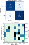 |
Fig. 15 Top panel: confusion matrix showing the performance of SAD-CNN V-3 on a random sample of 200 halos from the Illustris TNG50 simulation. Each halo image has a randomly assigned surface brightness distribution and orientation. The numbers in parenthesis indicate the absolute count of each classification result. Lower panel: density map of false cases (FP+FN) as a function of the V-3 output value and the surface brightness limit ( |

6 Discussion
The detection of LSBFs, such as stellar streams, shells, and plumes, in galaxy halos has attracted significant attention. These structures, which are remnants of the accretion of satellite galaxies, offer a unique window into a galaxy’s merger history and the processes shaping its stellar halo. Historically, such structures were detected by visual inspection of carefully reduced images in different photometric bands. Works such as Martínez-Delgado et al. (2010); Mouhcine et al. (2010); Atkinson et al. (2013); Monachesi et al. (2014); Morales et al. (2018); Mancillas et al. (2019); Martin et al. (2022); Martínez-Delgado et al. (2023); Miró-Carretero et al. (2023) provided the first relatively large datasets of deep observations of stellar halos where stellar streams could be detected through visual inspection. Several numerical analyses followed (Bullock & Johnston 2005; Shipp et al. 2018; Martin et al. 2022; Vera-Casanova et al. 2022; Miro-Carretero et al. 2025), placing constraints and providing predictions with respect to the information that could be extracted from the brightest detectable features. With the advent of deeper and larger observational surveys as well as more sophisticated numerical simulations, those working in this field have increasingly turned to automated methods to analyse the growing datasets. Among these methods, CNNs have emerged as powerful tools for image analysis and pattern recognition, particularly in astronomy. The stream automatic detection with convolutional neural networks (SAD-CNN) framework presented here contributes to this growing body of work by offering a method specifically optimised for detecting LSBFs. While SAD-CNN achieves a high accuracy in identifying LSBFs in simulated data, it is important to contextualise its performance within the broader landscape of similar approaches and the challenges inherent to such tasks.
A significant strength of SAD-CNN lies in its carefully designed training methodology. The model was progressively trained, starting with simplified scenarios (e.g. edge-on galaxies at z = 0) and later incorporating more complex configurations, such as varying galaxy inclinations and redshifts. This iterative approach, coupled with TL, allowed the model to adapt to increasingly challenging datasets and achieve precision and recall metrics above 84% in most scenarios. Additionally, the use of a well-balanced training dataset was critical for mitigating biases, ensuring that the CNN accurately distinguished between galaxies with and without LSBFs, at the surface brightness boundaries that have the strongest detection rates.
Our results not only show that the SAD-CNN approach is a viable way to efficiently and accurately detect LSBFs on large surveys, but they also clearly highlight that the diversity and quality of the training dataset remain critical. Misclassification, such as the false cases where spiral arms were identified as streams, highlights the importance of refining feature recognition in this type of model. Insufficient representation of complex morphologies or configurations can limit the power of the model. Extending the dataset to include interacting galaxies, noise effects, and other real-world complexities through additional TL steps would address some of these limitations and further improve the robustness of the model. However, we tested our SAD-CNN on a randomly sampled dataset with Milky Way-like mass galaxies. We chose 200 halos with a completely random orientation from the Illustris TNG50 simulation (Pillepich et al. 2019). From there, a random brightness limit was selected between 27 and 32 mag arcsec−2 to evaluate the performance. We tested the ability of the model to detect LSBFs in simulated images with considerable confidence in order to determine that this tool can be used for research. In this case, the accuracy is still above 84% , which is a strong indicator that the neural network is correctly focused on the recognition of faint features.
When upcoming large-scale surveys, such as those conducted by the Vera C. Rubin Observatory and EUCLID (Ivezic et al. 2019; Euclid Collaboration: Aussel et al. 2025), begin to deliver unprecedented volumes of deep imaging data, the role of automated tools such as SAD-CNN will become increasingly critical. These tools not only accelerate the detection process but also enable statistical analyses of LSBFs across diverse galaxy populations. However, ensuring the reliability of these methods when applied to observational data will require careful calibration and validation, particularly to account for observational artefacts, noise, and varying spatial resolutions. In addition, a diverse and large training dataset will be required to further optimise the efficiency and accuracy of such models. As a next step, we plan to apply SAD-CNN to a much larger extracted simulated observational dataset and additionally include a variation in the resolution of the simulated image with different pixel sizes depending on the targeted redshift.
The combination of CNN with complementary techniques, such as Bayesian inference or clustering algorithms, could provide a more comprehensive framework for studying LSBFs or other features (Euclid Collaboration: Busillo et al. 2025). This integration would enable more robust estimates of such physical parameters as faint features, age, mass, and orbital history, which are critical for constraining galaxy formation models.
Although the results presented here demonstrate the robustness of the SAD-CNN model in detecting faint features under a wide range of simulated conditions, future work should include tests with real observational data. These data will pose new challenges, such as the presence of foreground and background contamination, noise, incomplete sky coverage, and the effects of dust extinction. These factors can significantly alter the visual appearance of LSBFs and may affect the performance of the network. However, the flexibility of our approach and the modular structure of SAD-CNN provide a solid foundation for adapting and retraining the model to manage such observational complexities. In summary, SAD-CNN represents an important step forward in automating the detection of LSBFs in galaxy halos. While its performance is promising, its effectiveness should be evaluated alongside other methods to fully appreciate its contributions and limitations. Future work should focus on diversifying training datasets, incorporating additional simulation and observational data, and exploring hybrid approaches to address the challenges of feature misclassification.
Data availability
The data underlying this article will be shared on reasonable request to the corresponding author.
Acknowledgements
AVC and FAG acknowledge support from Agencia Nacional de Investigación y Desarrollo (ANID) Fondo Nacional de Desarrollo Científico y Tecnológico (FONDECYT) Regular 1211370. FAG gratefully acknowledges support by the ANID BASAL project FB210003. D.P. acknowledges financial support from ANID through FONDECYT Postdoctrorado Project 3230379. RB is supported by the SNSF through the Ambizione Grant PZ00P2-223532. FvdV is supported by a Royal Society University Research Fellowship (URF R1 191703 and URF R 241005). We also thank the anonymous referee for his thoughtful and respectful comments, which have greatly improved the quality and clarity of this manuscript.
References
- Amorisco, N. C. 2017, MNRAS, 464, 2882 [Google Scholar]
- Atkinson, A. M., Abraham, R. G., & Ferguson, A. M. N. 2013, ApJ, 765, 28 [Google Scholar]
- Baxter, D. C., Cooper, M. C., & Fillingham, S. P. 2021, MNRAS, 503, 1636 [Google Scholar]
- Belokurov, V., Zucker, D. B., Evans, N. W., et al. 2006, ApJ, 642, L137 [Google Scholar]
- Belokurov, V., Erkal, D., Evans, N. W., Koposov, S. E., & Deason, A. J. 2018, MNRAS, 478, 611 [Google Scholar]
- Bickley, R. W., Bottrell, C., Hani, M. H., et al. 2021, MNRAS, 504, 372 [NASA ADS] [CrossRef] [Google Scholar]
- Bílek, M., Duc, P.-A., Cuillandre, J.-C., et al. 2020, MNRAS, 498, 2138 [Google Scholar]
- Bonaca, A., & Price-Whelan, A. M. 2025, New A Rev., 100, 101713 [Google Scholar]
- Bruzual, G., & Charlot, S. 2003, MNRAS, 344, 1000 [NASA ADS] [CrossRef] [Google Scholar]
- Bullock, J. S., & Johnston, K. V. 2005, ApJ, 635, 931 [Google Scholar]
- Chollet, F. 2016, arXive-prints [arXiv:1610.02357] [Google Scholar]
- Conselice, C. J., Bershady, M. A., & Jangren, A. 2000, ApJ, 529, 886 [NASA ADS] [CrossRef] [Google Scholar]
- Cooper, A. P., Cole, S., Frenk, C. S., et al. 2010, MNRAS, 406, 744 [Google Scholar]
- Cooper, A. P., D’Souza, R., Kauffmann, G., et al. 2013, MNRAS, 434, 3348 [Google Scholar]
- Deng, J., Dong, W., Socher, R., et al. 2009, in 2009 IEEE Conference on Computer Vision and Pattern Recognition, 248 [Google Scholar]
- Duc, P.-A. 2017, in IAU Symposium, 321, Formation and Evolution of Galaxy Outskirts, eds. A. Gil de Paz, J. H. Knapen, & J. C. Lee, 180 [Google Scholar]
- Dumoulin, V., & Visin, F. 2016, arXiv e-prints [arXiv:1603.07285] [Google Scholar]
- Erkal, D., & Belokurov, V. 2015, MNRAS, 454, 3542 [NASA ADS] [CrossRef] [Google Scholar]
- Euclid Collaboration (Aussel, H., et al.) 2025, A&A, submitted [arXiv:2503.15302] [Google Scholar]
- Euclid Collaboration (Busillo, V., et al.) 2025, A&A, submitted [arXiv:2503.15329] [Google Scholar]
- Farias, H., Ortiz, D., Damke, G., Jaque Arancibia, M., & Solar, M. 2020, Astron. Comput., 33, 100420 [NASA ADS] [CrossRef] [Google Scholar]
- Fattahi, A., Deason, A. J., Frenk, C. S., et al. 2020, MNRAS, 497, 4459 [NASA ADS] [CrossRef] [Google Scholar]
- Fliri, J., & Trujillo, I. 2016, MNRAS, 456, 1359 [Google Scholar]
- Fontirroig, V., Gómez, F. A., Jaque Arancibia, M., Dolfi, A., & Monsalves, N. 2025, A&A, 699, A118 [NASA ADS] [CrossRef] [EDP Sciences] [Google Scholar]
- Gaia Collaboration (Brown, A. G. A., et al.) 2018, A&A, 616, A1 [NASA ADS] [CrossRef] [EDP Sciences] [Google Scholar]
- Gatys, L. A., Ecker, A. S., Bethge, M., Hertzmann, A., & Shechtman, E. 2016, arXiv e-prints [arXiv:1611.07865] [Google Scholar]
- Gómez, F. A., & Helmi, A. 2010, MNRAS, 401, 2285 [Google Scholar]
- Gonzalez-Jara, J., Tissera, P. B., Monachesi, A., et al. 2025, A&A, 693, A282 [NASA ADS] [CrossRef] [EDP Sciences] [Google Scholar]
- Gordon, A. J., Ferguson, A. M. N., & Mann, R. G. 2024, MNRAS, 534, 1459 [Google Scholar]
- Grand, R. J. J., Gómez, F. A., Marinacci, F., et al. 2017, MNRAS, 467, 179 [NASA ADS] [Google Scholar]
- Grand, R. J. J., Fragkoudi, F., Gómez, F. A., et al. 2024, MNRAS, 532, 1814 [NASA ADS] [CrossRef] [Google Scholar]
- Helmi, A. 2008, A&A Rev., 15, 145 [NASA ADS] [CrossRef] [Google Scholar]
- Helmi, A. 2020, ARA&A, 58, 205 [Google Scholar]
- Helmi, A., & White, S. D. M. 1999, MNRAS, 307, 495 [CrossRef] [Google Scholar]
- Helmi, A., White, S. D. M., de Zeeuw, P. T., & Zhao, H. 1999, Nature, 402, 53 [Google Scholar]
- Helmi, A., Navarro, J. F., Meza, A., Steinmetz, M., & Eke, V. R. 2003a, ApJ, 592, L25 [Google Scholar]
- Helmi, A., White, S. D. M., & Springel, V. 2003b, MNRAS, 339, 834 [NASA ADS] [CrossRef] [Google Scholar]
- Helmi, A., Cooper, A. P., White, S. D. M., et al. 2011, ApJ, 733, L7 [Google Scholar]
- Hibbard, J. E., & Mihos, J. C. 1995, AJ, 110, 140 [Google Scholar]
- Hood, C. E., Kannappan, S. J., Stark, D. V., et al. 2018, ApJ, 857, 144 [NASA ADS] [CrossRef] [Google Scholar]
- Hopkins, P. F., Wetzel, A., Keres, D., et al. 2018, MNRAS, 480, 800 [NASA ADS] [CrossRef] [Google Scholar]
- Ibata, R. A., Gilmore, G., & Irwin, M. J. 1994, Nature, 370, 194 [Google Scholar]
- Ibata, R., Malhan, K., Martin, N., et al. 2021, ApJ, 914, 123 [NASA ADS] [CrossRef] [Google Scholar]
- Iman, M., Rasheed, K., & Arabnia, H. R. 2023, Technologies, 11, 40 [Google Scholar]
- Ivezic, Z., Kahn, S. M., Tyson, J. A., et al. 2019, ApJ, 873, 111 [NASA ADS] [CrossRef] [Google Scholar]
- Janowiecki, S., Mihos, J. C., Harding, P., et al. 2010, ApJ, 715, 972 [Google Scholar]
- Ji, I., Peirani, S., & Yi, S. K. 2014, A&A, 566, A97 [NASA ADS] [CrossRef] [EDP Sciences] [Google Scholar]
- Johnston, K. V., Hernquist, L., & Bolte, M. 1996, ApJ, 465, 278 [NASA ADS] [CrossRef] [Google Scholar]
- Johnston, K. V., Bullock, J. S., Sharma, S., et al. 2008, ApJ, 689, 936 [Google Scholar]
- Kado-Fong, E., Greene, J. E., Hendel, D., et al. 2018, ApJ, 866, 103 [NASA ADS] [CrossRef] [Google Scholar]
- Kado-Fong, E., Sanderson, R. E., Greene, J. E., et al. 2022, ApJ, 931, 152 [Google Scholar]
- Keras Team 2022, Keras. [Online]. Available: https://keras.io/api/callbacks/early_stopping/ [Accessed: 13-Jan-2022] [Google Scholar]
- Kingma, D. P., & Ba, J. 2014, arXiv e-prints [arXiv:1412.6980] [Google Scholar]
- LeCun, Y., Bengio, Y., & Hinton, G. 2015, Nature, 521, 436 [Google Scholar]
- Li, Y.-S., & Helmi, A. 2008, MNRAS, 385, 1365 [NASA ADS] [CrossRef] [Google Scholar]
- Li, T. S., Koposov, S. E., Erkal, D., et al. 2021, ApJ, 911, 149 [CrossRef] [Google Scholar]
- Lotz, J. M., Jonsson, P., Cox, T. J., & Primack, J. R. 2008, MNRAS, 391, 1137 [Google Scholar]
- Majewski, S. R., Siegel, M. H., Kunkel, W. E., et al. 1999, AJ, 118, 1709 [Google Scholar]
- Malhan, K., Ibata, R. A., & Martin, N. F. 2018, MNRAS, 481, 3442 [Google Scholar]
- Mancillas, B., Duc, P.-A., Combes, F., et al. 2019, A&A, 632, A122 [NASA ADS] [CrossRef] [EDP Sciences] [Google Scholar]
- Martin, G., Bazkiaei, A. E., Spavone, M., et al. 2022, MNRAS, 513, 1459 [NASA ADS] [CrossRef] [Google Scholar]
- Martínez-Delgado, D., Gabany, R. J., Crawford, K., et al. 2010, AJ, 140, 962 [Google Scholar]
- Martínez-Delgado, D., Cooper, A. P., Román, J., et al. 2023, A&A, 671, A141 [NASA ADS] [CrossRef] [EDP Sciences] [Google Scholar]
- McConnachie, A. W., Irwin, M. J., Ibata, R. A., et al. 2009, Nature, 461, 66 [Google Scholar]
- Meza, A., Navarro, J. F., Abadi, M. G., & Steinmetz, M. 2005, MNRAS, 359, 93 [CrossRef] [Google Scholar]
- Miró-Carretero, J., Martínez-Delgado, D., Farràs-Aloy, S., et al. 2023, A&A, 669, L13 [NASA ADS] [CrossRef] [EDP Sciences] [Google Scholar]
- Miro-Carretero, J., Gomez-Flechoso, M. A., Martinez-Delgado, D., et al. 2025, A&A, 700, A176 [Google Scholar]
- Monachesi, A., Bell, E. F., Radburn-Smith, D. J., et al. 2014, ApJ, 780, 179 [Google Scholar]
- Monachesi, A., Gómez, F. A., Grand, R. J. J., et al. 2016, MNRAS, 459, L46 [NASA ADS] [CrossRef] [Google Scholar]
- Monachesi, A., Gómez, F. A., Grand , R. J. J., et al. 2019, MNRAS, 485, 2589 [NASA ADS] [CrossRef] [Google Scholar]
- Morales, G., Martínez-Delgado, D., Grebel, E. K., et al. 2018, A&A, 614, A143 [NASA ADS] [CrossRef] [EDP Sciences] [Google Scholar]
- Mouhcine, M., Harris, W. E., Ibata, R., & Rejkuba, M. 2010, MNRAS, 404, 1157 [NASA ADS] [Google Scholar]
- Nelson, D., Springel, V., Pillepich, A., et al. 2019, MNRAS, 490, 3234 [Google Scholar]
- Pakmor, R., Springel, V., Bauer, A., et al. 2016, MNRAS, 455, 1134 [Google Scholar]
- Perez, L., & Wang, J. 2017, arXiv e-prints [arXiv:1712.04621] [Google Scholar]
- Pillepich, A., Madau, P., & Mayer, L. 2015, ApJ, 799, 184 [Google Scholar]
- Pillepich, A., Nelson, D., Springel, V., et al. 2019, MNRAS, 490, 3196 [Google Scholar]
- Planck Collaboration XVI. 2014, A&A, 571, A16 [NASA ADS] [CrossRef] [EDP Sciences] [Google Scholar]
- Pu, S.-Y., Cooper, A. P., Grand, R. J. J., Gómez, F. A., & Monachesi, A. 2025, ApJ, 980, 63 [Google Scholar]
- Quinn, P. J. 1984, ApJ, 279, 596 [Google Scholar]
- Riley, A. H., Shipp, N., Simpson, C. M., et al. 2025, MNRAS, 542, 2443 [Google Scholar]
- Rutherford, T. H., van de Sande, J., Croom, S. M., et al. 2024, MNRAS, 529, 810 [NASA ADS] [CrossRef] [Google Scholar]
- Sánchez-Sáez, P., Lira, H., Martí, L., et al. 2021, AJ, 162, 206 [CrossRef] [Google Scholar]
- Schaye, J., Crain, R. A., Bower, R. G., et al. 2015, MNRAS, 446, 521 [Google Scholar]
- Searle, L., & Zinn, R. 1978, ApJ, 225, 357 [Google Scholar]
- Shipp, N., Drlica-Wagner, A., Balbinot, E., et al. 2018, ApJ, 862, 114 [Google Scholar]
- Shipp, N., Panithanpaisal, N., Necib, L., et al. 2023, ApJ, 949, 44 [NASA ADS] [CrossRef] [Google Scholar]
- Shipp, N., Riley, A. H., Simpson, C. M., et al. 2025, MNRAS, 542, 1109 [Google Scholar]
- Simpson, C. M., Grand, R. J. J., Gómez, F. A., et al. 2018, MNRAS, 478, 548 [CrossRef] [Google Scholar]
- Smercina, A., Bell, E. F., Price, P. A., et al. 2023, ApJ, 949, L37 [Google Scholar]
- Sola, E., Duc, P.-A., Richards, F., et al. 2022, A&A, 662, A124 [NASA ADS] [CrossRef] [EDP Sciences] [Google Scholar]
- Springel, V. 2010, MNRAS, 401, 791 [Google Scholar]
- Springel, V., & Hernquist, L. 2003, MNRAS, 339, 289 [Google Scholar]
- Tau, E. A., Monachesi, A., Gomez, F. A., et al. 2025, A&A, 699, A93 [NASA ADS] [CrossRef] [EDP Sciences] [Google Scholar]
- Tissera, P. B., Scannapieco, C., Beers, T. C., & Carollo, D. 2013, MNRAS, 432, 3391 [NASA ADS] [CrossRef] [Google Scholar]
- Tissera, P. B., Beers, T. C., Carollo, D., & Scannapieco, C. 2014, MNRAS, 439, 3128 [NASA ADS] [CrossRef] [Google Scholar]
- Tumlinson, J. 2010, ApJ, 708, 1398 [CrossRef] [Google Scholar]
- Valenzuela, L. M., & Remus, R.-S. 2024, A&A, 686, A182 [NASA ADS] [CrossRef] [EDP Sciences] [Google Scholar]
- Vera-Casanova, A., Gómez, F. A., Monachesi, A., et al. 2022, MNRAS, 514, 4898 [NASA ADS] [CrossRef] [Google Scholar]
- Villalobos, Á., & Helmi, A. 2008, MNRAS, 391, 1806 [Google Scholar]
- Vogelsberger, M., Genel, S., Sijacki, D., et al. 2013, MNRAS, 436, 3031 [Google Scholar]
- Walder, M., Erkal, D., Collins, M., & Martinez-Delgado, D. 2025, ApJ, 994, 36 [Google Scholar]
- Walmsley, M., Ferguson, A. M. N., Mann, R. G., & Lintott, C. J. 2019, MNRAS, 483, 2968 [NASA ADS] [CrossRef] [Google Scholar]
- White, S. D. M., & Frenk, C. S. 1991, ApJ, 379, 52 [Google Scholar]
- White, S. D. M., & Rees, M. J. 1978, MNRAS, 183, 341 [Google Scholar]
Learning curves are shown in the Appendix.
Appendix A Learning curves
The learning curves presented in the appendix illustrate the training progress of the SAD-CNN model by tracking key performance metrics over multiple epochs. These curves typically show how the loss function and accuracy (or other evaluation metrics) evolve for both the training and validation datasets.
By analysing these curves, we assess whether early stopping is needed to prevent overfitting, if additional training epochs could improve performance, or if adjustments in hyperparameters (e.g. learning rate) are necessary.
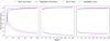 |
Fig. A.1 Learning curves for the different versions of the SAD-CNN training process, panels correspond V-1, V-2, and V-3 respectively. The plot illustrates the model’s performance during training and validation for each network version. The x-axis represents the number of epochs, while the y-axis indicates the loss function values. The curves demonstrate how the model’s error decreases over time for both the training (red lines) and validation (blue lines) sets. |
All Tables
All Figures
|
Fig. 1 Example of data augmentation applied to the test sample of images with and without stellar streams. The left panel shows the original test sample distribution at z = 0, where images are unevenly distributed across SB limits ( |
| In the text | |
|
Fig. 2 Overview of the iterative training and TL process used in SAD-CNN. The first training stage begins with 1764 images of edge-on galaxies at z = 0, where the network learns to classify images based on the presence of faint features. The second stage introduces 3664 additional images of edge-on galaxies at different redshifts, improving classification performance on galaxies observed at various cosmological distances. Finally, the third stage applies TL to a dataset of 5264 images of galaxies with different disc inclinations, refining the model’s ability to generalise across varying orientations. Throughout the process, feedback is incorporated at each step, allowing for progressive learning and improved classification accuracy. |
| In the text | |
|
Fig. 3 Surface brightness maps of halo 12 from the Auriga simulation (AU12) illustrating the evolution of stellar streams under different disc plane rotations and snapshot times. The first row shows how the shape of the stream changes due to different viewing angles, while the second row highlights the temporal evolution of the streams. The maps have a surface brightness limit of |
| In the text | |
|
Fig. 4 Confusion matrices for the test set of galaxies at redshift zero, evaluated with threshold values of 0.5 (left), 0.75 (middle), and 0.85 (right). Each matrix corresponds to a subset of 105 test images. The top-left cell represents the true negative rate, the top-right cell the false positive rate, the bottom-left cell the false negative rate, and the bottom-right cell the true positive rate alongside the absolute counts (in parentheses). Further details on the performance metrics are provided in Table 1. |
| In the text | |
|
Fig. 5 Distribution of the prediction of SAD-CNN in the galaxies with edge-on projection at z=0 for different threshold values introduced by Figure 4. The threshold level is indicated with the dashed line. The red distribution shows the true negative cases. The purple distribution shows the false negative cases. The blue distribution shows the true positive cases. The cyan distribution shows the false positive cases by the SAD-CNN. |
| In the text | |
|
Fig. 6 Cumulative detection rate of LSBFs for all galaxies at z = 0. The black line represents the cumulative detection rate by SAD-CNN, while the green line corresponds to cumulative detection rate from visual inspection. The blue dashed line shows the cumulative fraction of only the true positive cases. The purple dashed line is the cumulative fraction rate produced with false negative cases, while the cyan dashed line corresponds to false positive detections. An over-detection trend is noticeable at SB limits fainter than ≈29 mag arcsec−2, which remains consistent across different threshold levels but is slightly shifted depending on the chosen threshold. |
| In the text | |
|
Fig. 7 Confusion matrices for SAD-CNN V-1 and V-2. The matrices on the left represent performance on the test sample at z > 0, while those on the right combine results from test samples. True negative (TN), false positive (FP), false negative (FN), and true positive (TP) rates are shown alongside the absolute counts (in parentheses). SAD-CNN V-2 demonstrates improved performance, particularly in reducing false positives (FP), as seen in the balanced predictions for both test scenarios. |
| In the text | |
|
Fig. 8 Distribution of the prediction values of the first and second versions of the SAD-CNNs, shown in each panel, respectively. The threshold value used in these distributions is 0.5 and is indicated by the dashed line. Each panel includes values from the test sets of Groups I and II. The red distribution shows all true negative cases for each SAD-CNN version. The purple distribution shows the false negative cases. The blue distribution shows all detection by the SAD-CNN or the true positive. False positives are present by the cyan distribution. |
| In the text | |
|
Fig. 9 Density distribution of all false cases (FP+FN). We present the density distribution for CNN V-1 and V-2 in the panels, respectively. The false cases are analysed as a function of surface brightness and snapshot lookback time. This arrangement allows for a detailed examination of the interplay between these parameters in the context of false cases. The total number of false cases (FCtot) is 32 and 18, respectively. This is normalised with the number of false cases and the number of the test sample (210 images). |
| In the text | |
|
Fig. 10 Examples of FP cases in SAD-CNN. The first row illustrates various luminous structures such as satellite accretion or merging satellites that are misclassified as LSBFs taken from different Auriga halos at different snapshot lookback times. The second row displays FPs for halos at a 45° inclination. These models present prominent disc features, such as spiral arms, which were mistakenly classified as stellar streams. All models present the |
| In the text | |
|
Fig. 11 Confusion matrices showing the results before and after the TL process of predictions of stellar streams in galaxies at different inclinations. The first and second rows correspond to the SAD-CNN results before and after TL, respectively. Each column represents a different inclination angle from Group III, with the last column presenting the results for the combined sample. The rows inside the matrix represent the true labels of the galaxies, meanwhile, the columns represent the predicted labels of the model. The matrix to the right in both cases presents the complete sample with all inclinations. |
| In the text | |
|
Fig. 12 Density distribution of all false cases in the prediction of SAD-CNN. The panels present the distribution of the output value and the surface brightness limit in the r-band for the different inclinations. The red lines separate the non-detection zone (threshold < 0.5) and the detection zone (threshold > 0.5). All panels have been normalised by the total number of images in the test set. |
| In the text | |
|
Fig. 13 Confusion matrices of the results of the different versions of the SAD-CNN. The tree panels present each version. The rows inside the matrix represent the true labels of the galaxies. Meanwhile, the columns represent the predicted labels of the model. |
| In the text | |
|
Fig. 14 Top panels: confusion matrices comparing the performance of SAD-CNN version 1 (left) and version 3 (right) on an independent test set of inclined galaxy halos, not used during training. The normalised fractions rates are shown together with the total number of predictions in each quadrant (in parenthesis). The rows inside the matrix represent the true labels of the galaxies, meanwhile, the columns represent the predicted labels of the model. Bottom panels: false classification density maps (FP + FN) as a function of CNN output value and surface brightness ( |
| In the text | |
|
Fig. 15 Top panel: confusion matrix showing the performance of SAD-CNN V-3 on a random sample of 200 halos from the Illustris TNG50 simulation. Each halo image has a randomly assigned surface brightness distribution and orientation. The numbers in parenthesis indicate the absolute count of each classification result. Lower panel: density map of false cases (FP+FN) as a function of the V-3 output value and the surface brightness limit ( |
| In the text | |
|
Fig. A.1 Learning curves for the different versions of the SAD-CNN training process, panels correspond V-1, V-2, and V-3 respectively. The plot illustrates the model’s performance during training and validation for each network version. The x-axis represents the number of epochs, while the y-axis indicates the loss function values. The curves demonstrate how the model’s error decreases over time for both the training (red lines) and validation (blue lines) sets. |
| In the text | |
Current usage metrics show cumulative count of Article Views (full-text article views including HTML views, PDF and ePub downloads, according to the available data) and Abstracts Views on Vision4Press platform.
Data correspond to usage on the plateform after 2015. The current usage metrics is available 48-96 hours after online publication and is updated daily on week days.
Initial download of the metrics may take a while.