| Issue |
A&A
Volume 704, December 2025
|
|
|---|---|---|
| Article Number | A18 | |
| Number of page(s) | 30 | |
| Section | Stellar atmospheres | |
| DOI | https://doi.org/10.1051/0004-6361/202554900 | |
| Published online | 02 December 2025 | |
High-angular-resolution ALMA imaging of the inhomogeneous dynamical atmosphere of the asymptotic giant branch star W Hya
SiO, H2O, SO2, SO, HCN, AlO, AlOH, TiO, TiO2, and OH lines
1
Instituto de Astrofísica, Departamento de Física y Astronomía, Facultad de Ciencias Exactas, Universidad Andrés Bello,
Fernández Concha 700, Las Condes,
Santiago,
Chile
2
Department of Physics and Astronomy, Uppsala University,
Box 516,
751 20
Uppsala,
Sweden
3
Max-Planck-Institut für Radioastronomie,
Auf dem Hügel 69,
53121
Bonn,
Germany
★ Corresponding author: This email address is being protected from spambots. You need JavaScript enabled to view it.
Received:
31
March
2025
Accepted:
9
September
2025
Abstract
Aims. We present high-angular-resolution imaging of the asymptotic giant branch star W Hya with the Atacama Large Millimeter/submillimeter Array (ALMA) to probe the dynamics and chemistry in the atmosphere and inner wind.
Methods. W Hya was observed with the longest baselines of ALMA at 250–268 GHz with an angular resolution of ~17×20 mas.
Results. ALMA’s high angular resolution allowed us to resolve the stellar disk of W Hya along with clumpy, irregularly shaped emission extending to ~100 mas. This emission includes a plume in the north-northwest, a tail in the south-southwest, and the extended atmosphere elongated in the east-northeast-west-southwest direction, with semimajor and semiminor axes of ~70 and 40 mas (~3.4 and 1.9 R⋆), respectively. We identified 57 lines, which include SiO, H2O, SO2, SO, HCN, AlO, AlOH, TiO, TiO2, OH, and some of their isotopologues, with about half of them being in vibrationally excited states. The molecular line images show spatially inhomogeneous molecular formation. Our ALMA data taken at phase 0.53 (minimum light) indicate global, accelerating infall within ~75 mas (3.6 R⋆) but also outflow at up to ~10 km s−1 in deeper layers. While 38 of the detected lines appear in absorption against the continuum stellar disk as expected, we detect nonthermal emission on top of the continuum over the stellar disk in 19 lines, including SiO, H2O, SO2, and AlO. The emission of the SiO, AlO, TiO, TiO2, SO, and SO2 lines coincides well with the clumpy dust cloud distribution obtained from contemporaneous visible polarimetric imaging in addition to H2O reported in our previous work. This lends support to the idea that SiO, H2O, and AlO are directly involved in grain nucleation. The overlap of SO/SO2 (possibly also TiO/TiO2) with the dust clouds suggests the formation of these molecules and dust behind shocks induced by pulsation and/or convection. We detect HCN emission close to the star, down to ~30 mas (~1.4 R⋆), which is consistent with shock-induced chemistry.
Key words: stars: AGB and post-AGB / circumstellar matter / stars: imaging / stars: mass-loss / stars: individual: W Hya / radio lines: stars
© The Authors 2025
 Open Access article, published by EDP Sciences, under the terms of the Creative Commons Attribution License (https://creativecommons.org/licenses/by/4.0), which permits unrestricted use, distribution, and reproduction in any medium, provided the original work is properly cited.
This article is published in open access under the Subscribe to Open model. This email address is being protected from spambots. You need JavaScript enabled to view it. to support open access publication.
1 Introduction
Low- and intermediate-mass stars experience significant mass loss at the asymptotic giant branch (AGB), which plays an important role not only in stellar evolution but also in the chemical evolution of galaxies, because nuclear-processed material is returned to the interstellar space via mass loss. It is often postulated that large-amplitude pulsation levitates the material, which leads to density enhancement in the cool, upper atmosphere, where dust can form. The radiation pressure on the dust grains can then drive the mass loss (Höfner & Olofsson 2018). Furthermore, the recent 3D models of the dynamical atmosphere of AGB stars show that dust formation can occur in low-temperature regions caused by convective inhomogeneities in density and temperature (Freytag & Höfner 2023).
To clarify the long-standing problem of the mass loss from AGB stars, it is indispensable to probe the region within a few R⋆, where the dust forms and the wind accelerates. The advance in high-angular observation techniques has made it possible to spatially resolve this key region. Infrared long-baseline interferometric imaging has revealed inhomogeneous structures over the stellar disk and in the atmosphere of AGB stars with milliarcsecond angular resolution (e.g., Wittkowski et al. 2017; Paladini et al. 2018; Ohnaka et al. 2019; Drevon et al. 2022; Planquart et al. 2024). For example, the imaging of the AGB star R Dor in the 2.3 μm CO lines with the AMBER instrument at the Very Large Telescope Interferometer (VLTI) shows the irregularly shaped, clumpy atmosphere extending to ~2 R⋆ (Ohnaka et al. 2019). They also obtained 2D velocity-field maps over the surface and atmosphere at different atmospheric heights and revealed strong outward acceleration between ~1.5 and 1.8 R⋆. These inhomogeneities in the atmosphere may be the seed of the clumpy cloud formation, which has been detected in some AGB stars (Ireland et al. 2005; Norris et al. 2012; Khouri et al. 2016, 2018; Ohnaka et al. 2016, 2017; Adam & Ohnaka 2019).
The Atacama Large Millimeter/submillimeter Array (ALMA) also provides us with the spatial resolution needed to resolve the atmosphere and the innermost circumstellar environment of nearby cool evolved stars. Takigawa et al. (2017) imaged the atmosphere of the AGB star W Hya in the AlO line at 344 GHz with ALMA. Vlemmings et al. (2017) obtained a continuum image of W Hya from the same data, which shows a hot spot over the stellar disk. The ATOMIUM Large Program observed 17 oxygen-rich AGB stars and red supergiants (RSGs) between ~214 and 270 GHz at high angular resolutions to study the gas dynamics and chemical properties in the stellar winds (Decin et al. 2020; Gottlieb et al. 2022; Wallström et al. 2024). Khouri et al. (2024) presented a detailed analysis of the kinematical structure of the extended atmosphere and the innermost circumstellar envelope of R Dor, taking advantage of the ALMA data in the CO lines that spatially resolved the stellar disk. More recently, Vlemmings et al. (2024) imaged convective cells over the surface of R Dor with ALMA and their time variations within a month. Velilla-Prieto et al. (2023) showed the formation of different molecular species in spatially distinct regions of the clumpy atmosphere of the dusty carbon star IRC+10216. Asaki et al. (2023) imaged the compact HCN maser emission from the carbon star R Lep with an angular resolution of down to 5 mas.
In this paper, we present ALMA observations of the AGB star W Hya at spatial resolutions of 17–20 mas at 250–268 GHz. (Ohnaka et al. 2024; hereafter Paper I) reported the results on the 268 GHz continuum and two vibrationally excited H2O lines from the same data. Here, we present the complete results on all the detected lines. In Sect. 2, we provide an overview of the basic properties of W Hya derived in the literature. Our ALMA observations and data reduction are described in Sect. 3. We describe the observational results and interpretation of the data of the detected spectral lines in Sect. 4. A discussion on the molecule-dust chemistry and dynamics in the atmosphere and the inner wind is presented in Sect. 5, followed by concluding remarks in Sect. 6.
2 Basic properties of W Hya
The oxygen-rich AGB star W Hya is one of the AGB stars closest to the Sun, and therefore, it has been extensively studied from the visible to the infrared to the radio (e.g., Zhao-Geisler et al. 2011; Khouri et al. 2015 and references therein). While it is classified as a semi-regular variable of type a (SRa), it shows a clear periodicity with 389 days (Uttenthaler et al. 2011, see also discussion in Nowotny et al. 2010 for the classification of W Hya).
The distances of W Hya measured with different methods show some discrepancies. Vlemmings et al. (2003) measured a distance of ![Mathematical equation: $\[98_{-18}^{+30}\]$](/articles/aa/full_html/2025/12/aa54900-25/aa54900-25-eq1.png) pc based on the OH maser parallax. They interpret the errors as due to the variations in the stellar atmosphere, for example, caused by stellar pulsation. Knapp et al. (2003) obtained a smaller distance of
pc based on the OH maser parallax. They interpret the errors as due to the variations in the stellar atmosphere, for example, caused by stellar pulsation. Knapp et al. (2003) obtained a smaller distance of ![Mathematical equation: $\[78_{-5.6}^{+6.5}\]$](/articles/aa/full_html/2025/12/aa54900-25/aa54900-25-eq2.png) pc from the reprocessed Hipparcos parallax. They also derived a period-luminosity relation based on the reprocessed Hipparcos parallax for a sample of semiregular variables (W Hya is one of them). Recently Andriantsaralaza et al. (2022) derived a distance of
pc from the reprocessed Hipparcos parallax. They also derived a period-luminosity relation based on the reprocessed Hipparcos parallax for a sample of semiregular variables (W Hya is one of them). Recently Andriantsaralaza et al. (2022) derived a distance of ![Mathematical equation: $\[87_{-9}^{+11}\]$](/articles/aa/full_html/2025/12/aa54900-25/aa54900-25-eq3.png) pc based on this period-luminosity relation for semi-regular variables1. On the other hand, van Leeuwen (2007) obtained a parallax of 9.59 ± 1.12 mas based on another reprocessing of the Hipparcos data, which translates into a distance of
pc based on this period-luminosity relation for semi-regular variables1. On the other hand, van Leeuwen (2007) obtained a parallax of 9.59 ± 1.12 mas based on another reprocessing of the Hipparcos data, which translates into a distance of ![Mathematical equation: $\[104_{-11}^{+14}\]$](/articles/aa/full_html/2025/12/aa54900-25/aa54900-25-eq4.png) pc, in agreement with the result of Vlemmings et al. (2003). In the present work, we adopted the 98 pc from Vlemmings et al. (2003) because their method with the high-angular-resolution measurements allowed them to separate the parallax and residual motions due to the variations in the stellar atmosphere.
pc, in agreement with the result of Vlemmings et al. (2003). In the present work, we adopted the 98 pc from Vlemmings et al. (2003) because their method with the high-angular-resolution measurements allowed them to separate the parallax and residual motions due to the variations in the stellar atmosphere.
The wind terminal velocity has been determined from various observations primarily in the far-infrared and radio. For example, Khouri et al. (2014a) derived 7.5 km s−1 by the model fitting to the CO line profiles, while Hoai et al. (2022) obtained, based on the analysis of ALMA data, a lower value of 5 km s−1, which is outside the parameter range of the model fitting of Khouri et al. (2014a). Hoai et al. (2022) also pointed out that the CO masers reported by Vlemmings et al. (2021) appear at a blueshifted velocity of ~5.5 km s−1. In the present work, we adopted the wind terminal velocity of 5 km s−1. As for the systemic velocity, Khouri et al. (2014a) derived 40.4 km s−1 in the local standard of rest (LSR), which is in agreement with the previous studies (see references therein). However, they note that the high-J 13CO lines are better fit with a systemic velocity of 39.6 km s−1. Vlemmings et al. (2017) also derived a similar, lower value of 39.2 km s−1. The systemic velocity of 40.4 km s−1 was adopted in our analysis, because it agrees with the values derived from various observations.
We adopted 41.4 mas as the star’s angular diameter (i.e., 20.7 mas as the star’s angular radius R⋆), as described in Paper I. Combined with the distance of 98 pc, this translates into a linear radius of 3 × 1013 cm (430 R⊙).
As described in Sect. 3, our ALMA observations took place at phase 0.53. Ohnaka et al. (2017) derived the bolometric flux of 1.69 × 10⁻⁸ W m−2 at approximately the same phase of 0.54, which corresponds to a bolometric luminosity of 5070 L⊙ at the adopted distance of 98 pc. Combining the bolometric flux and the angular diameter of 41.4 mas results in an effective temperature of 2330 K.
3 Observations and data reduction
Our ALMA observations took place between June 7, 2019, and June 8, 2019, from 22:52 to 04:42 (UTC) in four consecutive execution blocks (EBs) in Cycle 6 with the C43-10 configuration of the 12-m array (Program ID: 2018.1.01239.S, P.I.: K. Ohnaka). The variability phase of W Hya at the time of our ALMA observations was 0.53 at minimum light. Each EB consists of 53–55 target scans with a scan length up to 54.4 s. The on-source time of each EB is about 45 min, and the total on-source time of the project is about 3 hours. The quasar J1337–1257 was observed as the bandpass and absolute flux calibrator, J1342–2900 as the phase-referencing calibrator, and J1351–2912 as the check source.
The observations were carried out under very good atmospheric conditions with a precipitable water vapor (PWV) of about 0.55 mm. W Hya was observed from an elevation of ~59° through its transit at ~85° until ~44°. This resulted in a broad and nonoverlapping hour angle range, and hence a good uv coverage. The shortest and longest baselines are 83.1 m and 16.2 km, respectively, which results in an angular resolution of 16–20 mas and a largest recoverable scale of 190 mas at the observed frequencies.
As listed in Table 1, the spectral setups consist of nine spectral windows (spws) centered at 250.7, 251.8, 252.5, 253.7, 265.9, 266.9, 267.2, 267.7, and 268.2 GHz. The bandwidth of the first seven windows is 468.75 MHz, while that of the windows at 267.7 and 268.2 GHz is 937.50 MHz. The four highest-frequency windows (spws 6–9) partially overlap together. The channel width in each spectral window is 488.3 kHz. The velocity resolution of 1.1–1.2 km s−1 corresponds to twice the spectral channel width with the Hanning smoothing at the correlator.
The visibility data were calibrated with the Common Astronomy Software Applications CASA (Casa Team 2022), version 5.6.1–8, following the standard steps of the ALMA Cycle 7 pipeline. Among 44 antennas in the array, DA54 and DA61 were completely flagged due to bad amplitudes. After the pipeline calibration, we self-calibrated the data and manually reconstructed the images. We first identified spectral channels containing line emission or absorption from an initial set of image cubes and produced the continuum visibility data from the line-free channels. The continuum images of W Hya were reconstructed, which provided initial models for self-calibration, which was done in two iterations. The first iteration was for phase alone with the solution interval being the scan length (≲54 s). The second iteration was for both the amplitude and phase using the entire EB (~45 min) as the solution interval.
The continuum and spectral line images of W Hya were reconstructed from the self-calibrated visibility data. We adopted a pixel scale of 3 mas and the robust weighting with a robustness parameter of 0.5 in the CASA task tclean. For the vibrationally excited HCN line (v2 = 11e, J = 3–2) at 265.853 GHz (Sect. 4.12) and AlOH (J = 8–7) line at 251.795 GHz (Sect. 4.13), we reconstructed the images with the natural weighting to enhance the weak extended emission. We also imaged the continuum data in each spectral window using the multifrequency synthesis (MFS) method. Because the millimeter continuum of W Hya is spatially resolved, we deconvolved the images with the multi-scale algorithm (Cornwell 2008) for size scales of 1 (point sources), 5, and 15 pixels and with a small-scale bias parameter of 0.7. The typical RMS noise in the continuum MFS images is ~40 μJy/beam. The restoring beams for the continuum images are about 19 × 17 mas in the lower sideband (spws 1–4) and 18 × 16 mas in the upper sideband (spws 5–9) as listed in Table 1.
Except for HCN v = 0, J = 3–2 at 265.886 GHz and SO v = 0, NJ = 65−54 at 251.826 GHz, the emission of most spectral lines is confined within a radius of ![Mathematical equation: $\[{\sim}0^{\prime\prime}_\cdot2\]$](/articles/aa/full_html/2025/12/aa54900-25/aa54900-25-eq5.png) from the center of the continuum emission. The RMS noise in the spectral line cubes is typically ~0.5–0.6 mJy/beam over the channel width of 488 kHz (Table 1). As discussed in Sect. 4.7, spw 4 covers the 29SiO v = 2 J = 6–5 line, which exhibits strong maser emission in W Hya. Due to the dynamic range limit, the RMS noise is much higher in the channels containing the strongest emission, up to 2.7 mJy/beam. The maximum imaging dynamic range is close to 6800.
from the center of the continuum emission. The RMS noise in the spectral line cubes is typically ~0.5–0.6 mJy/beam over the channel width of 488 kHz (Table 1). As discussed in Sect. 4.7, spw 4 covers the 29SiO v = 2 J = 6–5 line, which exhibits strong maser emission in W Hya. Due to the dynamic range limit, the RMS noise is much higher in the channels containing the strongest emission, up to 2.7 mJy/beam. The maximum imaging dynamic range is close to 6800.
In order to determine the position of the stellar disk center, we fit the visibility data at the line-free spectral channels in each spectral window before self-calibration with a uniform ellipse using uvmultifit (Martí-Vidal et al. 2014). The continuum disk center averaged over the different spectral windows is (α, δ) = (13:49:01.92528, −28:22:04.69895) in the International Celestial Reference System (ICRS). The images presented in this paper are centered at this disk center position.
We identified the spectral line detections mainly using the Splatalogue service2, the Cologne Database for Molecular Spectroscopy3 (CDMS, Endres et al. 2016; Müller et al. 2001, 2005), the Jet Propulsion Laboratory (JPL) catalog4 (Pickett et al. 1998), and the HITRAN database5 (Gordon et al. 2022). Table 2 lists the 57 molecular lines identified in the present work, which include 29SiO, 30SiO, Si17O, H2O, SO2, 34SO2, 33SO2, SO, AlO, AlOH, HCN, TiO, 49TiO, 50TiO, TiO2, and OH.
Figure 1 gives an overview of the continuum-subtracted images of the different molecular lines at the systemic velocity, which cover most of the identified species including two H2O lines reported in Paper I (the channel maps and/or integrated intensity maps of all the detected lines will be presented below and in Appendices on Zenodo https://doi.org/10.5281/zenodo.17118092). ALMA’s high angular resolution allows us to resolve the stellar disk and highly inhomogeneous atmosphere and innermost circumstellar envelope. The different molecular lines show distinct morphology, indicating differences in their formation and excitation.
Spectral windows (spws) of our ALMA observations of W Hya.
4 Results
4.1 Continuum
In Paper I, we presented the continuum image restored with a beam of 18 × 16 mas in the 268.2 GHz spectral window (spw 9), which can be fit with a uniform elliptical disk with a major and minor axis of 59.1 ± 0.3 mas and 57.7 ± 0.2 mas with a position angle of 16 ± 23°. The continuum images obtained in other spectral windows are similar to the one at 268.2 GHz as shown in Fig. A.1. The aforementioned uniform elliptical disk fitting to the continuum data in other spectral windows results in major and minor axes of 58–60 mas, as found at 268.2 GHz. In the present work, we use the geometrical mean of the major and minor axis of 59.3 mas derived in Paper I as the millimeter continuum angular diameter (i.e., 29.6 mas as the continuum angular radius Rcont).
Table 1 lists the flux densities integrated over the continuum images in nine spectral windows. The flux densities are in broad agreement with the measurement by Dehaes et al. (2007), who obtained 280.0 ± 17.2 mJy at 250 GHz with a full width at half maximum (FWHM) bandwidth of 90 GHz in May 2003 (phase 0.65). As Fig. 2 shows, the continuum flux measurements can be well fit with a power law, Fv ∝ v2.08±0.03. This is close to the power-law index of 1.86 expected from the radio-photosphere model, where the opacity source is mainly optically thick free-free emission (Reid & Menten 1997, 2007; Matthews et al. 2015).
The millimeter continuum angular size at 250–268 GHz is 1.4 times larger than the star’s angular diameter of 41.4 mas adopted in the present work (Sect. 2). Our continuum angular size is in broad agreement with the (69 ± 10) × (46 ± 7) mas obtained at 43 GHz by Reid & Menten (2007), but it is larger than the 56.5 × 51.0 mas obtained at 338 GHz by Vlemmings et al. (2017) at a variability phase of ~0.3. Given that the free-free opacity decreases with the frequency, the difference in the continuum angular size can be explained if the continuum at 251–268 GHz forms at layers slightly farther away from the star than that at 338 GHz. However, it is also possible that the phase dependence of the angular size is responsible for the observed difference in the continuum angular size as discussed by Matthews et al. (2015) and recently modeled by Bojnordi Arbab et al. (2024).
All continuum images obtained at 250.7–268.2 GHz show a slight offset of the intensity peak to the northwest (NW) by 5–7 mas (0.2–0.3 R⋆) from the center of the stellar disk obtained by the aforementioned uniform elliptical disk fitting, but the asymmetry in the intensity is 1% at most, as described for the 268.2 GHz continuum image in Paper I. Although the contemporaneous visible polarimetric imaging reveals clumpy dust cloud formation within ~2 R⋆ (Paper I), the asymmetry in the millimeter continuum images cannot be attributed to a dust clump for the following reason. Ohnaka et al. (2017) derived a dust optical depth of 0.8 at 0.55 μm from the visible polarimetric imaging of W Hya at minimum light. This translates into a dust optical depth at 268 GHz (![Mathematical equation: $\[\tau_{\mathrm{mm}}^{\text {dust}}\]$](/articles/aa/full_html/2025/12/aa54900-25/aa54900-25-eq6.png) ) of 10−7, if we adopt the optical constants of forsterite (Mg2SiO4) from Jäger et al. (2003) and a grain size of 0.1 μm. Approximating the stellar continuum intensity I⋆ with the blackbody radiation at 2150 K (see below), the dust thermal emission Idust is estimated as
) of 10−7, if we adopt the optical constants of forsterite (Mg2SiO4) from Jäger et al. (2003) and a grain size of 0.1 μm. Approximating the stellar continuum intensity I⋆ with the blackbody radiation at 2150 K (see below), the dust thermal emission Idust is estimated as ![Mathematical equation: $\[I_{\star} e^{-\tau_{\mathrm{mm}}^{\mathrm{dust}}}+B_{\nu}(T_{\mathrm{dust}})(1-e^{-\tau_{\mathrm{mm}}^{\mathrm{dust}}})\]$](/articles/aa/full_html/2025/12/aa54900-25/aa54900-25-eq7.png) . Assuming a condensation temperature of 1500 K for Tdust, the difference between the stellar continuum intensity and dust emission intensity is ~10−7 of the stellar continuum intensity, too small to account for the observed contrast of 1% of the asymmetry.
. Assuming a condensation temperature of 1500 K for Tdust, the difference between the stellar continuum intensity and dust emission intensity is ~10−7 of the stellar continuum intensity, too small to account for the observed contrast of 1% of the asymmetry.
The observed smooth continuum images is in marked contrast to the detection of a hot spot over the stellar disk of W Hya in the 338 GHz continuum reported by Vlemmings et al. (2017), although our spatial resolution of 20×17 mas is comparable to their restoring beam size of 17 mas. They derived a brightness temperature as high as >5.3 × 10⁴ K. The presence of hot gas may be temporarily variable, given that the ALMA observations of Vlemmings et al. (2017) took place in December 2015 (~3.5 years ≈ 3.3 pulsation cycles before our observations). However, Hoai et al. (2022), imaging the 338 GHz continuum from the same dataset, did not reproduce such a hot spot. Detailed investigation of the imaging and model fitting of the 338 GHz continuum image would be necessary, which is, however, beyond the scope of the present paper.
The uniform elliptical disk fitting in nine spectral windows results in brightness temperatures of 2130–2170 K over the millimeter continuum stellar disk. Assuming that the continuum is formed by the optically thick free-free emission, the derived brightness temperatures correspond to the gas temperature in the millimeter-continuum-forming layers. Given the effective temperature of 2330 K (Sect. 2), the gas temperature falls off only slightly from the photosphere to the millimeter continuum-forming layers at ~1.4 R⋆. Vlemmings et al. (2017) derived a brightness temperature of 2495 ± 255 K averaged over the entire stellar disk observed at 338 GHz at phase 0.3, while their continuum image (their Fig. 1) shows that the brightness temperature over the stellar disk outside the hot spot is lower, 1800–2300 K. Reid & Menten (2007) imaged W Hya in the 43 GHz continuum at phase 0.25 and derived a brightness temperature of 2380 ± 550 K. The radio photosphere model of Reid & Menten (1997) predicts the brightness temperature to increase with the frequency. However, the large uncertainties, inhomogeneities over the stellar disk as well as the phase dependence of the atmosphere make it difficult to compare with the prediction of the radio photosphere model. Contemporaneous observations with comparable angular resolutions will be useful to address this point.
Molecular lines identified in our ALMA observations of W Hya in Band 6.
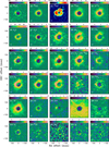 |
Fig. 1 Continuum-subtracted maps of W Hya observed at the systemic velocity in the different molecular lines presented in the main text. The images of two H2O lines (#6 and #7) are from Paper I. The color scale shown above each panel corresponds to mJy/beam except for #3, where it is given in Jy/beam. The black circles represent the ellipse fit to the continuum image. The identification number of each line in Table 2 is shown in the upper left corner. The restoring beam size is shown in the lower left corner of each panel. North is up, and east is to the left. |
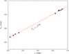 |
Fig. 2 Continuum spectrum of W Hya at 250–268 GHz. The black dots represent the observed continuum fluxes, while the solid red line represents a power-law fit with Fv ∝ v2.08. The horizontal bars show the bandwidth of the spectral windows, not errors. |
4.2 29SiO v = 3, J = 6–5 at 251.930 GHz
Figure 3 shows the continuum-subtracted channel maps obtained for the 29SiO line (v = 3, J = 6–5) at 251.930 GHz with a restoring beam size of 21 × 18 mas. In each panel, the velocity in the LSR as well as the relative velocity with respect to the systemic velocity Vrel = VLSR − Vsys is shown. The images show compact emission extending to a radius of ~40 mas (~1.3 Rcont = 1.9 R⋆), which means that the 29SiO line probes the region close to the star because of its high upper level energy of 5266 K. Furthermore, thanks to the spatial resolution of ~20 mas and the large angular size of W Hya, we can see absorption over the stellar disk, which is expected because the gas temperature is generally lower than the continuum brightness temperature, and it decreases with the radial distance. Along the line of sight to the stellar disk, the cooler layers of 29SiO line formation absorb the background continuum, resulting in an absorption spectrum. The redshifted and blueshifted velocities of the absorption indicate infalling and outflowing motions, respectively.
Our ALMA images reveal that the absorption over the stellar disk is inhomogeneous. The images obtained at velocities from Vrel = 1.5 to 7.5 km s−1 show prominent absorption in the southwest (SW) region of the stellar disk, revealing an infalling gas clump or cell. On the other hand, the images obtained at Vrel = −9 to ~0 km s−1 show that absorption is particularly deep in the northeast (NE)–east (E)–southeast (SE) regions.
To see the variation of the absorption over the stellar disk, we extracted spatially resolved spectra from the data cube without the continuum subtraction at five different positions over the stellar disk: at the center of the fitted elliptical disk and four positions with a radial offset of 15 mas (0.5 Rcont) at position angles of −15°, 75°, 165°, and 255°, which we refer to as position 0, 1, 2, 3, and 4, respectively, as labeled in Fig. 4a. The four position angles were selected to probe the plume, tail, and extended, elongated atmosphere, which will be described in the next subsections.
Figure 4 (left column, black lines) reveals that the spectra of 29SiO obtained at all five positions show broad absorption extending approximately from Vrel = −16 to 10 km s−1, which indicates the presence of outflowing and infalling layers along the line of sight over the stellar disk. We present a simple model to explain the observed data in Sect. 4.5. If the current mass of W Hya is assumed to be 1 M⊙ based on the results of Khouri et al. (2014b) and Danilovich et al. (2017), the escape velocity at 40 mas (1.9 R⋆ = 3.9 au at the distance of 98 pc) is 21 km s−1, which is higher than the outflow velocity seen in the 29SiO absorption line. Therefore, the material within ~2 R⋆ is still gravitationally bound if only marginally. The observed velocity range of the 29SiO line is in broad agreement – albeit somewhat smaller – with the velocities from −20 to 20 km s−1 seen in the CO v = 1 J = 3–2 line toward W Hya (Vlemmings et al. 2017), given the difference in the upper level energy and possible time variations. The broad line profile is also observed in the first-overtone (v = 2–0) SiO lines near 4 μm for a sample of Mira-type and semi-regular variables (Lebzelter et al. 2001). They show that the 4 μm SiO lines are broad, approximately covering from −20 to 20 km s−1 with respect to the systemic velocity, comparable to the velocity width of the millimeter 29SiO line.
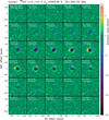 |
Fig. 3 Continuum-subtracted channel maps of W Hya observed in the 29SiO v = 3 J = 6–5 line at 251.930123 GHz. The black circles represent the ellipse fit to the continuum image. In the upper left corner of each panel, the LSR velocity and the relative velocity Vrel = VLSR − Vsys, Vsys = 40.4 km s−1 are shown. The restoring beam size is shown in the lower left corner of each panel. North is up, and east is to the left. |
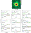 |
Fig. 4 Spatially resolved spectra of four SiO lines detected in our ALMA observations. (a) Continuum-subtracted intensity map of the Si 17O line (v = 0, J = 6–5) integrated from Vrel = −10 to 10 km s−1. The crosses and numbers represent the positions where the spatially resolved spectra shown in panels b–p were derived. (b–f) Spatially resolved spectra observed at five positions over the stellar disk. The black, red, green, and blue lines represent the spectra of the 29SiO v = 3 J = 6–5, 30SiO v = 2 J = 6–5, 30SiO v = 1 J = 6–5, and Si17O v = 0 J = 6–5 lines, respectively. The spectra were obtained from the data cube with the continuum emission. (g–k) SiO spectra obtained at positions 5–8 at a radial distance of 50 mas from the stellar disk center. These spectra were extracted from the continuum-subtracted data cube. The spectra measured at the disk center are shown in panel g to facilitate comparison between the absorption and emission spectra. (l–p) SiO spectra obtained at positions 9–12 at a radial distance of 90 mas from the stellar disk center, shown in the same manner as in panels g–k. |
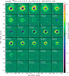 |
Fig. 5 Continuum-subtracted channel maps of W Hya obtained in the 30SiO v = 2 J = 6–5 line at 250.727751 GHz, shown in the same manner as Fig. 3. The maps at Vrel ≤ −10.5 km s−1 are severely affected by the Si17O line at 250.745 GHz (presented in Fig. 9). |
4.3 30SiO v = 2, J = 6–5 at 250.728 GHz
Figure 5 shows the continuum-subtracted channel maps of the 30SiO line (v = 2, J = 6–5) at 250.728 GHz. The images at velocities more blueshifted than Vrel ≈ −10.5 km s−1 are severely contaminated by the adjacent Si17O line at 250.745 GHz (see Sect. 4.6). The images obtained near the systemic velocity show emission elongated in the east-northeast (ENE)-west-southwest (WSW) direction with a semimajor and semiminor axis of ~45 mas (1.5 Rcont = 2.2 R⋆) and ~40 mas (1.3 Rcont = 1.9 R⋆), respectively. The elongated emission is similar to that seen in the 29SiO line (v = 3 J= 6–5) presented in Fig. 3. However, the emission is slightly more extended and more prominent, because the upper level energy of 3520 K of the 30SiO (v = 2) line is lower than that of the 29SiO (v = 3) line (5266 K).
The channel maps obtained at Vrel = −9 to −6 km s−1 show prominent blueshifted absorption in the northern region of the stellar disk. Strong absorption appears in the SE region of the stellar disk at Vrel = −4.5 to 0 km s−1. These features are seen in the channel maps of the 29SiO line described above. On the other hand, the channel maps obtained at Vrel = 1.5 to 9 km s−1 show that the bright ring-like emission extends inward over the stellar disk, different from that of the 29SiO line. The "leak" of the emission off the stellar limb into the stellar disk can occur due to the finite beam size (e.g, Wong et al. 2016). However, the channel maps at some other velocity channels (e.g., Vrel = −3.0 and −1.5 km s−1) do not show emission over the stellar disk in spite of the strong emission just outside the stellar limb, particularly in the east. Therefore, the emission detected over the stellar disk at the redshifted velocities cannot be attributed to such a leak due to the finite beam size.
The spatially resolved spectra (Fig. 4, left column, red lines) show that the blue part of the absorption of the 30SiO line between Vrel = −10 and 0 km s−1 is nearly identical to that of the 29SiO line (black lines in the figure). As will be discussed in the next subsections, the spectra of the 30SiO v = 1 J = 6–5 line (and Si17O v = 0 J = 6–5 line to some extent) in this blueshifted velocity range are identical. This suggests that the blue part of these lines is optically thick, corresponding to the same brightness temperature. In an optically thick case, this means that these lines originate from the gas at the same kinetic temperature at the same radial range.
However, the red part shows noticeably shallower absorption or even emission at some velocities due to the aforementioned emission over the stellar disk. For the same reason, at position 4, the deepest absorption at the redshifted velocity of ~5 km s−1 seen in the spectrum of the 29SiO line is also absent. The emission over the stellar disk manifests itself as a bump at Vrel = 3 to 10 km s−1 in the spectrum at position 2 (PA = 75°) and also at position 1 (PA = −15°) to a lesser extent. The redshifted emission over the stellar disk may seem to indicate the presence of gas hotter than the 2100–2200 K of the continuum-forming layer. However, if we assume that different molecular species have the same kinetic temperature and they are in local thermodynamical equilibrium (LTE), such hot gas would give rise to emission over the stellar disk in the 29SiO v = 3 line as well as the 30SiO v = 1 line (Sect. 4.2), which is not observed. If a line forms in non-LTE, its excitation is determined not only by the collision but also by the radiative pumping, and therefore, the line can appear in absorption or emission. In Sect. 4.6, we present the interpretation that the redshifted emission over the stellar disk is of the nonthermal origin – suprathermal (excitation temperature > kinetic temperature) or maser action (excitation temperature < 0).
4.4 30SiO v= 1, J = 6–5 at 252.471 GHz
The continuum-subtracted channel maps of the 30SiO v = 1 J = 6–5 line at 252.471 GHz, shown in Fig. 6, reveal a complex outer atmosphere extending out to a radius of ~100 mas (i.e., ~3.3 Rcont = 4.8 R⋆). It is much more prominent and more extended than in the 29SiO v = 3 and 30SiO v = 2 lines, because the upper level energy of 1790 K is lower than those of the two SiO lines presented above. Three prominent features can be recognized in Fig. 6: a plume in the north-northwest (NNW), a tail in the south-southeast (SSE), and the extended atmosphere elongated in the ENE–WSW direction.
We extracted spatially resolved spectra at the same five positions over the stellar disk as in the case of the 29SiO and 30SiO lines. Spectra were also extracted off the limb of the star, at angular radii of 50 mas (1.7 Rcont = 2.4 R⋆) and 90 mas (3 Rcont = 4.3 R⋆), at the same four position angles of −15°, 75°, 165°, and 255° (Fig. 4, middle and right columns). The spectra obtained at PA = −15° and 165° correspond to the plume and tail, respectively, while those obtained at PA = 75° and 255° probe the extended atmosphere.
The spectra extracted over the stellar disk (positions 0 to 4), plotted in Fig. 4 (left column, green lines), show blueshifted absorption extending to Vrel ≈ −15 km s−1, which is nearly identical to that of the lines of 29SiO v = 3 and 30SiO v = 2, because these SiO lines are optically thick in their blue part as explained in Sect. 4.3. On the other hand, the spectra of the 30SiO v = 1 line exhibit very deep redshifted absorption with the strongest absorption at Vrel = 3–7 km s−1, extending to Vrel ≈ + 15 km s−1 except for position 4 at PA = 225°. This deep redshifted absorption is not seen in other SiO lines described above.
In order to estimate where the redshifted deep absorption originates, we examined the p-V diagram extracted in the direction at PA = 45°−225° with a slit width of 5 mas from the 30SiO v = 1 data. We selected this direction because the redshifted absorption appears to be the strongest in the NE (PA ≈ 45°) and the weakest in the southwest (SW, PA ≈ 225°). The resulting p-V diagram is shown in Fig. 7. Assuming that the most prominent emission and the deepest absorption on the NE side trace a coherent kinematic structure in the form of a partial spherical shell, we may derive the extent of different shells by tracing various patterns in the p-V diagram. First, the deepest absorption over the stellar disk and the brightest emission off the stellar limb on the NE side can be fit with an infall velocity of 7 km s−1 and a radius of 50 mas (1.7 Rcont = 2.4 R⋆) as shown with the red line in Fig. 7. Second, the most redshifted absorption over the stellar disk on the NE side can be traced by the infall velocity of up to 13 km s−1 and a radius of 42 mas (1.4 Rcont = 2.0 R⋆) as shown with the light blue line. Third, the most extended emission on the NE side near the systemic velocity can be fit with an infall velocity of 2 km s−1 and a radius of 75 mas (2.5 Rcont = 3.6 R⋆) as shown with the pink line. Fourth, the emission off the limb of the star on the SW side can be fit with a partial shell with a radius of 45 mas (1.5 Rcont = 2.2 R⋆) radially expanding or infalling at 12 km s−1 as show by the blue line.
This interpretation means an accelerating infall on the NE side (PA = 45°) from ~2 km s−1 at 3.6 R⋆ to ~7 km s−1 at 2.4 R⋆ and then to ~13 km s−1 at 2.0 R⋆. The strong redshifted absorption observed over the stellar disk suggests the infall from PA = −15° to ~165°. Also, the infalling material seen off the limb of the stellar disk can lead to redshifted self-absorption due to colder material on the near side. The emission spectrum of the 30SiO v = 1 line extracted on the NE side at 50 mas ≈ 1.7 Rcont (Fig. 4i, position 6, green line) indeed shows that the red part is weaker or suppressed compared to the blue part. The same trend is also seen in the 30SiO v = 2 (red line) and Si17O v = 0 (blue line in Fig. 4i, described in Sect. 4.6 below) lines. In light of these signatures of self-absorption in the emission spectra, it is possible that self-absorption contributes to the absorption spectra of the 30SiO v = 1, 30SiO v = 2, and Si17O v = 0 lines over the stellar disk. In the case of the 29SiO v = 3 line, self-absorption cannot be confirmed, because while the blue part is very weak at position 6 (Fig. 4i, black line), the emission off the stellar limb is compact, and no emission is detected at other positions.
The fitting on the SW side in the p-V diagram in Fig. 7 does not allow us to distinguish between infall and expansion. However, the emission spectrum of the 30SiO v = 1 line at position 8 (Fig. 4k, green line) shows that the red part is weak or suppressed – the same signature of self-absorption due to the infalling material on the near side. In addition, the vibrationally excited H2O line at 268 GHz (v2 = 2, 65,2−74,3) reported in Paper I shows mostly infall in the SW region at ~2 Rcont = 2.9 R⋆. Therefore, it is more plausible that the material in the SW region is also infalling.
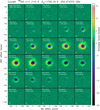 |
Fig. 6 Continuum-subtracted channel maps of W Hya obtained in the 30SiO v = 1 J = 6–5 line at 252.471372 GHz, shown in the same manner as Fig. 3. |
4.5 Modeling of the 30SiO v = 1 and 29SiO v = 3 lines
We constructed a spherical model in LTE to examine whether the above picture can account for the observed spectra of the 30SiO v = 1 line as well as the 29SiO v = 3 line. We assumed LTE primarily for simplicity, because full non-LTE radiative transfer modeling is beyond the scope of this paper. Neither of the two lines shows nonthermal (suprathermal or maser) emission over the stellar disk, which would be evidence of non-LTE. We refrain from modeling the 30SiO v = 2 (Sect. 4.3) and Si17O v = 0 lines (below in Sect. 4.6) in the present work, because they exhibit nonthermal emission over the stellar disk.
The velocity V (positive and negative V corresponds to infall and outflow, respectively) was assumed to increase from 0 km s−1 at 2.5 Rcont to an infall velocity of ![Mathematical equation: $\[V_{\text {infall}}^{\max}\]$](/articles/aa/full_html/2025/12/aa54900-25/aa54900-25-eq8.png) down at
down at ![Mathematical equation: $\[R_{\text {infall}}^{\max}\]$](/articles/aa/full_html/2025/12/aa54900-25/aa54900-25-eq9.png) with the decreasing radius, representing an accelerating infall toward the star. On the other hand, the images of the 29SiO line at the negative velocities show predominant blueshifted absorption over the stellar disk, and the emission off the stellar limb extends only to ~40 mas (~1.3 Rcont), which suggests outward motion in the layers close to the star. We assumed that the velocity V monotonically increases from the most negative value
with the decreasing radius, representing an accelerating infall toward the star. On the other hand, the images of the 29SiO line at the negative velocities show predominant blueshifted absorption over the stellar disk, and the emission off the stellar limb extends only to ~40 mas (~1.3 Rcont), which suggests outward motion in the layers close to the star. We assumed that the velocity V monotonically increases from the most negative value ![Mathematical equation: $\[V_{\text {outward}}^{\text {max}}\]$](/articles/aa/full_html/2025/12/aa54900-25/aa54900-25-eq10.png) at Rcont to
at Rcont to ![Mathematical equation: $\[V_{\text {infall}}^{\text {max}}\]$](/articles/aa/full_html/2025/12/aa54900-25/aa54900-25-eq11.png) at
at ![Mathematical equation: $\[R_{\text {infall}}^{\text {max}}\]$](/articles/aa/full_html/2025/12/aa54900-25/aa54900-25-eq12.png) , beyond which the velocity follows the aforementioned infall (see Fig. 8e).
, beyond which the velocity follows the aforementioned infall (see Fig. 8e).
We assumed a power-law density profile for the 29SiO and 30SiO number densities (n(29SiO) and n(30SiO)), adopting an isotope ratio of 29Si/30Si = 1 based on the observed value of 0.99 ± 0.05 (Peng et al. 2013). The gas temperature (Tgas) was approximated with a broken power-law profile for the following reason. We showed in Paper I that the strong nonthermal emission of the vibrationally excited H2O line at 268 GHz over the stellar disk suggests maser action, which requires a gas temperature lower than ~900 K and an H2O density higher than ~104 cm−3, based on the maser model of Gray et al. (2016). Given that the strong, spotty H2O emission is seen at angular radii of 40–60 mas (2–3 R⋆ ≈ 1.3–2 Rcont), the temperature steeply decreases from ~2150 K in the continuum-forming layer at Rcont to ≲900 K at 1.3–2 Rcont. However, if such a steep gradient is extended to larger radii, it leads to an unrealistic temperature lower than ~100 K already at 3.3 Rcont (5 R⋆), and therefore, the temperature gradient should be shallower beyond some radius.
The monochromatic intensity at a projected angular distance p from the stellar disk center (i.e., position observed in the plane of the sky) was obtained as
![Mathematical equation: $\[I_\nu(p)=B_\nu(T_{\text {cont }}) e^{-\tau_{\nu, p}^{\max }} \operatorname{circ}(R_{\text {cont }})+\int B_\nu(T_{\text {gas }}(r)) e^{-\tau_{\nu, p}} d \tau_{\nu, p},\]$](/articles/aa/full_html/2025/12/aa54900-25/aa54900-25-eq13.png)
where Bν denotes the Planck function, and the function circ(Rcont) takes a value of 1 for p ≤ Rcont and 0 elsewhere. The integration is carried out along the line of sight at p, and τν,p represents the optical depth along that line of sight. For ![Mathematical equation: $\[p \leq R_{\text {cont}}, \tau_{\nu, p}^{\max}\]$](/articles/aa/full_html/2025/12/aa54900-25/aa54900-25-eq14.png) corresponds to the optical depth measured from the observer to the deepest layer. We assumed a Gaussian line profile with a FWHM of a turbulent velocity of 2 km s−1 (Hoai et al. 2022) with the velocity field taken into account in the observer’s frame (e.g., Mihalas 1978).
corresponds to the optical depth measured from the observer to the deepest layer. We assumed a Gaussian line profile with a FWHM of a turbulent velocity of 2 km s−1 (Hoai et al. 2022) with the velocity field taken into account in the observer’s frame (e.g., Mihalas 1978).
We focused on reproducing the spatially resolved spectra of the 29SiO v = 3 and 30SiO v = 1 lines extracted at position 2 over the disk and position 6 off the stellar limb used in the above p-V diagram analysis. Figure 8 shows the best-fit model and comparison with the observed spectra. The absorption and emission spectra of both lines are reasonably reproduced, given the simplifications in our model and the complexity of the object. The model is characterized with a gas temperature profile Tgas ∝ r−3 at r ≤ 1.2 Rcont and Tgas ∝ r−1 at r > 1.2 Rcont. The density profile is steep, n(29SiO) = n(30SiO) ∝ r−5. We found it necessary to introduce a step-like decrease in the SiO number density by a factor of 10 at 1.6 Rcont to reproduce the observed 30SiO v = 1 line for the following reason. A 29SiO (and 30SiO) number density of ~5 × 106 cm−3 at 1 Rcont is needed so that the blue part of the lines becomes optically thick as explained above. However, this makes the emission of the 29SiO line too strong off the stellar limb and the absorption of the 30SiO line too deep over the stellar disk. The step-like decrease in the SiO number density makes the 30SiO absorption less pronounced over the stellar disk and suppresses the 29SiO emission off the limb, while the emission of the 30SiO line can still be seen because this line is intrinsically stronger due to its lower Eu.
The derived velocity profile (Fig. 8e) shows an accelerating infall toward the star, starting from 0 km s−1 at 2.5 Rcont (3.6 R⋆) and reaching ~11 km s−1 at 1.7 Rcont (2.5 R⋆). Then the infall decelerates at smaller radii and turns to outflow at 1.3 Rcont (~2 R⋆). The outflow motion becomes stronger at smaller radii and reaches V = −10 km s−1 at the deepest layer. The infall at >1.7 Rcont gives rise to the deep, redshifted absorption over the stellar disk as observed, while the steep velocity gradient ranging from −10 to 11 km s−1 in the inner region (<1.7 Rcont) accounts for the observed broad absorption profiles. The deep redshifted absorption does not appear in the spectrum of the 29SiO line. This is because the 30SiO v = 1 line has a lower upper level energy, and therefore, it is excited over a large range of the radial distance (Fig. 6), including the region where the infall reaches V ≈ 10 km s−1 (1.7 Rcont ≈ 50 mas). The highly excited 29SiO v = 3 line is confined to the innermost region (Fig. 3), and therefore, it traces only the motion in the deep layers. Our model is also in reasonable agreement with the infall at up to ~15 km s−1 within 2–3 R⋆ inferred from the nonthermal H2O emission at 268 GHz in Paper I.
It is worth noting that the location of the deceleration of the infall (toward the star) approximately coincides with that of the step-like change in the SiO number density, although they were treated as independent parameters of the fitting. The deceleration of the infall and the presence of the outflow in the layers below ~1.7 Rcont (2.5 R⋆) suggest that the density may increase in this region due to the compression of the layers moving in the opposite directions. We also note that the gas temperature remains below ~1000 K at ≳1.3 Rcont (≳1.9 R⋆) due to the steep temperature gradient at the smallest radii. The density enhancement and the low gas temperature provide a favorable condition for dust formation and the radiative pumping of the 268 GHz H2O maser as discussed in Paper I. In fact, the clumpy dust clouds start to form at ~40 mas (~1.3 Rcont = 1.9 R⋆). The likely maser emission of the 268 GHz H2O line is seen between ~40 mas (1.3 Rcont = 1.9 R⋆) and 60 mas (2 Rcont = 2.9 R⋆). These locations of the dust formation and H2O emission coincide with the region of the expected density enhancement and the gas temperatures below ~1000 K in our model.
Our modeling suggests the change in the SiO number density by a factor of 10 ± 5. The pulsation-driven dynamical model shows density jumps by a factor of ≳10 within a few R⋆ (Höfner et al. 2016, Höfner et al. 2022) at the shock fronts. The 3D convective models also develop shocks with density jumps by a factor of ≳10 in the regions where infall and outflow collide (Höfner & Freytag 2019; Freytag & Höfner 2023). Therefore, the density jump suggested by our model can correspond to the shocks generated by pulsation and/or convective motion. However, the step-like change in the SiO number density can also be interpreted as due to the depletion of Si onto dust grains. Our current data and model do not allow us to distinguish between two cases, density enhancement or Si depletion. It is possible that both effects give rise to the step-like change in the SiO number density. Observations of multiple SiO lines (including 28SiO lines) at different excitation energies are necessary to examine the Si depletion onto dust grains.
To obtain the fractional abundance of 29SiO and 30SiO with respect to H2, we estimated the H2 number density as follows. The 3D dynamical models (Höfner & Freytag 2019; Freytag & Höfner 2023) show densities of 10−12−10−11 g cm−3 at ~1 Rcont ≈ 1.5 R⋆ when spherically (i.e., directionally) averaged. However, the models also produce local cells with densities of up to ~10−10 g cm−3 at ~1.5 R⋆. As discussed above, the clumpy dust cloud formation and the 268 GHz H2O emission suggest the presence of (infalling) dense, cool gas clumps. Therefore, if we adopt the locally enhanced density of ~10−10 g cm−3 from the 3D models, the H2 number density is estimated to be 2.3 × 1013 cm−3. This translates into fractional 29SiO and 30SiO abundances of 2.2 × 10⁻⁷ at 1 Rcont. If we assume 28Si/29Si ≳ 10 and 28Si/30Si ≳ 10 based on the results on other AGB stars (Tsuji et al. 1994; Decin et al. 2010; De Beck & Olofsson 2018), the (total) SiO abundance is expected to be ≳ 2.2 × 10⁻⁶.
We can compare this value with the SiO abundance expected from the Si abundance. If we assume the solar Si abundance (log εSi = 7.57, Deshmukh et al. 2022) for W Hya, and all Si is locked up in SiO, the maximum fractional SiO abundance with respect to H2 is 7.4 × 10⁻⁵. Therefore, the SiO abundance estimated from our modeling does not contradict the Si abundance. However, given the simplifications in the model and the uncertainties in the silicon isotope ratios and the estimate of the H2 number density, we cannot draw a definitive conclusion about the fraction of Si locked up in SiO or in dust grains.
It should also be kept in mind that our model is only for estimating the physical properties of the circumstellar environment within ~2.5 Rcont, and therefore, the steep density gradient is expected to become shallower and approach ∝ r−2 at some radius beyond the region considered in our model. Also, the steep temperature gradient corresponds to the dense, cool pockets inferred from the likely maser emission of the 268 GHz H2O line and do not necessarily represent the global temperature profile on a larger spatial scale such as T ∝ r−0.65 derived by Khouri et al. (2014a).
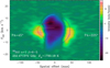 |
Fig. 7 Position-velocity diagram in the direction from PA = 45° to 225° obtained from the continuum-subtracted channel maps of the 30SiO line (v = 1, J = 6–5). The pink, red, and light blue curves at the negative spatial offsets (on the side of PA = 45°) represent the traces expected from shells infalling at velocities of 2 km s−1 at a radius of 75 mas, 7 km s−1 at 50 mas, and 13 km s−1 at 42 mas, respectively. The blue curve on the PA = 225° side shows the trace from an infalling or outflowing (although infalling is more plausible) shell with a velocity of 12 km s−1 at a radius of 45 mas. See Sect. 4.4. |
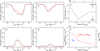 |
Fig. 8 Spherical LTE model for the 30SiO v = 1 J = 6–5 and 29SiO v = 3 J = 6–5 lines. Panels a and b show a comparison between the model (black) and the spectra of the 30SiO v = 1 line (red) observed over the stellar disk and off the limb of the disk (positions 2 and 6 in Fig. 4), respectively. Panels c and d show a comparison for the 29SiO v = 3 line in the same manner. The velocity profile of the model is shown in panel e. Positive and negative velocities correspond to infall and outflow, respectively. Panel f shows the 29SiO number density (assumed to be equal to that of 30SiO) on the left ordinate and the gas temperature on the right ordinate. In panels e and f, the radius is shown in the units of Rcont (below) and R⋆ (above). |
4.6 Si17O v = 0, J = 6–5 at 250.745 GHz
Figure 9 shows the channel maps obtained for the Si17O line (v = 0, J = 6–5) at 250.745 GHz. The maps at velocities more redshifted than Vrel = 9.0 km s−1 are dominated by the 30SiO v = 2 line described in Sect. 4.3. The Si17O maps reveal the same structures as found in the 30SiO v = 1 line – the NNW plume, the SSE tail, and the extended atmosphere elongated in the ENE–WSW direction. Given the upper level energy of mere 42 K, much lower than the other SiO lines discussed above, this Si17O line can be excited across a very broad radial range, extending to cooler regions at larger distances from the star. The images obtained from Vrel = 0 to 3 km s−1 show irregularly shaped emission extending out to a radius of ~120 mas (= 4 Rcont = 5.8 R⋆). Given the largest recoverable scale of 190 mas (i.e., a radius of 95 mas), it is possible that some extended Si17O emission is missing. It is worth noting that the channel maps at Vrel = 1.5–6 km s−1 show that the emission goes inside the stellar limb, in a manner similar to the 30SiO v = 2 line at 250.728 GHz discussed in Sect. 4.3. The emission from the Si17O line covers a larger fraction of the stellar disk than the 30SiO v = 2 line.
The spectra obtained over the stellar disk (Fig. 4, left column, blue lines) show broad absorption, with the deepest absorption centered at Vrel = −4 to −5 km s−1. In addition, the spectra obtained at position 0,1, and 4 show a narrow absorption feature at Vrel ≈ −5 km s−1, which is due to the absorption by the material in the wind that has reached the terminal velocity. Takigawa et al. (2017) and Hoai et al. (2022) also detected narrow features at ~−5 km s−1 originating from the wind at the terminal velocity in the 29SiO v = 0 J = 8–7 line and in the CO v = 0 J = 3–2 line (this latter in emission, which Vlemmings et al. 2021 interpret as maser emission6). The emission covering the stellar disk at Vrel = 1.5–6 km s−1 appears as a bump at 4–5 km s−1 in the spectra except at position 0, although not definitive at position 2.
Surprisingly, the deep redshifted absorption seen in the 30SiO v = 1 line is not observed in Si17O v = 0, although we expect the cool Si17O-bearing gas at outer radii to produce similar, if not stronger, absorption. This suggests that there is anomalous emission over the stellar disk. Assuming that, under thermal excitation, the underlying Si17O absorption is as strong as that of the 30SiO (v = 1), the excess Si17O emission is approximately 20 mJy/beam to fill in the deep absorption and result in the emission bump at Vrel = 4 to 5 km s−1. The emission intensity is comparable to the continuum intensity of ~40 mJy/beam of the stellar disk. However, similar emission over the stellar disk is not observed in the 30SiO v = 1 line, indicating that the Si17O emission is nonthermal – suprathermal or maser. The nonthermal emission is redshifted by 4 to 5 km s−1, as in the case of the 30SiO v = 2 line (Sect. 4.3) and the likely maser emission of the v2 = 2 H2O line at 268 GHz reported in Paper I.
To better visualize the spatial distribution of the suprathermal or maser emission, we created a set of difference maps by subtracting the channel maps of the 30SiO v = 1 line from those of the Si17O v = 0 line. Figure B.1 shows the resulting difference channel maps. Only the maps between Vrel = −4.5 and 7.5 km s−1 are presented, because the data at velocities more blueshifted than Vrel = −4.5 km s−1 and more redshifted than 7.5 km s−1 are affected by the blend of the H2O v2 = 2 line (Sect. 4.8) and the 30SiO v = 2 line (Sect. 4.3), respectively. The figure reveals that the emission is covering the stellar disk and slightly outside the limb at Vrel = 0 to 7.5 km s−1. At the systemic velocity, the excess emission is seen in the NNW, which corresponds to the strong emission in the NNW plume. The images at Vrel = 3.0 to 6.0 km s−1 show bright emission in the western region of the stellar disk.
The large extension of the Si17O emission allows us to probe the dynamics at larger distances than with other SiO lines. The spatially resolved spectra extracted off the limb of the stellar disk at 90 mas (Figs. 4m–4o, blue lines) show that the blue part is noticeably weaker than the red part, which can be interpreted as due to self-absorption in the outflow, as in the case of the HCN line discussed in Sect. 4.12. The same trend is seen in the 30SiO v = 1 line (Figs. 4m–4o, green lines), although the intensity is lower. These results suggest a global outflow at 90 mas (3 Rcont = 4.3 R⋆).
We also find very diffuse emission that is difficult to recognize in the individual channel maps. Figure B.2 shows spectra derived by integrating the intensity in different annular regions. The emission clearly appears in the spectra from the annular regions up to an outer radius of 900 mas (30 Rcont = 43 R⋆), ranging from Vrel = −10 to +10 km s−1. The spectrum obtained from the annular regions from 900 mas to 1200 mas (Fig. B.2d) shows possible emission, but it cannot be considered to be definitive given its low S/N. Moreover, given the largest recoverable scale of 190 mas, weaker and/or smoother emission should be missing, and the detected diffuse emission probably represents only a fraction of the real extended emission. We do not find such diffuse emission in other SiO lines and other molecular lines described below except for the SO and HCN lines.
We note that there is another absorption feature centered at Vrel = −16 to −18 km s−1 in the spectra of the Si17O v = 0 line extracted over the stellar disk (Figs. 4b–4f), which is not seen in any other SiO lines. In the spectrum taken at PA = 225°, this absorption is less pronounced, and it blends with the absorption centered at Vrel = −4 to −5 km s−1, forming a single, very broad absorption trough. Paper I tentatively identified it as the vibrationally excited H2O line (v2 = 2,92,8−83,5). We discuss this issue in more detail in Sect. 4.8.
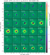 |
Fig. 9 Continuum-subtracted channel maps of W Hya obtained in the Si17O v = 0 J = 6–5 line at 250.744695 GHz, shown in the same manner as Fig. 3. The signals in the images at Vrel ≥ 9 km s−1 are due to the 30SiO v = 2 J = 6–5 line. |
4.7 29SiO v = 2, J = 6–5 at 253.703 GHz
We detect strong masers in the 29SiO v = 2 J = 6–5 line at 253.703469 GHz. The channel maps of the continuum-subtracted images, shown in Fig. 10, reveal three major maser clouds in the east, NNW, and WSW, where the peak intensity reaches ~18 Jy/beam at Vrel = −1.5 to 0 km s−1. As mentioned in Sect. 3, the images at the spectral channels with the strong maser emission are limited by the dynamic range, resulting in RMS noise of 0.8, 2.0, 2.7, and 0.7 mJy/beam at Vrel = −3.0, −1.5, 0, and 1.5 km s−1, respectively, while it is ~0.5 mJy/beam at other spectral channels. The peak intensity of 18 Jy/beam corresponds to a brightness temperature of 106 K. The three major maser clouds are located at a radius of ~50 mas (~2.4 R⋆). Reid & Menten (2007) and Imai et al. (2010) show that the 43 GHz 28SiO maser spots toward W Hya are distributed in a partial ring-like structure at radii of 40–50 mas, which is in qualitative agreement with our ALMA data. The 29SiO masers imaged with ALMA probably consist of a number of individual spots such as those revealed by radio observations at milliarcsecond resolution (e.g., Imai et al. 2010).
Figures B.3g–B.3j show the spatially resolved spectra extracted at four different positions over the maser clouds as marked in Fig. B.3a. The spectra (green lines) are narrow and centered approximately at the systemic velocity. Therefore, the masers are primarily tangentially amplified as in the case for the 43 GHz SiO masers, suggesting that the 29SiO masers detected in our ALMA data likely originate from the same radial range as the 43 GHz masers. However, a closer look at the line profiles extracted from the maser clouds off the limb of the stellar disk reveals the presence of broad components (the blue lines in Figs. B.3g–B.3j).
While the channel maps at Vrel = −10.5 to −1.5 km s−1 show absorption over the stellar disk, emission is detected over the stellar disk between Vrel = −3 to 9.0 km s−1 (i.e., excess emission on top of the continuum). In particular, enhanced emission is seen in the western region of the stellar disk at Vrel = 3.0 to 7.5 km s−1. These western blobs are close to, but do not exactly coincide with, the excess emission in the difference maps of Si17O (Fig. 9) and the channel maps of SO2 line #9 (Sect. 4.9, Fig. 12). The spatially resolved spectra extracted over the stellar disk (Figs. B.3b–B.3f) show that the emission is broad, ranging from Vrel = −3 km s−1 to ~10 km s−1, and it reaches 20–60 mJy/beam at Vrel = 0–4 km s−1. This indicates overall infall of the material in front of the star within ~50 mas, which is consistent with our modeling of the SiO lines (Fig. 8e). Also plotted in Figs. B.3b–B.3f (orange lines) are the spectra of the vibrationally excited H2O line (v2 = 2, 65,2−74,3) at 268 GHz (reported in Paper I), extracted at the same positions as the 29SiO masers. The spectra over the stellar disk show that both lines show strong, broad emission at the redshifted velocities up to 8–12 km s−1, while the emission is weak or it turns to absorption at the blueshifted velocities.
The emission excess over the stellar disk of the H2O and SiO lines cannot be accounted for by the tangential maser amplification. As discussed in Paper I, the density and gas temperature fulfill the conditions for the radiative pumping of the H2O masers, and therefore, the line may easily turn to masers. In the case of the 29SiO maser, which was first discovered in the RSG VY CMa by Cernicharo & Bujarrabal (1992), Herpin & Baudry (2000) show that it can be produced by the line overlaps between infrared ro-vibrational transitions of 29SiO and 28SiO/30SiO. Humphreys et al. (2002) detected occasional 43 GHz SiO maser spots over the stellar disk of the Mira star TX Cam. Their models including pulsation-induced velocity variations in the atmosphere indeed predict occasional appearance of maser spots over the stellar disk by the radial amplification, in addition to the predominantly tangentially amplified masers outside the limb of the stellar disk. Therefore, the emission excess over the stellar disk suggests that the radial amplification is effective to some extent in the 253 GHz 29SiO line. Alternatively, it is also possible that the broad emission over the surface is suprathermal but not masers, while the intense emission off the stellar disk limb is tangentially amplified masers.
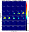 |
Fig. 10 Continuum-subtracted channel maps of W Hya obtained for the 29SiO v = 2 J = 6–5 line at 253.703469 GHz, shown in the same manner as Fig. 3, except that the unit of the color scale is different from other channel maps to show the strong maser emission and weaker emission over the stellar disk. |
4.8 Tentative identification of the vibrationally excited H2O line (v2 = 2,92,8−83,5)
The spectra of the Si17O v = 0 line extracted over the stellar disk show an absorption feature at Vrel = −16 to −18 km s−1 with respect to the Si17O line (Figs. 4b–4f). In Paper I, we tentatively attributed this absorption to the vibrationally excited H2O line (v2 = 2, 92,8−83,5, Eu = 6141 K), at a rest frequency of 250.756834 GHz (Furtenbacher et al. 2020a) or 250.758302 GHz (Furtenbacher et al. 2020b). We describe here details of this tentative identification.
While the frequency of the 268 GHz H2O line is very accurately measured in the laboratory by Pearson et al. (1991) with an error of 0.15 MHz as quoted in the JPL catalog, the transition v2 = 2, 92,8−83,5 has never been measured in the laboratory, and there are noticeable differences among various calculations. Table 3 lists a few selected examples. The latest JPL catalog for vibrationally excited H2O reports a rest frequency of 250.7517934±0.0362551 GHz for this transition (first row in Table 3, Yu et al. 2012). If this frequency is adopted, not only the absorption observed over the stellar disk but also the emission off the disk limb is blueshifted by ~6 km s−1. Given that the emission off the limb is expected to be roughly centered around the systemic velocity in the case of globally spherical motion, the systematic blueshift of the emission off the limb is difficult to interpret.
Recently, Furtenbacher et al. (2020a,b) produced the W2020 database of validated experimental transitions and empirical energy levels of H2O. If we adopt the empirical energies as shown in Table 3, the line frequencies of the 251 GHz transition are 250.756834 ± 0.001242 GHz and 250.758302 ± 0.000925 GHz, respectively. With these values, both the observed absorption and emission appear approximately at the systemic velocity as seen in Fig. 2 of Paper I. As Table 3 shows, the differences in the frequency originate from the energy of the upper state (v2 = 2, JKa Kc = 92,8), which is less constrained by experimental transitions than the lower state. Moreover, the upper level energy is considered slightly less reliable in the updated W2020 database (Furtenbacher et al. 2020b) than its original version. Our tentative identification of the H2O v2 = 2,92,8−83,5 line suggests that the upper state energies from Furtenbacher et al. (2020a,b) agree with the observation.
We also considered the possibility that the absorption blueshifted by 16 km s−1 with respect to the Si17O line rest frequency originates from Si17O itself in an outflow, instead of the H2O line. However, we deem it to be unlikely, because the other SiO lines do not show such salient absorption blueshifted by 16–18 km s−1. Another possibility is that it can be explained by a clumpy cloud outflowing at 16–18 km s−1 just covering the stellar disk in front of the star in cool, far regions where the other SiO lines with much higher upper level energies cannot be excited. However, such a scenario seems to be too fortuitous.
We also checked whether this absorption is due to molecules other than H2O and Si17O. On the Splatalogue line list, there is an 17OH line (vrest = 250.757411 GHz), which corresponds to a velocity shift of −15.2 km s−1 with respect to the Si17O line. However, it is unlikely that the absorption at issue is attributed to 17OH for the following reason. There is another 17OH line (vrest = 250.742102 GHz), which corresponds to a velocity shift of 3.1 km s−1 with respect to the Si17O line. The upper level energy of this line is the same as the one at −15.2 km s−1 but the Einstein coefficient Aul is 48 times larger. Therefore, we expect to see absorption at 3.1 km s−1 stronger than that at −15.2 km s−1. However, the observed spectra show no absorption at 3.1 km s−1, which makes it very unlikely that the absorption centered at Vrel = −16 km s−1 is due to 17OH. Therefore, the vibrationally excited H2O line (v2 = 2, 92,8−83,5) is the most likely candidate for the absorption feature.
Upper and lower level energies and the rest frequency of the H2O v2 = 292,8−83,5 line from different databases.
4.9 SO2 lines
Figures 11 and 12 show the channel maps of two representative SO2 lines in the ground vibrational state v = 0. The remaining SO2 lines identified in the current work are presented in Figs. C.1–C.19. For very weak SO2 lines, it is difficult to recognize signals in the channel maps. However, the signatures of the SO2 lines could be detected in the integrated intensity maps, which are shown in Fig. C.20. The extended emission of the SO2 lines seen in the channel maps is similar to that observed in the lines of 30SiO v = 1 and Si17O v = 0. The NNW plume extends to a radius of ~100 mas (~3.3 Rcont = 4.8 R⋆), while the SSE tail can be seen up to a radius of ~120 mas (~4 Rcont = 5.8 R⋆). The extended atmosphere elongated in the ENE-WSW direction has approximately the same angular size as seen in the 30SiO v = 1 and Si17O v = 0 lines.
It is worth noting that the channel maps of the SO2 line #9 (Fig. 12) reveal clear emission over the stellar disk at Vrel = −1.5 to 7.5 km s−1. In particular, there is a salient emission spot in the western half of the stellar disk, which appears to be the strongest at 3 km s−1 and reaches ~8.5 mJy/beam above the continuum or 2588 K in brightness temperature. Only in the NE region of the stellar disk does the line appear in absorption as expected for thermal excitation. The western emission is also close to the excess emission seen in the lines of Si17O (Sect. 4.6, Fig. 9) and 29SiO (Sect. 4.7, Fig. 10). The emission over the stellar disk on top of the continuum is seen in the channel maps of other detected SO2 lines, but not always located in the same regions of the disk.
We also checked whether the SO2 lines in the ground and vibrationally excited states detected with low S/N show emission or absorption over the stellar disk by measuring the flux within a radius of 30 mas from the continuum-subtracted data. We also measured the flux in an annular region with an inner and outer radius of 30 and 90 mas, respectively, to confirm the detection of the emission. Figure C.21 shows that the emission from the annular region is indeed detected in all cases. Only three lines (panels a, c, and k) show absorption over the stellar disk (the blueshifted absorption in the v= 0 636,58−627,55 line in panel g is due to the blend of the SO v = 0 NJ = 43−34 line). Six lines show emission (panels d, f, h, j, l, and o), and there are three lines that show both emission and absorption on the stellar disk (panels m, n, and p). The remaining lines (panels b, e, and i) show neither clear absorption nor emission. As in the case of the 30SiO v = 2 and Si17O v = 0 lines, the emission on top of the continuum over the stellar disk is considered to be of nonthermal origin, suprathermal or maser emission. Our results reveal that the majority of the detected SO2 lines exhibit nonthermal emission over the stellar disk.
Danilovich et al. (2016, 2020) report the detection of a number of SO2 lines toward a small sample of AGB stars. More recently, Wallström et al. (2024) present the detection of many vibrationally excited SO2 lines in a larger sample of AGB stars and RSGs. While the stellar disks were not spatially resolved by the observations of Danilovich et al. (2016), their modeling of the W Hya data shows SO2 forms close to the star, down to 2 × 1014 cm (= 6.7 R⋆) or even closer. The ALMA observations of Danilovich et al. (2020) of the low mass-loss rate (a few × 10−7 M⊙ yr−1) AGB star R Dor, whose mass-loss rate is low and similar to that of W Hya, show that SO2 forms close to the star, with its intensity peaking within the continuum emission. Our high-angular-resolution ALMA images of W Hya confirm that SO2 indeed forms very close to the star, down to ~2 R⋆.
Also, Danilovich et al. (2016) present likely maser emission of the vibrationally excited SO2 (v2 = 1254,22−261,25) line at 279.497 GHz in R Dor. Vlemmings et al. (2017) report the detection of a vibrationally excited SO2 line at 342.436 GHz (v2 = 1, 233,21−232,22, Eu = 1021 K) toward W Hya and tentatively identify another SO2 line at 345.017 GHz (v2 = 2,273,25−280,28, Eu = 1832 K). Interestingly, the line at 345.017 GHz detected by Vlemmings et al. (2017) appears in emission over the stellar disk with a FWHM of 7.3 ± 0.6 km s−1, just as many of the SO2 lines detected in our ALMA observations.
We carried out a population diagram analysis to estimate the excitation temperature and column density of SO2, assuming LTE and that the lines are optically thin. While we detect 27 SO2 lines, many of them show nonthermal emission over the stellar disk. Therefore, we selected only the SO2 lines that show no emission on top of the continuum over the stellar disk at any frequencies across the lines, which are the lines #8, #12, #13, #19, #22, and #26 (we excluded the line #33 shown in panel k in Fig. C.21 due to possible blend of the adjacent strong SO line #41). We measured the line flux of the emission off the stellar disk by integrating across the line profile in two annular regions between a radius of 30 and 60 mas (i.e., between 1 and 2 Rcont or ~1.5 and 3.0 R⋆) and between 60 and 100 mas (between 2 and 3.3 Rcont = ~3 and 5 R⋆, approximately up to the largest recoverable scale) to derive the properties in the innermost and intermediate regions, respectively. The error in the absolute flux calibration was assumed to be 10% (ALMA Technical Handbook, Cortes et al. 2025).
Figure 13 shows that the measurements are reasonably fit with an excitation temperature (Tex) of 750 K and a column density (Nso2) of 4.6 × 1018 cm−2 in the innermost region, while the data in the intermediate region result in Tex = 720 K and NSO2 = 1.9 × 1018 cm−2. The uncertainties in the Tex and Nso2 are ±100 K and 46% in the inner region and ±90 K and 42% in the intermediate region, respectively. The fit in either region suggests that LTE is fairly valid for the selected lines. We also calculated the optical depth of the lines using Eq. (27) of Goldsmith & Langer (1999) and confirmed that the optical depth is ≲0.7 for the selected lines, lending support to the population diagram analysis.
To obtain the fractional abundance of SO2 with respect to H2, we estimated the H2 column density as follows. The pulsation+dust-driven wind models of Bladh et al. (2019) show mass densities of 10−12−10−11 g cm−3 at ~1 Rcont ≈ 1.5 R⋆, which translate into H2 number densities of 3 × 10¹¹−3 × 1012 cm−3. Assuming a density profile ∝ r−2, we computed the H2 column density along each line of sight and then the value averaged over two annular areas. The averaged H2 column density is 2.8 × 1025−2.8× 1026 cm−2 and 1.6× 1025−1.6× 1026 cm−2 in the innermost and intermediate regions, respectively. Because the density profile in the wind acceleration region can be steeper than α r−2, the H2 column density can be lower. This sets lower limits of ~2 × 10⁻⁸ (innermost region) and ~1 × 10⁻⁸ (intermediate region) on the fractional SO2 abundance with respect to H2.
The chemical equilibrium model of Agúndez et al. (2020) predicts a fractional SO2 abundance lower than a few ×10−10 at 2–5 R⋆ in an O-rich case, which is 50–100 times lower than the lower limits derived above. We note that if we adopt the temperature and pressure profiles of Agúndez et al. (2020)7, the H2 column density averaged over the innermost annular area is ~8 × 1025 cm−2, which does not improve the disagreement.
The nonequilibrium chemistry model of Gobrecht et al. (2016) predicts the formation of SO in weak shocks at low post-shock temperatures at ≳3 R⋆ through S + OH → SO + H and SH + O → SO + H, and the subsequent formation of SO2 through SO + OH → SO2 + H. The predicted SO2 fractional abundance remains a few ×10−9 at 3 R⋆ during most of the phase, which is lower than our observationally estimated values, but it reaches ~4 × 10⁻⁸ at ~4 R⋆ just before a shock passage. Because their model is not specifically constructed for W Hya, this may be regarded as fair agreement with our observationally estimated value of ≳1 × 10⁻⁸ in the intermediate region. Still, given the phase dependence of the abundance, multi-epoch observations and full non-LTE radiative transfer modeling are necessary to test the nonequilibrium chemistry models.
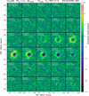 |
Fig. 11 Continuum-subtracted channel maps of W Hya obtained in the SO2 line (v = 0 JKa,Kc = 3610,26−379,29) at 250.816786 GHz, shown in the same manner as Fig. 3. |
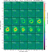 |
Fig. 12 Continuum-subtracted channel maps of W Hya obtained in the SO2 line (v = 0 JKa,Kc = 324,28−315,27) at 252.563893 GHz, shown in the same manner as Fig. 3. |
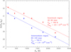 |
Fig. 13 Population diagram for the SO2 lines without signatures of nonthermal emission in the innermost and intermediate regions defined as annular areas between 30 and 60 mas (~1 and 2 Rcont) and between 60 and 100 mas (~2 and 3.3 Rcont), respectively. The red and blue dots represent the measurements in the innermost and intermediate regions, respectively. The solid red and blue lines represent the fits in the respective regions. The excitation temperatures (Tex) and column densities (NSO2) derived in two regions are also shown. |
4.10 34SO2 lines
We detect four 34SO2 lines in the ground vibrational state, and the channel maps are shown in Figs. C.22–C.24 and Fig. C.7 (this last line is blended with an SO2 line). The morphology of the emission is similar to the SO2 lines. The emission appears to be clumpy, partially due to lower S/N than in other stronger SO2 lines. The 324,28−323,29 line appears in absorption over the stellar disk. In other two lines, the S/N is not high enough to recognize the morphology of the extended emission, although the channel maps at −1.5 to +1.5 km s−1 of the 153,13−152,14 line (Fig. C.23) seem to hint the similar morphology as other SO2 lines. In the case of the 95,5−104,6 line (Fig. C.24), the emission appears at −6 to 0 km s−1, indicating a blueshift of the 34SO2 line. We note that there is a TiO2 line (276,22−275,23, Eu = 317 K) at 252.617051 GHz, which corresponds to a velocity shift of −2 km s−1 with respect to the 34SO2 line. However, as we discuss in Sect. 4.14, TiO2 emission is generally very weak, and the contribution of this TiO2 line is likely negligible compared to that of the 34SO2 line.
4.11 SO lines
We detect two SO lines, NJ = 65−54 at 251.825770 GHz and NJ = 43−34 at 267.197746 GHz. We describe here only the first SO line (line #41), because the other line is of low S/N, and it is also blended with neighboring SO2 and HCN lines (the channel maps of this weak SO line are shown in Fig. C.25). Figure 14 shows the channel maps obtained for the NJ = 65−54 SO line (note that the field of view of 550×550 mas is larger than that of the SiO, H2O, and SO2 lines presented above). We can recognize the NNW plume and the SSE tail, and the images taken near the systemic velocity show the extended atmosphere elongated in the ENE-WSW direction.
However, the SO emission is more extended than that of the SO2 lines. The NNW plume also extends farther to form an arm that winds and extends to the NE between Vrel = −7.5 to −1.5 km s−1. This can be an outflow in front of the plane of the sky or an infall behind the plane of the sky. The arm extends relatively far from the star to a radius of ~150 mas (~7.2 R⋆). We deem an outflow to be more plausible, because the Si17O v = 0 emission indicates a global outflow already at 90 mas (~4.3 R⋆) as discussed in Sect. 4.6. The SO emission extends beyond the largest recoverable radius of ~95 mas (corresponding to a half of the largest recoverable scale of 190 mas). Nevertheless, emission at a radius larger than 95 mas can still be detected as far as it is sufficiently compact in a form of plumes or filaments. Therefore, the northern arm is likely real, while smooth extended emission may not be fully recovered.
Figure C.26 (left column) shows the spatially resolved spectra extracted at the same five positions over the stellar disk as for the SiO lines (as labeled in panel a). The spectra show narrow absorption features at Vrel = −5 km s−1, as seen in Si17O, which originates from the wind that has reached the terminal velocity. The broad, overall absorption shows the deepest points at Vrel = 2–3 km s−1. The absorption at positions 0,1, and 2 is particularly broad, extending from Vrel = −20 to 15 km s−1. On the other hand, the spectra extracted outside the stellar disk (Figs. C.26g–C.26j) show emission only to about ±10 km s−1, not up to ±20 km s−1. This implies that the high-velocity absorption wings originate from the region close to the star as in the case of the high excitation 29SiO v = 3 line that originates from the region within ~2 R⋆. As mentioned in Sect. 4.2, the escape velocity at 1.9 R⋆ is 21 km s−1. The most blueshifted wing of the SO line extending to Vrel ≈ −20 km s−1 suggests the presence of material almost at the escape velocity at ~2 R⋆. The detection of SO close to the star is consistent with the analysis of W Hya by Danilovich et al. (2016), who show that SO forms 2 × 1014 cm (= 6.7 R⋆) or even closer.
Danilovich et al. (2020) also report that the SO2 and SO emission trace the same structures in the low mass-loss rate AGB star R Dor. Our ALMA observations show that this seems to be the case for the NNW plume, SSE tail, and the elongated atmosphere of W Hya, which can be seen in both SO2 and SO. We compare the channel map at the systemic velocity of the SO line and SO2 line #12, because this latter line has an upper level energy of 106 K, which is the closest to that of the SO line (51 K). Figure C.27 shows the azimuthally averaged 1D intensity profiles of the SO and SO2 lines. The SO emission is more extended primarily due to its lower upper level energy. Nevertheless, there is a hint that the intensity peak of the SO2 line is slightly farther away than that of the SO line, in spite of the higher upper level energy of the SO2 line, suggesting that the SO2 abundance may peak slightly outside the SO abundance. We note that the full range of the excitation energy of SO2 is not probed in the present work unlike the study of Danilovich et al. (2020), and therefore, we do not have observational constraints farther out. High-angular-resolution ALMA imaging dedicated to SO2 and SO lines (e.g., in Band 7), combined with a compact configuration or a single-dish telescope, are necessary to investigate the detailed SO2 and SO distribution at beyond ~5 R⋆.
Because we detect only two SO lines, and the NJ = 43−34 line (#42) is of low S/N and blended with the SO2 and HCN lines, we cannot apply the population diagram analysis. We estimated the SO column density in the same annular regions as used for the SO2 lines (Sect. 4.9) from the NJ = 65−54 line (#41) alone by assuming the excitation temperatures derived from the SO2 lines. The resulting area-averaged SO column densities are 7.0 × 1017 cm−2 in the innermost region between 30 and 60 mas (between 1 and 2 Rcont ≈ 1.5–3 R⋆) and 3.0 × 1017 cm−2 in the intermediate region between 60 and 100 mas (between 2 and 3.3 Rcont ≈ 3–5 R⋆). Adopting higher or lower excitation temperatures of 1000 K and 500 K leads to an uncertainty in the SO column density by a factor of ~2. These column densities translate into fractional SO abundances of ≳ 3 × 10⁻⁹ and ≳2 × 10⁻⁹ in the innermost and intermediate regions, respectively, if the H2 column densities estimated in Sect. 4.9 are adopted. It should also be kept in mind that we may be missing the extended, smooth emission as mentioned above, which can lead to even higher SO abundances.
The derived lower limits on the SO abundance are in broad agreement with the chemical equilibrium model of Agúndez et al. (2020), which predicts abundances of 10−8−10−7 within ~5 R⋆. The nonequilibrium model predicts the SO abundance of a few ×10−8−10−7 within ~5 R⋆ (Gobrecht et al. 2016), which is also consistent with the observational lower limits. As mentioned in Sect. 4.9, SO forms in weak shocks, followed by the subsequent formation of SO2 at slightly larger radii in the nonequilibrium chemistry model (see Fig. 4 of Gobrecht et al. 2016). This is qualitatively consistent with the 1D intensity peak positions of the SO and SO2 lines shown in Fig. C.27. However, Gobrecht et al. (2016) mention that SO2 does not form efficiently by the reactions of SO and OH in their model, which is why the predicted SO2 abundance remains lower than the observed values in the literature (see their Table 5). Still, the observed overlap of the SO and SO2 emission suggests some chemical reactions that connect SO2 and SO.
Vlemmings et al. (2011) detected an SO line 55−44 in W Hya at an angular resolution of ![Mathematical equation: $\[{\sim}1^{\prime\prime}_\cdot5 {\times} 1^{\prime\prime}_\cdot0\]$](/articles/aa/full_html/2025/12/aa54900-25/aa54900-25-eq15.png) and found a slight offset of
and found a slight offset of ![Mathematical equation: $\[0^{\prime\prime}_\cdot29\]$](/articles/aa/full_html/2025/12/aa54900-25/aa54900-25-eq16.png) between the integrated red- and blueshifted velocities (their Fig. 7). This led them to consider the possible presence of a bipolar outflow with its axis approximately in the N-S direction or a rotating disk aligned in the N-S direction, although they did not exclude that it might be due to complex kinematical structures. Our channel maps obtained at a higher angular resolution do not show signatures of a bipolar outflow or a rotating disk and indicate that the emission within the largest recoverable scale (i.e., within a radius of ~95 mas = ~4.6 R⋆) is primarily influenced by the complex kinematical structures. However, as presented below, the SO emission is much more extended than the largest recoverable scale, and therefore, we cannot examine the kinematical structures on larger spatial scales.
between the integrated red- and blueshifted velocities (their Fig. 7). This led them to consider the possible presence of a bipolar outflow with its axis approximately in the N-S direction or a rotating disk aligned in the N-S direction, although they did not exclude that it might be due to complex kinematical structures. Our channel maps obtained at a higher angular resolution do not show signatures of a bipolar outflow or a rotating disk and indicate that the emission within the largest recoverable scale (i.e., within a radius of ~95 mas = ~4.6 R⋆) is primarily influenced by the complex kinematical structures. However, as presented below, the SO emission is much more extended than the largest recoverable scale, and therefore, we cannot examine the kinematical structures on larger spatial scales.
We also detect diffuse, patchy SO emission extending out to a radius of ~1″ (~33 Rcont = 48 R⋆), as shown in Fig. C.28. Because it is more extended than the largest recoverable scale of 190 mas of our ALMA observations, the detected structures represent high intensity regions embedded in more diffuse emission with lower intensities. The complex structures seen within 250 mas may give rise to these arc-like structures as they disperse at large distances from the star. Arc-like structures are detected in various AGB stars, and they are often caused by binary companions (e.g., Maercker et al. 2012; Decin et al. 2020; Siebert et al. 2022). However, there is no signature of a binary companion for W Hya reported in the literature. On the other hand, clumpy structures are observed on the surface of some AGB stars (e.g., Vlemmings et al. 2019, 2024; Velilla-Prieto et al. (2023), probably associated with convective cells of sizes comparable to the stellar radius. The 3D dynamical models of Freytag & Höfner (2023) show that the convective cells expand as the material is accelerated and form a collection of partial arcs at radii greater than 3–4 R⋆. Therefore, the arc-like structures of the SO line detected up to ~1″ toward W Hya can be a consequence of this process.
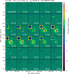 |
Fig. 14 Continuum-subtracted channel maps of W Hya obtained in the SO line (v = 0, NJ = 65−54) at 251.825770 GHz, shown in the same manner as Fig. 3 but for a field of view of 550×550 mas. In addition, the insets show the enlarged view (80×80 mas) of the signal over the stellar disk. |
4.12 HCN lines
We detect three HCN lines in our ALMA observations: v = 0, J = 3–2 at 265.886434 GHz, v2 = 11e, J = 3–2 at 265.852709 GHz, and v2 = 11f, J = 3–2 at 267.199283 GHz. The data of the ground-state transition show detailed morphological and kinematical structures as described below. On the other hand, S/N of ≲ 5 of the individual channel maps of the two vibrationally excited lines is not sufficient to discuss such structures, as shown in Figs. C.25 and D.1 for completeness. To better visualize the signals of the v2 = 11e line, we created an integrated intensity map from the channel maps reconstructed with the natural weighting (Fig. 16). The v2 = 11f line is blended with SO, and therefore, we do not discuss it in the present work.
The ground-state HCN line consists of six hyperfine structure transitions. The three strongest components, F = 4–3, 3–2, and 2–1, carry most of the intensity of the rotational transition (Ahrens et al. 2002), and they are closely spaced within a velocity difference of 0.35 km s−1, which is smaller than the velocity resolution of our data. Therefore, we treat HCN v = 0 as a single line in the present work and adopt the rest frequency of 265.886434 GHz from CDMS, which also corresponds to the weighted mean of the hyperfine components.
Figure 15 shows the channel maps obtained for the ground-state HCN line8. Its emission is by far more extended than other SiO, SO2, and SO lines. As discussed below, the entire HCN emission extends beyond the field of view of 550×550 mas of the figure, out to a radius of ~1″. The extended emission is more prominent at the redshifted velocities than at the blueshifted velocities. This is also seen in the spectra extracted at different positions, shown in Figs. D.2g–D.2j, which reveal that the emission is stronger in the red wing than in the blue wing except for positions 11 and 25 at PA = 165°, where the line profiles are approximately symmetric.
The observations of the same HCN line toward W Hya with a lower spatial resolution of ![Mathematical equation: $\[0^{\prime\prime}_\cdot55 {\times} 0^{\prime\prime}_\cdot40\]$](/articles/aa/full_html/2025/12/aa54900-25/aa54900-25-eq17.png) using the Submillimeter Array (SMA) also show that the red wing of the emission is more prominent than the blue wing (Müller et al. 2008). As these authors explain, the observed asymmetry in the line profile is due to the self-absorption caused by colder HCN gas in the outer region. In an expanding envelope, the blueshifted emission originates from the hemisphere on the near side, while the redshifted emission originates from the gas behind the plane of sky. Because the HCN emission is optically thick as shown below, we see the radiation from the layer with an optical depth of 1 along the line of sight. Assuming approximately spherical expansion, at a given relative velocity, the blueshifted emission originates from cooler HCN gas (and thus lower brightness temperature) at larger radii on the near-side hemisphere due to self-absorption, while the redshifted emission originates from warmer gas (i.e., higher brightness temperature) at smaller radii on the far-side hemisphere.
using the Submillimeter Array (SMA) also show that the red wing of the emission is more prominent than the blue wing (Müller et al. 2008). As these authors explain, the observed asymmetry in the line profile is due to the self-absorption caused by colder HCN gas in the outer region. In an expanding envelope, the blueshifted emission originates from the hemisphere on the near side, while the redshifted emission originates from the gas behind the plane of sky. Because the HCN emission is optically thick as shown below, we see the radiation from the layer with an optical depth of 1 along the line of sight. Assuming approximately spherical expansion, at a given relative velocity, the blueshifted emission originates from cooler HCN gas (and thus lower brightness temperature) at larger radii on the near-side hemisphere due to self-absorption, while the redshifted emission originates from warmer gas (i.e., higher brightness temperature) at smaller radii on the far-side hemisphere.
The HCN spectra obtained at different angular distances at a given position angle are nearly identical (Figs. D.2g–D.2j), which suggests that the line is optically thick. The spectrum at position 7 is somewhat different, presumably because it originates from a bright clump. The spectra extracted over the stellar disk are shown in Figs. D.2b–D.2f. Because the line is optically thick, the brightness temperature (shown in the right ordinate) allows us to estimate the gas temperature of the HCN line formation. Given that the three strongest hyperfine structure components appear to be a single component as mentioned above, the narrow, deep absorption seen at Vrel = −5 km s−1 is attributed to the wind that has reached its terminal velocity9. The brightness temperature at the deepest absorption at −5 km s−1 ranges from ~150 to ~200 K.
We estimated the radius that corresponds to these brightness temperatures, using the power-law temperature distributions derived for the circumstellar envelope of W Hya. (Müller et al. 2008) derived Tgas(r) (K) = 650 (1014/r(cm)) based on the radial intensity profile of the HCN (v = 0, J = 3–2) line alone. On the other hand, Khouri et al. (2014a) obtained Tgas(r) (K) = 2500 (2.7 × 10¹³/r(cm))0.65, which was constrained by multiple single-dish CO spectra from J = 1–0 (Eu = 5.5 K) to J = 24–23 (1656 K). With the model of (Müller et al. 2008), the temperatures of 150–200 K correspond to radii of (3.2–4.3) × 1014 cm (= 11–14 R⋆). The escape velocity at these distances is 8–9 km s−1, which is higher than the terminal velocity of 5 km s−1 for a 1 M⊙ star. This contradicts that the deepest absorption dip originates from the wind that has reached the terminal velocity. On the other hand, if we adopt the temperature profile of Khouri et al. (2014a), the observed temperatures of 150–200 K are reached at (1.3–2.0) × 1015 cm (43–67 R⋆) with a local escape velocity of 3.7–4.5 km s−1, lower than the wind terminal velocity (the local escape velocity drops to 5 km s−1 already at ~1.06 × 1015 cm = 35 R⋆, corresponding to ![Mathematical equation: $\[0^{\prime\prime}_\cdot72\]$](/articles/aa/full_html/2025/12/aa54900-25/aa54900-25-eq18.png) ). This lends support to the temperature profile from Khouri et al. (2014a). The line profiles show another two absorption dips at Vrel = −2 km s−1 and 2–3 km s−1 (particularly at positions 0, 3, and 4). Both absorption dips indicate possible inhomogeneities along the line of sight at radii where the gas is still gravitationally bound.
). This lends support to the temperature profile from Khouri et al. (2014a). The line profiles show another two absorption dips at Vrel = −2 km s−1 and 2–3 km s−1 (particularly at positions 0, 3, and 4). Both absorption dips indicate possible inhomogeneities along the line of sight at radii where the gas is still gravitationally bound.
A carbon-bearing molecule such as HCN is not expected in the oxygen-rich atmosphere of W Hya in chemical equilibrium. Gobrecht et al. (2016) present the modeling of the formation of HCN in shocks in the dynamical atmosphere. The aforementioned SMA observations by (Müller et al. 2008) show that the HCN emission originates from the region within ~10 R⋆, suggesting that HCN forms in shocks in the inner region of the circumstellar envelope. The optically thick HCN v = 0 line is estimated to originate far away from the star at 43–67 R⋆, as discussed above, and therefore, it does not set a stricter constraint on the HCN formation region. On the other hand, the vibrationally excited (v2 = 11e) HCN line is much weaker and not optically thick. The integrated intensity map of this line (Fig. 16) reveals the presence of HCN close to the star, down to ~30 mas (~1.4 R⋆). The models of Gobrecht et al. (2016) predict the formation of HCN at 1–2 R⋆. The detection of HCN close to the star lends strong support to the idea that HCN forms in shock-induced chemistry in the dynamical atmosphere.
Gobrecht et al. (2016) also show that the HCN abundance drastically decreases in the region where H2 is depleted due to grain nucleation. The contours in Fig. 16 show the polarized intensity map obtained at 820 nm contemporaneously with our ALMA data using VLT/SPHERE-ZIMPOL, as reported in Paper I. The polarized intensity map shows the formation of clumpy dust clouds in the east, SW, and NNW. While the emission of the HCN v2 = 11e line is present in the dust cloud formation regions, the HCN emission does not exactly coincide with the clumpy dust clouds and extends farther out to ~100 mas without showing a signature of depletion. This suggests that the dust formation does not completely deplete H2 as predicted by the model. However, it should be kept in mind that the models of Gobrecht et al. (2016) correspond to IK Tau, whose mass-loss rate is much higher than that of W Hya. Also, the HCN emission can depend on the variability phase. Imaging of HCN lines with higher J at different epochs at higher angular resolutions will be important to address this point.
An alternative model for the presence of HCN in oxygen-rich stars is that HCN forms as a product of photochemical reactions in the circumstellar envelope due to the penetration of interstellar UV photons (Charnley et al. 1995). In this model, HCN is not expected to form in high abundance at the innermost radii, and the emission would be seen as a hollow shell. Van de Sande et al. (2018) investigated the effects of clumping and porosity on the circumstellar chemistry due to deeper penetration of the interstellar UV radiation and enhanced clump density. Their models show that the HCN abundance is generally more enhanced in the inner wind for low mass-loss rates. The predicted HCN abundances increase significantly beyond a few ×1014 cm (~10 R⋆) as seen in their Figs. 4–5. Agúndez et al. (2010) obtained similar results (their Fig. 3). These results are not consistent with the presence of HCN close to the star, down to ~1.4 R⋆, as indicated by the integrated intensity map of the HCN v2 = 11e line.
The modeling with the UV radiation from the AGB star (Van de Sande et al. 2019) also shows that HCN (and also SO in some cases) is destroyed in the innermost regions (their Figs. 4F and 4D), which does not agree with the observation of the HCN v2 = 11e line. The models with the UV radiation from a companion by Van de Sande et al. (2022) show the depletion of SO in the innermost region (their Fig. 3), which is not seen in our ALMA data of the SO line (Fig. 14). In addition, we are not aware of evidence of a companion of W Hya in the literature and in our ALMA data. Therefore, the presence of HCN in the inner wind of W Hya is better explained by the shock-induced chemistry model rather than the photochemistry model. However, photo-chemistry may play an important role for understanding the very extended distribution of the HCN v = 0 line as described below.
Figure D.3 shows the HCN emission in a larger field of view of 2.4″ × 2.4″. On a large scale, the emission morphology appears to be irregular with an apparent elongation in the E-W direction. Across most of the channels with the extended emission, we can recognize clumpy, asymmetric emission within ![Mathematical equation: $\[{\sim}0^{\prime\prime}_\cdot5\]$](/articles/aa/full_html/2025/12/aa54900-25/aa54900-25-eq19.png) and complex filamentary, spider-like structures up to a radius of ~1″ (corresponding to ~33 Rcont = 48 R⋆). However, given the largest recoverable scale of ~190 mas, a significant amount of flux density from diffuse, smooth emission on large angular scales is considered to be missing. In fact, in the aforementioned SMA images obtained by Müller et al. (2008), which recovered >70% of the total intensity within 28″, the HCN emission appears to be smooth and roughly spherically symmetric out to a radius of
and complex filamentary, spider-like structures up to a radius of ~1″ (corresponding to ~33 Rcont = 48 R⋆). However, given the largest recoverable scale of ~190 mas, a significant amount of flux density from diffuse, smooth emission on large angular scales is considered to be missing. In fact, in the aforementioned SMA images obtained by Müller et al. (2008), which recovered >70% of the total intensity within 28″, the HCN emission appears to be smooth and roughly spherically symmetric out to a radius of ![Mathematical equation: $\[1^{\prime \prime}_\cdot 0{-}1^{\prime \prime}_\cdot 5\]$](/articles/aa/full_html/2025/12/aa54900-25/aa54900-25-eq20.png) . Therefore, the filamentary features at the large radii simply represent localized regions with relatively high intensities. For this reason, we are unable to conclude from our images alone if there is indeed a global deviation from spherical symmetry of the HCN emission.
. Therefore, the filamentary features at the large radii simply represent localized regions with relatively high intensities. For this reason, we are unable to conclude from our images alone if there is indeed a global deviation from spherical symmetry of the HCN emission.
Müller et al. (2008) detected a velocity gradient over ![Mathematical equation: $\[0^{\prime\prime}_\cdot5\]$](/articles/aa/full_html/2025/12/aa54900-25/aa54900-25-eq21.png) in the NW-SE direction and suggested that it might be due to a bipolar outflow or a rotating envelope. Our ALMA images do not show such a velocity gradient, and the emission within the largest recoverable scale (i.e., within a radius of ~95 mas) is dominated by the inhomogeneous structures. However, the missing diffuse, smooth emission in our ALMA data does not allow us to study the kinematical structure on larger scales, as in the case of the SO line discussed in Sect. 4.11.
in the NW-SE direction and suggested that it might be due to a bipolar outflow or a rotating envelope. Our ALMA images do not show such a velocity gradient, and the emission within the largest recoverable scale (i.e., within a radius of ~95 mas) is dominated by the inhomogeneous structures. However, the missing diffuse, smooth emission in our ALMA data does not allow us to study the kinematical structure on larger scales, as in the case of the SO line discussed in Sect. 4.11.
Hoai et al. (2022) report enhanced emission in the NNW in W Hya extending to an angular distance of ~150 mas (~7.2 R⋆) at blueshifted velocities, which led the authors to interpret it as an outflowing blob in front of the star. With the distance of 98 pc and a maximum projected velocity of 5 km s−1, which corresponds to the wind terminal velocity, the blob could have traveled an angular distance of 27 mas in 2.5 years between the observations reported in Hoai et al. (2022) and ours. Therefore, the blob should be located at between 150 and 177 mas from the stellar center at the time of our ALMA observations, depending on the projection effect.
The intensity of most of the lines identified in our ALMA data is not sufficient at the angular distance of 150 mas to detect the possible presence of this blob. Only the 265 GHz HCN and 251 GHz SO (Sect. 4.11) lines show detectable emission – albeit still rather weak – at 150–200 mas due to their intrinsically very extended nature. The channel maps of the SO line show very faint emission at the tip of the northern arm at an angular distance of 180 mas at −7.5 km s−1 (Fig. 14), and the HCN channel maps show a blob in the north from Vrel = −9 to −7.5 km s−1 at angular distances of 150–200 mas (Fig. 15). These features may correspond to the blueshifted blob reported by Hoai et al. (2022).
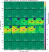 |
Fig. 15 Channel maps of W Hya obtained in the HCN (v = 0, J = 3–2) line at 265.886434 GHz, shown in the same manner as Fig. 3 but in a larger field of view of 550×550 mas. The insets show the enlarged view (80×80 mas) of the signal over the stellar disk. |
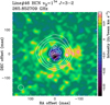 |
Fig. 16 Color map: intensity map of the HCN (v2 = 11e, J = 3–2) line at 265.852709 GHz integrated from Vrel = −10.5 to 10.5 km s−1. Contours: polarized intensity obtained at 820 nm contemporaneously with our ALMA observations (Paper I). The contours are drawn on a logarithmic scale at 10%, 17%, 30%, 52%, and 90% of the peak value. The black circle represents the millimeter continuum stellar disk. The beam size of the HCN intensity map is shown in the lower left corner. |
4.13 AIO and AIOH
We detect the AlO N = 7–6 line near 267.9 GHz (Eu = 51–52 K). Its channel maps, shown in Fig. E.1, reveal that the signature of AlO is present across a wide velocity range from Vrel = −30 to +30 km s−1 due to the presence of multiple hyperfine components of similar strengths between 267.912 and 267.961 GHz. We also detect seven individual hyperfine components that belong to the same transition outside the velocity range shown in the figure. Although their channel maps appear to be too noisy, the intensity maps integrated from Vrel = −5 to 5 km s−1 show the signals of AlO more clearly. We present the images of these weak hyperfine components in Fig. E.2 for completeness.
The AlO emission extends to a radius of 50–80 mas (1.7–2.7 Rcont = 2.4–3.9 R⋆). It is worth noting that the channel maps at all velocities between Vrel = −30 and 30 km s−1 show emission – albeit weak – over the stellar disk. No other line is found at the observed velocity shifts in the Splatalogue, CDMS, JPL, and HITRAN catalogs. Therefore, we interpret the emission over the stellar disk as of the nonthermal origin – suprathermal or weak maser action – as in the case of the SiO and SO2 lines described above.
The spatial extension of the AlO emission in our ALMA data is similar to that of the AlO N = 8–9 line (Eu ≈ 80 K) at 344.4 GHz observed in 2015 (Takigawa et al. 2017). However, there are noticeable differences. Their AlO image shows an incomplete ring with a radius of ~50 mas with particularly strong emission in its northern part. The integrated intensity map from our data (Figs. E.3a and 17) also shows an incomplete ring-like structure, but the enhanced emission is now seen in the east and SW. Also, the emission in the NNW plume did not appear in the AlO image of Takigawa et al. (2017). The difference in the morphology is likely due to time variations in the density and temperature of the extended atmosphere and hence the excitation of the observed lines.
Figure E.3 shows spatially resolved spectra of AlO extracted at the same five positions over the stellar disk as for other lines described above as well as at four positions where the emission is prominent, as marked in Fig. E.3a. The spectra obtained over the stellar disk (Figs. E.3b–E.3f) show not only weak absorption but also the aforementioned emission. The spectra extracted from the emission on and off the stellar limb show clearly the contribution of the hyperfine components (Figs. E.3g–E.3j). We can see differences in their contribution at different positions. While the emission peaks of the individual hyperfine components are prominent in the spectrum at position 28, those at positions 27 and 29 are less pronounced. The individual hyperfine components are more smeared out in the spectrum at position 30. This suggests that the AlO gas motion along the line of sight includes various velocity components, resulting in larger velocity shifts of each hyperfine component.
Takigawa et al. (2017) show that AlO emission observed in December 2015 is in good agreement with the spatial distribution of clumpy dust clouds observed within 150 days by Ohnaka et al. (2016, 2017) using visible polarimetric imaging. In Fig. 17, we compare our AlO integrated intensity map with the 820 nm polarized intensity map taken contemporaneously with the ALMA data reported in Paper I. The AlO emission and the polarized light from the clumpy dust clouds are in excellent agreement. The enhanced AlO emission in the east and SW corresponds to two major dust clouds seen in the polarized intensity map. The AlO emission in the NNW plume also has corresponding signals in the dust-scattered light. Therefore, our ALMA imaging confirms the co-location of the AlO emission and the clumpy dust cloud formation as Takigawa et al. (2017) present, this time at another epoch based on the contemporaneous ALMA and visible polarimetric observations. Furthermore, the spatial distributions of the AlO gas and dust clouds appear to have changed in a similar manner over ~3.5 years. The agreement of the AlO emission and dust clouds indicates that the formation of both AlO and dust are promoted in the same regions, suggesting that the enhanced AlO leads to higher dust formation. However, as Kamiński (2019) discusses, it is not clear if all AlO depletes onto dust, because gas-phase chemistry may convert it to other Al-bearing molecules.
We detect the AlOH J = 8–7 line at 251.79 GHz, and its channel maps are shown in Fig. E.4 (the maps obtained at Vrel < −3.0 km s−1 show the signals from TiO as described below). The AlOH emission is much weaker and more compact than that of AlO. The most prominent feature is the bright emission just off the eastern limb of the stellar disk detected at Vrel = −3.0 to 0.0 km s−1. Weaker emission can be seen in the SW at Vrel = −1.5 and 0.0 km s−1. The NNW plume and the extended elongated atmosphere are not detected. The AlOH line at 251.79 GHz consists of multiple hyperfine components with the strongest ones located at 251.794442–251.794886 GHz. These strong components are located so close to one another that they cannot be spectrally resolved. We do not detect two isolated, much weaker hyperfine components redshifted by ~8 and 10 km s−1 with respect to the strongest components. There are another two weak hyperfine components blueshifted by 5 and 10 km s−1 (blend with the TiO line described below) with respect to the strongest ones. However, their contribution is considered to be negligible, because their transition probabilities are similar to the undetected weak components at ~8 and 10 km s−1.
Wallström et al. (2024) detected both AlO (N = 7–6) and AlOH (J = 8–7) in three AGB stars (GY Aql, IRC+10011, and U Her). For U Her, the authors derived a spatial extent of 4 R⋆ and an upper limit of 2.8 R⋆ for the AlOH and AlO emission, respectively. For GY Aql and IRC+10011, the upper limit of the spatial extent of AlO and AlOH was derived to be 1.2–1.3 R⋆ and 3.7–4.0 R⋆, respectively. These results suggest the emission of both AlO and AlOH originates from a region within ~4 R⋆, which is in agreement with our results of W Hya.
Also, Decin et al. (2017) presented ALMA observations of the AlO (N = 9–8) and AlOH (J = 11–10) lines at 345–346 GHz for R Dor, whose mass-loss rate is similar to that of W Hya (a few ×10−7 M⊙ yr−1). Most of the 345 GHz AlO emission in R Dor originates from a region within a radius of ~150 mas (~6 R⋆ with an angular diameter of 51.2 mas from Ohnaka et al. 2019), and the AlOH emission is much weaker. This is qualitatively consistent with our results of W Hya. Kamiński et al. (2016) found that the excitation temperature of AlOH (1960 K) is significantly higher than that of AlO (330 K) in the oxygen-rich AGB star o Cet, which has a mass-loss rate comparable to W Hya. This can be interpreted if AlOH forms close to the star, while the AlO emission originates from a more extended region as our ALMA data of W Hya show. However, it is possible that the AlO and AlOH emission in W Hya depends on the variability phase. It is important to observe the AlO and AlOH emission at different variability phases to better understand the variability-phase dependence of these Al-bearing molecules.
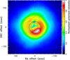 |
Fig. 17 Comparison between the continuum-subtracted integrated intensity map of the 267.93 GHz AlO line (contours) and the polarized intensity map (color map) obtained at 820 nm. The AlO intensity map was obtained by integrating across a velocity range from Vrel = −36 to 36 km s−1. The black circle represents the millimeter continuum diameter. The gray contours correspond to 0.045 (3σ), 0.15 (10σ), 0.3 (20σ), 0.45 (30σ), and 0.675 (45σ) mJy/beam km s−1, while the white contours correspond to −0.15 (−10σ) and −0.045 (−3σ) mJy/beam km s−1. The polarized intensity is normalized to 1 at its maximum. |
4.14 TiO and TiO2
The TiO and TiO2 molecules are considered to be potentially important for dust formation, because they can provide nucleation seeds, on which other grain species can grow. We detect a vibrationally excited TiO line (v = 1, 3Δ1, J = 8–7, Eu = 1492 K) at 251.802917 GHz, a 50TiO line (v = 0, 3Δ2, J = 8–7, Eu = 192 K) at 253.591920 GHz, and a 49TiO line (v = 0, 3Δ1, J = 8–7, Eu = 53 K) at 251.957928 GHz. Figure F.1 shows the channel maps for the TiO v = 1 line at 251.802917 GHz, which overlaps with the AlOH line described above at Vrel ≳ 6 km s−1. The emission is ring-like just outside the limb of the stellar disk, extending only to ~40 mas (1.3 Rcont = 1.9 R⋆). Enhanced emission can be seen in the NNW and SE (Vrel = +1.5 to +3.0 km s−1) as well as in the SW (Vrel = −3 to 0.0 km s−1). The channel maps of the 50TiO line, shown in Fig. F.2, are of a lower S/N ratio of ~5. Nevertheless, it can be recognized that the emission features are located along or just outside the limb of the stellar disk. The channel maps of the 49TiO line are of even lower S/N, and therefore, we only present the integrated intensity map in Fig. F.3 for completeness.
TiO emission has been observed at a much greater radius in the visible. The continuum-subtracted image of W Hya obtained at 717 nm (Ohnaka et al. 2017), corresponding to the γ bands of the TiO’s electronic transition, shows emission extending to 100–150 mas about four years prior to the ALMA observations. Our TiO v = 1 emission is compact because the transition probability is much smaller than those of the γ bands in the visible.
Figure 18 shows a comparison of the integrated intensity maps of the TiO line and the AlO N = 7–6 line. The positions of the enhanced TiO emission agree very well with that of the AlO line with the three major emission clumps in the east, SW, and NNW, although the extended NNW plume is absent in the TiO line. Figure 19 shows a comparison of the TiO integrated intensity map and the polarized intensity map at 820 nm reported in Paper I. The TiO emission overlaps well with the scattered light from the clumpy dust clouds. We discuss the interpretation of the overlap in Sect. 5, together with other molecular lines.
We detect five TiO2 lines. While the emission is not sufficiently strong to be seen in the channel maps, the integrated intensity maps confirm the detection as shown in Fig. F.4. The image of the TiO2 line #54 at 251.708056 GHz (Fig. F.4a) shows the emission most clearly. It extends up to ~100 mas (4.8 R⋆) in the north and east. The line #51 also shows emission to ~80 mas, although the emission is less clear. This shows that TiO2 is not entirely lock up in dust grains up to 4–5 R⋆. The other TiO2 lines show emission just outside the limb of the stellar disk due to their higher excitation energies or a smaller Einstein coefficient.
We stacked the images of five detected TiO2 lines to better visualize the spatial distribution of TiO2. Figure F.5 shows a comparison of the stacked TiO2 image (color map) and the 251.80 GHz TiO line (contours). The TiO2 emission coincides rather well, if not perfectly, with the TiO image, with the most pronounced emission located in the east, SW, and NW. As discussed in Sect. 5, TiO2 is another molecular species, together with some other molecules, whose formation is enhanced in the regions where shock-induced chemistry is active and dust formation takes place.
Kamiński et al. (2017) detect TiO2 toward o Cet and find that the TiO2 emission extends to 2.7–5.5 R⋆, more extended than that of TiO (<4 R⋆). Decin et al. (2018) present similar results for R Dor and IK Tau. The observed extension of the TiO2 lines in W Hya is in qualitative agreement with these results. However, we cannot conclude that the abundance distribution of TiO2 is more extended than that of TiO from our data alone, owing to the differences in the excitation energies.
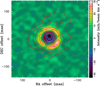 |
Fig. 18 Comparison of the continuum-subtracted integrated intensity maps of the lines of TiO (v = 1, 3Δ1, J = 8–7) and AlO (N = 7–6). The color map and contours represent the TiO and AlO lines, respectively. The TiO intensity map was obtained by integrating from Vrel = −10 to 6 km s−1, avoiding the AlOH line. The red and light blue contours correspond to the same positive and negative intensity levels, respectively, as shown in Fig. 17. |
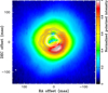 |
Fig. 19 Comparison of the continuum-subtracted integrated intensity maps of the vibrationally excited TiO line (v = 1, 3Δ1, J = 8–7) and the polarized intensity map obtained at 820 nm. The color map and contours represent the polarized intensity and the TiO line, respectively. The gray and white contours correspond to positive values (0.01, 0.015, 0.02, and 0.025 mJy/beam km s−1) and negative values (−0.025, −0.02, −0.015, and −0.01 mJy/beam km s−1), respectively. |
4.15 High excitation OH lines
We detect two OH lines (v = 0, Nj = 1835/2, F = 18+−18− and F = 17+−17−) at 265.734659 and 265.765323 GHz, which correspond to the Λ-doubling hyperfine components. Because the S/N ratios of the individual channel maps are quite low, we present in Fig. G.1 the intensity maps integrated from Vrel = −10 to 10 km s−1. Due to their high upper level energy of 8860 K, these OH lines form in layers close to the star, resulting in the compact emission. The figure shows that the emission is seen in the north and SW along the limb of the stellar disk. Interestingly, while the northern emission is seen just outside the stellar limb, the SW emission is detected on and inside the limb.
Khouri et al. (2019) report the detection of the Λ-doubling of high excitation OH lines from 107 to 352 GHz in three AGB stars, W Hya, R Dor, and IK Tau, including the same 266 GHz pair toward W Hya taken at a lower angular resolution of ~110×190 mas on 2017 July 8 (phase 0.74). Their analysis of the OH lines with Eu spanning from 4818 to 12756 K shows a rotational temperature of 2472 ± 184 K for the emission within a radius of 44 mas. The temperature is comparable to the continuum brightness temperatures of 2500–2650 K that they obtained, which can explain the OH emission seen close to the star in our images. Baudry et al. (2023) detect one of the hyperfine components (F = 18+−18−) only in R Hya and tentatively in Mira (o Cet) among their sample of 17 AGB stars and RSGs.
Khouri et al. (2019) also present high-angular resolution images of W Hya in Band 4 OH lines at ~130 GHz with a restoring beam of ~30 mas and detect emission partially over the stellar disk. Our images obtained at a higher angular resolution reveal that the emission is primarily located along the limb of the stellar disk. Based on the observed flux ratio of the Λ-doubling lines, Khouri et al. (2019) suggest possible maser action in the OH lines at 265.7 GHz. While the weak OH emission over the stellar disk detected in our data may also be masers, we need data with higher S/N to confirm this possibility.
4.16 Unidentified lines
There are seven lines that could not be identified. Figures H.1, H.2, H.3, and H.4 show the channel maps obtained for U253913, U250652, U252586, and U266902, respectively. The rest frequency of U253913 is close to the vibrationally excited SO2 line v2 = 2 v3 = 1293,26−292,27 at 253.915158 GHz listed in HITRAN. However, its excitation energy Eu = 3867 K seems to be too high, and the frequency is also uncertain (H. Müller, priv. comm.). Therefore, we do not identify the line as SO2 but mark is as unidentified.
In the cases of U250652 and U252586, emission is clearly seen in the east just off the limb of the stellar disk at Vrel = −1.5 and 0 km s−1. The positions of the emission as well as its velocities are similar to that of the AlOH line discussed in Sect. 4.13, although no AlOH line is present in the list of Splatalogue, CDMS, JPL, and HITRAN. In the case of U266902, we note that a weak, unidentified line at the same rest frequency is also detected in VX Sgr among a sample of 17 O-rich AGB stars and RSGs (Wallström et al. 2024). U266902 is close to a direct ℓ-type transition of H13CN line at 266.904987 GHz (v2 = 1, J = 35, l = 1e−1f). However, its Einstein coefficient is very small (log Aul = −5.818), and its upper level energy is relatively high (Eu = 3632 K). As shown in Fig. D.1, the vibrationally excited HCN line appears very weak in spite of its larger Einstein coefficient (log Aul = −3.142), lower upper level energy (Eu = 1050 K), and its status as the main isotopologue (i.e., H12CN). Furthermore, direct l-type HCN transitions in carbon stars have only been found in the main isotopologue (Thorwirth et al. 2003; Cernicharo et al. 2011). Therefore, it is unlikely that U266902 is due to H13CN.
For U250797, U253724, and U268099, we only show the integrated intensity maps in Fig. H.5, because the individual channel maps are of low S/N ratios. We find lines due to AlS (250.802235 GHz) and 17OH (250.796230 GHz) near U250797. However, we detect no signatures of another AlS line at 250.841643 GHz with approximately the same upper level energy and Einstein coefficient. Neither did we see a trace of two AlS lines at 250.930853 and 250.936712 GHz with higher Einstein coefficients. Therefore, we deem the identification as AlS to be unlikely. The 17OH line has a very small Einstein coefficient of log Aul = −7.981, which also makes it unlikely to be the identification of U250797.
For U268099 and U253724, we find SO18O lines at nearby frequencies: v = 0,244,21−251,24 at 268.0964242 GHz listed in the CDMS catalog for U268099 and v2 = 1, 278,19−287,22 at 253.723621 GHz listed in HITRAN for U253724. However, while there are a number of ground-state SO18O lines in the observed spectral windows, none of them is detected. Therefore, the identification of U268099 and U253724 as SO18O is unlikely. Another candidate for U268099 is the vibrationally excited SO2 line (v2 = 2,329,23−338.26, Eu = 729 K) at 268.106284 GHz listed in HITRAN. The rest frequency is blueshifted by 8.1 km s−1 with respect to the observed line. Given that the uncertainty in the frequency of vibrationally excited transitions is often large, and the velocity shift is caused by the atmospheric dynamics, we cannot exclude this line for the identification of U268099.
5 Discussion
In Paper I, we find striking agreement between the spatial distributions of the clumpy dust clouds seen in the 820 nm polarized intensity map and the nonthermal, likely maser emission of the vibrationally excited H2O line (v2 = 265,2−74,3) at 268 GHz. In the complete data reported in the present paper, we reveal similar good agreement between the dust clouds distribution and the lines of AlO (Fig. 17) and TiO (Fig. 19). The emission of the vibrationally excited HCN line (v2 = 11e) also overlaps with the signals of the dust clouds but extends farther out. Figure I.1 shows that the emission of more molecular lines coincides with the dust clouds: 30SiO (v = 1, line #4), Si17O (v = 0, line #5), TiO2 (stacked image of lines #51–#55, Sect. 4.14), SO (v = 0, NJ = 65−54, line #41), and two SO2 lines (lines #9 and #20). The emission of more SO2 lines shows noticeable overlap with the dust clouds, and two lines are presented as examples. The emission of these lines traces the paisley-like dust cloud in the SW quadrant, another cloud with moderate signals in the east, and the weaker dust signals in the NNW plume.
The observed overlap between the dust clouds and molecular line emission indicates not only AlO and TiO but also some other molecules are involved in the chemical network including dust formation. We propose in Paper I that the 268 GHz H2O emission and dust both trace cool, dense pockets. Moreover, H2O is an important oxidizing agent for the formation of a number of molecules and molecular clusters that are precursors of dust, and SiO also plays an important role in these chemical reactions (Goumans & Bromley 2012; Gobrecht et al. 2016; Andersson et al. 2023). AlO is also considered to be important as a precursor of seed particles (Gobrecht et al. 2022). Therefore, the agreement between the emission of H2O, SiO, and AlO and the dust clouds can be interpreted as that these molecules directly take part in the chemical network leading to dust formation.
An alternative interpretation of the overlap of these molecular species with dust emission is that their formation may be favored in regions where the dust is located. Examples of these regions include dense pockets created by convection and/or pulsation. For example, it is possible that some Si is processed back to the gas phase from the dust grains and forms the SiO molecule. As discussed in Sect. 4.5, the present data do not provide tight constraints on the Si abundance in the gas phase, and multiline observations including 28SiO are needed to address this point.
Gobrecht et al. (2016) also show that there are molecules that form in post-shock gas-phase chemistry but are not directly associated with grain nucleation. SO and SO2, which forms from SO, are among such molecules. In general, sulfur is not significantly depleted onto dust grains (Danilovich et al. 2020 and references therein). On the other hand, grain nucleation also starts behind shock fronts, where the density is enhanced (e.g., Liljegren et al. 2017). Therefore, the observed agreement between the SO and SO2 emission and dust clouds lends support to the idea that the formation of these molecular species and dust grains is both associated with shocks in the same localized regions. As discussed in Sect. 4.12, HCN also likely forms in shock-induced chemistry, and the spatial distribution of the HCN v2 = 11e emission indeed covers the dust cloud formation regions. However, the HCN emission is much more extended than the dust clouds, suggesting that this molecular species is not actively involved in or depleted by grain formation. The differences in the distribution of SO2/SO and HCN may be due to the differences in their formation reactions and excitation, which depend on the ambient conditions.
While TiO2 is also considered to be a precursor of dust (Gail & Sedlmayr 1998; Jeong et al. 2003), the recent observations do not confirm its importance in dust formation (Kamiński et al. 2017; Decin et al. 2018). The shock-chemistry models of Gobrecht et al. (2016) also show that only a modest amount of TiO2 can form from TiO in shocks and conclude that TiO2 does not play an important role as seed particles. Therefore, the agreement of the TiO and TiO2 emission with the dust clouds does not necessarily indicate that these molecules actively participate in grain nucleation but that they form in shock-induced chemistry in the same localized regions as the dust clouds, as in the cases of SO and SO2.
The infall within ~2.5 Rcont (~3.6 R⋆) derived from the SiO lines (Sect. 4.5) and inferred from the 268 GHz H2O line (Paper I) means that the dust grains are forming in the infalling material if we assume that the gas and dust grains are kinematically coupled. As we point out in Paper I, this picture agrees with the 1D dynamical models, which show that shocks develop where the infalling material collides with the upwelling gas, and dust formation takes place behind shocks, where the density is enhanced (see Fig. 5 of Liljegren et al. 2017). As discussed in Sect. 4.5, the velocity profile derived from our modeling is consistent with this picture. The recent 3D models (Freytag & Höfner 2023) also show that there are dust clouds infalling up to ~25 km s−1, because the grain size is not large enough for the radiation pressure to accelerate the clouds outward. The observed infall velocities are within the prediction of the 3D models.
6 Conclusions
We identify 57 spectral lines of SiO, H2O, SO2, AlO, AlOH, TiO, TiO2, OH, SO, and HCN as well as their isotopologues in W Hya between 250 and 268 GHz. The angular resolution of ~20 mas of our ALMA data and the large angular size of W Hya of ~60 mas in the millimeter continuum enable us to spatially resolve the stellar disk and atmosphere within several stellar radii. We detect a plume in the NNW and a tail-like structure in the SSW, both extending to ~100 mas (~4.8 R⋆). The atmosphere is elongated in the ENE-WSW direction with semimajor and semiminor axes of ~70 and ~40 mas, respectively.
About 2/3 of the identified lines appear in absorption over the stellar disk as expected for thermal excitation. The absorption is inhomogeneous over the stellar disk. However, about 1/3 of the identified lines – some lines of SiO, H2O, SO2, and AlO – show emission on top of the continuum over the stellar disk, which cannot be explained by material warmer than the millimeter continuum-forming layer. This indicates nonthermal emission – either suprathermal emission or maser action. Particularly, we detect clear maser emission from the 29SiO line (v = 2, J = 6–5), in addition to the likely maser emission of the vibrationally excited H2O line at 268 GHz (v2 = 2, JKa,Kc = 65,2−74,3) over the stellar disk reported in Paper I. The emission over the stellar disk complicates the interpretation of the data in terms of kinematics. Nevertheless, our modeling of two SiO lines without signatures of nonthermal emission suggests an accelerating infall toward the continuum-forming layer, from ~0 km s−1 at ~75 mas (~3.6 R⋆) to ~11 km s−1 at ~50 mas (~2.4 R⋆), and outflow at up to 10 km s−1 in deeper layers. The dynamics in this region are dominated by the pulsation and/or convection; they remain gravitationally bound, and the material is not yet outflowing in a stationary wind. A detailed non-LTE analysis is needed to derive the abundances of the different molecular species, which will allow us to better understand the chemical processes involving molecules and dust as well as their interplay with stellar pulsation and convection.
The emission of the SiO and AlO lines as well as the 268 GHz H2O line from Paper I shows noticeable agreement with the spatial distribution of the clumpy dust clouds seen in the visible polarimetric images contemporaneously taken with our ALMA data. This is consistent with the chemical models that directly associate SiO, H2O, and AlO with the grain nucleation process. On the other hand, the overlap of the SO and SO2 emission with the dust clouds implies that these molecular species and dust form behind shock fronts, even though SO and SO2 are not expected to be associated with dust formation. This can also be the case for TiO and TiO2.
We detect the vibrationally excited HCN line emission very close to the star, down to the millimeter continuum radius of ~30 mas (~1.4 R⋆). The HCN emission overlaps with the dust clouds but it is more extended, which implies that the inner HCN is likely produced by shock-induced chemistry but not actively involved in dust formation.
The emission of the HCN (v = 0, J = 3–2) and SO (NJ = 65−54) lines is much more extended up to ~1″. We detect the filamentary, spider-like structures, which likely correspond to localized regions with high intensities. However, diffuse, smooth emission on scales larger than ~190 mas is missing due to the lack of short baselines, which prevented us from drawing a conclusion on the large-scale kinematics. This issue can only be solved with observations combining ALMA’s extended and compact configurations, preferably simultaneously, given the variabilities in line intensities and spatial distributions. As discussed above, it is also important to carry out high-resolution observations at other variability phases to understand the phase dependence of the molecular emission in the inner winds, which will be tested against chemical and hydrodynamical models. A frequent access to both long and short baselines (on a timescale of months) is essential; this is currently unavailable but may be considered for a future upgrade of ALMA.
Data availability
The figures in Appendices are available on Zenodo zenodo.org/records/17118092.
Acknowledgements
This paper makes use of the following ALMA data: ADS/JAO.ALMA#2018.1.01239.S. ALMA is a partnership of ESO (representing its member states), NSF (USA) and NINS (Japan), together with NRC (Canada), NSTC and ASIAA (Taiwan), and KASI (Republic of Korea), in cooperation with the Republic of Chile. The Joint ALMA Observatory is operated by ESO, AUI/NRAO and NAOJ. Data reduction was carried out at the IRAM ARC node. We are grateful to Holger Müller for the discussion about the line identification. We also thank the anonymous referee, whose careful and constructive comments helped us improve the manuscript. K.O. acknowledges the support of the Agencia Nacional de Investigación Científica y Desarrollo (ANID) through the FONDECYT Regular grant 1240301. K.T.W. acknowledges support from the European Research Council (ERC) under the European Union’s Horizon 2020 research and innovation programme (Grant agreement no. 883867, project EXWINGS). This research made use of the SIMBAD database, operated at the CDS, Strasbourg, France.
References
- Adam, C., & Ohnaka, K. 2019, A&A, 628, A132 [NASA ADS] [CrossRef] [EDP Sciences] [Google Scholar]
- Agúndez, M., Cernicharo, J., & Guélin, M. 2010, ApJ, 724, L133 [CrossRef] [Google Scholar]
- Agúndez, M., Martínez, J. I., de Andres, P. L., Cernicharo, J., & Martín-Gago, J. A. 2020, A&A, 637, A59 [Google Scholar]
- Ahrens, V., Lewen, F., Takano, S., et al. 2002, Z. Naturfor. A, 57, 669 [NASA ADS] [CrossRef] [Google Scholar]
- Andersson, S. Gobrecht, D., & Valero, R. 2023, Front. Astron. Space Sci., 10, 52 [Google Scholar]
- Andriantsaralaza, M., Ramstedt, S., Vlemmings, W. H. T., & De Beck, E. 2022, A&A, 667, A74 [NASA ADS] [CrossRef] [EDP Sciences] [Google Scholar]
- Asaki, Y., Maud, L. T., Francke, H., et al. 2023, ApJ, 958, 86 [NASA ADS] [Google Scholar]
- Baudry, A., Wong, K. T., Etoka, S., et al. 2023, A&A, 674, A125 [NASA ADS] [CrossRef] [EDP Sciences] [Google Scholar]
- Bladh, S., Liljegren, S., Höfner, S., Aringer, B., & Marigo, P. 2019, A&A, 626, A100 [NASA ADS] [CrossRef] [EDP Sciences] [Google Scholar]
- Bojnordi Arbab, B., Vlemmings, W., Khouri, T., & Höfner, S. 2024, ApJ, 976, 138 [Google Scholar]
- CASA Team (Bean, B., et al.) 2022, PASP, 134, 114501 [NASA ADS] [CrossRef] [Google Scholar]
- Cernicharo, J., & Bujarrabal, V. 1992, ApJ, 401, L109 [Google Scholar]
- Cernicharo, J., Agúndez, M., Kahane, C., et al. 2011, A&A, 529, L3 [NASA ADS] [CrossRef] [EDP Sciences] [Google Scholar]
- Charnley, S. B., Tielens, A. G. G. M., & Kress, M. E. 1995, MNRAS, 274, L53 [NASA ADS] [CrossRef] [Google Scholar]
- Cortes, P. C., Carpenter, J., Kameno, S., et al. 2025, ALMA Technical Handbook, ALMA Doc. 12.3, ver. 1.5 [Google Scholar]
- Cornwell, T. J. 2008, IEEE J. Selected Top. Signal Process., 2, 793 [NASA ADS] [CrossRef] [Google Scholar]
- Danilovich, T., de Beck, E., Black, J. H., Olofsson, & Justtanont, K. 2016, A&A, 588, A119 [NASA ADS] [CrossRef] [EDP Sciences] [Google Scholar]
- Danilovich, T., Decin, L., Karakas, A., et al. 2017, A&A, 602, A14 [NASA ADS] [CrossRef] [EDP Sciences] [Google Scholar]
- Danilovich, T., Richards, A. M. S., Decin, L., Van de Sande, M., & Gottlieb, C. A. 2020, MNRAS, 494, 1323 [NASA ADS] [CrossRef] [Google Scholar]
- De Beck, E., & Olofsson, H. 2018, A&A, 615, A8 [NASA ADS] [CrossRef] [EDP Sciences] [Google Scholar]
- Decin, L., De Beck, E., Brünken, S., et al. 2010, A&A, 516, A69 [NASA ADS] [CrossRef] [EDP Sciences] [Google Scholar]
- Decin, L., Richards, A. M. S., Waters, L. B. F. M., et al. 2017, A&A, 608, A55 [NASA ADS] [CrossRef] [EDP Sciences] [Google Scholar]
- Decin, L., Richards, A. M. S., Danilovich, T., Homan, W., & Nuth, J. A. 2018, A&A, 615, A28 [NASA ADS] [CrossRef] [EDP Sciences] [Google Scholar]
- Decin, L., Montargès, M., Richards, A. M. S., et al. 2020, Science, 369, 1497 [Google Scholar]
- Dehaes, S., Groenewegen, M. A. T., Decin, L., et al. 2007, MNRAS, 377, 931 [NASA ADS] [CrossRef] [Google Scholar]
- Deshmukh, S. A., Ludwig, H.-G., Kučinskas, A., et al. 2022, A&A, 668, A48 [NASA ADS] [CrossRef] [EDP Sciences] [Google Scholar]
- Drevon, J., Millour, F., Cruzalèbes, P., et al. 2022, A&A, 665, A32 [NASA ADS] [CrossRef] [EDP Sciences] [Google Scholar]
- Endres, C. P., Schlemmer, S., Schilke, P., Stutzki, J., & Müller, H. S. P. 2016, J. Mol. Spectrosc., 327, 95 [NASA ADS] [CrossRef] [Google Scholar]
- Freytag, B., & Höfner, S. 2023, A&A, 669, A155 [NASA ADS] [CrossRef] [EDP Sciences] [Google Scholar]
- Furtenbacher, T., Tóbiás, R., Tennyson, J., Polyansky, O. L., & Császár, A. G. 2020a, J. Phys. Chem. Ref. Data, 49, 033101 [NASA ADS] [CrossRef] [Google Scholar]
- Furtenbacher, T., Tóbiás, R., Tennyson, J., et al. 2020b, J. Phys. Chem. Ref. Data, 49, 043103 [NASA ADS] [CrossRef] [Google Scholar]
- Gail, H-P., & Sedlmayr, E. 1998, Faraday Discuss, 109, 303 [Google Scholar]
- Gobrecht, D., Cherchneff, I., Sarangi, A., Plane, J. M. C., & Bromley, S. T. 2016, A&A, 585, A6 [NASA ADS] [CrossRef] [EDP Sciences] [Google Scholar]
- Gobrecht, D., Plane, J. M. C., Bromley, S. T., et al. 2022, A&A, 658, A167 [NASA ADS] [CrossRef] [EDP Sciences] [Google Scholar]
- Goldsmith, P. F., & Langer, W. D. 1999, ApJ, 517, 209 [Google Scholar]
- Gordon, I. E., Rothman, L. S., & Hargreaves, R. J. 2022, J. Quant. Spectrosc. Radiat. Transfer, 277, 107949 [NASA ADS] [CrossRef] [Google Scholar]
- Gottlieb, C. A., Decin, L., Richards, A. M. S., et al. 2022, A&A, 660, A94 [CrossRef] [EDP Sciences] [Google Scholar]
- Goumans, T. P. M., & Bromley, S. T. 2012, MNRAS, 420, 3344 [NASA ADS] [Google Scholar]
- Gray, M. D., Baudry, A., Richards, A. M. S., et al. 2016, MNRAS, 456, 374 [NASA ADS] [CrossRef] [Google Scholar]
- Herpin, F., & Baudry, A. 2000, A&A, 359, 1117 [NASA ADS] [Google Scholar]
- Hoai, D. T., Nhung, P. T., Darriulat, P., et al. 2022, Vietnam J. Sci. Technol. Eng., 64, 16 [CrossRef] [Google Scholar]
- Höfner, S., & Freytag, B. 2019, A&A, 623, A158 [NASA ADS] [CrossRef] [EDP Sciences] [Google Scholar]
- Höfner, S., & Olofsson, H. 2018, A&ARv, 26, 1 [Google Scholar]
- Höfner, S., Bladh, S., Aringer, B., & Ahuja, R. 2016, A&A, 594, A108 [NASA ADS] [CrossRef] [EDP Sciences] [Google Scholar]
- Höfner, S., Bladh, S., Aringer, B., & Eriksson, K. 2022, A&A, 657, A109 [NASA ADS] [CrossRef] [EDP Sciences] [Google Scholar]
- Humphreys, E. M. L., Gray, M. D., Yates, J. A., et al. 2002, A&A, 386, 256 [NASA ADS] [CrossRef] [EDP Sciences] [Google Scholar]
- Imai, H., Nakashima, J., Deguchi, S., et al. 2010, PASJ, 62, 431 [Google Scholar]
- Ireland, M. J., Tuthill, P. G., Davis, J., & Tango, W. 2005, MNRAS, 361, 337 [CrossRef] [Google Scholar]
- Jeong, K. S., Winters, J. M., Le Bertre, T., & Sedlmayr, E. 2003, A&A, 407, 191 [NASA ADS] [CrossRef] [EDP Sciences] [Google Scholar]
- Jäger, C., Dorschner, J., Mutschke, H., Posch, T., & Henning, Th. 2003, A&A, 408, 193 [NASA ADS] [CrossRef] [EDP Sciences] [Google Scholar]
- Kamiński, T. 2019, Proc. IAU Symp., 343, 108 [Google Scholar]
- Kamiński, T., Wong, K. T., Schmidt, M. R., et al. 2016, A&A, 592, A42 [NASA ADS] [CrossRef] [EDP Sciences] [Google Scholar]
- Kamiński, T., Müller, H. S. P., Schmidt, M. R., et al. 2017, A&A, 599, A59 [NASA ADS] [CrossRef] [EDP Sciences] [Google Scholar]
- Khouri, T., de Koter, A., Decin, L., et al. 2014a, A&A, 561, A5 [NASA ADS] [CrossRef] [EDP Sciences] [Google Scholar]
- Khouri, T., de Koter, A., Decin, L., et al. 2014b, A&A, 570, A67 [NASA ADS] [CrossRef] [EDP Sciences] [Google Scholar]
- Khouri, T., Waters, L. B. F. M., de Koter, A., et al. 2015, A&A, 577, A114 [NASA ADS] [CrossRef] [EDP Sciences] [Google Scholar]
- Khouri, T., Maercker, M., Waters, L. B. F. M., et al. 2016, A&A, 591, A70 [NASA ADS] [CrossRef] [EDP Sciences] [Google Scholar]
- Khouri, T., Vlemmings, W. H. T., Olofsson, H., et al. 2018, A&A, 620, A75 [NASA ADS] [CrossRef] [EDP Sciences] [Google Scholar]
- Khouri, T., Velilla-Prieto, L., De Beck, E., et al. 2019, A&A, 623, L1 [NASA ADS] [CrossRef] [EDP Sciences] [Google Scholar]
- Khouri, T., Olofsson, H., Vlemmings, W. H. T., et al. 2024, A&A, 685, A11 [NASA ADS] [CrossRef] [EDP Sciences] [Google Scholar]
- Knapp, G. R., Pourbaix, D., Platais, I., & Jorissen, A. 2003, A&A, 403, 993 [NASA ADS] [CrossRef] [EDP Sciences] [Google Scholar]
- Lanquetin, R., Coudert, L. H., & Camy-Peyret, C. 2001, J. Mol. Spectrosc., 206, 83 [Google Scholar]
- Lebzelter, T., Hinkle, K. H., & Aringer, B. 2001, A&A, 377, 617 [NASA ADS] [CrossRef] [EDP Sciences] [Google Scholar]
- Liljegren, S., Höfner, S., Eriksson, K., & Nowotny, W. 2017, A&A, 606, A6 [NASA ADS] [CrossRef] [EDP Sciences] [Google Scholar]
- Maercker, M., Mohamed, S., Vlemmings, W. H. T., et al. 2012, Nature, 490, 232 [NASA ADS] [CrossRef] [Google Scholar]
- Martí-Vidal, I., Vlemmings, W. H. T., Muller, S., & Casey, S. 2014, A&A, 563, A136 [Google Scholar]
- Matthews, L. D., Reid, M. J., & Menten, K. M. 2015, ApJ, 808, 36 [Google Scholar]
- Mihalas, D. 1978, Stellar Atmospheres, 2nd edn. (San Francisco: W. H. Freeman and Co.) [Google Scholar]
- Müller, S., Dinh-V-Trung, He, J.-H., & Lim, J. 2008, ApJ, 684, L33 [NASA ADS] [CrossRef] [Google Scholar]
- Müller, H. S. P., Thorwirth, S., Roth, D. A., & Winnewisser, G. 2001, A&A, 370, L49 [Google Scholar]
- Müller, H. S. P., Schlöder, F., Stutzki, J., & Winnewisser, G. 2005, J. Mol. Struct., 742, 215 [Google Scholar]
- Norris, B., Tuthill, P. G., Ireland, M. J., et al. 2012, Nature, 484, 220 [NASA ADS] [CrossRef] [Google Scholar]
- Nowotny, W., Höfner, S., & Aringer, B. 2010, A&A, 514, A35 [NASA ADS] [CrossRef] [EDP Sciences] [Google Scholar]
- Ohnaka, K., Weigelt, G., & Hofmann, K.-H. 2016, A&A, 589, A91 [NASA ADS] [CrossRef] [EDP Sciences] [Google Scholar]
- Ohnaka, K., Weigelt, G., & Hofmann, K.-H. 2017, A&A, 597, A20 [NASA ADS] [CrossRef] [EDP Sciences] [Google Scholar]
- Ohnaka, K., Weigelt, G., & Hofmann, K.-H. 2019, ApJ, 883, 89 [NASA ADS] [CrossRef] [Google Scholar]
- Ohnaka, K., Wong, K. T., Weigelt, G., & Hofmann, K.-H. 2024, A&A, 691, L14 [NASA ADS] [CrossRef] [EDP Sciences] [Google Scholar]
- Paladini, C., Baron, F., Jorissen, A., et al. 2018, Nature, 310, 553 [Google Scholar]
- Pearson, J. C., Anderson, T., Herbst, E., De Lucia, F. C., & Helminger, P. 1991, ApJ, 379, L41 [NASA ADS] [CrossRef] [Google Scholar]
- Peng, T.-C., Humphreys, E. M. L., Testi, L., et al. 2013, A&A, 559, L8 [NASA ADS] [CrossRef] [EDP Sciences] [Google Scholar]
- Pickett, H. M., Poynter, R. L., Cohen, E. A., et al. 1998, J. Quant. Spectrosc. & Radiat. Transfer, 60, 883 [Google Scholar]
- Planquart, L., Paladini, C., Jorissen, A., et al. 2024, A&A, 687, A306 [NASA ADS] [CrossRef] [EDP Sciences] [Google Scholar]
- Reid, M., J., & Menten, K. M. 1997, ApJ, 476, 327 [NASA ADS] [CrossRef] [Google Scholar]
- Reid, M., J., & Menten, K. M. 2007, ApJ, 671, 2068 [NASA ADS] [CrossRef] [Google Scholar]
- Siebert, M. A., Van de Sande, M., Millar, T. J., & Remijan, A. J. 2022, ApJ, 941, 90 [NASA ADS] [CrossRef] [Google Scholar]
- Takigawa, A., Kamizuka, T., Tachibana, S., & Yamamura, I. 2017, Sci. Adv., 3, eaao2149 [NASA ADS] [CrossRef] [Google Scholar]
- Thorwirth, S., Wyrowski, F., Schilke, P., et al. 2003, ApJ, 586, 338 [NASA ADS] [CrossRef] [Google Scholar]
- Tsuji, T., Ohnaka, K., Hinkle, K. H., & Ridgway, S. T. 1994, A&A, 289, 469 [NASA ADS] [Google Scholar]
- Uttenthaler, S., Van Stiphout, K., Voet, K., et al. 2011, A&A, 531, A88 [NASA ADS] [CrossRef] [EDP Sciences] [Google Scholar]
- Van de Sande, M., & Millar, T. J. 2019, ApJ, 873, 36 [CrossRef] [Google Scholar]
- Van de Sande, M., & Millar, T. J. 2022, MNRAS, 510, 1204 [Google Scholar]
- Van de Sande, M., Decin, L., Lombaert, R., et al. 2018, A&A, 609, A23 [Google Scholar]
- van Leeuwen, F. 2007, A&A, 474, 653 [CrossRef] [EDP Sciences] [Google Scholar]
- Velilla-Prieto, L., Fonfría, J. P., Agúndez, M., et al. 2023, Nature, 617, 696 [NASA ADS] [CrossRef] [Google Scholar]
- Vlemmings, W. H. T., van Langevelde, H. J., Diamond, P. J., Habing, H. J., & Schilizzi, R. T. 2003, A&A, 407, 213 [NASA ADS] [CrossRef] [EDP Sciences] [Google Scholar]
- Vlemmings, W. H. T., Humphreys, E. M. L., & Franco-Hernández, R. 2011, ApJ, 728, 149 [Google Scholar]
- Vlemmings, W., Khouri, T., O’Gorman, E., et al. 2017, Nat. Ast., 1, 848 [CrossRef] [Google Scholar]
- Vlemmings, W. H. T., Khouri, T., & Olofsson, H. 2019, A&A, 626, A81 [NASA ADS] [CrossRef] [EDP Sciences] [Google Scholar]
- Vlemmings, W. H. T., Khouri, T., & Tafoya, D. 2021, A&A, 654, A18 [NASA ADS] [CrossRef] [EDP Sciences] [Google Scholar]
- Vlemmings, W. H. T., Khouri, T., Bojnordi Arbab, B. De Beck, E., & Maercker, M. 2024, Nature, 633, 323 [Google Scholar]
- Wallström, S. H. J., Danilovich, T., Müller, H. S. P., et al. 2024, A&A, 681, A50 [NASA ADS] [CrossRef] [EDP Sciences] [Google Scholar]
- Wittkowski, M., Hofmann, K.-H., Höfner, S., et al. 2017, A&A, 601, A3 [NASA ADS] [CrossRef] [EDP Sciences] [Google Scholar]
- Wong, K. T., Kamiński, T., Menten, K. M., & Wyrowski, F., 2016, A&A, 590, A127 [NASA ADS] [CrossRef] [EDP Sciences] [Google Scholar]
- Yu, S., Pearson, J. C., Drouin, B. J., et al. 2012, J. Mol. Spectrosc., 279, 16 [NASA ADS] [CrossRef] [Google Scholar]
- Zhao-Geisler, R., Quirrenbach, A., Köhler, R., Lopez, B., & Leinert, C. 2011, A&A, 530, A120 [NASA ADS] [CrossRef] [EDP Sciences] [Google Scholar]
The reason for the difference in the results between Knapp et al. (2003) and Andriantsaralaza et al. (2022) is that the period-luminosity relation for semiregular variables is not tight, showing large scatter. This means that the distance derived from the fitted period-luminosity relation has significant uncertainty, and therefore, the result of Andriantsaralaza et al. (2022) deviates from the value directly derived from the Hipparcos parallax of W Hya itself (Knapp et al. 2003).
Paper I mistakenly mentions that Vlemmings et al. (2021) interpreted the CO v = 1 J = 3–2 as masers. It is the CO v = 0 J = 3–2 line that Vlemmings et al. (2021) present as maser emission.
Because the pressure and temperature profiles are shown only to 10 R⋆ in Agúndez et al. (2020), we extrapolated up to 150 R⋆ with power-law decreases.
We note that the grainy appearance of the maps near the systemic velocity is a result of nonuniform emission and missing short spacings that introduce artifacts on the size scales adopted in the CLEAN process.
If there were contribution from the much weaker hyperfine components F = 3–3 and 2–2, they would appear at velocity shifts of 1.7 and −2.4 km s−1 with respect to the main components at Vrel = −5 km s−1, respectively, i.e., at Vrel = −3.3 and −7.4 km s−1. However, there is no signature of absorption at these velocities. The contributions from the weaker hyperfine components are therefore insignificant.
All Tables
Upper and lower level energies and the rest frequency of the H2O v2 = 292,8−83,5 line from different databases.
All Figures
|
Fig. 1 Continuum-subtracted maps of W Hya observed at the systemic velocity in the different molecular lines presented in the main text. The images of two H2O lines (#6 and #7) are from Paper I. The color scale shown above each panel corresponds to mJy/beam except for #3, where it is given in Jy/beam. The black circles represent the ellipse fit to the continuum image. The identification number of each line in Table 2 is shown in the upper left corner. The restoring beam size is shown in the lower left corner of each panel. North is up, and east is to the left. |
| In the text | |
|
Fig. 2 Continuum spectrum of W Hya at 250–268 GHz. The black dots represent the observed continuum fluxes, while the solid red line represents a power-law fit with Fv ∝ v2.08. The horizontal bars show the bandwidth of the spectral windows, not errors. |
| In the text | |
|
Fig. 3 Continuum-subtracted channel maps of W Hya observed in the 29SiO v = 3 J = 6–5 line at 251.930123 GHz. The black circles represent the ellipse fit to the continuum image. In the upper left corner of each panel, the LSR velocity and the relative velocity Vrel = VLSR − Vsys, Vsys = 40.4 km s−1 are shown. The restoring beam size is shown in the lower left corner of each panel. North is up, and east is to the left. |
| In the text | |
|
Fig. 4 Spatially resolved spectra of four SiO lines detected in our ALMA observations. (a) Continuum-subtracted intensity map of the Si 17O line (v = 0, J = 6–5) integrated from Vrel = −10 to 10 km s−1. The crosses and numbers represent the positions where the spatially resolved spectra shown in panels b–p were derived. (b–f) Spatially resolved spectra observed at five positions over the stellar disk. The black, red, green, and blue lines represent the spectra of the 29SiO v = 3 J = 6–5, 30SiO v = 2 J = 6–5, 30SiO v = 1 J = 6–5, and Si17O v = 0 J = 6–5 lines, respectively. The spectra were obtained from the data cube with the continuum emission. (g–k) SiO spectra obtained at positions 5–8 at a radial distance of 50 mas from the stellar disk center. These spectra were extracted from the continuum-subtracted data cube. The spectra measured at the disk center are shown in panel g to facilitate comparison between the absorption and emission spectra. (l–p) SiO spectra obtained at positions 9–12 at a radial distance of 90 mas from the stellar disk center, shown in the same manner as in panels g–k. |
| In the text | |
|
Fig. 5 Continuum-subtracted channel maps of W Hya obtained in the 30SiO v = 2 J = 6–5 line at 250.727751 GHz, shown in the same manner as Fig. 3. The maps at Vrel ≤ −10.5 km s−1 are severely affected by the Si17O line at 250.745 GHz (presented in Fig. 9). |
| In the text | |
|
Fig. 6 Continuum-subtracted channel maps of W Hya obtained in the 30SiO v = 1 J = 6–5 line at 252.471372 GHz, shown in the same manner as Fig. 3. |
| In the text | |
|
Fig. 7 Position-velocity diagram in the direction from PA = 45° to 225° obtained from the continuum-subtracted channel maps of the 30SiO line (v = 1, J = 6–5). The pink, red, and light blue curves at the negative spatial offsets (on the side of PA = 45°) represent the traces expected from shells infalling at velocities of 2 km s−1 at a radius of 75 mas, 7 km s−1 at 50 mas, and 13 km s−1 at 42 mas, respectively. The blue curve on the PA = 225° side shows the trace from an infalling or outflowing (although infalling is more plausible) shell with a velocity of 12 km s−1 at a radius of 45 mas. See Sect. 4.4. |
| In the text | |
|
Fig. 8 Spherical LTE model for the 30SiO v = 1 J = 6–5 and 29SiO v = 3 J = 6–5 lines. Panels a and b show a comparison between the model (black) and the spectra of the 30SiO v = 1 line (red) observed over the stellar disk and off the limb of the disk (positions 2 and 6 in Fig. 4), respectively. Panels c and d show a comparison for the 29SiO v = 3 line in the same manner. The velocity profile of the model is shown in panel e. Positive and negative velocities correspond to infall and outflow, respectively. Panel f shows the 29SiO number density (assumed to be equal to that of 30SiO) on the left ordinate and the gas temperature on the right ordinate. In panels e and f, the radius is shown in the units of Rcont (below) and R⋆ (above). |
| In the text | |
|
Fig. 9 Continuum-subtracted channel maps of W Hya obtained in the Si17O v = 0 J = 6–5 line at 250.744695 GHz, shown in the same manner as Fig. 3. The signals in the images at Vrel ≥ 9 km s−1 are due to the 30SiO v = 2 J = 6–5 line. |
| In the text | |
|
Fig. 10 Continuum-subtracted channel maps of W Hya obtained for the 29SiO v = 2 J = 6–5 line at 253.703469 GHz, shown in the same manner as Fig. 3, except that the unit of the color scale is different from other channel maps to show the strong maser emission and weaker emission over the stellar disk. |
| In the text | |
|
Fig. 11 Continuum-subtracted channel maps of W Hya obtained in the SO2 line (v = 0 JKa,Kc = 3610,26−379,29) at 250.816786 GHz, shown in the same manner as Fig. 3. |
| In the text | |
|
Fig. 12 Continuum-subtracted channel maps of W Hya obtained in the SO2 line (v = 0 JKa,Kc = 324,28−315,27) at 252.563893 GHz, shown in the same manner as Fig. 3. |
| In the text | |
|
Fig. 13 Population diagram for the SO2 lines without signatures of nonthermal emission in the innermost and intermediate regions defined as annular areas between 30 and 60 mas (~1 and 2 Rcont) and between 60 and 100 mas (~2 and 3.3 Rcont), respectively. The red and blue dots represent the measurements in the innermost and intermediate regions, respectively. The solid red and blue lines represent the fits in the respective regions. The excitation temperatures (Tex) and column densities (NSO2) derived in two regions are also shown. |
| In the text | |
|
Fig. 14 Continuum-subtracted channel maps of W Hya obtained in the SO line (v = 0, NJ = 65−54) at 251.825770 GHz, shown in the same manner as Fig. 3 but for a field of view of 550×550 mas. In addition, the insets show the enlarged view (80×80 mas) of the signal over the stellar disk. |
| In the text | |
|
Fig. 15 Channel maps of W Hya obtained in the HCN (v = 0, J = 3–2) line at 265.886434 GHz, shown in the same manner as Fig. 3 but in a larger field of view of 550×550 mas. The insets show the enlarged view (80×80 mas) of the signal over the stellar disk. |
| In the text | |
|
Fig. 16 Color map: intensity map of the HCN (v2 = 11e, J = 3–2) line at 265.852709 GHz integrated from Vrel = −10.5 to 10.5 km s−1. Contours: polarized intensity obtained at 820 nm contemporaneously with our ALMA observations (Paper I). The contours are drawn on a logarithmic scale at 10%, 17%, 30%, 52%, and 90% of the peak value. The black circle represents the millimeter continuum stellar disk. The beam size of the HCN intensity map is shown in the lower left corner. |
| In the text | |
|
Fig. 17 Comparison between the continuum-subtracted integrated intensity map of the 267.93 GHz AlO line (contours) and the polarized intensity map (color map) obtained at 820 nm. The AlO intensity map was obtained by integrating across a velocity range from Vrel = −36 to 36 km s−1. The black circle represents the millimeter continuum diameter. The gray contours correspond to 0.045 (3σ), 0.15 (10σ), 0.3 (20σ), 0.45 (30σ), and 0.675 (45σ) mJy/beam km s−1, while the white contours correspond to −0.15 (−10σ) and −0.045 (−3σ) mJy/beam km s−1. The polarized intensity is normalized to 1 at its maximum. |
| In the text | |
|
Fig. 18 Comparison of the continuum-subtracted integrated intensity maps of the lines of TiO (v = 1, 3Δ1, J = 8–7) and AlO (N = 7–6). The color map and contours represent the TiO and AlO lines, respectively. The TiO intensity map was obtained by integrating from Vrel = −10 to 6 km s−1, avoiding the AlOH line. The red and light blue contours correspond to the same positive and negative intensity levels, respectively, as shown in Fig. 17. |
| In the text | |
|
Fig. 19 Comparison of the continuum-subtracted integrated intensity maps of the vibrationally excited TiO line (v = 1, 3Δ1, J = 8–7) and the polarized intensity map obtained at 820 nm. The color map and contours represent the polarized intensity and the TiO line, respectively. The gray and white contours correspond to positive values (0.01, 0.015, 0.02, and 0.025 mJy/beam km s−1) and negative values (−0.025, −0.02, −0.015, and −0.01 mJy/beam km s−1), respectively. |
| In the text | |
Current usage metrics show cumulative count of Article Views (full-text article views including HTML views, PDF and ePub downloads, according to the available data) and Abstracts Views on Vision4Press platform.
Data correspond to usage on the plateform after 2015. The current usage metrics is available 48-96 hours after online publication and is updated daily on week days.
Initial download of the metrics may take a while.