| Issue |
A&A
Volume 704, December 2025
|
|
|---|---|---|
| Article Number | A122 | |
| Number of page(s) | 16 | |
| Section | Planets, planetary systems, and small bodies | |
| DOI | https://doi.org/10.1051/0004-6361/202555883 | |
| Published online | 09 December 2025 | |
Modeling of comet water production
II. Dust layer removal model: The case of 67P/Churyumov-Gerasimenko
1
Purple Mountain Observatory, Chinese Academy of Sciences,
Nanjing,
PR China
2
School of Astronomy and Space Science, University of Science and Technology of China,
Hefei
230026,
PR China
3
Max-Planck-Institut für Sonnensystemforschung,
Justus-von-Liebig-Weg 3,
37077
Göttingen,
Germany
4
Institut für Geophysik und extraterrestrische Physik, Technische Universität Braunschweig,
Mendelssohnstr. 3,
38106
Braunschweig,
Germany
5
European Space Agency (ESA), ESAC,
Camino Bajo del Castillo s/n,
28692
Villanueva de la Cañada,
Madrid,
Spain
★ Corresponding author: This email address is being protected from spambots. You need JavaScript enabled to view it.
Received:
10
June
2025
Accepted:
24
September
2025
Abstract
Aims. This study aims to simulate the dynamic evolution of a cometary surface using a dust layer removal model we first proposed in our previous work. There is a focus on understanding the microphysical mechanisms driving localized activity and validating the model using inversion results derived from observations.
Methods. We implemented a dynamic model within the mass-loss-driven shape evolution model framework that switches between a pure-ice sublimation model and a two-layer thermophysical model, depending on whether the gas pressure exceeds the tensile strength of the dust layer. Using the shape model of comet 67P/Churyumov-Gerasimenko, we simulated the accumulation and ejection of dust over a full orbit and systematically investigated the effects of porosity, dust particle size, and initial layer thickness on sublimation-driven activity.
Results. The model qualitatively reproduces cycling dust removal activities triggered by subsurface gas pressure buildup. The results indicate the dust layer removal exhibits periodic evolution, representing a general behavior that is independent of the dust layer thickness at aphelion. Higher porosity and larger dust particle sizes enhance the permeability and reduce the tensile strength of the dust layer, thereby promoting more frequent dust removal activities. The model qualitatively fits the effective active fraction curves and distributions derived from observations, and we identify a feasible parameter space that reproduces these trends. Our preliminary estimates indicate that even with an overestimated contribution of dust fallout, our model remains physically consistent and supports the plausibility of dust layer removal.
Conclusions. The model captures both the temporal variability and spatial heterogeneity of cometary activity, offering a physically consistent explanation for observed variations in water production and nongravitational effects across different times and surface regions. This approach holds promise for future applications in the nongravitational forces’ inversion and the study of surface evolution. Incorporating a higher spatial resolution and additional physical processes, such as dust fallback, self-heating, and gravity, is essential for improving the model’s accuracy in regulating activity and shaping the near-surface environment.
Key words: methods: numerical / comets: general / comets: individual: 7P/Churyumov-Gerasimenko
© The Authors 2025
 Open Access article, published by EDP Sciences, under the terms of the Creative Commons Attribution License (https://creativecommons.org/licenses/by/4.0), which permits unrestricted use, distribution, and reproduction in any medium, provided the original work is properly cited.
This article is published in open access under the Subscribe to Open model. This email address is being protected from spambots. You need JavaScript enabled to view it. to support open access publication.
1 Introduction
Dust activity on the surface of comets (including accumulation, ejection, and fallback) has long been a topic of interest in cometary research. The physical processes of releasing these dust particles from the surface of the comet nucleus not only determine the overall evolution of the shape and morphology of the comets but also directly affect the sublimation rate and nongravitational effects, and hence the comets’ motion.
Before the Giotto mission, the cometary nucleus was widely regarded as a “dusty snowball”, consisting of ice mixed with embedded dust particles. However, observations from the Giotto spacecraft revealed that the majority of the cometary nucleus surface is covered by a dust crust (Keller et al. 1987; Moehlmann 1994). This discovery overturned the traditional understanding and led to a paradigm shift, redefining the nucleus as a “snowy dustball” (Hässig et al. 2015; Rotundi et al. 2015). Within this new framework, while the ejection of dust particles from the nucleus was already evident in the observation, the discovery of a nonvolatile crust introduced new challenges in understanding the nucleus’s energy balance, gas release mechanisms, and dust removal processes.
Early models, such as the pioneering work of Fanale & Salvail (1984), attempted to account for the time-evolving dust layer on the nucleus surface. These models required tracking the movement of the ice-dust boundary over time, which significantly increased the computational complexity. To simplify calculations, subsequent studies introduced models where the dust layer thickness was treated as a fixed parameter (Keller et al. 2015b; Hansen et al. 2016; Hu et al. 2017b; Blum et al. 2017). This approach reduced computational demands and became widely adopted. While the fixed-thickness model is able to reproduce certain instantaneous cometary features (Kramer & Noack 2016), it could not fully capture the dynamic behavior of the evolving dust layers (Skorov et al. 2020). Meanwhile, high-resolution images from the Rosetta mission’s OSIRIS camera (El-Maarry et al. 2015, 2016; Thomas et al. 2018) revealed the surface of cometary nuclei to be intricate and heterogeneous.
Our formal analysis, performed in Xin et al. (2024), further demonstrates the unavoidable limitations of models with a fixed dust layer thickness and presents initial insights into models that incorporate the evolving dust layer.
In Xin et al. (2024), we focus on the close connection between total gas production and the evolving dust layer. Specifically, for a spherical comet nucleus, the power-law exponent estimated from our model aligns closely with the observationally inferred value for comet 67P/Churyumov-Gerasimenko (67 P/C-G) when dust layer evolution is included. Furthermore, we demonstrate that for porous layers composed of aggregates with sizes consistent with in situ observations (Merouane et al. 2016; Langevin et al. 2016), gas pressure beneath the dust layer can exceed its tensile strength (Skorov et al. 2024b). This supports the theoretical assumption of an “oscillating solution” for the nonvolatile layer, first proposed in Skorov & Blum (2012), which suggests that the accumulation of material followed by rapid crust charge and a new accumulation phase is a repeating cycle.
Building on these findings, this work presents a new model that simulates the dynamic behavior of the porous layer on the real-shape model of comet 67 P/C−G. This model aims to describe the evolution of the porous layer and the accompanying variability in gas production while also assessing the sensitivity of these processes to uncertainties in the model parameters. We analyze the obtained numerical solution, identify the conditions for the formation of an “oscillating regime,” and critically study the sensitivity of the solution to the initial values of the model parameters.
Following this, we present an illustrative example of the new model application. This example is based on an in-depth analysis of nongravitational disturbances observed in the motion of comet 67P/C-G. Such an analysis is inherently two-part: it involves the analysis of observations and the attempt to solve the inverse, ill-defined problem. In the second stage, an approximation of these observations is made within the framework of a multiparameter model that specifies gas activity, which is responsible for the reactive force causing the observed disturbances. Our goal is to fill this approximation with physical content. By considering potential subregions of the surface (Attree et al. 2023, 2024), we investigate the evolution of the surface and the release of dust and gas based on a consistent microphysical model that specifies the permeability, thermal conductivity, and tensile strength of the layer. The proposed model aims to simulate the activation of specific spots on the cometary surface by removing the dust layer, a process thought to expose underlying volatile materials. This is critical for understanding how certain regions on comets become active and contribute to overall gas production.
Finally, we discuss the limitations of the current version of the model. Along with insolation, the layer properties play a key role in the model’s behavior. Therefore, we discuss related processes, including the heterogeneous layer, supervolatiles, gravity, and the global redistribution of fallback dust across the nucleus. These processes will be considered in future studies but are not included in the current version of the model.
2 Modeling
In Xin et al. (2024), we proposed that the dust layer removal model consists of two key phases: the accumulation phase and the ejection phase of the dust layer (Skorov & Blum 2012). To systematically explore this process and perform parameter studies, we incorporated the model into the MONET (mass-loss-driven shape evolution model) framework. MONET combines a sublimation module with a shape evolution module to simulate the morphological changes of cometary nuclei driven by sublimation-induced mass loss. Detailed descriptions of MONET can be found in Zhao et al. (2020) and Zhao et al. (2021).
In this work, we implement a dynamic transition between sublimation models in the sublimation module of the MONET model. This allows us to simulate localized dust ejection events along the comet’s orbit and assess their impact on the overall water production rate.
2.1 The shape model and dynamic parameters
We adopt the 67P/C-G’s nucleus shape model (SHAP7) (Preusker et al. 2017) modified by MeshLab1 to a resolution of 5000 facets. The resulting shape model has an average facet area of about 9512 m2. Since the primary goal of this study is a qualitative analysis of the dust layer removal model, focusing on detailed parameter analyses and comparisons, a high-resolution shape model is not necessary. Rather, we focus on investigating and understanding the behavioral characteristics of the model itself. Fig. 1 illustrates the degraded resolution nucleus shape model and selected facets from different regions (detailed description in Section 3.1). The orbital elements and rotational parameters used in our calculations are listed in Table 1, with the initial simulation conditions set at the aphelion position of comet 67P/C-G.
2.2 Sublimation model
We apply the pure ice sublimation model (Model A) and the two-layer model with a porous dust layer above an icy region (Model B) previously used in Xin et al. (2024). These two models differ significantly in their thermal conduction properties and control mechanisms for water production.
Model A assumes a presence of ice on the surface, where the energy input from solar radiation is either emitted as thermal radiation or used directly for water ice sublimation. In this simplified scenario, thermal conduction is neglected, and the sublimation rate is governed purely by energy balance at the surface.
Model B, in contrast, introduces a porous dust layer covering the subsurface ice medium, which significantly alters the heat and mass transfer processes. The dust layer acts as both a thermal insulator and a diffusion barrier, regulating the heat flow available for ice sublimation and restricting gas to the vacuum. Consequently, the water production rate depends on both the energy reaching the ice-dust interface and the dust layer’s permeability.
A description of the two-layer thermal model, including the treatment of gas diffusion and thermal conductivity through the porous layer, is provided in Appendix A. For details of the fixed-thickness version of this model, we refer the reader to Keller et al. (2015a) and Skorov et al. (2017).
2.3 Dust layer removal model
The dust layer removal model simulates the rotational and thermal evolution of a comet along its orbit to investigate the sublimation of water ice and the growth and removal of its surface dust layer (Zhao et al. 2020). At the core of the model is the calculation of the instantaneous water production, defined for the ith facet at the kth time step of the jth rotation as
 (1)
where
(1)
where  is the sublimation rate, Ai is the facet area, Trot is the spin period, and nrot is the number of time steps per rotation.
To evaluate the sublimation rate Z(T), we determine the temperature at the subsurface ice boundary by solving the energy conservation equations for the surface and ice-dust interfaces (Eqs. (A.6), (A.7)). These equations are solved using the Ipopt nonlinear optimization package (Wächter & Biegler 2006), based on the current dust layer thickness and facet illumination. The dust surface temperature is initialized as the blackbody temperature, and the ice temperature is initialized from Model A results to ensure fast convergence (Skorov et al. 2023).
The dust layer thickness is then updated using the water production rate and the dust-to-ice mass ratio f, as shown in the following equation:
 (2)
At each time step, we evaluate whether the gas pressure below the layer is sufficient to lift the dust layer against its tensile strength. The tensile strength of the dust layer is calculated using the formula proposed by Skorov & Blum (2012), given by
(2)
At each time step, we evaluate whether the gas pressure below the layer is sufficient to lift the dust layer against its tensile strength. The tensile strength of the dust layer is calculated using the formula proposed by Skorov & Blum (2012), given by
 (3)
where P0=1.6 Pa, ϕ is the porosity, and ra is the dust aggregate size. The lift force is derived from the vapor pressure at the base of the dust layer.
(3)
where P0=1.6 Pa, ϕ is the porosity, and ra is the dust aggregate size. The lift force is derived from the vapor pressure at the base of the dust layer.
During computer modeling, the selection between Model A and Model B is governed by the balance between the lift force and the tensile strength of the dust layer. When the lifting force exceeds the tensile strength, the dust layer is assumed to be completely removed, and its thickness is reset to L=0. In this case, the surface is treated using Model A, which represents direct sublimation from exposed ice. Conversely, if the tensile strength exceeds the lift force, the dust layer survives and grows by an amount Δ L based on the local sublimation rate, and the modeled region continues to evolve under Model B. The decision process is applied individually to each surface facet at every rotation step throughout the orbital period, thereby simulating the cycle of dust accumulation and ejection on the cometary surface and generating the spatiotemporal evolution of both the dust layer and the associated water production.
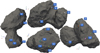 |
Fig. 1 Distribution of 15 selected facets on the surface of 67 P/C-G. Facets 1−11 serve as representative facets for regions exhibiting removal activity in the global dust layer removal simulation, while facets a-d (marked in white) correspond to regions with no removal activity, all of which are located in the northern hemisphere. |
Orbital and rotational parameters of 67P/C-Ga.
3 Modeling comparison and analysis
In this section, we investigate the influence of the porous dust layer properties on sublimation and dust layer evolution. A set of representative surface facets is selected for parameter testing. When analyzing the sensitivity of the simulation results to uncertainties in input parameters, several key factors are considered, including porosity, dust particle size, and initial dust layer thickness. These structural parameters not only directly affect the sublimation process but also determine various physical properties such as tensile strength, permeability, and thermal conductivity (see details in Section 2).
3.1 Selection of representative facets based on illumination
According to the analysis of the dust layer removal model for spherical nucleus by Xin et al. (2024), dust layer activity is almost entirely governed by variations in input solar flux. Based on this finding, the dust layer removal model with parameters listed in Table 2 was applied to simulate the entire surface of comet 67P/C-G in order to identify regions exhibiting dust removal activity. We then performed a clustering analysis of the solar irradiation curves across the surface to group facets with similar illumination behaviors (see Appendix B for details of the clustering method). As a result, 15 representative facets were selected in 15 identified clusters, including 11 active facets exhibiting dust removal activity and 4 inactive facets without removal activity. Note that all surface regions exhibit gas activity; here, “active” and “inactive” refer specifically to dust removal activity.
Table 3 lists the coordinates and associated regions of the representative facets, and their spatial distribution is shown in Figs. 1 and A.2. Notably, the inactive facets are located in the northern hemisphere, which are not illuminated near perihelion.
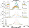 |
Fig. 2 From top to bottom, the panels show (1) the weighted water production rates of the 11 representative facets under the dust layer removal model; (2) the corresponding rates under the constant dust layer model; and (3) the solar illumination curves of each facet. The vertical dashed lines indicate the time of perihelion passage. The insets in each panel provide a magnified view of the near-perihelion region (± 100 days), highlighting differences in peak timing, amplitude, and asymmetry between the two models, as well as their response to the rapidly changing solar flux. |
3.2 Dust layer removal model vs. constant dust layer model
To examine the characteristic dust removal behavior from the dust layer removal model, we focus on the 11 active representative facets identified from Section 3.1 and compare their water production patterns with those obtained from a constant dust layer model. This comparison highlights how dust layer dynamics modulate local activity beyond the response to solar input alone.
The top two panels in Fig. 2 show the weighted water production rate curve of 11 representative facets exhibiting dust removal activity, as computed using the dust layer removal model and the constant dust layer model, respectively. The bottom panel presents the corresponding illumination curves for each representative facet. The water production rate shown for each facet in the figure is defined as Q=A · Qm, where A=Σ Ai denotes the total area of all facets within the corresponding cluster (used as a weight), and Qm is the rotation-averaged water production rate of the representative facet. The structural parameters of the dust layers employed in the models, including porosity, particle size, and initial dust layer thickness, are listed in Table 2. The dust layer structure of the constant dust layer is the same as that of the removal model, and the thickness is always kept at 2 mm.
The comparison between the dust layer removal model and the constant dust layer model (see Fig. 2) reveals that both models exhibit broadly similar trends in the temporal evolution of water production rates. In each case, the overall shape of the production curve closely follows the solar insolation profile. This strong correlation leads to comparable curve morphology and similar peak and peak timings between the two models. This is primarily because, in the dust layer removal model, the average dust layer thickness near perihelion is comparable to the fixed value assumed in the constant dust layer model, resulting in similar sublimation efficiency.
However, at finer temporal scales, clear differences arise due to the distinct mechanisms governing dust evolution in the two models. The constant dust layer model assumes a fixed insulating layer, resulting in a stable thermal conduction regime in which the water production rate responds smoothly to solar insolation without abrupt changes. By contrast, the dust layer removal model exhibits three distinct features. First, it produces a sharp increase in the water production rate shortly before perihelion, reflecting the onset of dust removal activity. Second, during the dust ejection phase, the water production curve displays pronounced oscillations. Third, the termination of cyclical removal activity is marked by a noticeably sharp “elbow” compared to the smooth decrease seen in the constant model.
These behaviors result from the model’s dynamic treatment of the surface dust layer. As the comet approaches perihelion, the continuous accumulation of surface dust results in a more gradual increase in water production rate than that observed in the constant dust layer model. Meanwhile, two coupled effects – intensifying solar insolation and the progressively thickening dust layer – jointly contribute to a continuous temperature increase at the bottom of the dust layer. Specifically, enhanced solar heating provides increased energy input, while the accumulating dust layer acts as an insulating barrier, limiting heat dissipation and causing thermal energy to accumulate beneath it. Consequently, the rising subsurface temperature enhances the sublimation rate of the underlying ice, increasing gas pressure beneath the dust layer. Once this gas pressure surpasses the tensile strength of the dust layer, a dust ejection event is triggered, causing a sudden, sharp rise inflection point in water production.
Following the ejection, dust gradually reaccumulates, gradually inhibiting sublimation until the next ejection condition is reached, thus producing a self-regulating cycle of short-term accumulation and instantaneous removal. This process continues until the decreasing solar flux is no longer sufficient to trigger further ejection, after which sustained dust accumulation results in a relatively sharp “elbow” in the water production curve.
Overall, the resulting water production curve from the dust layer removal model can be understood as a combination of two components: a smooth average baseline resembling the constant dust layer case and a superimposed oscillatory signal linked to dust removal activities. This formulation underscores the relationship between the two models: while the constant dust layer model captures the long-term insolation-driven behavior, the dust layer removal model incorporates additional transient, physically triggered activity.
Furthermore, Fig. 2 illustrates that the cyclical behavior – namely, the frequency, amplitude, and duration – varies across individual facets. These variations appear to depend strongly on both the local input energy and the structural properties of the dust layer. To quantitatively assess how these parameters affect dust layer dynamics, the following sections present a systematic parameter analysis based on the 11 representative facets exhibiting dust layer removal activity, focusing specifically on how each parameter modulates the oscillatory.
3.3 Dust particle size and effective porosity
In our model, porosity directly acts as a multiplier in the equation defining the energy balance at the boundary of the porous layer. Furthermore, porosity and dust particle size jointly influence the mean free path within the dust layer as Eq. (A.3), thereby significantly affecting key physical properties such as permeability, radiative thermal conductivity, and tensile strength (see Eqs. (A.4), (A.5) and (3)). Based on observational estimates (Biele et al. 2022), we adopt surface porosity values close to the measured range, selecting ϕ=0.6, 0.7, and 0.8. Each porosity is tested for two dust particle sizes: ra=1 mm and 0.1 mm. The initial dust layer thickness was set to twice the particle radius (i.e., L0=2 ra) to ensure consistent initial permeability across cases. A summary of the specific model parameters is provided in Table 4, with the corresponding simulation results shown in Fig. 3.
Panels of the left column in Fig. 3 show the water production rate profiles for dust layers composed of 1 mm particles. As porosity increases, the curves exhibit earlier onset times of dust removal, extended durations of cyclical behavior, and higher peak water production rates. At higher porosity, dust removal may activate more facets, including those that remained inactive or ceased activity before perihelion at lower porosities. Moreover, the water production profiles near perihelion appear smoother at higher porosity. This smoothing does not indicate the absence of ejection events but rather results from frequent dust removal activities within each rotation period, producing an averaged, continuous curve.
These trends can be attributed to the microphysical effects of increased porosity. A higher porosity enhances the mean free path, leading to increased permeability. At the same time, higher porosity improves the radiative thermal conductivity, which promotes more efficient heat transfer through the dust layer to the underlying ice. This enhanced heat flux raises the ice temperature, significantly increasing the sublimation rate. The resulting increase in internal gas pressure, combined with the reduced tensile strength, triggers more frequent dust ejection events.
For dust layers composed of smaller particles (0.1 mm), little or no dust removal activity is observed at lower porosities, as shown in the first two panels on the left in Fig. 3. Water production remains low, smooth, and roughly an order of magnitude lower than that of layers with a particle radius of 1 mm. However, with increased porosity, dust ejection is reactivated, leading to pronounced high-amplitude oscillations and a significant enhancement in water production.
These findings highlight the coupled influence of porosity and particle size on the dynamic response of sublimation-driven activity. Higher porosity facilitates both thermal transport and gas escape, promoting active removal behavior, while smaller particles tend to suppress the removal activities by narrowing pore channels, reducing thermal conductivity, and increasing tensile strength. Only under sufficiently porous conditions can fine-grained layers sustain dynamic dust removal and exhibit oscillatory water production signatures. Therefore, to quantitatively capture the combined effects of these two interdependent parameters, a self-consistent numerical simulation framework, such as the dust layer removal model presented in this study, is essential.
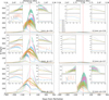 |
Fig. 3 Variation of the water production rate near perihelion under the dust layer removal model for different combinations of dust particle size and porosity. Each panel shows simulation results for a specific particle size (1 mm or 0.1 mm) and three porosity values (0.6, 0.7, and 0.8), as indicated in the bottom-right corner of each subplot. The vertical dashed line marks the time of perihelion passage (x=0). The insets highlight the detailed structure of cyclic dust removal activity near perihelion. In each panel, the upper and lower insets correspond to cases from Fig. 2 that exhibit sustained activity across perihelion and those in which dust removal ceases before perihelion, respectively. |
3.4 Initial dust layer thickness
The initial thickness of the dust layer influences the onset of sublimation-driven dust ejection through its dual role in regulating gas permeability and heat transfer. In this analysis, we fixed the porosity and dust particle radius to the reference values from Fig. 2 (ϕ=0.6, ra=1 mm) and varied the initial dust layer thickness from 2 mm to 0.5 m. The upper bound of 0.5 m was chosen based on the estimated thermal skin depth of cometary nuclei, i.e., the distance that a heat wave can propagate during one rotation period, which is typically less than 0.5 m (Davidsson & Skorov 2002). Fig. 4 illustrates how the onset and termination times, heliocentric distances, and corresponding energy inputs of dust removal events vary over an orbital period as a function of the initial dust layer thickness.
The results indicate that increasing the initial thickness leads to a nonmonotonic shift in the onset position of the first dust ejection, with the heliocentric distance initially increasing and then decreasing, producing a U-shaped trend (see top panels in Fig. 4). This behavior reflects a nonlinear response arising from the interplay between reduced permeability (Π ∝ 1/L) and an increasing thermal conduction path, both of which jointly affect the rate of subsurface gas pressure buildup (see Fig. 5).
Despite these variations in the onset of removal activity, the influence of initial thickness remains modest: the shift in helio-centric distance is limited across the tested range, and even when the thickness varies by two orders of magnitude, the oscillation frequency of ejection changes by at most one cycle, with little variation in interval or amplitude (see Fig. A.3). This behavior is expected, as the “memory” of the initial layer thickness is lost after the first crust shedding. Only a few facets (e.g., facets 1, 8, 9, and 11) exhibit discrete shifts of up to 0.2 AU in their final ejection positions (see lower panels of Fig. 4). These rare shifts can determine whether one additional ejection event is triggered before removal conditions subside (see Fig. 6), resulting in slight variations in the final dust layer thickness (see Fig. 7).
Overall, the system exhibits localized sensitivity due to postreset accumulation dynamics but maintains stable behavior across a broad range of initial conditions. These results highlight the robustness of the dust layer removal model with respect to initial dust thickness and suggest that, once reset to a bare-ice surface, the comet can sustain recurrent activity over successive orbital cycles through a self-regulating accumulation-ejection mechanism.
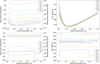 |
Fig. 4 Variations in dust removal activity with respect to initial dust layer thickness. Top row: time and heliocentric distance (left column) and energy flux (right column) of the first removal event. Bottom row: corresponding values for the last removal event. The x-axis in each panel represents the initial dust layer thickness. |
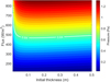 |
Fig. 5 Color map of the variation in subsurface pressure (Pa) as a function of dust layer thickness (m) and input solar flux (W/m2). The color scale indicates the vapor pressure at the boundary beneath the porous layer. The white curve marks the critical pressure of 0.64 Pa, which corresponds to the tensile strength of the dust layer properties. Regions above this threshold suggest conditions under which dust ejection may be triggered. |
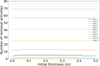 |
Fig. 6 Variation in the number of removal cycles as a function of the initial dust layer thickness. |
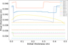 |
Fig. 7 Final dust layer thickness after one orbit as a function of the initial dust layer thicknesses. |
4 Results
4.1 Water production ratio analysis
To evaluate the validity of our dust layer removal model, we compare it with the results from Attree et al. (2023) and Attree et al. (2024). These studies employed a parameterized activity model of 67P/C-G, which was optimized to reproduce key observational constraints, namely the evolution of the comet’s rotational state, orbital motion (including non-gravitational effects), and water production rates. While their approach infers the effective activity distribution by fitting global dynamical and production data, our model is designed to investigate the underlying microphysical processes of dust-layer removal.
Attree et al. (2023) divided the surface of 67 P/C−G into six super-regions, each assigned an effective active fraction (EAF). For the two southern super-regions, the EAF was allowed to vary with time, while the others remained constant. The activity in these southern regions displayed a clear asymmetry, characterized by a rapid increase near perihelion followed by a pronounced post-perihelion tail. In contrast, activity in the northern regions remained persistently weak throughout the orbit. In Attree et al. (2024), the surface was divided according to geomorphological features described by Thomas et al. (2018), separating the northern and southern hemispheres into “dusty” and “rocky” regions, with illumination changes incorporated more explicitly.
We calculate the ratio of water production rates for each of the three dust layer models – constant dust layer, growing dust layer, and dust layer removal – relative to Model A, expressed as QB/QA, which is equivalent to the EAF. These models are discussed in Xin et al. (2024). This comparison is performed for the 15 selected representative facets introduced in Section 3.1, including both facets with and without dust removal activity. We adopt a fixed thickness of 0.002 m for the constant dust layer model and an initial thickness of 0.002 m for both the dust layer growing and removal models. The dust layer structure follows the parameters listed in Table 2. During periods without solar insolation, QB/QA is set to 0 to indicate the absence of sublimation activity. The results for the three models are shown from top to bottom in Fig. 8.
By comparing the QB/QA curves from these three models, we aim to demonstrate that only the dust layer removal model among the three can reproduce the consistent inhomogeneous time evolution characteristics in Attree et al. (2023) and Attree et al. (2024). The constant dust model, which assumes a permanently insulating surface layer, produces a smooth production ratio curve that purely follows solar flux and lacks any pronounced peak near perihelion. Moreover, it fails to distinguish between regional differences in response to solar insolation, resulting in uniformly scaled activity across the surface. The growing dust layer model captures the continuous process of dust accumulation, which leads to an early peak in activity. However, as the layer thickens, sublimation becomes increasingly suppressed, preventing the emergence of a significant activity peak near perihelion. Although the rate of suppression varies with solar insolation, this model lacks a mechanism to generate sharply differentiated regional activity and thus fails to reproduce the distinct EAF curves in different regions shown in Attree et al. (2023) and Attree et al. (2024).
In contrast, the dust layer removal model incorporates a physically motivated mechanism of pressure-driven ejection. This process naturally produces sharp inflection points and oscillatory peaks in QB/QA near perihelion for southern hemisphere facets, closely resembling the time-varying EAF enhancements observed in Attree’s southern super-regions. The model effectively captures both the intense activity near perihelion and the marked asymmetry between pre- and post-perihelion phases.
Furthermore, the model successfully reproduces the contrasting behavior between hemispheres. Facets located in strongly irradiated regions near perihelion – corresponding to the comet’s local summer – undergo repeated dust ejection cycles, leading to episodic enhancements in sublimation. Conversely, facets in weakly illuminated northern regions accumulate dust without removal, leading to persistent activity suppression. This self-regulating response to local solar flux conditions gives rise to a spatiotemporal pattern of activity that closely mirrors the temporal and spatial asymmetry observed in Attree et al. (2023) and Attree et al. (2024).
Note that in Attree et al. (2023) and Attree et al. (2024), the EAF curves were derived through finding the best mathematical optimization, not by physical modeling. Our dust layer removal model offers a self-consistent, physically grounded explanation for these behaviors, demonstrating for the first time that such spatiotemporally asymmetric activity patterns can emerge from thermophysical processes on the cometary surface.
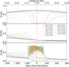 |
Fig. 8 Ratio of gas production rates of different models and Model A for representative facets (among them, facets 1-11, which are active, have removal activity in the global simulation, while facets a-d, which are inactive, in a gray color have no removal activity in the global simulation). From top to bottom, they represent the constant dust layer model (with a fixed thickness of 0.002 m), the growing dust layer model, and the dust layer removal model, which were all initialized with a dust layer thickness of 0.002 m. |
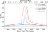 |
Fig. 9 Comparison between the simulated results of the dust layer removal model and the EAF curves from Attree et al. (2023). The solid and dashed gray lines are directly taken from Fig. 2 of Attree et al. (2023), representing the EAF evolution in southern and other regions, respectively. Solid red and blue lines indicate the total water production from active facets in the dust removal model (porosity ϕ=0.78 and 0.74, respectively), normalized by Model A. Dashed lines show the corresponding ratios for inactive facets. In all cases, the dust particle radius was set to 0.1 mm, and the initial dust layer thickness was set to 4 cm. |
4.2 Analysis based on EAF
Fig. 9 presents a comparison between the simulated water production rate ratio from the dust layer removal model and the EAF curves derived by Attree et al. (2023). In the figure, the gray solid lines represent the active fraction for the two southern super-regions defined by Attree et al. (2023), with the higher peak corresponding to the region with positive torque efficiency and the lower peak corresponding to the region with negative torque efficiency. The gray dashed lines denote the remaining regions in Attree et al. (2023) with lower constant activity, including the equatorial areas, the base of the comet body, the top of the head, and the individual Hathor and Hapi regions.
The dust layer removal simulations were conducted using a dust particle radius of 0.1 mm and an initial dust layer thickness of 4 cm. This relatively thick initial layer was chosen to suppress early sublimation and better match the low activity observed at large heliocentric distances. To qualitatively match the EAF curves of the southern regions, simulations of the 15 representative facets were conducted across a range of porosity values. For each porosity value, we computed the total water production rate Σ QB over either the active or inactive facet group and normalized it by the corresponding Model A total production Σ QA to obtain the ratio Σ QB/Σ QA.
To improve the clarity of the resulting curves and facilitate comparison with observed trends, a two-step filtering procedure was applied. First, a median filter was used to remove local spikes in the peak region. Then, Savitzky-Golay filtering was used to smooth the curve profiles while preserving their overall trends.
Among the tested cases, we identified two key bounds: the minimum porosity required to trigger dust removal activity and the maximum porosity that keeps the peak value of the ratio Σ QB/Σ QA below approximately 0.45. As illustrated in Fig. 9, only the results at these two limits are shown for clarity. The solid red and blue lines correspond to the summed water production ratios of active facets for the upper and lower porosity limits, respectively. The dashed lines show the corresponding results for inactive facets. Increasing porosity leads to higher peak values as well as a broader temporal extent of the ratio response.
The results show that within the porosity range of 0.74−0.78, the dust layer removal model qualitatively reproduces the amplitude, asymmetry, and duration of the southern EAFs, although the peak occurs about 30 days earlier than in the EAF curves. This offset arises from the fundamental differences in the underlying sublimation models. While Attree et al. (2023) employed empirical EAF scaling factors to adjust Model A, the dust layer removal model directly couples sublimation, pressure build-up, and dust removal processes.
The feasible porosity-size parameter space is further constrained by simulations over particle radius ranging from 0.1 mm to 1 mm (see Fig. 10). The shaded region in the figure indicates the feasible domain for porosity values, with an uncertainty of approximately 0.01. Both the lower and upper porosity limits decrease with increasing particle size, reflecting the influence of particle size on permeability.
Within this constrained parameter space, we compared the model output with the latest EAF optimization from Attree et al. (2024), who incorporated differences in transfer efficiency between rocky and dusty terrains and accounted for seasonal illumination changes. The light-colored curves in Fig. 11 (taken from Fig. 5 in Attree et al. 2024) show the optimized EAF evolution in four super-regions: southern and northern rocky and dusty areas. The dark curves are our model results obtained by grouping representative facets accordingly (see Fig. A.4) and calculating their total normalized production ratios. For rocky facets we assumed an initial thickness of 4 cm, while dusty facets were assigned 6 cm. Using a particle radius of 0.1 mm and a porosity of 0.74 (i.e., the lower limits in Fig. 10), the model qualitatively reproduces the sharp peaks of the southern regions at perihelion. The rocky region shows higher peak activity than the dusty region, consistent with its more frequent dust removal times and seasonal insolation, which may also explain dust accumulation in the latter. However, pre-perihelion is underestimated, likely because the model only considers water ice sublimation. Actually, CO2 sublimation could also drive dust lifting and expose new active patches around 200 days before perihelion (Filacchione et al. 2016). For the northern hemisphere, both rocky and dusty regions show no dust activity, consistent with the growing dust layer model; their trends are controlled more by solar illumination than by dust evolution, owing to weaker insolation and a slower buildup of the dust layer.
Finally, to illustrate the spatial heterogeneity, we compared the dust layer removal model with the global EAF distribution reconstructed by Kramer et al. (2019) from the change in rotation period and the orientation of the rotation axis of 67P/C-G. Using the dust layer removal model, we computed the total water production ratio (QB/QA) for each facet integrated over ± 300 days around perihelion. Fig. 12 shows the total water production ratio, normalized by its global mean value. The right panel presents the zonally averaged values as a function of latitude, with the blue shaded band indicating the 1−σ variability within each latitude bin. The model produces the overall trend of higher southern and lower northern activity than the averaged production ratio, in broad agreement with Kramer et al. (2019). However, differences remain due to methodology: the analysis in Kramer et al. (2019) relied on 36 large surface patches, while our facet−based model captures finer−scale heterogeneity. Especially in the equatorial belt (−30° to +30°), our results show substantial variability, indicating that simple zonal averages may not reliably represent local conditions.
Taken together, these comparisons demonstrate that the dust layer removal model can reproduce both the temporal evolution of cometary activity and the spatial heterogeneity, providing a physically consistent framework for explaining the cometary activity evolution. While idealized assumptions – such as fixed porosity and monodisperse particle size – were adopted, they help isolate fundamental mechanisms. Incorporating factors such as polydispersity may refine the results but is not expected to alter qualitative behavior.
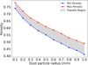 |
Fig. 10 Feasible porosity range as a function of dust particle sizes. The blue and red curves represent the minimum and maximum porosity values required for reproducing the modeled activity as in Fig. 9. The shaded area between them denotes the feasible parameter space in which the dust layer removal model produces plausible results consistent with the EAF curves. |
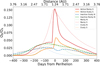 |
Fig. 11 Comparison between the simulated results of the dust layer removal model and the EAF curves from Attree et al. (2024). The light-colored curves are taken from Fig. 5 of Attree et al. (2024), showing the EAF evolution in the four representative regions. Dark curves represent the normalized water production from the dust layer removal model, with colors matching the corresponding representative facets shown in Fig. A.4. |
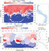 |
Fig. 12 Comparison between the dust layer removal model results and the surface active fraction map in Kramer et al. (2019). Top panel: spatial distribution (left) and latitudinal profile (right) of the water production ratio between the dust layer removal model (QB) and the reference Model A (QB), normalized by its global mean and integrated over ± 300 days around perihelion. The shaded blue area indicates the 1−σ variability within each latitude band. Bottom panel: surface active fraction relative to the average value (left) and its zonal mean profile (right), reproduced from Fig. 10 of Kramer et al. (2019). |
5 Discussion
The primary objective of this study is to present a physically consistent microphysical model of an evolving cometary surface layer, accounting for orbital motion, nucleus rotation, complex shape, and local illumination. Microphysical parameters used in the thermal modeling are derived from numerical simulations and analyses of laboratory experiments. Comparison with local gas production curves demonstrates that the model captures observed activity patterns, although certain simplifications and unmodeled physical effects may affect detailed accuracy.
Most modern thermal models assume a homogeneous nucleus with fixed porosities, particle size, and nonvolatile-to-volatile mass ratio. The simplified assumption, uniform dust layer structure, has been effectively applied to a range of cometary problems, for example, in reproducing certain instantaneous observational features (Kramer & Noack 2016) and in studying the evolving activity features (Marshall et al. 2019; Xin et al. 2024). Nevertheless, such simplified treatments cannot fully represent the microphysical heterogeneity of cometary surfaces. Incorporating additional complexity – such as polydisperse particle sizes, stratified structures, or spatially varying dust-to-ice ratios – may improve model realism, but at the cost of introducing poorly constrained parameters. A stepwise refinement strategy is therefore advisable, beginning with idealized geometries such as spherical nuclei, and then systematically assessing the impact of added physical complexity.
In addition to the microphysical simplifications, the current model considers only water ice sublimation and neglects the potential role of supervolatiles such as CO2. Observations suggest that CO2 outgassing significantly contributes to activity in many regions of the nucleus, for instance, by triggering the ejection of water-ice-rich fragments, contributing to nongravitational accelerations (NGAs), or producing bright surface spots at large heliocentric distances (Attree et al. 2023; Gundlach et al. 2015). Ignoring these processes may limit the ability of the model to capture early activity patterns, compositional variations, and the detailed origin of nongravitational forces (NGFs). In our simulations, the first major dust removal event occurs approximately 100 days before perihelion, with the surface darkening and accumulating dust prior to that point. By contrast, bright spots have been observed as early as ∼ 300 days before perihelion, suggesting additional mechanisms may be at play. These features may arise from early CO2 activity or localized structural weaknesses that enable premature crust disruption.
Another point is gas heating during diffusion through the dust layer, which alters the velocity distribution of escaping gas molecules and thus modifies the momentum flux and reactive forces. Studies have shown that the thermal velocity of gas at the surface can approach nearly twice that at the sublimation front (Skorov et al. 2024a). This effect, together with internal conductive fluxes, modifies the thermodynamics at the sublimation front. Therefore, the inclusion of these thermal processes in gas dynamics is essential when moving from qualitative analyses to quantitative modeling of NGAs.
Overall, the above simplifications and neglected physical processes may directly affect the model’s ability to represent nongravitational effects. To evaluate this impact, we calculated the three components of the NGA using the dust layer removal model (see Fig. A.1 and Appendix C) and compared them with the results of Kramer & Läuter (2019) and Manghi et al. (2025), who reconstructed the accelerations from the spacecraft trajectory. Our model reproduces the observed seasonal trends qualitatively, but it systematically yields sharper perihelion peaks and a more rapid post-perihelion decay. In particular, the z -component decreases rapidly after perihelion, regardless of adjustments to dust-layer structural parameters. This systematic deviation reflects the intrinsic tendency of the dust-removal scheme toward producing a strong perihelion maximum. The omission of CO2 sublimation is likely a key factor, as CO2 activity may contribute substantially to sustaining accelerations beyond perihelion. Besides, factors such as a nonuniform dust mantle, heterogeneous distributions of water ice, and transient thermophysical properties are also expected to influence both the amplitude and temporal evolution of the NGA curves and should be considered in future refinements of the model.
In addition to the microscopic unmodeled processes, several macroscopic simplifications may influence the accuracy of the simulations. These include radiative effects related to surface roughness, such as shading and self-heating, which can significantly impact the local energy balance, gas flow, and the resulting NGFs. Shading suppresses sublimation by reducing incident solar flux, while self-heating from neighboring facets may enhance energy absorption in concave areas (Rezac & Zhao 2020; Zhao et al. 2020; Hu et al. 2017a). These effects can shift the timing and intensity of sublimation-driven dust layer removal activity and are especially important for capturing small-scale heterogeneity.
Gravitational stress serves as a supplementary resisting force against gas-driven dust ejection. According to Bischoff et al. (2023), under a constant surface gravity of 2 × 10⁻⁴ m/s2, the gravitational stress for centimeter-scale particles becomes significant only when the dust layer thickness exceeds several decimeters. For layers thinner than 1 dm, the gravitational stress typically remains below 0.01 Pa, substantially lower than the tensile strength thresholds assumed in this study. However, in extreme scenarios where the dust layer becomes highly porous and cohesive strength drops considerably, gravity may act as the final resisting force against dust ejection. Evaluating such gravitational constraints in potentially loose or weakly bound surface regions remains an important direction for future work.
Most notably, the fallback of ejected dust represents a potentially significant feedback mechanism. According to Lai et al. (2017), fallback flux in regions such as Hapi can reach up to 20 kg/m2 / month near perihelion, corresponding to a maximum redeposition thickness of ∼ 0.6 mm per rotation, assuming a bulk density of 530 kg/m3. Under similar conditions, our model predicts an in situ dust accumulation rate of ∼ 0.4 mm due to ice sublimation per rotation, suggesting that fallback and sublimation-driven accumulation may be comparable in magnitude in favorable regions. However, such extreme fluxes are likely confined to a limited number of concave or low-gravity regions, while most regions experience substantially lower redeposition. Consequently, although fallback could influence the local evolution of the dust layer and the triggering threshold for ejection, its omission is considered justified at the global scale. Within the spatial resolution and physical assumptions of our model, neglecting fallback does not significantly affect the robustness or physical plausibility of the results.
6 Conclusions
In this study, we develop and analyze a new dust layer removal model within the MONET framework to systematically simulate the coupled dynamical evolution of the porous dust layer and the corresponding sublimation processes on 67P/Churyumov-Gerasimenko. The core idea of the model is the dynamic switching between a pure ice sublimation model (Model A) and a homogeneous dusty layer model (Model B), allowing us to describe the processes of dust accumulation and pressure-driven dust removal activities and to investigate their modulation of water production rates and nongravitational forces.
Research has shown that the onset of a cyclic regime is a highly stable process, largely independent of crust thickness at aphelion. This finding confirms the existence of a general cyclic behavior in the surface region, rather than a special solution tied to specific parameter choices. Consequently, it, for the first time, demonstrated the feasibility of modeling long-period activity when abandoning the nonphysical assumption of a constant thickness of the porous dry crust covering the icy region. The initial dust layer thickness induces only a slight temporal shift in the beginning of dust removal activity, without significantly affecting the overall dynamical behavior.
By computing the thermophysical evolution from the model surface shape over 67P/C-G’s orbit, we captured the repeating cycles of dust accumulation and ejection triggered by subsurface gas pressure under different dust layer structures. The results show that the model is sensitive to microscopic parameters of the dust layer. Specifically, porosity and dust grain size strongly influence permeability, thermal conductivity, and tensile strength, which in turn determine the time of first removal activity, the frequency of removal activities, and the peak sublimation rate.
We introduced a clustering method based on solar insolation profiles to identify representative surface facets for parameter analysis and qualitatively compare the model results with fitting EAF curves and distributions reported in the literature. The results show that, within a realistic range of dust layer parameters, the dust layer removal model qualitatively reproduces the basic characteristics of the southern hemisphere EAF curves. More importantly, the model self-consistently selects active and inactive regions in response to local incident solar flux, resulting in a spatially heterogeneous distribution of gas and dust activities.
Therefore, the dust layer removal model matches the fitting results of nongravitational effects in terms of both the temporal evolution and the spatial active distribution. This provides a reasonable physical scenario for revealing the non-steady-state sublimation mechanism on the comet surface, which explains the formation of local high-activity and low-activity areas and allows for us to understand the nongravitational disturbances.
In conclusion, despite the ability of the model to reproduce key aspects of cometary activity, further refinements are essential to enhance its physical realism. Key extensions include the incorporation of non-uniform dust layers, supervolatiles, shading, self-heating, gravity, gas heating, and fallback dynamics. These improvements are particularly important for applications involving inverse modeling of nongravitational forces and the long-term morphological evolution of cometary nuclei.
Acknowledgements
We thank the referee and the editor for their constructive comments and suggestions. YX and YZ were supported by the National Natural Science Foundation of China (Grant Nos. 12222307, 12073084). Yu.S. acknowledges support from ESA through contract 4000141229/23/ES/CM and the Deutsche Forschungsgemeinschaft (DFG) for support under grant BL 298/32-1.
References
- Asaeda, M., Yoneda, S., & Toei, R., 1974, J. Chem. Eng. Jpn., 7, 93 [CrossRef] [Google Scholar]
- Attree, N., Jorda, L., Groussin, O., et al. 2023, A&A, 670, A170 [NASA ADS] [CrossRef] [EDP Sciences] [Google Scholar]
- Attree, Gutiérrez, P., Groussin, O.,, et al. 2024, A&A, 690, A82 [NASA ADS] [CrossRef] [EDP Sciences] [Google Scholar]
- Biele, J., Vincent, J.-B., & Knollenberg, J., 2022, Universe, 8, 487 [NASA ADS] [CrossRef] [Google Scholar]
- Bischoff, D., Schuckart, C., Attree, N., Gundlach, B., & Blum, J., 2023, MNRAS, 523, 5171 [NASA ADS] [CrossRef] [Google Scholar]
- Blum, J., Gundlach, B., Krause, M., et al. 2017, MNRAS, 469, S755 [Google Scholar]
- Davidsson, B. J. R., & Skorov, Y. V., 2002, Icarus, 159, 239 [CrossRef] [Google Scholar]
- El-Maarry, M. R., Thomas, N., Giacomini, L., et al. 2015, A&A, 583, A26 [NASA ADS] [CrossRef] [EDP Sciences] [Google Scholar]
- El-Maarry, M. R., Thomas, N., Gracia-Berná, A., et al. 2016, A&A, 593, A110 [NASA ADS] [CrossRef] [EDP Sciences] [Google Scholar]
- Fanale, F. P., & Salvail, J. R., 1984, Icarus, 60, 476 [NASA ADS] [CrossRef] [Google Scholar]
- Filacchione, G., Raponi, A., Capaccioni, F., et al. 2016, Science, 354, 1563 [Google Scholar]
- Gundlach, B., & Blum, J., 2012, Icarus, 219, 618 [CrossRef] [Google Scholar]
- Gundlach, B., Blum, J., Keller, H. U., & Skorov, Y. V., 2015, A&A, 583, A12 [NASA ADS] [CrossRef] [EDP Sciences] [Google Scholar]
- Güttler, C., Rose, M., Sierks, H., et al. 2023, MNRAS, 524, 6114 [CrossRef] [Google Scholar]
- Hansen, K. C., Altwegg, K., Berthelier, J.-J., et al. 2016, MNRAS, 462, S491 [Google Scholar]
- Hässig, M., Altwegg, K., Balsiger, H., et al. 2015, Science, 347 [Google Scholar]
- Hu, X., Shi, X., Sierks, H., et al. 2017a, MNRAS, 469, S295 [NASA ADS] [CrossRef] [Google Scholar]
- Hu, X., Shi, X., Sierks, H., et al. 2017b, A&A, 604, A114 [NASA ADS] [CrossRef] [EDP Sciences] [Google Scholar]
- Keller, H. U., Delamere, W. A., Huebner, W. F., et al. 1987, A&A, 187, 807 [Google Scholar]
- Keller, H. U., Mottola, S., Davidsson, B., et al. 2015a, A&A, 583, A34 [NASA ADS] [CrossRef] [EDP Sciences] [Google Scholar]
- Keller, H. U., Mottola, S., Skorov, Y., & Jorda, L. 2015b, A&A, 579, L 5 [Google Scholar]
- Kramer, T. & Läuter, M., 2019, A&A, 630, A4 [NASA ADS] [CrossRef] [EDP Sciences] [Google Scholar]
- Kramer, T., & Noack, M., 2016, Astrophys. J. Lett., 823, L 11 [Google Scholar]
- Kramer, T., Läuter, M., Hviid, S., et al. 2019, A&A, 630, A3 [NASA ADS] [CrossRef] [EDP Sciences] [Google Scholar]
- Lai, I.-L., Ip, W.-H., Su, C.-C.,, et al. 2017, MNRAS, 462, S533 [Google Scholar]
- Langevin, Y., Hilchenbach, M., Ligier, N., et al. 2016, Icarus, 271, 76 [CrossRef] [Google Scholar]
- Liu, C., Zhao, Y., & Ji, J., 2023, Acta Astron. Sinica, 64, 11 [Google Scholar]
- Macher, W., Skorov, Y., Kargl, G., Laddha, S., & Zivithal, S., 2024, J. Eng. Math., 144, 2 [NASA ADS] [CrossRef] [Google Scholar]
- Manghi, R. L., Zannoni, M., Tortora, P., et al. 2025, Ephemeris Reconstruction for Comet 67P/Churyumov-Gerasimenko During Rosetta Proximity Phase from Radiometric Data Analysis [Google Scholar]
- Marshall, D., Rezac, L., Hartogh, P., Zhao, Y., & Attree, N., 2019, A&A, 623, A120 [NASA ADS] [CrossRef] [EDP Sciences] [Google Scholar]
- Merouane, S., Zaprudin, B., Stenzel, O., et al. 2016, A&A, 596, A87 [NASA ADS] [CrossRef] [EDP Sciences] [Google Scholar]
- Moehlmann, D., 1994, Planet. Space Sci., 42, 933 [Google Scholar]
- Preusker, F., Scholten, F., Matz, K.-D., et al. 2017, A&A, 607, L1 [NASA ADS] [CrossRef] [EDP Sciences] [Google Scholar]
- Rezac, L., & Zhao, Y., 2020, A&A, 642, A167 [NASA ADS] [CrossRef] [EDP Sciences] [Google Scholar]
- Rotundi, Sierks, H., Della Corte, V.,, et al. 2015, Science, 347 [Google Scholar]
- Skorov, Y., & Blum, J., 2012, Icarus, 221, 1 [Google Scholar]
- Skorov, Y., van Lieshout, R., Blum, J., & Keller, H. U., 2011, Icarus, 212, 867 [NASA ADS] [CrossRef] [Google Scholar]
- Skorov, Y., Rezac, L., Hartogh, P., & Keller, H. U., 2017, A&A, 600, A142 [NASA ADS] [CrossRef] [EDP Sciences] [Google Scholar]
- Skorov, Y., Keller, H. U., Mottola, S., & Hartogh, P., 2020, MNRAS, 494, 3310 [NASA ADS] [CrossRef] [Google Scholar]
- Skorov, Y., Reshetnyk, V., Bentley, M., et al. 2021, MNRAS, 501, 2635 [CrossRef] [Google Scholar]
- Skorov, Y., Markkanen, J., Reshetnyk, V., et al. 2023, MNRAS, 522, 4781 [NASA ADS] [CrossRef] [Google Scholar]
- Skorov, Y., Reshetnyk, V., Markkanen, J., et al. 2024a, MNRAS, 527, 12268 [Google Scholar]
- Skorov, Y. V., Mokhtari, O., Macher, W., et al. 2024b, A&A, 689, A131 [NASA ADS] [CrossRef] [EDP Sciences] [Google Scholar]
- Thomas, N., El Maarry, M. R., Theologou, P., et al. 2018, Planet. Space Sci., 164, 19 [NASA ADS] [CrossRef] [Google Scholar]
- Wächter, A., & Biegler, L., 2006, Math. Program., 106, 25 [CrossRef] [Google Scholar]
- Xin, Y., Skorov, Y., Zhao, Y., et al. 2024, A&A, 693 [Google Scholar]
- Zhao, Y., Rezac, L., Skorov, Y., & Li, J. Y., 2020, MNRAS, 492, 5152 [Google Scholar]
- Zhao, Y., Rezac, L., Skorov, Y., et al. 2021, Nat. Astron., 5, 139 [Google Scholar]
Appendix A Sublimation model
The energy input at the comet nucleus surface originates exclusively from solar radiation. This incoming solar flux determines the absorbed energy balance, which governs the local thermal and sublimation processes. In the case of Model A, we assume the nucleus surface is composed of a uniform, intimately mixed layer of ice and dust, with thermal conduction neglected. The energy balance can be expressed as:
 (A.1)
where S0 is the solar flux at 1 AU(1367 W/m2), Av is the Bond albedo (0.04), and rh is the heliocentric distance. The term ni · s accounts for the projection of the facet normal vector ni onto the direction of the Sun s, ensuring proper spatial dependence of irradiation. On the right-hand side, σ is the Stefan-Boltzmann constant, ε is the emissivity (0.97), and T is the surface ice temperature. The term Z(T) H represents the energy loss due to sublimation. H is the latent sublimation heat, and Z(T) is the sublimation rate determined by the Hertz-Knudsen formula:
(A.1)
where S0 is the solar flux at 1 AU(1367 W/m2), Av is the Bond albedo (0.04), and rh is the heliocentric distance. The term ni · s accounts for the projection of the facet normal vector ni onto the direction of the Sun s, ensuring proper spatial dependence of irradiation. On the right-hand side, σ is the Stefan-Boltzmann constant, ε is the emissivity (0.97), and T is the surface ice temperature. The term Z(T) H represents the energy loss due to sublimation. H is the latent sublimation heat, and Z(T) is the sublimation rate determined by the Hertz-Knudsen formula:
 (A.2)
where P(T) is the saturation vapor pressure, and vth is the thermal velocity of vapor molecules. The latent sublimation heat and the saturation pressure values are obtained from Fanale & Salvail (1984).
(A.2)
where P(T) is the saturation vapor pressure, and vth is the thermal velocity of vapor molecules. The latent sublimation heat and the saturation pressure values are obtained from Fanale & Salvail (1984).
Model B differs from Model A in the introduction of a porous dust layer. The dust layer plays a crucial role in regulating the heat flux to the sublimation front while in parallel limiting the diffusion of water vapor, thereby controlling the water-ice sublimation rate. Consequently, in the two-layer thermophysical model with a porous surface layer, the gas production rate is determined by both the energy transferred to the sublimation front and the gas kinetic resistance of the boundary layer caused by gas permeability (Hu et al. 2017a; Skorov et al. 2017, 2021). The microscopic thermophysical model used in this study includes two key components: generation of a random porous layer and estimation of its transport properties (e.g., permeability and effective conductivity).
Following the approach of Xin et al. (2024), we simulate the Knudsen gas flow through a porous dust layer, built by aggregates, using the Test Particle Monte Carlo (TPMC) method (Skorov et al. 2011). For the purposes of our work, a layer can be completely described by effective porosity (ϕ), aggregate particle size (ra), and dust layer thickness. The effective porosity and aggregate size determine the average pore size or, equivalently, mean free path ( ), which in turn influences two key derived parameters: the permeability of the layer to gas flow and the radiative thermal conductivity.
In the uniform porous medium case, MFP can be expressed as follows (Macher et al. 2024; Güttler et al. 2023):
 (A.3)
where ϕ is the porosity and ra is the radius of aggregates. Following Macher et al. (2024), the permeability Π of a layer of thickness L is expressed as:
(A.3)
where ϕ is the porosity and ra is the radius of aggregates. Following Macher et al. (2024), the permeability Π of a layer of thickness L is expressed as:
 (A.4)
with Lh being the half-transmission length derived from Knudsen reflection law and Maxwellian flux theory (Macher et al. 2024; Asaeda et al. 1974).
(A.4)
with Lh being the half-transmission length derived from Knudsen reflection law and Maxwellian flux theory (Macher et al. 2024; Asaeda et al. 1974).
In a porous dust layer, heat transfer is governed by gas convection, solid contact conduction, and radiative heat conductivity through pores, i.e., Keff(T)=Ksolid(T)+Krad(T)+Kgas (Gundlach & Blum 2012; Skorov et al. 2021). Due to the low-pressure environment of the cometary surface, the effect of gas convection is negligible (Fanale & Salvail 1984). The calculation of solid thermal conductivity is based on the Hertz theory (see Gundlach & Blum (2012) for details). Radiative thermal conductivity depends on the cube of temperature and the average pore size  :
:
 (A.5)
(A.5)
Incorporating a temperature-dependent effective heat conductivity and the resistance of the dust layer to gas flow, we establish a 1D two-layer dust model to describe energy conservation. The upper and lower boundaries of the dust layer can be expressed as
 (A.6)
(A.6)
 (A.7)
where Π is the permeability of the layer, Keff(T) and
(A.7)
where Π is the permeability of the layer, Keff(T) and  are the effective heat conductivities of the porous dust layer and the icy medium, respectively. The difference between the thermal conductivity of dust and ice is considered negligible in this analysis due to their small values and minimal effect on the heat flux to the interior (Skorov et al. 2024b; Xin et al. 2024).
Appendix B Selection of representative facets
To capture the geometrically induced diversity in solar irradiation on comet 67 P/C-G, we performed a clustering analysis based on the temporal evolution of heliocentric solar flux.
Specifically, we first analyzed precomputed energy flux profiles (solar input) for all facets. Only data within 3 AU of the Sun were retained to focus on the active orbital segment. To extract relevant features for clustering, we applied a discrete wavelet transform (DWT) to each flux curve. This transformation captures both global trends and localized fluctuations, thereby encoding multiscale temporal features.
Next, we applied z-score normalization to the feature vectors, followed by principal component analysis (PCA) to reduce dimensionality and denoise the data. We then performed K-means clustering with 15 random restarts to ensure solution stability. The optimal number of clusters was determined using the elbow method based on within-cluster sum of squares (WCSS). We plotted the WCSS as a function of the number of clusters. As the cluster number increases, WCSS decreases, but the rate of decrease gradually slows down. The point at which the curve begins to flatten – commonly referred to as the “elbow” – is considered to indicate the optimal number of clusters.
For each cluster, we computed a pointwise median curve by collecting all member curves on a common temporal grid and taking the median flux at each time step. The most representative curve in each cluster was then identified as the one with the smallest Euclidean distance to the median curve. The corresponding facet was marked as the cluster representative facet and highlighted in Fig. A.1 with red color.
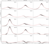 |
Fig. A.1 Cluster analysis of solar illumination curves for facets with and without dust layer removal activity, based on global simulations using the dust layer removal model. The red curves indicate the selected representative facets within each cluster. Facets 1-11 correspond to active regions exhibiting dust removal activities, while facets a-d represent inactive regions with no dust removal activity. |
This clustering analysis was performed independently for active and inactive facets to account for the distinct variability patterns between them. The identified representative facets were used as proxies for their respective groups in simulations and discussions.
Appendix C Nongravitational acceleration analysis
Fig. A.1 compares the NGAs of comet 67P/C-G obtained from the dust layer removal model with observationally reconstructed results from Kramer & Läuter (2019). The modeled NGA curves exhibit qualitative consistency with the observations: the y – and z -components peak shortly after perihelion and decay rapidly with heliocentric distance, while the x -component reaches a positive maximum prior to perihelion and then reverses its sign. This overall seasonal pattern reflects the combined influence of orbital geometry, spin-axis orientation, and illumination conditions, rather than the dust-removal mechanism alone.
Under the dust layer composed of 0.6 mm particles and a porosity of 0.6 (upper limit in Fig. 10), the NGA components start to rise about 80 days before perihelion, consistent with reconstructed curves. At lower porosities, the increased tensile strength and reduced permeability suppress activity, delaying its onset and producing fewer active facets, as Section 3.3 illustrates. In such cases, the modeled NGA curves are comparable to the overall magnitude of the observed accelerations, although their temporal profiles are not closely aligned.
Besides the general agreement, the model does not fully reproduce the observed NGA. Several factors may contribute to the discrepancies: (i) the assumption of a homogeneous dust layer with fixed particle size and porosity, (ii) unresolved local surface morphology, (iii) heterogeneous water-ice distribution, (iv) use of a simplified two-layer thermophysical model, and (v) the potential dominance of CO2 sublimation near perihelion, implying a different sublimation front. The mismatch is particularly pronounced for the z-component, which in observations decays more slowly after perihelion than in the model. This bias reflects the tendency of the dust-removal framework to emphasize perihelion maxima.
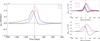 |
Fig. A.1 Comparison of modeled and observed NGA curves of 67P/C-G. Left panel: NGA of 67P/C-G in the terrestrial equatorial frame, evaluated under the dust layer removal model composed of 0.6 mm particles and a porosity of 0.6. Right panel: Fig. 2 from Kramer & Läuter (2019), showing the observed NGA (top) and the Marsden model simulation (bottom). Both panels are plotted on the same vertical scale for direct comparison. |
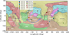 |
Fig. A.2 Locations of selected facets, identified through clustering analysis of illumination curves, are marked on the 67P/C-G comet 2D map from El-Maarry et al. (2016). In this representation, facets labeled “R” indicate regions where removal activity occurs in the global simulation of the dust layer removal model for 67P/C-G, whereas those labeled “NR” correspond to regions where no removal activity is observed in the simulation. |
 |
Fig. A.3 Simulated water production rates for the 11 selected surface facets under two different initial dust layer thicknesses: 2 mm (left) and 200 mm (right). |
 |
Fig. A.4 Locations of selected representative facets, labeled with colors matching the four super regions in Fig. 5 of Attree et al. (2024). These facets were grouped according to the regional classification to derive the model curves shown in Fig. 11. |
All Tables
All Figures
|
Fig. 1 Distribution of 15 selected facets on the surface of 67 P/C-G. Facets 1−11 serve as representative facets for regions exhibiting removal activity in the global dust layer removal simulation, while facets a-d (marked in white) correspond to regions with no removal activity, all of which are located in the northern hemisphere. |
| In the text | |
|
Fig. 2 From top to bottom, the panels show (1) the weighted water production rates of the 11 representative facets under the dust layer removal model; (2) the corresponding rates under the constant dust layer model; and (3) the solar illumination curves of each facet. The vertical dashed lines indicate the time of perihelion passage. The insets in each panel provide a magnified view of the near-perihelion region (± 100 days), highlighting differences in peak timing, amplitude, and asymmetry between the two models, as well as their response to the rapidly changing solar flux. |
| In the text | |
|
Fig. 3 Variation of the water production rate near perihelion under the dust layer removal model for different combinations of dust particle size and porosity. Each panel shows simulation results for a specific particle size (1 mm or 0.1 mm) and three porosity values (0.6, 0.7, and 0.8), as indicated in the bottom-right corner of each subplot. The vertical dashed line marks the time of perihelion passage (x=0). The insets highlight the detailed structure of cyclic dust removal activity near perihelion. In each panel, the upper and lower insets correspond to cases from Fig. 2 that exhibit sustained activity across perihelion and those in which dust removal ceases before perihelion, respectively. |
| In the text | |
|
Fig. 4 Variations in dust removal activity with respect to initial dust layer thickness. Top row: time and heliocentric distance (left column) and energy flux (right column) of the first removal event. Bottom row: corresponding values for the last removal event. The x-axis in each panel represents the initial dust layer thickness. |
| In the text | |
|
Fig. 5 Color map of the variation in subsurface pressure (Pa) as a function of dust layer thickness (m) and input solar flux (W/m2). The color scale indicates the vapor pressure at the boundary beneath the porous layer. The white curve marks the critical pressure of 0.64 Pa, which corresponds to the tensile strength of the dust layer properties. Regions above this threshold suggest conditions under which dust ejection may be triggered. |
| In the text | |
|
Fig. 6 Variation in the number of removal cycles as a function of the initial dust layer thickness. |
| In the text | |
|
Fig. 7 Final dust layer thickness after one orbit as a function of the initial dust layer thicknesses. |
| In the text | |
|
Fig. 8 Ratio of gas production rates of different models and Model A for representative facets (among them, facets 1-11, which are active, have removal activity in the global simulation, while facets a-d, which are inactive, in a gray color have no removal activity in the global simulation). From top to bottom, they represent the constant dust layer model (with a fixed thickness of 0.002 m), the growing dust layer model, and the dust layer removal model, which were all initialized with a dust layer thickness of 0.002 m. |
| In the text | |
|
Fig. 9 Comparison between the simulated results of the dust layer removal model and the EAF curves from Attree et al. (2023). The solid and dashed gray lines are directly taken from Fig. 2 of Attree et al. (2023), representing the EAF evolution in southern and other regions, respectively. Solid red and blue lines indicate the total water production from active facets in the dust removal model (porosity ϕ=0.78 and 0.74, respectively), normalized by Model A. Dashed lines show the corresponding ratios for inactive facets. In all cases, the dust particle radius was set to 0.1 mm, and the initial dust layer thickness was set to 4 cm. |
| In the text | |
|
Fig. 10 Feasible porosity range as a function of dust particle sizes. The blue and red curves represent the minimum and maximum porosity values required for reproducing the modeled activity as in Fig. 9. The shaded area between them denotes the feasible parameter space in which the dust layer removal model produces plausible results consistent with the EAF curves. |
| In the text | |
|
Fig. 11 Comparison between the simulated results of the dust layer removal model and the EAF curves from Attree et al. (2024). The light-colored curves are taken from Fig. 5 of Attree et al. (2024), showing the EAF evolution in the four representative regions. Dark curves represent the normalized water production from the dust layer removal model, with colors matching the corresponding representative facets shown in Fig. A.4. |
| In the text | |
|
Fig. 12 Comparison between the dust layer removal model results and the surface active fraction map in Kramer et al. (2019). Top panel: spatial distribution (left) and latitudinal profile (right) of the water production ratio between the dust layer removal model (QB) and the reference Model A (QB), normalized by its global mean and integrated over ± 300 days around perihelion. The shaded blue area indicates the 1−σ variability within each latitude band. Bottom panel: surface active fraction relative to the average value (left) and its zonal mean profile (right), reproduced from Fig. 10 of Kramer et al. (2019). |
| In the text | |
|
Fig. A.1 Cluster analysis of solar illumination curves for facets with and without dust layer removal activity, based on global simulations using the dust layer removal model. The red curves indicate the selected representative facets within each cluster. Facets 1-11 correspond to active regions exhibiting dust removal activities, while facets a-d represent inactive regions with no dust removal activity. |
| In the text | |
|
Fig. A.1 Comparison of modeled and observed NGA curves of 67P/C-G. Left panel: NGA of 67P/C-G in the terrestrial equatorial frame, evaluated under the dust layer removal model composed of 0.6 mm particles and a porosity of 0.6. Right panel: Fig. 2 from Kramer & Läuter (2019), showing the observed NGA (top) and the Marsden model simulation (bottom). Both panels are plotted on the same vertical scale for direct comparison. |
| In the text | |
|
Fig. A.2 Locations of selected facets, identified through clustering analysis of illumination curves, are marked on the 67P/C-G comet 2D map from El-Maarry et al. (2016). In this representation, facets labeled “R” indicate regions where removal activity occurs in the global simulation of the dust layer removal model for 67P/C-G, whereas those labeled “NR” correspond to regions where no removal activity is observed in the simulation. |
| In the text | |
|
Fig. A.3 Simulated water production rates for the 11 selected surface facets under two different initial dust layer thicknesses: 2 mm (left) and 200 mm (right). |
| In the text | |
|
Fig. A.4 Locations of selected representative facets, labeled with colors matching the four super regions in Fig. 5 of Attree et al. (2024). These facets were grouped according to the regional classification to derive the model curves shown in Fig. 11. |
| In the text | |
Current usage metrics show cumulative count of Article Views (full-text article views including HTML views, PDF and ePub downloads, according to the available data) and Abstracts Views on Vision4Press platform.
Data correspond to usage on the plateform after 2015. The current usage metrics is available 48-96 hours after online publication and is updated daily on week days.
Initial download of the metrics may take a while.