© The Authors 2025

1 Introduction

Massive black holes (MBHs) reside at the centre of massive galaxies (Kormendy & Richstone 1995; Ferrarese & Merritt 2000) and they gradually sink toward the core of a newly formed galaxy when their host galaxies undergo mergers (Callegari et al. 2009; Mayer et al. 2007; Capelo et al. 2015; Comerford et al. 2009; Volonteri et al. 2015), eventually forming a dual or binary system (Volonteri et al. 2022, 2021; Dotti et al. 2010; Cao et al. 2025; Merritt & Milosavljevic 2005). The diversity in MBH population demography arises from the dynamical processes governing their motion. In the dense stellar environments of galactic centres, MBHs experience dynamical friction (DF) (Chandrasekhar 1943), a drag force exerted by the surrounding stellar and DM distribution.

DF not only anchors MBHs to the galactic centre, but it also facilitates their gradual loss of angular momentum, driving their inspiral toward the core (Antonini & Merritt 2011; Li et al. 2020; Vecchio et al. 1994; Volonteri et al. 2016; Just et al. 2010; Boylan-Kolchin et al. 2008). Determining the timescale for MBH sinking and coalescence remains a complex issue stemming from the complex dynamical environment in which MBHs evolve, which is a regime that deviates significantly from idealised analytical descriptions and demands both high numerical precision and spatial resolution in simulations to be properly captured.

First introduced by Chandrasekhar (1943), the DF force describes the gravitational drag exerted by a background medium of stars or dark matter (DM) on a massive object moving through it. In the simplified case where the surrounding particles are negligible in mass compared to the perturber, and are distributed in a uniform and homogeneous medium, a simple analytical formula for the sinking timescale can be derived (Binney & Tremaine 1987). However, it is unlikely that the BH experiences the passage through a homogeneous and isotropic medium when infalling to the galactic core. Furthermore, the choice of the maximum radius where to account for the DF is a free parameter whose choice has a significant impact on the resulting timescale for sinking.

While the analytical solution derived from the Chandrasekhar DF formula can be inaccurate, searching for a numerical solution is equally challenging (Taffoni et al. 2003). The primary difficulty lies in the large spatial range required to properly simulate the infall of a MBH toward the galactic centre, alongside the high spatial and mass resolution necessary to accurately capture gravitational interactions, including both DF and large-scale galactic torques (Bortolas et al. 2020). In the context of N-body simulations, both coarse mass resolution and overly aggressive gravitational force softening can introduce numerical heating into the BH’s motion.

To mitigate this limitation, several ad hoc prescriptions have been proposed. Among them, a widely used approach involves repositioning the BH at the local minimum of the gravitational potential (Springel et al. 2005; Davé et al. 2019; Bassini et al. 2019). However, this method suffers from significant drawbacks, particularly in environments having a shallow potential well or during galaxy mergers, where it might lead to unphysical BH trajectories (e.g. Damiano et al. 2024 and references therein). Another serious limitation in correctly following orbits of BH particles arises close to the epoch of BH seeding. In this regime, BH masses are generally smaller than that of surrounding DM and stellar particles, thus rendering DF poorly described by the N-body solver. To mitigate this limitation, it has been proposed to artificially boost the BH “dynamical mass” (i.e. the mass experienced by gravity), so as to enhance the DF effect (e.g. Curtis & Sijacki 2015).

At present, a variety of DF-based sub-resolution models for BH dynamics have been implemented across different cosmological and galaxy formation simulations, each attempting to compensate for numerical limitations, while ensuring realistic BH sinking and merging processes (Hirschmann et al. 2014; Tremmel et al. 2015; Chen et al. 2022; Ma et al. 2023). All such models involve the addition of corrective terms to the BH acceleration predicted by the N-body solver to account for the DF exerted by the surrounding particles. However, it is generally accepted that even with a DF correction, the dynamics of MBHs remains unresolved when the BH mass is lower than approximately twice the mass of the surrounding particles (Genina et al. 2024). In such cases, numerical inaccuracies can still dominate the BH’s trajectory, making it challenging to accurately describe the expected sinking process. A validation of these numerical techniques requires testing them with controlled and idealised numerical experiments, which satisfy the assumptions on which analytical predictions are based.

In this paper, we investigate the infall of a BH in a DM halo, with and without the inclusion of a stellar bulge, to address the following key concerns: how the sinking timescales of the BH compare with and without the DF correction; Whether there is any numerical convergence of the sinking timescale at increasing resolution when using the DF correction; How numerical results compare with analytical predictions at progressively increasing resolution and including a DF correction; How the presence of a stellar bulge impacts the BH dynamics; Finally, whether a DF correction can be developed to accurately control the BH dynamics in the critical regime where the BH mass is smaller than that of the surrounding particles.

To address these questions, we have introduced a refined DF prescription, built upon the framework of Damiano et al. (2024), but tailored to accurately model the challenging regime where the BH mass is smaller than that of the surrounding particles. This new approach extends the validity of our treatment of sub-resolution DF correction across a wider range of mass ratios, marking a significant improvement in simulating BH dynamics, especially in resolution regimes typical of cosmological simulations. Additionally, we introduce the Orbital TImescale for Sinking (OTIS) library, an open-source Python library designed to solve the equations of motion of a BH infalling into a Navarro–Frenk–White (NFW) dark matter halo (Navarro et al. 1996, 1997), complemented with a stellar bulge. This library provides a fast and flexible tool to compare the numerical results with theoretical expectations. Equipped with these tools, we consider the infall of a BH in an NFW DM halo, possibly also including a stellar bulge following a Hernquist (1990) density profile. We compare the BH sinking timescales against the analytical predictions across different resolutions, with and without the DF correction, focusing in particular on the challenging regime when the BH is less massive than the surrounding particles.

This paper is organised as follows: Sects. 2 and 3 describe the methodology for the analytical framework and the numerical setup, respectively. Sect. 4 presents our results for BH infall in a DM halo (Sect. 4.1) and when including a stellar bulge (Sect. 4.2). We paid particular attention to cases when the BH is less massive than its surrounding particles, as discussed in Sects. 4.1.2 and 4.2.2. Finally, Sect. 5 offers a discussion of our key results and Sect. 6 presents our main conclusions.

2 Analytical framework

In this section, we outline the steps required to derive the analytical solution for the sinking timescale of a BH moving within an NFW potential (Sect. 2.1, 2.2), later coupled with a Hernquist stellar bulge (Sect. 2.3), and subject to DF from the surrounding DM and stellar particles. Finally, Sect. 2.4 introduces the python library we developed to integrate the equations of motion of the BH in these scenarios.

2.1 Infalling BH on a circular orbit in an NFW halo

The NFW halo density profile ρ_H can be expressed as a function of the halo-centric distance, r, as (Navarro et al. 1996, 1997): $${\rho }_{\text{H}}\left(\text{r}\right)=\frac{{\rho }_{\text{s}}}{\frac{\text{r}}{{\text{r}}_{\text{s}}}{\left(1+\frac{\text{r}}{{\text{r}}_{\text{s}}}\right)}^2},$$(1) where r_s is the scale radius, defined by the virial radius, r_vir¹, and the concentration parameter, c, such that r_s = r_vir/c, and ρ_s is the mass density at r_vir. By integrating Eq. (1), we can obtain the expression for the halo mass enclosed within a radius, r, $${\text{M}}_{\text{H}}\left(\text{r}\right)=4\pi {\rho }_{\text{s}}{\text{r}}_{\text{s}}^3\left[\text{ln}\left(1+\frac{\text{r}}{{\text{r}}_{\text{s}}}\right)-\frac{\text{r}}{\left({\text{r}}_{\text{s}}+\text{r}\right)}\right].$$(2)

Assuming a BH placed at a given distance, r, from the centre of the halo on a circular orbit, its initial circular velocity will then be $${\text{v}}_{\text{c}}\left(\text{r}\right)=\sqrt{\frac{{\text{GM}}_{\text{H}}\left(\text{r}\right)}{\text{r}}},$$(3) whereas the gravitational potential at the BH position is obtained through the Poisson equation, $${\text{Φ}}_{\text{BH}}\left(\text{r}\right)=-4\pi \text{G}{\rho }_{\text{s}}\frac{{\text{r}}_{\text{s}}^3}{\text{r}}\text{ln}\left(1+\frac{\text{r}}{{\text{r}}_{\text{s}}}\right).$$(4)

Therefore, the radial acceleration characterising the BH takes the expression $$a_{\text{BH}}\left(\text{r}\right)=-\nabla {\text{Φ}}_{\text{BH}}=\text{G}\frac{{\text{M}}_{\text{vir}}}{\text{ln}\left(1+\text{c}\right)-\frac{\text{c}}{1+\text{c}}}\frac{1}{{\text{r}}^2}\left[\frac{\text{r}}{{\text{r}}_{\text{s}}+\text{r}}-\text{ln}\left(1+\frac{\text{r}}{{\text{r}}_{\text{s}}}\right)\right]\widehat{\text{r}}\text{,}$$(5) where M_vir is the halo mass within r = r_vir obtained from Eq. (2) and the ‘hat’ indicates the versor of a vector. When the halo is sampled with a finite number of particles of mass m_p, they exert a friction onto the BH travelling through them. This force causes a gradual loss in the angular momentum of the BH. Thus, from simple dynamical arguments we can analytically derive the path of the infalling BH as it moves inwards toward the centre. Rodriguez et al. (2018) derived the equation for the orbital evolution of the BH for circular orbits around the centre of the halo, following a Hernquist (1990) profile. We employed the same methodology for an NFW density profile of the halo, assuming that the BH is initially placed on a circular orbit around the halo centre. In Sect. 2.2, we sow how this assumption can be relaxed by considering the possibility of an initial ellipticity of the BH orbit.

The magnitude of the torque acting on the infalling BH of mass m_BH when orbiting toward the centre takes the general form, $$\frac{\text{dL}}{\text{dt}}={\text{m}}_{\text{BH}}\left({\text{v}}_{\text{c}}+\text{r}\frac{{\text{dv}}_{\text{c}}\left(\text{r}\right)}{\text{dr}}\right)\frac{\text{dr}}{\text{dt}}$$(6) $$={\text{m}}_{\text{BH}}\frac{{\text{v}}_{\text{c}}\left(\text{r}\right)}{2}\left(1+\frac{\text{d}\log {\text{M}}_{\text{H}}\left(\text{r}\right)}{\text{d}\log \text{r}}\right)\frac{\text{dr}}{\text{dt}}.$$(7)

By replacing the NFW mass profile defined in Eq. (2) and its derivative in the previous equation, we obtain $$\frac{\text{dL}}{\text{dt}}={\text{m}}_{\text{BH}}\frac{{\text{v}}_{\text{c}}\left(\text{r}\right)}{2}\left\{1+\frac{{\text{r}}^2}{{\text{r}}_{\text{s}}^2{\left(1+\frac{\text{r}}{{\text{r}}_{\text{s}}}\right)}^2\left[\text{ln}\left(1+\frac{\text{r}}{{\text{r}}_{\text{s}}}\right)-\frac{\text{r}}{{\text{r}}_{\text{s}}+\text{r}}\right]}\right\}\frac{\text{dr}}{\text{dt}}$$(8) $$={\text{m}}_{\text{BH}}ℱ\left({\text{v}}_{\text{c}},{\text{r}}_{\text{s}},\text{r}\right)\frac{\text{dr}}{\text{dt}},$$(9) where we introduce the function $$ℱ\left({\text{v}}_{\text{c}},{\text{r}}_{\text{s}},\text{r}\right)=\frac{{\text{v}}_{\text{c}}\left(\text{r}\right)}{2}\left\{1+\frac{{\text{r}}^2}{{\text{r}}_{\text{s}}^2{\left(1+\frac{\text{r}}{{\text{r}}_{\text{s}}}\right)}^2\left[\text{ln}\left(1+\frac{\text{r}}{{\text{r}}_{\text{s}}}\right)-\frac{\text{r}}{{\text{r}}_{\text{s}}+\text{r}}\right]}\right\}.$$(10)

The angular momentum torque on a BH moving on a circular orbit is caused by the DF force, which is perpendicular to the radial direction. Therefore, the torque magnitude can be expressed as (Rodriguez et al. 2018): $$\frac{\text{dL}}{\text{dt}}={\text{m}}_{\text{BH}}{\text{a}}_{\text{DF}}\text{r},$$(11) where we introduce the DF acceleration a_DF acting onto the BH. Under specific assumptions, namely, (i) the surrounding particle distribution must be infinite, isotropic and homogeneous (thus ensuring that the perpendicular component of the velocity change during two-body scattering is negligible); (ii) self-interactions among the surrounding particles are negligible; and (iii) the mass of these particles is much smaller than the BH mass (i.e. m_p ≪ m_BH); this acceleration is given by (Binney & Tremaine 1987): $$a_{\text{DF}}\left(r\right)=-8{\pi }^2\log \left(1+{\Lambda }^2\right){\text{G}}^2{\text{m}}_{\text{p}}\left({\text{m}}_{\text{BH}}+{\text{m}}_{\text{p}}\right)\frac{{\displaystyle {\int }_0^{{\text{v}}_{\text{BH}}}{\text{v}}^2\text{f}\left(\text{v}\right)\text{dv}}}{{\text{v}}_{\text{BH}}^2}{\widehat{\text{v}}}_{\text{BH}},$$(12) where v_BH is the BH velocity, G is the gravitational constant, f(v) is the velocity distribution function of the surrounding particles, and Λ = b_max/b_min, where b_max, b_min are the maximum and minimum impact parameter to account for. Assuming that the surrounding particle distribution is Maxwellian and Λ is large so that log(1 + Λ²) ∼ 1/2 log(Λ), Binney & Tremaine (1987) showed that this expression can be simplified as $$a_{\text{DF}}\left(\text{r}\right)=-\frac{4\pi \text{ln}\left(\text{Λ}\right){\text{G}}^2\rho \left({\text{m}}_{\text{BH}}+{\text{m}}_{\text{p}}\right)}{{\text{v}}_{\text{BH}}^2}\left[\text{erf}\left(\mathcal{X}\right)-\frac{2\mathcal{X}}{\sqrt{\pi }}{\text{e}}^{-{\mathcal{X}}^2}\right]{\widehat{\text{v}}}_{\text{BH}}.$$(13)

Here, erf is the error function, ρ is the density surrounding the BH, while X depends on the velocity of the BH, v_BH, and on the velocity dispersion of the surrounding medium σ as: $$\chi =\frac{{\text{v}}_{\text{BH}}}{\sqrt{2}\sigma }.$$(14)

Combining Eqs. (8), (11), and (13), we obtained an expression for the radial velocity of the BH particle inspiralling into a NFW halo, $$\frac{\text{d}r}{\text{dt}}=-\frac{4\pi \text{ln}\left(\text{Λ}\right){\text{G}}^2{\rho }_{\text{H}}\left({\text{M}}_{\text{BH}}+{\text{m}}_{\text{p}}\right)}{{\text{v}}_{\text{BH}}^2ℱ\left({\text{v}}_{\text{c}},{\text{r}}_{\text{s}},\text{r}\right)}\left[\text{erf}\left(\mathcal{X}\right)-\frac{2\mathcal{X}}{\sqrt{\pi }}{\text{e}}^{-{\mathcal{X}}^2}\right]{\text{r}}_{\widehat{\text{v}}}.$$(15)

Lastly, we derived the velocity dispersion appearing in Eq. (14) from the Jeans equation, $${\sigma }_{\text{H}}^2\left(\text{r}\right)=\frac{1}{{\rho }_{\text{H}}\left(\text{r}\right)}{\displaystyle {\int }_{\text{r}}^{\infty }{\rho }_{\text{H}}(r^{\prime })\frac{G{M}_H(r^{\prime })}{{r^{\prime }}^2}d{r}^{\prime },}$$(16) which can be integrated using Eqs. (1) and (2).

2.2 Elliptical orbits

The previous discussion related to an initially circular orbit can be extended to elliptical orbits. In this case, the assumption that the orbits remain circular while the BH is sinking is no longer valid. Therefore, Eq. (11) does not hold. To derive an analytical expression of the sinking timescale in this more general context, we decomposed the total BH acceleration into a first component which is instantaneously directed toward the centre of the NFW halo and a second component, which is always antiparallel to the BH velocity vector, $$a_{BH}=-a_H\left(r\right)\widehat{r}-a_{DF}{\widehat{v}}_{\text{BH}}.$$(17)

The first term in the above equation is given by Eq. (5), while the second one is given by Eq. (15). In the following, we refer to the orbital eccentricity using the standard definition: $$e=\sqrt{1-\frac{{\text{L}}^2}{{\text{GM}}_{\text{H}}{\text{m}}_{\text{BH}}^2{\text{d}}_{\text{a}}}},$$(18) where L is the angular momentum of the BH and d_a is the apocentric distance.

2.3 Adding a stellar bulge

Following the same formalism as Springel & White (1999), we model the stellar bulge, that we superimpose to the NFW DM halo, as a non-rotating spheroid following a Hernquist density profile, $${\rho }_{\text{b}}\left(\text{r}\right)=\frac{{\text{M}}_{\text{B}}}{2\pi }\frac{{\text{r}}_{\text{b}}}{\text{r}{\left({\text{r}}_{\text{b}}+\text{r}\right)}^3},$$(19) where M_B is the total bulge mass and r_b is its scale radius. Integrating over the radial coordinate we then obtain the bulge mass as a function of the radius, $${\text{M}}_{\text{b}}\left(\text{r}\right)=\frac{{\text{M}}_{\text{B}}{\text{r}}^2}{{\left({\text{r}}_{\text{b}}+\text{r}\right)}^2}.$$(20)

The gravitational potential associated with this bulge component is given by $${\text{Φ}}_{\text{b}}=-\frac{{\text{GM}}_{\text{B}}}{\text{r}+{\text{r}}_{\text{b}}},$$(21) so that the acceleration acting on a BH infalling into the bulge is $$a_{\text{BH}}=-\nabla {\text{Φ}}_{\text{B}}=-\frac{{\text{GM}}_{\text{B}}}{{\left(\text{r}+{\text{r}}_{\text{b}}\right)}^2}\widehat{\text{r}}\text{.}$$(22)

Solving the Jeans equation, we can derive the velocity dispersion for the bulge component, $$\begin{array}{c}{\sigma }_{\text{b}}^2\left(r\right)=-{\text{Gm}}_{\text{b}}\text{r}{\left({\text{r}}_{\text{b}}+\text{r}\right)}^3[\frac{\text{ln}\left|\text{r}\right|-\text{ln}\left|\text{r}+{\text{r}}_{\text{b}}\right|}{{\text{r}}_{\text{b}}^5}+\frac{1}{{\text{r}}_{\text{b}}^4\left(\text{r}+{\text{r}}_{\text{b}}\right)}\\ +\frac{1}{2{\text{r}}_{\text{b}}^3{\left(\text{r}+{\text{r}}_{\text{b}}\right)}^2}+\frac{1}{3{\text{r}}_{\text{b}}^2{\left(\text{r}+{\text{r}}_{\text{b}}\right)}^3}+\frac{1}{4{\text{r}}_{\text{b}}{\left(\text{r}+{\text{r}}_{\text{b}}\right)}^4}].\end{array}$$(23)

When adding the bulge counterpart, the resulting density and velocity distribution of the system can be expressed as the sum of the halo and the bulge components. The circular velocity at a radius, r, of the BH in the composite system is then given by $${\text{v}}_{\text{c},\text{BH}}\left(\text{r}\right)=\sqrt{\frac{\text{G}\left[{\text{M}}_{\text{H}}\left(\text{r}\right)+{\text{M}}_{\text{b}}\left(\text{r}\right)\right]}{\text{r}}}.$$(24)

2.4 Numerical integration: OTIS

To apply the analytical framework presented in the previous sections, we developed the Orbital TImescale for Sinking (OTIS) Python library, designed to integrate the BH equations of motion in an NFW halo, eventually including a stellar core at its centre as well. The code is publicly available at the OTIS GitHub repository³. OTIS enables the computation of the orbital sinking timescale by solving the equations of motion of the BH moving under the influence of gravitational attraction and DF. The gravitational acceleration is computed self-consistently from the NFW and bulge potential, while the DF acceleration is modeled according to Eq. (12). The modular structure of the code enables a flexible configuration of interpolation techniques and can account for different initial conditions for both the halo and the BH, making it well-suited for fast calculations of sinking timescales in both idealised and simple multi-component systems.

Figure 1 summarises the OTIS code flow. Given the halo concentration parameter and one of the virial quantities (radius, velocity or mass), the code computes the DM density, mass, and velocity dispersion profiles, assuming an input value for the Hubble parameter. When also the bulge component is included, its initialisation requires the definition of the bulge total mass and scale radius. The BH is initialised at a user-defined phase-space coordinate (x_BH,i, y_BH,i, v_xBH,i, v_yBH,i) with mass, M_BH.The trajectory of the BH is assumed to be on a plane intersecting the halo centre, reducing the problem to a two-dimensional one.

In our implementation, the velocity dispersion varies with the radius, as described by Eqs. (16) and (23). Consequently, the integral entering Eq. (12) depends itself on the radial coordinate. To optimise performance, OTIS precomputes this integral on a user-configurable phase-space grid, which is then used during the integration of the equations of motion. The library provides various user-configurable options, including the integration method (from the predefined SciPy techniques, Virtanen et al. 2020), the number of time steps where to output the solution, the integration time limit, and the values of the minimum and maximum impact parameters b_min and b_max. Due to the adaptive time steps adopted by the integrators, the final solutions can differ significantly when using different integration methods. To overcome this, we set a default maximum time step size of 0.01 Gyr. However, to ensure maximum flexibility for different applications, this parameter is also user-configurable. The outcome of different tests for different integrators and time step sizes can be found in the code Github documentation. In the simulations shown in this work, we adopted the Radau integration technique.

In line with Genina et al. (2024) and following the work by Just et al. (2010), we assumed the following expression for the minimum impact parameter, $${\text{b}}_{\text{min}}=\frac{{\text{GM}}_{\text{BH}}}{{\text{v}}_{\text{BH}}^2+2/3{\sigma }^2},$$(25) corresponding to the minimum impact parameter for a 90°- deflection two-body encounter occurring at a typical velocity ${\text{v}}_{\text{typ}}^2={\text{v}}^2+2/3{\sigma }^2$ for a Maxwellian velocity distribution function.

Figure 2 shows the outcome of the OTIS code for a BH embedded in an NFW DM halo (first three columns from the left) as well as in a configuration that includes a central stellar bulge having a Hernquist profile (fourth column). The NFW has total mass M = 10¹³ M_⊙ and concentration c = 4.38, while the bulge mass is 10¹¹ M_⊙ and its scale radius is r_s = 7.2 kpc. Starting from a BH located in (20 kpc , 0), from left to right we show the trajectory of a BH when embedded in an NFW halo and provided with an initially ellipticity e = 0, e = 0.5, and e = 0.8, while the fourth column shows the results adding a central bulge and assuming an initial ellipticity of e = 0.

Panels in the first row display BH orbits in a static potential generated by the system, without accounting for any interactions between particles. In this case, the BH acceleration is determined solely by Eqs. (5) and (22). Panels in the second row assumes that the potential arises from a system of discrete particles and includes interactions by adding a DF force, as described by Eq. (13). The third row presents the BH radial distance from the halo centre as a function of time, comparing three cases: when the DF is absent (green line), the infall when the BH is placed into the DM halo on initial circular orbit (e = 0, purple line), and the specific orbital configuration shown in the second row (orange line). When DF is included, the BH progressively spirals toward the halo centre, whereas in its absence, it remains on a stable circular orbit. For eccentric orbits, the apoapsis-periapsis distance is not constant; instead, DF gradually circularises the orbit, a well-known effect that is attributed to DF (e.g. Bonetti et al. 2020). The inclusion of the bulge component slightly reduces the sinking timescale, shortening it by approximately 200 Myr. Interestingly, OTIS also predicts minor oscillations also in the e = 0 case shown in the first row. We verified that these oscillations persist even when increasing the numerical accuracy of both the integrator and the interpolation grid, but are removed when directly integrating Eq. (15), which implies orbital circularity by construction. Based on our tests, the appearance of small orbital eccentricities is a physical consequence of the dynamical friction acceleration acting on the BH. Indeed, the angular momentum loss causing the mild inspiralling of the BH toward the halo centre develops small eccentricities, even when it is initially placed on a perfectly circular orbit.

Fig. 1 Schematic flowchart of the OTIS library. The code workflow starts with the initialisation of the DM halo parameters, including the concentration parameter and virial quantities, eventually followed by the initialisation of the stellar Hernquist bulge. The density, mass, and velocity dispersion profiles of both the halo and the bulge can be hence retrieved. The BH can then be initialised with its mass and phase-space coordinates. The integral of the velocity distribution function is pre-computed on a phase-space grid, enabling fast interpolation during the numerical integration of the equations of motion. User-configurable options enable the customisation of the interpolation technique, integration method, time steps, and impact parameters.

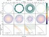Fig. 2 Evolution of a BH embedded in an NFW DM halo, with and without a central stellar bulge, as simulated using the OTIS code. The first three columns correspond to BH trajectories in an NFW halo with initial distance of 20 kpc from the halo centre and orbit ellipticities e = 0, e = 0.5, e = 0.8, while the fourth column includes a central bulge and shows the trajectory of the BH initially at 20 kpc and placed on a circular orbit. In the first and second rows, the trajectory color-code refers to the time elapsed since the beginning of the simulation, as indicated by the color map. Top row: BH trajectories when it is embedded within the static gravitational potential generated by the mass distribution, thus neglecting collisional effects from two-body encounters. Middle row: BH trajectories when collisional effects are included through the analytical description of the DF force (see Eq. (12)). Bottom row: time evolution of the BH’s radial distance from the halo centre. The green line shows the distance when aBH follows Eq. (5) (or Eq. (22) in the last column) mimicing the effect of a BH embedded in a collisionless medium. The purple line adds the DF contribution given by Eq. (12) for eccentricity e = 0, while the distance corresponding to the middle row of each panel is displayed by the orange curve.

3 Numerical simulations

We carried out several simulations with the aim to assess the performances of DF correction at different resolutions, both with and without DF prescriptions to improve the numerical description of BH dynamics. In this section, we describe the specific model that we follow to correct for unresolved DF (Sect. 3.1) and the general simulation setup we adopted in this work (Sect. 3.2). Finally, we introduce the list of simulations in Sect. 3.3, with the results presented in Sect. 4.

3.1 Numerical DF correction

Within the context of N-body simulation codes, the gravity solver already accounts for the DF force, at least within the limits allowed by finite force and mass resolution. However, due to this limited resolution, a correction term needs to be introduced (e.g. Hirschmann et al. 2014; Tremmel et al. 2015). Accordingly, the total acceleration experienced by a BH particles can be expressed as the sum of the contribution computed by the gravity solver, a_grav, and a correction term, a_DF, due to the unresolved dynamical friction, $$a_{BH}=a_{\text{grav\hspace{0.17em}}}+a_{DF}.$$(26)

Throughout this paper, we adopted and refined the model for DF correction introduced by (Damiano et al. 2024, hereafter D24). Following Tremmel et al. (2015), to avoid double-counting the DF contribution already captured by the gravitational solver, we applied DF correction only at distances smaller than a chosen maximum impact parameter, denoted as b_max,c. In line with this, D24 adopt b_max,c = ϵ_BH, where ϵ_BH is the gravitational softening length of the BH particle. In this work, we adopted the same assumption when the BH mass exceeds that of the surrounding DM particles. However, as the BH becomes less massive, we explored alternative values for b_max,c to assess their impact (see Sect. 4.1.2).

Under the assumption that the phase-space density below b_max,c can be approximated as a sum of the discrete contributions from neighbour particles (D24), the DF correction becomes $$\begin{array}{cc}{a}_{\text{DF}}& ={\displaystyle \sum _j^{\text{N}}-2\pi {\text{Gm}}_{\text{j}}\left({\text{M}}_{\text{BH}}+{\text{m}}_{\text{j}}\right){\tilde{\text{n}}}_{\text{j}}}\\ & \times \ln \left[1+\Lambda {\left({\text{m}}_{\text{j}}\right)}^2\right]\frac{v_{\text{j}}-v_{\text{BH}}}{{\left|v_{\text{j}}-v_{\text{BH}}\right|}^3}.\end{array}$$(27)

Here, m_j, v_j are the mass and velocity of the j-th particle, ñ_j is the local number density, and the summation runs over all the N particles that are found within a distance b_max,c from the target BH particle. For completeness, the expression for Λ(mj), consistent with the definition adopted in D24, is reported in Appendix B, as expressed in Eq. (B.29).

Assuming constant density within a sphere of radius b_max,c = ϵ_BH, Eq. (12) reduces to the original formulation of D24 with ${\tilde{n}}_j=3/\left(4\pi {ϵ}_{BH}^3\right)$, $$a_{\text{DF}}=\frac{3}{2{ϵ}_{\text{BH}}{}^3}\underset{\text{N}\left(<{ϵ}_{\text{BH}}\right)}{\overset{\text{j}}{{{\displaystyle \sum }}^{\text{}}}}\text{ln}\left[1+\text{Λ}{\left({\text{m}}_{\text{j}}\right)}^2\right]m_j\left({\text{m}}_{\text{BH}}+{\text{m}}_{\text{j}}\right)\frac{\left(v_{\text{j}}-v_{\text{BH}}\right)}{{\left|v_{\text{j}}-v_{\text{BH}}\right|}^3}.$$(28)

We note that Eq. (27) generalises the formulation of D24 to accommodate different particle masses and non-uniform density around a BH particle. The value and numerical computation of the local number density depends on the specific kernel adopted. After introducing the OpenGADGET3 code used in this work (Sect. 3.2), we detail the calculation of the number density in Sect. 4.1.2.

Interestingly, the DF correction introduced in this work can be formally derived from the first-order diffusion coefficient in the Fokker-Planck equation, derived from the collisional Boltzmann equation to describe the evolution of the phase-space probability density function of a self-gravitating fluid. This connection provides a more rigorous theoretical foundation to our model for DF correction. We defer the full derivation to Appendix B, where we start from the collisional Boltzmann equation and summarise the steps leading to the Fokker-Planck formulation, ultimately showing how our DF correction emerges naturally as the first-order term in the diffusion equation, as previously shown by Rosenbluth et al. (1957), Ipser (1977), and Binney & Tremaine (2011).

3.2 Simulations set up

We generated several realisations having different resolutions of an NFW halo using the MAKEGALAXY code (Springel & White 1999), selecting an NFW DM density profile with a concentration parameter of c = 4.38 and virial mass of M₂₀₀ = 10¹³ M_⊙. This choices, consistent with Genina et al. (2024), ensure that for an orbiting BH of mass 10⁹ M_⊙ with initial halocentric distance r = 20 kpc ≃ 1/4 r_s, the significantly larger mass of the host halo minimises perturbations to the halo density and velocity distributions, preventing artificial alterations in its structure. The halo centre position is calculated using the shrinking sphere algorithm developed by Power et al. (2003).

To explore the effects of DF on the BH in a more complex system, we also carried out an additional set of simulations at varying resolutions, incorporating a central stellar bulge core modeled with a Hernquist profile (see Sect. 2.3). The bulge is characterised by a mass of M_b = 10¹¹ M_⊙ and scale radius r_s = 7 kpc. The simulations are carried out using the OpenGADGET3 code (Groth et al. 2023, D24), which builds upon GADGET3, which is in turn an improved extension of GADGET2 (Springel 2005). The code employs a hybrid tree-particle mesh (TreePM) method to accurately resolve gravitational interactions across different spatial scales. In this approach, long-range gravitational forces are computed using a particle-mesh (PM) method, which efficiently solves Poisson’s equation on a grid, while short-range interactions are handled using a hierarchical tree algorithm, allowing for adaptive force calculations with high resolution in dense regions. When calculating the force softening between particles having different softening lengths, the code adopts the largest softening of the particles among the tree node. This detail is relevant for multi-component system and its effects are further analysed in Sect. 4.2.

3.3 List of simulations

We introduced a BH with a mass of M_BH = 10⁹ M_⊙ at 20 kpc from the halo centre within the halo (eventually complemented with a central stellar bulge) configuration described in the previous sections. By default, BH particles are initialised on a circular orbit around the halo centre, while we also investigate the case of an initially eccentric orbit in Appendix A (see Fig. A.1). Table 1 summarises the full set of simulations performed. From left to right, we report in each column: the specific label assigned to each simulation, the BH to DM particle mass ratio M_BH/M_DM, the BH to stellar mass ratio M_BH/M_∗ (where present), the number of particles used to sample the halo N_Halo, the number of stellar particles used to sample the bulge N_Bulge, the softening of the BH, DM and stellar particles, we indicate whether the simulations adopts the DF correction or not and finally what is the maximum impact parameter adopted in the DF correction.

These simulations are divided into four main subgroups (separated by horizontal lines in Table 1), each designed to examine a specific aspect of the DF correction. In the first set of simulations, we modelled the DM halo using progressively increasing particle numbers (10⁵, 10⁶, 10⁷, 5 · 10⁷). For each realisation of the halo, we evolved the system both including and neglecting the effect of the DF correction of D24 (simulations labelled with ∗_DF_ or ∗_NODF_, respectively). We also adopted two different choices for the softening length: following Power et al. 2003 (hereafter P03) as follows $${ϵ}_{P03}=\frac{4R_{vir}}{\sqrt{N_{vir}}}$$(29) or according to Zhang et al. 2019 (hereafter Z19) as $${ϵ}_{Z19}=\frac{2R_{vir}}{\sqrt{N_{vir}}}$$(30) in simulations labelled with ∗_p03 or ∗_z19 respectively. Before initialising the BH orbit, we verify, that adopting the smaller softening length ϵ_Z19, compared to the standard ϵ_P03, does not alter the density and velocity distributions of the system, which must remain consistent with the analytical predictions. This check is crucial to ensure that no spurious differences in the halo properties, possibly induced by different choices of the softening, affect the subsequent BH dynamics. However, the choice of the softening length not only affects the performance of the N-body gravity solver but also the DF correction. Since we adopt b_max,c = ϵ_BH = ϵ_DM, by decreasing the softening we are also shrinking the region within which we compute the DF correction.

The purpose of this set of simulations is threefold: to assess the performance of the D24 model for DF correction across different resolutions, to test its numerical convergence against resolution, and to study the dependence on the choice of the softening length.

A second set of simulations is devoted to the study of the same configuration but at lower resolution (beginning with LR_) when M_BH < M_DM. Aiming to improve the DF prescription, we test the outcome when enlarging the impact parameter b_max,c to twice the BH softening.

Finally, a third set of simulations is carried out also including a central stellar bulge. We sampled the DM halo with 10⁵, 10⁶, 10⁷ particles and the stellar bulge with 2 · 10⁴, 2 · 10⁵, 2 · 10⁶ particles, respectively. The softening length for the star particles is scaled using the relation $${ϵ}_{\text{*}}={ϵ}_{\text{DM}}{\left(\frac{{\text{M}}_{\text{*}}}{{\text{M}}_{\text{DM}}}\right)}^{1/3}.$$(31)

The BH is initially placed at 20 kpc from the centre, corresponding to approximately three times the bulge scale radius (see Sect. 3.2). As a result, the BH is initially embedded in a DM-dominated environment before gradually sinking into the stellar-dominated core. This raises the question of whether the optimal softening choice for the BH should follow the DM or stellar softening. To address this, we compare two approaches: (i) assigning to the BH the same softening as the DM particles ϵ_BH = ϵ_DM = ϵ_P and (ii) assuming for the BH the same softening of the star particles, ϵ_BH = ϵ_∗, based on Eq. (31).

Both configurations are tested in simulations with and without the DF correction. In cases where DF correction is applied, we adopted b_max,c = ϵ_BH as a reference choice.

Similarly to the second simulation set, but this time including the stellar central bulge, we carried out an additional low-resolution, fourth set of simulations where the BH mass is smaller than the typical DM particle mass M_BH < M_DM. In this setup, we explored both choices of BH softening and, again, we performed two additional tests with increased value of the maximum impact parameter: b_max,c = 2ϵ_∗. It is worth noticing that in all the simulations including the bulge, the BH has a larger mass than the stellar particles, as indicated by the third column in Table 1, even for these low-resolution tests.

4 Results

Throughout this section, we outline the results of the simulations listed in Table 1. We present the results of the different sets of simulations. In Sect. 4.1 we analyse the timescale for sinking of a BH infalling into a DM halo. Sect. 4.2 presents the same results but for a multi-component system composed of a DM halo provided with a central stellar bulge.

4.1 Infalling BH in a DM halo

For all the configurations described in this section, we place a BH of 10⁹ M_⊙ on a circular orbit at 20 kpc from the DM halo centre. Figure 3 shows the trajectories of the BH for simulations with progressively increasing resolution, displayed from left to right, as indicated by the labels below each panel (see Table 1). The orbits are projected in the initial orbital plane and color-coded by time, as shown in the colormap. We note that, regardless of whether the DF correction is applied, the BH develops an eccentric orbit, even if initially placed within a circular orbit, with the eccentricity decreasing as the resolution increases. At the two lowest resolutions, the effect of DF is clearly visible: the BH orbits decays to small halo-centric radii when DF is included, whereas the orbital decay is stalling without DF. In the following subsections, we quantify this behaviour by analyzing the BH–halo centre distance at different resolutions, with particular focus on the lowest-resolution cases (where M_BH < M_DM) discussed in Sect. 4.1.2. The 3D rendered movies of the simulations presented in this section are available for download here³.

4.1.1 Reference resolutions

Figure 4 shows the time evolution of the distance of the BH from the halo centre in different simulations. The left and right columns show simulations where the particle softenings follow Eqs. (29) and (30), respectively. Top panels present the results of simulations without any sub-resolution prescriptions for BH dynamics, while the bottom plots show those where the BH dynamics includes the DF correction from D24. Curves are color-coded according to resolution, with darker shades representing higher resolution. Horizontal, dashed lines indicate the values of the softenings, color-coded according to the resolution of the corresponding simulation. We can visually identify the sinking timescale as the moment when the BH trajectory transitions from a steeper descent to a shallower, flatter curve. Vertical dash-dotted lines mark the sinking timescales hence identified for the three highest resolution simulations. The red line represents the predicted orbit retrieved from OTIS (Sect. 2.4), using a maximum impact parameter b_max of 80 kpc, corresponding to the NFW halo scale radius. In the simulations using the softening ϵ_BH = ϵ_P03, we observe that at lowest resolution and without the DF correction (H1e5_NODF_P03), the BH does not sink toward the halo centre in 10 Gyr. However, when the DF correction is applied at the same resolution, we observe a faster sinking process where the BH crosses its softening scale at ~6 Gyr. For higher-resolution simulations, the BH gradually sinks toward the centre with or without the DF correction. For H1e6_NODF_p03 the sinking timescale is 8.5 Gyr, delayed by about 2 Gyr compared to analytical predictions. At higher resolutions, for H5e7_NODF_p03, the timescale approaches 6 Gyr. As we apply the DF correction, H1e6_DF_p03, H1e7_DF_p03 and H5e7_DF_p03 predict sinking timescales in good agreement with theory, with a timescale for sinking of 6.5 Gyr. Notably, H1e6_DF_p03 achieves the predicted timescale for sinking of H5e7_NODF_p03 but with a 50 times-lower resolution.

Furthermore, H1e7_DF_p03 and H5e7_DF_p03 converge to a sinking timescale of approximately 6 Gyr. For simulations using ϵ_BH = ϵ_Z19 and without the DF correction, the sinking timescale is shorter than in the corresponding simulations with ϵ_BH = ϵ_P03.

When including the DF correction, the results for the three higher resolution simulations align closely with those adopting ϵ_BH = ϵ_P03, thus indicating a weak sensitivity of our DF correction model on the softening choice at these resolutions. On the other hand, H1e5_DF_z19 shows sinking timescales which are in agreement with theoretical expectations, despite the delay shown by the same simulation based on the P03 softening. In summary, the DF correction forces the BH to sink toward the halo centre in the relatively low-resolution runs, while at higher resolution simulations show good agreement with theoretical predictions and resolution convergence. The additional convergence seen when reducing the softening length in line with Z19 indicates that: considering only particles within the ϵ_Z19 softening is sufficient to produce a DF correction that matches the analytical predictions; extending the correction region to ϵ_P03 for the higher resolution cases (where M_BH/M_DM > 70) does not significantly affect the results.

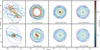Fig. 3 Projected trajectory of the BH in the DM halo on the initial orbital plane, for simulations at progressively increasing resolution, from left to right, as indicated by the labels (see Table 1 for the description of the label of each simulation). Trajectories are color-coded by time, as shown by the colormap.

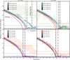Fig. 4 Sinking timescales for a BH initially seeded on a circular orbits within a DM-only NFW halo at 20 kpc from the halo centre. The left and right columns show simulations with softenings derived from Eqs. (29) and (30), respectively. Top plots refer to simulations without any DF correction, while the bottom plots include the DF correction according to D24. Lines are color-coded by resolution, with lighter to darker shades indicating increasing resolution (as shown in the colormap). Horizontal dotted lines represent the softening lengths, and vertical dash-dotted lines mark the sinking timescales for the three highest resolution runs. The red line shows the analytically predicted merging timescale using bmax = 20 kpc.

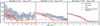Fig. 5 Trajectories of a BH placed on a circular orbit at 20 kpc from the centre of a DM halo for three different halo resolutions. From left to right, the halo is sampled with 104, 105 and 106 particles. The dashed black lines indicate the Plummer-equivalent softening length of each simulation. Orange lines represent the BH trajectory when the DF correction is applied according to Eq. (33), while the blue lines correspond to the original DF correction in Eq. (6) of D24, the red line shows the analytical prediction from OTIS (Sect. 2.4). The ratio of the BH mass to the surrounding DM particle mass is indicated at the top of each panel.

4.1.2 Stability at lower resolutions

All the simulation setups analysed so far have involved BH with a mass larger than the surrounding particles. However, in cosmological simulations, it is common to encounter situations where BHs have masses smaller than nearby DM and star particles, especially short after a BH is seeded. In this case, two-body encounters can spuriously heat the BH motion, resulting in an inaccurate representation of its trajectory. To mitigate possible shortcoming, simulations often couple the DF correction to a boosted dynamical mass unless, so that the mass of the BH entering in the computation of the gravitational force is set to be at least to a value comparable or exceeding the mass of the surrounding particles (Chen et al. 2022). In this section, we describe how our particle-interaction-based approach to correct for the DF overcomes these limitations. In Appendix B, we explain how we derived our DF correction from the Fokker-Planck equation, assuming that potential fluctuations affecting a mass M_BH arise from two-body interactions with a population of particles of mass, m_j. In the formulation of D24, ϵ_BH defines the maximum impact parameter and the density surrounding the BH is assumed to be homogeneous. While this approach does not impose any restrictions on the minimum allowed mass ratio M_BH/m_j, it still struggles to accurately reproduce the sinking timescale for BHs that are less massive than the nearby particles. To address this limitation, we refined the model by relaxing the assumption of a homogeneous surrounding medium. Additionally, we tested the correction by extending the maximum correction region beyond the softening length, namely, using b_max,c > ϵ_BH). In this section, we show how these refinements improve the accuracy of the sinking timescale and ensure that the method remains robust across varying mass regimes, being also reliable when M_BH/m_j < 1.

Starting from the cubic-spline kernel (Monaghan & Lattanzio 1985), expressed as $$W\left(r,ϵ\right)=\frac{8}{\pi {ϵ}^3}\{\begin{array}{ll}1-6{\left(\frac{r}{ϵ}\right)}^2+6{\left(\frac{r}{ϵ}\right)}^3\hfill & ;0\le \frac{r}{ϵ}\le \frac{1}{2},\hfill \\ 2{\left(1-\frac{r}{ϵ}\right)}^3\hfill & ;\frac{1}{2}<\frac{r}{ϵ}\le 1,\hfill \\ 0\hfill & ;\frac{r}{ϵ}>1,\hfill \end{array}$$(32) where ϵ_∗is the softening length, the OpenGADGET3 code derives the spline-softened gravitational force by taking the force from a point mass m to be the one resulting from a density distribution ρ(r) = mW(r, ϵ) (see Springel et al. 2001, Appendix A). Therefore, the local number density from the j-th particle placed at a position r_j in Eq. (12) is ñ_j = W(r_j, ϵ) and Eq. (12) becomes $$\begin{array}{c}{a}_{\text{DF}}=\underset{\text{N}\left(<{\text{b}}_{\text{max},\text{c}}\right)}{\overset{\text{j}}{{{\displaystyle \sum }}^{\text{}}}}-2\pi {\text{Gm}}_{\text{j}}\left({\text{M}}_{BH}+{\text{m}}_{\text{j}}\right)\text{W}\left({\text{r}}_{\text{j}},ϵ\right)\\ \times \text{ln}\left(1+\text{Λ}{\left({\text{m}}_{\text{j}}\right)}^2\right)\frac{{\text{v}}_{\text{j}}-{\text{v}}_{BH}}{{\left|{\text{v}}_{\text{j}}-{\text{v}}_{BH}\right|}^3}.\end{array}$$(33)

Figure 5 shows the results of the application of Eq. (33) instead of Eq. (13), when M_BH < M_DM (left plot) and M_BH > M_DM (central and right plots) for the usual DM halo characteristics and initial BH coordinates described in Sect. 3.2.

The dashed black line corresponds to the Plummer-equivalent softenings ϵ_BH = ϵ_P03 equal to 14.4, 4.44, and 1.44 kpc from the left to the right panel. The orange curve in each plot indicates the trajectory of the BH when the DF correction is applied according to Eq. (33). The blue curve corresponds to the original implementation of D24 (see Eq. (13)). The red line indicates the analytical prediction according to the OTIS library. At the top of each panel, we indicate the ratio of the BH mass to the mass of the surrounding DM particles. In the left plot, where the BH mass becomes smaller than that of nearby particles, using the DF correction adopted in D24, the BH cannot sink to the halo centre but oscillates with a maximum apocentre distance to the centre of the halo higher than the Plummer-equivalent softening. However, at this resolution, refining the description of the surrounding spatial distribution significantly improves the results: the BH sinks well below the Plummer-equivalent softening with timescales in agreement with the analytical results. Even when M_BH > M_DM the refinement shows its success: the delayed sinking process predicted by the DF correction from D24 is now reduced and once again, the improved sinking timescale is in good agreement with the analytical predictions.

Lastly, at higher resolution (right panel) the refinement has a negligible impact on the BH trajectory. The blue and orange trajectories are similar, indicating that the refinement can be applied with the same effectiveness as the original implementation in this regime.

The second refinement that we test involves expanding the region over which the DF correction is applied. At lower resolutions, the assumption that DF effects are already well described by simulations at the resolved scales may no longer hold. To address this limitation, we explored the effect of assuming different values for the maximum impact parameter in the DF correction.

Figure 6 presents the results of these tests. From left to right, each column displays our findings when sampling the DM halo with 5 × 10³, 7 × 10³, 10⁴ particles. In these cases, the BH is less massive than the DM particles, with corresponding mass ratios of M_BH/M_DM = 0.35, 0.5, 0.7. The grey curves represent results obtained without applying the DF correction, while the blue curves illustrate the trajectory of the BH when the DF correction is implemented according to Eq. (33), with b_max,c = ϵ_BH (lighter) or b_max,c = 2ϵ_BH. The analytical solution from OTIS (Sect. 2.4) is shown in red, and the dashed black line indicates the softening length of each simulation.

Across all the resolutions analysed, the DF correction plays a crucial role in confining and driving the BH toward the centre of the halo. Without the DF correction, the BH does not experience any orbital decay, whereas with the correction applied, it sinks well below the softening scale. Although this orbit shrinking occurs below the resolved scales, the process is captured with a timescale that is delayed when M_BH/M_DM = 0.35, 0.5 but aligns with the analytical prediction when M_BH/M_DM = 0.7. However, we highlight that in all these low resolution tests, the BH exhibits considerable orbital scatter, and its trajectory is not circular.

Lastly, increasing the size of the region within which we apply the DF correction does not lead to any significant improvement in the sinking timescale at any resolution. This suggests that particles located below the softening scale contribute most significantly to the DF correction. To validate this result, we further extended the corrective region to b_max,c = 4ϵ_BH and repeated the simulations with the same set-up presented in this section obtaining the same conclusions (see also Sect. 4.2.2).

Based on the tests carried out in this section, we conclude that the DF correction introduced in D24 (see Eq. (13)) is not adequate for accurately modeling the evolution of BHs when their mass is smaller than the mass of the surrounding particles. However, by introducing refinements that relax some of the underlying assumptions in the formula, we can significantly improve these results. Specifically, incorporating a spatially dependent phase-space density (Fig. 5) allows for a more accurate reproduction of the sinking process of BHs, even those lighter than the surrounding DM particles.

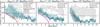Fig. 6 Sinking path of a BH of mass MBH infalling in a DM halo sampled with DM particles of mass MDM such that MBH/MDM < 1. Each column refers to a different halo sampling, with increasing halo resolution from left to right. The grey curve corresponds to the simulation without the DF correction, whereas the blue curve refer to the simulation where the DF correction applied to the BH and computed according to Eq. (33) with bmax,c = 2ϵBH and bmax,c = ϵBH (lighter curve). We report in red the analytical estimation from OTIS. The Plummer-equivalent softening in each simulation is marked with the horizontal dashed line. For the details of each simulation, refer to Table 1.

4.2 Infalling BH in a composite DM and stellar bulge system

In this section, we describe the results for the orbital evolution of a BH embedded in a composite system, made of a DM halo hosting an inner stellar bulge. The initial position of the BH is, as in the previous sections, 20 kpc from the halo centre, and its initial velocity is the circular velocity at this halo-centric distance. Given the scale radius of the bulge is r_b = 7.2 kpc, the BH is initially placed in a DM-dominated region, with its orbit lately decaying into the stellar-dominated core. As anticipated in Sect. 3.2, the OpenGADGET3 code uses, for the interactions between particles with different softenings, the largest softening found for all the particles in each tree node. This is particularly relevant in a multi-softening system as the one presented in this section, where the BH experiences the transition from a DM-dominated to a stellar-dominated regime. To exploit the differences between different choices for ϵ_BH, we carried out simulations where the BH gravitational softening is set to be equal to both the DM, ϵ_BH = ϵ_DM, and stellar particles one, ϵ_BH = ϵ_∗, with ϵ_∗ scales with resolution according to Eq. (31). All the simulations are carried out both with and without the DF correction, using Eq. (33) with b_max,c = ϵ_BH. In Sect. 4.2.2 we investigate the effect of using a larger DF correction region.

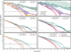Fig. 7 Comparison of the evolution of BH halo-centric distances during the BH sinking for different simulation setups. From the upper to the bottom row we show the results at increasing resolutions. Left column compares simulation using ϵBH = ϵDM or ϵBH = ϵ∗ for simulation with and without the DF correction. The right panels display the results for a BH embedded either in the NFW halo alone (as described in Sect. 3.2) or with the addition of a central stellar bulge. The red curves show the analytical predictions computed with OTIS, with the lighter curve corresponding to the DM-only case and the darker curve including the central bulge. Dashed horizontal lines indicate the Plummer-equivalent softenings used in the simulations, with Z19 softenings marked in black and P03 softenings in grey.

4.2.1 Reference resolutions

Fig. 7 presents the results of these simulations, showing the distance to the system for different runs. The left panels compare simulations with and without the DF correction, as well as with different choices for the BH softening length: for ϵ_BH = ϵ_DM or ϵ_BH = ϵ_∗. The meaning of each label is indicated in Table 1. From top to bottom, we show simulations at increasing resolution. Simulations at lower resolution and without the DF correction, B1e5_NODF_ϵ_DM and B1e5_NODF_ϵ_∗, exhibit the slowest orbital decay, crossing the BH softening length only after ~9 Gyr, with no significant difference for different choices of ϵ_BH. Increasing the number of particles sampling the halo and the bulge as for B1e6_NODF_ϵ_DM, the BH sinking timescale is noticeably delayed when approaching the bulge-dominated region. Interestingly, this effect is less pronounced in B1e6_NODF_ϵ_∗. According to our choice for the force softening – see Sect. 3.2 – in the DM-dominated region, the BH primarily interacts with the DM softening length, leading to a nearly identical trajectory for both softening choices. However, as the BH approaches the bulge scale radius, the impact of softening differences becomes evident: larger softening values lead to longer sinking timescales, consistent with the findings in Sect. 4.1.

Nevertheless, these differences largely vanish when comparing B1e5_DF_ϵ_DM and B1e5_DF_ϵ_∗, thus confirming that the introduction of the DF correction compensates for the different choices of softening. Simulations at higher resolution reinforce these trends, with only a mild deviation observed in B1e7_NODF_ϵ_DM when approaching r_b. However, also in this case, the sinking timescale does not converge in simulations without the DF correction at different resolutions and different choices for the BH softening.

Since the presence of a central stellar component is expected to reduce the sinking timescale (as predicted by analytical estimates, see Fig. 2), it is useful to compare the numerical results with and without the central bulge. The right column of Figure 7 directly compares analogous simulations with and without the stellar bulge, using ϵ_BH = ϵ_DM = ϵ_P03 in both cases, also comparing the versions with and without the DF correction. Interestingly, even when sampling the halo with 10⁷ particles (a configuration that successfully reproduced the results of the infall in the DM only in the case depicted in Fig. 4), the BH exhibits a longer sinking timescale in the presence of a central stellar bulge, an effect that is less pronounced when using the DF correction.

The delay in the BH orbital decay is less pronounced when its gravitational softening length is set equal to that of the stellar particles. This suggests that this effect may be driven by the softened nature of the gravitational interactions. In order to verify this, we carried out two additional tests further reducing the softening lengths to the values ϵ_DM = ϵ_Z19 and ϵ_BH = ϵ_∗, where ϵ_∗ follows Eq. (31). We show the results in Fig. 8, which compares the BH-halo centre distance in two simulations, (one with DF, labelled as DF_LOWSOFT and one without, namely NODF_LOWSOFT), with the same resolution as B1e6_DF_ϵ_*, but using the smaller softening lengths, so that ϵ_DM = 0.72, ϵ_BH = ϵ_∗ = 0.25. We compare the results both with simulations at the same mass resolution but using a larger force softening and the analytical predictions from OTIS. Again, reducing the softening causes a significant delay in the orbital decay. This result highlights that simulations involving multiple particle species are particularly sensitive to softening choices. Deviations from analytic expectations can arise either due to softened gravitational interactions (for overly large softenings) or from numerical heating caused by two-body encounters (for overly small softenings). In both cases, we note that the application of the DF correction partially mitigates these effects.

Interestingly, B1e7_DF_ϵ_∗ delays the sinking process with respect to the lower resolution simulation B1e6_DF_ϵ_∗. To investigate the possible origin for this, we performed several tests with different softening choice and configuration of the initial conditions. Our tests reveal that the discrepancy arises from the specific realisation of the initial conditions that can impact the sinking timescale, with different initial conditions introducing stochastic variations (as already inferred by Genina et al. 2024), although not directly inferred from density or velocity distribution profiles.

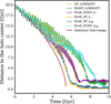Fig. 8 Evolution of the BH–halo centre distance for simulations with the same mass resolution as B1e6_DF_ϵ∗ but using reduced gravitational softening lengths: ϵDM = 0.72, ϵBH = ϵ∗ = 0.25. The green curves show the results from these simulations, with the darker line corresponding to the run without dynamical friction (NODF_LOWSOFT) and the lighter green line including the DF correction (DF_LOWSOFT). For reference, we plot in yellow and purple the outcome of B1e6_DF_ϵ∗ and B1e6_NODF_ϵ∗, while blue curves shows the results from B1e6_NODF_ϵDM (light) and B1e6_DF_ϵDM (dark). The red line represents the analytical predictions from OTIS.

4.2.2 Stability at low resolution

To extend our analysis to systems composed of particles with masses that are higher than the BH mass, we studied the trajectory of the BH under these conditions, in a similar to the approach taken in the study presented in Section 4.1.2. In the previous case, refining the D24 model by incorporating a kernel-dependent number density in Eq. (33) successfully reproduced the sinking process, even at low resolution, but we found no significant improvement when enlarging the corrective region. Given these findings, we conducted a comparable set of tests in the configuration that also includes a bulge component. The results of these simulations are presented in Figure 9, where we examine the evolution of the BH distance from the halo centre across different simulation settings.

The figure compares cases without the DF correction either when ϵ_BH = ϵ_DM or ϵ_BH = ϵ_∗ (lighter and darker green curves), to those where the DF correction is applied using different impact parameters. We show the outcomes of simulations where b_max,c = ϵ_BH in purple, with the darker line corresponding to ϵ_BH = ϵ_DM and the lighter one to ϵ_BH = ϵ_∗. We then increased the maximum impact parameter to b_max,corr = 2ϵ_BH = 2ϵ_∗ (dark orange) and b_max,corr = 4ϵ_BH = 4ϵ_* (light orange).

When the DF correction is not included, the BH orbit does not decay, regardless of the softening choice. However, once the correction is acting, the BH sinks to the centre, again showing no dependence on the adopted BH softening. Notably, increasing the maximum impact parameter results in an accelerated sinking process. Ultimately, enlarging beyond ϵ_BH the region within which the DF is corrected region does not improve the performances of the model in the DM halo-only case, while leading to an overestimation of the DF in a multi-component system, eventually producing too short sinking timescales compared to analytical predictions.

4.2.3 Contributions to the DF acceleration

In a system composed of both DM and stellar components, it is interesting to examine the relative importance of different terms in our model to correct the DF and, in particular, to assess the separate contributions of stars and and of DM to the overall DF correction.

Fig. 10 presents the analysis of these different components entering Eq. (12) for simulation LR_B1e4_DF_ϵ_∗, B1e5_DF_ϵ_∗ and B1e6_DF_ϵ_∗,B1e7_DF_ϵ_∗. The first panel from the top shows the evolution of the BH distance to the halo centre, followed by the relative strength of the DF acceleration compared to the gravitational acceleration (second panel). The third panel illustrates the relative contributions of stars and DM to the total DF correction, while the fourth panel shows the number of particles enclosed within ϵ_BH (hence contributing to the DF correction). The last two panels report the value of log(1 + Λ²) and the term $1/{\text{v}}_{\text{rel\hspace{0.17em}}}^3$, $$\frac{1}{{\text{v}}_{\text{rel}}^3}=\underset{\text{N}\left(<{ϵ}_{\text{BH}}\right)}{\overset{\text{i}}{{{\displaystyle \sum }}^{\text{}}}}\frac{1}{{\left({\text{v}}_{\text{i}}-{\text{v}}_{\text{BH}}\right)}^3}.$$(34)

The horizontal dashed lines in the top panel mark the softening values color-coded according to the simulation they refer to.

As illustrated in the second row, a notable feature of these results is the enhanced DF correction at lower resolutions. With increasing resolution, DF is more accurately captured by the gravitational solver, reducing the need for an explicit DF correction, which consequently becomes progressively weaker. This effect is naturally accounted for in the prescription adopted, thus demonstrating that convergence to the analytical predictions can be achieved already at relatively low resolution. The relative contribution of the stellar component to DF also increases as the BH approaches the bulge-dominated region, except in the lowest-resolution simulation, where the softening is so high to already account for the entire stellar mass enclosed within the bulge from previous times in the simulation. This effect is further reflected in the number of particles within ϵ_BH, which remains constant at the lowest resolution but increases for higher-resolution cases. Remarkably, the higher is the number of particles contributing to the DF correction, the lower is the relative velocity between the BH and the surrounding medium, leading to an increase of the velocity contribution in Eq. (33).

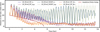Fig. 9 Evolution of the BH’s distance from the halo centre in low-resolution simulations including both a DM halo and a stellar bulge. The figure compares different setups: no DF correction (lighter and darker lines for different softening choices), DF correction with bmax,c = ϵBH and ϵBH = ϵDM or ϵBH = ϵ∗(lighter and darker purple lines), and DF correction with an extended impact parameter bmax,c = 2ϵBH, 4ϵBH (lighter and darker orange lines). The brown curve represents the analytical sinking timescale from OTIS.

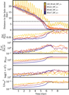Fig. 10 Breakdown of the different contributions to the DF correction term in Eq. (12) for simulations LR_B1e4_DF_ϵ∗, B1e5_DF_ϵ∗, B1e6_DF_ϵ∗, and B1e7_DF_ϵ∗. From top to bottom: BH distance to the halo centre, ratio of DF acceleration to gravitational acceleration, ratio of stellar to DM contributions to DF, total number of particles within ϵBH, Coulomb logarithm term, and inverse velocity term of Eq. (34).

5 Discussion

In this work, we compared analytical predictions (Sect. 2) and numerical simulations (Sect. 3) of the sinking timescale for a BH infalling into a DM halo, both with and without a central stellar bulge. The analytical results were computed using OTIS python library to numerically solve the equations of motion of the BH (Sect. 2.4). Using the OpenGadget3 code, we simulated the BH inspiralling onto the halo, exploring a wide range of resolutions and different softening choices. We applied a refined prescription to correct for unresolved DF, which extends the original D24 model, and extensively tested its impact on the BH dynamics.

Figure 11 summarises some of our key findings of our analysis. In both panels, we plot the sinking timescales as a function of the total number of particles in the halo, when the BH is embedded in a pure DM NFW halo (left panel) or when a stellar Hernquist bulge is also included (right panel). Symbols represent different simulation setups: circles and diamonds indicate simulations with and without DF correction, respectively. The horizontal red dashed line marks the analytical sinking timescale predicted by OTIS. In the right panel, teal-edged points correspond to simulations where the BH softening matches the DM particle softening (ϵ_BH = ϵ_DM), while black edges correspond to simulations where ϵ_BH = ϵ_∗. The color of each point encodes the mean eccentricity of the BH during its inspiraling. The eccentricities were calculated by identifying local maxima and minima in the BH distance to the halo centre (apocentre r_apo and pericentre r_peri) and computing the eccentricity for each orbit as $$e=\frac{r_{\text{apo}}-r_{\text{peri}}}{r_{\text{apo}}+r_{\text{peri}}}.$$(35)

We then averaged the eccentricity over all orbits to obtain the color-coded value shown in the colorbar.

In the left panel, we observe that without the DF correction the BH experiences significantly longer sinking timescales. In low-resolution runs, they often even fail to sink, as discussed in Sect. 4.1.2. Reducing the gravitational softening shortens the sinking time even without DF, but this effect remains insufficient to fully recover the analytical prediction. On the other hand, applying the DF correction produces sinking timescales that closely match the analytical predictions across all resolutions, and most importantly, reduces the sensitivity on the specific softening choice, as explained in Sect. 4.1.

The inclusion of a stellar bulge, as depicted in the right plot, adds complexity to the BH sinking process. In principle, the higher central density contributed by the bulge, should accelerate the BH decay. However, our simulations reveal that numerical heating – especially at low resolution – counteracts this effect, thereby delaying the BH infall. Simulations without DF correction show pronounced deviations from analytical predictions, particularly at low resolutions. Quite remarkably, the application of the DF correction mitigates these numerical effects. Moreover, Fig. 10 illustrates that the DF correction is most significant in the dense central regions, where the relative velocity between the BH and surrounding particles decreases. In these conditions, the DF correction can contribute up to ~10% of the total gravitational acceleration. As already pointed out by Genina et al. (2024), the dynamical heating of the BH induced by the numerical resolution not only affects the sinking timescale but also the orbital eccentricity. Figure 11 shows that the lower the resolution the higher is the mean orbital eccentricity. Even initially placing the BH on a circular orbit, it acquires a mean eccentricity reaching up to ~0.5 at lower resolution. In this case, the addition of the DF correction only slightly mitigates this effect at low resolution.

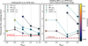Fig. 11 BH sinking timescale as a function of the total number of particles in the halo, for a pure DM NFW halo (left) and for a DM halo with a central Hernquist bulge (right). Diamonds indicate simulations without DF correction, circles indicate simulations with DF correction. The horizontal red dashed line shows the analytical sinking timescale from OTIS. In the left panel, teal-edged points, connected by teal dashed lines, adopt softening from Eq. (30), black-edged points connected by black dashed lines are for the softening from Eq. (29). In the right panel, teal edges and teal dashed lines correspond to ϵBH = ϵDM, while black edges with black dashed lines correspond to ϵBH = ϵ∗. The color of each point indicates the BH orbital eccentricity, as highlighted in the colorbar.

6 Conclusions

In this paper, we present results from our analysis of controlled numerical experiments aimed at describing the infall of a black hole (BH) into a dark matter (DM) halo, both with and without the inclusion of a central stellar bulge. The purpose of this analysis was to address the following key concerns: (i) characterising the impact of an additional dynamical friction (DF) correction to the BH gravitational acceleration in controlled numerical simulations; (ii) considering whether the sinking timescale obtained with the DF correction converges at a progressively increasing resolution; (iii) how well the numerical results agree with analytical predictions at different resolutions; (iv) examining the impact of a stellar bulge on BH dynamics; (v) and investigating whether a DF correction can effectively model BH sinking toward the halo centre, even in the unfavorable case when the BH mass is smaller than the surrounding particle masses.

To properly address these issues, we combined analytical calculations and numerical simulations at varying resolution. As for the analytical approach, outlined in Sect. 2, we developed the OTIS library⁴ to solve the equations of motion of an inspiralling BH in an NFW halo, optionally including a stellar bulge. As for the numerical approach, we used the N-body TreePM code OpenGadget3 to simulate the sinking of a BH initially placed at 20 kpc from the centre of the halo. The DF correction applied consist of a refined version of the prescription introduced in Damiano et al. (2024), by incorporating a kernel-weighted estimate of the local density surrounding the BH, described in Sect. 3.1 and 4.1.2. From this study, we have drawn the following main conclusions:

• Impact of the DF correction and numerical convergence: the addition of the DF correction significantly reduces the BH sinking timescale compared to the cases of uncorrected DF. The results converge at increasing resolution, thus confirming the robustness of the implementation (see Sect. 4.1, Fig. 4);

• Comparison with analytical predictions: simulations with the DF correction closely match the analytical expectations. In contrast, simulations without DF correction show that the BH fails to sink at low resolution or exhibits significant delays ranging from 2 Gyr to 500 Myr depending on resolution (see Sect. 4.1, Fig. 4);

• Impact of the stellar bulge: in contrast to what is expected from analytical predictions, the inclusion of a stellar bulge delays the sinking process in numerical simulations that are either due to softened interactions or numerical heating. However, the DF correction is able to mitigate this effect. We find that the stellar contribution to DF becomes significant (up to 10%) in the central stellar core (see Sect. 4.2, Figs. 7 and 10);

• Stability at low resolution: the refined DF model allows us to accurately track the BH inspiralling orbits even when the BH mass is lower than that of surrounding particles, comprising a challenging regime for standard N-body simulations and typical of cosmological simulations. (see Sect. 4.1.2, 4.2.2, Figs. 5 and 9).

As a general conclusion, our study demonstrates that the refined DF implementation, besides having a solid theoretical foundation (see Appendix B), also yields reliable results at high resolution and successfully models BH dynamics, even in the critical low-mass regime. This holds key implications in view of its application to cosmological simulations: reliable BH tracking is essential to accurately model BH-galaxy co-evolution, since BH motion affects gas accretion, the deposition of the ensuing active galactic nucleus (AGN) feedback energy, and, hence, the subsequent evolution of the host galaxy. Moreover, our ability to model BH sinking in low-resolution regimes opens the door to carry out larger volume simulations, which are crucial for building statistically robust predictions of gravitational wave event rates for current and future facilities such as PTA (e.g. Hobbs et al. 2010) and LISA (e.g. Colpi et al. 2024).

Acknowledgements

AD gratefully acknowledges the University of Zurich for hosting part of this research, and thanks Pedro Capelo and Lucio Mayer for their valuable feedback and insightful discussions. Simulations were performed at the CINECA Supercomputing Center (Bologna, Italy) with computing time allocated through national and CINECA-UNITS agreements, as well as at the INAF – Astronomical Observatory of Trieste PLEIADI cluster (Bertocco et al. 2020; Taffoni et al. 2020). This paper has been supported by: the Fondazione ICSC, Spoke 3 Astrophysics and Cosmos Observations. National Recovery and Resilience Plan (Piano Nazionale di Ripresa e Resilienza, PNRR) Project ID CN_00000013 “Italian Research Center on High-Performance Computing, Big Data and Quantum Computing” funded by MUR Missione 4 Componente 2 Investimento 1.4: Potenziamento strutture di ricerca e creazione di “campioni nazionali di R&S (M4C2-19 )” – Next Generation EU (NGEU); by the National Recovery and Resilience Plan (NRRP), Mission 4, Component 2, Investment 1.1, Call for tender No. 1409 published on 14.9.2022 by the Italian Ministry of University and Research (MUR), funded by the European Union – NextGenerationEU– Project Title “Space-based cosmology with Euclid: the role of High-Performance Computing” – CUP J53D23019100001 – Grant Assignment Decree No. 962 adopted on 30/06/2023 by the Italian Ministry of Ministry of University and Research (MUR); by the INFN InDark Grant. This work was also supported by the Ministry of Education, Youth and Sports of the Czech Republic through the e-INFRA CZ (ID:90254).

References

Appendix A Infalling of a BH on an orbit with initial eccentricity

The initial angular momentum of the BH decreases as we decrease its initial velocity, while keeping its initial position unchanged. According to Eq. (18), this leads to an increase of the orbital eccentricity. In Sect. 2 we demonstrated that for eccentric orbits, the DF has two effects: it circularises the orbit as it approaches the centre, and shortens sinking timescales as eccentricity rises. Here we examine how effectively the DF correction captures these effects across different resolution levels.

Figure A.1 shows the BH distance from the halo centre for an initial position of 20 kpc with varying orbital eccentricities: e = 0.3, e = 0.5, e = 0.8 in the first, second and third column, respectively. Each row shows the results of simulations with a different sampling of the same NFW halo, where resolution increases from top to bottom: N_part = 10⁵ in the first, 10⁶ in the second, 10⁷ in the third and 5 · 10⁷ in the fourth row (the same halo realisations discussed in Sect. 4.1). Yellow and red lines indicate results from simulations using softening length according to P03 (see Eq. (29)) or Z19 (see Eq. (30)), respectively. Analytical expectations from OTIS (see Sect. 2.4) are shown as blue lines, obtained by setting b_max = r_s = 80 kpc. Dotted lines represent the softening values of each resolution for P03 (yellow edge) and Z19 (red edge). All simulations incorporate the DF correction from D24 reported in Eq. (13). When sampling the halo with 10⁵ particles, variations on the BH orbit with the eccentricity are more evident before the BH crosses the softening length value. Within the first 2 Gyrs, the orbits are more eccentric compared to the analytical predictions for e = 0.3 and less eccentric for e = 0.8. Switching from P03 to Z19 softening further reduces the distance to the halo centre due to the lower softening value of Z19. However, at low resolution, distinguishing different orbits according to their eccentricities is not possible; even though the BH is bound within the softening range around the halo centre, no clear trend of the sinking timescale with increasing eccentricity is detectable.

At higher resolutions, results from simulations align more closely with theoretical predictions and the sinking timescale becomes more sensitive to the initial orbital eccentricity. For simulations employing N_part = 10⁶ and 10⁷ particles, numerical results increasingly approximate analytical expectations as eccentricity rises. Sinking timescales from simulation based on the from P03 softenings are slightly delayed compared to those employing the Z19 softenings.

Appendix B A Fokker-Plank based derivation of the DF correction

In this appendix, we demonstrate that our model for the DF correction introduced in Eq. (27) can be recovered as the first-order diffusion coefficient of the Fokker–Planck equation to describe the collision term in the Boltzmann equation for a self-gravitating fluid. Our derivation follows primarily those presented by Rosenbluth et al. (1957), Ipser (1977), and Binney & Tremaine (2008) (see in particular their Appendix L). For clarity, we start by briefly reviewing the derivation of the Fokker–Planck approximation, before demonstrating how the DF expression arises from its first-order term.

Appendix B.1 The Fokker-Plank approximation

Let us consider a stellar system described by the phase-space distribution function f (x, υ, t) , where x and υ denote the spatial and velocity vectors of the stars composing the system. Under the influence of an external force F, and assuming each all stars have the same mass m, the Boltzmann equation is expressed as $$\frac{df}{dt}=\frac{\partial f}{\partial t}+v^j\frac{\partial f}{\partial x^j}+\frac{F^j}{m}\frac{\partial f}{\partial v^j}={\left(\frac{\partial f}{\partial t}\right)}_{\text{coll}}.$$(B.1)

Here, the index j runs over the velocity components (i.e. j = 1, 2, 3) and the collision term on the right-hand side accounts for changes in the distribution function due to stellar encounters. This term is neglected under the assumption that all stars are subject to a smooth potential, so that the Boltzmann equation becomes a continuity equation in phase space. However, in a discretised system of gravitationally interacting particles, collisions among pairs of particles add on top of the action of the smooth potential. The cumulative effect of such interactions generates the collisional effect of a dynamical friction (DF) force.

Under the assumption that the rate of change induced by these encounters is typically much smaller than that caused by the external force, we can assume that within the small phase-space element ∆w = (∆x, ∆υ) and over a short time ∆t, the external field remains constant.

Let w be the phase-space coordinate of a star at time t. Let us also introduce the quantity ψ(w, ∆w) which is defined so that ψ(w, ∆w) d⁶(∆w)∆t is the probability that a star with coordinates w is scattered within the time interval ∆t to the coordinate w+∆w as a result of an encounter. The phase-space distribution function within this volume then changes due to particles that are scattered either into or outside the 6D volume element ∆w. The loss term (contribution from particles scattered out) is $$\frac{\partial f}{\partial t}=-f\left(w\right){{\displaystyle \int }}^{\text{}}{d}^6\text{Δ}w\psi \left(w,\text{Δ}w\right),$$(B.2) while the gain term (contribution from particles scattered in) is $$\frac{\partial f}{\partial t}={{\displaystyle \int }}^{\text{}}{d}^6\text{Δ}w\psi \left(w-\text{Δ}w,\text{Δ}w\right)f\left(w-\text{Δ}w\right).$$(B.3)

Combining the two terms above, the collisional term in Eq. (B.1) can be expressed as $$\frac{df}{dt}={{\displaystyle \int }}^{\text{}}{d}^6\text{Δ}w\left[\psi \left(w-\text{Δ}w,\text{Δ}w\right)f\left(w-\text{Δ}w\right)-\psi \left(w,\text{Δ}w\right)f\left(w\right)\right].$$(B.4)

According to the Fokker-Plank approximation, particle-particle encounters are assumed to be ’weak’, meaning that |∆w| is small, so that we expand the first term in the square brackets of Eq. (B.4) in a Taylor series up to the second order, as $$\begin{array}{l}\psi \left(w-\text{Δ}w\right)f\left(w-\text{Δ}w\right)=\psi \left(w,\text{Δ}w\right)f\left(w\right)\hfill \\ -\underset{6}{\overset{\mu =1}{{{\displaystyle \sum }}^{\text{}}}}\frac{\partial }{\partial w_{\mu }}\left[\psi \left(w,\text{Δ}w\right)f\left(w\right)\right]\text{Δ}{w}_{\mu }\hfill \\ +\frac{1}{2}\underset{6}{\overset{\mu ,v=1}{{{\displaystyle \sum }}^{\text{}}}}\frac{{\partial }^2}{\partial w_{\mu }\partial w_v}\left[\psi \left(w,\text{Δ}w\right)f\left(w\right)\right]\text{Δ}{w}_{\mu }\text{Δ}{w}_v,\hfill \end{array}$$(B.5) where the indices µ and ν run over the phase-space components, i.e. both spatial and velocity coordinates. Substituting this into Eq. (B.4), we obtain $$\frac{df}{dt}=-\underset{6}{\overset{\mu =1}{{{\displaystyle \sum }}^{\text{}}}}\frac{\partial }{\partial w_{\mu }}\left[D\left[\text{Δ}{w}_{\mu }\right]f\left(w\right)\right]+\frac{1}{2}\underset{6}{\overset{\mu ,v=1}{{{\displaystyle \sum }}^{\text{}}}}\frac{{\partial }^2}{\partial w_{\mu }\partial w_v}\left[D\left[\text{Δ}{w}_{\mu }\text{Δ}{w}_v\right]f\left(w\right)\right],$$(B.6) where we defined: $$D\left[\text{Δ}{w}_{\mu }\right]={{\displaystyle \int }}^{\text{}}{d}^6\text{Δ}w\psi \left(w,\text{Δ}w\right)\text{Δ}{w}_{\mu },$$(B.7) $$D\left[\text{Δ}{w}_{\mu }\text{Δ}{w}_v\right]={{\displaystyle \int }}^{\text{}}{d}^6\text{Δ}w\psi \left(w,\text{Δ}w\right)\text{Δ}{w}_{\mu }\text{Δ}{w}_v.$$(B.8)

Eqs. (B.7) and (B.8) are often referred to as the first- and second-order diffusion coefficients. Hereafter, we proceed under the assumption that the encounters are not only weak, but also local. In this case, the dominant contribution to the phase-space shift of a particle arises from interactions with nearby particles. If the encounters are local, the diffusion coefficients can be expressed purely as a function of the velocity shift ∆υ, as in Binney & Tremaine (2008), namely, $$D\left[\text{Δ}{v}_i\right]={{\displaystyle \int }}^{\text{}}{d}^6\text{Δ}v\psi \left(v,\text{Δ}v\right)\text{Δ}{v}_i,$$(B.9) $$D\left[\text{Δ}{v}_i\text{Δ}{v}_j\right]={{\displaystyle \int }}^{\text{}}{d}^6\text{Δ}v\psi \left(v,\text{Δ}v\right)\text{Δ}{v}_i\text{Δ}{v}_j.$$(B.10)

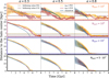Fig. A.1 BH distance from the halo centre over time, starting from an initial position at 20 kpc, with orbital eccentricities e = 0.3, 0.5, 0.8 shown in the first, second, and third columns, respectively. Each row represents a different halo resolution: Npart = 105, 106, 107, 5 · 107 from top to bottom. Yellow lines show results for simulations with P03 softening lengths, and red lines indicate Z19 softenings. Analytical predictions for each orbital eccentricity are represented as a blue line. Dotted lines mark softening values for each resolution (yellow edge for P03, red edge for Z19). All simulations apply the DF correction from D24.

In what follows, we focus on the first-order diffusion coefficient of Eq. (B.9) which is the average change in velocity due to the encounters per unit time. Hence, this term captures the drift of the particle in velocity space and is related to the DF correction we applied. The second-order diffusion coefficient, on the other hand, describes the random scattering of the particle’s velocity, representing the diffusive spread caused by these interactions. We expect that this term becomes important in the low-resolution regime, where stochastic fluctuations dominate. In the analysis presented in this paper we concentrated on the dynamical friction term, associated with the first-order diffusione coefficient. We defer to a future analysis a careful assessment of the ramdom-noise contribution associated with the second-order diffusion coefficient.

Before showing how the first-order coefficient relate to the DF acceleration, we review few basic results of two-body scattering.

Appendix B.2 Two-body scattering

Let us assume to have two particles of mass m and M scattering with impact parameter b and initial relative velocity υ₀. The particle of mass M, because of the interaction with m, experiences a deflection of its trajectory by an angle θ which is related to the impact parameter b by the following expression (Binney & Tremaine 2008), expressed as $$\text{tan}\left(\frac{\theta }{2}\right)=\frac{G\left(M+m\right)}{v_o^{2}b}.$$(B.11)

Therefore, the impact parameter corresponding to a 90° deflection is $$b_{90}=\frac{G\left(M+m\right)}{v_0^2}.$$(B.12)

The intial velocity υ₀ of particle M changes as a consequence of the encounter. The change in velocity ∆υ can be decomposed in a parallel and an orthogonal component to the intial relative velocity υ₀, namely ∆υ_∥ and ∆υ_⊥. Again, following Binney & Tremaine (2008), such components can be written as $$\left|\text{Δ}{v}_{\perp }\right|=v_0\frac{m}{m+M}\text{sin}\theta =\frac{2m{v}_0}{M+m}\frac{b/b_{90}}{1+b^2/b_{90}^2},$$(B.13) $$\left|\text{Δ}{v}_{\Vert }\right|=v_0\frac{m}{m+M}\left(1-\text{cos}\theta \right)=\frac{2m{v}_0}{M+m}\frac{1}{1+b^2/b_{90}^2}.$$(B.14)

When extending the analysis to a system populated by many particles, we can derive the differential scattering cross section for the encounters. Particles scattering from an annular region of area dσ = 2πbdb are deflected into an angular annulus of area 2πR sin(θ)Rdθ within the solid angle dΩ = 2π sin θdθ. Therefore, the differential scattering cross section dσ/dΩ, using Eq. (B.11), can be written as $$\frac{d\sigma }{d\text{Ω}}=\frac{b}{\text{sin}\left(\theta \right)}\frac{db}{d\theta }=\frac{G\left(M+m\right)b}{2\text{sin}\left(\theta \right)v_0^2{\text{sin}}^2\left(\theta /2\right)}.$$(B.15)

Using now Eq. (B.11) for b and sin(θ) = 2 sin(θ/2) cos(θ/2) we obtain $$\frac{d\sigma }{d\text{Ω}}={\left[\frac{G\left(M+m\right)}{2v_0^2{\text{sin}}^2\left(\theta /2\right)}\right]}^2={\left[\frac{b_{90}}{2{\text{sin}}^2\left(\theta /2\right)}\right]}^2,$$(B.16) where b₉₀ is defined in Eq. (B.12).

Based on the formalism introduced in this paragraph, we can go on to derive the DF correction term from the first-order diffusion coefficient of Eq. (B.9).

Appendix B.3 DF correction from the first order diffusion coefficient

Here, we consider different populations of particles with masses m, each described by a corresponding phase-space distribution function f_m(υ). The mean rate of change of velocity for a particle of mass M moving at velocity υ, denoted as D[∆V_i], is given by the cumulative effect of encounters with all m-mass particles. Following the formalism of Rosenbluth et al. (1957), Eq. (B.9) can be rewritten using the differential scattering cross section as: $$D\left[\text{Δ}{V}_i\right]={\displaystyle \sum }_m{{\displaystyle \int }}^{\text{}}{d}^3{v}^{\prime }{f}_m\left(v^{\prime }\right){{\displaystyle \int }}^{\text{}}d\text{Ω}\frac{d\sigma \left(v_0,\theta \right)}{d\text{Ω}}{v}_0\text{Δ}{v}_i^{\text{'}},$$(B.17) where υ₀ = υ − V is the relative velocity between the background particle m and the test particle M, and dΩ = 2π sin θdθ is the solid angle element. Rosenbluth et al. (1957) solved the integral over the angular coordinate in Eq. (B.17) by selecting a convenient reference frame. They defined an orthonormal basis $\left({\widehat{e}}_1^{\text{'}},{\widehat{e}}_2^{\text{'}},{\widehat{e}}_3^{\text{'}}\right)$ such that υ₀ lies along ${\widehat{e}}_1^{\text{'}}$, i.e. $v_0\cdot {\widehat{e}}_1^{\text{'}}=\left|v_0\right|\equiv v_0$. Starting from any fixed orthonormal basis (ê₁, ê₂, ê₃) we have $${\widehat{e}}_i\cdot {\widehat{e}}_1^{\text{'}}=v_{0,i}/v_0.$$(B.18) where v_0,i is the i-th component of υ₀ in the base (ê₁, ê₂, ê₃).

Denoting by ϕ the angle between the orbital plane and the versor ${\widehat{e}}_2^{\text{'}}$, and following the sign convention of Binney & Tremaine (1987) to ensure that the velocity change is positive when the force between the particles is attractive, as in the case of the gravitational force, we can express the change in velocity in the $\left({\widehat{e}}_1^{\text{'}},{\widehat{e}}_2^{\text{'}},{\widehat{e}}_3^{\text{'}}\right)$ reference frame as $$\text{Δ}v=\text{Δ}{v}_{\Vert }{\widehat{e}}_1^{\text{'}}+\text{Δ}{v}_{\perp }\text{cos}\left(\varphi \right){\widehat{e}}_2^{\text{'}}-\text{Δ}{v}_{\perp }\text{sin}\left(\varphi \right){\widehat{e}}_3^{\text{'}},$$(B.19) where ∆v_∥ and ∆v_⊥ are the parallel and perpendicular components of the velocity change relative to υ₀ (and hence to ${\widehat{e}}_1^{\text{'}}$), as introduced in Eqs. (B.14) and (B.13). Furthermore, in the generic reference frame with basis vectors (ê₁, ê₂, ê₃), the components ∆v_i can be expressed as $$\text{Δ}{v}_i=\left(\text{Δ}v\cdot {\widehat{e}}_k^{\text{'}}\right)\left({\widehat{e}}_i\cdot {\widehat{e}}_k^{\text{'}}\right).$$(B.20)

Assuming that the m-populations are isotropically distributed in space, we can average over the angle ϕ. Since 〈cos ϕ〉_ϕ = ⟨sin ϕ⟩_ϕ = 0, the second and third terms in Eq. (B.19) vanish upon averaging. Combining Eqs. (B.19) and (B.20), we obtain $$\text{Δ}{v}_i=\text{Δ}{v}_{\Vert }\left({\widehat{e}}_i\cdot {\widehat{e}}_1^{\text{'}}\right),$$(B.21) so that Eq. (B.17) becomes $$D\left[\text{Δ}{V}_i\right]={\displaystyle \sum }_m{{\displaystyle \int }}^{\text{}}d{v}^{\prime }{f}_m\left(v^{\prime }\right){{\displaystyle \int }}^{\text{}}d\text{Ω}\frac{d\sigma \left(v_0,\theta \right)}{d\text{Ω}}{v}_0\text{Δ}{v}_{\Vert }\left({\widehat{e}}_i\cdot {\widehat{e}}_1^{\text{'}}\right).$$(B.22)

Using then Eq. (B.16) and (B.18), we can write the diffusion coefficient as $$\begin{array}{c}D\left[\text{Δ}{V}_i\right]=2\pi {\displaystyle \sum }_m{{\displaystyle \int }}^{\text{}}{d}^3{v}^{\prime }{f}_m\left(v^{\prime }\right){\left[\frac{b_{90}}{2}\right]}^2{v}_0{v}_{0_i}\times \\ \underset{{\theta }_{\text{min}}}{\overset{{\theta }_{\text{max}}}{{\displaystyle \int }}}\frac{\text{sin}\theta }{{\text{sin}}^4\left(\theta /2\right)}\left(1-\text{cos}\theta \right)d\theta .\end{array}$$(B.23)

In principle, the integration should run over the total solid angle. However, we introduced the integration extremes θ_min, θ_max that, according to Eq. (B.11) correspond to the scattering angle from a maximum and a minimum impact parameter. We adopt b_min = b₉₀ and b_max = ϵ_BH. The parameter ϵ_BH is the gravitational softening length of the BH and serves to account for unresolved, sub-resolution diffusion effects, as discussed in Sect. 3.1. Focusing on the integral over the angular coordinate, it can be easily solved noticing that: sin⁴(θ/2) = (1 − cos θ)²/4 so that $$\begin{array}{c}\underset{{\theta }_{\text{min}}}{\overset{{\theta }_{\text{max}}}{{\displaystyle \int }}}\frac{\text{sin}\theta }{{\text{sin}}^4\left(\theta /2\right)}\left(1-\text{cos}\theta \right)d\theta =\underset{{\theta }_{\text{min}}}{\overset{{\theta }_{\text{max}}}{{\displaystyle \int }}}\frac{4\text{sin}\theta }{1-\text{cos}\left(\theta \right)}d\theta \\ =4\text{ln}\left(1-\text{cos}\theta \right){|}_{{\theta }_{\text{min}}}^{{\theta }_{\text{max}}}.\end{array}$$(B.24)

Moreover, from Eq. (B.14) we have: $$1-\text{cos}\theta =\frac{2}{1+b^2/b_{90}^2}.$$(B.25)

Using the results of Eqs. (B.24) and (B.25) and the minimum impact parameter as b_min = b₉₀ defined in Eq. (B.12) we get $$D\left[\text{Δ}{V}_i\right]=2\pi {\displaystyle \sum }_m{{\displaystyle \int }}^{\text{}}{d}^3{v}^{\prime }{f}_m\left(v^{\prime }\right)\frac{G^2\left(M+m\right)m}{v_0^3}\text{ln}\left(1+\frac{b_{\text{max}}^2}{b_{90}^2}\right)v_{0_i}.$$(B.26)

We can now assume to have a single population of "stellar" particles of mass mj within a spherical region of radius ϵ_BH whose phase-space density distribution is described by the expression $$\text{f}\left(v\right)={\displaystyle \sum }_{\text{j}}{\tilde{\text{n}}}_j\delta \left(v-v_j\right),$$(B.27) where the index j runs over all the particles in the population. In our description of the sub-resolution correction of the DF force, these are the ’neighbours’ of the BH particle, that lie within the BH smoothing length. Using Eq. (B.27) for the phase-space distribution function and b_max = ϵ_BH, Eq. (B.26) becomes $$D\left[\text{Δ}{V}_i\right]=2\pi \underset{j}{{{\displaystyle \sum }}^{\text{}}}\widetilde{n_j}\frac{G^2\left(M+m_j\right)m_j}{{\left|v_j-v\right|}^3}\text{ln}\left(1+\frac{{\left(v_j-v\right)}^4{ϵ}_{\text{BH}}^2}{{\left[G\left(M+m_j\right)\right]}^2}\right)\left(v_{i,j}-V_i\right).$$(B.28)

Following the definition adopted in D24, we write $$\text{Λ}\left(m_j\right)=\frac{{\left(v_j-v\right)}^2{ϵ}_{\text{BH}}}{G\left(M+m_j\right)},$$(B.29) which allows us to recognise that Eq. (B.28) is formally equivalent to the correction term introduced in Eq. (27).

As a final remark, it is important to stress that the first-order diffusion coefficient can be interpreted as an acceleration. This ultimately justifies the fact that the above expression for the diffusion coefficient corresponds to the DF correction of Eq. (27). As pointed out when we introduced it in Eq. (B.9), this coefficient represents the average rate of change of the velocity–already suggesting its physical meaning as an acceleration. However, Rosenbluth et al. (1957) provided an elegant formulation that explicitly demonstrates how this drift term can be related to a force. Following their approach, we consider Eq. (B.26), restricting for clarity to a single stellar population of mass m, so that the summation reduces to a single term and assuming that the minimum and maximum impact parameters are velocity-independent. Then, Eq. (B.26) becomes $$D\left[\text{Δ}{v}_i\right]=2\pi G^2\left(M+m\right)m\text{ln}\left(1+\frac{b_{\text{max}}^2}{b_{90}^2}\right){{\displaystyle \int }}^{\text{}}{\text{d}}^3{v}^{\prime }{f}_m\left(v^{\prime }\right)\frac{v_{0_i}}{v_0^3}.$$(B.30)

After defining one of the two Rosenbluth potentials as $$h_m\left(v\right)={{\displaystyle \int }}^{\text{}}{\text{d}}^3{v}^{\prime }{f}_m\left(v^{\prime }\right)\frac{1}{v_0},$$(B.31) and owing to $$\frac{\partial }{\partial v_i}\left(\frac{1}{v_0}\right)=\frac{v_{0_i}}{v_0^3},$$(B.32) we can express the first-order diffusion coefficient in terms of a force F_drift: $$D\left[\text{Δ}V\right]=2\pi G^2\left(M+m\right)m\text{ln}\left(1+\frac{b_{\text{max}}^2}{b_{90}^2}\right){\nabla }_v{h}_m\left(v\right)=\frac{F_{\text{drift}}}{M}.$$(B.33)

In the above equation, F_drift is in fact an effective force in velocity space, since it is proportional to the gradient, with respect to the velocity coordinate, of a velocity-dependent potential. Binney & Tremaine (2011) highlighted that the Rosenbluth potential h_m(v) depends on velocity in exactly the same way as the gravitational potential depends on position, thus emphasising the analogy between the gravitational force in real space and the DF force in velocity space. If M = m we can describe the evolution of the phase-space distribution function f_m by combining Eq. (B.1) and the first-order term appearing in Eq. (B.6) to obtain a Boltzmann equation in which an additional ’drift force term’ appears, according to $$\frac{df}{dt}=\frac{\partial f}{\partial t}+v^j\frac{\partial f}{\partial x^j}+\frac{F^j}{m}\frac{\partial f}{\partial v^j}=\frac{\partial }{\partial v^j}\left(\frac{F_{\text{drift}}^j}{m}f\right).$$(B.34)

All Tables

All Figures

Fig. 1 Schematic flowchart of the OTIS library. The code workflow starts with the initialisation of the DM halo parameters, including the concentration parameter and virial quantities, eventually followed by the initialisation of the stellar Hernquist bulge. The density, mass, and velocity dispersion profiles of both the halo and the bulge can be hence retrieved. The BH can then be initialised with its mass and phase-space coordinates. The integral of the velocity distribution function is pre-computed on a phase-space grid, enabling fast interpolation during the numerical integration of the equations of motion. User-configurable options enable the customisation of the interpolation technique, integration method, time steps, and impact parameters.

In the text

Fig. 2 Evolution of a BH embedded in an NFW DM halo, with and without a central stellar bulge, as simulated using the OTIS code. The first three columns correspond to BH trajectories in an NFW halo with initial distance of 20 kpc from the halo centre and orbit ellipticities e = 0, e = 0.5, e = 0.8, while the fourth column includes a central bulge and shows the trajectory of the BH initially at 20 kpc and placed on a circular orbit. In the first and second rows, the trajectory color-code refers to the time elapsed since the beginning of the simulation, as indicated by the color map. Top row: BH trajectories when it is embedded within the static gravitational potential generated by the mass distribution, thus neglecting collisional effects from two-body encounters. Middle row: BH trajectories when collisional effects are included through the analytical description of the DF force (see Eq. (12)). Bottom row: time evolution of the BH’s radial distance from the halo centre. The green line shows the distance when aBH follows Eq. (5) (or Eq. (22) in the last column) mimicing the effect of a BH embedded in a collisionless medium. The purple line adds the DF contribution given by Eq. (12) for eccentricity e = 0, while the distance corresponding to the middle row of each panel is displayed by the orange curve.

In the text

	Fig. 3 Projected trajectory of the BH in the DM halo on the initial orbital plane, for simulations at progressively increasing resolution, from left to right, as indicated by the labels (see Table 1 for the description of the label of each simulation). Trajectories are color-coded by time, as shown by the colormap.
In the text

Fig. 4 Sinking timescales for a BH initially seeded on a circular orbits within a DM-only NFW halo at 20 kpc from the halo centre. The left and right columns show simulations with softenings derived from Eqs. (29) and (30), respectively. Top plots refer to simulations without any DF correction, while the bottom plots include the DF correction according to D24. Lines are color-coded by resolution, with lighter to darker shades indicating increasing resolution (as shown in the colormap). Horizontal dotted lines represent the softening lengths, and vertical dash-dotted lines mark the sinking timescales for the three highest resolution runs. The red line shows the analytically predicted merging timescale using bmax = 20 kpc.

In the text

Fig. 5 Trajectories of a BH placed on a circular orbit at 20 kpc from the centre of a DM halo for three different halo resolutions. From left to right, the halo is sampled with 104, 105 and 106 particles. The dashed black lines indicate the Plummer-equivalent softening length of each simulation. Orange lines represent the BH trajectory when the DF correction is applied according to Eq. (33), while the blue lines correspond to the original DF correction in Eq. (6) of D24, the red line shows the analytical prediction from OTIS (Sect. 2.4). The ratio of the BH mass to the surrounding DM particle mass is indicated at the top of each panel.

In the text

Fig. 6 Sinking path of a BH of mass MBH infalling in a DM halo sampled with DM particles of mass MDM such that MBH/MDM < 1. Each column refers to a different halo sampling, with increasing halo resolution from left to right. The grey curve corresponds to the simulation without the DF correction, whereas the blue curve refer to the simulation where the DF correction applied to the BH and computed according to Eq. (33) with bmax,c = 2ϵBH and bmax,c = ϵBH (lighter curve). We report in red the analytical estimation from OTIS. The Plummer-equivalent softening in each simulation is marked with the horizontal dashed line. For the details of each simulation, refer to Table 1.

In the text

Fig. 7 Comparison of the evolution of BH halo-centric distances during the BH sinking for different simulation setups. From the upper to the bottom row we show the results at increasing resolutions. Left column compares simulation using ϵBH = ϵDM or ϵBH = ϵ∗ for simulation with and without the DF correction. The right panels display the results for a BH embedded either in the NFW halo alone (as described in Sect. 3.2) or with the addition of a central stellar bulge. The red curves show the analytical predictions computed with OTIS, with the lighter curve corresponding to the DM-only case and the darker curve including the central bulge. Dashed horizontal lines indicate the Plummer-equivalent softenings used in the simulations, with Z19 softenings marked in black and P03 softenings in grey.

In the text

Fig. 8 Evolution of the BH–halo centre distance for simulations with the same mass resolution as B1e6_DF_ϵ∗ but using reduced gravitational softening lengths: ϵDM = 0.72, ϵBH = ϵ∗ = 0.25. The green curves show the results from these simulations, with the darker line corresponding to the run without dynamical friction (NODF_LOWSOFT) and the lighter green line including the DF correction (DF_LOWSOFT). For reference, we plot in yellow and purple the outcome of B1e6_DF_ϵ∗ and B1e6_NODF_ϵ∗, while blue curves shows the results from B1e6_NODF_ϵDM (light) and B1e6_DF_ϵDM (dark). The red line represents the analytical predictions from OTIS.

In the text

Fig. 9 Evolution of the BH’s distance from the halo centre in low-resolution simulations including both a DM halo and a stellar bulge. The figure compares different setups: no DF correction (lighter and darker lines for different softening choices), DF correction with bmax,c = ϵBH and ϵBH = ϵDM or ϵBH = ϵ∗(lighter and darker purple lines), and DF correction with an extended impact parameter bmax,c = 2ϵBH, 4ϵBH (lighter and darker orange lines). The brown curve represents the analytical sinking timescale from OTIS.

In the text

Fig. 10 Breakdown of the different contributions to the DF correction term in Eq. (12) for simulations LR_B1e4_DF_ϵ∗, B1e5_DF_ϵ∗, B1e6_DF_ϵ∗, and B1e7_DF_ϵ∗. From top to bottom: BH distance to the halo centre, ratio of DF acceleration to gravitational acceleration, ratio of stellar to DM contributions to DF, total number of particles within ϵBH, Coulomb logarithm term, and inverse velocity term of Eq. (34).

In the text

Fig. 11 BH sinking timescale as a function of the total number of particles in the halo, for a pure DM NFW halo (left) and for a DM halo with a central Hernquist bulge (right). Diamonds indicate simulations without DF correction, circles indicate simulations with DF correction. The horizontal red dashed line shows the analytical sinking timescale from OTIS. In the left panel, teal-edged points, connected by teal dashed lines, adopt softening from Eq. (30), black-edged points connected by black dashed lines are for the softening from Eq. (29). In the right panel, teal edges and teal dashed lines correspond to ϵBH = ϵDM, while black edges with black dashed lines correspond to ϵBH = ϵ∗. The color of each point indicates the BH orbital eccentricity, as highlighted in the colorbar.

In the text

Fig. A.1 BH distance from the halo centre over time, starting from an initial position at 20 kpc, with orbital eccentricities e = 0.3, 0.5, 0.8 shown in the first, second, and third columns, respectively. Each row represents a different halo resolution: Npart = 105, 106, 107, 5 · 107 from top to bottom. Yellow lines show results for simulations with P03 softening lengths, and red lines indicate Z19 softenings. Analytical predictions for each orbital eccentricity are represented as a blue line. Dotted lines mark softening values for each resolution (yellow edge for P03, red edge for Z19). All simulations apply the DF correction from D24.

In the text

References

- Antonini, F., & Merritt, D. 2011, ApJ, 745, 83 [Google Scholar]
- Bassini, L., Rasia, E., Borgani, S., et al. 2019, A&A, 630, A144 [NASA ADS] [CrossRef] [EDP Sciences] [Google Scholar]
- Bertocco, S., Goz, D., Tornatore, L., et al. 2020, in Astronomical Society of the Pacific Conference Series, 527, Astronomical Data Analysis Software and Systems XXIX, eds. R. Pizzo, E. R. Deul, J. D. Mol, J. de Plaa, & H. Verkouter, 303 [Google Scholar]
- Binney, J., & Tremaine, S. 1987, Galactic Dynamics (Princeton University Press) [Google Scholar]
- Binney, J., & Tremaine, S. 2008, Galactic Dynamics, Galactic Dynamics (Princeton University Press) [Google Scholar]
- Binney, J., & Tremaine, S. 2011, Galactic Dynamics, 2nd edn. (Princeton University Press) [Google Scholar]
- Bonetti, M., Bortolas, E., Lupi, A., Dotti, M., & Raimundo, S. I. 2020, MNRAS, 494, 3053 [NASA ADS] [CrossRef] [Google Scholar]
- Bortolas, E., Capelo, P. R., Zana, T., et al. 2020, MNRAS, 498, 3601 [Google Scholar]
- Boylan-Kolchin, M., Ma, C.-P., & Quataert, E. 2008, MNRAS, 383, 93 [Google Scholar]
- Callegari, S., Mayer, L., Kazantzidis, S., et al. 2009, ApJ, 696, L89 [NASA ADS] [CrossRef] [Google Scholar]
- Cao, X., Chen, Y.-M., Shi, Y., et al. 2025, ApJ, 979, L48 [Google Scholar]
- Capelo, P. R., Volonteri, M., Dotti, M., et al. 2015, MNRAS, 447, 2123 [NASA ADS] [CrossRef] [Google Scholar]
- Chandrasekhar, S. 1943, ApJ, 97, 255 [Google Scholar]
- Chen, N., Ni, Y., Tremmel, M., et al. 2022, MNRAS, 510, 531 [Google Scholar]
- Colpi, M., Danzmann, K., Hewitson, M., et al. 2024, LISA Definition Study Report [Google Scholar]
- Comerford, J. M., Gerke, B. F., Newman, J. A., et al. 2009, ApJ, 698, 956 [Google Scholar]
- Curtis, M., & Sijacki, D. 2015, MNRAS, 454, 3445 [NASA ADS] [CrossRef] [Google Scholar]
- Damiano, A., Valentini, M., Borgani, S., et al. 2024, A&A, 692, A81 [NASA ADS] [CrossRef] [EDP Sciences] [Google Scholar]
- Davé, R., Anglés-Alcázar, D., Narayanan, D., et al. 2019, MNRAS, 486, 2827 [Google Scholar]
- Dotti, M., Volonteri, M., Perego, A., et al. 2010, MNRAS, 402, 682 [NASA ADS] [CrossRef] [Google Scholar]
- Ferrarese, L., & Merritt, D. 2000, ApJ, 539, L9 [Google Scholar]
- Genina, A., Springel, V., & Rantala, A. 2024, MNRAS, 534, 957 [CrossRef] [Google Scholar]
- Groth, F., Steinwandel, U. P., Valentini, M., & Dolag, K. 2023, MNRAS, 526, 616 [NASA ADS] [CrossRef] [Google Scholar]
- Hernquist, L. 1990, ApJ, 356, 359 [Google Scholar]
- Hirschmann, M., Dolag, K., Saro, A., et al. 2014, MNRAS, 442, 2304 [Google Scholar]
- Hobbs, G., Archibald, A., Arzoumanian, Z., et al. 2010, Class. Quant. Grav., 27, 084013 [NASA ADS] [CrossRef] [Google Scholar]
- Ipser, J. R. 1977, ApJ, 218, 846 [Google Scholar]
- Just, A., Khan, F. M., Berczik, P., Ernst, A., & Spurzem, R. 2010, MNRAS, 411, 653 [Google Scholar]
- Kormendy, J., & Richstone, D. 1995, Annu. Rev. A&A, 33, 581 [Google Scholar]
- Li, K., Bogdanović, T., & Ballantyne, D. R. 2020, ApJ, 896, 113 [NASA ADS] [CrossRef] [Google Scholar]
- Ma, L., Hopkins, P. F., Kelley, L. Z., & Faucher-Giguère, C.-A. 2023, MNRAS, 519, 5543 [NASA ADS] [CrossRef] [Google Scholar]
- Mayer, L., Kazantzidis, S., Madau, P., et al. 2007, Science, 316, 1874 [NASA ADS] [CrossRef] [Google Scholar]
- Merritt, D., & Milosavljevic, M. 2005, Linving Rev. Relativ., 8, 8 [Google Scholar]
- Monaghan, J. J., & Lattanzio, J. C. 1985, A&A, 149, 135 [NASA ADS] [Google Scholar]
- Navarro, J. F., Frenk, C. S., & White, S. D. M. 1996, ApJ, 462, 563 [Google Scholar]
- Navarro, J. F., Frenk, C. S., & White, S. D. M. 1997, ApJ, 490, 493 [Google Scholar]
- Power, C., Navarro, J. F., Jenkins, A., et al. 2003, MNRAS, 338, 14 [Google Scholar]
- Rodriguez, C. L., Pattabiraman, B., Chatterjee, S., et al. 2018, Computat. Astrophys. Cosmol., 5, 5 [Google Scholar]
- Rosenbluth, M. N., MacDonald, W. M., & Judd, D. L. 1957, Phys. Rev., 107, 1 [NASA ADS] [CrossRef] [Google Scholar]
- Springel, V. 2005, MNRAS, 364, 1105 [Google Scholar]
- Springel, V., & White, S. D. M. 1999, MNRAS, 307, 162 [CrossRef] [Google Scholar]
- Springel, V., Yoshida, N., & White, S. D. M. 2001, New A, 6, 79 [NASA ADS] [CrossRef] [Google Scholar]
- Springel, V., Di Matteo, T., & Hernquist, L. 2005, MNRAS, 361, 776 [Google Scholar]
- Taffoni, G., Mayer, L., Colpi, M., & Governato, F. 2003, MNRAS, 341, 434 [NASA ADS] [CrossRef] [Google Scholar]
- Taffoni, G., Becciani, U., Garilli, B., et al. 2020, in Astronomical Society of the Pacific Conference Series, 527, Astronomical Data Analysis Software and Systems XXIX, eds. R. Pizzo, E. R. Deul, J. D. Mol, J. de Plaa, & H. Verkouter, 307 [Google Scholar]
- Tremmel, M., Governato, F., Volonteri, M., & Quinn, T. R. 2015, MNRAS, 451, 1868 [NASA ADS] [CrossRef] [Google Scholar]
- Vecchio, A., Colpi, M., & Polnarev, A. 1994, ApJ, 433, 733 [Google Scholar]
- Virtanen, P., Gommers, R., Oliphant, T. E., et al. 2020, Nat. Methods, 17, 261 [Google Scholar]
- Volonteri, M., Bogdanović, T., Dotti, M., & Colpi, M. 2015, Proc. Int. Astron. Union, 11, 285 [Google Scholar]
- Volonteri, M., Dubois, Y., Pichon, C., & Devriendt, J. 2016, MNRAS, 460, 2979 [Google Scholar]
- Volonteri, M., Habouzit, M., & Colpi, M. 2021, Nat. Rev. Phys., 3, 732 [NASA ADS] [CrossRef] [Google Scholar]
- Volonteri, M., Pfister, H., Beckmann, R., et al. 2022, MNRAS, 514, 640 [NASA ADS] [CrossRef] [Google Scholar]
- Zhang, T., Liao, S., Li, M., & Gao, L. 2019, MNRAS, 487, 1227 [Google Scholar]
Using the same formalism as Springel & White (1999), we define the virial radius as the radius within which the mean halo density corresponds to an overdensity δc= 200 times the critical cosmic density at a redshift, z; i.e. ρc(z) = 3H(z)/8πG.
The library is publicy available at https://github.com/alicedamiano5/OTIS