| Issue |
A&A
Volume 704, December 2025
|
|
|---|---|---|
| Article Number | A175 | |
| Number of page(s) | 19 | |
| Section | Interstellar and circumstellar matter | |
| DOI | https://doi.org/10.1051/0004-6361/202556615 | |
| Published online | 15 December 2025 | |
Multi-band infrared imaging reveals dusty spiral arcs around the binary B[e] star 3 Puppis
1
Université Côte d’Azur, Observatoire de la Côte d’Azur, CNRS, Laboratoire Lagrange, Boulevard de l’Observatoire, CS 34229, 06304 Nice cedex 4, France
2
European Southern Observatory, Alonso de Córdova, 3107 Vitacura, Santiago, Chile
3
ONERA/DEMR, Université de Toulouse, 31055 Toulouse, France
4
Department of Physics & Astronomy, University of Southampton, Southampton SO17 1BJ, UK
5
Institute for Astronomy (IfA), University of Vienna, Türkenschanzstrasse 17, 1180 Vienna, Austria
6
HUN-REN Research Centre for Astronomy and Earth Sciences, Konkoly Observatory, MTA Centre of Excellence, Konkoly Thege Miklós út 15–17, 1121 Budapest, Hungary
7
Institute of Physics and Astronomy, ELTE Eötvös Loránd University, Pázmány Péter sétány 1/A, 1117 Budapest, Hungary
8
Université Grenoble Alpes, CNRS, IPAG, 38000 Grenoble, France
9
NASA Goddard Space Flight Center, Astrophysics Division, Greenbelt, MD 20771, USA
10
Max-Planck-Institut für Astronomie, Königstuhl 17, 69117 Heidelberg, Germany
11
SRON Netherlands Institute for Space Research, Niels Bohrweg 4, 2333 CA Leiden, The Netherlands
12
Center for Astrophysics Harvard & Smithsonian, 60 Garden Street, Cambridge, MA 02138, USA
13
Max Planck Institute for Radio Astronomy, Auf dem Hügel 69, 53121 Bonn, Germany
14
Institute of Theoretical Physics and Astrophysics, University of Kiel, Leibnizstraße 15, 24118, Kiel, Germany
★ Corresponding author: This email address is being protected from spambots. You need JavaScript enabled to view it.
Received:
26
July
2025
Accepted:
24
October
2025
Abstract
Context. The star 3 Puppis is the brightest known to exhibit the B[e] phenomenon. Although recent studies have classified this A-type star within the supergiant group, the influence of its binary nature on the circumstellar environment (CE) remains difficult to model. Aims. To resolve its dusty regions at angular scales of 5-10 milliarcseconds (mas), we conducted high angular resolution interferometric observations with the mid-infrared beam combiner VLTI/MATISSE across the 3-12 μm wavelength range.
Methods. Since the (u, v) coverage enables image reconstruction, we present an innovative statistical interferometric imaging technique based on the MiRA software to produce averaged images. Applied to MATISSE data, this systematic approach facilitates the selection of an optimal set of reconstructions, improving the robustness and fidelity of the recovered features. We also applied SPARCO, an independent imaging tool well suited to systems with a bright central source surrounded by a fainter and extended CE.
Results. The images obtained with both tools in the L, M, and N spectral bands show good agreement and clearly reveal an asymmetric elongated structure located at ∼17 mas (∼10 au at 631 pc) to the south-east of the image centre, with a density contrast of ∼20%. A second asymmetry to the north-west and a skewed inner rim are also detected. Simple geometric modelling, inspired by the reconstructed images, provides quantitative constraints on the morphology, position, and flux contribution of the CE and its asymmetries.
Conclusions. Our final MATISSE images are consistent with previous VLTI observations but also reveal a more complex CE with large-scale clumps in the south-east and north-west disc regions of 3 Puppis. Finally, based on a hydrodynamic simulation, we conclude that the tidal spiral wake perturbations driven by the central binary, which are dynamically excited at Lindblad resonances within the circumbinary disc, provide the best interpretation for the radial extent and curvature of the elongated structures observed across all bands.
Key words: methods: statistical / techniques: high angular resolution / techniques: interferometric / circumstellar matter / stars: emission-line, Be / stars: imaging
© The Authors 2025
 Open Access article, published by EDP Sciences, under the terms of the Creative Commons Attribution License (https://creativecommons.org/licenses/by/4.0), which permits unrestricted use, distribution, and reproduction in any medium, provided the original work is properly cited.
This article is published in open access under the Subscribe to Open model. This email address is being protected from spambots. You need JavaScript enabled to view it. to support open access publication.
1 Introduction
An enigmatic and highly debated group of stars surrounded by a rich circumstellar environment (CE) are the so-called B[e] stars - properly defined as emission-type stars exhibiting the B[e] phenomenon. First disentangled from classical Be stars by Allen & Swings (1976), B[e] stars typically have spectral types ranging from O9 to A2 and are embedded in compact ionised gaseous discs and surrounded at larger scales by extended dusty envelopes. So far, 120 candidates across the Galactic plane and Magellanic Clouds have been identified according to the latest report of Chen et al. (2021). However, many B[e] stars remain poorly studied. Therefore, their evolutionary status, disc geometry, CE structure, kinematics, and underlying physical processes remain uncertain or are not even understood for some of these stars.
Despite sharing similar physical CE properties (e.g. temperature, matter density), B[e] stars represent a heterogeneous classification. Indeed, they encompass objects across various evolutionary stages, from pre- to post-main-sequence stars (e.g. Herbig Ae/Be, compact planetary nebulae), and they span a wide mass range, from sub-solar masses up to 70 M⊙ (Liimets et al. 2022), including B[e] supergiants (SG; Zickgraf et al. 1986).
The spectral features of the B[e]-star population are characterised by the simultaneous presence of low-excitation forbidden and permitted emission lines (e.g. [OI], [CaII], Hα, Brγ) in their spectra (Lamers et al. 1998; Miroshnichenko 2007). Molecules can also be present, in particular in the region between the atomic gas and the dust (e.g. CO, SiO, TiO). Therefore, the rich chemistry of their CE results in a strong infrared (IR) excess.
Two main scenarios are generally invoked to explain the origin of B[e] stars’ CE: (a) decretion mechanisms driven by the star itself (e.g. the bi-stability model proposed by Lamers & Pauldrach 1991) and (b) mass-transfer episodes triggered by a close companion (proposed by Miroshnichenko 2007 and discussed more broadly in Ellerbroek et al. 2015). Other processes might also contribute in some specific cases, for instance, pulsation-driven mass loss (Baade et al. 2016) or perturbations induced by a third body (Michaely & Perets 2014).
Since a number of binaries have been discovered among the unclassified B[e] stars over the years (evaluated to ~30% in Varga et al. 2019), Miroshnichenko (2007) established a new category of B[e] stars that gathers the binary systems for which the CE has been created by an earlier mass transfer: the FS CMa group. Binary interaction provides a possible explanation for the observed high mass-loss rates (Kraus 2016; Kraus et al. 2016) and is therefore seriously debated in the community. However, the structure of a CE produced by a binary component is even more complex to model and understand. These objects therefore greatly benefit from high angular resolution observations. Indeed, to spatially resolve the innermost regions of B[e] stars - thus providing a direct measurement of sizes, positions, and relative fluxes - we need facilities that are able to see at the milliarcsecond (mas) scale, and so far this scale is only accessible through long-baseline optical (i.e. visible and IR) interferometry. In this work, we use the latest-generation mid-IR interferometric beam-combiner at the very large telescope interferometer (VLTI) to spatially resolve the intricate CE structure of 3 Puppis (also known as 3 Pup, l Pup, HD 62623), the binary in our Galaxy that stands out as the brightest known object to exhibit the B[e] phenomenon.
Based on radial velocity variations, Rovero & Ringuelet (1994) and Plets et al. (1995) proposed that 3 Pup could be an interacting binary surrounded by discs made of gas and dust. Miroshnichenko et al. (2020) supports this view and suggests that 3 Pup is an FS CMa star, composed of an intermediate mass A[e] SG and a low-mass companion, both embedded in a gaseous circumbinary disc. In this scenario, the complex gaseous and dusty CE would result from one or more mass transfer events within the binary system. Previous IR spectro-interferometric observations placed constraints on the geometry and relative flux contributions of the gas and dust CE components and confirmed that the CE contains a disc-like structure in Keplerian rotation (Meilland et al. 2010; Millour et al. 2011). On the other hand, the distance to 3 Pup remains difficult to constrain.
Historically, the usually adopted value is around 600-700 pc, estimated through spectroscopic studies or Barbier-Chalonge-Divan (BCD) spectrophotometric classification (e.g. 630 ± 85 pc; Chentsov et al. 2010) rather than the parallax inversion since in the pre-Gaia period the latter yielded unreliable results (e.g. identified in Hipparcos catalogue as HIP 37677, the parallax estimation produced an invalid negative distance due to uncertainties larger than the parallax measurement). While the second data release (DR2) of the Gaia astrometry provides a similar trigonometric distance estimation ( pc; Brown et al. 2018), the third release (DR3) gives a significantly different value (
 pc; Babusiaux et al. 2023). Aidelman et al. (2023) explain that this discrepancy is expected for B[e] stars because the extended CEs can shift the overall photocentre position detected by Gaia astrometry, leading to deviations and degradation in the parallax measurements. This remark is consistent with the renormalised unit weight error returned in Gaia Collaboration (2023; i.e. RUWE = 2.664). Thus, a reliable distance cannot be derived by directly inverting the raw Gaia parallax, even in DR3 with its improved calibration systematics.
The probabilistic Bayesian distance estimation method has been proposed to overcome this effect (Bailer-Jones et al. 2021) by adding colour-magnitude information, yielding the photogeometric distance estimate generally with higher accuracy and precision for stars with poor parallaxes. Assuming a unimodal source (i.e. a single star in our Galaxy), the corresponding median value of the posterior probability distribution is  pc, with a 68% confidence interval around this value. Even if the Bailer-Jones photogeometric distance is likely the best available estimate from Gaia data alone for 3 Pup, it should still be used with caution since its unusual characteristics and nature may not be well represented in the Galactic model priors, and the binary nature violates the single-star assumption.
Since the interferometry technique provides direct physical measurements, the choice of either distance does not affect our results. We adopted the Gaia DR2 value for consistency with the Miroshnichenko et al. (2020) study, but we also present results using the photogeometric distance for comparison. Table 1 summarises the fundamental stellar parameters and the CE properties of 3 Pup derived from previous studies.
The paper is structured as follows. The observations are presented in Sect. 2 along with the data reduction and calibration processes applied. The interferometric image reconstruction techniques adopted and the imaging results obtained for 3 Pup are presented in Sect. 3. A discussion of these results and the conclusions of this work are respectively given in Sects. 4 and 5.
2 MATISSE data
2.1 VLTI/MATISSE instrument
The VLTI is the interferometric extension of ESO’s very large telescope (VLT) located at the Paranal observatory, in Chile. It allows us to coherently combine the light from either the four 8.2 m unit telescopes (UTs) or the four 1.8 m movable auxiliary telescopes (ATs). The multi aperture mid-infrared spectroscopic Experiment (VLTI/MATISSE; Lopez et al. 2022) is the second-generation mid-IR instrument at the VLTI. It can simultaneously observe in three IR bands-L (3.0-3.9 μm), M (4.5-5.0 μm), and N (8.0-13 μm) - and provides the scientific community, for the first time, with four-telescope mid-IR imaging capabilities. The two arms of the instrument, which are respectively dedicated to the L- and M-bands and the N-band, are equipped with various spectral dispersers offering spectral resolving power ranging from 30 (LOW) to 3300 (HIGH+). MATISSE can operate alone or using the fringe tracker from the VLTI/GRAVITY instrument (Woillez et al. 2024).
List of selected stellar parameters and circumstellar environment properties of the 3 Puppis system from the literature.
2.2 Observations of 3 Puppis
The object 3 Pup was observed three times with MATISSE in February 2020, using baselines ranging from 11 to 130 m thanks to the ‘small’, ‘medium’, and ‘large’ configurations available for the movable ATs telescopes. These three observations were then complemented in March 2024 with two additional observations using the newly available ‘extended’ ATs configuration, giving access to the 200 m baseline and hence reaching a spatial resolution of 1.5 mas at 3.0 μm and 6.2 mas at 12 μm (see Table A.1 for the complete list of baselines). Previous interferometric studies located the inner rim at a radius of 2 mas in the K-band and 5.7 mas in the N-band (see Table 1). These new observations therefore probe the expected sublimation region of the dusty disc and provide improved constraints on its inner rim geometry. Additionally, since no significant temporal variations were reported in this region, nor were detected in interferometric data from the common baseline A0-J2 between 2020 and 2024, we considered that the structural properties had remained stable between the two epochs. Therefore we merged the datasets for our analysis.
As 3 Pup is a bright target in each MATISSE spectral band, observations were carried out in stand-alone mode (i.e. without the fringe tracker). As the main purpose of this observation campaign was to focus on continuum emission from 3.0 to 12 μm, observations were performed using the smallest spectral resolution available (i.e. R-30) for both detectors1 of MATISSE.
The (u, v)-plane coverage obtained for 3 Pup is plotted in Fig. 1 and the complete log of the observations can be found in Table A.2. Each observing block of the science target 3 Pup was preceded and followed by the observation of a calibration star, one dedicated to the L- and M-bands and the second one for the N-band. A calibration star is an unresolved star or close to unresolved if a precise measurement of its diameter is known. Table A.3 lists the stars used to calibrate our MATISSE observations, as well as their spectral types, their respective angular diameters in L- and N-bands, and their corresponding fluxes.
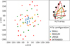 |
Fig. 1 Coverage of the (u, v)-plane obtained from the VLTI/MATISSE observations of 3 Puppis. The legend in the lower-right corner indicates the colours corresponding to the four AT configurations used: small (blue), medium (orange), large (green), and extended (red). A schematic map of the VLTI baselines, using the same colour code, is shown in the upper-right corner. East corresponds to increasing x-axis values, and north to increasing y-axis values. |
2.3 Data processing
The MATISSE observations in the L-, M-, and N-bands were reduced using the standard MATISSE data reduction software (DRS) version 2.0.02 (Millour et al. 2016). This pipeline consists of recipes developed by the consortium in the ESO CPL-based reduction framework EsoRex (v3.13.5), plus a set of Python libraries mat_tools3. The pipelines produced five reduced and calibrated data files in the OIFits format (Duvert et al. 2017), which contain various interferometric quantities. However, for our analysis we focused on only two quantities that were needed for the image reconstruction procedure: the squared visibility (V2) and the closure phase (CP) observables. The final reduced and calibrated data for the five observations were then merged into a single file using the OiFitsExplorer tool by the Jean-Marie Mariotti center (JMMC)4. The final L-, M-, and N-band data are plotted as a function of spatial frequency, B/λ, in Fig. 2. The spatial frequency quantifies the number of interference fringe cycles that can be resolved by MATISSE within an angular separation of one milliarcsecond, hence the unit of cycles per milliarcsecond (cycles mas−1).
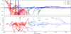 |
Fig. 2 VLTI/MATISSE squared visibility data, denoted V2, in logarithmic scale (top plot) and closure phase data, denoted CP, (bottom plot) of 3 Puppis in the L- (blue), M- (green), and N- (red) bands, plotted as a function of spatial frequency B/λ. The vertical dashed lines indicate the approximate positions of the first visibility nulls in the three bands with the same colour code. The horizontal dashed line marks the visibility plateau at long baselines in the L-band, which reflects the relative flux contribution from the unresolved central source. |
2.4 Qualitative analysis
From the V2 curves displayed in the top panel of Fig. 2, we can estimate the characteristic size of 3 Pup’s circumstellar disc by identifying the position of the first visibility null under the uniform disc approximation. In the L-band, the null occurs at approximately 0.07 cycles mas−1, corresponding to a size5 of about 14 mas. In the N-band, the first null indicates a larger characteristic size of approximately 33 mas. This clearly demonstrates the increasing extent of the CE from the L-band, which traces warm dust near the sublimation temperature, to the N-band, which is more sensitive to cooler material. The V2 plateau reached at the longest baselines in the L-band provides an estimate of the flux contribution from the compact central source, accounting for approximately 10% of the total flux. In contrast, this plateau level cannot be accurately determined from the M-and N-bands data based on the V2 alone.
CP curves displayed in the bottom panel exhibit significant variations at spatial frequencies above 0.06 cycles mas−1 in the L- and M-bands, and above 0.04 cycles mas−1 in the N-band. Such variations are commonly observed in circumstellar discs and are typically attributed to the asymmetric (or skewed) aspect of the inner rim of the dusty disc (Monnier et al. 2005; Lazareff et al. 2017). However, this effect alone cannot account for the non-zero CPs observed in both L- and M-bands at spatial frequencies lower than those probing the inner rim. Based on estimates from Table 1, the inner rim lies at a radius of around 5.7 mas, corresponding to a spatial frequency of approximately 0.08 cycles mas−1. We observe a CP signal of approximately ±20° over the spatial frequency range 0.02-0.05 cycles mas−1 in the L- and M-bands. It clearly indicates asymmetries located at higher spatial scales - around 20 to 50 mas - that are well beyond the expected position of the inner rim. Similarly, the CP variations observed in the N-band between 0.025 and 0.05 cycles mas−1 are difficult to reconcile without invoking large-scale asymmetries within the disc structure. Finally, we note that, similarly to the VLTI/MIDI data of 3 Pup analysed by Meilland et al. (2010), a clear broad silicate emission feature is present in the N-band, leading to a visibility drop around 10 μm and resulting in a U-shaped visibility variation across the band for each partially resolved baseline.
3 Image reconstructions
The (u, v)-plane coverage obtained from our observations is dense and spatially well distributed (see Fig. 1), making these MATISSE interferometric observables suitable for the use of image reconstruction techniques (Thiébaut 2009). In this section, we applied two different algorithms to reconstruct images from the MATISSE data across all MATISSE spectral channels. First, we performed a statistical analysis of the images reconstructed with the MiRA software, along with PYRA and MYTHRA which are two new Python-based interfaces for MiRA (Drevon et al. in prep.). The different steps of this statistical framework are outlined in Sect. 3.1. Then, we used the SPARCO algorithm, specifically developed for reconstructing images of CEs (see Sect. 3.2), to compare with the images obtained with MiRA (see Sect. 3.3). Both methods offer complementary advantages: MYTHRA enables the production of statistically robust images, while SPARCO enhances image contrast by subtracting the contribution of a bright central source.
3.1 Statistical image reconstruction procedure
3.1.1 MiRA imaging tool
The multi-aperture image reconstruction algorithm (MiRA; Thiébaut 2008) is a software based on a Bayesian approach that integrates regularisation functions to effectively reconstruct high resolution images from sparse interferometric data, even under challenging conditions such as limited Fourier phase information. As explained exhaustively by Le Besnerais et al. (2008) and Thiébaut (2008), the algorithm follows a gradient-descent method search to minimise the total chi-squared function  (also known as the cost or penalty function), defined as
 (1)
(1)
where fdata denotes the data fidelity term - measured using the chi-squared statistics6 -, fprior the regularisation term, and μ a weighting scalar referred to as the hyperparameter that controls the trade-off between them. After testing multiple reconstructions, the hyperbolic regularisation, an edge-preserving smoothness prior, was found to be the most suitable regularisation function as it outperforms the quadratic criterion, especially for extended objects with sharp features (e.g. disc edge such as an inner rim), while quadratic regularisation tends to over-smooth the edges of structures detected within the 3 Pup system.
Eq. (2) shows how the hyperbolic regularisation,  , is implemented in MiRA. This prior function relies on two tunable parameters: the scale parameter, s, and the edge-gradient threshold parameter, τ, which estimates the typical absolute difference between neighbouring pixels.
 (2)
(2)
 (3)
(3)
with x the sought object distribution (i.e. the reconstructed image of the science target), p and q the pixel indexes used to navigate through the dimensions of the sought two-dimension image, and C the cost function. Finally, MiRA requires an initial image as a starting point for the iterative reconstruction process. This initialisation can be either a simple parametric model (e.g. uniform disc, limb darkened disc, Gaussian disc) fitted to the data beforehand, or a centred point source (i.e. Dirac delta function). We chose the latter approach as the starting image of each MiRA image to minimise prior assumptions about the object’s morphology.
3.1.2 Image grid synthesised with PYRA
The IR images were reconstructed using PYRA7, a Python userfriendly wrapper designed to efficiently generate thousands of image reconstructions, enabling extensive exploration of MiRA’s free parameter space. A step-by-step summary of the reconstruction procedure follows.
Step 1: image characteristics. The field of view (FoV) and pixel size of the reconstructed images were determined based on the (u, v)-plane coverage (see Fig. 1). From this coverage, two key quantities were extracted: Bmax and Bmin, corresponding respectively to the longest and the shortest projected baselines used for the observation of 3 Pup; see Table A.1 for the values. The pixel size was estimated using the lowest angular size resolved by MATISSE during 3 Pup observations, noted θr, at a given wavelength8 λ0, and was defined as
 (4)
(4)
However, due to the sampling criterion, the pixel size of the resulting synthetic image should be equal to θ+, set to half the smallest angular resolution of the instrument (Thiébaut 2009). The physical FoV of the reconstructed image was ultimately determined by the interferometric FoV, instead of the photometric FoV, which following Tazzari et al. (2018) is given by
 (5)
(5)
Step 2: parameters sampling. To ensure that PYRA probed efficiently both the FoV and the pixel size parameter spaces, seven different FoV values (= NFoVgrid) and four different pixel size (= Nscalegrid) values were randomly taken from the following intervals
![Mathematical equation: \mathrm{FoV}_\mathrm{grid} &=& \overbrace{[0.5 \times\,\mathrm{FoV}_\mathrm{interf}\,,\ldots\,, 1.5\times\,\mathrm{FoV}_\mathrm{interf}]}^\text{7 values} ,\\](/articles/aa/full_html/2025/12/aa56615-25/aa56615-25-eq15.png) (6)
(6)
![Mathematical equation: \theta_\mathrm{grid} &=& \underbrace{[\theta^+\,,\ldots\,, \theta_\mathrm{r}]}_\text{4 values}\,\,](/articles/aa/full_html/2025/12/aa56615-25/aa56615-25-eq16.png) (7)
(7)
Table B.1 informs of the values obtained for the angular resolution of MATISSE and the physical FoV for each spectral band covered. Then, for each combination of FoV and pixel size values, we established a grid of values for the regularisa-tion parameter of the hyperbolic prior function (τgrid). Since τ depends on both pixel size and FoV quantities (see Eq. (8)), the grid was reinitialised whenever either variable changes within a given spectral band. As a result, the threshold parameter was systematically adapted to the spatial characteristics of the reconstructed image. The six values of τ (= Nτgrid) were chosen logarithmically spaced and computed as
![Mathematical equation: \forall (k,l) \in [\![1,4]\!] \times [\![1,7]\!],\, \tau^{k,l} = \left(\frac{\theta_\mathrm{grid}^k}{\mathrm{FoV}_\mathrm{grid}^l}\right)^2\label{eq:tau} \\](/articles/aa/full_html/2025/12/aa56615-25/aa56615-25-eq17.png) (8)
(8)
![Mathematical equation: \mathrm{hence} \quad \tau_\mathrm{grid}^{k,l} = \overbrace{\left[\frac{\tau^{k,l}}{10^4}\,,\frac{\tau^{k,l}}{10^3}\,, \frac{\tau^{k,l}}{10^2}\,, \frac{\tau^{k,l}}{10}\,, \tau^{k,l}\,, 10\times\tau^{k,l} \right]}^\text{6 values}\,.](/articles/aa/full_html/2025/12/aa56615-25/aa56615-25-eq18.png) (9)
(9)
The index k refers to the kth component of the pixel scale grid (θgrid; see Eq. (7)), while l denotes the lth component of the FoV grid (FoVgrid ; see Eq. (6)), both defined for each spectral band.
Step 3: hyperparameter. To identify the optimal hyperparameter value and produce the best possible reconstructed image, we performed a broad logarithmic search with PYRA across the interval [100, 108]. The sampling strategy of the hyperparameter grid consisted of generating randomly twenty values of μ (= Nμgrid), gathered under the denoted μgrid, within the mentioned interval. However, these μ values were reinitialised for every τ value explored in  (see Eq. (9)), ensuring that each τ uses a new sampling of μgrid, leading to a comprehensive exploration of the hyperparameter space rather than a fixed linear grid and preventing also redundant sampling. In other words, for every τ value, we explored a full different set of Nμgrid values of μ.
Step 4: iteration threshold. The remaining MiRA variables were kept at their default values in PYRA: scale of finite differences η = 1, tolerance factors ftol = gtol = xtol = 0, and total flux normalisation ftot = 1. The maximum number of iterations (or evaluations) was set to 1000. Drevon et al. in prep. reported that this value constitutes a reasonable limit for achieving convergence in MiRA to a low χ2 image while minimising artefacts.
Step 5: grid synthesis. With all the aforementioned variables set, PYRA was run by systematically exploring a grid of each combination of μ, τ, FoV and pixel size values. For each spectral band sought, it resulted in a grid of images9 with a total of NMiRAgrid = 3360 different reconstructed images10.
3.1.3 Averaged images computed with mythra
Once PYRA generated the grid of synthetic images, MYTHRA11 was used to derive a final image for each spectral band. To do so, MYTHRA analysed the PYRA grid by identifying the optimal hyperparameter value, denoted μ+, based on an L-curve diagram.
By definition an L-curve plots the resulting chi-squared (χ2) value of each synthetic image in the PYRA grid as a function of its associated hyperparameter value. This graphical representation helps determine the μ+ value because it corresponds to the inflection point of this curve. This point is located just before χ2 begins to diverge to a plateau (Dalla Vedova et al. 2017) and MYTHRA estimated it using a gradient-based search. As μ increases, the influence of the data in the minimisation process decreases, leading to an increase in χ2. The set μ+ value therefore marks the transition at which the regularisation term begins to dominate and degrade the model’s fit to the data.
The L-curves obtained in the L-, M-, and N-bands for 3 Pup MATISSE data, along with their corresponding μ+ values, are shown in Fig. B.1. Then MYTHRA established a robust subset of the PYRA grid by keeping only the reconstructed images in the vicinity of the inflection point to exclude outliers. The χ2 criterion was also employed to refine the selection of the final subset by constraining the vertical axis of the L-curve plot. After the identification of a statistically reliable subset of reconstructed images (i.e. combining the μ+ and χ2 criteria), MYTHRA resampled all the selected images to a common pixel size and spatial resolution - the rest of MiRA variables were kept identical otherwise.
Before producing the final averaged image, MYTHRA applied an outlier rejection step to refine one last time the subset. This was done through an iterative process in which images were added one by one to a cumulative mean. Therefore, at each iteration, if the inclusion of a new image caused the global χ2 to exceed a predefined threshold (χglobal = 10; in this work), the current image was then excluded from the final subset. The resulting ‘cleaned’ subset was used to eventually compute the final averaged image.
The final averaged images (one for each spectral band studied) are shown in the first row of Fig. 4 and are called the ‘MYTHRA images’. The corresponding (simulated) V2 and CPs extracted from the averaged image, shown in Fig. 3, indicate a satisfactory fit to the MATISSE data given the complexity of the datasets, with global χ2 values equal to 7.6, 5.6, and 2.2 for the L-, M-, and N-bands respectively. Table B.2 summarises the MYTHRA statistics obtained at each step to produce the averaged images.
3.2 SPARCO imaging tool
The combination of MiRA with the PYRA and MYTHRA interfaces enables the reconstruction of statistically relevant images. However, in the context of CEs, the dynamic range of a reconstructed image can be significantly limited by the presence of a bright, central point-like source (i.e. the unresolved component) - in our work, it refers to the combined emission from the binary system and the gaseous disc. To address this limitation, we complemented our imaging analysis with the semi-parametric approach for reconstruction of chromatic objects (SPARCO; Kluska et al. 2014), an algorithm specifically designed to overcome such challenges.
In SPARCO, the optical interferometric data were modelled as the sum of a geometrical model (generally a chromatic unresolved object) plus a reconstructed image, each with their own spectrum. Within this framework, the image was reconstructed using the MiRA algorithm (along with its specific parameters), while the model component was described using additional parameters. We used the implementation of the SPARCO algorithm in the 0Imaging service12 by the JMMC which provides user-friendly access to several interferometric image reconstruction algorithms. The ‘SPARCO images’ presented in the bottom row of Fig. 4 were reconstructed separately over the L-, M-, and N-bands, and with the following set parameters: a reference wavelength set at 3.0 μm; a black-body profile with a temperature of 1500 K for the MIRA image initialised with a centred Gaussian disc; and a point-source object with a flux ratio 0.12 (except for the M-band which is equal to 0.15) and a temperature of 10 000 K for the geometric model.
3.3 Comparison between MYTHRA and SPARCO images
To enable a direct comparison between SPARCO and MYTHRA images in each spectral band of MATISSE, we applied the point spread function (PSF) subtraction technique on the MYTHRA reconstructions. The technique began with the averaged image produced by MYTHRA (see Sect. 3.1.3). From this unconvolved image we subtracted a Gaussian PSF centred on the brightest pixel and scaled to match its maximum intensity. The full width at half maximum (FWHM) of the PSF was equal to θr as defined in Eq. (4) (see the values for each band in Table B.1). The residual image was then convolved with the interferometric beam characterised in Table A.4. The resulting image from this operation was denoted as the ‘MYTHRA-PSF’ image and is shown in the second row of Fig. 4. For consistency, the same procedure was also applied to the VLTI/AMBER K-band image from Millour et al. (2011), which is also displayed in the same figure.
The L-band images reconstructed with the imaging tools MYTHRA and SPARCO are in excellent agreement, both revealing a skewed inner rim with the same orientation of asymmetry and similar contrast. In addition, an elongated feature located approximately 20 mas south-east of the central object is clearly visible in both reconstructions - hereafter referred to as the southeastern (SE) elongated clump. This structure is also present in the M-band images, although with lower contrast.
Additionally, a second structure seems to appear in the northwest (NW) region of M-band images, especially for SPARCO and MYTHRA-PSF. Both exhibit a skewed inner rim. However, in the case of the SPARCO image the orientation of the skewness is reversed, which is unlikely to reflect a physical property of the system. The N-band images likewise suggest the presence of the eastern structure and a fainter one to the west. While the overall sizes are comparable, SPARCO images appear smoother, with fewer artefacts, than those produced by MYTHRA.
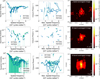 |
Fig. 3 Comparison between the interferometric observables extracted from the MYTHRA averaged images (in blue) and the VLTI/MATISSE data of 3 Puppis (in green), shown respectively in the L-band (first row ), in the M-band ( second row ), and in the N-band ( third row ). Left column : squared visibility amplitudes as a function of spatial frequency in logarithmic scale. Central column : closure phases as a function of spatial frequency, computed using the longest baseline. Right column : final averaged images resulting from MYTHRA, normalised to unity (i.e. the sum over all pixels equals one), with a logarithmic colour scaling, and not convolved with the interferometric beam. The minimum value for each brightness scaling is set to half the standard deviation of the associated image to filter out the artefact produced by the MiRA algorithm. |
4 Discussion
4.1 Large-scale asymmetries detected in the disc
The reconstructed images allowed us to identify the main spatial components of 3 Pup’s CE and thereby characterise the general morphology of its dusty disc across different mid-IR spectral bands. Thanks to the statistical image reconstruction procedure presented in Sect. 3.1, the final images plotted in Fig. 4 revealed a large-scale brightness distribution asymmetry in the SE region of the CE in the L-band (see Sect. 3.3). This asymmetry, which we refer to as an elongated clump, seems to be responsible for the non-zero CP signal at small spatial frequencies in the MATISSE data (i.e. around 0.02-0.05 cycles mas−1 ), as displayed in the bottom panel of Fig. 2.
Therefore, our findings demonstrate that the CE of 3 Pup cannot be described by a simple disc with a skewed inner rim alone since at least one bright asymmetric structure is consistently detected in all IR images, at approximately 20 mas SE of the image centre - position marked by the blue cross in Fig. 4 and as determined in Sect. 4.2. The presence of this elongated clump is also detected in the M- and N-bands images as it appears at a similar SE location from the image centre. Moreover, another (fainter) asymmetry in the NW region seems to be visible in the M- and N-bands images but is absent from the L-band image.
4.2 Geometric modelling of the L-band asymmetry
To constrain quantitatively the position of the asymmetric feature identified in the L-band images as the SE elongated clump, we used oimodeler13 (Meilland et al. 2024), a modular modelling tool for optical interferometry which includes a Markov chain Monte Carlo sampling algorithm (emcee; Foreman-Mackey et al. 2013). The fit was performed in the L-band only and was limited to low spatial frequencies (i.e. baselines shorter than 40 m) to minimise contamination from smaller-scale structures. The central object was modelled as a centred Gaussian, while the asymmetry was modelled as a second Gaussian component. The fit yields a position of the asymmetry at x = 14.21 ± 0.03 mas and y = -8.79 ± 0.04 mas, or a separation with the central source of Rref = 16.71 ± 0.03 mas with a 121.7° orientation from the north to the east (also known as the position angle and denoted PA).
Such values are consistent with the early qualitative analysis made in Sect. 2.4 and the observations made in Sect. 3.3 based on the reconstructed images shown in Fig. 4 where this fitted SE asymmetry position is indicated by a blue cross. Converting this angular separation Rref to physical units, we obtain a projected physical distance of approximately Rref = 16.71 ∙ 10−3 × 631 ~ 10 au from the 3 Pup system centre at the adopted distance dGeDR2 (Rref ~ 17 au at dPGeDR3 respectively).
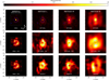 |
Fig. 4 Final image reconstructions of 3 Puppis in the mid-infrared using MiRA, MYTHRA, and SPARCO imaging tools. The FoV for each image is (60 mas × 60 mas) with north up and east left. The dashed blue ellipse indicates the best-fit inner rim of the dusty disc derived from VLTI/AMBER data, while the blue cross marks the SE elongated clump best-fit position, denoted Rref, from MATISSE L-band geometric modelling (at a distance of 16.71 ± 0.03 mas from the image centre). Brightness colour scale is normalised to peak intensity (i.e. maximum pixel value). K-band image : the left-most column shows the images obtained with VLTI/AMBER data by Millour et al. (2011). In the first row the median MiRA image is displayed, and the last two rows present the identical convolved median MiRA image with the λ/2 B max PSF subtraction applied. L-M-N-bands images : the remaining three columns display the images obtained with VLTI/MATISSE. On the first row the resulting MYTHRA averaged image is shown. The second row shows the convolved image of MYTHRA with the λ/2Bmax PSF subtraction applied. The last row gives the resulting SPARCO image, convolved with the interferometric beam. |
4.3 Comparison to previously published VLTI data
4.3.1 VLTI/AMBER K-band data
The 3 Pup system was previously observed in the near-IR during the first semester of 2010 using the VLTI/AMBER instrument. The observations were carried out at high spectral resolution (R~ 12000), centred on the prominent Brγ emission line. The data, published in Millour et al. (2011), allowed the authors to constrain the geometry of the object in the near-IR continuum - revealing a compact source surrounded by a skewed inner rim of the dusty disc - but also the geometry and dynamics of the inner gaseous disc, which was found to be dominated by Keplerian rotation. The image reconstruction of the K-band data was performed using MiRA and a self-calibration algorithm, producing narrow-band images across the Brγ line and the adjacent continuum.
The data were modelled using a skewed ring to represent the inner rim of the dusty disc, along with a kinematic model for the line-emitting gas. They found a diameter of 13.9 mas for the dusty inner rim and an elongation ratio (also known as flattening) of 1.27, which corresponds to an inclination angle of 38° under the assumption of a geometrically thin disc. These estimates are consistent with the first null at 0.07 cycles mas−1 qualitatively estimated in Sect. 2.4. The K-band median AMBER image, along with its PSF-subtracted version, are displayed in the left column of Fig. 4. The best-fit inner rim model from Millour et al. (2011) is overplotted over the reconstructed K-, L-, M-, and N-band images. The size, flattening, PA, and skewness of the dusty inner rim derived from the AMBER data (see Table 1) are fully consistent with our MATISSE reconstructions in the L- and M-bands, shown in the same figure.
However, we note that the bright SE elongated clump observed in the MATISSE images as detailed in the previous Sects. 4.1 and 4.2 is not present in the AMBER data. This discrepancy may be due to the limited FoV used for the AMBER image reconstruction, which was restricted to 32 mas, while in the L-band MATISSE image instead was reconstructed with a FoV equal to 63 mas.
4.3.2 VLTI/MIDI N-band data
The 3 Pup system was also observed in the N-band with the VLTI/MIDI instrument by Meilland et al. (2010) between October 2006 and January 2008. The authors acquired data on nine baselines ranging from 13 to 71 m, and determined the wavelength-dependent extension of the CE by fitting a two-component model consisting of an elliptical Gaussian distribution and an extended background. To enable a direct comparison between the MIDI and MATISSE datasets, since they both observed in the N-band, we restricted the analysis to V2 data only, as CPs were excluded because MIDI was a two-telescope beam-combiner instrument at the VLTI (Leinert et al. 2003). By comparing the V2 data from MATISSE to MIDI, we find that they are in qualitative agreement as shown in Fig. C.1.
For a quantitative comparison between the MIDI and MATISSE datasets, we kept from the MATISSE V2 data only measurements with baselines shorter than 70 m to be consistent. Then, we fitted the same chromatic two-component geometric model, consisting of an elongated Gaussian disc distribution and a fully unresolved component (i.e. point source function), to each dataset independently using oimodeler. Two physical parameters were set as chromatic quantities: the major-axis FWHM of the Gaussian distribution’s major axis and the elongation ratio of the disc. The chromatic plot of these derived quantities is shown in Fig. 5.
We note that while the FWHM values are consistent in the 9.2-12 μm wavelength range (ranging from 28 to 30 mas) for both instruments, a significant discrepancy is observed at shorter wavelengths. Specifically, the MIDI data show a drop in the FWHM to 16 mas at 8 μm, whereas the MATISSE data yield a larger value of 23 mas. Another key difference lies in the elongation ratio, which is systematically higher for MIDI (average of 1.54) than for MATISSE (average of 1.23), and follows a different trend as a function of wavelength. A possible explanation for the reduced flattening is the effect of the asymmetries, which tend to artificially enhance the east-west expansion of the disc in the N-band, as seen in the reconstructed images in Fig. 4.
Concerning the remaining quantities of the Gaussian component of the geometric model fitting that were assumed achromatic, we obtain for the MIDI data a PA of +22 ± 59° and a relative flux of 77 ± 3%, while for the MATISSE data we find a PA of -14 ± 1° and a relative flux of 83 ± 1%. Table C.1 summarises the values derived for fitted parameters of the chromatic geometric model.
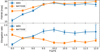 |
Fig. 5 Spectral evolution of the fitted disc parameters from a chromatic two-component geometric model applied to 3 Puppis N-band observations obtained with the VLTI/MIDI (in blue) and VLTI/MATISSE (in orange) instruments. Top plot : the FWHM of the major-axis as a function of wavelength. Bottom plot : elongation (or flattening) ratio as a function of wavelength. |
4.3.3 Radiative transfer model with MC3D
Moreover, the authors of Meilland et al. (2010) also compared the MIDI data to radiative transfer models computed for instance with the MC3D code (Wolf et al. 1999; Wolf 2003). Although their model was fitted using sparse data with significantly shorter baselines and no CP information, we decided to compare the MATISSE N-band data to synthetic V2 and CPs generated from their best-fit Keplerian-disc model (referred to as the MC3D model). As shown in Fig. C.2 with the synthetic interferometric observables displayed in red, this model poorly reproduces the MATISSE data, yielding a reduced χ2 of 117.
While the Keplerian-disc model qualitatively fits the overall size and flattening of 3 Pup MATISSE data in the N-band, it fails to reproduce the asymmetries associated with the non-zero CP signal. However, the inability to fit the CPs at frequencies below those of the inner rim is expected, as previously mentioned in Sect. 2.4. We tried to minimise the reduced χ2 value by adding to the original MC3D model an elongated Gaussian component (i.e. {MC3D + EG} model) to account for the SE asymmetry revealed in MATISSE data (see Sect. 4.1). This second model fitting led to an improved χ2 value of 47.
Thanks to this successful attempt, we tried also to add a second elongated Gaussian component, defined as the {MC3D + 2EG} composite model, to account for the fainter NW asymmetry visible in the M- and N-band images. Finally we obtain an even better agreement than the two previous models, with a reduced χ2 value equal to 24, and achieve a qualitative fit of the CP signature at short spatial frequencies as shown overplotted on the same Fig. C.2, in blue. The best-fit parameter values for the two elliptical Gaussians of the {MC3D + 2EG} model are given in Table 2 and the corresponding image of the composite model is shown in Fig. 6. From the fitted Cartesian coordinates, we compute for each elliptical Gaussian component the radius, R, from the image centre. We obtain RSE = 18.1 ± 1.8 mas and RNW = 19.0 ± 2.3 mas for the SE and NW components respectively. The best-fit position of the brighter asymmetry (i.e. SE elongated clump) is consistent with the values derived in Sect. 4.2, and the latter contributes to about 13% of the total flux at 10 μm.
Best-fit parameters for the two elliptical Gaussian disc components from the {MC3D + 2EG} model.
4.4 Possible origins for the asymmetric structures
The origin of the asymmetries observed in the mid-IR images of 3 Pup remains uncertain. However, 3 Pup is a confirmed binary system composed of two evolved stars: a SG primary and a dwarf companion, separated by 1.11 au, with estimated masses of 8.8 ± 0.5 M⊙ and 0.75 ± 0.25 M⊙ respectively, as recalled in Table 1. Miroshnichenko et al. (2020) propose that the circumbi-nary disc likely formed as a result of common binary evolution involving mass transfer between the components, with part of the transferred material being ejected into the circumstellar environment. We consider four main hypotheses (Hyps.) to explain the observed elongated structures SE and NW as defined in Sect. 4.1.
Hypothesis 1: direct mass ejection. The asymmetric structures could correspond to over-densities in the circumbinary disc, generated by gravitational interactions between the companion and the disc itself. Such interactions lead to direct mass transfer through the Lagrangian points L2 and L3. In this scenario, material ejected from the inner binary system would create co-rotating structures with close to Keplerian velocities at the disc location where the elongated clumps are observed.
Hypothesis 2: precessing spiral density waves. Alternatively, the elongated structures similar to spiral-like features, might arise from spiral density waves generated by gravitational interactions between the dwarf and the disc material. These waves form at Lindblad resonances (i.e. where the companion’s gravitational influence disturbs the disc material) and propagate through the gas and dust (Cuello et al. 2025). This scenario has been tested numerically and, for example, has proposed to explain the symmetric spiral structures observed in the VLT/SPHERE images of the young stellar object HD 100453 (Benisty et al. 2017). Unlike co-rotating structures, spiral density waves would precess at much lower velocities.
Hypothesis 3: influence of a third stellar component. The asymmetries could also result from the gravitational influence of a putative third stellar companion, located several au from the central binary system. This could manifest either as a locally formed gravitationally bound object (e.g. giant planet, brown dwarf) embedded within the disc material at the observed location, or as density enhancements in the circumstellar material caused by gravitational perturbations from a more distant third companion.
Long-term IR monitoring of the disc can help discriminate between the three scenarios. Assuming that the large-scale asymmetric structures, especially the SE one, follow a quasi-Keplerian orbit at the estimated distance Rref ~ 10 au (see Sect. 4.2), it would imply an orbital period of roughly 11 years. Comparison of future reconstructed images with new MATISSE observations acquired over a time span of 4-5 years (which corresponds to ~40% of the SE structure probable orbital period) with the results reported here would clearly indicate whether the structure has moved in a Keplerian orbit (supporting Hyps. 1 and 3) or has remained at the same position (strengthening Hyp. 2). If none of these scenarios are favoured by future observations, a fourth one should be considered.
Hypothesis 4: radiative transfer effects. The asymmetries could arise from a combination of radiative transfer effects (e.g. opacity, scattering) and the particular geometry of the circumstellar environment illuminated by the central binary. This last hypothesis would be strengthened if new IR images taken several years later show the same asymmetric structures at identical positions and with similar brightness distributions.
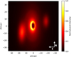 |
Fig. 6 Best-fit image at 10 μm using the N-band MATISSE data of 3 Puppis. The fit is performed combining MC3D code with two elliptical Gaussian disc models ({MC3D + 2EG} model) to describe the asymmetries revealed by MYTHRA and SPARCO image reconstructions. The model fitting results in a reduced chi-squared value of 24. East corresponds to increasing x-axis values, and north to increasing y-axis values. |
4.5 Physical constraints on the disc of 3 Puppis
Thanks to the MATISSE observations, our study demonstrates that the asymmetric structures detected in the dusty circumbi-nary disc of 3 Pup are robust across different imaging methods and coherent over three mid-IR spectral channels. The confirmed presence of these asymmetries raises a fundamental astrophysical question, namely, whether they are driven by local disc instabilities, such as gravitational fragmentation or massive embedded bodies, or whether they reflect global tidal perturbations from the central binary. To discriminate between the scenarios proposed in Sect. 4.4, we performed a hydrodynamic (HD) study to assess the physical plausibility of each scenario. While a detailed radiative transfer study would provide more definitive constraints, this preliminary assessment enables us to evaluate competing scenarios and improve our understanding of the physical mechanisms underlying the observed structures.
4.5.1 Hydrodynamical analysis
The HD analysis of the SE elongated clump provides critical constraints on the physical mechanisms responsible for the observed asymmetries. Our calculations yield a gas mass estimate of Mclump ≃ 3.73 × 10⁻² M⊙ (see Appendix D.2.4) and demonstrate extreme gravitational stability at the reference radius Rref, with Toomre parameter values Qref ≫ 104 (see Appendix D.2.1). These values exceed the classical threshold for axisymmetric gravitational instability (Q < 1.5; Durisen et al. 2007) by more than four orders of magnitude, effectively ruling out local gravitational collapse processes such as disc clumping due to self-gravity and fragmentation at the inner rim region (Kratter & Lodato 2016).
The mass budget analysis further constrains the nature of the observed structure. Even under optimistic assumptions regarding the gas-to-dust ratio (δ = 104; representing a 100-fold increase from our baseline estimate), the clump mass remains insufficient for gravitational binding (~0.2 MJup). This mass falls two to three orders of magnitude below the typical threshold required to form a bound object with a circumplanetary disc (Zhu et al. 2015). This analysis strongly disfavours direct mass ejection leading to gravitational clumping (i.e. Hyp. 1) and makes the presence of embedded giant planets or brown dwarfs at Rref highly unlikely (i.e. Hyp. 3). Any such body would require a formation history independent of local gravitational collapse, such as external capture or core accretion from an earlier evolutionary epoch. On the other hand, the viscosity evolution analysis reveals timescales at the clump’s position of 9.75 × 10⁴ yrs that exceed both the central binary orbital period and the estimated period for structures at Rref by more than two orders of magnitude. Consequently, any asymmetry observed around the dusty inner rim is unlikely to originate from viscous redistribution of mass, given the long viscous timescales relative to the relevant orbital periods, thereby supporting the persistence of coherent spiral structures.
Collectively, these results strongly favour Hyp. 2, meaning that the observed asymmetries are best interpreted as tidally induced spiral density waves generated by gravitational interactions between the central binary and the circumbinary disc, as described by Artymowicz & Lubow (1996) and Poblete et al. (2019). This interpretation is consistent with similar structures observed in other binary systems and young stellar objects (Benisty et al. 2017). Detailed calculations characterising the physical properties of the circumbinary disc, including gravitational stability criteria, viscous evolution timescales, and mass distribution analysis, are presented in Appendix D.2. The relevant physical equations and numerical parameters are summarised in Tables D.1 and D.2.
4.5.2 Hydrodynamical simulation of the asymmetries
To assess whether the SE and NW asymmetries detected in the circumbinary disc of 3 Pup could originate from a tidally excited spiral density wave, we constructed a two-dimensional analytic model of the disc’s surface density field Σ(R,φ) (see formula in Appendix D.3). This model assumes a Keplerian disc structure with a background surface density profile following Σ0(R) ∝ R−3/2, consistent with steady-state viscous evolution (Lynden-Bell & Pringle 1974). The reference point is set to the SE clump position in polar coordinates: R0 = Rref ≃ 16.71 mas and φ0 = tan−1(y/x)ref = -31.74° (derived from the L-band geometric modelling in Sect. 4.2). Superimposed on the surface background, we implemented a trailing logarithmic spiral characterised by the pitch angle ψ. This logarithmic formulation is widely adopted in analytical and numerical studies of tidally excited spirals (e.g. Ogilvie & Lubow 2002; Rafikov 2002; Dong et al. 2015), as it naturally captures the characteristic curvature and trailing structure of density waves launched at Lindblad resonances. Drawing from the HD simulations of Dong et al. (2015) and Zhu et al. (2015) who studied tidally perturbed discs around binaries with small mass ratios (i.e. Mc/M* ≪ 1) and with an aspect ratio ε ~ 0.05, we adopted the following model parameters input values: density contrast amplitude Γ = 0.2 (see justification in Appendix D.1), Gaussian angular width σφ = 20° (yielding an effective spiral Gaussian angular thickness of  ), and ψ = 15° .To generate similar observational conditions, we projected the vertical optical depth onto the sky plane, assuming axisymmetric thermal emission at a constant temperature (see justifications in Appendix D.1), to mimic mid-IR radiative transfer. The resulting synthetic surface density distribution of 3 Pup’s disc with simulated tidal perturbations is presented in Fig. D.1, while Fig. 7 shows the direct overlay of the spiral density model with the N-band reconstructed MYTHRA image (original image plotted at the bottom right panel of Fig. 3). The simulated spirals exhibit a trailing orientation confined within a ~15 au radius, successfully reproducing the elongated clumps in the SE and NW regions of 3 Pup’s disc in both N-band MYTHRA and SPARCO images (see Fig. 4). Importantly, this reproduction requires neither a third companion nor gravitational instability and is fully consistent with the long viscous timescales derived in Sect. D.2.3. The moderate surface density enhancement (i.e. Γ ~ 20%) remains consistent with the dynamical stability conditions derived in Sect. D.2.1 (i.e. Q ≫ 1 ensuring that the disc remains gravitationally stable in the perturbed region). This modelling demonstrates that the observed asymmetries can arise from a tidal response of the circumbinary disc to the inner binary’s gravitational potential. The excellent agreement between our analytic spiral morphology and the N-band reconstructed images strongly supports the interpretation of tidally induced spiral waves. This scenario is dynamically stable, hydrodynamically plausible, and consistent with all available observational and theoretical constraints.
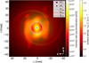 |
Fig. 7 Composite image showing the analytic spiral model superimposed on the reconstructed N-band MYTHRA image of 3 Puppis. The logarithmic colour scale represents the observed intensity of the N-band image (normalised to unity and expressed in ADU), while the spiral model is overlaid as a semi-transparent structure representing the local gas surface density normalised to 20% contrast. The red dashed circle marks the inner dust rim (Rrim ≃ 5.7 mas), and the black dotted circle indicates the radius of the SE asymmetric structure (Rref ≃ 16.71 mas) inferred from the L-band MYTHRA image. The curvature and radial extent of the two logarithmic spiral arms closely match the two asymmetries observed in the N-band image, located in the SE and NW regions of the dusty disc. |
5 Conclusion
We present new interferometric observations of the 3 Pup system with MATISSE in the L-, M-, and N-bands. The data were analysed for each spectral band using image reconstruction techniques including MYTHRA, a novel statistical framework to produce robust images, and the SPARCO algorithm.
Our analysis constrains the morphology of the dusty inner rim, revealing that its extent, flattening, and skewness are consistent with previous K-band results from AMBER. Comparison with earlier MIDI observations shows good compatibility, though our MATISSE data provide significantly enhanced information thanks to improved sensitivity, broader spectral coverage, access to longer baselines, and four-telescope configuration enabling CP measurements and hence the detection of asymmetries within the CE. Unlike results from first-generation VLTI instruments, our MATISSE images reveal a far more complex circumstellar morphology around the binary system of 3 Pup. While the inner dusty disc structure remains consistent with previous findings, we detect a bright, extended structure towards the SE, located at a projected distance of approximately 10 au at 631 pc - roughly three times the dust inner rim radius. A fainter, asymmetric structure is also observed in the opposite direction (i.e. NW), approximately 180° from the main asymmetric structure revealed in L-band images in the SE region.
To explain the nature and origin of these mid-IR asymmetries, we formulate four scenarios: (1) precessing gravity waves in the circumbinary disc due to the inner companion; (2) corotating spirals created by direct mass transfer from the inner system through Lagrangian points; (3) over-density created by an unknown tertiary companion further in the circumbinary disc; (4) radiative transfer effects. Our HD analysis demonstrates extreme gravitational stability across the entire disc (Q ≫ 104), ruling out bound massive objects or local collapse due to long viscous timescales (~104-105 years) and insufficient gas mass (~10−4MJup). Instead, the elongated clumps are best explained by tidally induced spiral density waves from the central binary, supporting the hypothesis (2). The synthetic spiral morphology successfully reproduces the observed structures, strongly supporting this interpretation as dynamically stable and consistent with theoretical HD predictions for circumbinary disc dynamics. Therefore, the referred elongated structures can rather be identified as dusty spiral arcs.
Follow-up interferometric observations, as well as a reanalysis of the archival AMBER data and a dedicated radiative transfer modelling, will help discriminate between scenarios. Refining our understanding of this system may shed light on mass-loss processes in evolved binaries and demonstrate the importance of the binary nature of B[e] stars.
Acknowledgements
Part of this work was supported by the observations collected at the European Organisation for Astronomical Research in the Southern Hemisphere under ESO programme(s) 0104.D-0669(A), 0104.D-0015(B), 0104.D-0554(A), 112.25C5.003. MATISSE collaboration is a consortium composed of institutes in France (J.-L. Lagrange Laboratory, Université Côte d’Azur, Observatoire de la Côte d’Azur Observatory, CNRS), Germany (MPIA, MPIfR, and the University of Kiel), the Netherlands (NOVA and the University of Leiden), and Austria (the University of Vienna). MA, AM, ADS, and FM acknowledge the support of the French Agence Nationale de la Recherche (ANR), under grant MASSIF (ANR-21-CE31-0018-01, www.anr-massif.fr), without which this work would not have been possible. MA also acknowledges the partial supported by the Early-Career Scientific Visitor Programme at ESO Chile (laureate of the 2024 research grant, www.eso.org/sci/activities/santiago/visitors.html). JV is funded from the Hungarian NKFIH OTKA projects no. K-132406, and K-147380. This work was also supported by the NKFIH NKKP grant ADVANCED 149943. Project no.149943 has been implemented with the support provided by the Ministry of Culture and Innovation of Hungary from the National Research, Development and Innovation Fund, financed under the NKKP ADVANCED funding scheme. JV acknowledges support from the Fizeau exchange visitors programme. The research leading to these results has received funding from the European Union’s Horizon 2020 research and innovation programme under Grant Agreement 101004719 (ORP). PA acknowledges the funding support from the Hungarian NKFIH project No. K-147380. This research has made use of the Jean-Marie Mariotti Center (JMMC) - MOIO, in particular ASPRO2 (www.jmmc.fr/english/tools/proposal-preparation/aspro), OiFitsExplorer, OImaging, and AMHRA (https://amhra.oca.eu/AMHRA/index.htm). This work has made use of data from the European Space Agency (ESA) mission Gaia (www.cosmos.esa.int/gaia), processed by the Gaia Data Processing and Analysis Consortium (DPAC, www.cosmos.esa.int/web/gaia/dpac/consortium). Funding for the DPAC has been provided by national institutions, in particular the institutions participating in the Gaia Multilateral Agreement. The following services and facilities have also been used: the SIMBAD and VIZIER databases (CDS, Strasbourg, France) and the NASA’s Astrophysics data System.
References
- Aidelman, Y. J., Borges Fernandes, M., Cidale, L. S., et al. 2023, A&A, 678, A21 [NASA ADS] [CrossRef] [EDP Sciences] [Google Scholar]
- Allen, D. A., & Swings, J. P. 1976, A&A, 47, 293 [NASA ADS] [Google Scholar]
- Artymowicz, P., & Lubow, S. H. 1996, ApJ, 467, L77 [NASA ADS] [CrossRef] [Google Scholar]
- Baade, D., Rivinius, T., Pigulski, A., et al. 2016, A&A, 588, A56 [NASA ADS] [CrossRef] [EDP Sciences] [Google Scholar]
- Babusiaux, C., Fabricius, C., Khanna, S., et al. 2023, A&A, 674, A32 [NASA ADS] [CrossRef] [EDP Sciences] [Google Scholar]
- Bailer-Jones, C. A. L., Rybizki, J., Fouesneau, M., Demleitner, M., & Andrae, R. 2021, AJ, 161, 147 [Google Scholar]
- Benisty, M., Stolker, T., Pohl, A., et al. 2017, A&A, 597, A42 [NASA ADS] [CrossRef] [EDP Sciences] [Google Scholar]
- Brown, A. G. A., Vallenari, A., Prusti, T., et al. 2018, A&A, 616, A1 [NASA ADS] [CrossRef] [EDP Sciences] [Google Scholar]
- Bujarrabal, V., Alcolea, J., Van Winckel, H., et al. 2013, A&A, 557, A104 [NASA ADS] [CrossRef] [EDP Sciences] [Google Scholar]
- Chen, P.-S., Liu, J.-Y., & Shan, H.-G. 2021, PASJ, 73, 837 [Google Scholar]
- Chentsov, E. L., Klochkova, V. G., & Miroshnichenko, A. S. 2010, Astrophys. Bull., 65, 150 [CrossRef] [Google Scholar]
- Chiang, E. I., & Goldreich, P. 1997, ApJ, 490, 368 [Google Scholar]
- Cruzalèbes, P., Petrov, R. G., Robbe-Dubois, S., et al. 2019, MNRAS, 490, 3158 [Google Scholar]
- Cuello, N., Alaguero, A., & Poblete, P. P. 2025, Symmetry, 17, 344 [Google Scholar]
- D’Alessio, P., Canto, J., Calvet, N., & Lizano, S. 1998, ApJ, 500, 411 [CrossRef] [Google Scholar]
- Dalla Vedova, G., Millour, F., Domiciano de Souza, A., et al. 2017, A&A, 601, A118 [NASA ADS] [CrossRef] [EDP Sciences] [Google Scholar]
- Dong, R., Zhu, Z., Chiang, E., & Fung, J. 2015, ApJ, 809, L5 [Google Scholar]
- Draine, B. T. 2011, Physics of the Interstellar and Intergalactic Medium (Princeton, NJ: Princeton University Press) [Google Scholar]
- Dullemond, C. P., Dominik, C., & Natta, A. 2001, ApJ, 560, 957 [NASA ADS] [CrossRef] [Google Scholar]
- Durisen, R. H., Boss, A. P., Mayer, L., et al. 2007, Protostars and Planets V, 607 [Google Scholar]
- Duvert, G., Young, J., & Hummel, C. A. 2017, A&A, 597, A8 [NASA ADS] [CrossRef] [EDP Sciences] [Google Scholar]
- Ellerbroek, L. E., Benisty, M., Kraus, S., et al. 2015, A&A, 573, A77 [NASA ADS] [CrossRef] [EDP Sciences] [Google Scholar]
- Foreman-Mackey, D., Hogg, D. W., Lang, D., & Goodman, J. 2013, PASP, 125, 306 [Google Scholar]
- Gaia Collaboration (Vallenari, A., et al.) 2023, A&A, 674, A1 [NASA ADS] [CrossRef] [EDP Sciences] [Google Scholar]
- Hartmann, L. 1998, Cambridge Astrophysics Series, 32, Accretion Processes in Star Formation (Cambridge University Press) [Google Scholar]
- Hayashi, C. 1981, in IAU Symposium, 93, Fundamental Problems in the Theory of Stellar Evolution, eds. D. S. D. Q. Lamb & D. N. Schramm (Dordrecht: Reidel), 113 [Google Scholar]
- Kenyon, S. J., & Hartmann, L. 1987, ApJ, 323, 714 [Google Scholar]
- Kluska, J., Malbet, F., Berger, J. P., et al. 2014, A&A, 564, A80 [NASA ADS] [CrossRef] [EDP Sciences] [Google Scholar]
- Kluska, J., Van Winckel, H., Hill, C. A., et al. 2018, A&A, 616, A153 [NASA ADS] [CrossRef] [EDP Sciences] [Google Scholar]
- Kratter, K., & Lodato, G. 2016, ARA&A, 54, 271 [NASA ADS] [CrossRef] [Google Scholar]
- Kraus, M. 2016, Bol. Asoc. Argentina Astron. Plata Argentina, 58, 70 [Google Scholar]
- Kraus, M., Cidale, L. S., Arias, M. L., et al. 2016, A&A, 593, A112 [NASA ADS] [CrossRef] [EDP Sciences] [Google Scholar]
- Lamers, H. J. G., & Pauldrach, A. W. A. 1991, A&A, 244, L5 [NASA ADS] [Google Scholar]
- Lamers, H. J. G. L. M., Zickgraf, F.-J., de Winter, D., Houziaux, L., & Zorec, J. 1998, A&A, 340, 117 [NASA ADS] [Google Scholar]
- Lazareff, B., Berger, J. P., Kluska, J., et al. 2017, A&A, 599, A85 [NASA ADS] [CrossRef] [EDP Sciences] [Google Scholar]
- Le Besnerais, G., Lacour, S., Mugnier, L. M., et al. 2008, IEEE J. Selected Top. Signal Process., 2, 767 [Google Scholar]
- Leinert, C., Graser, U., Przygodda, F., et al. 2003, Astrophys. Space Sci., 286, 73 [NASA ADS] [CrossRef] [Google Scholar]
- Liimets, T., Kraus, M., Moiseev, A., et al. 2022, Galaxies, 10 [Google Scholar]
- Lopez, B., Lagarde, S., Petrov, R. G., et al. 2022, A&A, 659, A192 [NASA ADS] [CrossRef] [EDP Sciences] [Google Scholar]
- Lynden-Bell, D., & Pringle, J. E. 1974, MNRAS, 168, 603 [Google Scholar]
- Meilland, A., Kanaan, S., Borges Fernandes, M., et al. 2010, A&A, 512, A73 [NASA ADS] [CrossRef] [EDP Sciences] [Google Scholar]
- Meilland, A., Scheuck, M., Varga, J., Matter, A., & Millour, F. 2024, SPIE Conf. Ser., 13095, 130952W [Google Scholar]
- Michaely, E., & Perets, H. B. 2014, ApJ, 794, 122 [NASA ADS] [CrossRef] [Google Scholar]
- Millour, F., Meilland, A., Chesneau, O., et al. 2011, A&A, 526, A107 [NASA ADS] [CrossRef] [EDP Sciences] [Google Scholar]
- Millour, F., Berio, P., Heininger, M., et al. 2016, SPIE Conf. Ser., 9907, 990723 [NASA ADS] [Google Scholar]
- Miroshnichenko, A. S. 2007, ApJ, 667, 497 [NASA ADS] [CrossRef] [Google Scholar]
- Miroshnichenko, A. S., Danford, S., Zharikov, S. V., et al. 2020, ApJ, 897, 48 [NASA ADS] [CrossRef] [Google Scholar]
- Monnier, J. D., Millan-Gabet, R., Berger, J. P., et al. 2005, in American Astronomical Society Meeting Abstracts, 207, American Astronomical Society Meeting Abstracts, 09.05 [Google Scholar]
- Ogilvie, G. I., & Lubow, S. H. 2002, MNRAS, 330, 950 [Google Scholar]
- Plets, H., Waelkens, C., & Trams, N. R. 1995, A&A, 293, 363 [NASA ADS] [Google Scholar]
- Poblete, P. P., Cuello, N., & Cuadra, J. 2019, A&A, 631, A73 [NASA ADS] [CrossRef] [EDP Sciences] [Google Scholar]
- Rafikov, R. R. 2002, ApJ, 569, 997 [Google Scholar]
- Rafikov, R. R. 2016, MNRAS, 460, 2453 [NASA ADS] [CrossRef] [Google Scholar]
- Rovero, A. C., & Ringuelet, A. E. 1994, MNRAS, 266, 203 [NASA ADS] [CrossRef] [Google Scholar]
- Ruden, S. P., & Pollack, J. B. 1991, ApJ, 375, 740 [NASA ADS] [CrossRef] [Google Scholar]
- Shakura, N. I., & Sunyaev, R. A. 1973, A&A, 24, 337 [NASA ADS] [Google Scholar]
- Tazzari, M., Beaujean, F., & Testi, L. 2018, MNRAS, 476, 4527 [Google Scholar]
- Thiébaut, E. 2008, SPIE Conf. Ser., 7013, 70131I [Google Scholar]
- Thiébaut, E. 2009, New A Rev., 53, 312 [Google Scholar]
- Toomre, A. 1964, ApJ, 139, 1217 [Google Scholar]
- Vaidman, N. L., Nurmakhametova, S. T., Miroshnichenko, A. S., et al. 2025, Galaxies, 13 [Google Scholar]
- Varga, J., Gerják, T., Ábrahám, P., et al. 2019, MNRAS, 485, 3112 [CrossRef] [Google Scholar]
- Woillez, J., Petrov, R., Abuter, R., et al. 2024, A&A, 688, A190 [NASA ADS] [CrossRef] [EDP Sciences] [Google Scholar]
- Wolf, S. 2003, Comput. Phys. Commun., 150, 99 [CrossRef] [Google Scholar]
- Wolf, S., Henning, T., & Stecklum, B. 1999, A&A, 349, 839 [NASA ADS] [Google Scholar]
- Yudin, R. V., & Evans, A. 1998, A&AS, 131, 401 [NASA ADS] [CrossRef] [EDP Sciences] [Google Scholar]
- Zhu, Z., Dong, R., Stone, J. M., & Rafikov, R. R. 2015, ApJ, 813, 88 [Google Scholar]
- Zickgraf, F.-J., Wolf, B., Leitherer, C., Appenzeller, I., & Stahl, O. 1986, A&A, 163, 119 [Google Scholar]
Teledyne HAWAII-2RG detector for the L- and M-bands, and Raytheon Aquarius detector for the N-band.
Available at https://www.jmmc.fr/oifitsexplorer
The equivalent spatial extension, or size, can be estimated by taking the inverse of the spatial frequency such as 1/(B/λ) = 1/0.07 cycles mas-1 ~ 14 mas.
All χ2 values reported in this work correspond to reduced chisquared.
Python for MiRA (PYRA), available at https://github.com/jdrevon/PYRA/tree/main
Here we chose the centred wavelength for a given spectral range.
The 3360-image grid was computed using a 12th Gen Intel(R) Core(TM) i7-12800H processor with a 15 GB of RAM. Under these computational conditions, the grid required different processing times depending on the spectral channel: 8h37min for the L-band, 3h35min for the M-band, and 21h35min for the N-band.
NMiRAgrid = Nμgrid × NFoVgrid × Nscalegrid × Nτgrid = 20 × 7 × 4 × 6.
Mean astrophysical images with PYRA (MYTHRA), available at https://github.com/jdrevon/MYTHRA/tree/main
Available at https://www.jmmc.fr/oimaging
Available at https://oimodeler.readthedocs.io
Appendix A Logbook of 3 Puppis observations with VLTI/MATISSE
Standard ATs configurations used in VLTI/MATISSE observations of 3 Puppis.
VLTI/MATISSE observing log for 3 Puppis performed in low spectral resolution mode (R=30).
List of the stars used to calibrate the VLTI/MATISSE observations of 3 Puppis.
Interferometric beam characterisation for 3 Puppis VLTI/MATISSE observations.
Appendix B Image reconstruction results with MYTHRA
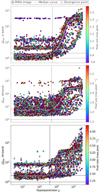 |
Fig. B.1 L-curves of the MiRA images reconstructed using the VLTI/MATISSE 3 Puppis data, and for each spectral band. The median curve resulting from the data binning performed by MYTHRA is shown by the solid black line, and the pink cross indicates the inflection point, corresponding to the optimal hyperparameter value. Each coloured dot represents one of the 3360 reconstructed images generated by the PYRA grid. The colourmap reflects the pixel size value used to reconstruct the circumstellar environment. Top plot : L-band. Centre plot : M-band. Bottom plot : N-band. |
Field of view and angular resolution characteristics probed by VLTI/MATISSE for the observation of 3 Puppis.
Statistic figures obtained with MYTHRA applied on the resulting PYRA grid of 3360 images reconstructed from 3 Puppis data.
Appendix C Comparison between VLTI/MIDI data and VLTI/MATISSE N-band data
Fitted parameters from the chromatic geometric model applied to VLTI/MIDI and VLTI/MATISSE N-band observations of 3 Puppis.
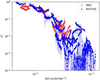 |
Fig. C.1 Comparison in the N-band of the VLTI/MATISSE data (in blue) to the VLTI/MIDI data (in red) of 3 Puppis by plotting their squared visibilities data (V2) in logarithmic scale as a function of spatial frequency. |
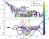 |
Fig. C.2 Comparison in the N-band between the VLTI/MATISSE data of 3 Puppis (in colour gradient from green to yellow), the best-fit MC3D model from Meilland et al. (2010) (in red) composed of a single centred Gaussian component plus an extended background, and the same MC3D model combined with two elliptical Gaussian components (i.e. {MC3D + 2EG} model; in blue) to account for the bright SE asymmetry and the fainter NW model provides a significantly better fit to the MATISSE interferometric observables than the original MC3D model constrained by MIDI data, with a reduced chi-squared of 24 versus 117. Top plot: Squared visibilities (V2) in logarithmic scale as a function of spatial frequency. Bottom plot: Closure phases (CPs) as a function of spatial frequency. |
Appendix D Hydrodynamic framework
Appendix D.1 Approximations adopted
Appendix D.1.1 Mean molecular weight value (μ)
We adopted a mean molecular weight of μ = 2.3, corresponding to the standard value for molecular gas of solar mass composition (i.e. about 70% of hydrogen, 28% of helium, and 2% of heavier elements). This value is widely used in the literature for protoplanetary and circumbinary disc models where the gas is predominantly molecular and weakly ionised (Hayashi 1981; D’Alessio et al. 1998; Draine 2011). The choice of this value was justified by the typical thermochemical conditions in the outer regions of irradiated discs (i.e. temperatures T < 3000 K, densities n > 108 cm−3, and a very low ionisation fraction). Under these conditions, hydrogen is primarily in molecular form (H2), helium remains neutral (He I), and metals are mostly bound in grains or remain singly ionised, yielding a stable effective μ ≃ 2.3. Departures from this value may occur only in highly irradiated, ionised, or dissociative environments.
Appendix D.1.2 Disc locally isothermal
Local isothermality holds when the cooling timescale, tcool, is much shorter than the dynamical (orbital) timescale (i.e. tdyn ≃ Ω−1; with Ω the Keplerian angular frequency). In dusty, irradiated discs such as 3 Pup, the thermal inertia of the gas is low and radiative cooling is efficient due to tight coupling with dust grains. Consequently, temperature fluctuations equilibrate rapidly with the local irradiation field, leading to a vertically isothermal structure at each radius (Ruden & Pollack 1991). Therefore we treated the disc as locally isothermal.
Appendix D.1.3 Geometrically thin disc
The geometrically thin disc approximation holds when the vertical scale height is much smaller than the radial distance, hence an aspect ratio of ε ≪ 1. As shown in Appx. D.2.2, we obtained an aspect ratio of ε ≃ 0.044 at the inner rim (Rrim ~ 3.6 au at 631 pc) and ε ≃ 0.023 at the SE clump position (Rref ~ 10 au at 631 pc). These values are fully consistent with flared, passively irradiated discs in hydrostatic equilibrium and justified the use of the thin disc approximation (Kenyon & Hartmann 1987; Chiang & Goldreich 1997).
Appendix D.1.4 Gaussian vertical density profile (ρ)
We assumed the disc to be locally isothermal and geometrically thin, in line with standard models of circumbinary and proto-planetary discs (Chiang & Goldreich 1997; Dullemond et al. 2001). Under these assumptions, the condition of vertical hydrostatic equilibrium led to a Gaussian vertical distribution of the gas density:

where ρ0 is the midplane density at a given radius (e.g. at the inner rim), z is the vertical coordinate above the midplane, and H is the (pressure) scale height as defined in Eq. D.1.5. This formulation assumed that the temperature is vertically constant and only varies radially (i.e. T = T(R)), consistent with the locally isothermal approximation. This simplification greatly facilitated the thermodynamical and hydrodynamical modelling, and remained valid in the inner ~ 10-20 au of circumbinary discs around evolved B[e] stars, where stellar irradiation dominates over viscous heating.
Appendix D.1.5 Radial thickness (w)
We defined the radial thickness of the SE clump, w, as the local vertical scale height of the disc, under the geometrically thin disc approximation, yielding w ≡ Href. Using the values computed in Appx. D.2.2, we then obtained w - 0.23 au, which defined the natural vertical and radial confinement scale of spiral density waves in hydrostatic equilibrium. This choice avoided overestimating the mass by restricting the integration region to physically meaningful disc layers.
Appendix D.1.6 Angular width (∆φ)
The angular width defines the azimuthal extent of the asymmetric structure identified in the SE quadrant of the disc, referred to as the SE elongated clump (see Sect. 4.1), in the region of Rref. This quantity represents the angular opening of the overdensity along its curved geometry as reconstructed in the MATISSE images (see Fig. 4).
To measure it, we analysed the unconvolved M-band MYTHRA reconstructed image (middle left panel of Fig. 3) by transforming from Cartesian to polar coordinates. In particular, we focused on pixels within the radial interval [Rmin, Rmax] = [13,19] mas, corresponding to the region where the SE elongated clump extends in the M-band image. Then, for each radius, r, within these boundaries, we converted pixel intensities to angular positions, φ, along circles centred on the image centre and with a radius equal to the given r. After collecting all angular pixel values and applying a 3σ threshold to identify robustly clump elements, we finally determined the angular width by subtracting the minimum angular position from the maximum one.
The calculation revealed that the asymmetry spans a well localised arc corresponding to a continuous spiral segment subtending approximately ∆φ ≃ 34° in azimuth. This width was consistent with typical angular spans of spiral arms observed in circumbinary discs with moderate density contrast (e.g. ∆φ ∈ [20, 40]° according to Dong et al. 2015). Therefore, we adopted ∆φ ~ 30° (= π/6 rad) as a representative estimate for the extent of the overdense region.
Appendix D.1.7 Clump area (Aclump)
The total area occupied by the SE clump was computed as a sector of disc annulus at radius Rref, with radial thickness w, and angular width ∆φ, yielding the formulation given in Eq. D.1.9. This definition provided the projected surface area of the clump and allows the estimation of its mass content, Mclump, as a first-order approximation (see Eq. D.1.10).
Appendix D.1.8 Density contrast amplitude (Γ)
The density contrast amplitude is a dimensionless parameter that quantifies the maximum enhancement of the surface density of a spiral arm (e.g. the SE elongated clump) with respect to the local background surface density profile of the disc. Observationally, focusing for instance on the SE elongated clump, the contrast represents the relative intensity of the clump, Iclump, above the intensity level set by the disc background, Ibkd, and can be expressed as Γ = (Iclump - Ibkd)/Ibkd. From our analysis of the M-band MYTHRA image, during the angular width ∆φ measurement, we estimated Γ ~ 20% for the SE clump. In the analytical framework, Γ appears as a model parameter in the spiral density wave equation Σ(R, φ) (see Appx. D.3).
Appendix D.2 Hydrodynamic calculations
Appendix D.2.1 Gravitational instability within the disc
To compute the gravitational stability based on the Toomre theoretical framework (Toomre 1964), whose formula is given in Eq. D.1.4, we first needed to determine the surface density Σrim occupied by the gas at the inner rim, assuming axisymmetric geometry. Using Eq. D.1.1, we obtained a value of Σrim ≃38.2 kg · m−2. We then inferred the angular frequency at the inner rim using Eq. D.1.3, given that the disc material follows Keplerian motion, yielding Ωrim ≃ 9.0 × 10⁻⁸ rad s−1. Finally, the Toomre parameter at the dusty inner rim was Qrim ≃ 2.4 × 10⁴.
Similarly, we wanted to assess the gravitational stability at larger radii, specifically at Rref. In the context of viscously evolving discs, we assumed a power-law surface density profile defined as Σ(R) ∝ R−3/2 (Lynden-Bell & Pringle 1974). Hence, the density at Rref = 10 au (at 631 pc) was inferred as follows:

The corresponding angular frequency gave Ωref ≃ 6.15 × 10⁻⁸ rad · s−1, yielding a Toomre parameter of Qref ≃ 7.5 × 10⁵.
Appendix D.2.2 Verification of the thin disc model for 3 Pup
Under the locally isothermal approximation (see justifications in Appx. D.1) and using the quantities estimated in Appx. D.2.1, we inferred the vertical scale height of the dusty disc at the inner rim through Eq. D.1.5, yielding Hrim ≃ 0.157 au. From Eq. D.1.6, the corresponding aspect ratio at the inner rim was εm ≃ 0.044, which was consistent with values expected for passive irradiated discs in hydrostatic equilibrium, typically ranging between 0.03 and 0.1 (Chiang & Goldreich 1997; Dullemond et al. 2001). This aspect ratio confirmed that the disc geometry supports the thin disc model approximation adopted in deriving the Toomre parameter in Appx. D.2.1. To verify whether this approximation remains valid at larger radii, we extended our analysis to Rref.
Following the same approach, we first computed the angular frequency at Rref using Eq. D.1.3, obtaining Ωref = 6.15 × 10⁻⁸rad · s−1. This yielded a vertical scale height of Href ≃ 0.23 au and an aspect ratio of εref ≃ 0.023. These values demonstrate that while the disc exhibits modest flaring with increasing radius, it remains geometrically thin, from the inner rim out to Rref ~ 10 au, thereby validating our thin disc approximation throughout this region.
Appendix D.2.3 Viscosity evolution and timescale
The disc’s kinematic viscosity was parametrised using the Shakura & Sunyaev (1973) α-prescription as defined in Eq. D.1.7. Adopting a standard viscosity parameter α = 10−2 in the case of moderately turbulent protoplanetary or post-AGB discs (Hartmann 1998; Rafikov 2016), we obtained a viscosity of νrim ≃ 4.98 × 10¹¹ m2 · s−1 at the inner rim, corresponding to a viscous timescale of tvisc,rim ≃ 1.85 × 10⁴ yrs using Eq. D.1.8. Extending this analysis to Rref using the same viscosity law, we found respectively νref ≃ 7.28 × 10¹¹ m2 · s−1 and tvisc,ref -9.75 × 10⁴ yrs. These viscous timescales exceed by more than two orders of magnitude both the orbital period of the central binary (Porb - 137.52 days; see Table 1) and the period inferred for a putative a third body orbiting at Rref (11 yrs; see Sect. 4.4).
Appendix D.2.4 Mass budget of the SE asymmetry
To assess whether the observed SE elongated clump could originate from a bound object, we needed to estimate the total gas mass contained within its area (i.e. in Rref region). We modelled the clump as extending over a sector of angular width ∆φ = 30° and radial thickness w ~ Href (see justifications in Appx. D.1). Using Eq. D.1.9, the defined geometry for the SE clump yielded an area of Aclump ≃ 2.70 × 10²²m2. Combined with the local gas surface density Σref ≃ 8.25 kg · m−2 (see Appx. D.2.1), we obtained a total gas mass enclosed within the clump sector of Mclump ≃ 3.73 × 10⁻² M⊕ ≃ 1.18 × 10⁻⁴ MJup based on Eq. D.1.10 (see justifications in Appx. D.1).
Appendix D.3 Hydrodynamic simulation of a spiral density model
The spiral density wave was defined analytically by a two-dimension model corresponding to the disc’s surface density field Σ(R, φ), in polar coordinates (R, φ), as follows:
![Mathematical equation: \Sigma(R,\phi)&=&\Sigma_0(R) \times \left[\,1+ \Gamma \times \exp \left(-\frac{[\phi-\Phi(R)]^2}{2\, \sigma_\phi^2}\right)\,\right]\\ \mathrm{with} \quad \Phi(R)&=&\phi_0 + \frac{1}{\tan \psi} \times \ln \left(\frac{R}{R_0}\right)\,,](/articles/aa/full_html/2025/12/aa56615-25/aa56615-25-eq32.png)
where ψ is the pitch angle that defines the logarithmic spiral parametrisation, Σ0(R) represents the disc surface density profile (i.e. without the intensity contribution of spiral structure), Γ is the density contrast amplitude of the spiral wave (see definition in Appx. D.1), σφ is the Gaussian azimuthal envelope angular width, R0 is the reference radius, and φ0 is the initial phase of the spiral density wave. The resulting synthetic surface density model with spiral-induced perturbations is shown in Fig. D.1.
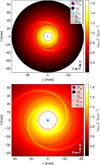 |
Fig. D.1 Synthetic surface density map Σ derived from an analytic spiral density model simulating tidally induced perturbations in the cir-cumbinary disc of 3 Puppis. The model incorporates two trailing spiral arm perturbations caused by the binary companion. The red dashed circle marks the inner dust rim Rrim ≃ 5.7 mas (∼3.6 au at 631 pc), and the black dotted circle indicates the radius of the SE asymmetric structure Rref ≃ 16.71 mas (∼10 au at 631 pc) inferred from the L-band MYTHRA image. Binary star positions are marked with dot symbols (purple for the supergiant star and black for the low-mass companion) scaled to the correct mass ratio and projected separation (stellar radii not to scale). The gas disc extension Dgas ∼ 4.39 mas (∼0.88 au at 631 pc) is displayed as a blue circle to scale. Both panels use logarithmic colour scaling to represent the local gas surface density normalised to 20% contrast. Left plot: Wide FoV (160 mas × 160 mas) in sky-plane Cartesian coordinates (α, δ). Right plot: Same simulation with a FoV matching the VLTI/MATISSE M-band MYTHRA image (87 mas × 87 mas). |
Appendix D.4 Dynamical parameters and physical conditions
Dynamical quantities evaluated at the inner rim (Rrim) and at the distance where the south-eastern asymmetry is (Rref) in 3 Puppis’ disc.
Physical parameters and assumptions adopted for the dynamical analysis of the circumbinary disc around 3 Puppis.
All Tables
List of selected stellar parameters and circumstellar environment properties of the 3 Puppis system from the literature.
Best-fit parameters for the two elliptical Gaussian disc components from the {MC3D + 2EG} model.
VLTI/MATISSE observing log for 3 Puppis performed in low spectral resolution mode (R=30).
Field of view and angular resolution characteristics probed by VLTI/MATISSE for the observation of 3 Puppis.
Statistic figures obtained with MYTHRA applied on the resulting PYRA grid of 3360 images reconstructed from 3 Puppis data.
Fitted parameters from the chromatic geometric model applied to VLTI/MIDI and VLTI/MATISSE N-band observations of 3 Puppis.
Dynamical quantities evaluated at the inner rim (Rrim) and at the distance where the south-eastern asymmetry is (Rref) in 3 Puppis’ disc.
Physical parameters and assumptions adopted for the dynamical analysis of the circumbinary disc around 3 Puppis.
All Figures
|
Fig. 1 Coverage of the (u, v)-plane obtained from the VLTI/MATISSE observations of 3 Puppis. The legend in the lower-right corner indicates the colours corresponding to the four AT configurations used: small (blue), medium (orange), large (green), and extended (red). A schematic map of the VLTI baselines, using the same colour code, is shown in the upper-right corner. East corresponds to increasing x-axis values, and north to increasing y-axis values. |
| In the text | |
|
Fig. 2 VLTI/MATISSE squared visibility data, denoted V2, in logarithmic scale (top plot) and closure phase data, denoted CP, (bottom plot) of 3 Puppis in the L- (blue), M- (green), and N- (red) bands, plotted as a function of spatial frequency B/λ. The vertical dashed lines indicate the approximate positions of the first visibility nulls in the three bands with the same colour code. The horizontal dashed line marks the visibility plateau at long baselines in the L-band, which reflects the relative flux contribution from the unresolved central source. |
| In the text | |
|
Fig. 3 Comparison between the interferometric observables extracted from the MYTHRA averaged images (in blue) and the VLTI/MATISSE data of 3 Puppis (in green), shown respectively in the L-band (first row ), in the M-band ( second row ), and in the N-band ( third row ). Left column : squared visibility amplitudes as a function of spatial frequency in logarithmic scale. Central column : closure phases as a function of spatial frequency, computed using the longest baseline. Right column : final averaged images resulting from MYTHRA, normalised to unity (i.e. the sum over all pixels equals one), with a logarithmic colour scaling, and not convolved with the interferometric beam. The minimum value for each brightness scaling is set to half the standard deviation of the associated image to filter out the artefact produced by the MiRA algorithm. |
| In the text | |
|
Fig. 4 Final image reconstructions of 3 Puppis in the mid-infrared using MiRA, MYTHRA, and SPARCO imaging tools. The FoV for each image is (60 mas × 60 mas) with north up and east left. The dashed blue ellipse indicates the best-fit inner rim of the dusty disc derived from VLTI/AMBER data, while the blue cross marks the SE elongated clump best-fit position, denoted Rref, from MATISSE L-band geometric modelling (at a distance of 16.71 ± 0.03 mas from the image centre). Brightness colour scale is normalised to peak intensity (i.e. maximum pixel value). K-band image : the left-most column shows the images obtained with VLTI/AMBER data by Millour et al. (2011). In the first row the median MiRA image is displayed, and the last two rows present the identical convolved median MiRA image with the λ/2 B max PSF subtraction applied. L-M-N-bands images : the remaining three columns display the images obtained with VLTI/MATISSE. On the first row the resulting MYTHRA averaged image is shown. The second row shows the convolved image of MYTHRA with the λ/2Bmax PSF subtraction applied. The last row gives the resulting SPARCO image, convolved with the interferometric beam. |
| In the text | |
|
Fig. 5 Spectral evolution of the fitted disc parameters from a chromatic two-component geometric model applied to 3 Puppis N-band observations obtained with the VLTI/MIDI (in blue) and VLTI/MATISSE (in orange) instruments. Top plot : the FWHM of the major-axis as a function of wavelength. Bottom plot : elongation (or flattening) ratio as a function of wavelength. |
| In the text | |
|
Fig. 6 Best-fit image at 10 μm using the N-band MATISSE data of 3 Puppis. The fit is performed combining MC3D code with two elliptical Gaussian disc models ({MC3D + 2EG} model) to describe the asymmetries revealed by MYTHRA and SPARCO image reconstructions. The model fitting results in a reduced chi-squared value of 24. East corresponds to increasing x-axis values, and north to increasing y-axis values. |
| In the text | |
|
Fig. 7 Composite image showing the analytic spiral model superimposed on the reconstructed N-band MYTHRA image of 3 Puppis. The logarithmic colour scale represents the observed intensity of the N-band image (normalised to unity and expressed in ADU), while the spiral model is overlaid as a semi-transparent structure representing the local gas surface density normalised to 20% contrast. The red dashed circle marks the inner dust rim (Rrim ≃ 5.7 mas), and the black dotted circle indicates the radius of the SE asymmetric structure (Rref ≃ 16.71 mas) inferred from the L-band MYTHRA image. The curvature and radial extent of the two logarithmic spiral arms closely match the two asymmetries observed in the N-band image, located in the SE and NW regions of the dusty disc. |
| In the text | |
|
Fig. B.1 L-curves of the MiRA images reconstructed using the VLTI/MATISSE 3 Puppis data, and for each spectral band. The median curve resulting from the data binning performed by MYTHRA is shown by the solid black line, and the pink cross indicates the inflection point, corresponding to the optimal hyperparameter value. Each coloured dot represents one of the 3360 reconstructed images generated by the PYRA grid. The colourmap reflects the pixel size value used to reconstruct the circumstellar environment. Top plot : L-band. Centre plot : M-band. Bottom plot : N-band. |
| In the text | |
|
Fig. C.1 Comparison in the N-band of the VLTI/MATISSE data (in blue) to the VLTI/MIDI data (in red) of 3 Puppis by plotting their squared visibilities data (V2) in logarithmic scale as a function of spatial frequency. |
| In the text | |
|
Fig. C.2 Comparison in the N-band between the VLTI/MATISSE data of 3 Puppis (in colour gradient from green to yellow), the best-fit MC3D model from Meilland et al. (2010) (in red) composed of a single centred Gaussian component plus an extended background, and the same MC3D model combined with two elliptical Gaussian components (i.e. {MC3D + 2EG} model; in blue) to account for the bright SE asymmetry and the fainter NW model provides a significantly better fit to the MATISSE interferometric observables than the original MC3D model constrained by MIDI data, with a reduced chi-squared of 24 versus 117. Top plot: Squared visibilities (V2) in logarithmic scale as a function of spatial frequency. Bottom plot: Closure phases (CPs) as a function of spatial frequency. |
| In the text | |
|
Fig. D.1 Synthetic surface density map Σ derived from an analytic spiral density model simulating tidally induced perturbations in the cir-cumbinary disc of 3 Puppis. The model incorporates two trailing spiral arm perturbations caused by the binary companion. The red dashed circle marks the inner dust rim Rrim ≃ 5.7 mas (∼3.6 au at 631 pc), and the black dotted circle indicates the radius of the SE asymmetric structure Rref ≃ 16.71 mas (∼10 au at 631 pc) inferred from the L-band MYTHRA image. Binary star positions are marked with dot symbols (purple for the supergiant star and black for the low-mass companion) scaled to the correct mass ratio and projected separation (stellar radii not to scale). The gas disc extension Dgas ∼ 4.39 mas (∼0.88 au at 631 pc) is displayed as a blue circle to scale. Both panels use logarithmic colour scaling to represent the local gas surface density normalised to 20% contrast. Left plot: Wide FoV (160 mas × 160 mas) in sky-plane Cartesian coordinates (α, δ). Right plot: Same simulation with a FoV matching the VLTI/MATISSE M-band MYTHRA image (87 mas × 87 mas). |
| In the text | |
Current usage metrics show cumulative count of Article Views (full-text article views including HTML views, PDF and ePub downloads, according to the available data) and Abstracts Views on Vision4Press platform.
Data correspond to usage on the plateform after 2015. The current usage metrics is available 48-96 hours after online publication and is updated daily on week days.
Initial download of the metrics may take a while.