© The Authors 2025

1. Introduction

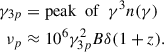
Blazars are a subclass of active galactic nuclei (AGNs) in which a relativistic jet, launched by the central engine, is oriented close to the observer’s line of sight (Blandford & Rees 1978), resulting in highly beamed, rapidly variable, and strongly polarized emission across the entire electromagnetic spectrum (Urry & Padovani 1995). Their spectral energy distributions (SEDs) exhibit two principal components: a low-energy component, with power peaking from the infrared (IR) to the X-ray band, and a high-energy component, which peaks in the γ-rays. In the most widely accepted scenario, the low-energy component is interpreted as synchrotron (S) radiation emitted by ultrarelativistic electrons, while the high-energy bump is attributed either to inverse Compton (IC) emission in purely leptonic models (Blandford & Königl 1979) or to high-energy emission from ultrarelativistic protons in hadronic models (Böttcher et al. 2013). These sources are traditionally classified based on their synchrotron peak frequency (ν_p^S), ranging from low synchrotron-peaked (LSP, ν_p^S < 10¹⁴ Hz) through intermediate synchrotron-peaked (ISP, 10¹⁴ Hz < ν_p^S < 10¹⁵ Hz) to high synchrotron-peaked (HSP, ν_p^S > 10¹⁵ Hz) blazars (Abdo et al. 2010).

The radiation in the S bump is linearly polarized, and the level of the fractional polarization is very low (close to zero) in the low-energy branch, at millimiter frequencies, and reaches a level of tens of percent above the peak of the S bump (Marscher & Jorstad 2022). Moreover, Angelakis et al. (2016), using data from the RoboPol high-cadence polarization-monitoring program (King et al. 2014; Pavlidou et al. 2014), found that for a large sample of γ-ray-loud blazars, the fractional optical polarization depends on ν_p^S showing a limiting envelope, with both the polarization and its dispersion higher in LSP sources than in HSP ones. They also demonstrated that the randomness of the optical electric vector position angle (EVPA) is higher in LSP sources compared to HSP ones.

The synchrotron emission from these sources, extending from radio to X-ray frequencies, provides a unique window into the physical conditions within relativistic jets, including magnetic field structure, particle acceleration mechanisms, and jet dynamics (Marscher 2014). Recent observational advances have dramatically enhanced our ability to probe these phenomena through polarimetric studies spanning from millimeter to X-ray wavelengths. In particular, the launch of the Imaging X-ray Polarimetry Explorer (IXPE) has enabled the first systematic measurements of X-ray polarization in blazars (Weisskopf et al. 2022). IXPE observations of HSP blazars (Liodakis et al. 2022; Di Gesu et al. 2023; Kouch et al. 2024) have revealed X-ray polarization degrees ranging from 10% to 20%, showing a systematic decrease at lower frequencies, with the optical polarization degree systematically larger than the millimiter one. This phenomenology, and the one observed in the RoboPol sample, has been explained by energy stratification of emission regions as electrons lose energy via radiation (Liodakis et al. 2022), providing strong support for shock acceleration models (Kirk et al. 2000) and suggesting a complex multi-zone structure within blazar jets where different energy bands probe distinct physical regions. However, IXPE observations have also revealed EVPA rotations in several blazars (Middei et al. 2023), which present a challenge to simple energy-stratified models that would predict stable, frequency-independent EVPAs if magnetic field configurations remain coherent across emission zones. This discrepancy suggests either that the magnetic field geometry varies significantly between different emission regions or that additional physical processes, such as Faraday rotation or turbulent magnetic field fluctuations, play important roles in determining the observed polarization characteristics.

In this work, we present a comprehensive Monte Carlo framework for modeling multi-zone synchrotron emission in blazar jets, specifically designed to reproduce the energy-dependent polarization characteristics observed from millimeter to X-ray wavelengths. Our approach incorporates spatially resolved emission regions with distinct physical properties, in a purely turbulent framework, that is, we do not assume any correlation between magnetic field and cell size and/or position; we only assume a power-law distribution for the cell size, and we tested different levels of correlation between the size of the cells and cutoff in the electron distribution. This minimal approach aims to provide the most likely statistical characterization of the cell distributions, in terms of size and energy of the electrons, able to reproduce the energy-dependent polarization patterns observed in the millimiter-to-X-ray data for IXPE HPS, and in the optical for the RoboPol dataset. The paper is organized as follows: in Sect. 2.1 we discuss the single-cell S emission, and we provide some useful δ approximations both for the S SED emission and for the fraction polarization. In Sect. 2.2 we investigate analytical trends for the fractional polarization, for the case of a multi-zone scenario, without flux dispersions. In Sect. 2.3, we extend the results of Sect. 2.2 to the case of dispersion of cells flux, and we introduce the concept of flux-weighted effective number of cells contributing to the observed polarization. In Sect. 3.2 we describe the setup for our Monte Carlo (MC) simulation workflow. In Sect. 4 we analyze our MC results for the case of no dispersion on cells’ flux and same cells size (Sect. 4.1), and the case of dispersions on cells’ flux and power-law-distributed cells’ size (Sect. 4.2), presenting the predicted trends for the patterns of the multiwavelength fractional polarization. In Sect. 5 we compare our trends to the multiwavelength trends observed, for a sample of HSP, by IXPE, and to the optical trends observed by RoboPol for a large sample of γ-ray-loud blazars. Finally, in Sect. 6 we discuss our results and present our conclusions.

2. Synchrotron polarization

2.1. Single cell

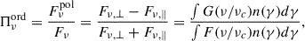
Let us consider a single spherical emitting region, with an ordered magnetic field B, and a population of relativistic electrons, described by energy distribution (EED) n(γ). According to the standard synchrotron (S) theory (Westfold 1959; Rybicki & Lightman 1986), the degree of linear polarization is given by the flux emitted in the directions parallel (F_ν, ∥) and perpendicular (F_ν, ⊥) to the projection of the magnetic field on the plane of the sky,

$$\begin{array}{c}\hfill {\mathrm{\Pi }}_{\nu }^{\mathrm{ord}}=\frac{F_{\nu }^{\mathrm{pol}}}{F_{\nu }}=\frac{F_{\nu ,\perp }-F_{\nu ,\Vert }}{F_{\nu ,\perp }+F_{\nu ,\Vert }}=\frac{\int G(\nu /{\nu }_c)n(\gamma )d\gamma }{\int F(\nu /{\nu }_c)n(\gamma )d\gamma },\end{array}$$(1)

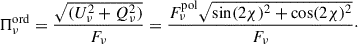
where ν_c is the S critical frequency, and the functions F(x)≡x∫K_5/3(ξ)dξ and G(x)≡xK_2/3(x), are defined in terms of modified Bessel functions of the second kind and fractional order. The S numerical computation, both for the SED and polarization, is performed using the JetSeT¹² code v1.3.1 (Tramacere et al. 2009, 2011; Tramacere 2020). If we assume a reference direction on the sky plane, and χ is the angle between this direction and the projection of the magnetic field on the plane of the sky, then Π_ν^ord can be expressed in terms of Stokes’ parameters:

$$\begin{array}{c}\hfill {\mathrm{\Pi }}_{\nu }^{\mathrm{ord}}=\frac{\sqrt{(U_{\nu }^2+Q_{\nu }^2)}}{F_{\nu }}=\frac{F_{\nu }^{\mathrm{pol}}\sqrt{sin{(2\chi )}^2+cos{(2\chi )}^2}}{F_{\nu }}·\end{array}$$(2)

For a power-law EED, with a spectral index p,

$$\begin{array}{c}\hfill \mathrm{\Pi }(p)=\frac{p+1}{p+7/3}·\end{array}$$(3)

The relation above is valid only for a pure power law, or as long as the S emission is dominated by the power-law branch of the underlying EED. We can obtain a more generic trend, for Eq. (3), by deriving an approximate expression of Π_ν(p) using the standard S theory in δ−function approximation,

$$\begin{array}{c}\hfill \begin{array}{cc}\hfill \nu & \approx {10}^6{\gamma }^{2}B\delta /(1+z)\hfill \\ \hfill F_{\nu }& \approx V\gamma n(\gamma )B{\delta }^3(1+z)/(4\pi d_L{(z)}^2)\hfill \\ \hfill \nu F_{\nu }& \approx V{\gamma }^{3}n(\gamma )B^2{\delta }^4/(4\pi d_L{(z)}^2),\hfill \end{array}\end{array}$$(4)

where z is the cosmological redshift, and δ the beaming factor, V is the volume of the emitting source, and d_L is the luminosity distance. These relations link the flux emitted at a given frequency to the corresponding shape of the electron distribution at γ(ν). The peak frequency of the SED,ν_p, will be at

$$\begin{array}{c}\hfill \begin{array}{cc}\hfill {\gamma }_{3p}& =\mathrm{peak}\mathrm{of}{\gamma }^{3}n(\gamma )\hfill \\ \hfill {\nu }_p& \approx {10}^6{\gamma }_{3p}^{2}B\delta (1+z).\hfill \end{array}\end{array}$$(5)

Assuming that EED is a power-law with an exponential cutoff,

$$\begin{array}{c}\hfill \begin{array}{cc}\hfill n(\gamma )& =K{\gamma }^{-p}exp(-\gamma /{\gamma }_{\mathrm{cut}})\hfill \\ \hfill {\gamma }_{3p}& ={\gamma }_{\mathrm{cut}}(3-p),\mathrm{for}p<3\hfill \\ \hfill {\nu }_p& \approx {10}^6{{\gamma }_{\mathrm{cut}}(3-p)}^{2}B\delta (1+z).\hfill \end{array}\end{array}$$(6)

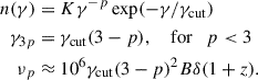
By using the δ−function approximation, the energy-dependent slope, $p_{\nu }^{(\delta )}$, can be evaluated as the log-derivative of n(γ) at γ(ν),

$$\begin{array}{c}\hfill p_{\nu }^{(\delta )}=\frac{dlogn(\gamma )}{dlog\gamma }{|}_{\gamma (\nu )}\end{array}$$(7)

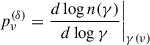
or, conversely, $p_{\nu }^{(\delta )}$ can be estimated from F_ν as

$$\begin{array}{c}\hfill p_{\nu }^{(\delta )}=2\frac{dlogF(\nu )}{dlog\nu }+1.\end{array}$$(8)

Finally, the δ−function approximation for the fractional polarization can be obtained from Eq. (3):

$$\begin{array}{c}\hfill {\mathrm{\Pi }}_{\nu }^{\delta }=\mathrm{\Pi }(p_{\nu }^{(\delta )}).\end{array}$$(9)

In Figure 1, we show a comparison for Π_ν^ord using the different methods described above. The row-a panel shows the S SED, and the row-b panel the corresponding fractional polarization as a function of the frequency, for a power-law cutoff EED, for γ_cut = 5 × 10⁴, γ_min = 2, and p = [1.5, 2.0, 2.5]. We notice that the exact calculation of Π_ν^ord, evaluated using Eq. (1), and marked by solid lines, is well approximated by the δ−approximation from Eq. (9), both using $p_{\nu }^{\delta }$ from Eq. (7) (solid circles), and using $p_{\nu }^{\delta }$ from Eq. (8) (crosses). The fractional deviation of the two δ-approximation methods, reported in the c-row panel of Figure 1, reaches a maximum value of a few percents, with the method using $p_{\nu }^{\delta }$ from Eq. (8) providing a better performance compared to $p_{\nu }^{\delta }$ from Eq. (7). We also notice the asymptotic behavior of Π_ν^ord: below ν_pΠ_ν^ord asymptotically approaches the value dictated by Eq. (3) (horizontal dashed lines), whilst, above ν_p it deviates significantly from the Eq. (3), asymptotically approaching the maximal polarization limit of 1.0, for ν/ν_p > > 1. More in detail, if we define the polarization slope, a, as the log-derivative:

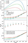Fig. 1. Left panels: The S SED (row a), and the corresponding fractional polarization (row b) as a function of the frequency, for a power-law cutoff EED, γcut = 5 × 104, and p = [1.5, 2.0, 2.5]. The solid lines in the row b panel mark the Πνord evaluated using Eq. (1), the circles mark the δ approximation from Eq. (9) using $p_{\nu }^{(\delta )}$ from Eq. (7), and the crosses using $p_{\nu }^{(\delta )}$ from Eq. (8). The dashed lines mark the asymptotic power-law trend from Eq. (3). The relative error for the δ-approximation methods, w.r.t. the exact method (row c). In the row d panel, we report the best-fit of Πνord by means of a broken power-law function.

$$\begin{array}{c}\hfill a=\frac{dlog{\mathrm{\Pi }}_{\nu }^{\mathrm{ord}}(\nu )}{dlog\nu }\end{array}$$(10)

and we fit Π_ν^ord by means of a broken power-law, we notice that Π_ν^ord, below ν_p, asymptotically approaches a value of a_l ≈ 0, above ν_p reaches a value of a_h ≈ [0.02, 0.03]. The maximum value of a is limited by the log-ratio of the maximum excursion of polarization (typically [0.75 − 1]) to the maximum SED excursion in frequency above ν_p (typically a few decades, depending on the EED).

2.2. Synchrotron polarization: case of N cells with no dispersion on flux

Now, let’s consider a system of N_c cells, with N_ν ≤ N_c indicating the number of cells emitting at the frequency ν. In each cell, the magnetic field is ordered, but the single-cell position angle, χ_i^r, is randomly oriented, and F_ν, i is the single-cell flux. We assume that the pitch angle (the angle between an electron’s velocity vector and the direction of the magnetic field), in each cell, it can be either fixed or distributed uniformly, without any loss of generality, since in the former case the term in sin(α) can be factored out in Eq. 1, and in the latter, the average of a uniform distribution of α, does not change the results compared to the fixed angle case. For the specific case of almost identical cells, that is, $F_{\nu ,i}\approx {\overline{F}}_{\nu }$, and $F_{\nu ,i}^{\mathrm{pol}}\approx {\overline{F}}_{\nu }^{\mathrm{pol}}$, the average degree of the linear S polarization (⟨Π_ν⟩), at a given frequency, can be evaluated as in Marscher & Jorstad (2022):

$$\begin{array}{cc}\hfill ⟨{\mathrm{\Pi }}_{\nu }⟩& ={\mathrm{\Pi }}_{\nu }^{\mathrm{ord}}{\overline{F}}_{\nu }\langle \frac{\sqrt{{(\sum _i^{N_{\nu }}sin(2{\chi }_i^r))}^2+{({\displaystyle \sum _i^{N_{\nu }}}cos(2{\chi }_i^r))}^2}}{{\displaystyle {\sum }_i^{N_{\nu }}}{\overline{F}}_{\nu }}\rangle \hfill \\ \hfill & \approx \frac{{\mathrm{\Pi }}_{\nu }^{\mathrm{ord}}}{\sqrt{N_{\nu }}}.\hfill \end{array}$$(11)

We can also define a polarization factor, as in Marscher & Jorstad (2022):

$$\begin{array}{c}\hfill {\kappa }_{\nu }=\sqrt{f_{\mathrm{ord}}^2+\frac{{(1-f_{\mathrm{ord}})}^2}{N_{\nu }}}\end{array}$$(12)

where f_ord is the fraction of coherent magnetic field in the system, which reduces to ${\kappa }_{\nu }=\frac{1}{\sqrt{N_{\nu }}}$, for f_ord = 0. In the following, we investigate the case of f_ord = 0, hence, all the results presented in the following can be easily rescaled to the case of 0 < f_ord ≤ 1.

2.3. Synchrotron polarization: Case of N cells with dispersion on flux

In a more general and realistic scenario, the flux of each cell, F_ν, i, depends on the physical properties of each cell, that is, $F_{\nu ,i}\ne {\overline{F}}_{\nu }$, preventing the F_ν term from being factored out in Eq. 11 :

$$\begin{array}{c}\hfill {\mathrm{\Pi }}_{\nu }=\frac{\sqrt{{({\displaystyle \sum _i^{N_{\nu }}}{F}^{{}_{\nu ,i}}{\mathrm{\Pi }}_{\nu ,i}sin2{\chi }_i)}^2+{({\displaystyle \sum _i^{N_{\nu }}}{F}_{\nu ,i}{\mathrm{\Pi }}_{\nu ,i}cos2{\chi }_i)}^2}}{{\displaystyle {\sum }_i^{N_{\nu }}}{F}_{\nu ,i}}·\end{array}$$(13)

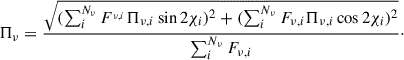
This implies that the effective number of emitting cells at a given frequency will depend on the statistical distribution of the physical parameters of the cells in the system. From a statistical standpoint, the effective number of emitting cells can be interpreted as the effective sample size (ESS) in a sample with weights (w_i), using the approach of Shook-Sa & Hudgens (2022):

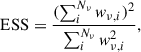$$\begin{array}{c}\hfill \mathrm{ESS}=\frac{{({\displaystyle {\sum }_i^{N_{\nu }}}{w}_{\nu ,i})}^2}{{\displaystyle {\sum }_i^{N_{\nu }}}{w}_{\nu ,i}^2},\end{array}$$(14)

where the cell weights, for Eq. (13), are defined as:

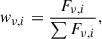$$\begin{array}{c}\hfill w_{\nu ,i}=\frac{F_{\nu ,i}}{{\displaystyle \sum F_{\nu ,i}}},\end{array}$$(15)

hence, the effective number of cells contributing to a given frequency, $N_{\nu }^{\mathrm{eff}}$, will read:

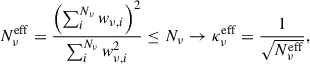$$\begin{array}{c}\hfill N_{\nu }^{\mathrm{eff}}=\frac{{\left({\displaystyle {\sum }_i^{N_{\nu }}}{w}_{\nu ,i}\right)}^2}{{\displaystyle {\sum }_i^{N_{\nu }}}{w}_{\nu ,i}^2}\le N_{\nu }\to {\kappa }_{\nu }^{\mathrm{eff}}=\frac{1}{\sqrt{N_{\nu }^{\mathrm{eff}}}},\end{array}$$(16)

and the average frequency-dependent fraction polarization will read:

$$\begin{array}{c}\hfill ⟨{\mathrm{\Pi }}_{\nu }⟩\approx \frac{⟨{\mathrm{\Pi }}_{\nu }^{\mathrm{ord}}⟩}{\sqrt{N_{\nu }^{\mathrm{eff}}}}={\kappa }_{\nu }^{\mathrm{eff}}⟨{\mathrm{\Pi }}_{\nu }^{\mathrm{ord}}⟩.\end{array}$$(17)

We stress that our definition of $N_{\nu }^{\mathrm{eff}}$ provides a more robust estimate of the flux-weighted cell contribution to the total fractional polarization compared to that presented in Peirson & Romani (2019), being the latter defined as the number of zones contributing half of the integrated flux.

The relevant result here is that the observed fractional polarization, in general, will not depend on N_ν, but on $N_{\nu }^{\mathrm{eff}}$. As a consequence, the estimate of N_ν (or N_c), from (Π_ν^ord/⟨Π_ν⟩)² will lead to an underestimation of the actual number of cells in the system.

3. Simulation setup and workflow

3.1. MC simulations setup

In a turbulent medium, even though we might have similar cell sizes, the EED, the beaming factor, and other parameters can change. We need to accurately compute the S emission and polarization for each cell and generate the individual cell properties via a Monte Carlo approach. We assume that our system has a spherical geometry, with a characteristic radius, R_S, and that the single-cell radius, R_c, is distributed as a power-law, with index q, via the scaling factor r, according to:

$$\begin{array}{c}\hfill \begin{array}{cc}\hfill r& \sim r^q,q\le 0,0<r_{\min }<r<r_{\max }\le 1\hfill \\ \hfill f_{R_c}& =r^q{R}_S\hfill \end{array}\end{array}$$(18)

we set R_S = 10¹⁶ cm. The cell values of the magnetic field intensity, B_c, and of the beaming factor, δ_c, are distributed as a flat PDF or have a fixed value:

$$\begin{array}{c}\hfill \begin{array}{cc}\hfill f_{{\delta }_c}& =\mathcal{U}[{\delta }_{\min },{\delta }_{\max }],\mathrm{or}{f}_{{\delta }_c}={\delta }_0\hfill \\ \hfill f_{B_c}& =\mathcal{U}[B_{\min },B_{\max }],\mathrm{or}{f}_{B_c}=B_0.\hfill \end{array}\end{array}$$(19)

The position angle of the magnetic field, in a single cell, χ_c^r, is randomly oriented: f_χc^r = 𝒰[0, 2π].

The EED is assumed to be a power-law with an exponential cutoff:

$$\begin{array}{c}\hfill n(\gamma )=K{\gamma }^{-p}exp(-\gamma /{\gamma }_{\mathrm{cut}}),\end{array}$$(20)

the cell values of the index EED index, p_c, are distributed as a uniform distribution, or have a fixed value:

$$\begin{array}{c}\hfill f_{p_c}=\mathcal{U}[p_0,p_0+\mathrm{\Delta }p],\mathrm{or}{f}_{p_c}=p_0.\end{array}$$(21)

We investigated four different scenarios for the PDF of γ_cut, f_γcut: a scenario with a fixed value of γ_cut:

$$\begin{array}{c}\hfill {\delta }_f:f_{{\gamma }_{\mathrm{cut}}}={\gamma }_{\mathrm{cut}}^{\mathrm{ref}}\end{array}$$(22)

and a scenario with dispersion on γ_cut. For the latter scenario, two distributions have no correlation between cell size and γ_cut:

$$\begin{array}{c}\hfill \begin{array}{cc}\hfill \mathit{uniform}:f_{{\gamma }_{\mathrm{cut}}}& =\mathcal{U}[{\gamma }_{\mathrm{cut}}^{\mathrm{LB}},{\gamma }_{\mathrm{cut}}^{\mathrm{ref}}]\hfill \\ \hfill log-uniform:f_{{\gamma }_{\mathrm{cut}}}& =\mathcal{U}[log({\gamma }_{\mathrm{cut}}^{\mathrm{LB}}),log({\gamma }_{\mathrm{cut}}^{\mathrm{ref}})]\hfill \\ \hfill & =\frac{1}{{\gamma }_{\mathrm{cut}}log({\gamma }_{\mathrm{cut}}^{\mathrm{ref}}/{\gamma }_{\mathrm{cut}}^{\mathrm{LB}})}\propto {\gamma }_{\mathrm{cut}}^{-1}\hfill \end{array}\end{array}$$(23)

and the third one establishes a linear relationship between R_c and γ_cut, setting ${\gamma }_{\mathrm{cut}}^{\min .\mathrm{ratio}}=r_{\min }$ and ${\gamma }_{\mathrm{cut}}^{\mathrm{ref}}=r_{\max }$, and applying the transformation ${\gamma }_{\mathrm{cut}}\propto {\gamma }_{\mathrm{cut}}^{\mathrm{ref}}r$, leading to:

$$\begin{array}{c}\hfill \mathit{linear}:f_{{\gamma }_{\mathrm{cut}}}\propto \frac{{\gamma }_{\mathrm{cut}}^q}{{({\gamma }_{\mathrm{cut}}^{\mathrm{ref}})}^{q+1}}.\end{array}$$(24)

The dispersion on γ_cut is controlled by the value of the lower bound defined as ${\gamma }_{\mathrm{cut}}^{\mathrm{LB}}$, as $max(100,{\gamma }_{\mathrm{cut}}^{\mathrm{ref}}{\gamma }_{\mathrm{cut}}^{\min .\mathrm{ratio}})$, implying that lower values of ${\gamma }_{\mathrm{cut}}^{\min .\mathrm{ratio}}$ lead to a larger dispersion. The linear distribution is motivated by results from magnetic reconnection Particle-in-Cell (PIC) simulations (Li et al. 2023; Sironi et al. 2016), finding the EED high-energy cutoff scaling linearly with the plasmoids’ width. We notice that for q < 0 both the log-uniform and linear cases result in f_γcut being a decreasing function of γ_cut, with the relevant difference that the linear case introduces a positive correlation between the cell size and the value of f_γcut.

3.2. MC simulations workflow

For each combination of the input parameters described in Sect. 3.1, we first perform a calibration stage, that is, we calibrate N_c and ${\gamma }_{\mathrm{cut}}^{\mathrm{ref}}$, to obtain a trial-averaged optical polarization fraction, ⟨Π_ν^opt⟩, within [0.4 − 0.5]%, and a trial-averaged value of ν_p^S within=[0.8 − 1.2]×10¹⁷ Hz. As a reference value for the optical frequency, we use the value of 5 × 10¹⁴ Hz. Details of the calibration stage are reported in Sect. A. At the end of the calibration stage, the calibrated values of N_c and ${\gamma }_{\mathrm{cut}}^{\mathrm{calib}}$ are used for the full MC simulations as follows:

• we define six bins for ν_p^S, evenly spaced in the logarithm, over the range [${\nu }_{p,\min }^S={10}^{12}$, ${\nu }_{p,\max }^S={10}^{18}$] Hz. Each value of ν_p, i^S is mapped to a corresponding bin for the EED cutoff energy of ${\gamma }_{\mathrm{cut},i}^{\mathrm{ref}}$, by scaling the calibrated value of ${\gamma }_{\mathrm{cut}}^{\mathrm{calib}}$ according to the third of Eq. (6).

• For each bin of γ_cut, i we run 1000 trials using always the same value of N_c, and drawing ${\gamma }_{\mathrm{cut}}^{\mathrm{ref}}$ from $\mathcal{U}[{\gamma }_{\mathrm{cut},i}^{\mathrm{ref}},{\gamma }_{\mathrm{cut},\mathrm{i}+1}^{\mathrm{ref}}]$.

• For each run, we verify that the sample variance converges according to Stein’s two-stage scheme (Stein 1945) as implemented in Wübbeler et al. (2010). In detail, we have verified, for each run, that the interval, [⟨Π_ν⟩(1 − ε_MC),⟨Π_ν⟩(1 + ε_MC)], for ε_MC ≤ 0.15, provides confidence interval for the true value of Π_ν, at a confidence level of 0.95, up to ν ≤ 1000 × ν_p.

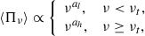
At the end of the MC, we have 1000 realizations for each of the six ν_p^S bins, where the only changed parameter per bin is ${\gamma }_{\mathrm{cut}}^{\mathrm{ref}}$, that is, each trial and each bin of ν_p^S, has the same value of N_c and the same PDFs f_Rc, f_δc, f_Bc, and f_χ^r. The trials are eventually binned according to the $⟨{\nu }_p^S⟩$ value in the ν_p, i^S bins, and the relevant statistics of the parameters are extracted.

4. Simulation trends

In this section, we provide a statistical description of the ⟨Π_ν⟩ trends, for two different scenarios: the case of cells with the equal size (Sect. 4.1) and the case of power-law-distributed cell sizes (Sect. 4.2). We aim to do the following:

• verify the ⟨Π_ν⟩ trend provide by Eq. (17) and in particular the connection between the polarization factor κ_ν^eff and $N_{\nu }^{\mathrm{eff}}$.

• characterize the ⟨Π_ν⟩ trends as a function of ν/ν_p.

• identify how the different PDFs for f_Rc, f_δc, f_Bc, and f_γcut impact the trends.

4.1. Case of equal-size cells

We start by investigating the case of equal-size (ES) cells with three different configurations, whose parameters are summarized in Table 1. In Figure 2 we show the impact, on the frequency-dependent polarization pattern ⟨Π_ν⟩, of different levels of randomization, from configuration ES1 to ES3. The left column panels refer to the case of identical cells, i.e., the configuration ES1 of Table 1. The middle column panels refer to the configuration ES2, i.e. same as ES1 but using for f_γcut the log-uniform PDF and, finally, the right column panels refer to the ES3 case, with the same configuration as for the ES2 case, but adding a uniform PDF, for p, f_p ∼ 𝒰[1.8, 2.8]. For all the cases, we use ${\gamma }_{\mathrm{cut}}^{\min .\mathrm{ratio}}=0.1$.

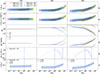Fig. 2. Different colors identifying the corresponding νp bins, which are the same for all the panels. Top panels: Left column: case of identical cells (configuration ES1 in Table 1). Middle column: case of configuration ES2 in Table 1, i.e. using fγcut = log-uniform. Right column: panel, case of configuration ES3, same as ES2 but adding a flat PDF, for p : fp ∼ 𝒰[1.8, 2.8]. All the trends are reported versus ν/νp. Solid lines mark the MC 0.5 quantiles and shaded areas mark the 1-σ quantiles dispersion, for the MC trials. Row a: the trend of the ratio of ⟨Πν⟩. Row b: same as for Row 1, but for trials-averaged trends for ⟨Πν⟩/⟨Πνord⟩. Row c: trials-averaged trends for Nν (dashed lines) and $N_{\nu }^{\mathrm{eff}}$ (solid lines). Row d: trials-averaged trends for κν (dashed line) and κνeff (solid lines). Row e: SEDs for the νp bin = [1016 − 1017] Hz, the dashed vertical line shows the ν/νp value, above which not all the cells contribute to the SED flux. The dot-dashed vertical lines mark ν = νpmin, where νpmin is the SED peak value for the lowest flux cell.

The trends for the ratio of ⟨Π_ν⟩ and ⟨Π_ν⟩/⟨Π_ν^ord⟩ are shown in the panels of row a and b, respectively, where the shaded area represents the 1-σ quantiles dispersion for the MC trials, and the solid line represents the median value. The different colors identify the corresponding ν^p bins, and are the same for all the panels. The c-row panels show the trends for the trials-averaged value of $N_{\nu }^{\mathrm{eff}}$, and the d-row panels the trials-averaged trends for the polarization factor κ_ν (dashed line) and κ_ν^eff (solid lines). The SEDs for the case ν_p bin = [10¹⁶ − 10¹⁷] Hz are represented in the e-row panels, where the shaded area encompasses the entire MC range. The dot-dashed vertical lines mark the SED peak value for the lowest flux cell,ν = ν_p^min, and the dashed vertical lines the ν/ν_p value above which not all the cells contribute to the SED flux. It is clear that for the case of identical cells (ES1), N_ν and $N_{\nu }^{\mathrm{eff}}$ coincide, and this translates to κ_ν = κ_ν^eff. In contrast, by adding a randomization on γ_cut (middle column,ES2), we start to introduce a modulation on $N_{\nu }^{\mathrm{eff}}$, with $N_{\nu }^{\mathrm{eff}}<N_{\nu }$ for ν ≥ ν_p^min, leading to a difference between the polarization factor, with κ_ν^eff > κ_ν, for ν ≥ ν_p^min. This modulation is not only related to the fact that above a given γ_cut only a few cells are contributing, as demonstrated by the dashed lines trends related to κ_ν, but mostly to the impact of the different cell flux contribution, which is shown by the κ_ν^eff trend. This modulation introduces a turnover in $N_{\nu }^{\mathrm{eff}}$ and consequently in κ_ν^eff and ⟨Π_ν⟩, located around ν ≳ ν_p^min. The turnover still persists when we introduce a randomization on p (left column, ES3). We model the ⟨Π_ν⟩ trend by means of a broken power-law function:

$$\begin{array}{c}\hfill ⟨{\mathrm{\Pi }}_{\nu }⟩\propto \{\begin{array}{cc}{\nu }^{a_l},\hfill & \nu <{\nu }_t,\hfill \\ {\nu }^{a_h},\hfill & \nu \ge {\nu }_t,\hfill \end{array}\end{array}$$(25)

with a_l and a_h, indicating the low and high-energy indices, respectively, and ν_t the turnover frequency, capturing the ν_p^min position. In the following, we analyze the trends of a_l and a_h, focusing on the ν_p bin = [10¹⁶ − 10¹⁷] Hz (rows e and f of Figure 2), and we find:

• For the ES1 configuration, since $N_{\nu }^{\mathrm{eff}}\approx N_{\nu }\approx N_c$, the value of the two power-law indices, a_l ≈ 0 and a_h ≈ 0.03 reflect the single-cell polarization trend, as reported in the bottom panel of Figure 1, i.e. asymptotically equal to the value from Equation (3), for ν < ν_p^min (γ < γ_3p) and mildly increasing for ν > ν_p^min (γ > γ_3p).

• For the ES2 configuration, the trend below ν_p^min is the same as for ES1, since there is no modulation on $N_{\nu }^{\mathrm{eff}}$ below ν_p, on the contrary, above ν_p^min the modulation on $N_{\nu }^{\mathrm{eff}},$ introduced by the dispersion on γ_cut, leads to a significant hardening of a_h ≈ 0.15. We notice that such a large value of a_h is incompatible with the low value obtained for the single-cell configuration (a_h ≲ 0.03), which hints that a significant dispersion is required in γ_cut (and consequently on γ_3p and ν_p), to reproduce it.

• For the ES3 configuration, the trends above ν_p^min are similar to the case of ES2, with a_h ≈ 0.17, on the contrary, below ν_p^min, the dispersion on p introduces a low-energy slope a_l ≈ 0.05, which is significantly larger than the value of a_l ≈ 0.01 observed for the case of no dispersion on p (ES1 and ES2). The value of the slope a_l relates to the dispersion of p, and will be investigated in more detail in the next subsection.

In conclusion, the results of the ES scenario indicate that the slope of the high-frequency polarization is mainly influenced by the modulation of $N_{\nu }^{\mathrm{eff}}$ above ν_p^min, driven by the dispersion in γ_cut. On the other hand, the low-frequency slope a_l is significantly affected by the dispersion on p. This behavior highlights the interplay between the EED parameters and the resulting polarization patterns, emphasizing the importance of accurately modeling the underlying physical properties of the emitting cells to interpret observational data effectively.

4.2. Case of power-law-distributed cell sizes

In this section, we extend the parameter space investigated in the previous section by considering the case of cells distributed according to a power law, testing different f_γcut distributions and different levels of dispersion on f_pc. In total, the power-law (PL) scenario counts 780 different configurations, obtained by combining the different PDF configurations listed in Table 2. Our goal is to investigate the impact of f_Rc, f_γcut, and f_pc on the values of a_l and a_h. We fit the 0.5 quantiles of the ⟨Π_ν⟩ obtained for each run using Eq. (25) and leaving all the parameters free. In Figure 3, we show the resulting trends of a_l (left panels) and a_h (right panels), as functions of Δ_p (top panels), r_min (middle panels), and ${\gamma }_{\mathrm{cut}}^{\min .\mathrm{ratio}}$ (bottom panels). Our findings on the values of a_h and a_l are summarized as follows:

• a_l: Consistent with the ES configuration, we find that the average value of a_l increases with the dispersion in p, and is largely independent of r_min and ${\gamma }_{\mathrm{cut}}^{\min .\mathrm{ratio}}$. However, for the case of log-uniformf_γcut, a_l decreases as ${\gamma }_{\mathrm{cut}}^{\min .\mathrm{ratio}}$ increases. This is expected since $f_{{\gamma }_{\mathrm{cut}}}\propto {\gamma }_{\mathrm{cut}}^{-1}$ and the cell size is uncorrelated with γ_cut; thus, lower values of ${\gamma }_{\mathrm{cut}}^{\min .\mathrm{ratio}}$ lead to a larger dispersion in cell flux weights at low frequencies, increasing $N_{\nu }^{\mathrm{eff}}$, with a consequent hardening of the slope of the polarization factor below ν_p. In contrast, for the linear case, the positive correlation between r and γ_cut compensates for the decreasing probability of cells with large γ_cut with the larger size of the same cells, mitigating the flux weight dispersion at low frequencies, and making the a_l slope of the polarization factor insensitive to ${\gamma }_{\mathrm{cut}}^{\min .\mathrm{ratio}}$.

• a_h: The high-energy slope of the polarization factor, unlike a_l, is independent of Δ_p, and generally also of r_min, since these parameters do not affect the modulation of $N_{\nu }^{\mathrm{eff}}$ above the turnover frequency. Also ${\gamma }_{\mathrm{cut}}^{\min .\mathrm{ratio}}$ does not impact the trends, since its impact on ν_p^min is captured by the ν_t free parameter.

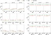Fig. 3. Summary of the polarization slope trends for the PL-distributed parameter space reported in Table 2. Each subpanel refers to the three different values of q = [0, −1.0, −1.5], as reported in the subpanel title. Top panels: Low-energy (al, left panels) and high-energy (ah, right panels) polarization slopes as a function of the dispersion in the electron energy distribution index, Δp. Middle panels: al and ah as a function of the minimum cell size ratio, rmin. Bottom panels: al and ah as a function of the minimum cutoff ratio, ${\gamma }_{\mathrm{cut}}^{\min .\mathrm{ratio}}$. Different colors correspond to the different fγcut PDF reported in the top legend.

Finally, in the left panel of B.1 we show the trend of the effective flux-averaged, $N_{\nu }^{\mathrm{eff}}$, at the reference frequencies used for the millimiter (2 × 10¹¹ Hz), optical (5 × 10¹⁴ Hz), and X-ray (1 × 10¹⁸ Hz) frequencies, and in the top panel of Figure B.2, we show how the number of N_c exceeds, at least by a factor of 10, the value of $N_{\nu }^{\mathrm{eff}}$. The upper value of $N_c/N_{\nu }^{\mathrm{eff}}$ reaches up to a few thousand, for the X-ray frequency, and decrease to a few hundred for the optical frequency, and up to a few tens for millimiter frequency. The effect is larger for steeper values of q.

In summary, the low-frequency polarization slope a_l is most sensitive to the dispersion in p, while the high-frequency slope a_h is mainly set by the decrease in the effective number of emitting cells above the SED peak, driven by the dispersion ob γ_cut, and is less sensitive to the parameters related to the low-energy branch of the EED.

5. Comparison with observed data

In this section, we compare the results of our simulations for the case of PL-distributed cell size, discussed in the previous section, with the observed data. We test the following features, observed in the phenomenology:

• The Π_ν trend observed by IXPE for HPS objects, resulting in the X-ray polarization degrees on the order of 10–20%, with a systematic decrease at lower frequencies, with the optical polarization degree systematically larger than the millimiter one. This trend is shown in the right panel of Figure 4. The sample refers to the millimiter-to-X-ray Π_ν trends (dashed lines) for Mrk 421, Mrk 501, PKS2155-304, 1ES0229+200, and 1ES1959+650, collected from recent IXPE multiwavelength campaigns (Liodakis et al. 2022; Di Gesu et al. 2023; Kouch et al. 2024; Middei et al. 2023). The solid blue line represents a broken-power-law fit to the data, returning a millimiter-to-optical polarization index of a_mm − o ≈ 0.1, and an optical-to-X-ray index of a_o − X ≈ 0.17.

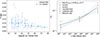
  Fig. 4. Left panel: The limiting envelope, found by RoboPol (Angelakis et al. 2016), for a large sample of γ-ray-loud blazars between νpS and both the average fractional optical polarization and its dispersion. Right panel: The Πν trend observed in by IXPE for the HPS Mrk 501, Mrk 421, PKS2155-304, 1ES0229+200, and 1ES1959+650 collected from recent IXPE multiwavelength campaigns (Liodakis et al. 2022; Di Gesu et al. 2023; Kouch et al. 2024; Middei et al. 2023).

• The limiting envelope, found by RoboPol (Angelakis et al. 2016) for a large sample of γ-ray-loud blazars, between ν_p^S and both the average fractional optical polarization and its dispersion (left panel of 4), and between ν_p^S and the EVPA.

5.1. IXPE HPS ⟨Π_ν⟩ trends

To compare the HSP Π_ν trends observed by IXPE with our simulations, we perform the same analysis as in Sect. 4.2, but we select only the MC runs for 10 × 15 Hz ≤ ν_p^S ≤ 10 × 18 Hz, and in place of estimating a_l and a_h using the best-fit values returned by Eq. (25) with all the parameters free, we compute directly the indices a_{millimiter − o} and a_o − X using the reference values for the millimiter, optical, and X-ray frequencies, of 2 × 10¹¹ Hz, 5 × 10¹⁴ Hz, and 1 × 10¹⁸ Hz, respectively.

The shaded areas in Figure 5, represent the ±20% boundary for the observed values of a_mm − o and of a_o − X, and the solid lines represent the results of our MC simulations, with the error bar indicating the 2-σ confidence quantiles.

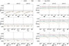Fig. 5. Summary of polarization slope trends for the PL-distributed parameter space reported in Table 2, for the HSP objects, selecting MC runs with (10 × 15 Hz ≤ νpS ≤ 10 × 18 Hz). Top panels: Low-energy (amm − o, left panels) and high-energy (ao − X, right panels) polarization slopes as a function of the dispersion in the electron energy distribution index, Δp. Middle panels: al and ah as a function of the minimum cell size ratio, rmin. Bottom panels: al and ah as a function of the minimum cutoff ratio, ${\gamma }_{\mathrm{cut}}^{\min .\mathrm{ratio}}$. Different colors and line styles correspond to the various PDFs parameter configurations as indicated in the legend and in the titles of the panels.

Although the a_mm − o index samples ⟨Π_ν⟩ below the optical frequency, which is typically below the peak frequency of the HSP objects, the pattern is similar to the one obtained for a_l, since the modulation in $N_{\nu }^{\mathrm{eff}}$ does not change below ν_p^S. Consistent with a_l, we find that the most relevant parameters for the a_mm − o index are the dispersion on p, which is positively correlated with a_mm − o, and the value of ${\gamma }_{\mathrm{cut}}^{\min .\mathrm{ratio}}$, which has a negative correlation, for f_γcut = log-uniform. In general, the observed data favor a dispersion Δ_p ⪆ 1, and values of ${\gamma }_{\mathrm{cut}}^{\min .\mathrm{ratio}}⪅0.1$ for the case of f_γcut = log-uniform. We also notice that the log-uniform distribution provides the best match with the data.

The a_o − X index shows a different trend compared to a_h, for r_min ≈ 1, for the case of linearf_γcut, and for values of ${\gamma }_{\mathrm{cut}}^{\min .\mathrm{ratio}}⪆.1$, for all the f_γcut distributions. The different behavior between a_h and a_o − X comes from the fact that a_h depends on the modulation of $N_{\nu }^{\mathrm{eff}}$ above ν_p^min. For the a_l case, the modulation on ν_p^min, driven by the dispersion on γ_cut, is captured by the ν_t free parameter. In contrast, in the case of a_o − X, the value of ν_t is fixed to the value of 5 × 10¹⁴ Hz. As a consequence, the modulation on ν_p^min, driven by ${\gamma }_{\mathrm{cut}}^{\min .\mathrm{ratio}}$, places the optical frequency below the actual value of ν_t, leading to a softening of a_o − X, compared to a_h. This effect increases for lower values of ${\gamma }_{\mathrm{cut}}^{\min .\mathrm{ratio}}$. This results in a significant tension with the data for r_min ≈ 1, for the case of linearf_γcut, and for values of ${\gamma }_{\mathrm{cut}}^{\min .\mathrm{ratio}}\approx 1$, for all the f_γcut distributions, improving the constraining power of a_o − X.

5.2. RoboPol limiting envelope

To test whether the samples generated in our MC are statistically compatible with the RoboPol observed trend, we use a two-dimensional two-sample Kolmogorov–Smirnov (KS) test, where the two independent variables are ν_p^S and Π_opt (evaluated at 5 × 10¹⁴ Hz). The KS test is performed using the public code NDTEST³, and crosschecked against the public code 2DKS⁴. In Figure 6 we show the trends of the KS test p-value as a function of Δ_p (top panels), r_min (middle panels) and ${\gamma }_{\mathrm{cut}}^{\min .\mathrm{ratio}}$ (bottom panels).

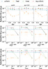Fig. 6. Trends of the KS test p value for the Πopt-versus-νpS limiting envelope, for the PL-distributed parameter space reported in Table 2. We report the KS trends as a function of Δp (top panels), rmin (middle panels), and ${\gamma }_{\mathrm{cut}}^{\min .\mathrm{ratio}}$ (bottom panels). The left, middle, and right columns refer to the selected values of q, equal to 0, 1, and –1.5, respectively. The dashed horizontal lines mark the 0.05 p-value.

We notice that consistently with the HSPs IXPE trends, the RoboPol Π_opt-versus-ν_p^S limiting envelope rules out the f_γcut = fixed PDF, and disfavor values of ${\gamma }_{\mathrm{cut}}^{\min .\mathrm{ratio}}⪆0.1$, for all the f_γcut PDFs, and values of r_min ⪆ 0.1 for the linearf_γcut. Anyhow, the Π_opt-versus-ν_p^S limiting envelope does not constrain the dispersion on Δ_p. The reason for this behavior stems from the fact that the observed RoboPol Π_opt-versus-ν_p^S envelope depends mostly on the ‘distance’ between the optical frequency and ν_p^S, and in particular on the modulation of N_ν^eff, that is, the polarization factor κ_ν^eff below ν_p^S. This effect is shown in Figures 7 and 8. In Figure 7 we plot the trial-averaged trends for N_ν^eff and for the polarization factor, κ_ν^eff for the PL scenario with f_pc = 𝒰[1.5, 2.5], q = −1.0, r_min = 0.1, and f_γcut = log-uniform. The different values of ${\gamma }_{\mathrm{cut}}^{\min .\mathrm{ratio}}$ are reported in the panel title, and the dashed vertical line marks the reference value for the optical frequency. We notice how increasing ${\gamma }_{\mathrm{cut}}^{\min .\mathrm{ratio}}$ from 0.1 to 0.9, the optical excursion across the ν_p range, of both N_ν^eff and κ_ν^eff, decreases. This leads to a different trend in the Π_opt-versus-ν_p^S plane, as shown in Figure 8, where we notice the increase of ${\gamma }_{\mathrm{cut}}^{\min .\mathrm{ratio}}$ from 0.1 to 0.9 leads to a flattening of the limiting envelope, with the KS p-value decreasing from ≈0.14, for the case of ${\gamma }_{\mathrm{cut}}^{\min .\mathrm{ratio}}=0.1$, to a p-value ≈0.015, for the case of ${\gamma }_{\mathrm{cut}}^{\min .\mathrm{ratio}}=0.9$. Finally, in Figure 9 we plot the best runs for f_γcut = uniform (top panels), f_γcut = log-uniform (middle panels), and f_γcut = linear (bottom panels). The left panels show the Π_opt-versus-ν_p^S limiting envelopes for both the MC simulations and the observed RoboPol data, the center panels show the dispersion trends of the MC optical EVPA angle, ${\sigma }_{\chi }^{\mathrm{opt}}$ vs ν_p^S, and the right panels show the IXPE HSP observed ⟨Π_ν⟩ trends compared to the MC results, extracted from the same runs used for the RoboPol panels. The decreasing trend of the optical EVPA angle dispersion has the same root as the Π_opt-versus-ν_p^S. i.e. the modulation of N_ν^eff below ν_p^S. For lower values of ν_p^S, the optical N_ν^eff decreases; hence, the dispersion on the optical EVPA angle increases.

Fig. 7. Trial-averaged trends for Nνeff and for the polarization factor, κνeff, for the PL scenario with fpc = 𝒰[1.5, 2.5], q = −1.0, rmin = 0.1, and fγcut = log-uniform. The different values of ${\gamma }_{\mathrm{cut}}^{\min .\mathrm{ratio}}$ are reported in the panel title, and the dashed vertical line marks the reference value for the optical frequency.

Fig. 8. MC Πopt-versus-νpS trend, compared to the RoboPol observed one, for the same MC run configuration as reported in Figure 7. The panels from top to bottom show the trend for increasing values of ${\gamma }_{\mathrm{cut}}^{\min .\mathrm{ratio}}$, from ${\gamma }_{\mathrm{cut}}^{\min .\mathrm{ratio}}=0.01$ (top panel) to ${\gamma }_{\mathrm{cut}}^{\min .\mathrm{ratio}}=0.9$ (bottom panels). The Πopt trend flattens for larger values of ${\gamma }_{\mathrm{cut}}^{\min .\mathrm{ratio}}$, with the KS p-value decreasing from ≈0.14, for the case of ${\gamma }_{\mathrm{cut}}^{\min .\mathrm{ratio}}=0.1$, to a p-value ≈ 0.015, for the case of ${\gamma }_{\mathrm{cut}}^{\min .\mathrm{ratio}}=0.9$.

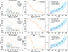Fig. 9. Best runs for fγcut = uniform (top panels), fγcut = log-uniform (middle panels), and fγcut = linear (bottom panels). The left panels show the Πopt-versus-νpS limiting envelopes for both the MC simulations and the observed RoboPol data, the center panels show the trends of the MC-averaged dispersion of the MC optical EVPA angle vs νpS, and in the right panels, the IXPE HPS observed trends compared to the MC results extracted from the same runs used for the RoboPol panels.

5.3. Phenomenology constraint on the MC parameter space

The two tests against IXPE and RoboPol data have provided an interesting constraint on the MC parameter space. We define our best sample by selecting runs resulting in a RoboPol KS p-value >  0.1, and a 20% maximal relative difference between the IXPE and MC for both the a_mm − o and a_o − X. The selection reduces the volume of the parameter space, from 780 (for the total MC volume) to 79, for the best selection volume. In Figure 11 we show the statistical outcome of the selection. In the top panels, we report the Δ_p-versus-${\gamma }_{\mathrm{cut}}^{\min .\mathrm{ratio}}$, and in the bottom panels the Δ_p-versus-r_min parameter space. The three columns refer to the selected f_γcut PDF. The blue crosses mark the total MC parameter space, and the filled circles the best sample parameter space. The color scale marks the ratio of the volume of best parameter space, at the coordinate reported on the x and y axes, to the total MC parameter space; both the volume sizes refer to the given f_γcut PDF. The plots confirm the results discussed in the previous section, i.e., the observed and combined RoboPol/IXPE phenomenology constrain Δ_p ⪆ 0.6, and ${\gamma }_{\mathrm{cut}}^{\min .\mathrm{ratio}}⪅0.1$. The log-uniformf_γcut PDF covers a larger volume of the parameter space, and reaches the peak value of the fractional acceptance, at almost 0.05. We find it quite promising that by only imposing the MC calibration condition of Π_opt ≈ 0.045, for HSP sources, our model was able to reproduce simultaneously both the IXPE and RoboPol observed phenomenology. Finally, we test our MC-predicted Π_ν trends against the data of Mrk 421, showing pronounced chromaticity in Π_ν. To this end, we restrict the ν_p^S bin to [10¹⁶, 10¹⁸] Hz (consistent with the source SED) and select the runs that best match the observed values of a_mm − o and a_o − X, ranking them by the χ² computed from each run’s median (0.5-quantile) predictions. In Figure 10 we show the top-ranked runs for f_γcut = uniform (top panel), log-uniform (middle panel), and linear (bottom panel). The MC Π_ν trends reproduce the observed chromaticity of Mrk 421 with good accuracy. This contrasts with Liodakis et al. (2022), who argued that multi-zone models can reproduce only a mild level of chromaticity in Π_ν.

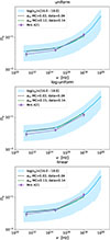Fig. 10. Πν trends for the top-ranked MC runs tested against the observed data of Mrk 421 for the case of fγcut = uniform (top panel), fγcut = log-uniform (middle panel), and fγcut = linear (bottom panel).

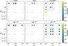Fig. 11. Statistical outcome of the PL-distributed MC parameter space selection. The Δp-versus-${\gamma }_{\mathrm{cut}}^{\min .\mathrm{ratio}}$ parameter space is shown in the top panels, whilst the bottom panels show the Δp-versus-rmin parameter space. The three columns refer to the selected fγcut PDF. The blue crosses mark the total MC parameter space, and the filled circles the best sample parameter space. The color scale marks the ratio of the volume of best parameter space, at the coordinate reported on the x and y axes, to the total MC parameter space; both volume sizes refer to the given fγcut PDF. The red boxes mark the parameter space where the MC-averaged 1-σ dispersion of the X-ray EVPA is < 25°.

6. Discussion and conclusions

We have presented an analysis of the multiwavelength pattern in the Π_ν of blazars, based on a comprehensive Monte Carlo framework modeling multi-zone synchrotron emission, able to reproduce the energy-dependent polarization characteristics observed from millimeter to X-ray wavelengths. Our approach implements spatially resolved emitting regions, with distinct physical properties, in a purely turbulent framework, that is, we do not assume any correlation between magnetic field and cell size and/or position; we only assume a power-law distribution for the cell size, and we test different levels of correlation between the size of the cells, and cutoff in the electron distribution. This minimal approach aims to provide the most likely statistical characterization of the cell distributions, in terms of size and energy of the electrons, capable to reproduce the energy-dependent polarization patterns observed in the millimiter-to-X-ray data for IXPE HPS, and in the optical for the RoboPol dataset. Our main findings are summarized below:

• The frequency-dependent polarization fraction, Π_ν does not actually depend on the number of emitting cells contributing to a given frequency, N_ν, but on the flux-weighted average effective number $N_{\nu }^{\mathrm{eff}}$, which gives the actual contribution from each cell. This effect plays a relevant role when the size of the cells and the EED have significant dispersions. According to the distributions of the cell size, and/or of the EED parameters, the difference between N_ν and $N_{\nu }^{\mathrm{eff}}$ can be of a few orders of magnitude, with $N_{\nu }^{\mathrm{eff}}<N_{\nu }$. Hence, using the estimate of N_ν, for example, from X-ray measurements of Π_ν, leads to an underestimation of the actual number, N_c, of cells populating the region, and in the number of cells radiating at lower frequencies. This effect is significant both for the total and the best MC parameter space (see Figure B.2).

• In general, Π_ν shows a broken power-law shape, with the turnover frequency around ν_p^S. For the case of no dispersion on the low-energy index of the EED, Δ_p = 0, the low energy spectral index a_l ≈ 0, whilst it increases as Δ_p increases, up to a value of a_l ≈ 0.1 for Δ_p = 1.5. a_l results to be in general independent on q, r_min, and ${\gamma }_{\mathrm{cut}}^{\min .\mathrm{ratio}}$. The only f_γcut distribution showing a dependence on ${\gamma }_{\mathrm{cut}}^{\min .\mathrm{ratio}}$ is the log-uniform, with a_l decreasing as ${\gamma }_{\mathrm{cut}}^{\min .\mathrm{ratio}}$ increases. This is expected since $f_{{\gamma }_{\mathrm{cut}}}\propto {\gamma }_{\mathrm{cut}}^{-1}$ and the cell size is uncorrelated with γ_cut; thus, lower values of ${\gamma }_{\mathrm{cut}}^{\min .\mathrm{ratio}}$ lead to a larger dispersion in the cell flux weights at low frequencies, increasing $N_{\nu }^{\mathrm{ef}}$, with a consequent hardening in the slope of the polarization factor below ν_p^S. The high-energy slope, a_h, of the polarization fraction, unlike a_l, is independent of Δ_p, and generally also of r_min and ${\gamma }_{\mathrm{cut}}^{\min .\mathrm{ratio}}$, since the modulation of $N_{\nu }^{\mathrm{eff}}$ is mainly dictated by the cell flux contributions above ν_p, which depends on the dispersion above γ_cut.

• We have tested our MC Π_ν trends against the IXPE HPS multiwavelength datasets. We find that the observed a_mm − o index significantly constrains the dispersion on p, favoring a dispersion Δ_p ⪆ 1, and values of ${\gamma }_{\mathrm{cut}}^{\min .\mathrm{ratio}}⪅0.1$ for the log-uniform distribution. We also noticed that log-uniform distribution provides the best match with the data, and that the scenario with a fixed cutoff in the EED is ruled out. The high-energy index, a_o − X, provides a lower constraining power, anyhow, a significant tension with the data is observed for r_min ≈ 1, for the case of linearf_γcut, and for values of ${\gamma }_{\mathrm{cut}}^{\min .\mathrm{ratio}}\approx 1$, for all the f_γcut distributions.

• The result from the test of the MC Π_opt-versus-ν_p^S limiting envelope against the observed RoboPol one is consistent with the outcome of the test against the IXPE HPS multiwavelength datasets. RoboPol data rules of the scenario with a fixed cutoff in the EED. Values of ${\gamma }_{\mathrm{cut}}^{\min .\mathrm{ratio}}\gtrsim 0.1$ are disfavored for all tested f_γcut PDFs. The trend is primarily sensitive to the modulation of the effective number of emitting cells at optical frequencies, which depends on the distance between the optical band and the synchrotron peak. The observed limiting envelope between optical polarization and ν_p^S is well reproduced for models with a broad distribution of cutoff energies and a sufficiently large dispersion in the EED index p. Interestingly, we find that the same driver of the Π_opt-versus-ν_p^S leads to a similar trend for the dispersion of the MC optical EVPA angle, ${\sigma }_{\chi }^{\mathrm{opt}}$ vs ν_p^S, that is, an anticorrelation with ν_p^S, in agreement with the observed RoboPol one.

• The test of our simulations against combined IXPE and RoboPol observational data has provided a further constraint on model parameter space. By selecting MC runs that simultaneously match the RoboPol limiting envelope (KS p-value >  0.1) and reproduce the IXPE millimiter-to-optical and optical-to-X-ray polarization slopes within 20% of the observed values, the allowed parameter space (reported in Figure 11) is reduced by a factor of ten, compared to the full MC parameter space. The analysis shows that the best agreement is obtained for models with a broad dispersion in the EED index (Δ_p ≳ 0.6) and values of ${\gamma }_{\mathrm{cut}}^{\min .\mathrm{ratio}}\lesssim 0.1$ (that is, a large dispersion on γ_cut), with the log-uniformf_γcut distribution providing the best agreement.

The constraints discussed above hint to both a wide range of single-cell electron spectral indices and a broad distribution of single-cell cutoff energies to reproduce the observed S multiwavelength polarization properties of blazars. The results demonstrate that a minimal, turbulence-driven multi-zone scenario can account for the key features seen in both IXPE and RoboPol datasets. We also notice that the linear model does not provide statistical improvement compared to the log-uniform, hence, the current dataset and analysis are not able to find significant evidence for this model, which mimics statistically the magnetic reconnection scenario. Nevertheless, this scenario is not ruled out.

Our results regarding the IXPE Π_ν trends are consistent with those presented in Peirson & Romani (2019); however, we have investigated a broader parameter space and presented a quantitative prediction of the related phenomenology, validated by a test against recent observational data from millimiter to X-ray frequencies. Moreover, we notice that contrary to what is reported in Liodakis et al. (2022), the multi-zone scenario is capable of reproducing the observed chromaticity of the Π_ν trends. We stress that our model does not test the presence or not of a shock, and that the investigation on the dispersion of the optical EVPA is mostly limited to the multi-zone scenario, with any implication on observed systematic rotations at different wavelengths. Hence, our analysis can fit a purely stochastic scenario or a scenario where the turbulent medium develops within the shock. In this regard, we notice how HSP objects, such as Mrk 421, have shown in their spectral shapes evidence for the coexistence of both first-order shock acceleration and stochastic acceleration (Tramacere et al. 2009, 2011). The presence of a shock is supported by recent population studies of IXPE results (Chen et al. 2024; Capecchiacci et al. 2025) providing an important observational constraint: they report EVPA–jet alignment in X-rays with a dispersion on the order of 20°(except for the larger rotations seen in Mrk 421 (Di Gesu et al. 2023)). If the EVPA–jet stable alignment reflects shock acceleration with in-shock turbulence, the MC EVPA should exhibit low dispersion, particularly in X-rays, in agreement with the IXPE results. For this purpose, in Figure 11 we marked with red boxes the points in our MC best parameter space that yield, on average, a 1-σ dispersion of the X-ray EVPA below 25°. This selection restricts the best parameter space to f_γcut distributed uniformly or log-uniformly, with Δ_p = 1.5. In particular, for the f_γcut = uniform case we obtain constraints r_min = 0.9 and ${\gamma }_{\mathrm{cut}}^{\min .\mathrm{ratio}}=0.1$, while for the f_γcut = emphlog-uniform case the constraints are r_min = 0.01 and ${\gamma }_{\mathrm{cut}}^{\min .\mathrm{ratio}}=0.1$. Across the MC parameter space, the MC-averaged 1-σ dispersion of the X-ray EVPA is < 40°, and roughly 75% of the best region is compatible with a dispersion < 35°. These constraints can help to clarify the turbulence structure developed in the jet, during states when jet-axis/EVPA alignment is observed, but stronger conclusions will require more comprehensive shock-plus-turbulence modeling and longer, more densely sampled X-ray polarimetric observations of the sources.

Acknowledgments

A.T. would like to thank the anonymous referee for carefully reading the manuscript and for giving constructive comments, which helped to improve the quality of the paper, and Enrico Massaro for fruitful discussions.

References

Appendix A: MC calibration stage

The calibration stage, performed for each run, calibrates N_c and ${\gamma }_{\mathrm{cut}}^{\mathrm{ref}}$, to obtain a trial-averaged optical polarization fraction, $⟨{\mathrm{\Pi }}_{\nu }^{\mathrm{opt}}⟩$, within [0.4 − 0.5]%, and a trial-averaged value of ${\nu }_p^S$ within=[0.8 − 1.2]×10¹⁷ Hz. As a reference value for the optical frequency, we use the value of 5 × 10¹⁴ Hz. The calibration stage proceeds as follows:

1. Initially, we set N_c = 1000, and we set ${\gamma }_{\mathrm{cut}}^{\mathrm{calib}}$ by a numerical sampling. In detail, we define a range of 100 ${\gamma }_{\mathrm{cut}}^{\mathrm{calib}}$ values, evenly spaced in the logarithm, in the range [10, 10⁸], and for each value we estimate the value of ν_p^S, according to the third of Eq.6, plugging the expectation values of $\overline{f_B}$, $\overline{f_{\delta }}$, and $\overline{f_p}$. The value of ${\gamma }_{\mathrm{cut}}^{\mathrm{calib}}$ resulting in the best match to ν_p^S = 1 × 10¹⁷ Hz is chosen.

2. A first 10-trial run is performed with the value of ${\gamma }_{\mathrm{cut}}^{\mathrm{calib}}$ obtained at the previous step. The resulting trials-averaged values of $⟨{\nu }_p^S⟩$ and the ⟨Π_ν^opt⟩ are tested against the reference values, within a relative tolerance of 0.02. If the difference exceeds the tolerance, the previous step is repeated updating the value of N_c according to equation 11, and the value of ${\gamma }_{\mathrm{cut}}^{\mathrm{calib}}$ is updated compensating the relative offset on $⟨{\nu }_p^S⟩$ according to the proportionality established by the third of, Eq.6.

Appendix B: N cells versus N eff

We investigate the dependence of $N_c/N_{\nu }^{\mathrm{eff}}$ for different values of q. In Figure B.1 we show the MC trends for the effective flux-averaged, $N_{\nu }^{\mathrm{eff}}$, at the reference frequencies used for the millimiter (2 × 10¹¹ Hz), optical (5 × 10¹⁴ Hz), and X-ray (1 × 10¹⁸ Hz) frequencies. The dependence of $N_c/N_{\nu }^{\mathrm{eff}}$ for difference values of q is reported in B.2, where the top panels refer to the full PL MC parameter space, and the bottom panels to the best sample parameter space. We notice how the number of N_c exceeds by at least a factor of 10 the value of $N_{\nu }^{\mathrm{eff}}$. The upper value of $N_c/N_{\nu }^{\mathrm{eff}}$ reaches up to a few thousands, for the X-ray (ν = 10¹⁸ Hz) frequency, and decrease to a few hundreds for the optical frequency (ν = 5 × 10¹⁴ Hz), and up to a few tens for millimiter frequency (ν = 2 × 10¹ Hz). The effect is larger for steeper values of q, meaning that a larger dispersion on the cell size amplifies the difference between N_c and $N_{\nu }^{\mathrm{eff}}$, due to the higher impact on the flux-weighted average effective number $N_{\nu }^{\mathrm{eff}}$.

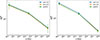Fig. B.1. The trend of the effective flux-averaged, $N_{\nu }^{\mathrm{eff}}$, at the reference frequencies used for the millimiter (2 × 1011 Hz), optical (5 × 1014 Hz), and X-ray (1 × 1018 Hz) frequencies. Different color lines mark different values of q as detailed in the legend. The left panel refers to the full PL MC parameter space, the right panel to the best sample parameter space.

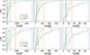Fig. B.2. The cumulative distribution function (CDF) for the ratio of the total number of cells, Nc, to the value of the effective flux-averaged, $N_{\nu }^{\mathrm{eff}}$, at the reference frequencies used for the millimiter (2 × 1011 Hz), optical (5 × 1014 Hz), and X-ray (1 × 1018 Hz) frequencies, shown respectively in the left, center, and right panels. Different color lines mark different values of q as detailed in the legend. The top panels refer to the full PL MC parameter space, the bottom panels to the best sample parameter space. The vertical dashed line marks $N_c/N_{\nu }^{\mathrm{eff}}=10$.

All Tables

All Figures

Fig. 1. Left panels: The S SED (row a), and the corresponding fractional polarization (row b) as a function of the frequency, for a power-law cutoff EED, γcut = 5 × 104, and p = [1.5, 2.0, 2.5]. The solid lines in the row b panel mark the Πνord evaluated using Eq. (1), the circles mark the δ approximation from Eq. (9) using $p_{\nu }^{(\delta )}$ from Eq. (7), and the crosses using $p_{\nu }^{(\delta )}$ from Eq. (8). The dashed lines mark the asymptotic power-law trend from Eq. (3). The relative error for the δ-approximation methods, w.r.t. the exact method (row c). In the row d panel, we report the best-fit of Πνord by means of a broken power-law function.

In the text

Fig. 2. Different colors identifying the corresponding νp bins, which are the same for all the panels. Top panels: Left column: case of identical cells (configuration ES1 in Table 1). Middle column: case of configuration ES2 in Table 1, i.e. using fγcut = log-uniform. Right column: panel, case of configuration ES3, same as ES2 but adding a flat PDF, for p : fp ∼ 𝒰[1.8, 2.8]. All the trends are reported versus ν/νp. Solid lines mark the MC 0.5 quantiles and shaded areas mark the 1-σ quantiles dispersion, for the MC trials. Row a: the trend of the ratio of ⟨Πν⟩. Row b: same as for Row 1, but for trials-averaged trends for ⟨Πν⟩/⟨Πνord⟩. Row c: trials-averaged trends for Nν (dashed lines) and $N_{\nu }^{\mathrm{eff}}$ (solid lines). Row d: trials-averaged trends for κν (dashed line) and κνeff (solid lines). Row e: SEDs for the νp bin = [1016 − 1017] Hz, the dashed vertical line shows the ν/νp value, above which not all the cells contribute to the SED flux. The dot-dashed vertical lines mark ν = νpmin, where νpmin is the SED peak value for the lowest flux cell.

In the text

Fig. 3. Summary of the polarization slope trends for the PL-distributed parameter space reported in Table 2. Each subpanel refers to the three different values of q = [0, −1.0, −1.5], as reported in the subpanel title. Top panels: Low-energy (al, left panels) and high-energy (ah, right panels) polarization slopes as a function of the dispersion in the electron energy distribution index, Δp. Middle panels: al and ah as a function of the minimum cell size ratio, rmin. Bottom panels: al and ah as a function of the minimum cutoff ratio, ${\gamma }_{\mathrm{cut}}^{\min .\mathrm{ratio}}$. Different colors correspond to the different fγcut PDF reported in the top legend.

In the text

Fig. 4. Left panel: The limiting envelope, found by RoboPol (Angelakis et al. 2016), for a large sample of γ-ray-loud blazars between νpS and both the average fractional optical polarization and its dispersion. Right panel: The Πν trend observed in by IXPE for the HPS Mrk 501, Mrk 421, PKS2155-304, 1ES0229+200, and 1ES1959+650 collected from recent IXPE multiwavelength campaigns (Liodakis et al. 2022; Di Gesu et al. 2023; Kouch et al. 2024; Middei et al. 2023).

In the text

Fig. 5. Summary of polarization slope trends for the PL-distributed parameter space reported in Table 2, for the HSP objects, selecting MC runs with (10 × 15 Hz ≤ νpS ≤ 10 × 18 Hz). Top panels: Low-energy (amm − o, left panels) and high-energy (ao − X, right panels) polarization slopes as a function of the dispersion in the electron energy distribution index, Δp. Middle panels: al and ah as a function of the minimum cell size ratio, rmin. Bottom panels: al and ah as a function of the minimum cutoff ratio, ${\gamma }_{\mathrm{cut}}^{\min .\mathrm{ratio}}$. Different colors and line styles correspond to the various PDFs parameter configurations as indicated in the legend and in the titles of the panels.

In the text

Fig. 6. Trends of the KS test p value for the Πopt-versus-νpS limiting envelope, for the PL-distributed parameter space reported in Table 2. We report the KS trends as a function of Δp (top panels), rmin (middle panels), and ${\gamma }_{\mathrm{cut}}^{\min .\mathrm{ratio}}$ (bottom panels). The left, middle, and right columns refer to the selected values of q, equal to 0, 1, and –1.5, respectively. The dashed horizontal lines mark the 0.05 p-value.

In the text

	Fig. 7. Trial-averaged trends for Nνeff and for the polarization factor, κνeff, for the PL scenario with fpc = 𝒰[1.5, 2.5], q = −1.0, rmin = 0.1, and fγcut = log-uniform. The different values of ${\gamma }_{\mathrm{cut}}^{\min .\mathrm{ratio}}$ are reported in the panel title, and the dashed vertical line marks the reference value for the optical frequency.
In the text

Fig. 8. MC Πopt-versus-νpS trend, compared to the RoboPol observed one, for the same MC run configuration as reported in Figure 7. The panels from top to bottom show the trend for increasing values of ${\gamma }_{\mathrm{cut}}^{\min .\mathrm{ratio}}$, from ${\gamma }_{\mathrm{cut}}^{\min .\mathrm{ratio}}=0.01$ (top panel) to ${\gamma }_{\mathrm{cut}}^{\min .\mathrm{ratio}}=0.9$ (bottom panels). The Πopt trend flattens for larger values of ${\gamma }_{\mathrm{cut}}^{\min .\mathrm{ratio}}$, with the KS p-value decreasing from ≈0.14, for the case of ${\gamma }_{\mathrm{cut}}^{\min .\mathrm{ratio}}=0.1$, to a p-value ≈ 0.015, for the case of ${\gamma }_{\mathrm{cut}}^{\min .\mathrm{ratio}}=0.9$.

In the text

Fig. 9. Best runs for fγcut = uniform (top panels), fγcut = log-uniform (middle panels), and fγcut = linear (bottom panels). The left panels show the Πopt-versus-νpS limiting envelopes for both the MC simulations and the observed RoboPol data, the center panels show the trends of the MC-averaged dispersion of the MC optical EVPA angle vs νpS, and in the right panels, the IXPE HPS observed trends compared to the MC results extracted from the same runs used for the RoboPol panels.

In the text

	Fig. 10. Πν trends for the top-ranked MC runs tested against the observed data of Mrk 421 for the case of fγcut = uniform (top panel), fγcut = log-uniform (middle panel), and fγcut = linear (bottom panel).
In the text

Fig. 11. Statistical outcome of the PL-distributed MC parameter space selection. The Δp-versus-${\gamma }_{\mathrm{cut}}^{\min .\mathrm{ratio}}$ parameter space is shown in the top panels, whilst the bottom panels show the Δp-versus-rmin parameter space. The three columns refer to the selected fγcut PDF. The blue crosses mark the total MC parameter space, and the filled circles the best sample parameter space. The color scale marks the ratio of the volume of best parameter space, at the coordinate reported on the x and y axes, to the total MC parameter space; both volume sizes refer to the given fγcut PDF. The red boxes mark the parameter space where the MC-averaged 1-σ dispersion of the X-ray EVPA is < 25°.

In the text

	Fig. B.1. The trend of the effective flux-averaged, $N_{\nu }^{\mathrm{eff}}$, at the reference frequencies used for the millimiter (2 × 1011 Hz), optical (5 × 1014 Hz), and X-ray (1 × 1018 Hz) frequencies. Different color lines mark different values of q as detailed in the legend. The left panel refers to the full PL MC parameter space, the right panel to the best sample parameter space.
In the text

Fig. B.2. The cumulative distribution function (CDF) for the ratio of the total number of cells, Nc, to the value of the effective flux-averaged, $N_{\nu }^{\mathrm{eff}}$, at the reference frequencies used for the millimiter (2 × 1011 Hz), optical (5 × 1014 Hz), and X-ray (1 × 1018 Hz) frequencies, shown respectively in the left, center, and right panels. Different color lines mark different values of q as detailed in the legend. The top panels refer to the full PL MC parameter space, the bottom panels to the best sample parameter space. The vertical dashed line marks $N_c/N_{\nu }^{\mathrm{eff}}=10$.

In the text

References

- Abdo, A. A., Ackermann, M., Agudo, I., et al. 2010, ApJ, 716, 30 [NASA ADS] [CrossRef] [Google Scholar]
- Angelakis, E., Hovatta, T., Blinov, D., et al. 2016, MNRAS, 463, 3365 [NASA ADS] [CrossRef] [Google Scholar]
- Blandford, R. D., & Königl, A. 1979, ApJ, 232, 34 [Google Scholar]
- Blandford, R. D., & Rees, M. J. 1978, Proceedings of the Pittsburgh Conference on BL Lac Objects (University of Pittsburgh), 328 [Google Scholar]
- Böttcher, M., Reimer, A., Sweeney, K., & Prakash, A. 2013, ApJ, 768, 54 [Google Scholar]
- Capecchiacci, S., Liodakis, I., Middei, R., et al. 2025, A&A, 703, A19 [NASA ADS] [CrossRef] [EDP Sciences] [Google Scholar]
- Chen, C.-T. J., Liodakis, I., Middei, R., et al. 2024, ApJ, 974, 50 [NASA ADS] [CrossRef] [Google Scholar]
- Di Gesu, L., Marshall, H. L., Ehlert, S. R., et al. 2023, ApJ, 949, L42 [NASA ADS] [CrossRef] [Google Scholar]
- Fasano, G., & Franceschini, A. 1987, MNRAS, 225, 155 [NASA ADS] [CrossRef] [Google Scholar]
- King, O. G., Angelakis, E., Hovatta, T., et al. 2014, MNRAS, 442, 1706 [NASA ADS] [CrossRef] [Google Scholar]
- Kirk, J. G., Rieger, F. M., & Mastichiadis, A. 2000, A&A, 333, 452 [Google Scholar]
- Kouch, P. M., Liodakis, I., Middei, R., et al. 2024, A&A, 689, A119 [NASA ADS] [CrossRef] [EDP Sciences] [Google Scholar]
- Li, X., Guo, F., Liu, Y.-H., & Li, H. 2023, ApJ, 954, L37 [NASA ADS] [Google Scholar]
- Liodakis, I., Marscher, A. P., Agudo, I., et al. 2022, Nature, 611, 677 [CrossRef] [Google Scholar]
- Marscher, A. P. 2014, ApJ, 780, 87 [Google Scholar]
- Marscher, A. P., & Jorstad, S. G. 2022, Universe, 8, 644 [NASA ADS] [CrossRef] [Google Scholar]
- Middei, R., Liodakis, I., Perri, M., et al. 2023, ApJ, 942, L10 [NASA ADS] [CrossRef] [Google Scholar]
- Pavlidou, V., Blinov, D., Angelakis, E., et al. 2014, MNRAS, 442, 1693 [NASA ADS] [CrossRef] [Google Scholar]
- Peacock, J. A. 1983, MNRAS, 202, 615 [NASA ADS] [Google Scholar]
- Peirson, A. L., & Romani, R. W. 2019, ApJ, 885, 76 [NASA ADS] [CrossRef] [Google Scholar]
- Press, W. H., Teukolsky, S. A., Vetterling, W. T., & Flannery, B. P. 2007, Numerical Recipes: The Art of Scientific Computing, 3rd edn. (Cambridge University Press), see Section 14.8 [Google Scholar]
- Rybicki, G. B., & Lightman, A. P. 1986, Radiative Processes in Astrophysics (Wiley-VCH), 400 [Google Scholar]
- Shook-Sa, B. E., & Hudgens, M. G. 2022, Biometrics, 78, 388 [Google Scholar]
- Sironi, L., Giannios, D., & Petropoulou, M. 2016, MNRAS, 462, 48 [NASA ADS] [CrossRef] [Google Scholar]
- Stein, C. 1945, AnnMathStat, 16, 243 [Google Scholar]
- Tramacere, A. 2020, Astrophysics Source Code Library [record ascl:2009.001] [Google Scholar]
- Tramacere, A., Giommi, P., Perri, M., Verrecchia, F., & Tosti, G. 2009, A&A, 501, 879 [NASA ADS] [CrossRef] [EDP Sciences] [Google Scholar]
- Tramacere, A., Massaro, E., & Taylor, A. M. 2011, ApJ, 739, 66 [Google Scholar]
- Urry, C. M., & Padovani, P. 1995, PASP, 107, 803 [NASA ADS] [CrossRef] [Google Scholar]
- Weisskopf, M. C., Ramsey, B., O’Dell, S., et al. 2022, JATIS, 8, 026002 [NASA ADS] [Google Scholar]
- Westfold, K. C. 1959, ApJ, 130, 241 [Google Scholar]
- Wübbeler, G., Harris, P. M., Cox, M. G., & Elster, C. 2010, Metrologia, 47, 317 [Google Scholar]