| Issue |
A&A
Volume 705, January 2026
|
|
|---|---|---|
| Article Number | A114 | |
| Number of page(s) | 27 | |
| Section | Extragalactic astronomy | |
| DOI | https://doi.org/10.1051/0004-6361/202553820 | |
| Published online | 12 January 2026 | |
Constraints on the z ∼ 6−13 intergalactic medium from JWST spectroscopy of Lyman-alpha damping wings in galaxies
1
Cosmic Dawn Center (DAWN)
2
Niels Bohr Institute, University of Copenhagen Jagtvej 128 2200 Copenhagen N, Denmark
3
Steward Observatory, University of Arizona 933 N Cherry Ave Tucson AZ 85721, USA
4
Department of Astronomy, University of California Berkeley CA 94720, USA
★ Corresponding author: This email address is being protected from spambots. You need JavaScript enabled to view it.
Received:
20
January
2025
Accepted:
6
November
2025
Abstract
Context. JWST provides a unique dataset for studying the earliest stages of reionisation at z > 9, promising insights into the first galaxies. Many JWST/NIRSpec prism spectra of z > 5 galaxies have revealed smooth Lyman-alpha breaks, implying damping wing scattering by neutral hydrogen.
Aims. We investigate what current prism spectra imply about the intergalactic medium (IGM) at z > 6 and how best to use NIRSpec spectra to recover IGM properties. We use a sample of 99 z ∼ 5.5 − 13 galaxies with high S/N prism spectra in the public archive, including 12 at z > 10.
Methods. We analyse these spectra using damping wing sightlines from inhomogeneous reionising IGM simulations, mapping between the distance of a source from the neutral IGM and the average IGM neutral fraction. We marginalise over absorption by local neutral hydrogen around the galaxies and Lyman-alpha emission.
Results. We observe a decline in the median and variance of flux around the Lyα break with increasing redshift, consistent with an increasingly neutral IGM, as ionized regions become smaller and rarer. At z ≳ 9 the spectra become consistent with an almost fully neutral IGM. We find S/N > 15 per pixel is required to robustly estimate IGM properties from prism spectra. We fit a sub-sample of high S/N spectra and infer mean IGM neutral fractions of x̄HI = 0.33−0.27+0.18, 0.64−0.23+0.17 (> 0.70 excluding GNz11) at z ≈ 6.5, 9.3. We also investigate local HI absorption, finding a median column density of log10NH I ≈ 1020.8 cm−2, comparable to z ∼ 3 Lyman-break galaxies, with no significant redshift evolution z ≳ 5.5. We find galaxies showing the highest column density absorption are more likely to be in close associations of sources (≲500 pkpc), implying absorption is enhanced in massive dark matter halos. Future deep prism and grating spectroscopy of z > 9 sources will provide tighter constraints on the earliest stages of reionisation, key for understanding the onset of star formation.
Key words: galaxies: high-redshift / intergalactic medium / dark ages, reionization, first stars
© The Authors 2026
 Open Access article, published by EDP Sciences, under the terms of the Creative Commons Attribution License (https://creativecommons.org/licenses/by/4.0), which permits unrestricted use, distribution, and reproduction in any medium, provided the original work is properly cited.
This article is published in open access under the Subscribe to Open model. This email address is being protected from spambots. You need JavaScript enabled to view it. to support open access publication.
1. Introduction
Understanding the reionisation of intergalactic hydrogen in the early Universe has long been a frontier in astronomy. In the last two decades significant progress has been made in constraining the end stages of reionisation, with multiple independent observations demonstrating reionisation was complete by z ∼ 5.3 − 6 and ongoing at z ∼ 7 − 8 (e.g. Stark et al. 2010; Ouchi et al. 2017; Planck Collaboration VI 2020; Mason et al. 2018b; Davies et al. 2018; Qin et al. 2025). However, until the launch of JWST, we had no observational constraints on the earliest stages of reionisation at z ≳ 8. Constraints on the early intergalactic medium (IGM) promise crucial information about the onset of star formation and the higher-than-expected UV luminosity density detected by JWST at z > 9 (e.g. Castellano et al. 2022; Naidu et al. 2022; Adams et al. 2023; Donnan et al. 2023; Harikane et al. 2023; Finkelstein et al. 2022), as the collective ionizing output of galaxies below even JWST’s detection limits will be felt in the IGM.
JWST finally provides the ability to chart the earliest stages of reionisation through measurements of the Lyman-alpha (Lyα) damping wing, due to scattering by neutral hydrogen in the IGM, in z > 8 galaxies. The damping wing feature results in smooth absorption up to several thousand kilometres per second redward of Lyα in the spectra of high redshift sources (e.g. Miralda-Escude 1998). The strength of absorption depends on the density and spatial distribution of neutral hydrogen along the line of sight and thus can be used to constrain the properties of the high-redshift IGM. Before the launch of JWST, Lyα damping wings had been observed in just four bright quasars at z ∼ 7 − 7.5 (Mortlock et al. 2011; Bañados et al. 2018; Wang et al. 2020; Yang et al. 2020). In galaxies, which are fainter but orders of magnitude more numerous than quasars, the integrated impact of the damping wing had been detected as a decrease in the equivalent width distribution of galaxies’ Lyα emission (e.g. Stark et al. 2010; Pentericci et al. 2014; Mason et al. 2019; Jung et al. 2020; Bolan et al. 2022) and the decline in Lyα-emitter luminosity functions (e.g. Ouchi et al. 2017; Hu et al. 2019; Morales et al. 2021; Umeda et al. 2025b) at z ≳ 6.
The spectral sensitivity of JWST/NIRSpec (Jakobsen et al. 2022) has enabled the first detection of the UV continuum for typical star-forming galaxies at z > 5 and thus direct observations of the IGM damping wing. Excitingly, early JWST results have revealed many z > 9 galaxies show strong damping wing features in their spectra (e.g. Curtis-Lake et al. 2023; Umeda et al. 2024; Heintz et al. 2024b), and a continued decline in the Lyα equivalent width distribution at z ≳ 8 (Nakane et al. 2024; Tang et al. 2024c; Jones et al. 2025; Kageura et al. 2025), implying we are finally detecting galaxies in an almost fully neutral IGM. However, JWST spectroscopy has also provided hints of early ionized bubbles via surprising detections of Lyα from galaxies at z ≈ 11 and z ≈ 13 (Bunker et al. 2023; Witstok et al. 2025). Placing these detections in context requires a large census of z ≳ 9 spectra. Current and future spectroscopic surveys with JWST provide the potential to precisely chart the earliest stages of reionisation via both the decline in Lyα emission and the impact of IGM damping on the UV continuum redward of Lyα.
However, JWST spectra also present unique challenges for inferring properties of the IGM from the UV continuum. The most efficient spectroscopic mode is the NIRSpec prism. The low spectral resolution of the prism around 1 μm (R ∼ 40) means the damping wing appears in only ∼5 pixels. Moderate Lyman-alpha emission (Lyα, EW ≲50 Å) can be spread across these pixels and confused with a high continuum flux (Keating et al. 2024a; Chen et al. 2024; Jones et al. 2024; Park et al. 2025), in addition to NV P-Cygni stellar wind lines, which may be present in sources with ≲10 Myr massive stars (e.g. Chisholm et al. 2019), and interstellar absorption lines. Furthermore, galaxies at all redshifts are commonly observed with absorption around Lyα due to dense neutral hydrogen in the ISM and CGM, and proximate absorbers along the line of sight, (e.g. Shapley et al. 2003; Reddy et al. 2016; Hu et al. 2023; Heintz et al. 2025). These features also change the shape of the UV continuum, though, as we show below, with a different wavelength dependence than the neutral IGM, but may be hard to distinguish from the IGM with low resolution, low S/N spectra.
Umeda et al. (2024) have presented the most comprehensive study of galaxy damping wings to date, fitting the spectra of 27 spectroscopically confirmed z > 7 galaxies, including the impact of Lyα emission and neutral hydrogen (HI) in the host galaxies in the spectra, to infer the IGM neutral fraction  at z ∼ 7 − 13, finding evidence for an increasing neutral fraction with redshift. However, to fit the IGM damping wing from galaxy spectra, this, and most previous works with JWST, have assumed a simple analytical model for the Lyα transmission that approximates the IGM as ionized within the galaxies’ host bubble and uniform beyond the bubble with neutral fraction
  (Miralda-Escude 1998). While this model reproduces the median IGM transmission in realistic IGM simulations at fixed
  (Keating et al. 2024a), using it to fit individual sources can bias inferred
  , as it overestimates the contribution of neutral gas at large distances (Mesinger & Furlanetto 2008). The damping wing optical depth most strongly depends on the distance of a galaxy to the first neutral patch; thus accurate
  inferences require a realistic mapping between the ionized bubble size distribution as a function of redshift and
  . In this work, we present an analysis of galaxy damping wings using sightlines from realistic inhomogeneous IGM simulations that can capture this mapping.
In this paper we seek to understand what current NIRSpec prism spectra imply about the IGM at z ≳ 6 and how best to use NIRSpec galaxy continuum spectra to robustly recover IGM properties. We use a sample of 99 z > 5.5 galaxies, including 12 at z > 10, to explore the redshift evolution of the Lyα break. We find a decrease in both the flux and variance of the strength of the break, which we interpret as being most likely due to an increasingly neutral IGM, as large ionized regions become smaller and rarer. We describe an approach for fitting the UV continuum using damping wing sightlines from realistic IGM simulations to forward-model galaxy spectra, accounting for the inhomogeneous nature of the reionising IGM and marginalising over galaxies’ Lyα emission and local absorption systems, to infer constraints on galaxies’ distances from neutral gas and the mean neutral fraction  .
.
This paper is structured as follows: In Section 2 we present our method for modelling the Lyα damping wing optical depth, due to both neutral IGM and local absorbers. We describe our observational sample, obtained from public JWST Cycle 1 and 2 NIRSpec spectra, in Section 3, and our spectral fitting approach in Section 4. We present the evolution of the spectra and our fits to these spectra in Section 5. We discuss our results in the context of the reionisation process and local absorption systems in Section 6, and we present our conclusions in Section 7.
We use the best-fit cosmological parameters from Planck 2018 data (TT,TE,EE+lowE+lensing+BAO from Planck Collaboration VI 2020). All distances are comoving unless specified otherwise.
2. Modelling the Lyman-alpha damping wing
Following Mesinger et al. (2015) and Mason et al. (2018b), we model the contribution of diffuse neutral gas in the IGM (Section 2.1), and the dense HI in the surroundings of galaxies (Section 2.2) separately, i.e. τα = τIGM + τDLA, as we describe below.
2.1. Optical depth through the reionising IGM
We first describe the general properties of the Lyα optical depth due to the inhomogeneous distribution of neutral hydrogen in the IGM along the line of sight expected during reionisation. In Section 2.1.1 we then describe the simulations we used to model the distribution of neutral hydrogen in the reionising IGM.
For each sightline to a galaxy, the optical depth due to diffuse neutral hydrogen in the IGM can be approximated by the integral over the damping wing component of the optical depth in every neutral patch along the sightline:
 (1)
(1)
where Db is the distance of the galaxy from the edge of its host ionized bubble along the line of sight. We set Dmax = 1.6 cGpc, wrapping around our simulation cubes as necessary (see Section 2.1.1) assuming periodic boundaries (the optical depth converges after ∼200 cMpc, e.g. Mesinger & Furlanetto 2008). The contribution to the optical depth from each neutral patch i along the line of sight is given by (e.g. Miralda-Escude 1998)
![Mathematical equation: $$ \begin{aligned} d\tau _{igm ,i}(z)&= 6.43\times 10^{-9} x_{HI ,i} \tau _\mathrm{GP} (z) \nonumber \\&\times \left[ I\left(\frac{1+z_{\mathrm{begin} ,i}}{1+z}\right) - I\left(\frac{1+z_{\mathrm{end} ,i}}{1+z}\right) \right], \end{aligned} $$](/articles/aa/full_html/2026/01/aa53820-25/aa53820-25-eq10.gif) (2)
(2)
where  is the neutral fraction in each patch (we assume
  ), and
 ![Mathematical equation: $ \tau_{\mathrm{GP}}(z) = \pi e^2 f_\alpha \overline{n}_{\mathrm{H}}(z)/[m_{\mathrm{e}} c H(z)] $](/articles/aa/full_html/2026/01/aa53820-25/aa53820-25-eq13.gif) is the Gunn & Peterson (1965) optical depth, where e is the electron/proton charge, fα = 0.416 is the Lyα oscillator strength, me is the electron mass, and
is the Gunn & Peterson (1965) optical depth, where e is the electron/proton charge, fα = 0.416 is the Lyα oscillator strength, me is the electron mass, and  is the mean hydrogen number density. Here, 1 + z = (1 + zg)λemit/λLyα, where zg is the redshift of the galaxy and λLyα is the rest-frame wavelength of Lyα (1216 Å). The function I(x), defined below, is evaluated at zbegin, i ≈ zg − cDb, i/H(z), the redshift of the beginning of a neutral patch a comoving distance Db, i from the galaxy, and zend, i, the redshift of the end of the neutral patch, and finally,
 (3)
(3)
We assume gas inside ionized regions is optically thick to Lyα photons at resonance (i.e. τ(λemit ≤ λLyα)→∞), truncating the blue side of Lyα (Mason & Gronke 2020), as expected given the opacity in the Lyα forest at z ≳ 6 (Bosman et al. 2022). Gravitational infall of the IGM will shift this truncation redward of the Lyα resonant wavelength (e.g. Santos 2004; Dijkstra et al. 2007), which we also include (see Section 4).
We gain two important insights by considering the limit zend ≪ zbegin (i.e. a single ionized patch out to Db from the source, followed by neutral gas up to a distance Dmax ≫ Db): (1) the IGM optical depth is sensitive to neutral gas within ∼100 cMpc, i.e. very large distances, (2) because I(x) increases very steeply with x, neutral gas closest to the galaxy has the highest contribution to the damping wing. (2) has important consequences for reionisation inferences.
In particular, it implies that individual galaxy spectra mostly tell us about distance of a galaxy to the neutral IGM, Db, and are much less sensitive to the global neutral fraction,  (see Appendix A; Mesinger & Furlanetto 2008; Chen 2024; Keating et al. 2024b). Simulations predict a wide distribution of bubble sizes at fixed
  , and galaxies sit in a variety of positions within bubbles, resulting in significant variance in Db and thus damping wing profiles (see Figure 1, Lu et al. 2024). In Figure 2 we plot the distribution of Db as a function of
  from the simulations we use in this work (see Section 2.1.1 below), clearly demonstrating the broad distribution. The median Db tracks the mean bubble radius1 (as estimated using the mean free path method, Lu et al. 2024), but the large variance in Db, in addition to measurement uncertainties on Db from fitting damping wings (e.g. σ(log10Db)≳0.5 − 0.7 dex when fitting NIRSpec prism spectra, see discussion in Section 6.3), means a single galaxy cannot precisely constrain the mean bubble size and thus
  .
.
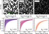 |
Fig. 1. Top panels: Example 300 cMpc × 300 cMpc slices of the ionization field (white patches show ionized gas, black neutral gas) in our (1.6 cGpc)3 simulations at |
![Mathematical equation: $ \overline{x}_{{\small { {\text{HI}}}}}=[0.5,0.7,0.9] $](/articles/aa/full_html/2026/01/aa53820-25/aa53820-25-eq20.gif)


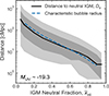 |
Fig. 2. Median, 68% and 95% range of distances of MUV ∼ −19.3 galaxies (the median in our sample) to the neutral IGM, Db as a function of |

Accurately inferring  from damping wing observations therefore requires observations of tens of galaxies at a given redshift (see discussion in Section 6.3) to recover a distribution of Db (or damping wing optical depths), and a mapping between these distribution and
  . Such a mapping is possible using damping wing sightlines or bubble size distributions from simulations run on grids of fixed
  , which allow us to statistically link the observed distribution of Lyα transmission properties to
  . For single sources, even with very high S/N spectroscopy, the resulting uncertainty in
  due to the broad distribution of Db at fixed
  can be ∼0.3 (see e.g. Greig et al. 2017; Davies et al. 2018; Wang et al. 2020; Yang et al. 2020, for damping wing analyses of z > 7 quasars, and Kist et al. 2025b for an extensive discussion of this sightline variance). Combining many sources thus provides tighter constraints on
  (e.g. considering the evolution of the Lyα EW distribution in z > 6 galaxies, see Mesinger et al. 2015; Mason et al. 2018b; Bolan et al. 2022; Tang et al. 2024c).
Most analyses of Lyα damping wings in galaxies observed by JWST to date have assumed a uniform IGM with a volume-averaged neutral fraction  , and, but not always, with a single ionized bubble around each galaxy (following e.g. Miralda-Escude 1998). However, because the damping wing is more sensitive to Db than to
  , not only does this neglect the sightline variance, this approach can lead to significant biases in the inferred
  (discussed in detail by Mesinger & Furlanetto 2008). In particular, the uniform IGM approximation can underestimate the damping wing for galaxies in small bubbles during the late stages of reionisation and overestimate it during earlier stages (see Appendix A). Relatively accurate estimates of Db can be obtained assuming a fully neutral IGM beyond the first bubble (e.g. Mason & Gronke 2020; Hayes & Scarlata 2023), but still require a mapping from the inferred distribution of Db to
  (e.g. Tang et al. 2024c). In this work we analyse JWST spectra using sightlines from realistic, inhomogeneous IGM simulations from Lu et al. (2024), described in Section 2.1.1, allowing us to map between inferred damping wings parameterised by Db, and the IGM neutral fraction
  . Here, we consider a single reionisation morphology model, but we do not expect this to significantly impact our
  inference – as demonstrated by Sobacchi & Mesinger (2015), Greig et al. (2017, 2019), Mason et al. (2018a), the Lyα damping wing transmission is fairly insensitive to the reionisation morphology when considering > L★ galaxies (as we do for our study due to their higher S/N spectra) which are likely to be in the largest ionized regions in all reionisation models (Lu et al. 2024), and when considering redshift bins broader than the typical scales of bubbles (Δz ≳ 0.1, as will be the case with our study) which smooths out information about the reionisation morphology (Sobacchi & Mesinger 2015). In an upcoming work we will discuss cases where differences in the reionisation morphology could be distinguished (i.e. for UV-faint galaxies observed in narrower redshift windows).
In Figure 3 we show mock spectra, convolved to the resolution of the NIRSpec prism and G140M gratings, showing the impact of the neutral IGM. Here we have taken a template high resolution spectrum at z ∼ 10 (see Section 4), adding a Gaussian Lyα emission line with EW = 100 Å, FWHM = 200 km s−1 and velocity offset from systemic Δv = 200 km s−1. We apply IGM damping wings using Equation 1, assuming a single ionized region in a fully neutral IGM. Figure 3 shows large (> 1 dex) changes in the distance to neutral IGM, Db, can be clearly distinguished. However, distinguishing Db ≲ 3 cMpc is challenging in the prism, whereas these can be distinguished with G140M, especially if Lyα emission is present. This is because the gradient of the damping wing is steepest closest to line center, making deep constraints on Lyα emission most important for measuring Db in the early stages of reionisation when bubbles are expected to have R ≲ 10 cMpc (Lu et al. 2024). We discuss prospects for constraining the damping wing signal with grating spectra in Section 6.3. Overall, we see the NIRSpec prism provides an efficient, though relatively blunt, tool for constraining IGM properties.
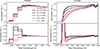 |
Fig. 3. Mock spectra at z = 10 demonstrating the impact of the distance from neutral IGM, Db. Left (right) panels show the spectrum convolved to the resolution of the NIRSpec prism (G140M grating). The grey line shows the spectrum in an almost fully ionized IGM (i.e. Lyα is attenuated only blueward of resonance by the Gunn & Peterson (1965) optical depth). Coloured lines show the spectrum if the galaxy is a distance Db = 1 − 100 cMpc from the neutral IGM. The top panels show a case with no Lyα emission, while the bottom panels show the same spectrum including Lyα emission with pre-IGM EW = 100 Å, FWHM = 200 km s−1 and Δv = 200 km s−1, where weak Lyα due to the smallest Db can only be clearly identified in the G140M spectrum. |
2.1.1. Reionisation simulations
To obtain realistic IGM damping wings, we used semi-numerical reionisation simulations by Lu et al. (2024), which are optimised for comparison to JWST observations, and refer the reader there for full details. The simulations were created using the semi-numerical code 21cmFAST-v2 (Mesinger & Furlanetto 2007; Sobacchi & Mesinger 2014; Mesinger et al. 2016). 21cmFAST-v2 generates IGM properties from a 3D density field, flagging cells as ionized when the rate of ionizations exceeds the rate of recombinations. The ionization rate is set by the collapsed matter fraction in a cell multiplied by an ionization parameter.
We created a grid of simulation cubes, using the same initial conditions, at fixed redshifts z ∼ 6 − 16, with Δz = 1, which are each (1.6 cGpc)3 volume – sufficient to sample 100s of MUV ∼ −22 galaxies, with ∼1 cMpc resolution in the IGM. For each cube, we used a halo-filtering approach in Extended Press-Schechter theory (Sheth et al. 2001) to generate a halo catalog from the associated density field (see Mesinger & Furlanetto (2007) for a full description of the method) and assign UV luminosities to halos based on the Mason et al. (2015) luminosity function model, which successfully reproduces observations over z ∼ 0 − 10 (see Lu et al. 2024, for a comparison of the simulated LFs and observations), enabling us to account for the expected large-scale environment of the observed galaxies. We note, while this model does not match z > 10 JWST LFs well (Mason et al. 2023), as shown by Whitler et al. (2020), Lu et al. (2024) the exact environment of galaxies as a function of UV luminosity is less important than the average neutral fraction in determining Lyα visibility, so this should not significantly impact our results. We include 0.5 mag scatter in the halo mass – UV luminosity mapping to include the impact of stochastic star formation (e.g. Ren et al. 2019; Mason et al. 2023; Gelli et al. 2024), but note this has only a small impact on galaxies’ Lyα transmission (Whitler et al. 2020). We vary the ionization parameter to produce IGM cubes from the density field at neutral fractions  , with spacing
  , from which we sample IGM damping wings to every halo to generate a catalogue of damping wings as a function of redshift,
  , Db and MUV.
In Figure 1 we show example slices from our IGM cubes at z = 8, showing  , and the corresponding median and 68% and 95% ranges of IGM damping wings. Figure 1 demonstrates there is large sightline variance in Lyα transmission due to the broad bubble size distributions, especially during the mid-stages of reionisation (see also, e.g. Mesinger & Furlanetto 2008; Mason et al. 2018a; Keating et al. 2024a), and thus the importance of using simulations to map from damping wing observations to
  estimates. In Section 6.3, we demonstrate we require ∼20 sightlines, i.e. galaxies, per redshift bin to accurately recover
  .
.
2.2. Optical depth from local absorbers
In addition to the Lyα damping wing from the IGM, sources can also experience Lyα damping absorption from dense HI gas on local (< 1 pMpc) scales. Spectroscopic studies at z ∼ 0 − 4 have shown that roughly half of Lyman-break galaxies show absorption around Lyα, often in addition to Lyα emission (Shapley et al. 2003; Heckman et al. 2011; Rivera-Thorsen et al. 2015; Reddy et al. 2016; Pahl et al. 2020; Hu et al. 2023; Begley et al. 2024), which has recently been extended to z > 5 with JWST (e.g. Chen et al. 2024; Heintz et al. 2024b, 2025; Hainline et al. 2024). These results imply neutral gas in the ISM and/or CGM with column densities NH I ≳ 1020 cm−2, i.e. damped Lyα absorbers (DLAs), though with a non-uniform covering fraction (e.g. Heckman et al. 2011; Reddy et al. 2016). Proximate absorbers along the line of sight may also provide additional opacity (e.g. Davies et al. 2025).
A key question is to what extent this local absorption affects our ability to estimate the impact of the IGM at z ≳ 6. McQuinn et al. (2008) and Lidz et al. (2021) have discussed this in the context of measuring IGM damping wings in gamma ray burst (GRB) spectra and demonstrated the absorption profiles due to the IGM and local gas are significantly different. The optical depth from local HI gas can be approximated by:
 (4)
(4)
where we use the approximation for the Lyα optical depth σα given by Tasitsiomi (2006). As the damping wings are set by natural line broadening, the temperature, T, of the absorbing gas has negligible impact on the optical depth, so we set T = 104 K.
The Lorentzian wing of the Lyα optical depth (e.g. see Dijkstra 2014, for a review) implies τDLA ∼ 1/(Δλ)2, while the IGM damping wing, being an integral over a much longer path length, follows a shallower profile, τIGM ∼ 1/(Δλ). This means the impact of the IGM and DLAs can be distinguished in the UV continuum.
We demonstrate this in Figure 4 where we show Lyα transmission profiles for a fully neutral IGM versus local absorption through various column densities NH I, and the combination of both local absorption and the neutral IGM for both grating and prism resolution. The steep local HI absorption profile relative to the IGM damping wing is clearly seen for NH I ≲1021 cm−2 where more flux is reduced at linecenter. At fixed NH I, the addition of neutral IGM suppresses flux at longer wavelengths. Only for extremely high column densities, NH I ≳ 1022 cm−2 does the DLA damping wing start to dominate over the IGM damping wing. Recent JWST observations have presented evidence of DLAs reaching NH I ≈ 1022.0−22.5 around some sources (Heintz et al. 2024b; Chen et al. 2024; D’Eugenio et al. 2024), but as we show in Section 6.2, this is likely a tail of the distribution, and the majority of z ≳ 5 sources have lower inferred column densities. In Appendix B we show mock spectra for both the prism and G140M resolution grating, finding that, given sufficient S/N, the IGM can be distinguished from local absorption. In Figure 4 we also show how the damping wing for a fully neutral IGM evolves with redshift, becoming similar in strength to a NH I ≳ 1021−21.5 cm−2 DLA at z ∼ 6 − 14.
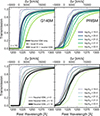 |
Fig. 4. Transmission (e−τ) as a function of wavelength around Lyα due to the neutral IGM and local absorbers for high resolution (R ≳ 1000, left panels) and convolved with the resolution of the prism (right panels). Top panels: Transmission for a source at z = 10. The thick grey line shows the transmission expected in the fully neutral IGM (Section 2.1.1). Dashed coloured lines show the absorption profiles expected for local absorbers in an ionized IGM (Section 2.2). Solid coloured lines show the profiles for the combinations of both local absorbers and neutral IGM. For NH I ≲1020.5 cm−2 the neutral IGM dominates the damping wing profile. For higher column densities NH I ≳ 1022 cm−2, the shape becomes dominated by the local absorption, though the neutral IGM causes more absorption at redder wavelengths than a local absorber alone. Bottom panels: Neutral IGM damping wing at z = 6, 10, 14 (grey solid lines) compared to only local absorption (dashed coloured lines, same as top panel). By z ∼ 14 the IGM damping wing becomes similar in strength to a NH I ≳ 1021.5 cm−2 local absorber. |
In our fiducial models, we fix the absorber to the redshift of the source, assuming most absorption happens in the ISM/CGM, and assume a uniform covering fraction of local neutral gas, fcov = 1. We also consider models with non-uniform covering fraction fcov < 1, and with proximate absorbers, though in the majority of cases these do not provide better fits. In Appendix B we describe the transmission profile including the covering fraction and discuss the impact of other variables on the transmission profiles. We also show in Appendix B that, even without a precise spectroscopic redshift from emission lines, it should still be possible to get information about the IGM damping relative to DLAs.
In addition to DLAs, an increase in lower column density systems (Lyman-limit systems and sub-DLAs, NH I ∼ 1017−20 cm−2) is expected in the ionized IGM as the UV background drops during reionisation (e.g. Bolton & Haehnelt 2013). We discuss this further in Section 6.2 but do not expect this to strongly affect our results as the damping wing shape is barely changed at the resolution of the prism in the presence of sub-DLAs (see Figures 4 and B.1).
3. Data and sample selection
We select our sample from public JWST NIRSpec data from CEERS (GO-1345, DDT-2750, Finkelstein et al. 2022; Arrabal Haro et al. 2023), UNCOVER (GO-2561, Bezanson et al. 2024) and JADES GOODS-S (GTO-1210, GO-3215, Eisenstein et al. 2023b,a). The NIRSpec spectra are reduced and inspected in the same way as described by Tang et al. (2023, 2024c), Chen et al. (2024) using the JWST data reduction pipeline2 and we refer the reader there for more details. We extract 1D spectra using boxcar extraction with an aperture matching the continuum or emission line profile in the spatial direction, with a typical width of ∼0.5 arcsec. We applied slit-loss corrections assuming a point source, given that the majority of sources in our sample are compact.
We note work at lower redshifts has shown Lyα profiles can depend on spectroscopic aperture, whereby if the aperture, Rap, is smaller than galaxies’ half-light radius, Reff (i.e. if Reff/Rap > 1) some of the emission from the extended Lyα halo can be missed or ‘vignetted’, resulting in Lyα absorption profiles (e.g. Hayes et al. 2013; Scarlata & Panagia 2015; Henry et al. 2015; Hu et al. 2023; Huberty et al. 2025). We test the expected impact of this in our sample. At z > 5, typical UV sizes are smaller (Reff ≲ 400 pc, ≲0.08 arcsec, e.g. Yang et al. 2022; Morishita et al. 2024) than a single MSA shutter (0.20″ × 0.46″). Assuming the MUV-size relation, including intrinsic scatter, derived by Morishita et al. (2024) for the median MUV ≈ − 19.3 for our sample (see below), we estimate an effective source area < 2(< 0.5) pkpc2 at z ∼ 5(14) (upper 84%). The MSA shutter area corresponds to ≈4(1) pkpc2 at z ∼ 5(14). Thus throughout the redshift range of this study, the MSA shutter area is more than double the effective source area in physical units, and the ratio between these areas does not significantly evolve with redshift. Thus, while sources may not be perfectly centred in MSA shutters, we do not expect aperture vignetting to systematically increase the prevalence of observed Lyα absorption with redshift in our sample.
We select all sources with zspec ≥ 5.5, requiring the detection of multiple emission lines (usually the [OIII] doublet). For z > 10 sources, we also include spectra with spectroscopic confirmation from only the Lyα break. To establish a sample with sufficient S/N for fitting the damping wing we perform a S/N cut on the continuum. We find the noise produced by the pipeline underestimates variance in the spectra, particularly in the rest-frame UV. Thus we rescale the error spectra to match the standard deviation of the flux over the range 2200 − 2400 Å (to avoid strong UV emission lines) for each source. This results in rescalings of ∼1 − 3× the pipeline error spectra (see also, e.g. Arrabal Haro et al. 2023, for a similar rescaling of CEERS spectra). Ensuring the S/N of flux blue-ward of the Lyman-limit is normally distributed (as the flux should be zero due to IGM absorption), results in comparable rescaling factors for every spectrum.
We select sources where the median S/N over 1300 − 1500 Å (after rescaling) is ≥3 per pixel. This results in 99 sources, spanning MUV ≈ [−17,−22] (median −19.3) and z = 5.5 − 13.2, including 12 sources at z > 10. The median S/N per pixel ≈8, and 14 sources have S/N > 15 per pixel3, sufficient to robustly recover ionized bubble sizes (see Appendix E). Figure 5 shows the UV magnitude – redshift distribution of our sample.
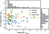 |
Fig. 5. UV magnitude versus spectroscopic redshift for our sample. We show sources from CEERS, JADES, and UNCOVER in blue, orange, and green, respectively. We highlight sources with sufficient S/N(> 15) for robust IGM fitting (see Section 4) with black outlines. |
For each source, in addition to spectroscopic redshift, we measure MUV and [OIII]+Hβ EW. MUV is derived from NIRCam photometry using the filters nearest to the rest-frame 1500 Å, as done by Tang et al. (2023). [OIII]+Hβ EW is derived with prism when the optical continuum has good S/N, or from BEAGLE modelling to NIRCam photometry otherwise (following the approach by Chen et al. 2024). We used the following sources for NIRCam photometric catalogs: the CEERS catalog from Endsley et al. (2023), JADES DR2 (Rieke et al. 2023; Eisenstein et al. 2023a) and UNCOVER DR2 (Weaver et al. 2024), using the lensing map by Furtak et al. (2023) to correct for magnification.
4. Spectral fitting
Here we describe our approach for fitting the prism continuum spectra to recover IGM and local HI properties. We first describe how we forward-model each galaxy’s spectrum after transmission through local HI and the IGM. We then describe our likelihood function which accounts for the covariance in prism spectra and discuss the S/N requirements for recovering robust IGM constraints. We describe the setup for our Bayesian inference and priors in more detail in Appendix D.
We perform the following steps to forward-model prism spectra for each observed source:
-
Create an intrinsic continuum model for < 1500 Å by fitting the observed spectrum at > 1500 Å using the photoionization modelling code BEAGLE (Chevallard & Charlot 2016). By fitting the spectrum including all nebular emission lines, BEAGLE predicts the nebular continuum at < 1500 Å. The BEAGLE fits are performed using a constant star formation history, a Chabrier (2003) IMF (upper mass cut 100 M⊙), Pei (1992) SMC extinction curve (uniform prior on the V-band optical depth from 0 to 6), uniform prior on log U from −4 to −1, and a uniform prior on the ionizing photon escape fraction fesc from 0 − 1. Non-zero escape fractions are required to fit very blue, β < −2.6, UV slopes, as seen in a small fraction of z > 5 spectra (Topping et al. 2024). To test the accuracy of the continuum models we compare the predicted and observed spectra at 1400 − 1500 Å. This is blueward of the range we used to fit the spectrum with BEAGLE but redward of where the IGM and local absorbers can significantly change the continuum. We calculate the residual spectrum over 1400 − 1500 Å (observed – predicted/observed). We find: 1) the distribution of mean (over 1400 − 1500 Å) residuals is peaked at zero, indicating no systematic bias above or below the observed continuum, and 2) the distribution of standard deviations of residuals (equivalent to the fractional error on the continuum models) across our sample has a median at 10% (6–22%, 16–84% range, with the uncertainty decreasing with increasing S/N). A range of dust attenuation laws may also impact the shape of the UV continuum, though we note the majority of our sources are fit with negligible dust attenuation. Deep, high resolution grating spectra of the UV continuum will provide further tests of photoionization models, which will be important future work. Our recovered uncertainties are comparable to the uncertainty on fits to quasar continua at z < 7.5 (∼5 − 10%, Greig et al. 2024a; Hennawi et al. 2025). These recovered errors are however ≈5× higher than the uncertainty of the continuum models output from BEAGLE, so we rescale all output continuum models uncertainties by a factor of five.
-
Add attenuation by local absorbers, τDLA(NHI,eff), with effective column density NH I,eff at the redshift of the source4. As described in Section 2.2 we also consider fits with non-uniform covering fraction, fcov < 1, or with a proximate absorption system along the line of sight. In the majority of sources these do not provide significantly better fits.
-
Add emergent Lyα emission using a single Gaussian emission line with equivalent width EWLyα, FWHM and velocity offset from systemic, Δv. This is the emission before transmission through the IGM, and must be included even in sources without apparent Lyα emission to account for the contribution of weak Lyα which is unresolved by the prism (Jones et al. 2024; Chen et al. 2024; Keating et al. 2024a). Lower redshift studies have shown a large fraction of the variance in Lyα emission can be predicted by galaxy properties linked to the production and escape of Lyα photons (see e.g. Trainor et al. 2019; Hayes et al. 2023) Thus, we use conditional empirical priors for the above Lyα properties as a function of each galaxy’s emission properties (MUV, OIII+Hβ EW), based on z ∼ 5 − 6 observations (Tang et al. 2024a). We describe these priors in more detail in Appendix D.
-
Add resonant scattering attenuation due to gas infalling to the halo. By z ≳ 5 dense residual HI in the ionized IGM resonantly scatters photons emitted blue-ward of Lyα linecenter. Gravitational infall of gas around halos can shift this attenuation red-ward, to approximately the circular velocity of the halo, as Lyα photons appear blue-shifted in the frame of infalling gas (e.g. Santos 2004; Dijkstra et al. 2007). Following Mason et al. (2018b) we cut transmission blueward of the circular velocity of the halo, and add a random scatter of 10%, motivated by hydrodynamical simulations by Park et al. (2021) demonstrating moderate sightline variance.
-
Add attenuation by the neutral IGM at a distance Db from the source: using IGM damping wing optical depths
 drawn from the simulated sightlines described in Section 2.1.1. For each galaxy we draw sightlines from halos in the simulation with UV magnitudes MUV within 0.2 mag of the observed magnitude.
 -
Convolve the model spectrum with the resolution of the prism5.
Thus the final model spectrum given the galaxy parameters θgal is:
 (5)
(5)
where femit is the continuum model (step 1) plus intrinsic Lyα emission (step 2) multiplied by the transmission curve:
 (6)
(6)
where θLyα = (EWLyα, Δv, FWHM) are the Lyα emission parameters (step 2),  are the DLA parameters (step 3) and
  is the IGM optical depth (step 5).
We fit the spectra using Bayesian inference. Because resampling of prism spectra introduces covariance between adjacent pixels (Jakobsen et al. 2022), we use the following likelihood for each source:
![Mathematical equation: $$ \begin{aligned} \ln p(\mathbf f _\mathrm{obs} \,|\, \mathbf \theta ) = -\frac{1}{2}\mathbf r ^\intercal K^{-1} \mathbf r - \frac{1}{2}\ln \left[{2\pi \, \mathrm{det} (K)}\right], \end{aligned} $$](/articles/aa/full_html/2026/01/aa53820-25/aa53820-25-eq49.gif) (7)
(7)
where r = fobs − fmod is the residual vector, K is the N × N covariance matrix6.
Based on estimates of the NIRSpec prism covariance matrix from multiple exposures in the GTO surveys (P. Jakobsen, priv. comm.), we assume the covariance matrix can be approximated as a near-diagonal matrix:
 (8)
(8)
where σi is the observational noise in spectral pixel λi, δij is the Kronecker delta and k is a covariance function between adjacent spectral pixels λi, λj:
 (9)
(9)
i.e. k = 0 if j ≠ i ± 1.
We use Bayesian inference to infer the parameters  , Db and θgal (=θLyα, θDLA) for each galaxy. We note that, since the damping wing fits are most sensitive to Db (see Appendix A), using sightlines labelled with both Db and
  makes the inference of
  for each galaxy explicitly conditional on Db, thereby propagating uncertainties in the inferred Db values into the uncertainties on
  . For z > 10 sources without spectroscopic redshifts from emission lines we also fit for zspec as a free parameter, using a Gaussian prior for the redshift based on an initial fit to the Lyα break. We describe the setup for the inference and priors in Appendix D.
To understand the S/N requirements to obtain robust inferences we perform fits to mock spectra. As described in Section 2.1, to accurately recover information about  requires being able to infer the distribution of distances of each galaxy to the neutral IGM, Db. We find that to robustly recover bubble sizes Db ∼ 5 cMpc (typical of the early stages of reionisation, see Figure 2) with prism spectra requires S/N ≥ 15 per pixel, while log10NH I ≳ 20 can be recovered with S/N ≥ 5 per pixel. Because of the low resolution of the prism we can obtain only upper limits on smaller bubble sizes and column densities. These constraints are vastly improved with higher resolution data, as we discuss in Section 6.3. In Section 6.3 we also discuss prospects for reducing uncertainties in
  with larger samples. We describe the mock tests and validation of our model-fitting in more detail in Appendix E. We plot all individual spectra, their best-fit BEAGLE models, and damping wing fits in Appendix F.
5. Results
We first present empirical results from our sample in Section 5.1, finding the redshift evolution around the Lyα break shows strong evidence for an increasingly neutral IGM. In Section 5.2 we then present our fits to the individual spectra and the inferred evolution of IGM properties.
5.1. Redshift evolution of z > 6 spectra
Studies of Lyα emission in galaxies with JWST NIRSpec have found a decrease in the Lyα EW distribution at z ≳ 7 (Napolitano et al. 2024; Nakane et al. 2024; Tang et al. 2024c; Jones et al. 2025; Kageura et al. 2025), and that strong Lyα emission becomes extremely rare at z ≳ 9 – with only one EW ≳ 15 Å Lyα detection identified (at z ≈ 13, Witstok et al. 2025). If this decline in the Lyα EW distribution is due to damping wing absorption in an increasingly neutral IGM we should expect a corresponding decrease in the UV continuum redward of Lyα. To see how galaxy spectra evolve with redshift around the Lyα break we first consider the evolution of stacked spectra. As we see considerable variance in the spectra, particularly at z ∼ 5.5 − 7, we then construct a ‘mean Lyα transmission’ for each galaxy, ⟨T⟩. We demonstrate the redshift evolution is most likely driven by an increasingly neutral IGM.
We show stacked spectra for our sample in five redshift bins in Figure 6. We redshift the spectra to the rest-frame and normalise each spectrum by the median flux density between 1350 − 1550 Å. We create 100 realisations of each spectrum, sampling from the noise. For the 7 galaxies at z > 10 with redshift only from the break, in each realisation, we also sample a redshift based on the uncertainty from fitting the Lyα break. For sources with optical line detections the typical spectroscopic redshift uncertainty (σz ∼ 0.002) is sub-pixel for z ∼ 5 − 14 Lyα breaks (where one prism wavelength pixel corresponds to Δz ∼ 0.05 − 0.15) thus redshift uncertainties will not add significant uncertainty to the stacks. We resample all spectra onto a common wavelength grid with pixel size 10 Å and then stack in wavelength and redshift bins. Our stacks show the median and 16–84% range of the normalised spectra in each wavelength pixel.
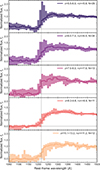 |
Fig. 6. Median stacked spectra in our sample of 99 sources in redshift bins. Shaded regions show the 16–84% range of the spectra in each redshift bin. We see a clear decrease in flux and the variance of the spectra around the Lyα break with increasing redshift. |
Figure 6 shows a clear decrease in both the median and variance (the shaded 68% range) of flux around Lyα with increasing redshift. These stacks show: 1) at z < 6 the 16th percentile range of the stack shows positive flux blueward of Lyα (∼1050 − 1150 Å, though with lower flux closest to line center as predicted due to gravitational infall Laursen et al. 2011), implying the majority of galaxies transmit some flux blueward of Lyα, but at higher redshifts the median flux blueward of Lyα is consistent with zero. We can also see this excess in individual spectra in Figure F.1. This implies the IGM is not completely optically thick at the Lyα resonance at z < 6 ( ), as expected from quasar Lyα forest observations (e.g. Eilers et al. 2019; Bosman et al. 2022). Recent JWST analyses by Meyer et al. (2025) and Umeda et al. (2025a) have quantified this excess flux seen in prism spectra z < 6 in more detail, and find it is consistent with measurements in quasars; 2) a rapid decrease in strong Lyα emission at z ≳ 6; 3) fully ‘damped’ spectra at z > 8, consistent with results in a smaller sample by Umeda et al. (2024).
To assess the relative contribution of local absorption and IGM absorption to the decline in transmission, in Figure 7 we plot the fraction of our sample with spectra consistent with a neutral IGM, and the fraction of strong DLA candidates (i.e. absorption stronger than the neutral IGM). We select sources as consistent with neutral IGM if the observed spectrum around the break is at least 1σ lower, in at least 3 consecutive wavelength pixels, than the predicted continuum in an ionized IGM, convolved with the prism resolution, in a fully ionized IGM at the redshift of the source (Section 4, step 1). We select sources as strong DLA candidates if the observed spectrum around the break is > 1σ lower, in at least 3 consecutive wavelength pixels, than the predicted continuum in a fully neutral IGM at the redshift of the source (Section 4, step 1 + 5). This corresponds to DLAs with NH I ≳ 1021 cm−2 at z ∼ 6 and NH I ≳ 1021.5 cm−2 at z ∼ 14, irrespective of whether the source is an ionized region or not, as the DLA absorption becomes stronger than the IGM alone at these column densities (see Figure 4 and Figure B.1). Uncertainties on the fractions are calculated using Poisson statistics.
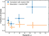 |
Fig. 7. Fraction of sample showing spectra consistent with fully neutral IGM attenuation (blue points) and with absorption stronger than the neutral IGM, i.e. strong DLAs (orange points). While the fraction of strong DLA candidates drops slightly with redshift, the majority of z > 9 spectra are consistent with a neutral IGM. |
Figure 7 shows the fraction of strong DLA candidates is 0.25 ± 0.09 at z ∼ 5.5 − 6 and 0.19 ± 0.11 at z > 9, indicating minimal evolution in local absorption systems with increasing redshift which we discuss further in Section 6.2. By contrast, the fraction of spectra consistent with neutral IGM increases significantly from 0.36 ± 0.11 at z ∼ 5.5 − 6 to 0.81 ± 0.23 at z > 9. Of the 12 z > 9 spectra in our sample, only three (jades-1181-3991 (GNz11), ceers-2750-64, and jades-3215-20128771) have spectra showing emission in excess of the prediction for a neutral IGM. We further explore some simple physical models for the evolution of the stacked spectra in Appendix C, finding the evolution is most consistent with the majority of the redshift evolution being driven by the neutral IGM evolution.
To explore the variance we observe in the spectra (Figure 6) in more detail, in Figure 8 we show the mean transmission ⟨T⟩ over the Lyα-break (1215 − 1230 Å rest-frame, corresponding to a contribution from two wavelength pixels in the prism for all sources in our sample) for each galaxy as a function of redshift. The transmission is calculated as the ratio between the observed spectrum and the continuum model (see step 1, Section 4, excluding Lyα emission, DLAs, or IGM absorption, corresponding to the thick blue lines in Figures F.1–F.4) for each source. Using this definition ⟨T⟩> 1 corresponds to Lyα emission, and ⟨T⟩< 1 is absorption. ⟨T⟩< 0 corresponds to negative flux in the observed spectra due to noise fluctuations. We show the median and 68% range as error bars obtained from 1000 realisations of both the observed spectrum, resampling from the error spectrum, and the posterior for model continuum spectrum (see step 1, Section 4 for more details on the uncertainty in the model continuum), convolved with the resolution of the prism. To calculate the transmission the spectra are rebinned on a common wavelength grid with wavelength pixel 5 Å. Because of the sensitivity of this to the precise spectroscopic redshift, we only include sources with redshifts measured from emission lines in Figure 8. We show the mean transmission for individual galaxies in grey as well as the median and 68% range in 5 redshift bins. We find both the median ⟨T⟩ and its 68% range, as shown by the coloured points, decrease with redshift:  at z < 6, falling to
  at z > 10. In particular, we see a strong decline in ⟨T⟩> 1 for individual sources, which corresponds to a decline in strong Lyα emission.
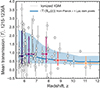 |
Fig. 8. Mean transmission, ⟨T⟩, over 1215 − 1230 Å rest-frame for each galaxy in our sample (grey circles), as a function of spectroscopic redshift, including only sources with redshifts from emission lines. ⟨T⟩ corresponds to the flux around the Lyα break relative to the predicted galaxy continuum in an ionized IGM, with no contribution from Lyα emission or absorption by HI. Thus ⟨T⟩> 1 corresponds to Lyα emission, and ⟨T⟩< 1 to absorption. We show the median and 68% range of ⟨T⟩ in four redshift bins (coloured circles). The blue line and shaded regions shows the predicted median and 68% range of ⟨T⟩ assuming the z ≲ 6 template spectra described in Section 5.1 and the reionisation history inferred by Mason et al. (2019). The observed median and range are in close agreement with the IGM prediction. |
At z ∼ 7 − 8 the median stacked spectrum at ≈1216 Å is higher than at all other redshifts (solid line in Figure 6) and we see the transmission is comparable to z ∼ 6 − 7 (Figure 8). We attribute this to cosmic variance in the IGM. This redshift bin is dominated by the large number of sources (6/11 sources) in the CEERS/EGS field, which hosts the largest number of Lyα-emitters known at z > 7 and is likely a large ionized region (e.g. Tilvi et al. 2020; Larson et al. 2022; Jung et al. 2024; Chen et al. 2024; Tang et al. 2023, 2024c; Napolitano et al. 2024). We discuss the impacts of cosmic variance in Sections 6.1 and 6.3.
We compare our observed ⟨T⟩ with a prediction for the IGM transmission assuming the median reionisation history  inferred by Mason et al. (2019), based on the Planck Collaboration VI (2020) CMB optical depth and the Lyα forest dark pixel estimates of
  at z < 6 by McGreer et al. (2015) (blue line and shaded region showing median and 68% range). To model ⟨T⟩ we create template spectra at z < 6, using the fits to our z < 6 sample to create high resolution model spectra which include local absorption (see more details in Appendix C), and apply Lyα damping wings drawn from our IGM simulations (described in Section 2.1.1) given the IGM neutral fraction predicted as a function of redshift, assuming no evolution in local NH I, as motivated by Figure 7 and our analysis in Appendix C. For each template z < 6 galaxy we draw damping wings to galaxies within 0.2 mag of its UV magnitude, to account for brighter sources being more likely to be in bigger bubbles. Our prediction on ⟨T(z)⟩ is mostly determined by the overall IGM state given by
  , as the dependence on MUV is sub-dominant (Mason et al. 2018b), especially given the median magnitude of the sample does not change significantly with redshift (MUV ≈ −19.3 at z < 6 to MUV ≈ −19.7 at z > 8). We convolve these to the prism resolution and calculate ⟨T⟩ as described for the observed spectra.
We plot the median and 68% range of the predicted ⟨T(z)⟩ as the blue line and shaded region on Figure 8, where the range is a direct consequence of the size distribution of ionized regions with increasing redshift (Figure 1). The median and 68% range of the observed ⟨T⟩ closely tracks this prediction for an increasingly neutral IGM, excluding the z ∼ 7 − 8 bin. In particular, the decline in the variance of ⟨T⟩ with redshift is consistent with the expectations for an increasingly neutral IGM: in the late and mid-stages of reionisation  (z ≲ 7), most observable galaxies reside in ionized regions (Lu et al. 2024), meaning we can still expect to detect strong Lyα emission. In the earliest stages of reionisation at z ≳ 9, ionized regions become too rare and small to transmit significant flux, thus both the median and variance of ⟨T⟩ drops significantly (e.g. Mason et al. 2018a).
These results are consistent with the previous JWST analyses which have found a decrease in strong Lyα emission with increasing redshift (Nakane et al. 2024; Tang et al. 2024c; Jones et al. 2025; Kageura et al. 2025), and increase in the strength of the Lyα break with redshift (Umeda et al. 2024). Our results are qualitatively consistent with those of Heintz et al. (2024a) who explored the evolution of the Lyα break in a larger sample, though with a lower S/N threshold, finding a decrease in Lyα emission with increasing redshift and no strong evolution in the abundance of strong DLA candidates. Our results are also consistent with an analysis of photometry by Asada et al. (2025), who find an increase in an effective NH I parameter (combining IGM and DLA damping) of ∼1 dex from z ∼ 6 − 10, which can be produced by the transition to mostly neutral IGM (Figure 4).
Our results demonstrate a clear reduction in the median and variance of flux around the Lyα break with increasing redshift, dominated by a decline in strong Lyα emission at z > 8, with no significant evolution in the fraction of strong DLAs with redshift, implying the IGM drives the redshift evolution evolution. The majority of the spectra are consistent with a fully neutral IGM at z ≳ 9.
5.2. IGM constraints from spectral fitting
We now select a sub-sample of our spectra with sufficient S/N to perform robust damping wing fits to obtain more quantitative constraints. Based on fits to mock spectra (see Section 4 and Appendix E) we select sources with S/N ≥ 5(15) per pixel where we can obtain robust NH I(Db) estimates. This results in a subsample of 83(14) sources with S/N ≥ 5(15), with 6 at z > 9. We fit each galaxy’s spectrum as described in Section 4 and show the resulting fits to individual spectra in Appendix F.
As an example, we show the fit for jades-3215-265801 at z = 9.44 (Bunker et al. 2024; Curti et al. 2025) in Figure 9. This is one of the highest S/N (≈30 per pixel) spectra in our sample and shows a clear attenuation around the Lyα break relative to the expectation from the > 1500 Å spectral fit (blue line and shaded region showing continuum model uncertainty). Our fit recovers a distance from neutral IGM,  resulting in a strong lower limit on
  (1σ). Fixing fcov = 1 we infer a local absorber HI column density
  , and obtain
  allowing fcov < 1. These results are consistent with the recent analysis by Curti et al. (2025) who did not consider fcov < 1. The corner plot highlights there is a degeneracy between Db and NH I (and thus also
  ), but the spectrum does constrain these parameters. We show the fit using without including neutral IGM as a green line, showing the local absorber produces too much flux redward of Lyα, demonstrating that a high
  (low Db) is required to better explain this spectrum. A higher column density absorber would reduce the flux at line center and be inconsistent with the observed spectrum. The shape of the 2D posterior for
  reflects our prior
  (see Figure 2), whereby a low inferred Db implies high
  , and vice versa. In this way, damping wing constraints on Db can be directly linked to
  , propagating the uncertainty on Db self-consistently. As discussed in Section 2.1 this mapping – as for all
  estimates using damping wing transmission – depends on the reionisation morphology. However, as demonstrated by Greig et al. (2017, 2019), the inferred
  is not expected to be significantly biased by the choice of reionisation morphology. This is because, to first order,
  is the most important factor in determining the reionisation morphology, irrespective of the ionizing source model (McQuinn et al. 2007). We see the IGM and Lyα parameters are not sensitive to our fcov prior: the IGM damping impacts redder wavelengths than a DLA and the source shows no hint of Lyα emission at the resolution of the prism so we recover our priors.
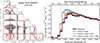 |
Fig. 9. Fitting the spectrum of the z = 9.44 galaxy jades-3215-265801. Left: 2D posteriors for |

To estimate  as a function of redshift from our sample we combine the marginalised posteriors on
  for each galaxy (Appendix D). We create two redshift bins at zbin = 5.5 − 8, > 8 (containing 8 and 6 galaxies respectively) to obtain
  . We find
  at z ∼ 5.5 − 8.0, 8.0 − 10.6 (⟨z⟩ = 6.5, 9.3). We recover
  excluding GNz11. The uncertainties include a conservative addition of
  to account for sightline variance given we have sampled only 3 fields (see Section 6.3). Figure 10 shows our inferred timeline of reionisation, including an additional uncertainty due to cosmic variance in the IGM (see Section 6.3), along with other estimates from the literature which infer
  using inhomogeneous reionisation simulations, based on: the Lyα equivalent width distribution in Lyman-break galaxies (EW, Mason et al. 2018b, 2019; Whitler et al. 2020; Bolan et al. 2022; Tang et al. 2024c; Kageura et al. 2025), the clustering of Lyα emitters (Sobacchi & Mesinger 2015), and quasar damping wings (Davies et al. 2018; Greig et al. 2019; Wang et al. 2020); and the Lyα forest dark pixel fraction (Jin et al. 2023). Our results show a clear increase in the inferred neutral fraction with increasing redshift, albeit with large uncertainties.
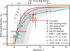 |
Fig. 10. Timeline of reionisation: Volume-averaged mean hydrogen neutral fraction as a function of redshift. Our new constraints are plotted as red pentagons and error bars, light red error bars include the additional uncertainty due to IGM cosmic variance (Figure 14). The filled red pentagon is the lower limit we obtain excluding GNz11 from our sample. We also plot, as grey points, constraints on |

For comparison, we also show the space of  allowed by the Planck Collaboration VI (2020) optical depth and McGreer et al. (2015) Lyα forest dark pixel fraction constraints as inferred by Mason et al. (2019), along with three simple reionisation history models (following e.g. Madau et al. 1999) which all end around z ∼ 6: (1) integrating the Mason et al. (2023) UV LF model down to MUV < −13, assuming constant ionizing photon escape fraction of 6%, (2) only including galaxies down to MUV < −20, assuming constant ionizing photon escape fraction of 20%, which produces the most rapid reionisation; (3) the same as model (1) but fixing the UV luminosity density of the model at z ≥ 9 to approximate JWST UV LF results (e.g. Donnan et al. 2024; Whitler et al. 2025). We discuss our results in the context of our understanding of reionisation in Section 6.1.
6. Discussion
JWST has opened a unique new window on the earliest stages of reionisation by providing deep rest-frame UV to optical spectroscopy of z ∼ 6 − 14 galaxies. In Section 6.1 we discuss our results in the context of our understanding of reionisation. In Section 6.2 we discuss the nature of local neutral hydrogen absorption systems and in Section 6.3 we discuss future prospects for improving IGM constraints from galaxy damping wings.
6.1. The reionisation process
Our empirical constraints from the stacked spectra and mean transmission (Section 5.1) imply the IGM is approaching almost fully neutral at z ≳ 9. Our inferred constraints on  (Section 5.2) also imply a mostly neutral IGM at z ≳ 8. These results are independent confirmation of previous ground-based efforts to constrain the reionisation history at z > 7 via the damping wing attenuation in quasars (Davies et al. 2018; Wang et al. 2020; Greig et al. 2024b) and decline of Lyα emission in Lyman-break galaxies (Stark et al. 2010; Schenker et al. 2014; Mason et al. 2019; Bolan et al. 2022). These results are also in agreement with recent independent analyses of JWST data based on the decline in the Lyα EW distribution (Tang et al. 2024c; Kageura et al. 2025) and damping wings (Umeda et al. 2024; Park et al. 2025) which also point to a highly neutral IGM at z ≳ 8. Our approach builds on early JWST damping wing analyses by including additional sources of uncertainties and mapping spectra to
  based on inhomogeneous IGM simulations.
Mostly strikingly, in Section 5.1 we showed the spectra demonstrate a decrease in both the mean and variance of Lyα transmission with increasing redshift. We interpret this as due to the decrease in size and variance of ionized regions with increasing redshift, as expected in the earliest stages of reionisation (e.g. Mesinger & Furlanetto 2007; Iliev et al. 2007). Tang et al. (2024c) also find a decrease in the median Lyα EW and variance of the EW distribution with redshift, which likely reflects the same signal. This can be seen as analogous to the decrease in the mean and variance of effective optical depths in the Lyα forest at z ≲ 6 (Eilers et al. 2019; Bosman et al. 2022) which mark the end of inhomogeneous reionisation as the mean and variance in the sizes of neutral regions decrease (e.g. Keating et al. 2020). Our results provide evidence we are now observing this process in reverse – probing the earliest stages of reionisation.
In Figure 10 we show our  estimates along with previous constraints and simple theoretical models for the reionisation timeline. At z ∼ 5.5 − 8 our constraints are fully consistent with pre-JWST constraints from a number of independent probes (quasar damping wings, Lyα forest dark pixel fraction, Lyα EW distribution, Lyα-emitter clustering). At z > 8 our
  constraint is slightly lower than, though consistent within error bars, the constraint by Tang et al. (2024c) obtained from the Lyα EW distribution in 48 z > 8 galaxies the JWST public archive, the largest sample to date used to constrain
  at z > 8. If we exclude GNz11 our constraint on
  at z > 8 is a lower limit,
  (68% credible interval), driven mostly by the constraint from jades-3215-265801. We attribute the difference between our result and that of Tang et al. (2024c) to several factors: our sample is significantly smaller due to our requirement of S/N > 15 prism spectra at z > 8 (just 6 sources), meaning we are more subject sample selection; most of our sources return low significance
  constraints due to the moderate S/N; and finally, by fitting both IGM and local HI properties jointly we allow some of the decrease in transmission to be explained by local absorption (see e.g. Figure 9).
Upcoming Cycle 3 NIRSpec surveys (Dickinson et al. 2024; Oesch et al. 2024) will significantly increase the sample of spectroscopically confirmed z ≳ 10 galaxies to ≳100. High S/N spectra in these samples will hugely improve our ability to learn about the IGM at these redshifts, both via damping wing approaches as we have described, and the Lyα EW distribution. In the future, with larger samples, it could be most informative to infer distributions of Db, rather than  , as a function of redshift to different simulations, as this should track the size evolution of ionized regions in a model-independent way and shed light on the morphology of reionisation.
The z ≳ 10 IGM contains key information about early star formation. In particular, models which end around the same time at z ∼ 6 can be driven by very different sources, but diverge at z > 9, highlighting the importance of constraints on the IGM at these high redshifts. In Figure 10 we show a reionisation history corresponding to if the excess in the UV luminosity density observed with JWST holds down to low luminosities, as indicated by deep observations (Pérez-González et al. 2023; Robertson et al. 2024; Whitler et al. 2025). In this case, reionisation could start early, and the IGM could be already ∼20% ionized at z ∼ 10 (see also Gelli et al. 2024). This is interesting to note in relation to recent CMB analyses indicating the electron scattering optical depth may be higher than measured by Planck Collaboration VI (2020) (Pagano et al. 2020; de Belsunce et al. 2021; Giarè et al. 2024). As discussed by Asthana et al. (2024), an early start to reionisation is not inconsistent with the requirement from the Lyman-α forest that reionisation is complete by z ∼ 5.3 − 6. Current z ≳ 8 constraints, the tightest coming from the evolution of the Lyα EW distribution (Nakane et al. 2024; Tang et al. 2024c; Jones et al. 2025; Kageura et al. 2025), all imply a mostly neutral IGM at z > 8 (e.g.  at z ∼ 8 − 10 Tang et al. 2024c), but do not yet reach the precision to rule out that the IGM may already be ∼10% ionized at z ∼ 10. Future observations with large samples of deeper spectra will improve our estimates of
  (see Section 6.3), providing important constraints on the onset of star formation.
6.2. Nature and evolution of local absorbers
In addition to neutral IGM, our sample demonstrates absorption due to HI gas within, or in close proximity to, the galaxies, as damped Lyα absorbers (DLAs). As described in Section 2.2, the existence of strong local absorption is not unexpected: HI dominates the volume of most galaxies, indeed the Milky Way disk is NH I ∼ 1022 cm−2 (Kalberla & Kerp 2009), and the massive stars which dominate our spectra are likely to reside in the densest regions of the ISM and experience high HI columns. Evidence for neutral gas in the ISM and CGM of galaxies is observed both in absorption and emission over a wide range of redshifts at z ∼ 0 − 6 (e.g. Shapley et al. 2003; Steidel et al. 2010; Wisotzki et al. 2016; Tanvir et al. 2019; Pahl et al. 2020; Krogager et al. 2024). These observations of both absorption features and Lyα emission (whose lineshape is primarily set by NH I e.g. Verhamme et al. 2015) imply high column densities of neutral gas in the ISM and/or CGM (with median NH I ∼ 1020.3−21.0 cm−2 in z ∼ 3 LBGs, Reddy et al. 2016), though likely with non-uniform covering fractions (and low dust sightlines) enabling high EW Lyα escape close to systemic velocity in some galaxies (e.g. Shapley et al. 2003; Heckman et al. 2001; Du et al. 2018; Hu et al. 2023; Tang et al. 2024b).
JWST has extended the detection of DLAs in galaxy spectra to z > 5 (e.g. Heintz et al. 2024b, 2025; Chen et al. 2024; Hainline et al. 2024; D’Eugenio et al. 2024), providing evidence for some systems with column densities log10 NH I ≳ 22. As described in Section 2.2, only systems with column densities NH I ≳ 1022 cm−2 become challenging to distinguish from IGM absorption. Such high column densities may be expected in the regions around young stars, before stellar feedback begins to disperse dense birth clouds. High resolution radiative hydrodynamic simulations predict NH I∼1021−23 cm−2 in these regions, and that feedback should open low density channels (i.e. a non-uniform covering fraction) and finally disperse the cloud within ≲10 − 40 Myr (Kimm et al. 2019; Ma et al. 2020; Kakiichi & Gronke 2021), though the feedback mechanisms are still debated. Additionally, considerable opacity may come from the dense filaments and/or clumps in the CGM and local environment of massive halos (e.g. Rudie et al. 2012; Turner et al. 2017).
In the context of reionisation, it is important to understand to what extent the opacity due to local HI evolves with redshift and can impact IGM constraints. We first explore the nature and evolution of Lyα opacity due to local HI in our sample. We then discuss the impact of the decreased UV background during reionisation on the Lyα opacity within ionized regions.
In Figure 11 we show the inferred HI column densities for our sample, obtained from fitting 83 S/N > 5 spectra as described in Section 4, after marginalising over the IGM attenuation. We also show the median and 68% range, obtained from sampling the posteriors of our fits, of NH I in 4 redshift bins. We find no significant redshift evolution over z ∼ 5.5 − 8, similar to constraints by Heintz et al. (2024b) and Umeda et al. (2024), with a slight decrease at z > 8. This is consistent with our empirical constraint in Figure 7. We find a median NH I = 1020.8 cm−2, comparable to z ∼ 3 LBGs (Reddy et al. 2016), with a broad range consistent with observations from GRB sightlines (Tanvir et al. 2019), which probe the ISM around massive stars. We find NH I is somewhat sensitive to the Lyα emission prior (Appendix E), finding median NH I = 1020.4 cm−2 if we use essentially a conditional prior on Lyα emission given NH I, but that the redshift trend is unchanged.
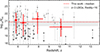 |
Fig. 11. Inferred local HI column density as a function of redshift. Grey points show the median and 68% range inferred from fits to individual spectra. Red markers show the median and 68% range in four redshift bins. The grey shaded region shows the range of NH I estimated in median stacked spectra of ∼1000 z ∼ 3 LBGs by Reddy et al. (2016). |
While the median NH I we infer is similar to z ∼ 3 results, we do find a broad distribution. Consistent with our empirical findings that ≈20% of sources with breaks stronger than the neutral IGM alone, Figure 7), we find 18% of sources with median NH I ≳ 1022 cm−2, though the uncertainties are large7. Only 6 sources (8% of the sample) have 68% confidence intervals which do not extend below NH I < 1022 cm−2. These sources are: jades-1210-13176, which shows both Lyα emission and the most extreme damped profile in our sample (this has been previously discussed byCameron et al. 2023; Terp et al. 2024; Tacchella et al. 2025, as potentially a nebular continuum dominated source, high NH I proximate DLA, or AGN respectively. We find it can be fit well using a non-uniform covering fraction (Figure F.1)); two sources in an extreme overdensity at z = 7.88 in Abell 2744 (Morishita et al. 2023), previously identified by Chen et al. (2024), including one with Lyα emission; two sources which also show Lyα emission (jades-1210-9880 and uncover-4-36755) and ‘damped’ profiles. However, potential absorption is present only in 3 pixels redward of Lyα and the fits appear to overestimate the damping (Figure F.2), thus we do not consider these 2 sources robust DLA candidates; and finally, ceers-P7Pr-1023 (z = 7.78) which shows a strong damped profile with log10 NH I = 22.5 ± 0.2 and no Lyα emission. Tang et al. (2023) noted this source is red (β = −0.9) suggesting significant dust, which is usually correlated with high NH I at lower redshift (Reddy et al. 2016). The presence of Lyα emission plus absorption in 4/6 of these candidates hints at non-uniform covering fractions caused by young stars starting to disperse their birth clouds, or alternative explanations such as strong nebular emission (Katz et al. 2025).
We now consider the possible origins of moderate column density local DLAs (NH I ≳ 1021 cm−2) in our sample. We examine the z < 6 sub-sample, where the IGM damping wing impact is expected to be minimal. We use a simple selection of DLA candidates following the approach described in Section 5.1. We select sources where the observed spectrum around the break is at least 1σ lower than the BEAGLE predicted intrinsic continuum (Section 4), including uncertainties in both the observed spectrum and predicted continuum, in a fully neutral IGM at the redshift of the source in at least 3 consecutive wavelength pixels, corresponding to DLAs with NH I ≳ 1021 cm−2 (Figure 4). This selection is consistent with the results of Figure 11 but allows us to individually inspect every source, as some spectra show artifacts which could bias the damping wing fits.
We first examine whether there is a correlation between DLA candidates and dust attenuation, which could indicate absorption by dense gas in the source galaxy. Reddy et al. (2016) found that high neutral hydrogen column densities and covering fractions correlate with reddening by dust in z ∼ 3 Lyman-break galaxies, which would be expected if high dust fractions trace high gas fractions. Apart from ceers-P7Pr-1023, we do not find our DLA candidates have significantly higher dust attenuation, based on our BEAGLE fits, compared to our full sample. However, the majority of our sample have very low dust attenuation. If the absorbing gas is located in the ISM this suggests low metallicity or low dust-to-gas ratios (consistent with the declining UV beta slopes at z > 7 observed with JWST, Topping et al. 2024; Cullen et al. 2024; Morales et al. 2024), see also Tacchella et al. (2025). This is consistent with recent observations by Tang et al. (2024a) of Lyα line profiles at z ∼ 5 − 6, finding strong Lyα-emitters (EW > 40 Å) have high Lyα velocity offsets from systemic (median Δv ≈ 230 km/s), implying scattering in NH I ∼ 1019−20 cm−2 gas with a high covering fraction and low dust opacity (Laursen et al. 2009; Verhamme et al. 2015).
We also consider whether Lyα absorption is enhanced in close associations (≲500 pkpc) of galaxies, which should trace the most massive halos (Mh ∼ 1011 − 12 M⊙, Rvir ∼ 25 − 50 pkpc) and protoclusters, where hydrodynamic simulations predict both an increased prevalence of filaments and dense neutral gas in the CGM, and higher gas mass in the ISM which could provide high opacities from star-forming regions (e.g. Stern et al. 2021; Tortora et al. 2024; Gelli et al. 2025) and z ∼ 2 − 3 observations suggested enhanced absorption (e.g. Turner et al. 2017). Chen et al. (2024) recently discovered three sources in an association of > 10 galaxies within r ≲ 60 pkpc at z ≈ 7.9 in the Abell 2744 field (consistent with a protocluster forming in a Mh ≳ 4 × 10¹¹ M⊙ halo, Morishita et al. 2023) show strong Lyα absorption. We test this hypothesis more systematically in GOODS-S which has the highest density of spectroscopy of any field observed by JWST to date. We focus on zspec = 5 − 6 as the spectroscopic samples are largest here and the IGM damping wing should be minimal. In Figure 12 we show the positions of our sample, highlighting DLA candidates (defined as above) with red circles, along with spectroscopically confirmed galaxies from JADES and FRESCO (Oesch et al. 2023; Tang et al. 2024a; Meyer et al. 2024; Covelo-Paz et al. 2025).
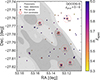 |
Fig. 12. Positions of the z = 5.5 − 6 subset of our sample in GOODS-S. We highlight our sample with stars and additional spectroscopically confirmed sources at z = 5 − 6 from JADES and FRESCO as coloured points. Photometric candidates from JADES with zphot = 5 − 6 are show as grey points, with grey shading marking their density distribution. DLA candidates (as described in Section 6.2) are marked with red circles with projected radii of 30 and 100 pkpc (≲16″). The DLA candidates are more likely to have nearby neighbours (both in projection and physical distance) compared to sources which do not show strong damping wing signatures. |
We see the majority of DLA candidates have close neighbours both in projection and 3D. We find all 6 DLA candidates in GOODS-S have close spectroscopically confirmed foreground neighbours (≲12″, corresponding to impact parameter, b ≲ 75 pkpc). In 5/6 cases these neighbours are offset in redshift by Δz ≲ 0.01. This corresponds to 3D separation < 500 pkpc, thus likely to be physically associated (Chiang et al. 2017) and/or could act as proximate absorbers. Furthermore, several of these 5/6 DLA candidates have multiple close neighbours in 3D: jades-1210-13577 (z = 5.575) has one neighbour within a 3D radius of 200 pkpc (z = 5.573) and sits directly behind (impact parameters < 10 pkpc) a close association of three sources at z = 5.567; jades-3215-99671 has three neighbours within 500 pkpc, including one with impact parameter ≈8 pkpc; jades-1210-13176 also has three neighbours within 500 pkpc, including one with impact parameter ≲1 pkpc; The only DLA candidate without close neighbours in 3D, jades-1210-15099 (z = 5.777) has a foreground source with an impact parameter of 75 pkpc, but the redshift of the foreground source (z ≈ 5.1) is too low to to be physically associated or to act as a proximate DLA (we find a best-fit proximate DLA would lie at z ≈ 5.72). There are no obvious spectral features which distinguish this source from the other DLA candidates. Of the 12 sources in our sample at this redshift range with no strong DLA signature, only 6/12 have neighbours within < 500 pkpc.
This adds increasing evidence that strong DLA systems are associated with more massive halos. However, the prism resolution (spectroscopic redshift uncertainty typically σz ∼ 0.002) means the uncertainty in line of sight distance is ≳100 pkpc: better characterising these environments will require R ≳ 1000 spectroscopy. We should then expect the prevalence of strong DLAs to decrease at higher redshifts as halos assemble hierarchically. We see tentative evidence for this in Figures 7 and 11, but larger samples will be required to confirm this.
Finally, we discuss the impact of increased opacity due to lower column density absorbers in the ionized IGM. Observations of the Lyα forest have revealed the UV background photoionization rate drops by a factor ∼10 at z ∼ 5 − 6 (Becker & Bolton 2013; Gaikwad et al. 2023; Davies et al. 2024), as expected at the end stages of reionisation before ionized regions fully merge. Hydrodynamical simulations predict a corresponding increase of Lyman-limit and sub-DLA absorption systems in ionized regions at z ∼ 5 − 6 (NH I ∼ 1017−19 cm−2, Bolton & Haehnelt 2013; Nasir et al. 2021) as the lower UV background reduces the density threshold for self-shielding. However, a substantial increase in DLAs (NH I > 1020.3 cm−2) is not predicted as those systems are already dense enough to self-shield. As we showed in Figure 4, NH I < 1020.3 cm−2 absorbers are subdominant to the neutral IGM damping wing at ≳1220 Å. An increase in sub-DLAs and LLS can suppress Lyα emission (Bolton & Haehnelt 2013; Weinberger et al. 2019); however Mesinger et al. (2015) demonstrated that evolution in the neutral IGM dominates the opacity, assuming Lyα is offset by Δv ≳ 200 km/s from systemic, where the damping wing from sub-DLAs is minimal. At z ≳ 5 such high offsets appear common, even in strong Lyα emitters: with Tang et al. (2024a) finding a median Δv ≈ 230 km/s in strong Lyα emitters (EW > 40 Å). Thus we do not expect our results to be significantly impacted by an increase in opacity in the ionized IGM.
We conclude that current data suggest no strong redshift evolution of local HI column densities at z ∼ 3 − 13. Future deep, high resolution NIRSpec spectra could provide more insights into the location and nature of absorbing gas, by measuring damped Lyα troughs to determine the redshift of absorbing gas, detecting low ionization interstellar absorption lines, which trace high HI columns and covering fractions in the host galaxy (e.g. Shapley et al. 2003), and could also be used to determine the redshift of proximate absorbers (e.g. Christensen et al. 2023; Davies et al. 2025). High resolution NIRSpec spectra would also provide crucial tests for continuum models.
6.3. Future prospects
With the exquisite spectroscopic capabilities of JWST, the prospects for using galaxies to probe the earliest stages of reionisation at z > 9 are promising. We first discuss prospects for improving our understanding of the impact of the IGM, Lyα emission and local absorbers on prism spectra with higher S/N and higher spectral resolution data, and then discuss the prospects for both overcoming and utilising cosmic variance in the IGM.
Firstly, the most obvious improvements to our approach for fitting IGM damping wings will come from higher S/N and higher resolution spectra. While we see clear evolution in the spectral stacks and evolution of the mean transmission around the Lyα break, fitting the damping wings is still challenging for most sources in the public archive given the low S/N of the spectra. In Appendix E we demonstrate we require S/N per pixel ≳15 to gain unbiased constraints on Db from prism spectra, which can thus be mapped to constraints on  providing we sample a sufficient number of galaxies, which we discuss below. However, even with very high S/N, the prism provides a rather blunt view of the IGM: we find a median uncertainty of ≈0.5 dex on Db in our tests with S/N = 100 per pixel. Our knowledge is limited by the R ∼ 40 resolution of the prism at ∼1 μm, where the impact of the damping wing is compressed into ∼5 spectral pixels (see Figure 3). Therefore, while prism spectra provide a powerful initial view of the early stages of reionisation (e.g. Curtis-Lake et al. 2023; Umeda et al. 2024), a full understanding requires higher resolution spectroscopy and precise constraints on the evolution of Lyα emission with redshift (e.g. Nakane et al. 2024; Tang et al. 2024c).
At higher resolution, constraints on Db using our damping wing fitting approach become much more precise. We demonstrate this in Figure 13 where we show the number of galaxies required to constrain  using either the prism or G140M gratings (see also Appendix E). As described in Section 2.1, constraints on
  effectively come from measuring the distribution of Db at a given redshift and comparing it to predictions from simulations (e.g. Figure 2). To investigate the number of galaxies required to robustly infer
  , we sample Db from the distributions in our simulations at a given
  (Section 2.1.1, shown as dotted lines in Figure 13), and calculate the median Db we would recover from N mock galaxies using our approach. For this forecast, we assume S/N ≈ 20 per pixel for the prism and S/N ≈ 5 for the grating. We chose these values based on our tests to mock spectra (Appendix E), where we recover an average uncertainty on Db of ≈0.7 and ≈0.3 dex for the prism and G140M observations respectively. We sample Db from the simulated
  distributions, additionally sampling from the Gaussian uncertainties on Db given above, for 200 realisations of N galaxies. In this way, our forecasts account for both the measurement uncertainty on Db and the broad
  distribution predicted by the simulations. We find G140M observations can constrain
  with ≳6 galaxies, compared to ≳20 galaxies with the prism. Current grating spectra do not reach this S/N in the rest-frame UV but a S/N ≈ 5 spectrum for mAB = 26 source would require ∼30 hr integration in G140M, feasible for the brightest z > 8 sources. The increase in precision expected with grating spectra is due to the increased resolution around the Lyα break, enabling a better estimate of the IGM damping wing (see Figure E.1).
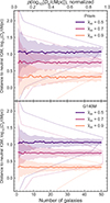 |
Fig. 13. Forecasted number of galaxies required to constrain |


Ultimately, higher resolution spectroscopy will provide the best constraints on early IGM properties as weak Lyα emission can be resolved, which is most sensitive to the IGM opacity in the early stages of reionisation (see Figure 3). Furthermore, grating spectroscopy will provide important validation of our approach for marginalising over Lyα emission in prism spectra and better distinguish the impact of local absorbers. In the prism the Lyα line is spread over most of the pixels including the damping wing feature (see Figure 3 and Keating et al. 2024a; Park et al. 2025). Jones et al. (2024) and Chen et al. (2024) showed this limits the minimum detectable Lyα EW of ≳50 Å for galaxies with our median MUV ∼ −19. Thus, accurate estimates of  and NH I using our approach in prism spectra rely on accurate models, or direct measurements, of the emergent Lyα emission (see Section 4). While significant progress has been made since the launch of JWST in linking Lyα emission to other observables (e.g. Prieto-Lyon et al. 2023; Chen et al. 2024; Tang et al. 2024a), which we have utilised here, deep NIRSpec grating spectra can easily resolve weak Lyα emission (see Figure 3, e.g. Saxena et al. 2024). In high S/N grating spectra (≳5 per pixel) we can make direct measurements of the UV continuum ≳5 Å redward of Lyα, without any contamination from the line (and also NVλ1240 which may be present in sources dominated by young massive stars), and measure absorption troughs and metal absorption lines to more confidently establish the presence of DLAs.
Combining grating and prism spectra will therefore be an important next step to validating our approach (see also Curti et al. 2025), as we can better recover NH I and  from prism spectra if the Lyα EW is known. However, the current public sample of sources with robust Lyα detections in grating data is still small (just 11 at z > 6.5), and only 3 sources at z > 9 have G140M spectra (Tang et al. 2024c). In addition, high resolution spectra will provide critical tests of our ability to model the continuum in prism spectra. For example, several sources in our sample show relatively flat continua around the break, potentially due to unresolved interstellar absorption features (Boyett et al. 2024), which can be resolved with deep G140M spectra. Future deep grating surveys will greatly improve our knowledge of the earliest stages of reionisation.
Secondly, overcoming the large ‘cosmic variance’ in the IGM will require more independent sightlines (e.g. Taylor & Lidz 2014; Bruton et al. 2023b). This is because the typical sizes of ionized regions are comparable to or larger than both the field of view of JWST and the line of sight distance which contributes to the IGM damping wing (R ≲ 10 − 100 cMpc, see Section 2.1, e.g. Lu et al. 2024). Thus, spatially correlated ionized regions impose an uncertainty floor in the neutral fraction that can be measured in a single field with JWST. We demonstrate this in Figure 14 where we show the standard deviation of the volume-averaged IGM neutral fraction within mock survey volumes: we make 100 cMpc (Δz ≈ 0.4) skewers with different field areas for a range of  in our z = 9 simulations. We compare surveys of multiple independent NIRSpec pointings to contiguous fields. It is clear that independent pointings reduce this sightline variance as
  , whereas the uncertainty remains fairly constant even for contiguous areas > 100 sq. arcmin (similar to the CEERS or JADES fields). Specifically, when the cosmic
  the volume probed in a single 100 sq. arcmin field is expected to have
  (see Figure 1).
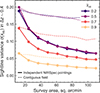 |
Fig. 14. Cosmic variance in the volume-averaged neutral fraction |


We can clearly see the impact of this cosmic variance in our sample, which covers three fields (GOODS-S, EGS and Abell 2744). For example, the majority of our z ∼ 7 − 8 spectra (8/13 sources) come from the EGS field observed by CEERS, which is known to be a large candidate ionized region (Tilvi et al. 2020; Jung et al. 2022; Tang et al. 2023; Chen et al. 2024; Napolitano et al. 2024). This is likely the cause of the high mean transmission at this redshift (Figure 8). Current results are also limited by our small sample size – this is apparent in our z ≳ 8 constraints on  , where the lack of strong damping in GNz11 lowers our
  estimate (see also, Bruton et al. 2023a): overcoming this sample variance will require tens of deep spectra. Future surveys of more sightlines could exploit the sightline variance itself, as it is related to the typical sizes of ionized regions (e.g. Lu et al. 2024).
7. Conclusions
We have investigated the redshift evolution of the Lyα break in 99 z ∼ 5.5 − 13 galaxies with publicly available JWST/NIRSpec prism spectra in the context of reionisation. We fit a sub-sample of high S/N spectra using an approach which takes into account Lyα emission, local HI absorption and IGM HI absorption using sightlines drawn from realistic inhomogeneous reionisation simulations. Our main conclusions are as follows:
-
We observe a decline in both the mean and variance of flux around the Lyα-break with increasing redshift in our sample, demonstrating strong Lyα emission is disappearing at z ≳ 7 and the spectra become increasingly ‘damped’. We find a median and 68% range of transmission is
 at z < 6, falling to
  at z > 10. We attribute this to the decreasing mean and variance in the size of ionized regions as expected in the early stages of reionisation. At z > 9, ≈80% of spectra are consistent with a neutral IGM, compared to < 40% at z < 9.
 -
We fit spectra to obtain posterior distributions for the distance of galaxies from neutral IGM, the volume-averaged IGM neutral fraction
 , and the local absorber column density NH I, for each galaxy. We find IGM properties can be reliably recovered using our approach in prism spectra with S/N≳15 per pixel, though even with the highest S/N the low resolution of the prism limits recovered distance to the neutral IGM to ≲0.5 dex. We demonstrate this can be reduced substantially with high resolution grating data.
 -
Using 14 sources with sufficient S/N we obtain posterior distributions for
 in two redshift bins. We find
  (including sightline variance) at z ≈ 6.5, 9.3 (
 excluding GNz11), providing additional evidence for a mostly neutral IGM at z > 8, consistent with independent JWST analyses of the Lyα EW distribution (Nakane et al. 2024; Tang et al. 2024c; Jones et al. 2025; Kageura et al. 2025) and galaxy damping wings (Umeda et al. 2024).
 -
Exploring local HI absorption in our sample, we find a median NH I ≈ 1020.8 cm−2, comparable to that observed in z ∼ 3 LBGs (Reddy et al. 2016), with no significant redshift evolution. At z ∼ 5.5 − 6 in GOODS-S, where our sample has high spectroscopic completeness, we find 5/6 sources which show strong DLA absorption signatures have at least one spectroscopically confirmed neighbour within r3D < 500 pkpc, compared to 6/12 for sources without DLA absorption signatures. This adds to the evidence that strong Lyα absorption may be preferentially associated with galaxies in the most massive dark matter halos (Chen et al. 2024).
The spectroscopic sensitivity and wavelength coverage of JWST/NIRSpec provide a unique opportunity to reveal the earliest stages of hydrogen reionisation. Upcoming Cycle 3 surveys (Dickinson et al. 2024; Oesch et al. 2024) are expected to obtain prism spectra of ≳100z > 10 galaxies, providing an unprecedented dataset to constrain the properties of the IGM at z ∼ 10 − 15 and infer the properties of the faint first galaxies beyond even JWST’s detection limits. Fully exploiting JWST observations to understand the early evolution of the IGM using the approach described here will require S/N ≳ 15 prism spectra and deep, high resolution follow-up studies.
Data availability
Table F.1 is available at the CDS via https://cdsarc.cds.unistra.fr/viz-bin/cat/J/A+A/705/A114
Acknowledgments
We thank Sarah Bosman, Fred Davies, Peter Jakobsen, Koki Kakiichi, Kasper Heintz, James Muzerolle, Hyunbae Park, Anne Verhamme and participants of the NORDITA workshop programme “Cosmic Dawn at High Latitudes” for useful discussions. This work is based on observations made with the NASA/ESA/CSA James Webb Space Telescope. The data were obtained from the Mikulski Archive for Space Telescopes at the Space Telescope Science Institute, which is operated by the Association of Universities for Research in Astronomy, Inc., under NASA contract NAS 5-03127 for JWST. These observations are associated with program GTO 1180, 1181, 1210, and GO 3215 (JADES; doi:10.17909/8tdj-8n28), ERS 1345 and DDT 2750 (CEERS; doi:10.17909/z7p0-8481), and GO 2561 (UNCOVER). The authors acknowledge the JADES, CEERS, and UNCOVER teams led by Daniel Eisenstein & Nora Lüetzgendorf, Steven L. Finkelstein, Pablo Arrabal Haro, and Ivo Labbé & Rachel Bezanson for developing their observing programs. CAM acknowledges support by the European Union ERC grant RISES (101163035), Carlsberg Foundation (CF22-1322), and VILLUM FONDEN (37459). Views and opinions expressed are those of the author(s) only and do not necessarily reflect those of the European Union or the European Research Council. Neither the European Union nor the granting authority can be held responsible for them. TYL acknowledges support by VILLUM FONDEN (37459). The Cosmic Dawn Center (DAWN) is funded by the Danish National Research Foundation under grant DNRF140. This work has been performed using the Danish National Life Science Supercomputing Center, Computerome.
References
- Adams, N. J., Conselice, C. J., Ferreira, L., et al. 2023, MNRAS, 518, 4755 [Google Scholar]
- Arrabal Haro, P., Dickinson, M., Finkelstein, S. L., et al. 2023, ApJ, 951, L22 [NASA ADS] [CrossRef] [Google Scholar]
- Asada, Y., Desprez, G., Willott, C. J., et al. 2025, ApJ, 983, L2 [Google Scholar]
- Asthana, S., Haehnelt, M. G., Kulkarni, G., et al. 2024, MNRAS, 533, 2843 [Google Scholar]
- Bañados, E., Venemans, B. P., Mazzucchelli, C., et al. 2018, Nature, 553, 473 [Google Scholar]
- Becker, G. D., & Bolton, J. S. 2013, MNRAS, 436, 1023 [Google Scholar]
- Begley, R., Cullen, F., McLure, R. J., et al. 2024, MNRAS, 527, 4040 [Google Scholar]
- Bezanson, R., Labbe, I., Whitaker, K. E., et al. 2024, ApJ, 974, 92 [NASA ADS] [CrossRef] [Google Scholar]
- Bolan, P., Lemaux, B. C., Mason, C., et al. 2022, MNRAS, 517, 3263 [Google Scholar]
- Bolton, J. S., & Haehnelt, M. G. 2013, MNRAS, 429, 1695 [Google Scholar]
- Bosman, S. E. I., Davies, F. B., Becker, G. D., et al. 2022, MNRAS, 514, 55 [NASA ADS] [CrossRef] [Google Scholar]
- Boyett, K., Trenti, M., Leethochawalit, N., et al. 2024, Nat. Astron., 8, 657 [CrossRef] [Google Scholar]
- Bruton, S., Lin, Y.-H., Scarlata, C., & Hayes, M. J. 2023a, ApJ, 949, L40 [NASA ADS] [CrossRef] [Google Scholar]
- Bruton, S., Scarlata, C., Haardt, F., et al. 2023b, ApJ, 953, 29 [Google Scholar]
- Bunker, A. J., Saxena, A., Cameron, A. J., et al. 2023, A&A, 677, A88 [NASA ADS] [CrossRef] [EDP Sciences] [Google Scholar]
- Bunker, A. J., Cameron, A. J., Curtis-Lake, E., et al. 2024, A&A, 690, A288 [NASA ADS] [CrossRef] [EDP Sciences] [Google Scholar]
- Cameron, A. J., Katz, H., Rey, M. P., & Saxena, A. 2023, MNRAS, 523, 3516 [NASA ADS] [CrossRef] [Google Scholar]
- Castellano, M., Fontana, A., Treu, T., et al. 2022, ApJ, 938, L15 [NASA ADS] [CrossRef] [Google Scholar]
- Chabrier, G. 2003, PASP, 115, 763 [Google Scholar]
- Chen, H. 2024, MNRAS, 528, L33 [Google Scholar]
- Chen, H., Speagle, J., & Rogers, K. K. 2023, arXiv e-prints [arXiv:2311.16238] [Google Scholar]
- Chen, Z., Stark, D. P., Mason, C., et al. 2024, MNRAS, 528, 7052 [CrossRef] [Google Scholar]
- Chevallard, J., & Charlot, S. 2016, MNRAS, 462, 1415 [NASA ADS] [CrossRef] [Google Scholar]
- Chiang, Y.-K., Overzier, R. A., Gebhardt, K., & Henriques, B. 2017, ApJ, 844, L23 [Google Scholar]
- Chisholm, J., Rigby, J. R., Bayliss, M., et al. 2019, ApJ, 882, 182 [Google Scholar]
- Christensen, L., Jakobsen, P., Willott, C., et al. 2023, A&A, 680, A82 [NASA ADS] [CrossRef] [EDP Sciences] [Google Scholar]
- Covelo-Paz, A., Giovinazzo, E., Oesch, P. A., et al. 2025, A&A, 694, A178 [NASA ADS] [CrossRef] [EDP Sciences] [Google Scholar]
- Cullen, F., McLeod, D. J., McLure, R. J., et al. 2024, MNRAS, 531, 997 [NASA ADS] [CrossRef] [Google Scholar]
- Curti, M., Witstok, J., Jakobsen, P., et al. 2025, A&A, 697, A89 [Google Scholar]
- Curtis-Lake, E., Carniani, S., Cameron, A., et al. 2023, Nat. Astron., 7, 622 [NASA ADS] [CrossRef] [Google Scholar]
- Davies, F. B., Hennawi, J. F., Bañados, E., et al. 2018, ApJ, 864, 142 [NASA ADS] [CrossRef] [Google Scholar]
- Davies, F. B., Bosman, S. E. I., Gaikwad, P., et al. 2024, ApJ, 965, 134 [NASA ADS] [CrossRef] [Google Scholar]
- Davies, F. B., Bañados, E., Hennawi, J. F., & Bosman, S. E. I. 2025, ApJ, 989, L27 [Google Scholar]
- de Belsunce, R., Gratton, S., Coulton, W., & Efstathiou, G. 2021, MNRAS, 507, 1072 [CrossRef] [Google Scholar]
- D’Eugenio, F., Maiolino, R., Carniani, S., et al. 2024, A&A, 689, A152 [NASA ADS] [CrossRef] [EDP Sciences] [Google Scholar]
- Dickinson, M., Amorin, R., Arrabal Haro, P., et al. 2024, The CANDELS-Area Prism Epoch of Reionization Survey (CAPERS), JWST Proposal. Cycle 3, ID. #6368 [Google Scholar]
- Dijkstra, M. 2014, PASA, 31 [Google Scholar]
- Dijkstra, M., Lidz, A., & Wyithe, J. S. B. 2007, MNRAS, 377, 1175 [NASA ADS] [CrossRef] [Google Scholar]
- Donnan, C. T., McLeod, D. J., Dunlop, J. S., et al. 2023, MNRAS, 518, 6011 [Google Scholar]
- Donnan, C. T., McLure, R. J., Dunlop, J. S., et al. 2024, MNRAS, 533, 3222 [NASA ADS] [CrossRef] [Google Scholar]
- Du, X., Shapley, A. E., Reddy, N. A., et al. 2018, ApJ, 860, 75 [NASA ADS] [CrossRef] [Google Scholar]
- Eilers, A.-C., Hennawi, J. F., Davies, F. B., & Oñorbe, J. 2019, ApJ, 881, 23 [NASA ADS] [CrossRef] [Google Scholar]
- Eisenstein, D. J., Johnson, B. D., Robertson, B., et al. 2023a, arXiv e-prints [arXiv:2310.12340] [Google Scholar]
- Eisenstein, D. J., Willott, C., Alberts, S., et al. 2023b, arXiv e-prints [arXiv:2306.02465] [Google Scholar]
- Endsley, R., Stark, D. P., Whitler, L., et al. 2023, MNRAS, 524, 2312 [NASA ADS] [CrossRef] [Google Scholar]
- Faucher-Giguère, C.-A., Feldmann, R., Quataert, E., et al. 2016, MNRAS, 461, L32 [CrossRef] [Google Scholar]
- Finkelstein, S. L., Bagley, M. B., Arrabal Haro, P., et al. 2022, ApJ, 940, L55 [NASA ADS] [CrossRef] [Google Scholar]
- Foreman-Mackey, D., Hogg, D. W., Lang, D., & Goodman, J. 2013, PASP, 125, 306 [Google Scholar]
- Furtak, L. J., Zitrin, A., Weaver, J. R., et al. 2023, MNRAS, 523, 4568 [NASA ADS] [CrossRef] [Google Scholar]
- Gaikwad, P., Haehnelt, M. G., Davies, F. B., et al. 2023, MNRAS, 525, 4093 [NASA ADS] [CrossRef] [Google Scholar]
- Gelli, V., Mason, C., & Hayward, C. C. 2024, ApJ, 975, 192 [NASA ADS] [CrossRef] [Google Scholar]
- Gelli, V., Mason, C., Pallottini, A., et al. 2025, A&A, submitted, [arXiv:2510.01315] [Google Scholar]
- Giarè, W., Di Valentino, E., & Melchiorri, A. 2024, Phys. Rev. D, 109, 103519 [Google Scholar]
- Greig, B., Mesinger, A., Haiman, Z., & Simcoe, R. A. 2017, MNRAS, 466, 4239 [Google Scholar]
- Greig, B., Mesinger, A., & Bañados, E. 2019, MNRAS, 484, 5094 [NASA ADS] [CrossRef] [Google Scholar]
- Greig, B., Bosman, S. E. I., Davies, F. B., et al. 2024a, MNRAS, 533, 3312 [Google Scholar]
- Greig, B., Mesinger, A., Bañados, E., et al. 2024b, MNRAS, 530, 3208 [NASA ADS] [CrossRef] [Google Scholar]
- Gunn, J. E., & Peterson, B. A. 1965, ApJ, 142, 1633 [Google Scholar]
- Hainline, K. N., D’Eugenio, F., Jakobsen, P., et al. 2024, ApJ, 976, 160 [NASA ADS] [CrossRef] [Google Scholar]
- Harikane, Y., Ouchi, M., Oguri, M., et al. 2023, ApJS, 265, 5 [NASA ADS] [CrossRef] [Google Scholar]
- Hayes, M. J., & Scarlata, C. 2023, ApJ, 954, L14 [NASA ADS] [CrossRef] [Google Scholar]
- Hayes, M., Östlin, G., Schaerer, D., et al. 2013, ApJ, 765, L27 [NASA ADS] [CrossRef] [Google Scholar]
- Hayes, M. J., Runnholm, A., Scarlata, C., Gronke, M., & Rivera-Thorsen, T. E. 2023, MNRAS, 520, 5903 [NASA ADS] [CrossRef] [Google Scholar]
- Heckman, T. M., Sembach, K. R., Meurer, G. R., et al. 2001, ApJ, 558, 56 [Google Scholar]
- Heckman, T. M., Borthakur, S., Overzier, R., et al. 2011, ApJ, 730, 5 [Google Scholar]
- Heintz, K. E., Bennett, J. S., Oesch, P. A., et al. 2024a, arXiv e-prints [arXiv:2407.06287] [Google Scholar]
- Heintz, K. E., Watson, D., Brammer, G., et al. 2024b, Science, 384, 890 [NASA ADS] [CrossRef] [Google Scholar]
- Heintz, K. E., Brammer, G. B., Watson, D., et al. 2025, A&A, 693, A60 [Google Scholar]
- Hennawi, J. F., Kist, T., Davies, F. B., & Tamanas, J. 2025, MNRAS, 539, 2621 [Google Scholar]
- Henry, A., Scarlata, C., Martin, C. L., & Erb, D. 2015, ApJ, 809, 19 [Google Scholar]
- Hu, W., Wang, J., Zheng, Z.-Y., et al. 2019, ApJ, 886, 90 [NASA ADS] [CrossRef] [Google Scholar]
- Hu, W., Martin, C. L., Gronke, M., et al. 2023, ApJ, 956, 39 [CrossRef] [Google Scholar]
- Huberty, M., Scarlata, C., Hayes, M. J., & Gazagnes, S. 2025, ApJ, 987, 82 [Google Scholar]
- Iliev, I. T., Shapiro, P. R., McDonald, P., Mellema, G., & Pen, U.-L. 2007, MNRAS, 1, 21 [Google Scholar]
- Jakobsen, P., Ferruit, P., Alves de Oliveira, C., et al. 2022, A&A, 661, A80 [NASA ADS] [CrossRef] [EDP Sciences] [Google Scholar]
- Jin, X., Yang, J., Fan, X., et al. 2023, ApJ, 942, 59 [NASA ADS] [CrossRef] [Google Scholar]
- Jones, G. C., Bunker, A. J., Saxena, A., et al. 2024, A&A, 683, A238 [NASA ADS] [CrossRef] [EDP Sciences] [Google Scholar]
- Jones, G. C., Bunker, A. J., Saxena, A., et al. 2025, MNRAS, 536, 2355 [Google Scholar]
- Jung, I., Finkelstein, S. L., Dickinson, M., et al. 2020, ApJ, 904, 144 [NASA ADS] [CrossRef] [Google Scholar]
- Jung, I., Finkelstein, S. L., Larson, R. L., et al. 2022, arXiv e-prints [arXiv:2212.09850] [Google Scholar]
- Jung, I., Finkelstein, S. L., Arrabal Haro, P., et al. 2024, ApJ, 967, 73 [NASA ADS] [CrossRef] [Google Scholar]
- Kageura, Y., Ouchi, M., Nakane, M., et al. 2025, ApJS, 278, 33 [Google Scholar]
- Kakiichi, K., & Gronke, M. 2021, ApJ, 908, 30 [CrossRef] [Google Scholar]
- Kalberla, P. M. W., & Kerp, J. 2009, ARA&A, 47, 27 [NASA ADS] [CrossRef] [Google Scholar]
- Katz, H., Cameron, A. J., Saxena, A., et al. 2025, Open J. Astrophys., 8, 104 [Google Scholar]
- Keating, L. C., Weinberger, L. H., Kulkarni, G., et al. 2020, MNRAS, 491, 1736 [NASA ADS] [CrossRef] [Google Scholar]
- Keating, L. C., Bolton, J. S., Cullen, F., et al. 2024a, MNRAS, 532, 1646 [Google Scholar]
- Keating, L. C., Puchwein, E., Bolton, J. S., Haehnelt, M. G., & Kulkarni, G. 2024b, MNRAS, 531, L34 [Google Scholar]
- Kimm, T., Blaizot, J., Garel, T., et al. 2019, MNRAS, 486, 2215 [Google Scholar]
- Kist, T., Hennawi, J. F., & Davies, F. B. 2025a, MNRAS, [arXiv:2504.14746] [Google Scholar]
- Kist, T., Hennawi, J. F., & Davies, F. B. 2025b, MNRAS, 538, 2704 [Google Scholar]
- Krogager, J. K., De Cia, A., Heintz, K. E., et al. 2024, MNRAS, 535, 561 [Google Scholar]
- Larson, R. L., Finkelstein, S. L., Hutchison, T. A., et al. 2022, ApJ, 930, 104 [NASA ADS] [CrossRef] [Google Scholar]
- Laursen, P., Sommer-Larsen, J., & Andersen, A. C. 2009, ApJ, 704, 1640 [Google Scholar]
- Laursen, P., Sommer-Larsen, J., & Razoumov, A. O. 2011, ApJ, 728, 52 [Google Scholar]
- Lidz, A., Chang, T.-C., Mas-Ribas, L., & Sun, G. 2021, ApJ, 917, 58 [NASA ADS] [CrossRef] [Google Scholar]
- Lu, T.-Y., Mason, C. A., Hutter, A., et al. 2024, MNRAS, 528, 4872 [CrossRef] [Google Scholar]
- Ma, X., Quataert, E., Wetzel, A., et al. 2020, MNRAS, 498, 2001 [Google Scholar]
- Madau, P., Haardt, F., & Rees, M. J. 1999, ApJ, 514, 648 [CrossRef] [Google Scholar]
- Mason, C. A., & Gronke, M. 2020, MNRAS, 499, 1395 [Google Scholar]
- Mason, C. A., Trenti, M., & Treu, T. 2015, ApJ, 813, 21 [NASA ADS] [CrossRef] [Google Scholar]
- Mason, C. A., Treu, T., de Barros, S., et al. 2018a, ApJ, 857, L11 [Google Scholar]
- Mason, C. A., Treu, T., Dijkstra, M., et al. 2018b, ApJ, 856, 2 [Google Scholar]
- Mason, C. A., Fontana, A., Treu, T., et al. 2019, MNRAS, 485, 3947 [NASA ADS] [CrossRef] [Google Scholar]
- Mason, C. A., Naidu, R. P., Tacchella, S., & Leja, J. 2019, MNRAS, 489, 2669 [Google Scholar]
- Mason, C. A., Trenti, M., & Treu, T. 2023, MNRAS, 521, 497 [NASA ADS] [CrossRef] [Google Scholar]
- McGreer, I. D., Mesinger, A., & D’Odorico, V. 2015, MNRAS, 447, 499 [NASA ADS] [CrossRef] [Google Scholar]
- McQuinn, M., Lidz, A., Zahn, O., et al. 2007, MNRAS, 377, 1043 [Google Scholar]
- McQuinn, M., Lidz, A., Zaldarriaga, M., Hernquist, L., & Dutta, S. 2008, MNRAS, 388, 1101 [NASA ADS] [Google Scholar]
- Mesinger, A., & Furlanetto, S. 2007, ApJ, 669, 663 [Google Scholar]
- Mesinger, A., & Furlanetto, S. R. 2008, MNRAS, 385, 1348 [NASA ADS] [CrossRef] [Google Scholar]
- Mesinger, A., Aykutalp, A., Vanzella, E., et al. 2015, MNRAS, 446, 566 [Google Scholar]
- Mesinger, A., Greig, B., & Sobacchi, E. 2016, MNRAS, 459, 2342 [NASA ADS] [CrossRef] [Google Scholar]
- Meyer, R. A., Oesch, P. A., Giovinazzo, E., et al. 2024, MNRAS, 535, 1067 [CrossRef] [Google Scholar]
- Meyer, R. A., Roberts-Borsani, G., Oesch, P. A., & Ellis, R. S. 2025, MNRAS, 542, 1952 [Google Scholar]
- Miralda-Escude, J. 1998, ApJ, 501, 15 [CrossRef] [Google Scholar]
- Morales, A. M., Mason, C. A., Bruton, S., et al. 2021, ApJ, 919, 120 [CrossRef] [Google Scholar]
- Morales, A. M., Finkelstein, S. L., Leung, G. C. K., et al. 2024, ApJ, 964, L24 [NASA ADS] [CrossRef] [Google Scholar]
- Morishita, T., Roberts-Borsani, G., Treu, T., et al. 2023, ApJ, 947, L24 [NASA ADS] [CrossRef] [Google Scholar]
- Morishita, T., Stiavelli, M., Chary, R.-R., et al. 2024, ApJ, 963, 9 [NASA ADS] [CrossRef] [Google Scholar]
- Mortlock, D. J., Warren, S. J., Venemans, B. P., et al. 2011, Nature, 474, 616 [Google Scholar]
- Naidu, R. P., Oesch, P. A., van Dokkum, P., et al. 2022, arXiv e-prints [arXiv:2207.09434] [Google Scholar]
- Nakane, M., Ouchi, M., Nakajima, K., et al. 2024, ApJ, 967, 28 [NASA ADS] [CrossRef] [Google Scholar]
- Napolitano, L., Pentericci, L., Santini, P., et al. 2024, A&A, 688, A106 [NASA ADS] [CrossRef] [EDP Sciences] [Google Scholar]
- Nasir, F., Cain, C., D’Aloisio, A., Gangolli, N., & McQuinn, M. 2021, ApJ, 923, 161 [Google Scholar]
- Oesch, P. A., Brammer, G., Naidu, R. P., et al. 2023, MNRAS, 525, 2864 [NASA ADS] [CrossRef] [Google Scholar]
- Oesch, P., Naidu, R., Atek, H., et al. 2024, Mirage or Miracle? Spectroscopic Confirmation of Remarkably Luminous Galaxies at z>10, JWST Proposal. Cycle 3, ID. #5224 [Google Scholar]
- Ouchi, M., Harikane, Y., Shibuya, T., et al. 2017, PASJ, 00, 1 [Google Scholar]
- Pagano, L., Delouis, J. M., Mottet, S., Puget, J. L., & Vibert, L. 2020, A&A, 635, A99 [NASA ADS] [CrossRef] [EDP Sciences] [Google Scholar]
- Pahl, A. J., Shapley, A., Faisst, A. L., et al. 2020, MNRAS, 493, 3194 [Google Scholar]
- Park, H., Jung, I., Song, H., et al. 2021, ApJ, 922, 263 [NASA ADS] [CrossRef] [Google Scholar]
- Park, H., Jung, I., Yajima, H., et al. 2025, ApJ, 983, 91 [Google Scholar]
- Pei, Y. C. 1992, ApJ, 395, 130 [Google Scholar]
- Pentericci, L., Vanzella, E., Fontana, A., et al. 2014, ApJ, 793, 113 [NASA ADS] [CrossRef] [Google Scholar]
- Pérez-González, P. G., Costantin, L., Langeroodi, D., et al. 2023, ApJ, 951, L1 [CrossRef] [Google Scholar]
- Planck Collaboration VI. 2020, A&A, 641, A6 [NASA ADS] [CrossRef] [EDP Sciences] [Google Scholar]
- Prieto-Lyon, G., Mason, C., Mascia, S., et al. 2023, ApJ, 956, 136 [NASA ADS] [CrossRef] [Google Scholar]
- Qin, Y., Mesinger, A., Prelogović, D., et al. 2025, PASA, 42 [Google Scholar]
- Rahmati, A., Schaye, J., Bower, R. G., et al. 2015, MNRAS, 452, 2034 [CrossRef] [Google Scholar]
- Reddy, N. A., Steidel, C. C., Pettini, M., Bogosavljević, M., & Shapley, A. E. 2016, ApJ, 828, 108 [Google Scholar]
- Ren, K., Trenti, M., & Mason, C. A. 2019, ApJ, 878, 114 [Google Scholar]
- Rieke, M. J., Robertson, B., Tacchella, S., et al. 2023, ApJS, 269, 16 [NASA ADS] [CrossRef] [Google Scholar]
- Rivera-Thorsen, T. E., Hayes, M., Östlin, G., et al. 2015, ApJ, 805, 14 [Google Scholar]
- Robertson, B., Johnson, B. D., Tacchella, S., et al. 2024, ApJ, 970, 31 [NASA ADS] [CrossRef] [Google Scholar]
- Rudie, G. C., Steidel, C. C., Trainor, R. F., et al. 2012, ApJ, 750, 67 [NASA ADS] [CrossRef] [Google Scholar]
- Santos, M. R. 2004, MNRAS, 349, 1137 [NASA ADS] [CrossRef] [Google Scholar]
- Saxena, A., Bunker, A. J., Jones, G. C., et al. 2024, A&A, 684, A84 [NASA ADS] [CrossRef] [EDP Sciences] [Google Scholar]
- Scarlata, C., & Panagia, N. 2015, ApJ, 801, 43 [Google Scholar]
- Schenker, M. A., Ellis, R. S., Konidaris, N. P., & Stark, D. P. 2014, ApJ, 795, 20 [NASA ADS] [CrossRef] [Google Scholar]
- Shapley, A. E., Steidel, C. C., Pettini, M., & Adelberger, K. L. 2003, ApJ, 588, 65 [Google Scholar]
- Sheth, R. K., Mo, H. J., & Tormen, G. 2001, MNRAS, 323, 1 [NASA ADS] [CrossRef] [Google Scholar]
- Sobacchi, E., & Mesinger, A. 2014, MNRAS, 440, 1662 [NASA ADS] [CrossRef] [Google Scholar]
- Sobacchi, E., & Mesinger, A. 2015, MNRAS, 453, 1843 [Google Scholar]
- Stark, D. P., Ellis, R. S., Chiu, K., Ouchi, M., & Bunker, A. 2010, MNRAS, 408, 1628 [Google Scholar]
- Steidel, C. C., Erb, D. K., Shapley, A. E., et al. 2010, ApJ, 717, 289 [Google Scholar]
- Stern, J., Sternberg, A., Faucher-Giguère, C.-A., et al. 2021, MNRAS, 507, 2869 [NASA ADS] [CrossRef] [Google Scholar]
- Tacchella, S., McClymont, W., Scholtz, J., et al. 2025, MNRAS, 540, 851 [Google Scholar]
- Tang, M., Stark, D. P., Chen, Z., et al. 2023, MNRAS, 526, 1657 [NASA ADS] [CrossRef] [Google Scholar]
- Tang, M., Stark, D. P., Ellis, R. S., et al. 2024a, MNRAS, 531, 2701 [NASA ADS] [CrossRef] [Google Scholar]
- Tang, M., Stark, D. P., Ellis, R. S., et al. 2024b, ApJ, 972, 56 [NASA ADS] [CrossRef] [Google Scholar]
- Tang, M., Stark, D. P., Topping, M. W., Mason, C., & Ellis, R. S. 2024c, ApJ, 975, 208 [NASA ADS] [CrossRef] [Google Scholar]
- Tanvir, N. R., Fynbo, J. P. U., Postigo, A. d. U., et al. 2019, MNRAS, 483, 5380 [Google Scholar]
- Tasitsiomi, A. 2006, ApJ, 645, 792 [NASA ADS] [CrossRef] [Google Scholar]
- Taylor, J., & Lidz, A. 2014, MNRAS, 437, 2542 [NASA ADS] [CrossRef] [Google Scholar]
- Terp, C., Heintz, K. E., Watson, D., et al. 2024, A&A, 690, A70 [NASA ADS] [CrossRef] [EDP Sciences] [Google Scholar]
- Tilvi, V., Malhotra, S., Rhoads, J. E., et al. 2020, ApJ, 891, L10 [NASA ADS] [CrossRef] [Google Scholar]
- Topping, M. W., Stark, D. P., Endsley, R., et al. 2024, MNRAS, 529, 4087 [NASA ADS] [CrossRef] [Google Scholar]
- Tortora, L., Feldmann, R., Bernardini, M., & Faucher-Giguère, C.-A. 2024, MNRAS, 532, 3847 [Google Scholar]
- Trainor, R. F., Strom, A. L., Steidel, C. C., et al. 2019, ApJ, 887, 85 [NASA ADS] [CrossRef] [Google Scholar]
- Turner, M. L., Schaye, J., Crain, R. A., et al. 2017, MNRAS, 471, 690 [NASA ADS] [CrossRef] [Google Scholar]
- Umeda, H., Ouchi, M., Nakajima, K., et al. 2024, ApJ, 971, 124 [NASA ADS] [CrossRef] [Google Scholar]
- Umeda, H., Ouchi, M., Kageura, Y., et al. 2025a, arXiv e-prints [arXiv:2504.04683] [Google Scholar]
- Umeda, H., Ouchi, M., Kikuta, S., et al. 2025b, ApJS, 277, 37 [Google Scholar]
- van de Voort, F., Springel, V., Mandelker, N., van den Bosch, F. C., & Pakmor, R. 2019, MNRAS, 482, L85 [NASA ADS] [CrossRef] [Google Scholar]
- Verhamme, A., Orlitová, I., Schaerer, D., & Hayes, M. 2015, A&A, 578, A7 [NASA ADS] [CrossRef] [EDP Sciences] [Google Scholar]
- Wang, F., Davies, F. B., Yang, J., et al. 2020, ApJ, 896, 23 [NASA ADS] [CrossRef] [Google Scholar]
- Weaver, J. R., Cutler, S. E., Pan, R., et al. 2024, ApJS, 270, 7 [NASA ADS] [CrossRef] [Google Scholar]
- Weinberger, L. H., Haehnelt, M. G., & Kulkarni, G. 2019, MNRAS, 485, 1350 [NASA ADS] [CrossRef] [Google Scholar]
- Whitler, L. R., Mason, C. A., Ren, K., et al. 2020, MNRAS, 495, 3602 [Google Scholar]
- Whitler, L., Stark, D. P., Topping, M. W., et al. 2025, ApJ, 992, 63 [Google Scholar]
- Wisotzki, L., Bacon, R., Blaizot, J., et al. 2016, A&A, 587, A98 [NASA ADS] [CrossRef] [EDP Sciences] [Google Scholar]
- Witstok, J., Jakobsen, P., Maiolino, R., et al. 2025, Nature, 639, 897 [Google Scholar]
- Yang, J., Wang, F., Fan, X., et al. 2020, ApJ, 897, L14 [Google Scholar]
- Yang, L., Morishita, T., Leethochawalit, N., et al. 2022, ApJ, 938, L17 [NASA ADS] [CrossRef] [Google Scholar]
Assuming a spherically symmetric bubble of radius Rb and galaxies uniformly distributed inside the bubble  .
.
At the time of writing there are 11 additional sources in the public archive from Cycle 1+2 with S/N > 15, but all are z < 7.7. As our focus is the earliest stages of reionisation at z ≳ 9 we leave analysis of these lower redshift sources to future work.
Given the resolution of the prism at 1 μm (Δz ≳ 0.05, ≳100 pkpc) this can be due to an unresolved ensemble of absorbers, thus we use the subscript eff to denote it is an effective optical depth, and add a single absorber at the redshift of the source.
We calculate the line spread function using observations from CAL-1125 of a planetary nebula IRAS-05248-7007 in the LMC. We find R ∼ 45 around ∼1 μm.
Where N is the number of spectral pixels we fit over.
We note NH I can be sensitive to the continuum model, e.g. using a power-law fit to the > 1400 Å continuum can result in ∼1 dex higher NH I than using the BEAGLE continuum model. As described in Section 4, photoionization models should provide better fits to the UV continuum compared to power-law fits as they include nebular continuum.
Appendix A: Comparison with analytic damping wings
As described in Section 2 there is significant sightline variance in the IGM during reionisation, thus the assumption of a uniform IGM can bias the recovery of  , as the relationship between
  , Db and the transmission is not deterministic. This has been previously discussed in detail by Mesinger & Furlanetto (2008) and we demonstrate this effect with our simulations here.
For every galaxy in our grid of simulations spanning xHI ∈ [0,1] at z = 9, we calculate the distance to the first neutral region, Db, and the Lyα transmission 200 km/s redward of Lyα line centre from the IGM damping wing (calculated over each galaxy’s sightline as described in Section 2.1). In the top panel of Figure A.1 we plot the median transmission at +200 km/s redward of Lyα, taking the median of galaxies in bins of Db, as a function of  . In the lower panel we plot the Lyα transmission 200 km/s redward of Lyα line centre predicted by the Miralda-Escude (1998) uniform IGM approximation, also as a function of Db and
  . We also show the mean bubble size predicted in the simulations as a function of
  . The transmission obtained from the inhomogeneous IGM simulations demonstrates the damping wing optical depth depends most strongly on Db, with little dependence on
  (see also, Mesinger & Furlanetto 2008; Chen 2024; Keating et al. 2024b).
We see the uniform IGM approximation works least well when both  and Db are low,
  , and Db < 30 cMpc. Under the uniform IGM assumption, a galaxy a short distance from a neutral patch in a mostly ionized IGM is predicted to have very high transmission ∼100%, as the approximation assumes the neutral patch is ≪100% neutral, decreasing its optical depth, when in reality the optical depth should be higher. The uniform IGM approximation will thus overpredict Lyα transmission in this case, and thus lead to overestimates in
  . The sensitivity of the damping wing transmission to the distance of galaxies to neutral gas is clear motivation for using a realistic IGM simulation as a prior for
  . At a given redshift, the inferred distribution of Db provides information about
  .
.
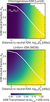 |
Fig. A.1. Lyman-alpha damping wing transmission at Δv = 200 km/s as a function of the distance of a galaxy from the nearest neutral patch and the IGM mean neutral fraction |


Appendix B: Transmission profiles
Here we describe some additional effects which impact Lyα transmission profiles, illustrated at the resolution of NIRSpec prism and G140M grating in Figure B.1: (1) the HI column density NH I; (2) the covering fraction of local HI fcov; (3) a proximate absorber along the line of sight; and (4) galaxies for which a precise spectroscopic redshift cannot be measured from emission lines. In all plots the grey solid line shows the input mock spectrum at z = 10 without any attenuation from DLAs or the IGM.
The top panel of Figure B.1 shows the impact of local HI absorbers both with and without attenuation from the neutral IGM (thick vs thin lines) as a function of NH I (coloured lines). At fixed NH I, the neutral IGM produces more attenuation at redder wavelengths than local absorbers alone, meaning these can be distinguished with sufficient S/N and resolution.
The second panel shows the transmission due to local HI gas, including a non-uniform covering fraction fcov. In this case the transmission is given by (e.g. Rivera-Thorsen et al. 2015)
 (B.1)
(B.1)
where τDLA is given by Equation 4. Here we show an example with NH I = 1022 cm−2, applying a fully neutral IGM to the damped cases. Reducing the covering fraction increases the transmitted flux redward of Lyα line centre.
The third panel also shows a NH I = 1022 cm−2 local absorber, but where the absorbing gas is not located in the emitting source but has a peculiar velocity, ΔvDLA, which also increases transmission redward of Lyα line centre. At the resolution of the prism, cases with non-zero covering fraction, fcov ∼ 0.5 and large peculiar velocities, ΔvDLA ∼ −5000 km/s, can produce very similar spectra, introducing a degeneracy. As discussed in Section 6.2 we consider the local non-uniform covering fraction a likely more physical picture of the local absorption.
In the bottom row of Figure B.1 we show that even without a precise spectroscopic redshift from emission lines it should still be possible to get information about the IGM, but that there is a degeneracy between NH I and redshift. We show that at the resolution of the NIRSpec prism, in a fully neutral IGM, a source at redshift zspec with a local absorber column density of log10NH I ≲ 21 has an almost identical transmission profile to a source with log10NH I ≲ 20 but at z ≈ zspec + 0.05. This is because the DLA removes flux very close to line center. However, as the neutral IGM reduces the flux at > 1240 Å more strongly than the DLA, we should still be able to recover some information about the IGM in either case (i.e. the coloured lines are significantly different from the grey line). This means we are still able to use sources at z > 10, even without a spectroscopic redshift determination from e.g. [OIII] emission lines.
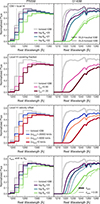 |
Fig. B.1. Example spectra (fλ), convolved to the resolution of the NIRSpec prism (upper panels) and G140M grating (lower panels), showing the impact of a non-uniform covering fraction of local absorbers, fcov (left panels); if the absorber is located at a lower redshift than the emitting source, but with a peculiar velocity, ΔvDLA towards the source (central panels); and if the source is at a slightly higher redshift than the estimated zspec (right panels; i.e. if the redshift can only be measured from the break, not emission lines), highlighting some of the degeneracies between these effects at the resolution of the prism. |
Appendix C: Evolution of stacked spectra
To gain intuition into the redshift evolution of stacked spectra (Figure 6) we explore four simple physically motivated models. Because of the low resolution of the prism, this requires using high-resolution R ≳ 1000 spectral templates, applying the models, and then convolving with the prism resolution. As no R > 1000 templates for the faint z ∼ 5 − 6 galaxies in our sample exist yet, we construct them from fits to our z < 6 sample as described in Section 4, naturally including any local absorption in the ISM and CGM of galaxies at z ∼ 5.5 − 6. We take samples from the posteriors for each z < 6 galaxy (29 galaxies) to generate template spectra with a resolution of R ∼ 4000 to which we can apply transmission models.
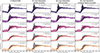 |
Fig. C.1. Median stacked spectra in redshift bins as in Figure 6. At z < 6 (top panel) we show the median and 68% range of our template spectra in a fully ionized IGM, convolved to the prism resolution (grey line and shaded region). At z ≥ 6 we show the predicted median and 68% range of spectra assuming four IGM/CGM evolution models (grey line and shaded region, described in Appendix C): (1) an increasingly neutral IGM following the Mason et al. (2019) reionisation history; (2) DLA column densities increase with increase cosmic density, NH I ∝ (1+z)2; (3) the same density evolution and at z > 6 a minimum log10NH I > 20.3 due to the lower UV background; (4) assuming the same density evolution and that fcov = 1 at z > 6. The spectra are most consistent with the majority of the evolution being driven by the IGM evolution. |
We show the median and 68% range of these templates, normalised and convolved to the resolution of the prism, as the grey line and shaded region in the top panels of Figure C.1. We then apply four simple models and describe their predictions for the evolution of the spectra:
-
Neutral IGM: We apply damping wings drawn from our IGM simulations (Section 2.1.1) to the templates, assuming
 predicted by Mason et al. (2019). This model predicts a decrease in both the mean flux and variance around Lyα as ionized regions become too rare and small to transmit significant flux (e.g. Mason et al. 2018a). In Figure C.1, we see our stacks agree qualitatively very well with this model.
 -
Local absorber density evolution: Assuming DLA column density increases with increasing cosmic density, NH I ∝ (1+z)2. This assumes that most of the evolution is due to an increase in density in the CGM, and that the CGM is mostly neutral at z ∼ 6 (as predicted by some hydrodynamic simulations, e.g. Stern et al. 2021). This model predicts it would still be possible to observe strong Lyα emission at z > 8, producing spectra which are inconsistent with the observations at z > 8 where we do not detect strong Lyα emission. This is because at z < 6 many spectra require low column densities (NH I < 1019 cm−2) to explain the strong Lyα emission in this bin, and the (1 + z)2 evolution will not produce enough opacity to significantly damp Lyα in all sources at z > 8. Thus we do not consider pure density evolution in the CGM a primary driver of the observed evolution in the prism spectra.
-
UV background evolution: Assuming an increase in LLS and sub-DLAs (17.2 < log10NH I < 20.3), within ionized regions at z ≳ 6 as the UV background drops before ionized regions merge (as predicted by hydrodynamical simulations Bolton & Haehnelt 2013; Rahmati et al. 2015; Nasir et al. 2021). To explore this we impose a minimum log10NH I > 20.3 in the local absorber model, but note this likely overestimates the importance of absorbers. This model is also not a good match to the observations for two reasons: firstly, the evolution in self-shielded systems is expected to occur rapidly at the end of reionisation (e.g. Nasir et al. 2021), so we would expect a sharp increase in absorption systems with redshift at z ≳ 6. In our data we see strong Lyα emission at z ∼ 5 − 7, implying the spectra cannot be fully explained by a rapid evolution in self-shielding systems at the end of reionisation. Secondly, the predicted continuum in this model at z > 8 is higher than the observed spectra, as not all sources have high enough column densities to significantly damp the continuum, implying additional neutral IGM attenuation is still needed (see Figure 4).
-
Covering fraction evolution: We assume an extreme model where the covering fraction of local HI fcov = 1 at z > 6. This is motivated by some hydrodynamical simulations showing an increase in covering fractions in the CGM with increasing redshift (Rahmati et al. 2015; Tortora et al. 2024). However, we note fcov depends strongly on feedback prescriptions and resolution in simulations (Faucher-Giguère et al. 2016; van de Voort et al. 2019). This model underpredicts the observed spectra at z ∼ 6 − 7 (because it predicts strong Lyα is all absorbed), but overpredicts the observed spectra at z > 8 (for the same reason as in the UVB evolution case). A gradual increase in fcov with redshift could contribute to some of the observed evolution of the stacks. We discuss this further in Section 6.2.
Thus we conclude that, while local absorption is present in the observed spectra over all redshifts, the observations are most consistent with the majority of the redshift evolution being driven by the neutral IGM evolution.
Appendix D: Bayesian inference setup and priors
We use Bayesian inference to infer the parameters  , Db and θgal (=θLyα, θDLA) for each galaxy. For z > 10 sources without spectroscopic redshifts from emission lines we also fit for zspec, using a Gaussian prior for the redshift based on an initial fit to the Lyα break. The posterior for each galaxy, with observed spectrum fi, obs and properties ϕgal, i (MUV, OIII+Hβ EW) is
 (D.1)
(D.1)
Here  is the likelihood (Equation 7) as described in Section 4.
We use a conditional prior  from our simulations (Section 2.1.1), selecting sightlines based on MUV to account for brighter galaxies being more likely to be in larger bubbles (step 5 above, Mason et al. 2018a, though this does not have a large impact on our results). Using this prior makes the inference of
  for each galaxy explicitly conditional on Db, thereby propagating uncertainties in the inferred Db values into the uncertainties on
  . As the damping wings are relatively independent of
  at fixed Db (see Appendix A), the redshift evolution of Db should provide the most empirical evidence for IGM evolution, regardless of the mapping to xHI. At z ≤ 6.3 we use half-Gaussian priors on
  based on the Lyα+β forest dark pixel fraction constraints by Jin et al. (2023). At higher redshifts we assume a uniform prior on
 ![Mathematical equation: $ \overline{x}_{{\small { {\text{HI}}}}}=[0,1] $](/articles/aa/full_html/2026/01/aa53820-25/aa53820-25-eq152.gif) .
.
We use the empirical distributions of Lyα EW by Tang et al. (2024a) as a prior on the emergent Lyα EW (i.e. after transmission through the ISM and CGM, calculated after step 4 above), such that at z ∼ 5 − 6 we should recover the observed Lyα EW distribution, and at z > 6 the observed EW distribution does not exceed that at z ∼ 5 − 6 (which is reasonable based on NIRSpec grating and ground-based spectra, e.g. Pentericci et al. 2014; Mason et al. 2019; Jung et al. 2020; Tang et al. 2024c). These distributions are derived from > 700 z ∼ 5 − 6 Lyman-break galaxies with ground-based Lyα spectroscopy from Keck and JWST photometry. Due to the high resolution (R ∼ 4000) of the ground-based spectroscopy, these EW measurements will not be impacted by local absorption, unlike in the prism where Lyα emission and local absorption are blended. Thus, this prior should be informative for recovering the NH I distribution from the prism. For sources at z ≲ 10, where [OIII]+Hβ is detectable in NIRCam and NIRSpec, we use the EW model by Tang et al. (2024a) conditional on [OIII]+Hβ EW (whereby sources with strong [OIII]+Hβ EW are more likely to have strong Lyα). For sources without [OIII]+Hβ measurements we use the EW distribution conditional on MUV. Following Tang et al. (2024a) we apply a slit-loss correction of 0.8 to map predicted Lyα fluxes based on VLT/MUSE measurements to the NIRSpec slits. Similarly, we use the Lyα velocity offsets model by Mason et al. (2018b) as a prior on the emergent velocity offset. We use a uniform prior on log10NH I ∈ [17,23.5], noting that for log10NH I/cm−2 ≲ 20, unless there is strong Lyα emission, at the resolution of the prism we can only obtain an upper limit on NH I (see Figure 4). Motivated by z ∼ 3 results by Reddy et al. (2016) which imply HI covering fractions in the ISM are high (≳90%), we use a prior which is uniform in log(1 − fcov): p(fcov) = 1/(1 − fcov + ϵ). This avoids non-physical scenarios with very high NH I and low fcov.
We obtain the posterior for each galaxy,  using Markov chain Monte Carlo with the emcee sampler (Foreman-Mackey et al. 2013). We fit over the rest-frame wavelength range 1100 − 1400 Å, which we find provides the most robust recovery of parameters in mock spectra, and contains no other UV emission lines except NV which is expected to be very weak for stellar populations ≳5 Myr (Chisholm et al. 2019). We use 50 walkers and ∼104 − 5 steps, such that the chain is > 50× the integrated autocorrelation time for the number of fitted parameters, and discard the first 50% of the chain. To obtain the marginalised
  we take the resulting
  samples from each galaxy and fit a smooth function with a Gaussian Kernel Density Estimation. The final posterior of
  at a given redshift is then the product of the individual
  posteriors in each bin (Section 5.2). In Figure D.1 we show the individual
  posteriors for the 14 S/N> 15 galaxies in our sample, in two redshift bins (see Section 5.2), and their combined posterior.
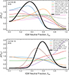 |
Fig. D.1. Neutral fraction, |

Appendix E: Validation of fitting
We validate our fits using mock data and describe our key results here. As described in Sections 2.1 and 6.3, and Appendix A, the IGM damping wing optical depth depends most strongly on Db, and so by essentially estimating the distribution of Db at a given redshift, we can map to  (Figure 2, see also e.g. Kist et al. 2025a). Thus, we first demonstrate what S/N per pixel is required to robustly recover the most important parameters – Db and NH I. We then show an example of fitting a high S/N mock prism spectrum showing the recovery of the other parameters. In Section 6.3 we investigate how many sources are required to accurately recover
  to ≲0.2.
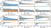 |
Fig. E.1. Accuracy of recovered distance to neutral IGM, Db, and local column density, NH I as a function of S/N per pixel in mock NIRSpec prism and G140M observations. We show the median and 68% range of the maximum likelihood recovered values from 100 realisations. The low resolution of the prism limits the accuracy of constraints, while robust constraints could be obtained even for low S/N (∼5 per pixel) with G140M. |
We generate mock spectra from the BEAGLE fits to our sample as templates, and apply IGM damping wings and DLA optical depths on a grid of Db and NH I values. We then add noise, accounting for the covariance between adjacent pixels (Equation 8), to the model spectra and fit the spectra using the approach described in Section 4, verifying that input parameters can be recovered well for high S/N spectra.
We demonstrate the impact of S/N on our parameter recovery in Figure E.1. This shows the median and 68% range of the maximum likelihood recovered values of distance to neutral IGM, Db, and local column density, NH I as a function of S/N per pixel, from mock spectra. For each S/N value we generate 100 realisations of the flux given the covariance matrix (obtained by rescaling the observed error spectrum for our template source). We show the recovered parameters for 6 input combinations of Db = [1, 10, 100] cMpc and log10NH I = [19,21] for both mock prism observations and G140M observations.
Figure E.1 demonstrates that IGM and DLA properties can be robustly recovered from prism spectra, but that there can be large uncertainties in parameters recovered from prism spectra, even for very high S/N spectra (∼0.5 dex for S/N∼50 spectra). This is due to the low resolution, limiting our ability to distinguish small changes in the shape of the continuum. By contrast, G140M observations promise to provide precise constraints on both Db and NH I for spectra with S/N≳5.
We see S/N≳15 is required to robustly recover the input Db from prism spectra, and that for small input bubble sizes, there can be a bias to larger bubble sizes and higher NH I with low S/N spectra. This is because the shape of the damping wing is mostly insensitive to Db ≲ 5 cMpc (see Figure 3), so negative noise fluctuations will not significantly shift the inferred Db lower, while positive noise fluctuations will always result in a higher inferred Db. Future work could potentially mitigate this bias by e.g. modifying the likelihood form or using machine learning approaches (Chen et al. 2023; Park et al. 2025). This bias is not present in grating observations due to the higher resolution around the break. We find NH I can be recovered well, to within ≲0.2 dex, for S/N≳5 per pixel in both prism and grating spectra. We note that the shape of the damping wing in the continuum as seen in prism is mostly insensitive to NH I ≲1020 cm−2, so in those cases we only return upper limits.
In Figure E.2 we show an example of the recovered posteriors from fitting a mock spectrum. For this example we apply IGM damping wings (using a simulated sightline at  with Db = 5 cMpc), a DLA with log10NH I = 21.0 and fcov = 1, and an emergent Lyα emission line (i.e. pre-IGM absorption) with EW = 30 Å, Δv = FWHM = 200 km/s. We add uncertainties to the spectrum assuming S/N = 50 per pixel. We see all input parameters can be recovered well within 2σ, though the uncertainties are large, as expected from Figure E.1. This figure demonstrates there is some degeneracy between NH I and Db, and between NH I and fcov, but that a low Db ≲ 20 cMpc can be clearly recovered even when NH I is high (> 1021 cm−2). We see
  is the least well-recovered parameter. As described in Section 2.1, our recovery of
  depends on estimating the distribution of Db at a given redshift, so our recovered
  depends on our prior
  . In this example, we see we recover
  . This is consistent with the expectation from Figure 2 that 5 cMpc bubbles are most common when
  . This highlights how observations of multiple galaxies are required to overcome the sightline variance in the IGM and accurately recover
  at a given redshift. We explore this more quantitively in Section 6.3.
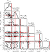 |
Fig. E.2. Recovered posteriors for an example mock prism spectrum with S/N = 50 per pixel. All input parameters (shown as red crosshairs) are recovered well within 2σ. Our constraint on |


Appendix F: Sample and spectra
In Table F.1 (available at the CDS) we list IDs, coordinates, spectroscopic redshifts and MUV for our sample. In Figures F.1-F.4 we show the individual prism spectra (black) and error spectrum (grey shaded region). The median BEAGLE fit to the spectrum is shown in orange over the region we fit to (> 1500 Å in the rest-frame) and in blue in the region where we do not fit – which represents the predicted unattenuated continuum which we use to fit the damping wings (Section 4). Smaller panels show a zoomed region around the Lyα break, showing the observed spectra, median BEAGLE continuum prediction assuming ionized IGM (thick blue line) and fully neutral IGM (thin blue line), and the best-fit damping wing model (red line and shaded region marking median and 68% range of samples of the posterior).
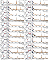 |
Fig. F.1. Spectra of our sample in ascending redshift order. We show the NIRSpec prism spectra in black with the error spectrum in shaded grey. The best-fit BEAGLE model is shown in orange, convolved to the prism resolution. The blue lines are the extrapolation of the BEAGLE model to the rest-frame < 1500 Å, which is the predicted continuum spectrum we use for our damping wing fits (Section 4). Small panels show the damping wing fit zoomed in around 1100-1400 Å in the rest-frame (marked as the red shaded region on the full spectra). The thick blue lines show the BEAGLE continuum model extrapolation in an ionized IGM, the thin blue lines show the continuum model assuming a fully neutral IGM with no ionized bubble around the source. The red line and shaded region showing median and 68% range of samples from posteriors. |
All Figures
|
Fig. 1. Top panels: Example 300 cMpc × 300 cMpc slices of the ionization field (white patches show ionized gas, black neutral gas) in our (1.6 cGpc)3 simulations at |
| In the text | |
|
Fig. 2. Median, 68% and 95% range of distances of MUV ∼ −19.3 galaxies (the median in our sample) to the neutral IGM, Db as a function of |
| In the text | |
|
Fig. 3. Mock spectra at z = 10 demonstrating the impact of the distance from neutral IGM, Db. Left (right) panels show the spectrum convolved to the resolution of the NIRSpec prism (G140M grating). The grey line shows the spectrum in an almost fully ionized IGM (i.e. Lyα is attenuated only blueward of resonance by the Gunn & Peterson (1965) optical depth). Coloured lines show the spectrum if the galaxy is a distance Db = 1 − 100 cMpc from the neutral IGM. The top panels show a case with no Lyα emission, while the bottom panels show the same spectrum including Lyα emission with pre-IGM EW = 100 Å, FWHM = 200 km s−1 and Δv = 200 km s−1, where weak Lyα due to the smallest Db can only be clearly identified in the G140M spectrum. |
| In the text | |
|
Fig. 4. Transmission (e−τ) as a function of wavelength around Lyα due to the neutral IGM and local absorbers for high resolution (R ≳ 1000, left panels) and convolved with the resolution of the prism (right panels). Top panels: Transmission for a source at z = 10. The thick grey line shows the transmission expected in the fully neutral IGM (Section 2.1.1). Dashed coloured lines show the absorption profiles expected for local absorbers in an ionized IGM (Section 2.2). Solid coloured lines show the profiles for the combinations of both local absorbers and neutral IGM. For NH I ≲1020.5 cm−2 the neutral IGM dominates the damping wing profile. For higher column densities NH I ≳ 1022 cm−2, the shape becomes dominated by the local absorption, though the neutral IGM causes more absorption at redder wavelengths than a local absorber alone. Bottom panels: Neutral IGM damping wing at z = 6, 10, 14 (grey solid lines) compared to only local absorption (dashed coloured lines, same as top panel). By z ∼ 14 the IGM damping wing becomes similar in strength to a NH I ≳ 1021.5 cm−2 local absorber. |
| In the text | |
|
Fig. 5. UV magnitude versus spectroscopic redshift for our sample. We show sources from CEERS, JADES, and UNCOVER in blue, orange, and green, respectively. We highlight sources with sufficient S/N(> 15) for robust IGM fitting (see Section 4) with black outlines. |
| In the text | |
|
Fig. 6. Median stacked spectra in our sample of 99 sources in redshift bins. Shaded regions show the 16–84% range of the spectra in each redshift bin. We see a clear decrease in flux and the variance of the spectra around the Lyα break with increasing redshift. |
| In the text | |
|
Fig. 7. Fraction of sample showing spectra consistent with fully neutral IGM attenuation (blue points) and with absorption stronger than the neutral IGM, i.e. strong DLAs (orange points). While the fraction of strong DLA candidates drops slightly with redshift, the majority of z > 9 spectra are consistent with a neutral IGM. |
| In the text | |
|
Fig. 8. Mean transmission, ⟨T⟩, over 1215 − 1230 Å rest-frame for each galaxy in our sample (grey circles), as a function of spectroscopic redshift, including only sources with redshifts from emission lines. ⟨T⟩ corresponds to the flux around the Lyα break relative to the predicted galaxy continuum in an ionized IGM, with no contribution from Lyα emission or absorption by HI. Thus ⟨T⟩> 1 corresponds to Lyα emission, and ⟨T⟩< 1 to absorption. We show the median and 68% range of ⟨T⟩ in four redshift bins (coloured circles). The blue line and shaded regions shows the predicted median and 68% range of ⟨T⟩ assuming the z ≲ 6 template spectra described in Section 5.1 and the reionisation history inferred by Mason et al. (2019). The observed median and range are in close agreement with the IGM prediction. |
| In the text | |
|
Fig. 9. Fitting the spectrum of the z = 9.44 galaxy jades-3215-265801. Left: 2D posteriors for |
| In the text | |
|
Fig. 10. Timeline of reionisation: Volume-averaged mean hydrogen neutral fraction as a function of redshift. Our new constraints are plotted as red pentagons and error bars, light red error bars include the additional uncertainty due to IGM cosmic variance (Figure 14). The filled red pentagon is the lower limit we obtain excluding GNz11 from our sample. We also plot, as grey points, constraints on |
| In the text | |
|
Fig. 11. Inferred local HI column density as a function of redshift. Grey points show the median and 68% range inferred from fits to individual spectra. Red markers show the median and 68% range in four redshift bins. The grey shaded region shows the range of NH I estimated in median stacked spectra of ∼1000 z ∼ 3 LBGs by Reddy et al. (2016). |
| In the text | |
|
Fig. 12. Positions of the z = 5.5 − 6 subset of our sample in GOODS-S. We highlight our sample with stars and additional spectroscopically confirmed sources at z = 5 − 6 from JADES and FRESCO as coloured points. Photometric candidates from JADES with zphot = 5 − 6 are show as grey points, with grey shading marking their density distribution. DLA candidates (as described in Section 6.2) are marked with red circles with projected radii of 30 and 100 pkpc (≲16″). The DLA candidates are more likely to have nearby neighbours (both in projection and physical distance) compared to sources which do not show strong damping wing signatures. |
| In the text | |
|
Fig. 13. Forecasted number of galaxies required to constrain |
| In the text | |
|
Fig. 14. Cosmic variance in the volume-averaged neutral fraction |
| In the text | |
|
Fig. A.1. Lyman-alpha damping wing transmission at Δv = 200 km/s as a function of the distance of a galaxy from the nearest neutral patch and the IGM mean neutral fraction |
| In the text | |
|
Fig. B.1. Example spectra (fλ), convolved to the resolution of the NIRSpec prism (upper panels) and G140M grating (lower panels), showing the impact of a non-uniform covering fraction of local absorbers, fcov (left panels); if the absorber is located at a lower redshift than the emitting source, but with a peculiar velocity, ΔvDLA towards the source (central panels); and if the source is at a slightly higher redshift than the estimated zspec (right panels; i.e. if the redshift can only be measured from the break, not emission lines), highlighting some of the degeneracies between these effects at the resolution of the prism. |
| In the text | |
|
Fig. C.1. Median stacked spectra in redshift bins as in Figure 6. At z < 6 (top panel) we show the median and 68% range of our template spectra in a fully ionized IGM, convolved to the prism resolution (grey line and shaded region). At z ≥ 6 we show the predicted median and 68% range of spectra assuming four IGM/CGM evolution models (grey line and shaded region, described in Appendix C): (1) an increasingly neutral IGM following the Mason et al. (2019) reionisation history; (2) DLA column densities increase with increase cosmic density, NH I ∝ (1+z)2; (3) the same density evolution and at z > 6 a minimum log10NH I > 20.3 due to the lower UV background; (4) assuming the same density evolution and that fcov = 1 at z > 6. The spectra are most consistent with the majority of the evolution being driven by the IGM evolution. |
| In the text | |
|
Fig. D.1. Neutral fraction, |
| In the text | |
|
Fig. E.1. Accuracy of recovered distance to neutral IGM, Db, and local column density, NH I as a function of S/N per pixel in mock NIRSpec prism and G140M observations. We show the median and 68% range of the maximum likelihood recovered values from 100 realisations. The low resolution of the prism limits the accuracy of constraints, while robust constraints could be obtained even for low S/N (∼5 per pixel) with G140M. |
| In the text | |
|
Fig. E.2. Recovered posteriors for an example mock prism spectrum with S/N = 50 per pixel. All input parameters (shown as red crosshairs) are recovered well within 2σ. Our constraint on |
| In the text | |
|
Fig. F.1. Spectra of our sample in ascending redshift order. We show the NIRSpec prism spectra in black with the error spectrum in shaded grey. The best-fit BEAGLE model is shown in orange, convolved to the prism resolution. The blue lines are the extrapolation of the BEAGLE model to the rest-frame < 1500 Å, which is the predicted continuum spectrum we use for our damping wing fits (Section 4). Small panels show the damping wing fit zoomed in around 1100-1400 Å in the rest-frame (marked as the red shaded region on the full spectra). The thick blue lines show the BEAGLE continuum model extrapolation in an ionized IGM, the thin blue lines show the continuum model assuming a fully neutral IGM with no ionized bubble around the source. The red line and shaded region showing median and 68% range of samples from posteriors. |
| In the text | |
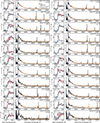 |
Fig. F.2. Same as Fig. F.1 |
| In the text | |
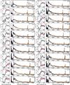 |
Fig. F.3. Same as Fig. F.1 |
| In the text | |
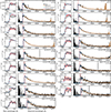 |
Fig. F.4. Same as Fig. F.1 |
| In the text | |
Current usage metrics show cumulative count of Article Views (full-text article views including HTML views, PDF and ePub downloads, according to the available data) and Abstracts Views on Vision4Press platform.
Data correspond to usage on the plateform after 2015. The current usage metrics is available 48-96 hours after online publication and is updated daily on week days.
Initial download of the metrics may take a while.