| Issue |
A&A
Volume 705, January 2026
|
|
|---|---|---|
| Article Number | A47 | |
| Number of page(s) | 10 | |
| Section | Interstellar and circumstellar matter | |
| DOI | https://doi.org/10.1051/0004-6361/202557107 | |
| Published online | 07 January 2026 | |
Radio-continuum spectra of pulsars with free-free thermal absorption
1
CONICET-Universidad Nacional de Córdoba, Instituto de Astronomía Teórica y Experimental (IATE),
Laprida 854,
X5000BGR,
Córdoba,
Argentina
2
Observatorio Astronómico, Universidad Nacional de Córdoba,
Laprida 854,
X5000BGR,
Córdoba,
Argentina
3
Instituto de Astronomía y Física del Espacio (IAFE), Ciudad Universitaria - Pabellón 2, Intendente Güiraldes
2160 (C1428EGA),
Ciudad Autónoma de Buenos Aires,
Argentina
4
Remote Sensing Division, Naval Research Laboratory,
Code 7213, 4555 Overlook Ave SW,
Washington, DC,
20375,
USA
★ Corresponding author: This email address is being protected from spambots. You need JavaScript enabled to view it.
Received:
4
September
2025
Accepted:
15
November
2025
Abstract
The radio continuum spectra of pulsars (PSRs) exhibit a wide variety of shapes, which are interpreted as pure and broken power laws, power laws with turnovers or cutoffs, and logarithmic-parabolic profiles. A notable fraction of these have well-defined power laws with ν−2.1 exponential turnovers, indicative of free-free thermal absorption along the line of sight. We analysed a sample of 63 PSRs with such spectral shapes, compiled from four previously published studies, to investigate their statistical properties. We normalised each spectrum to a characteristic frequency and flux density of its own, facilitating a consistent treatment across the four subsamples. We show that these two fitted parameters are correlated by a power law, with its slope reflecting the median spectral index (∼−2.0) of PSR emission. We find that the turnover frequencies in our sample are typically high, clustering around 558 MHz, which implies notably high emission measures (∼105 pc cm−6) for an inferred thermal absorbing medium with an electron temperature of 8000 K. Moreover, by combining these emission measures with dispersion measures derived from pulse time delays, we break the degeneracy between the electron density and the path length of the absorbers. This reveals a discrete near-in population of absorbers characterised by small sizes (∼0.1 pc) and high electron densities (∼103 cm−3), which exhibit a clear size-density anti-correlation reminiscent of that observed in Galactic and extragalactic H ii regions.
Key words: pulsars: general / ISM: clouds / ISM: general / ISM: structure
© The Authors 2026
 Open Access article, published by EDP Sciences, under the terms of the Creative Commons Attribution License (https://creativecommons.org/licenses/by/4.0), which permits unrestricted use, distribution, and reproduction in any medium, provided the original work is properly cited.
This article is published in open access under the Subscribe to Open model. This email address is being protected from spambots. You need JavaScript enabled to view it. to support open access publication.
1 Introduction
The study of pulsar (PSR) radio continuum spectra began in the 1970s, shortly after their discovery. Early works compiled flux density measurements across a range of frequencies, laying the groundwork for the first characterisations of their spectral behaviour. A seminal contribution came from Sieber (1973), who analysed spectra of PSRs using the observational data then available. Although each source was typically sampled at only a few frequencies, the study revealed that many PSR spectra follow a power-law trend, hinting at a relatively simple underlying emission mechanism. Sieber (1973) also noted in several cases that the spectra showed low-frequency turnovers, which he attributed to either synchrotron self-absorption (SSA) or thermal free-free absorption (FFA). These early findings highlighted the diversity of PSR spectral behaviour.
As observational capabilities expanded – in terms of both frequency coverage and sensitivity – it became increasingly evident that deviations from a simple power-law model are more common than initially thought. Nowadays, a variety of spectral features are observed, such as broken power laws, flattening, and turnovers, and they span a broad frequency range from ∼30 MHz up to ∼1 GHz (e.g. Swainston et al. 2022; Lee et al. 2022). These advances have been driven by dedicated PSR surveys accomplished with new-generation radio facilities, ranging from early initiatives such as the Parkes Southern Pulsar Survey (Manchester et al. 1996) to more recent ones such as the GMRT High Resolution Southern Sky Survey for Pulsars and Transients (GHRSS; Bhattacharyya et al. 2016), the LOFAR Tied-Array All-Sky Survey (LOTAAS; Sanidas et al. 2019), the Southern-sky MWA Rapid Two-metre pulsar survey (SMART; Bhat et al. 2023), the Green Bank 820 MHz Pulsar Survey (McEwen et al. 2024), the FAST Galactic Plane Snapshot Survey (GPPS; Han et al. 2025), and the NenuFAR Pulsar Blind Survey (NPBS; Brionne et al. 2025), among others. Despite this growing body of data, the physical origin of the observed spectral deviations – i.e. whether they stem from intrinsic properties of the PSR emission mechanism or arise from extrinsic propagation effects through intervening media – remains a matter of debate (e.g. Jankowski et al. 2018).
Of the various spectral features, exponential low-frequency attenuation consistent with FFA is increasing believed to be a tracer of ionised gas along the line of sight. Although FFA had already been proposed by Sieber (1973) to account for megahertz turnovers, more recent studies (e.g. Kijak et al. 2011; Lewandowski et al. 2015; Rajwade et al. 2016; Kijak et al. 2017; Basu et al. 2018; Kijak et al. 2021) have extended this interpretation to include higher-frequency turnovers, even reaching the gigahertz regime. These absorption signatures are thought to originate in diverse environments, such as filaments in supernova remnants (SNRs), bow shocks from PSR wind nebulae, H ii regions, or dense stellar winds in binary systems. In this context, modelling PSR spectra with exponential absorption functions provides a potentially powerful tool for probing the physical properties of the intervening ionised medium. In particular, the turnover frequency is sensitive to a combination of the electron density, path length, and electron temperature via the emission measure (EM). However, different combinations of these parameters can result in similar turnover frequencies, making it difficult to uniquely constrain the physical conditions of the absorber. One promising strategy for mitigating this degeneracy involves complementing spectral fits with independent constraints from dispersion measure (DM)-induced pulse time delays, which trace the total column density of free electrons along the line of sight (e.g. Rajwade et al. 2016; Kijak et al. 2021; Rożko et al. 2021). An additional complication arises from the use of different mathematical forms and conventions in the fitting equation of the spectra across the literature, which hinders direct comparisons between studies. Adopting a unique fitting equation facilitates comparisons across multiple samples, ultimately leading to insightful interpretations of the structures responsible for PSR absorption features.
This paper presents an analysis of PSR radio continuum spectra previously interpreted as bearing signatures of FFA. In Sect. 2 we employ the spectral modelling approach developed by Abadi et al. (2024) – which was originally designed to homogenise SNR spectra affected by thermal absorption – to our sample of PSRs with turnovers extending up to gigahertz frequencies. In Sect. 3 we examine correlations and differences in the fitted spectral parameters for PSRs and SNRs. The implications for the physical nature of the absorbing environments are discussed in Sect. 4. Finally, Sect. 5 provides a summary of our results.
2 Parameterisation and similarity in radio-continuum PSR spectra
The database used in our study comprises radio continuum spectra of 63 Galactic PSRs that span a broad frequency range from 20 MHz to 10 GHz. Among them, 15 were taken from Kijak et al. (2017, hereafter K17), 25 from Jankowski et al. (2018, J18), 10 from Kijak et al. (2021, K21), and 13 from Swainston et al. (2022, S22)1. These spectra are systematically modelled by a power law related to the PSR’s intrinsic radio emission with an exponential term that accounts for thermal FFA along the light of sight:
![Mathematical equation: $S(v) = {S_0}{\left( {{v \over {{v_0}}}} \right)^\alpha }\exp \left[ { - {\tau _0}{{\left( {{v \over {{v_0}}}} \right)}^{ - 2.1}}} \right].$](/articles/aa/full_html/2026/01/aa57107-25/aa57107-25-eq1.png) (1)
(1)
Here, S0 is a reference flux-density corresponding to an arbitrarily chosen reference frequency ν0, α is the power-law spectral index, and τ0 is the optical depth at ν0. The optical depth τ0 at frequency ν0, can be expressed as
 (2)
where Te is the mean electron temperature of the absorbing medium, a(ν0, Te) is the Gaunt factor correction – typically assumed to be of order unity (Wilson et al. 2009) – and the EM is defined as
(2)
where Te is the mean electron temperature of the absorbing medium, a(ν0, Te) is the Gaunt factor correction – typically assumed to be of order unity (Wilson et al. 2009) – and the EM is defined as
 (3)
with ne the free electron density and L the path length through the absorbing medium.
(3)
with ne the free electron density and L the path length through the absorbing medium.
Different authors have adopted slightly varied forms for Eq. (1), either adjusting the reference frequency or organising parameters differently. However, for PSR spectra affected by thermal FFA in the intervening medium, Eq. (1) consistently remains a three-parameter (S0, α, τ0) model for fitting measured flux densities, whereas the reference frequency ν0 is arbitrarily fixed by each author. Even though transitioning between parameter values in different expressions is straightforward, discrepancies in parameterisation complicate comparisons. Following Abadi et al. (2024), we applied their parameterisation for SNR continuum spectra to PSRs, i.e. we rewrote Eq. (1) in terms of a characteristic frequency, ν∗, and flux density, S∗:
![Mathematical equation: $S(v) = {S_*}{\left( {{v \over {{v_*}}}} \right)^\alpha }\exp \left[ { - {{\left( {{v \over {{v_*}}}} \right)}^{ - 2.1}}} \right].$](/articles/aa/full_html/2026/01/aa57107-25/aa57107-25-eq4.png) (4)
(4)
The characteristic frequency, ν*, is related to the radio spectral index (α) and the turnover frequency (νto, i.e. the frequency at which S (ν) reaches its maximum value from the fitting process) through the expression νto/ν* = (−2.1/α)1/2.1, while S* represents the spectral normalisation. This alternative formulation offers the key advantage of being independent of any reference frequency ν0. Indeed, by comparing Eqs. (1) and (4), it follows that  and S∗ = S0(ν*/ν0)α, implying that the characteristic parameters ν∗ and S∗ remain invariant under changes of reference frequency. Using these expressions along with the fitting parameters reported by K17, J18, K21, and S22, we derived the values of S* and ν* listed in Table A.1. Given the relationship between the characteristic frequency and the free-free optical depth, Eq. (2) can be rewritten as
 (5)
(5)
This expression shows that, assuming a fixed electron temperature, our fitting parameter ν∗ provides a direct estimate of the EM (see Sect. 4).
The panels in Fig. 1 separately display the radio continuum spectra of each PSR subsample (K17, J18, K21, and S22) considered in our analysis. To ensure that only spectra with robust fits were included, we selected those for which the chi-square statistic, χ2 = Σ (logSobs − logSfit)2/N, is lower than ~0.06, where Sobs and Sfit are the observed and modelled flux densities, respectively, and N is the number of data points used in the fit. Importantly, rather than performing new fits to the compiled data, we adopted the fitting parameters already published by the authors of each subsample to derive S* and ν* for Eq. (4). This selection based on χ2 led to the exclusion of 21 poorly fitted spectra from S22, while all spectra from K17 and K21 were retained. The J18 subsample, however, could not be subjected to this selection, as the individual flux density measurements were not published. In addition, as J18 provide only the turnover frequency and the spectral index, but not the fitted flux density scaling parameter (which sets the vertical normalisation of the spectrum), we recalculated the missing parameter using the spectral measurements compiled in the S22 repository. As both J18 and S22 compiled flux densities from the literature, we do not expect this procedure to introduce any systematic bias in the J18 spectra. Also, it is acknowledged that, in the case of a few PSRs for which only a single measurement causes the spectrum to deviate noticeably from a power law, these sources were tentatively included based on the available data. However, a definitive confirmation that their spectra indeed exhibit the characteristic signatures of FFA would require further investigation, which lies beyond the scope of this paper.
In Fig. 2 we illustrate our methodology by plotting the normalised flux density Sn(x) = S(ν)/S* = xα exp(−x−2.1) as a function of the normalised frequency x = ν/ν* for all the spectra depicted in Fig. 1. This new approach reveals a striking similarity in how PSR spectra exhibit turnovers at frequencies ν < ν∗, despite emitting with varying radio spectral indices. This behaviour is further illustrated in Fig. 3, where all PSR radio spectra are fitted using a unified absorption function A(x) = exp(−x−2.1), shown as the solid black curve. In Abadi et al. (2024), we demonstrated that SNR spectra often, but not uniformly, exhibit a drop-off at frequencies below 100 MHz due to thermal FFA. Here, we emphasise that a similar feature also characterises the spectral turnovers of PSRs, occurring at around 558 MHz. We highlight this property in Fig. 4, where we plot the ratio between the normalised flux densities and the power-law emission component of each PSR spectrum (blue symbols) as a function of the normalised frequency. For comparison, we include the 12 SNR spectra from Abadi et al. (2024, red symbols). While PSRs and SNRs follow the same exponential decay function, A(x), the scatter around the curve is noticeably larger for the 63 PSRs than for the SNRs. This discrepancy can be attributed to the more stringent selection criteria adopted by Castelletti et al. (2021) when constructing individual SNR spectra, rather than to any intrinsic difference in the spectral scatter between SNRs and PSRs. Moreover, the normalised flux measured at the lowest normalised frequency, x ~ 0.5, reaches a value of ∼0.01 for PSRs, compared to ∼0.1 for SNRs. This behaviour arises directly from the relation νto/ν* = (−2.1/α)1/2.1, which leads to ν∗ ~ νto for PSRs and ν∗ ≈ νto/2 for SNRs, given their different characteristic power-law indices, α ∼ −2.0 and −0.5, respectively.
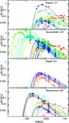 |
Fig. 1 Radio flux density measurements (coloured filled symbols) vs frequency for the four PSR subsamples analysed in our study. The panels, from top to bottom, display 15 spectra from K17, 25 from J18, 10 from K21, and 13 from S22. The solid coloured lines represent the best-fit models derived from Eq. (4) using spectral indices reported in the literature referenced in our work (see Table A.1 for the parameter values). Asterisks mark the characteristic frequency, ν∗, for each individual spectrum. |
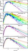 |
Fig. 2 Normalised radio flux density as a function of normalised frequency for our PSR sample, comprising (from top to bottom) 15 objects reported in K17, 25 in J18, 10 in K21, and 13 in S22. Each PSR within the subsamples is colour-coded individually. The solid lines represent the fitted models, with parameters listed in Table A.1, and the black asterisk indicates the characteristic frequency, ν*. This normalisation process highlights the similar exponential drop-off in the spectra associated with ν∗ values, arranging PSR spectra in increasing order based on the slope of their emission. |
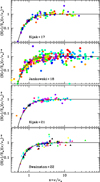 |
Fig. 3 Radio flux density, normalised by the characteristic flux and power-law emission, plotted against normalised frequency for the four subsamples in our study (see labels). Each spectrum was fitted by the respective authors with an exponential drop-off with an exponent −2.1. The curved solid line represents the normalised absorption function A(x) = exp(−x−2.1), and the asterisk indicates the characteristic frequency, ν∗. |
3 Spectral parameters correlations
The proposed parameterisation of PSR spectra in terms of S* and ν∗ (Eq. (4)) enables a homogeneous treatment of the four subsamples (K17, J18, K21, and S22), allowing us to analyse collectively the 63 spectra included in our compiled sample. This unified approach provides a consistent framework to investigate the statistical properties of the full dataset and to explore potential correlations among the fitted quantities. In Fig. 5 we display the mutual relation between S∗ and ν∗ for the PSRs (blue symbols). For comparison, we also include (red symbols) the corresponding values for a set of 12 SNR radio spectra with low-frequency turnovers presented in Abadi et al. (2024). The top panel shows histograms of the ν* distributions for both samples. The PSRs exhibit a median  MHz, which corresponds to a median
  MHz. In contrast, the SNRs show a significantly lower median
  MHz, equivalent to a turnover frequency of
  MHz. The slope of the observed correlation between ν∗ and S* primarily reflects the median of the distribution of spectral indices. In particular, for our PSR sample α values range from approximately 4.0 ≲ α ≲ −0.5 (see the blue histogram in the top panel of Fig. 6) with a median of
  in good agreement with the slope α = −1.94 obtained from the best-fit models applied to the data points. A similar trend is observed for the SNR sample, where the spectral indices span the range −1.0 ≲ α ≲ −0.3 (see the red histogram in the top panel of Fig. 6), with a median value of
  , closely matching the best-fit power-law slope α = −0.52. The S* values indicate the projected power-law flux density at ν∗ in the absence of absorption, while the short line segments indicate its slope. A visual inspection shows that, qualitatively, the slopes of these segments follow approximately the correlation exhibited by the data points themselves.
We also explored possible correlations between the spectral index α and both v* and S*, but found no significant trends, as shown in Figs. 6 and 7, respectively. The intrinsic emission from the source is described by the power-law function term in Eq. (4). Consequently, the luminosity can be readily estimated as  , where d represents the heliocentric distance to the source. We then extended our search for correlations between α and
 . One additional advantage of the parameterised spectral model (Eq. (4)) is the ability to integrate flux density over fixed values of normalised frequency x = v/v*, without the need to define vmin and vmax separately for each source. We used this feature to obtain an expression for the radio luminosity:
 (6)
(6)
Notice that in Eq. (6), no correction factor is included for the PSR emission beam solid angle or pulse duty cycle, as these are typically challenging to determine (Lorimer & Kramer 2004). Moreover, it is a common practice to define a pseudo-luminosity at a specified frequency, usually ν = 1400 MHz, as  , without explicitly integrating the power law between the minimum and maximum frequencies involved. The relationship between luminosity and spectral index is shown in Fig. 8, with a solid blue curve for PSRs and a solid red curve for SNRs. We adopted xmin = 0.01 and xmax = 1000, following the frequency coverage seen in Fig. 2. These curves are scaled using the median values for the parameters S*, ν*, and d for PSRs and SNRs (0.024 Jy, 500 MHz, and 4.06 kpc) and (140 Jy, 36 MHz, and 7 kpc), respectively. Since independent heliocentric distance measurements, such as those based on parallax, associations with other objects, or neutral hydrogen absorption measurements (especially for low-latitude PSRs), are not available for all PSRs in our collection, we used the distances reported in the Australia Telescope National Facility (ATNF) Pulsar Catalogue (Manchester et al. 2005)2, computed from DM estimates assuming the NE2001 model for the Galactic distribution of free electrons (Cordes & Lazio 2002, 2003). As can be seen in the blue and red curve, this analytically predicted luminosity decreases systematically with the spectral index until it reaches a critical value α0, which can be computed numerically by solving
 (7)
(7)
For the adopted xmin and xmax values, we obtain α0 ∼ −1.1. Expanding the integration interval has a minimal impact (e.g. increasing the range from xmin = 10−3 to xmax = 103 results in α0 ∼ −1). The asymptotic logarithmic slopes for spectral indices steeper and flatter than α0 are  and
and  , respectively. Using Eq. (6), we estimated the luminosity for each PSR in our sample and for the collection of SNRs with spectral turnovers. The wide range of spectral indices suggests a possible trend where luminosity data points decrease and then increase with the spectral indices, following the analytical curve. However, the limited number of PSRs with flatter spectral indices than α0 precludes a definitive confirmation of this trend.
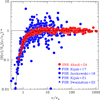 |
Fig. 4 Same PSR data as plotted in Fig. 3 but with the four subsamples merged (blue symbols). Additionally, data points for the SNRs presented in Abadi et al. (2024) are reproduced (red symbols). The graph highlights the similarity not only between the PSR spectra but also between the PSR and SNR spectral behaviours. The curved solid line is the normalised absorption, A(x) = exp(−x−2.1). |
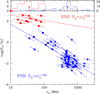 |
Fig. 5 Relation between the characteristic flux, S∗, and frequency, ν*, parameters obtained from fitting the parameterised free-free thermal absorption model (Eq. (4)) for our sample of 63 PSRs. For comparison, parameters calculated from the same model fit applied to 12 SNRs (Abadi et al. 2024) are also included. All data points are shown with the same symbols and colours as in Fig. 4. The long solid lines represent the best-fit linear relations for the PSR (blue) and SNR (red) parameters, with logarithmic slopes of −1.94 and −0.52, respectively. Short lines on each data point indicate the radio spectral index for each object, taken from K17, J18, K21, and S22 for PSRs and from Abadi et al. (2024) for SNRs. The median values of these spectral indices are consistent with the slopes of the power-law correlation between S* and ν*. The distribution of ν∗ values for PSRs and SNRs, with median values indicated by arrows, is shown in the blue and red histograms in the top panel. |
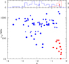 |
Fig. 6 Characteristic frequency, ν∗, fitted parameter in the model with an exponential drop-off of index −2.1 from Eq. (4) vs the spectral index of the radio emission for the PSRs in our sample, as reported in K17, J18, K21, and S22. Data points for PSRs are shown with blue symbols, as in Fig. 4, and data for SNR spectra with exponential turnovers from Abadi et al. (2024) are shown as red circles. No correlation between the plotted parameters is evident. The histograms in the top panel show the distribution of α values for the collection of PSRs (blue) and SNRs (red), with median values marked by arrows. |
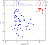 |
Fig. 7 Power-law slope, α, vs the characteristic flux density, S*, fitted parameter in Eq. (4) for our collection of 63 PSRs. The spectral index values are those reported in K17, J18, K21, and S22. Blue symbols are coded as in Fig. 4. Red symbols denote SNR data from exponential turnover fits as presented in Abadi et al. (2024). No correlation between the plotted parameters is evident. The histograms in the top panel illustrate the distribution of S∗ values for PSRs (blue) and SNRs (red), with median values marked by arrows. |
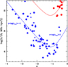 |
Fig. 8 Integrated luminosity plotted against the power-law spectral index, α, for our sample of PSRs (blue symbols, as in Fig. 4) and SNRs (red symbols, from Abadi et al. 2024). The luminosity is computed by integrating the power-law flux density emission between normalised frequencies xmin = 10−2 and xmax = 103. Notice that changing the frequency range over which the integration is performed modifies the asymptotic logarithmic slopes, γ, at the low and high ends of α, corresponding to log(xmin) and log(xmax), respectively. The solid blue and red curves are derived using Eq. (8), with pre-factor parameters S*, ν*, and d given by the corresponding median values for PSRs and SNRs. |
4 Physical conditions in the thermal free-free absorbers
Building on the results presented in the previous sections, we now focus on the physical conditions of the ionised medium responsible for the thermal FFA observed in the PSR radio spectra. As a starting point, we constructed a face-on view of the Galactic plane showing the spatial distribution of the PSRs in our sample (Fig. 9), using distances inferred from the NE2001 model. This representation enables us to infer the likely locations of the absorbers responsible for the observed spectral turnovers, based on the positions of the PSRs, and provides insight into their distribution relative to large-scale Galactic structures. Although the PSRs in our sample are primarily distributed within the first and fourth Galactic quadrants and extend up to ∼8 kpc – thus reaching the vicinity of the Galactic centre – this spatial coverage is sufficient to derive representative physical properties of the absorbing media.
To further constrain the properties of the ionised medium, we combined the DMs reported in the ATNF Pulsar Catalogue (Manchester et al. 2005) with the EMs derived from our spectral fits, using the relation given in Eq. (5). For this calculation, we adopted a representative electron temperature of Te = 8000 K, consistent with typical values in H ii regions and other diffuse ionised environments (e.g. Quireza et al. 2006; Luisi et al. 2019). Figure 10 presents the resulting EM–DM diagram, where each filled symbol corresponds to a PSR in our sample. The location of the data points in Fig. 10 confirms that the observed spectral turnovers correspond to exceptionally high EMs. Given that our sample has a relatively high median turnover frequency (ν∗ ≈ 500 MHz, that is, νto ≈ 558 MHz), the resulting EMs are correspondingly large, reaching values up to ∼105 pc cm−6. These values are consistent with those reported by Rajwade et al. (2016) for a sample of six PSRs with GHz spectral turnovers (see their Table 1).
To further highlight the extremely high values inferred from such high-frequency turnovers, we also show the NE2001 model estimates for each PSR in our sample (open symbols in Fig. 10). The NE2001 model assumes a smoothly distributed ionised medium along the line of sight and estimates the EM (Eq. (3)) based on its internal electron density distribution. In addition, Fig. 10 displays the broader EM versus DM distribution predicted by NE2001 for the ATNF PSR population (shown as blue dots). Notably, the PSRs in our sample appear to constitute a representative subsample of this general population, showing no evident bias towards particular values of either the EM or DM, as indicated by the overlap between the open symbols and the cloud of blue dots. In contrast to the relatively tight EM–DM correlation expected from a smooth medium, the EMs values derived from our spectral fits show no clear trend with DMs. This discrepancy suggests that the absorbing material traced by the spectral turnovers is likely dominated by compact and possibly clumpy structures, rather than by a uniformly distributed ionised component. In this sense, our results reinforce the interpretation of thermal absorption as a localised phenomenon shaped by environmental inhomogeneities along the line of sight.
Combining EMs values derived from spectral analysis with DMs obtained from timing observations allows us to disentangle the degeneracy between electron density and absorber size. EM and DM can be expressed as  and
and  , assuming a constant electron density along the path length (L). From these relations, we can estimate the electron density ne = EM/DM and the physical size L = DM2/EM of the absorbing region. Then, under this simplified model, lines of constant absorber size L in the EM-DM diagram follow a power law with logarithmic slope 2, with the intercept increasing with L, as illustrated by the dotted lines in Fig. 10. Applying these expressions to our sample yields small absorber sizes, most of them typically in the range 0.01 to 1 pc, balanced by high electron densities of a few times 103 cm−3. In contrast, the EMs values derived using the NE2001 model correspond to much lower electron densities (~10−1 cm−3) integrated throughout much larger sizes corresponding to the PSR distance. Notably, high-density, compact absorbers have been previously proposed by several authors as the cause of GHz-frequency spectral turnovers in PSRs. For example, Lewandowski et al. (2015), Rajwade et al. (2016), Kijak et al. (2017), and Kijak et al. (2021) all suggest that such dense, localised structures – such as SNR filaments, bow shocks, or compact H ii regions – can imprint exponential absorption signatures on the radio spectra of PSRs.
Further analysis presented in Fig. 11 shows the correlation between ne and L, revealing a simple scaling law in which the electron density decreases as the size of the absorbers increases. The characteristic densities of approximately 5 × 103 cm−3, combined with sizes around 5 × 10⁻² pc, indicate that the absorbers are both compact and extremely dense. The best-fit regression solution for our data points corresponds to  , with a highly significant correlation coefficient r = −0.86. Notably, similar power-law relationships between the sizes and electron densities of ionised regions (ne ∝ D−1, where D is the diameter of the ionised regions; Hunt & Hirashita 2009, and references therein) have been found in studies of Galactic and extragalactic H ii region populations. In Fig. 11 we compare the scaling observed in our PSR sample with the trend reported in H ii regions, reproducing the data points used by Hunt & Hirashita (2009) in Fig. 2 of their work. Therefore, our result indicates that the radio continuum radiation from PSRs is absorbed by individual clumps, which follow an electron density-size relationship akin to that of the H ii regions. We notice that both the electron density squared and the absorber size scale with
  (see Eq. (5)). This implies that relaxing the assumption of Te = 8000 K to a lower (or higher) temperature would result in a corresponding decrease (or increase) in the absorber’s electron density, while the absorber size would conversely increase (or decrease). Despite these variations in temperature assumptions, the observed correlation remains consistent across different scenarios.
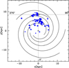 |
Fig. 9 Projected spatial distribution of our sample of 63 PSRs onto the Galactic plane. Distance estimates for the PSRs were taken from the ATNF catalogue (Manchester et al. 2005) and are based on the NE2001 Galactic electron-density model (Cordes & Lazio 2002, 2003). Pentagons correspond to K17 data, circles to J18, squares to K21, and triangles to S22. For guidance, the solid black lines show the positions of the spiral arms according to the Hou & Han (2014) model. The central plus symbol marks the position of the Galactic centre, the solar symbol shows the Sun’s position, and dotted lines outline the Galactic quadrants. |
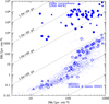 |
Fig. 10 EMs plotted against DMs for the 63 PSRs included in our sample. Filled symbols correspond to EMs values derived from radio continuum spectral turnovers in K17 (pentagons), J18 (circles), K21 (squares), and S22 (triangles). Open blue symbols represent EMs values predicted by the NE2001 model (Cordes & Lazio 2002, 2003) for our collection of PSRs, while the smallest blue points indicate values derived for all PSRs in the ATNF catalogue. The diagonal dotted lines show the relationship for constant size values, as labelled. |
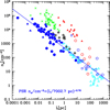 |
Fig. 11 Relation between the electron number density, ne, and the size, L, of the absorber population causing turnovers at ν* < 2 GHz in our sample of 63 PSR radio continuum spectra, modelled by a power law with a turnover due to free-free thermal absorption. Filled blue symbols represent data from PSR spectra in K17 (pentagons), J18 (circles), K21 (squares), and S22 (triangles). The solid blue line represents the least-squares fit to the PSR data, ne ∝ L−0.70, assuming an electron temperature of the ionised gas Te = 8000 K. The graphic also reproduces the data points from Fig. 2 of Hunt & Hirashita (2009), corresponding to Galactic ultracompact (cyan plus symbols), compact (green crosses), and giant (open cyan triangles) H ii regions, along with different extragalactic H ii region samples: radio galaxies (filled red triangles), Small and Large Magellanic Clouds (black open stars), M33 (open blue squares), Zw18 (filled blue triangles), dwarf galaxies observed with HST (open red and blue circles), and spiral and irregular galaxies (open cyan triangles). The correlation we find between the size and density of the PSR radio emission absorbers is consistent with that observed in Galactic and extragalactic H ii regions (ne ∝ L−1). |
5 Summary
We have statistically analysed a sample of 63 PSR radio continuum spectra drawn from the literature, each modelled with a power law and an exponential turnover attributed to thermal FFA in the intervening ionised gas between the PSR and the observer. Our key findings are summarised as follows:
We introduced a parameterisation of PSR radio continuum spectra in terms of a characteristic frequency, ν∗, and its corresponding flux density, S∗, which enables the homogenisation of different subsamples drawn from previously published studies. This approach eliminates the reliance on an arbitrarily chosen reference frequency, allowing for consistent comparisons across heterogeneous datasets.
By utilising ν∗ and S∗ and normalising each spectrum to its intrinsic power-law emission, we show that the stacked flux density measurements accurately trace the drop-off caused by thermal absorption, reaching flux density levels that are approximately two orders of magnitude below the flux density at the spectral turnover.
Parameterising the PSR spectra revealed a correlation between the characteristic flux density and frequency, with a slope that reflects the median radio spectral index (∼ −2.0) of the PSR sample. We also reinforced this behaviour in the case of SNRs, which exhibit significantly flatter spectra (∼ −0.5).
By combining the EMs inferred from PSR radio spectral turnovers with independently determined DMs from pulse time delays, we estimated characteristic electron densities and path lengths for the putative population of absorbers. The resulting values point to a population of clumpy, near-in absorbers, with compact sizes (L) of the order of ~0.1 pc and relatively high electron densities (ne) of ∼103 cm−3, as measured towards SNRs.
The absorbing structures follow a size-density anti-correlation of the form ne ∝ L−0.70, reminiscent of the well-established empirical relation observed in Galactic and extragalactic H ii regions.
Acknowledgements
We thank a very constructive and insightful report from an anonymous referee that improved the previous version of the paper. We also thank Dale Frail and Stella Ocker for a careful reading and comments on a previous version of the paper. This work has been partially supported by the Consejo de Investigaciones Científicas y Técnicas de la República Argentina (CONICET, PIP 11220220100337), the Secretaría de Ciencia y Técnica de la Universidad Nacional de Córdoba (SeCyT), Agencia Nacional de Promoción Científica y Tecnológica (PICT 2019-1600), Argentina. Basic research in radio astronomy at the Naval Research Laboratory is funded by 6.1 Base funding.
References
- Abadi, M. G., Castelletti, G., Supan, L., Kassim, N. E., & Lazio, J. W. 2024, A&A, 684, A54 [NASA ADS] [CrossRef] [EDP Sciences] [Google Scholar]
- Basu, R., RoŻko, K., Kijak, J., & Lewandowski, W. 2018, MNRAS, 475, 1469 [Google Scholar]
- Bhat, N. D. R., Swainston, N. A., McSweeney, S. J., et al. 2023, PASA, 40, e020 [Google Scholar]
- Bhattacharyya, B., Cooper, S., Malenta, M., et al. 2016, ApJ, 817, 130 [NASA ADS] [CrossRef] [Google Scholar]
- Brionne, M., Grießmeier, J. M., Cognard, I., et al. 2025, A&A, 693, A96 [NASA ADS] [CrossRef] [EDP Sciences] [Google Scholar]
- Castelletti, G., Supan, L., Peters, W. M., & Kassim, N. E. 2021, A&A, 653, A62 [NASA ADS] [CrossRef] [EDP Sciences] [Google Scholar]
- Cordes, J. M., & Lazio, T. J. W. 2002, arXiv e-prints [arXiv:astro-ph/0207156] [Google Scholar]
- Cordes, J. M., & Lazio, T. J. W. 2003, arXiv e-prints [arXiv:astroph/0301598] [Google Scholar]
- Han, J. L., Zhou, D. J., Wang, C., et al. 2025, Res. Astron. Astrophys., 25, 014001 [Google Scholar]
- Hou, L. G., & Han, J. L. 2014, A&A, 569, A125 [NASA ADS] [CrossRef] [EDP Sciences] [Google Scholar]
- Hunt, L. K., & Hirashita, H. 2009, A&A, 507, 1327 [NASA ADS] [CrossRef] [EDP Sciences] [Google Scholar]
- Jankowski, F., van Straten, W., Keane, E. F., et al. 2018, MNRAS, 473, 4436 [Google Scholar]
- Kijak, J., Dembska, M., Lewandowski, W., Melikidze, G., & Sendyk, M. 2011, MNRAS, 418, L114 [Google Scholar]
- Kijak, J., Basu, R., Lewandowski, W., Rożko, K., & Dembska, M. 2017, ApJ, 840, 108 [Google Scholar]
- Kijak, J., Basu, R., Lewandowski, W., & Rożko, K. 2021, ApJ, 923, 211 [Google Scholar]
- Lee, C. P., Bhat, N. D. R., Sokolowski, M., et al. 2022, PASA, 39, e042 [Google Scholar]
- Lewandowski, W., Rożko, K., Kijak, J., & Melikidze, G. I. 2015, ApJ, 808, 18 [Google Scholar]
- Lorimer, D. R., & Kramer, M. 2004, Handbook of Pulsar Astronomy (Cambridge: Cambridge University Press), 4 [Google Scholar]
- Luisi, M., Anderson, L. D., Liu, B., Anish Roshi, D., & Churchwell, E. 2019, ApJS, 241, 2 [Google Scholar]
- Manchester, R. N., Lyne, A. G., D’Amico, N., et al. 1996, MNRAS, 279, 1235 [Google Scholar]
- Manchester, R. N., Hobbs, G. B., Teoh, A., & Hobbs, M. 2005, AJ, 129, 1993 [Google Scholar]
- McEwen, A. E., Lynch, R. S., Kaplan, D. L., et al. 2024, ApJ, 969, 118 [Google Scholar]
- Quireza, C., Rood, R. T., Bania, T. M., Balser, D. S., & Maciel, W. J. 2006, ApJ, 653, 1226 [Google Scholar]
- Rajwade, K., Lorimer, D. R., & Anderson, L. D. 2016, MNRAS, 455, 493 [Google Scholar]
- Rożko, K., Basu, R., Kijak, J., & Lewandowski, W. 2021, ApJ, 922, 125 [Google Scholar]
- Sanidas, S., Cooper, S., Bassa, C. G., et al. 2019, A&A, 626, A104 [NASA ADS] [CrossRef] [EDP Sciences] [Google Scholar]
- Sieber, W. 1973, A&A, 28, 237 [NASA ADS] [Google Scholar]
- Swainston, N. A., Lee, C. P., McSweeney, S. J., & Bhat, N. D. R. 2022, PASA, 39, e056 [Google Scholar]
- Wilson, T. L., Rohlfs, K., & Hüttemeister, S. 2009, Tools of Radio Astronomy (Berlin: Springer) [Google Scholar]
Swainston et al. (2022) refers to an open-source repository that centralises PSR flux density measurements. The data included in our paper correspond to the catalogue update available at the time of writing.
Web address http://www.atnf.csiro.au/research/pulsar/psrcat
Appendix A PSR radio-continuum spectral parameters
PSR radio-continuum spectral parameters.
All Tables
All Figures
|
Fig. 1 Radio flux density measurements (coloured filled symbols) vs frequency for the four PSR subsamples analysed in our study. The panels, from top to bottom, display 15 spectra from K17, 25 from J18, 10 from K21, and 13 from S22. The solid coloured lines represent the best-fit models derived from Eq. (4) using spectral indices reported in the literature referenced in our work (see Table A.1 for the parameter values). Asterisks mark the characteristic frequency, ν∗, for each individual spectrum. |
| In the text | |
|
Fig. 2 Normalised radio flux density as a function of normalised frequency for our PSR sample, comprising (from top to bottom) 15 objects reported in K17, 25 in J18, 10 in K21, and 13 in S22. Each PSR within the subsamples is colour-coded individually. The solid lines represent the fitted models, with parameters listed in Table A.1, and the black asterisk indicates the characteristic frequency, ν*. This normalisation process highlights the similar exponential drop-off in the spectra associated with ν∗ values, arranging PSR spectra in increasing order based on the slope of their emission. |
| In the text | |
|
Fig. 3 Radio flux density, normalised by the characteristic flux and power-law emission, plotted against normalised frequency for the four subsamples in our study (see labels). Each spectrum was fitted by the respective authors with an exponential drop-off with an exponent −2.1. The curved solid line represents the normalised absorption function A(x) = exp(−x−2.1), and the asterisk indicates the characteristic frequency, ν∗. |
| In the text | |
|
Fig. 4 Same PSR data as plotted in Fig. 3 but with the four subsamples merged (blue symbols). Additionally, data points for the SNRs presented in Abadi et al. (2024) are reproduced (red symbols). The graph highlights the similarity not only between the PSR spectra but also between the PSR and SNR spectral behaviours. The curved solid line is the normalised absorption, A(x) = exp(−x−2.1). |
| In the text | |
|
Fig. 5 Relation between the characteristic flux, S∗, and frequency, ν*, parameters obtained from fitting the parameterised free-free thermal absorption model (Eq. (4)) for our sample of 63 PSRs. For comparison, parameters calculated from the same model fit applied to 12 SNRs (Abadi et al. 2024) are also included. All data points are shown with the same symbols and colours as in Fig. 4. The long solid lines represent the best-fit linear relations for the PSR (blue) and SNR (red) parameters, with logarithmic slopes of −1.94 and −0.52, respectively. Short lines on each data point indicate the radio spectral index for each object, taken from K17, J18, K21, and S22 for PSRs and from Abadi et al. (2024) for SNRs. The median values of these spectral indices are consistent with the slopes of the power-law correlation between S* and ν*. The distribution of ν∗ values for PSRs and SNRs, with median values indicated by arrows, is shown in the blue and red histograms in the top panel. |
| In the text | |
|
Fig. 6 Characteristic frequency, ν∗, fitted parameter in the model with an exponential drop-off of index −2.1 from Eq. (4) vs the spectral index of the radio emission for the PSRs in our sample, as reported in K17, J18, K21, and S22. Data points for PSRs are shown with blue symbols, as in Fig. 4, and data for SNR spectra with exponential turnovers from Abadi et al. (2024) are shown as red circles. No correlation between the plotted parameters is evident. The histograms in the top panel show the distribution of α values for the collection of PSRs (blue) and SNRs (red), with median values marked by arrows. |
| In the text | |
|
Fig. 7 Power-law slope, α, vs the characteristic flux density, S*, fitted parameter in Eq. (4) for our collection of 63 PSRs. The spectral index values are those reported in K17, J18, K21, and S22. Blue symbols are coded as in Fig. 4. Red symbols denote SNR data from exponential turnover fits as presented in Abadi et al. (2024). No correlation between the plotted parameters is evident. The histograms in the top panel illustrate the distribution of S∗ values for PSRs (blue) and SNRs (red), with median values marked by arrows. |
| In the text | |
|
Fig. 8 Integrated luminosity plotted against the power-law spectral index, α, for our sample of PSRs (blue symbols, as in Fig. 4) and SNRs (red symbols, from Abadi et al. 2024). The luminosity is computed by integrating the power-law flux density emission between normalised frequencies xmin = 10−2 and xmax = 103. Notice that changing the frequency range over which the integration is performed modifies the asymptotic logarithmic slopes, γ, at the low and high ends of α, corresponding to log(xmin) and log(xmax), respectively. The solid blue and red curves are derived using Eq. (8), with pre-factor parameters S*, ν*, and d given by the corresponding median values for PSRs and SNRs. |
| In the text | |
|
Fig. 9 Projected spatial distribution of our sample of 63 PSRs onto the Galactic plane. Distance estimates for the PSRs were taken from the ATNF catalogue (Manchester et al. 2005) and are based on the NE2001 Galactic electron-density model (Cordes & Lazio 2002, 2003). Pentagons correspond to K17 data, circles to J18, squares to K21, and triangles to S22. For guidance, the solid black lines show the positions of the spiral arms according to the Hou & Han (2014) model. The central plus symbol marks the position of the Galactic centre, the solar symbol shows the Sun’s position, and dotted lines outline the Galactic quadrants. |
| In the text | |
|
Fig. 10 EMs plotted against DMs for the 63 PSRs included in our sample. Filled symbols correspond to EMs values derived from radio continuum spectral turnovers in K17 (pentagons), J18 (circles), K21 (squares), and S22 (triangles). Open blue symbols represent EMs values predicted by the NE2001 model (Cordes & Lazio 2002, 2003) for our collection of PSRs, while the smallest blue points indicate values derived for all PSRs in the ATNF catalogue. The diagonal dotted lines show the relationship for constant size values, as labelled. |
| In the text | |
|
Fig. 11 Relation between the electron number density, ne, and the size, L, of the absorber population causing turnovers at ν* < 2 GHz in our sample of 63 PSR radio continuum spectra, modelled by a power law with a turnover due to free-free thermal absorption. Filled blue symbols represent data from PSR spectra in K17 (pentagons), J18 (circles), K21 (squares), and S22 (triangles). The solid blue line represents the least-squares fit to the PSR data, ne ∝ L−0.70, assuming an electron temperature of the ionised gas Te = 8000 K. The graphic also reproduces the data points from Fig. 2 of Hunt & Hirashita (2009), corresponding to Galactic ultracompact (cyan plus symbols), compact (green crosses), and giant (open cyan triangles) H ii regions, along with different extragalactic H ii region samples: radio galaxies (filled red triangles), Small and Large Magellanic Clouds (black open stars), M33 (open blue squares), Zw18 (filled blue triangles), dwarf galaxies observed with HST (open red and blue circles), and spiral and irregular galaxies (open cyan triangles). The correlation we find between the size and density of the PSR radio emission absorbers is consistent with that observed in Galactic and extragalactic H ii regions (ne ∝ L−1). |
| In the text | |
Current usage metrics show cumulative count of Article Views (full-text article views including HTML views, PDF and ePub downloads, according to the available data) and Abstracts Views on Vision4Press platform.
Data correspond to usage on the plateform after 2015. The current usage metrics is available 48-96 hours after online publication and is updated daily on week days.
Initial download of the metrics may take a while.