| Issue |
A&A
Volume 706, February 2026
|
|
|---|---|---|
| Article Number | A136 | |
| Number of page(s) | 24 | |
| Section | Extragalactic astronomy | |
| DOI | https://doi.org/10.1051/0004-6361/202555981 | |
| Published online | 05 February 2026 | |
Clumpiness of galaxies revealed in the near-infrared with COSMOS-Web
Substructures at 1 < z < 4 and their link to stellar mass and star formation
1
Aix Marseille Univ, CNRS, CNES, LAM Marseille, France
2
Kavli Institute for Astronomy and Astrophysics, Peking University Beijing 100871, People’s Republic of China
3
Kavli IPMU (WPI), UTIAS, The University of Tokyo, Kashiwa Chiba 277-8583, Japan
4
Cosmic Dawn Center (DAWN), Denmark
5
Niels Bohr Institute, University of Copenhagen Jagtvej 128 2200 Copenhagen, Denmark
6
Institut d’Astrophsyique de Paris, UMR 7095, CNRS, UPMC Univ. Paris VI 98 bis boulevard Arago Paris, France
7
Department of Physics and Astronomy, University of California, Riverside 900 University Avenue Riverside CA 92521, USA
8
Laboratory for Multiwavelength Astrophysics, School of Physics and Astronomy, Rochester Institute of Technology 84 Lomb Memorial Drive Rochester NY 14623, USA
9
Caltech/IPAC, MS 314-6 1200 E. California Blvd. Pasadena CA 91125, USA
10
LUX, Observatoire de Paris, Université PSL, Sorbonne Université, CNRS 75014 Paris, France
11
Department of Astronomy, School of Science, The University of Tokyo 7-3-1 Hongo Bunkyo Tokyo 113-0033, Japan
12
Institute of Physics, GalSpec, Ecole Polytechnique Federale de Lausanne, Observatoire de Sauverny Chemin Pegasi 51 1290 Versoix, Switzerland
13
INAF, Astronomical Observatory of Trieste Via Tiepolo 11 34131 Trieste, Italy
14
Instituto de Astrofísica de Canarias C/ Vía Láctea s/n 38205 La Laguna Tenerife, Spain
15
Departamento de Astrofísica, Universidad de La Laguna 38200 La Laguna Tenerife, Spain
16
Observatoire de Paris, LERMA, PSL University 61 avenue de l’Observatoire F-75014 Paris, France
17
Université Paris-Cité 5 Rue Thomas Mann 75014 Paris, France
18
Department of Astronomy, The University of Washington Seattle WA 98195, USA
19
Space Telescope Science Institute 3700 San Martin Drive Baltimore MD 21218, USA
20
Department of Computer Science, Aalto University P.O. Box 15400 FI-00076 Espoo, Finland
21
Department of Physics, University of P.O. Box 64 FI-00014 Helsinki, Finland
22
Department of Physics and Astronomy, UCLA, PAB 430 Portola Plaza Box 951547 Los Angeles CA 90095-1547, USA
23
Jet Propulsion Laboratory, California Institute of Technology 4800 Oak Grove Drive Pasadena CA 91001, USA
24
Department of Physics, University of California, Santa Barbara Santa Barbara CA 93106, USA
25
The University of Texas at Austin 2515 Speedway Blvd Stop C1400 Austin TX 78712, USA
26
Department of Astronomy and Astrophysics, University of California, Santa Cruz 1156 High Street Santa Cruz CA 95064, USA
27
Université Paris-Saclay, Université Paris Cité, CEA, CNRS, AIM 91191 Gif-sur-Yvette, France
28
Purple Mountain Observatory, Chinese Academy of Sciences 10 Yuanhua Road Nanjing 210023, China
★ Corresponding author: This email address is being protected from spambots. You need JavaScript enabled to view it.
Received:
16
June
2025
Accepted:
14
November
2025
Abstract
Context. Clumps in the rest-frame UV emission of galaxies at z ≲ 3 have been observed for decades. Since the launch of the James Webb Space Telescope (JWST), a large population is detected in the rest-frame near-infrared (NIR), raising questions about their formation mechanism.
Aims. We investigate the presence and properties of NIR overdensities (hereafter substructures, including clumps) in star-forming and quiescent galaxies at 1 < z < 4 to understand their link to the evolution of their host galaxy.
Methods. We identified substructures in JWST/NIRCam F277W and F444W residual images at a rest-frame wavelength of 1 μm.
Results. The fraction of galaxies with substructures with M★ > 109 M⊙ has steadily decreased with cosmic time from 40% at z = 4 to 10% at z = 1. NIR clumps, the most common type of small substructure, are much fainter (2% of the total galaxy flux) than similar UV clumps in the literature. Nearly all galaxies at the high-mass end of the main sequence (MS), starburst, and green valley regions have substructures. However, we do not find substructures in low-mass galaxies in the green valley and red sequence. Although massive galaxies on the MS and in the green valley have a 40% probability of hosting multiple clumps, the majority of clumpy galaxies host only a single clump.
Conclusions. The fraction of clumpy galaxies in the rest-frame NIR is determined by the stellar mass and star formation rate (SFR) of the host galaxies. Its evolution with redshift is due to galaxies moving toward lower SFRs at z ≲ 2 and the buildup of low-mass galaxies in the green valley and red sequence. Based on their spatial distribution in edge-on galaxies, we infer that most substructures are produced in situ via disk fragmentation. Galaxy mergers may still play a role at high stellar masses, especially at a low SFR.
Key words: galaxies: evolution / galaxies: fundamental parameters / galaxies: general / galaxies: statistics / galaxies: stellar content / galaxies: structure
Kavli Astrophysics Fellow and Boya Fellow.
© The Authors 2026
 Open Access article, published by EDP Sciences, under the terms of the Creative Commons Attribution License (https://creativecommons.org/licenses/by/4.0), which permits unrestricted use, distribution, and reproduction in any medium, provided the original work is properly cited.
This article is published in open access under the Subscribe to Open model. This email address is being protected from spambots. You need JavaScript enabled to view it. to support open access publication.
1. Introduction
The morphology of galaxies is now known to have evolved tremendously with redshift in terms of size (e.g., Williams et al. 2010; van der Wel et al. 2014b; Martorano et al. 2024; Yang et al. 2025), stellar density (e.g., Williams et al. 2010), and overall 3D shape (e.g., van der Wel et al. 2014a; Huertas-Company et al. 2024). With the advent of the Hubble Space Telescope (HST), one striking feature in high-resolution images has been the presence of kiloparsec-scale, bright, local overdensities observed in the rest-frame ultraviolet (UV), referred to as clumps (e.g., Conselice et al. 2004; Elmegreen et al. 2005; Förster Schreiber et al. 2011a,b; Guo et al. 2015, 2018; Ribeiro et al. 2017). Importantly, these clumps have been found to be ubiquitous, with fractions of clumpy star-forming galaxies in the rest-frame UV reaching typical values of 25% at M★ ∼ 109.5 M⊙ and going up to 40% at 1011 M⊙, with little variation with redshift for 1 < z < 3 (e.g., Huertas-Company et al. 2020). In addition, they were originally estimated to be particularly massive (M★ ≳ 109 M⊙, e.g., Förster Schreiber et al. 2011b) without similarly massive counterparts known in the local Universe (M★ ≲ 107 M⊙ at z ∼ 0, e.g., Elmegreen & Salzer 1999). This naturally raised questions regarding their origin and fate, which have been investigated from the point of view of both observations and simulations. For instance, Genzel et al. (2011) found that UV clumps in star-forming galaxies at z ∼ 2 reside in regions where gravitational instabilities are likely to take place, thus favoring disk fragmentation as the mechanism behind their formation. This mechanism is also favored by Guo et al. (2015), Zanella et al. (2019), and Sattari et al. (2023). In particular, Zanella et al. (2019) show that compact UV clumps have, on average, lower stellar masses and ages than their host galaxies but comparable star formation rates (SFRs), suggesting in situ formation. However, Guo et al. (2015) show that minor mergers could be a more plausible scenario for galaxies with intermediate stellar masses at z < 1.5. Furthermore, for the brightest galaxies in the rest-frame UV, Ribeiro et al. (2017) consider instead a major merger origin by arguing that a significant proportion of bright galaxies host two clumps of a similar luminosity, which is insufficient compared to the number produced by disk fragmentation inside simulations (typically between five and ten, e.g., Perez et al. 2013; Bournaud et al. 2014). Indeed, simulations from Perez et al. (2013), Bournaud et al. (2014), Mayer et al. (2016), Tamburello et al. (2017), Fensch & Bournaud (2021), and Renaud et al. (2024) show that it is possible to form massive clumps via fragmentation in galaxies at 1 ≲ z ≲ 3 without invoking galaxy mergers. Theoretically, this scenario is supported by early analytical stability analyses that showed that fragmentation can occur in various types of media (Jeans 1902; Toomre 1964). Since then, these works have been extended by Romeo et al. (2010) and Romeo & Agertz (2014) who have shown that star-forming galaxies at a high redshift that host a thick and turbulent gas disk are prone to fragmentation under three main types of instabilities, including in marginally stable galaxies as evidenced by observations (e.g., Genzel et al. 2014). According to Perez et al. (2013) and Bournaud et al. (2014), clumps with masses around 109 M⊙ are sufficiently long-lived to migrate toward the galaxy center in less than 1 Gyr and may be a viable channel for bulge growth, funneling gas inward and migrating gas outward (e.g., Bournaud et al. 2011; Dubois et al. 2012; Xu & Yu 2024; Yu et al. 2025). However, smaller clumps may be disrupted by feedback processes (e.g., Bournaud et al. 2014; Mayer et al. 2016) or by strong local shear (Fensch & Bournaud 2021), thus leading to simulations where only small clumps can be formed and migration is not possible (e.g., in the FIRE simulation, Oklopčić et al. 2017). Observationally, this has been confirmed by Faisst et al. (2025) for starbursts at z < 4 where they find that the fraction of clumpy galaxies is correlated to the star formation efficiency and is higher in the starburst regime. High-resolution observations of clumps in lensed galaxies (e.g., see Fig. 9 of Claeyssens et al. 2023) also show that more massive clumps tend to be older (10 Myr at 105.5 M⊙ versus 1 Gyr at 107 M⊙) and more gravitationally bound. In addition, Fensch & Bournaud (2021) and Renaud et al. (2024) find that the clumpiness of galaxies is primarily determined by their gas content. In contrast, Perez et al. (2013) indicated that fragmentation is significantly more probable to happen in a multiphase interstellar medium with temperatures on the order of 104 K. This is, at the very least, mildly supported by observations (e.g., see Fig. 9 of Übler et al. 2019).
It is important to note that the existence, or at least the prevalence, of massive UV clumps remains a topic of debate due to the spatial resolution limitations of HST in the UV that prevents the resolution of clumps on scales smaller than approximately 1 kpc for galaxies at z > 1 (e.g., Dessauges-Zavadsky et al. 2017; Dessauges-Zavadsky & Adamo 2018; Huertas-Company et al. 2020). A similar debate is currently taking place for clumps detected with the James Webb Space Telescope (JWST) in the near infrared (NIR; e.g., Claeyssens et al. 2023, 2025). Thanks to the magnifying power of gravitational lensing, it is possible to resolve fainter and smaller clumps in lensed galaxies down to approximately 100 pc with HST (e.g., Adamo et al. 2013; Dessauges-Zavadsky et al. 2017; Dessauges-Zavadsky & Adamo 2018) and 10 pc with JWST (e.g., Claeyssens et al. 2023, 2025). The key takeaway from these analyses is that massive UV and optical clumps are nearly absent from lensed galaxies, with clump stellar masses around 107 M⊙ and as low as 105 M⊙. This has led to the interpretation that the mass and size of massive clumps may be overestimated because of either blending of smaller clumps (Dessauges-Zavadsky et al. 2017) or contamination of the underlying stellar and gaseous disks within which they are embedded (Huertas-Company et al. 2020). An alternative interpretation has been proposed, which is noteworthy. According to Faure et al. (2021), who performed parsec-scale simulations of high-redshift gas-rich galaxies and mock HST observations with and without strong lensing, massive clumps may consist of multiple subclumps while being simultaneously gravitationally bound structures, thus reconciling discrepancies between lensed and unlensed observations of clumps.
Until recently, the consensus was that galaxies at z ≲ 3 appear clumpy in the rest-frame UV but smooth in the rest-frame NIR. This led to the interpretation that UV clumpiness is produced by intense bursts of patchy star formation, while the smooth morphologies in the NIR correspond to the bulk of stars spread into disk and bulge components. This view was, however, recently challenged with the advent of JWST. Indeed, recent studies looking at substructures in the rest-frame NIR find that clumps at these wavelengths are commonly found in galaxies at 1 ≲ z ≲ 4 (e.g., Claeyssens et al. 2023, 2025; Kalita et al. 2024, 2025a,b), with the fraction of clumpy galaxies being as high as roughly 40% (Kalita et al. 2024), and that they can contribute up to 20% to the galaxy host’s stellar mass (Kalita et al. 2025b). Moreover, Kalita et al. (2024, 2025a) show that UV clumps in star-forming galaxies at z ≈ 1 are typically associated with NIR clumps in more than 80% of cases, whereas the reverse association occurs in only 30% of instances. This suggests that there might be a non-negligible population of UV-obscured clumps, missed by previous rest-frame UV studies, which revives the longstanding question of the origin of such clumps. Similar to UV clumps seen in unlensed galaxies, NIR clumps have stellar masses on the order of 109 M⊙ and sizes between 100 pc and 1 kpc (Kalita et al. 2025a). They tend to be found mostly in star-forming galaxies, though Kalita et al. (2025a) find that about 15% of them are associated with quiescent galaxies.
Nevertheless, existing statistical studies of NIR clumps in unlensed galaxies have focused on relatively narrow redshift ranges (1 ≲ z ≲ 2, e.g., Kalita et al. 2024, 2025a) which limits our interpretation of the evolution of clumps in galaxies. In addition, there has been so far a tendency to look at clump properties mostly in massive star-forming galaxies. There is therefore a need to extend these works over a wider redshift range and across a broader population of galaxies, including at low stellar mass and SFR. In this paper, we propose to detect and study rest-frame NIR clumps, and more generally substructures, at 1 < z < 4 in a representative population of both star-forming and quiescent galaxies in the COSMOS-Web survey (Casey et al. 2023). First, we present in Sect. 2 the observations and the sample selection. Then, we describe in Sect. 3 the method to detect substructures and, in particular, the difference between the so called optimal and intrinsic approaches. Afterward, we discuss our results in Sect. 4, including the evolution of the clumpiness of the galaxy population with redshift (Sect. 4.1), the characteristics of the detected substructures (Sect. 4.2), and how their presence correlates with the position of the galaxies within the M★ − SFR plane (Sect. 4.3). Finally, we interpret our results in Sect. 5, first by considering the evolution of galaxies with redshift in terms of stellar mass and SFR (Sect. 5.1), second by discussing the potential impact of young stellar populations to the rest-frame NIR flux of substructures, especially at high specific star formation rate (sSFR; Sect. 5.2), third by looking at the characteristics of multiclump systems (Sect. 5.3), and lastly by trying to constrain the origin of clumps in different galaxy populations (Sect. 5.4).
In what follows, we use a ΛCDM cosmology with H0 = 70 km s−1 Mpc−1, Ωm = 0.3, and ΩΛ = 0.7. We derive physical parameters assuming a Chabrier (2003) initial mass function (IMF). The images have a pixel scale of 30 mas and the magnitudes are given in the AB system (Oke & Gunn 1983). Unless otherwise specified, the values and associated uncertainties presented in the tables and figures correspond to the median, 16th, and 84th percentiles, respectively, and are estimated using 1000 bootstrap realizations.
2. Observations
2.1. COSMOS-Web
This paper uses data from the COSMOS-Web survey, imaged with JWST in January 2023, January 2024, and May 2024. A complete account can be found in Casey et al. (2023), the data reduction paper (Franco et al. 2025), and the COSMOS2025 catalog paper (Shuntov et al. 2025a). The survey consists of 255 h of imaging in the four JWST/NIRCam F115W, F150W, F277W, and F444W bands over a contiguous 0.54 deg2 area of the COSMOS field (Scoville et al. 2007), with a 5σ limiting magnitude of 27.2–28.2 AB mag (see Casey et al. 2023). In what follows, we exclude the complementary JWST/MIRI observations from the COSMOS-Web survey because they (i) cover a smaller fraction of the field, (ii) are shallower, and (iii) have a coarser resolution. In addition, we use the following bands in the COSMOS field to derive the spectral energy distribution (SED) of the host galaxies and estimate their physical properties and photometric redshift (photo-z; Shuntov et al. 2025a): (i) u from the Canada France Hawaii Telescope (CFHT) Large Area U-band Deep Survey (CLAUDS, Sawicki et al. 2019). (ii) g, r, i, z, and y from the Hyper Suprime-Cam (HSC) Subaru Strategic Program (HSC-SSP, Aihara et al. 2022). (iii) 12 optical medium bands from the reprocessed Subaru Suprime-Cam images (Taniguchi et al. 2007, 2015), (iv) Y, J, H, and Ks broad bands from the UltraVISTA survey (McCracken et al. 2012), as well as one narrow band centered at 1.18 μm, and (v) HST/ACS F814W (Koekemoer et al. 2007).
A full account of the measurement of the photo-z and physical properties of the host galaxies can be found in Shuntov et al. (2025a). We provide a short description below. We derive the photo-z using the template fitting code LEPHARE (Arnouts et al. 2002; Ilbert et al. 2006) with a set of templates from Bruzual & Charlot (2003) combined with 12 star formation history (SFH) models (exponentially declining and delayed; see Ilbert et al. 2015). Each template has 43 ages ranging from 0.05 Gyr to 13.5 Gyr and with three attenuation curves (Calzetti et al. 2000; Arnouts et al. 2013; Salim et al. 2018) with E(B − V) between 0 and 1.2. Emission lines were included following recipes in Schaerer & de Barros (2009) and Saito et al. (2020) with the normalization allowed to vary by a factor of two. Absorption by the intergalactic medium was included following analytical corrections provided by Madau (1995). LEPHARE provides a redshift likelihood distribution, after marginalizing over all galaxy and dust templates, which we used as a posterior distribution (assuming a flat prior) to derive the median redshift value and associated uncertainties. Furthermore, LEPHARE provides physical parameters such as the stellar mass of the galaxies or their SFR, as well as their uncertainties, which are all derived from their posterior distributions. According to Shuntov et al. (2025a,b), within our range of magnitudes1, the precision of photo-z as measured by the normalized absolute deviation (Ilbert et al. 2006) is σNMAD ≈ 0.012 with 3% of outliers at 1 < z < 2, σNMAD ≈ 0.017 with 0.7% of outliers at 2 < z < 3, and σNMAD ≈ 0.018 with about 1.3% of outliers at 3 < z < 4 when compared to the spectroscopic compilation of Khostovan et al. (2026). The bias is negligible across the entire redshift range. These result in average photo-z uncertainties of approximately 0.05 at 1 < z < 2 that increase to 0.1 at 2 < z < 3 and 0.2 at 3 < z < 4.
In what follows, we use the physical parameters from LEPHARE as a baseline. Furthermore, we use physical parameters derived with the energy-balance SED fitting code CIGALE (Boquien et al. 2019, using the same photo-z found by LEPHARE). A complete description of the modeling performed with CIGALE is presented in Arango-Toro et al. (2025). We used Bruzual & Charlot (2003) single stellar population models and a Calzetti et al. (2000) attenuation law for which (i) we included the skirtor (Stalevski et al. 2016) module to model the contribution of AGNs to the SED and (ii) we used the sfhNlevels module with a bursty-continuity prior (Ciesla et al. 2023; Arango-Toro et al. 2023) to model nonparametric SFHs (see Sect. 4 of Arango-Toro et al. 2025 regarding the robustness of the SFHs). The physical parameters appear consistent between LEPHARE and CIGALE with stellar masses from CIGALE offset by roughly 0.1 dex with respect to LEPHARE and −0.05 dex for the SFR. We list in Table 1 the differences between the two codes in the four redshift bins spanning each 1 Gyr of cosmic history and used in the following analysis. These differences appear consistent with those derived in Appendix F of Shuntov et al. (2025b) and, as discussed in Arango-Toro et al. (2025), they may be due to using nonparametric SFHs with CIGALE and parametric ones with LEPHARE (see also the discussion in Sect. 6 of Leja et al. 2019), or different attenuation curves. Therefore, this warrants the use of CIGALE as a consistency check throughout the rest of the analysis, in particular in Sect. 4.3 and in Appendix A.
Differences in stellar mass and star formation rate between CIGALE and LEPHARE for galaxies in the sample.
2.2. Morphological modeling
In this paper, we use the morphology of galaxies derived with SEXTRACTOR++ (Bertin et al. 2020; Kümmel et al. 2020) using a bulge-disk decomposition (see Sect. 3.5.4 of Shuntov et al. 2025a). First, we fit the four high-resolution JWST/NIRCam images using the same set of structural parameters for the bulge and disk components. These are (i) the position of their center, (ii) their scale radius, (iii) ellipticity, and (iv) position angle (shared between components). For each band, we also fit the flux of each component parametrized as the total flux and the bulge-to-total flux ratio. We set priors on the effective radii and ellipticities following Fig. B.1 of Shuntov et al. (2025a), favoring smaller effective radii and rounder shapes for bulges than for disks, and on the bulge-to-total flux ratio following a bell curve.
For each band, the model was convolved with the appropriate point spread function (PSF). The PSF models were obtained using PSFEX (Bertin 2011) on stars detected in a first SEXTRACTOR++ run. The stars were selected based on a full width at half maximum (FWHM) – signal-to-noise ratio (S/N) criterion and were validated by comparing the model with the encircled energy of real stars from the Gaia DR3 catalog. Furthermore, for each galaxy a segmentation map was produced during the COSMOS2025 catalog creation process which we use to isolate galaxies and identify background regions.
2.3. Sample selection
We select galaxies from the COSMOS2025 catalog (Shuntov et al. 2025a). To study the properties of substructures visible in the rest-frame NIR, we carry out detections in images at a rest-frame wavelength that is the closest to 1 μm. We choose this rest-frame wavelength for a couple of reasons. First, it allows us to probe substructures in a large redshift window from z = 1 to z = 4, thus giving us access to galaxies before and after the peak of star formation density at z ≈ 2. Second, the NIR window is much less sensitive to dust attenuation and star formation than in the UV (though see Sect. 5.2 for a discussion relative to this) and should trace much more precisely the stellar mass distribution in galaxies. For instance, using the modified starburst dust attenuation model from Noll & Pierini (2005) used in CIGALE (see Arango-Toro et al. 2025), we find that the attenuation at a rest-frame wavelength of 1 μm is roughly 70% lower than the attenuation in the V-band and 97% lower than in the U-band. For our sample (see below), this leads to 92% of galaxies with an attenuation at this wavelength below 0.28 mag and 56% of galaxies with a negligible attenuation. We restrict the detections to JWST/NIRCam F277W (1 < z < 2) and F444W (2 < z < 4) due to their comparable depth and spatial resolution (see Table 1 of Casey et al. 2023). Using F115W and F150W for rest-frame NIR detections would be advantageous at lower redshift; however this would necessitate matching the depths of the observations and, more critically, the PSFs. Therefore, we choose not to pursue this approach in order to maintain a homogeneous analysis.
Following the stellar mass completeness limit of the COSMOS-Web survey (see Fig. 24 of Shuntov et al. 2025a), we apply a stellar mass cut of log10 M★/M⊙ > 9 on the entire sample, prior to performing any detection, resulting in a stellar mass complete sample of 48 486 galaxies. This selection excludes active galactic nuclei that are identified in the COSMOS2025 catalog by SED template matching (for more details, see Sect. 6 of Shuntov et al. 2025a). To guarantee that galaxies are indeed above the completeness limit, we apply this criterion on the lower bound of the stellar mass derived by LEPHARE. We note that it is common practice to remove edge-on galaxies (e.g., Kalita et al. 2025a) because it is assumed that substructures are less likely to be detected in highly inclined systems (due to projection effects) and made worse by dust attenuation. However, the latter point should be minimal in the rest-frame NIR. Following Kalita et al. (2025a), applying a disk axis ratio cut of q > 0.3, where q = b/a with a the major axis and b the minor axis, would remove 19% of the sample. We checked the impact of inclination on our results by splitting the sample into the following bins: edge-on (q < 0.34), mildly inclined (0.34 ≤ q ≤ 0.87), and face-on (q > 0.87)2. For edge-on and mildly inclined galaxies, we find results consistent with the entire sample. For face-on galaxies, we observe an excess of substructure detections (see Sect. 3 for a definition) at z ≳ 2 that can be as high as a factor of 1.5. Given that the presence of substructures should be independent of inclination, this may suggest that the detection is underestimated in galaxies that are not face-on, but it is not clear why the effect is not stronger for edge-on galaxies compared to mildly inclined ones. This effect is independent of whether galaxies are star-forming or quiescent. Importantly, while inclination does change the amplitude of detections, it does not affect the observed trends with redshift, stellar mass, and SFR. Thus, in what follows, we decided to keep edge-on galaxies and to not apply any correction to the detections based on the inclination of the galaxies.
3. Detection of substructures
3.1. General overview of the method
In this analysis, we define substructures as overdensities with respect to the axisymmetric bulge-disk model fitted onto images, as described in Sect. 2.2. For each galaxy, we detect substructures at a rest-frame wavelength of 1 μm in the residual images in the JWST/NIRCam F277W band for 1 < z < 2 or in F444W for 2 < z < 4. We use segmentation maps produced by SEXTRACTOR++, using a combination of all JWST/NIRCam bands during the COSMOS2025 catalog creation process, to define the extent of the galaxies (Shuntov et al. 2025a). We perform the detection in two steps3. (i) We keep pixels above a flux detection threshold but remove those closer than 1 kpc from the center and (ii) we combine pixels that form contiguous structures larger than a given area. We remove pixels near the center to avoid detecting drizzling artifacts as well as central point-like sources. We chose 1 kpc rather than the bulge’s effective radius because some galaxies have large bulges. This disfavors the detection of substructures in galaxies with bulge sizes that are overestimated and it also strongly limits our ability to detect substructures in elliptical galaxies. Therefore, a fixed physical size seems more appropriate. Visual inspection shows that a 1 kpc exclusion zone is a good compromise to minimize detections near the center while not removing an area that is too extended. As shown in Fig. A.2, the removed area is small compared to the detection area of the galaxies which is roughly around 30 and 300 kpc2.
We consider two approaches to set the threshold values. The first approach, called optimal detection, aims to maximize substructure detections regardless of galaxy characteristics. However, for a substructure of a given physical size and intrinsic luminosity, both its apparent size and flux change with redshift (e.g., see the discussion in Yu et al. 2023). This leads to a bias where, in particular, intrinsically faint substructures are only detectable at lower redshifts (see Ribeiro et al. 2017 for a similar discussion regarding clumps and Yu et al. 2018 for spiral arms). To address this problem, we apply thresholds to intrinsic quantities. For the surface area threshold, we convert angular scales to physical scales using the angular diameter distance. For the flux threshold, this requires converting to a luminosity using the expression for surface brightness dimming (see Sect. 3.3).
3.2. Optimal detection approach
In this approach, we maximize detections while still striving for high purity. To do so, we compute for each galaxy an optimal flux threshold from the local background using the segmentation maps. The threshold is derived as the standard deviation σ of pixels in the background-dominated regions identified by the segmentation map and measured within the residual images. We mask all pixels with a flux below 2σ, which we find to be the ideal threshold to eliminate nearly 99% of false detections (see Appendix B for a more detailed explanation about this choice). To limit spurious detections due to background fluctuations that are correlated on PSF scales, we apply a surface area threshold which corresponds to the area enclosed by the FWHM of the PSF in the F444W band (0.15″). Thus, substructures must extend over a contiguous area larger than π × (0.15″/2)2 = 0.0177 arcsec2 which corresponds to 20 pixels or 1.3 kpc2 at z = 1.5. In practice, however, substructures with sizes close to the PSF FWHM are unresolved and, therefore, we do not try to estimate their intrinsic size. In what follows, we quote the lower bound on the substructure surface to remind the reader that we exclude any substructure less extended than this threshold.
3.3. Intrinsic detection approach
Here, we take into account the redshift dependency of the surface and flux of substructures. Doing so, we ensure that substructures are detected at a similar intrinsic level independently of their redshift. The flux per unit frequency Sν(ν0) observed at a frequency ν0 scales with the luminosity per unit frequency (hereafter specific luminosity) Lν(ν1) emitted at a frequency ν1 and with redshift z as (Longair 2023)
 (1)
(1)
where DL is the luminosity distance. The distribution of Lν(1 μm) for the 2σ flux detection levels measured in Sect. 3.2 is shown in Fig. B.24. We find that 95% of the galaxies have a 2σ luminosity threshold deeper than 5.58 mag Mpc2 and convert this intrinsic value back into an observed flux using Eq. (1):
![Mathematical equation: $$ \begin{aligned} m_{\rm det} = 8.33 - 2.5 \log _{10} \left[ \frac{1 + z}{D_{\rm L}^2} \right], \end{aligned} $$](/articles/aa/full_html/2026/02/aa55981-25/aa55981-25-eq10.gif) (2)
(2)
with mdet in AB magnitude and DL the luminosity distance in Mpc. Here, mdet represents the faintest magnitude a substructure must have to be detected at any of the redshifts considered in this analysis5.
The angular diameter distance reaches its peak at z ≈ 1.6. For a surface detection threshold of 0.0177 arcsec2, this corresponds to a maximum intrinsic surface of 1.27 kpc2 at z = 1.6 (versus 1.13 kpc2 at z = 1 and 0.85 kpc2 at z = 4). We therefore take this value as the detection limit and convert it back into an observed criterion:
 (3)
(3)
with the constant chosen so that 𝒮det is in arcsec2 and the angular diameter distance DA in Gpc. We show in Fig. B.3, the two detection curves used for the intrinsic detection, as given by Eqs. (2) and (3). The net effects are that we allow the detection of: (i) fainter substructures at higher redshift and (ii) smaller substructures at z ≈ 1.6. The numbers of galaxies detected in bins of redshift and substructure area (denoted S) for both detections are provided in Table 2. Effectively, the net effect of the intrinsic approach is to reduce the detections of substructures at z < 4. Thus, in essence, z = 4 acts as the reference redshift for the interpretation of the results presented in Sect. 4.
Number of galaxies per bin of substructure area and redshift.
3.4. Sample cleaning and probability of detections
We decided to manually clean the sample and the detections in the intrinsic approach. This seemed necessary since visual inspection showed that some substructures were not real but were obvious artifacts and that there was no easy automatic way to flag them. Such artifacts include (i) drizzling patterns near the bulge for galaxies with bright centers, (ii) positive and negative residuals at the periphery of the bulge induced by a slightly offset center, (iii) wrong inclinations for highly inclined systems easily recognizable by the residuals they produce along the major and minor axes and (iv) bulge-disk models that failed during fitting. We manually removed artifacts (i) and (ii) from the detections and kept the galaxies in the analysis. For artifacts (iii) and (iv), we removed the galaxies from the sample. We also dismissed galaxies whose segmentation map falls entirely over another galaxy since we cannot efficiently identify substructures in such cases. Thus, we cleaned about 2% of galaxies (artifacts i and ii) and similarly removed 2% of galaxies from the final sample (artifacts iii and iv). Examples of substructures detected with the optimal and intrinsic approaches are shown in Fig. A.1. For each galaxy, we show the original image (top) and the residuals (bottom) with the contours of the detected substructures overlaid on top. We split examples into three categories: galaxies holding at least one clump (1.3 < S/kpc2 < 4, with S the surface of the substructure), one moderately large substructure (4 ≤ S/kpc2 < 13), and one extended substructure (13 ≤ S/kpc2 ≤ 40) detected by the intrinsic approach (see Sect. 4.2 for more details). We note that a galaxy may contain more than one substructure and that a small substructure detected with the intrinsic approach may actually be part of a larger substructure detected with the optimal one. Certain substructures, such as IDs 56, 145, and 8622 in Fig. A.1, can be directly identified in the images through visual inspection. However, we find that most substructures are hardly visible in the cutouts (e.g., ID 272, 1986, and 3020 in Fig. A.1), typically because they are outshone by the brighter disk and central core. The contribution of substructures to the total flux is quantified in details in Sects. 4.1.2 and 4.3.2. This shows how residuals can help identify faint substructures that, otherwise, might have been missed.
The chosen size for clumps corresponds to the typical range of sizes measured in the literature (e.g., Guo et al. 2015, 2018; Kalita et al. 2025a,b). On the other hand, visual inspection shows that extended substructures mostly correspond to spiral arms and tidal tails (see examples in Fig. A.1) and that moderately large substructures act an intermediate class. This is confirmed by estimating the shape of substructures for these three categories with two shape metrics. First, we use the circularity parameter defined as 4π𝒜/𝒫2, with 𝒜 and 𝒫 the area and perimeter of a substructure. Second, we use the ratio of the eigenvalues of the inertia tensor of the flux map of each substructure. Value close to unity mean circular shapes. The median for each category, as well as the 16th and 84th percentiles, are provided in Table 3. We see that the more extended the substructure, the more elongated it is. In what follows, we do not consider substructures more extended than 40 kpc2 because, as illustrated in Fig. A.3, there are very few of them at z > 3. On the other hand, below this value, the distributions of the area of substructures is comparable across the entire redshift range.
Measurements of the shape of substructures.
Finally, we found during visual inspection cases where substructures fall in between two or more galaxies, making it challenging to assign them with high confidence to one galaxy or the other. To solve this issue, we have devised a weighting scheme that assigns to each substructure a probability to belong to any galaxy in its neighborhood. This probability can then be used as a weight during the analysis. A full account of this scheme is given in Appendix C. Its main characteristics are as follows. First, if the angular separation between a substructure and a galaxy G1 is twice larger than with a second galaxy G2, the substructure has half the probability of belonging to G1 than G2. And second, a substructure must belong to one of the galaxies in its vicinity. In what follows, we present results with this weighting scheme. We note that we checked the effect of not weighting the detections and find minimal impact. For instance, the fraction of galaxies containing at least one substructure globally increases by 8% with respect to the values presented in the rest of this paper.
3.5. Completeness of the detections
We compute an estimate of the completeness for clumps since we expect them to be unresolved or marginally resolved. We inject 500 PSF-convolved point sources into background-dominated regions around randomly sampled galaxies and perform the substructure detection (both optimal and intrinsic) to measure the completeness. We use the PSFs in the JWST/NIRCam F277W and F444W bands for galaxies at 1 < z < 2 and 2 < z < 4, respectively. We repeat the process for each 0.1 mag-wide magnitude bin ranging from 24.5 mag to 29.5 mag. For the intrinsic detection, we estimate the completeness in six equally spaced redshift bins from z = 1 to z = 4. The results are shown in Fig. B.4. The completeness drops below 90% for magnitudes fainter than 27.4 mag in the optimal detection case. In the intrinsic detection case, it drops below 90% for magnitudes fainter than 27.3 mag at z = 4, and 25 mag at z = 1. The increase in completeness with increasing redshift is expected for the intrinsic detection method and is required to compensate for cosmological dimming.
For extended substructures, we cannot directly compute the completeness as it inherently depends on their intrinsic surface brightness profile which is poorly characterized in the literature. However, we can provide the following argument. Let us consider a substructure encompassing n pixels. Since the luminosity of each of its pixels must be larger than a given threshold (denoted ldet), the lowest detectable luminosity for a substructure of this size is n × ldet. If some pixels are brighter than ldet, then the substructure is detected with a higher luminosity. If k < n pixels are fainter than ldet, then either the substructure is detected with an area encompassing n − k pixels or, if its area is below the surface detection threshold, the substructure is not detected. In other terms, using Eq. (2), we find a direct relationship between the area of a substructure and its faintest detectable magnitude. Figure B.5 illustrates this relationship. As expected, larger substructures have a brighter limit. However, we note that the limit in terms of luminosity (Lν) is independent of redshift. Furthermore, because of the redshift dependence of Eq. (2), more distant galaxies have a fainter limit.
We can estimate the stellar mass completeness limit of the intrinsic detection by assuming that the M★ − Lν relationship for substructures at a rest-frame wavelength of 1 μm follows that of galaxies. We linearly fit the latter using the entire sample6 and derive the completeness limit shown as the plain dark red line in Fig. B.57. Alternatively, we use the M★ − Sν relationship from Kalita et al. (2025b) for clumps in star-forming galaxies at z ≈ 1.58. This is shown as the salmon-colored line in Fig. B.5. Both methods agree with a difference of at most 0.5 dex for the most extended substructures. The completeness limit varies from about 108 M⊙ for the smallest substructures to nearly 1010 M⊙ for the largest ones. In particular, this shows we miss “low surface brightness substructures.” As an indication, when correcting for surface brightness dimming, this corresponds to a surface brightness limit of about 19.5 mag arcsec−2 at z = 1 and 18.1 mag arcsec−2 at z = 4 which are both above the historical value of 21.65 mag arcsec−2 used to categorize galaxies with a low surface brightness (see Boissier & Junais 2019 for a discussion).
4. Results
4.1. Global characterization of substructures
In this section, we analyze substructure detection as a function of redshift using the optimal and intrinsic approaches. We consider all kinds of substructures, regardless of size, and look at the fraction of flux found in substructures. We provide in Table 4 the fraction of galaxies with substructures detected with the optimal and intrinsic detection approaches in various redshift bins.
Fraction of galaxies with at least one substructure detected at a rest-frame wavelength of 1 μm as a function of redshift.
4.1.1. Optimal detection
To begin with, we consider the optimal detection approach. The left panel of Fig. 1 shows the fraction of galaxies with at least one substructure as a function of redshift (black line). We detect substructures in over 80% of galaxies at z = 1, illustrating how ubiquitous they are. This fraction then smoothly decreases to about 40% at z = 4. This is likely due to fainter substructures being unobservable at higher redshift because of surface brightness dimming (see Sect. 4.1.2). We compare our results to rest-frame NIR measurements by Kalita et al. (2024) and rest-frame UV measurements by Sattari et al. (2023). Both works selected star-forming galaxies and do not correct for the effects of cosmological dimming and the angular diameter distance. Therefore, it is appropriate to compare them to the optimal detection approach. Galaxies in Kalita et al. (2024) are at 1 < z < 2 with M★ > 1010 M⊙, while for Sattari et al. (2023), they are at 0.5 < z < 3 with M★ > 109.5 M⊙.
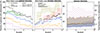 |
Fig. 1. Detection of substructures at a rest-frame wavelength of 1 μm for the entire sample (black) and for three substructure types: clumps (blue), moderately large ones (orange), and extended ones (pink). See Sect. 4.2 for more details. Left: fraction of galaxies with at least one substructure detected with the optimal approach (see Sect. 3.2) as a function of redshift. We show the rest-frame NIR detections carried out by Kalita et al. (2024) (red dashed line) and those in the rest-frame UV by Sattari et al. (2023) (green line and crosses). Middle: same but for the intrinsic detection approach (see Sect. 3.3). We show as a light red line a comparable 2σ detection (kp = 2, see reference) carried out in the rest-frame UV from Ribeiro et al. (2017) and, as a light green line, estimated fractions from the simulations studied in Mandelker et al. (2017, see Appendix D). In both figures on the left-hand side and in the middle, for each sample, we show uncertainties (16th and 84th percentiles) as shaded areas with similar colors. Right: median fraction of flux in substructures as a function of redshift for galaxies with at least one substructure. The uncertainties are shown with a blue shaded area for clumps, a double-dashed orange area for moderately large substructures, a single-dashed pink area for extended substructures, and a black shaded area for the entire sample. |
In the redshift range 1 < z < 2, our fractions are systematically twice as high as those in Fig. 4 of Kalita et al. (2024, see also their Table 1), with between approximately 65% and 80% of galaxies with at least one substructure in this redshift range compared to 40% in their case. This may reflect differences in sample selection and detection methods, particularly their use of a 5σ flux detection threshold which is higher than our value of 2σ. Compared to the rest-frame UV detection of Sattari et al. (2023), our detections in the rest-frame NIR are higher by about 15 percentile points at z < 1.5 but become compatible at higher redshift. Moreover, they find a decrease of the fraction of clumpy galaxies with increasing redshift which is consistent with our results, though our decrease is steeper than theirs. Given that they solely detect clumps and that we consider all types of substructures, this may be due to the stronger role that larger substructures play in our detections at z ≈ 1, as illustrated by the pink and orange lines on the left-hand side of Fig. 1.
4.1.2. Intrinsic detection
The middle panel of Fig. 1 shows the fraction of galaxies with at least one substructure detected using the intrinsic detection approach (black line). At z = 1, we find a fraction of approximately 15%, well below the 80% found with the optimal detection technique. This is due to the fact that this approach forces the detections to be carried out as if the galaxies were at z = 4, thus discarding faint substructures not accessible at higher redshift. Hence, this dramatic drop from 80% to 15% at z = 1 between the two approaches hints at how frequently faint substructures are likely to be missed at high redshift.
From z = 1 to z = 4, we find that the fraction of galaxies with substructures in the rest-frame NIR increases from about 15% to 30%. This is broadly consistent with Ribeiro et al. (2017), who computed a similar fraction in the rest-frame UV for a sample of star-forming galaxies at 2 < z < 4 using HST. However, their approach differs from ours in key ways. First, they detect substructures that can span an area roughly half as large (i.e., down to roughly 0.65 kpc at z = 1.6). Second, they do not account for the effect of angular diameter distance on substructure size. However, this effect is small compared to surface brightness dimming. Finally, they detect substructures at a 2σ flux level at z = 2 while our approach detects them at a similar level at z = 4. Despite such differences, in what follow, Ribeiro et al. (2017) remains our main frame of comparison between the rest-frame UV and NIR given their similar treatment of surface brightness dimming.
These results indicate that substructures in the rest-frame NIR are common in galaxies at 1 < z < 4, similar to what is observed with HST in the rest-frame UV. The right-most panel of Fig. 1 shows the median fraction of rest-frame NIR flux in substructures detected with the intrinsic approach as a function of redshift9. We only consider galaxies with at least one substructure detected using the intrinsic approach, otherwise the median fraction would be null since more than half of the galaxies do not host any substructure. Overall, substructures contribute 3% of the NIR flux, with minimal redshift evolution, which is significantly less than what is seen in the rest-frame UV. Using the optimal detection approach would increase the flux fraction by up to two percentile points, particularly at z ≈ 1. For comparison, Guo et al. (2015) measured an average clump contribution to the rest-frame UV light of 15% at M★ ∼ 109.5 M⊙ and 25% at 1010.5 M⊙ for galaxies at 2 < z < 3. Furthermore, they measure a mild increase with decreasing redshift at the low-mass end with approximately 20% at M★ ∼ 109.5 M⊙ and 1 < z < 2. We note two points. First, they include galaxies without clumps when measuring the contribution of clumps to the rest-frame UV light. Second, they only include clumps contributing over 8% of the rest-frame UV flux, thus excluding faint clumps that resemble local star-forming regions. Therefore, their flux fractions are underestimated with respect to ours and the difference between the rest-frame UV and NIR is likely larger. In conclusion, NIR substructures are as ubiquitous as UV clumps, but their contribution to galaxy light is much weaker.
4.2. Separating substructures in size
In this section, we consider the detection of different types of substructures as a function of redshift for the optimal and intrinsic detection approaches. We split our sample into three size categories that are clumps, moderately large substructures, and extended ones (see Sect. 3.4 for their definitions). We provide in Table 4 the fraction of galaxies with clumps detected with the optimal and intrinsic detection approaches in various redshift bins.
4.2.1. Optimal detection
We present in the left panel of Fig. 1 the fraction of galaxies for each type of substructure detected with the optimal detection technique (clumps in blue, moderately large substructures in orange, extended ones in pink). For each class, we recover a trend similar to Sect. 4.1.1 whereby the fraction of galaxies with a given type of substructure systematically decreases with increasing redshift. Moreover, we find that clumps are much more common (about 60% at z = 1 and 20% at z = 4) than moderately large substructures (about 40% at z = 1 and 8% at z = 4) that are themselves more common than extended substructures (about 23% at z = 1 and 1% at z = 4). By z ≈ 3, very few extended substructure are detected in the optimal detection approach. We note that these quite high fractions of galaxies with clumps are inconsistent with certain simulations (e.g., NIHAO, see Buck et al. 2017) which do not produce substructures in stellar mass maps, but generate many in the UV maps. However, the presence of NIR clumps strongly varies between simulations based on the recipes used to, for instance, model feedback processes, the resolution of the simulations, and the fraction of gas within galaxies (e.g., Perez et al. 2013; Bournaud et al. 2014; Fensch & Bournaud 2021).
4.2.2. Intrinsic detection
For the intrinsic detection approach, trends are different. This is shown in the middle panel of Fig. 1. The detection of moderately large substructures marginally increases with redshift from roughly 5% at z = 1 to 10% at z = 4, while that of extended ones oscillates around 1%. Only the clump population shows an evolution with redshift that is consistent with the total population, increasing from 10% at z = 1 to 25% at z = 4. This is expected since clumps dominate the detection budget (see Fig. A.3). Yet, the contribution of moderately large substructures is non-negligible, especially at low redshift. The rise of rest-frame NIR clump detections with increasing redshift appears consistent with the results found by Ribeiro et al. (2017) in the rest-frame UV. This is likely due to our similar methodologies that take into account the effect of cosmological dimming during the detection process. Still, it is worth noticing that our detections are systematically lower and that our redshift evolution is shallower than theirs. Indeed, they find a rest-frame UV clump fraction of about 27% at z = 1 (a factor of 1.3 above our NIR fraction) and of 57% at z = 4 (a factor of 2.3 above). Similar to Kalita et al. (2024), we do not share a consensus with Ribeiro et al. (2017) on the exact definition of what we call clumps and, therefore, they include in their sample larger substructures than we do, as is illustrated in their Fig. 10. This certainly explains why our fractions in the rest-frame NIR for all types of substructures are closer to theirs in the rest-frame UV than when we are considering clumps alone.
We also compare our detections to predictions from simulations of clumpy galaxies undergoing violent disk instabilities (VDIs) from Mandelker et al. (2017, olive-colored dotted line) in the middle pannel of Fig. 1. These simulations are interesting because they produce giant clumps in a range of stellar mass that is compatible with our detections, with both in situ and ex situ origins, and they provide estimates of the fraction of clumpy galaxies in various stellar mass bins that can be compared to our detections using the intrinsic approach. To have a fair comparison, we recompute the fractions as a function of redshift for a population of galaxies with a similar mass distribution as in our sample using the formalism described in Appendix D. We find the same trend of increasing detections with increasing redshift, however, their values are systematically higher than our clump fractions by roughly 30 percentile points. However, we cannot conclude if this difference is due to the implementation of the physics in the simulations leading to VDIs or to the clump detection technique which is done in the intrinsic 3D stellar distribution in their case and in observed images in ours. To get a proper comparison, one would need to create first JWST/NIRCam mocks of the simulations and then perform the clump detection.
We show in the right panel of Fig. 1 the fraction of flux found in each class of substructures detected with the intrinsic approach. Here, for a given class (clumps, moderately large, or extended), we consider galaxies that have at least one substructure in that class. As expected, extended substructures contain the largest fraction of flux in the NIR with typical values ranging from 3% to 12%, followed by moderately large ones (between 2% and 7.5%), and then clumps (between 1% and 5%). Furthermore, we do not find any redshift evolution for extended and moderately large substructures. While we do find a mild trend for clumps, with the median NIR flux fraction increasing from around 1% at z = 1 to 2.5% at z = 4, it is mostly encompassed within the scatter on the order of 2%. We note that clumps nevertheless dominate the substructure detection budget (as illustrated by the intrinsic detections in Fig. 1). Therefore, even though extended substructures are notably brighter when present, their prevalence is so low that they contribute little to the flux budget in general. In other terms, (i) NIR clumps appear nearly as ubiquitous as UV clumps, (ii) their detection in galaxies similarly increases with increasing redshift, but (iii) their NIR flux is so low that their contribution to the flux budget of their host galaxy is negligible (∼1.5%). This is in sharp contrast with UV clumps that can typically contribute 30% to the UV flux of their host galaxy (e.g., Guo et al. 2015, 2018; Ribeiro et al. 2017). We note that, if these two clump populations are similar, this seems consistent with clumps that are relatively long-lived, though still with a strong UV component, observed in simulations of isolated gas-rich disk galaxies at z ≈ 2 (e.g., Bournaud et al. 2014).
Finally, it is interesting to compare the results for the optimal and intrinsic detections since the optimal approach is supposed to be more efficient at detecting faint substructures. At z = 1, the detection of clumps is about 60% in the optimal case but 10% in the intrinsic case. For extended substructures, it is approximately 23% in the optimal case and 1% in the intrinsic one. This highlights that a large number of faint, and thus probably low-mass, clumps are missed by the intrinsic approach at low redshift. Assuming that a similar population of fainter clumps exists at higher redshift, it shows that our detections are biased to the brightest clumps and that galaxies are certainly even clumpier than they appear. This interpretation is consistent with lensed observations of clumps in the optical and the NIR (e.g., Claeyssens et al. 2023, 2025).
4.3. Detecting substructures across the M★ − SFR plane
In this section, we only consider substructures detected with the intrinsic detection technique since this approach allows us to have an unbiased comparison of substructures across the entire redshift range. Historically, UV clumps have been studied in star-forming galaxies on the MS and in starbursts (e.g., Wuyts et al. 2012; Guo et al. 2015, 2018; Ribeiro et al. 2017; Sattari et al. 2023). Several studies have considered the effect of the host galaxy’s stellar mass on clump statistics (e.g., Guo et al. 2015, 2018) and, indirectly, of the SFR by measuring the fractional UV luminosity in clumps. This also applies to NIR clumps (Kalita et al. 2024, 2025a), though the relationship to the host’s SFR has been little studied (except for the fractional SFR; see Fig. 11 of Kalita et al. 2025b). Furthermore, regarding extended substructures, a few studies have measured the strength of spiral arms as a function of the stellar mass and SFR of the host galaxies (e.g., Yu et al. 2021). In this section, we look at the interplay between the host’s stellar mass and SFR on the presence and properties of NIR substructures.
4.3.1. Fraction of galaxies with substructures
According to Arango-Toro et al. (2025), we identify the MS by selecting galaxies that have a SFR within ±0.3 dex in the relationship from Schreiber et al. (2015). Furthermore, we adopt similar definitions to select starbursts (0.6 dex above the MS), the red sequence (sSFR < 10−11 yr−1, about 2 dex below the MS at z = 1 and 2.5 dex at z = 4), and the green valley (between the MS and the red sequence). We show in Fig. 2 the fraction of galaxies with at least one rest-frame NIR substructure (top row) and one clump (bottom row) detected with the intrinsic detection technique in bins of host galaxy’s stellar mass and SFR. We split our sample into four redshift bins from z = 1 to z = 4, with each step chosen so that it encompasses 1 Gyr of cosmic history. This choice seems a good compromise for three reasons. First, it provides a sufficiently large number of galaxies in each redshift bin to probe different parts of the M★ − SFR plane. Second, the redshift steps are small enough to follow the evolution of the galaxy population and its clumpiness before and after the peak of star formation density at z ≈ 2. And third, it corresponds to the typical migration timescale of long-lived clumps produced in certain simulations (e.g., Bournaud et al. 2011; Dubois et al. 2012). Furthermore, we provide in Fig. A.4 a similar figure using the stellar mass and SFR derived with CIGALE. Overall, even though the stellar masses from CIGALE are above those of LEPHARE and the SFRs slightly below, we recover similar results to those presented below.
First, along the MS and at all redshifts, we observe an increasing number of galaxies with substructures as we move toward higher host’s stellar mass and SFR values. Below 109.75 M⊙ at z < 1.3 and 109.5 M⊙ at z > 1.3, we do not find substructures on the MS. Above 1010.5 M⊙, the fraction of MS galaxies with substructures becomes greater than 70% at all redshifts. Beyond 1010.75 M⊙, nearly all galaxies on the MS have at least one substructure. We find a similar trend for clumps at z < 1.75, with a fraction of galaxies with clumps reaching about 50% at 1010.5 M⊙ and 70% at M★ > 1010.75 M⊙. However, the highest fraction of galaxies with clumps (∼70%) is reached at the high-mass end of the MS at 1.3 < z < 1.75 and then reduces to approximately 50% at z > 1.75. Second, there is a noticeable increase of substructure detections (including clumps) with higher SFRs at a fixed stellar mass, with the highest detection rates reached for starbursts and the high-mass end of the MS. This result appears consistent with measurements of the strength of spiral arms measured in local galaxies selected in the Sloan digital sky survey (SDSS) where stronger arms are found in more star-forming galaxies at a given stellar mass (see Fig. 2 for Yu et al. 2021). Overall, we find higher fractions of galaxies with substructures or clumps at higher stellar masses at a given SFR. Interestingly, this applies for galaxies in the green valley and in the red sequence with, for the latter, the detections ramping up from nearly 0% at the lowest stellar masses to about 40% at M★ > 1010.5 M⊙. Similarly, the fraction of galaxies on the green valley with at least one substructure increases from 0% at M★ ≲ 1010 M⊙ to 100% at M★ ≈ 1011 M⊙. Furthermore, the galaxies at the high-mass end of the green valley behave differently depending on their SFR. Those with the highest SFRs have fractions close to those found on the MS at the same mass. On the other hand, massive galaxies on the green valley with the lowest SFRs have fractions of roughly 50% at z < 2.5 and 60% at z > 2.5, closer to the values found at the high-mass end of the red sequence.
According to Fig. 2, the region where we do not detect any substructures appears mostly independent of redshift. We can define a delimiting line that isolates that region, as illustrated with the dashed line in Fig. 2 whose parametric form is given by:
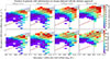 |
Fig. 2. Top row: Median fraction of galaxies with at least one substructure detected with the intrinsic approach as a function of their host galaxy’s stellar mass and SFR in four redshift bins, each spanning roughly 1 Gyr of cosmic time. Bottom row: Same for clumps. Violet corresponds to 0% and red to 100% for substructures (70% for clumps). In each panel, the dashed line isolates the region where no substructure is detected (see Eq. (4)). Galaxies above the blue line are located in the starburst region, those in the hatched region are on the MS from Schreiber et al. (2015) evaluated at the average redshift of each panel, and those below the red line are in the red sequence with sSFR < 10−11 yr−1. We do not show bins with fewer than ten galaxies. |
 (4)
(4)
with x = log10 M★ in M⊙ and y = log10 SFR in M⊙ yr−1. We estimate the uncertainty associated with each bin using bootstrapping (see Sect. 1) and find that the standard deviation of the fraction of galaxies with substructures is on the order of 10 percentile points. Galaxies in the region delimited by Eq. (4) tend to have uncertainties below 2 percentile points. On the other hand, low-mass starbursts as well as galaxies in the green valley and red sequence with M★ ≳ 1010.5 M⊙ have a higher uncertainty of 15 percentiles points, with a few bins reaching 25 percentiles points.
It is expected from the mass-size relationship (e.g., Martorano et al. 2024) that the size and compactness of the host galaxies depend on their stellar mass and SFR. Lower-mass galaxies and/or with lower SFR should be smaller, thus reducing the area over which clumps are detected (as illustrated in Fig. A.2) and may disfavor small galaxies compared to extended ones. We have checked for this effect by reproducing Fig. 2 in five bins of global effective radius (see Eq. (6) of Mercier et al. 2022): Reff < 1.08 kpc, 1.08 < Reff/kpc < 1.61, 1.61 < Reff/kpc < 2.22, 2.22 < Reff/kpc < 3.17, and Reff > 3.17 kpc. These bins are chosen so that they contain 20% of the galaxies. We find that, whatever the size bin, we always recover Eq. (4) meaning that the part of the M★ − SFR plane that is devoid of substructures is not biased by the size of the galaxies. The high-mass end of the red sequence (M★ > 1010.5 M⊙) is dominated by small (Reff < 1.61 kpc) and therefore compact galaxies, which goes against a size bias. However, the variation of the fraction of galaxies with substructures or clumps visible along the MS and the starburst region seen at M★ ≳ 1010 M⊙ in Fig. 2 becomes prominent at Reff > 1.61 kpc and is dominated by large galaxies (Reff > 2.2 kpc). Furthermore, massive galaxies in the green valley behave similar to those on the MS at the same mass. Therefore, this may bias our substructure and clump detections at the high-mass and high-SFR ends by favoring the most massive galaxies with the highest SFRs. To control for this effect, we reproduce Fig. 2 but weighting each substructure detection by the area over which it is carried out, as illustrated in Fig. A.5. We find that we recover comparable results as when not weighting the detections, which shows that our results are not produced by a galaxy size bias but appear as a genuine stellar mass and SFR dependence. We note that the lack of detections in the region delimited by Eq. (4) is likely not intrinsic but an observational effect. If we compare our detections in the lowest redshift bin using the intrinsic and optimal detection techniques, we see that the delimiting line given by Eq. (4) moves toward galaxy hosts with lower stellar mass and SFR values. In other terms, low-mass and low-SFR galaxies are likely to host substructures that are too faint to be detectable with the intrinsic detection method. We do not consider such substructures in what follows because we cannot observe them at higher redshift.
Galaxies with low SFR values tend to host lower amounts of cold gas which should lead to less fragmentation and fainter clumps. Therefore, assuming that substructures are mainly formed through disk fragmentation (see Sect. 5.4 for a discussion), we actually expect the region delimited by Eq. (4) to be mostly devoid of relatively bright substructures. The transition at M★ > 1010.5 M⊙ could typically be due to galaxy mergers and fast quenching channels rapidly moving galaxies from the starburst region and MS to the green valley and red sequence while retaining previously formed clumps and producing features such as tidal tails and merger remnants. A detailed analysis of the star formation history of the galaxy hosts and comparisons to high-resolution simulations of realistic galaxies in their environment would be key to test that assumption.
Linear correlation between the fraction of rest-frame NIR flux in substructures or clumps and the sSFR and partial correlation between the flux fraction and (i) the stellar mass of the host galaxy at a fixed host’s SFR, and (ii) the SFR of the host galaxy at a fixed host’s stellar mass.
4.3.2. Flux in substructures
We consider the total fraction of rest-frame NIR flux in substructures and clumps detected with the intrinsic detection approach across the M★ − SFR plane. This is shown in Fig. 3 for galaxies that host at least one substructure (top row) or one clump (bottom row) and for stellar mass and SFR bins containing at least ten galaxies. Therefore, Fig. 3 is limited to galaxies on the MS, in the starburst region, and at the high-mass and high-SFR ends of the green valley. Alternatively, we also show in Fig. A.6 the median fraction of rest-frame NIR flux in substructures or clumps as a function of the host galaxy’s stellar mass, color coded in bins of host galaxy’s SFR. The difference between Figs. 3 and A.6 is that the latter also highlights the scatter around the median value for populations of galaxies with different star formation levels.
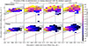 |
Fig. 3. Same as Fig. 2 but representing the fraction of flux in substructures (top row) or clumps (bottom row) detected using the intrinsic detection approach in each galaxy host’s stellar mass and SFR bin. To compute the fraction of flux we consider only those galaxies that contain at least one substructure. |
The brightest substructures at z > 1.3 are found in the starburst region throughout the entire stellar mass range. They typically host 4% of the total rest-frame NIR flux of the galaxies, with fractions oscillating between approximately 2% and 10% at M★ ≈ 109 M⊙ and between 2% and 7.5% at higher stellar masses. From Fig. 3, it looks like stellar mass is loosely correlated with the flux fraction and that galaxies with a lower SFR have a lower fraction of their rest-frame NIR flux in substructures. Indeed, the lowest flux fraction, equal to 0.5%, is reached at 1.75 < z < 2.5 at the limit between the high-mass ends of the green valley and the red sequence. We estimate the partial correlation between the rest-frame NIR flux fraction and (i) the galaxy host’s stellar mass at fixed host’s SFR and (ii) the host’ SFR at fixed host’s stellar mass. In addition, we consider the correlation between the rest-frame NIR flux fraction and the sSFR of the host galaxies. The values of the (partial) correlations computed in four redshift bins using the linear Pearson coefficient and the nonlinear Spearman coefficient are presented in Table 5. Overall, we find low correlations between the rest-frame NIR flux fraction in substructures and the three aforementioned galaxy host’s physical parameters. At 1 < z < 1.3, the flux fraction is loosely anticorrelated with stellar mass (Pearson coefficient of r ≈ −0.15) but, at higher redshift, the correlation vanishes and the flux fraction becomes loosely correlated with SFR (r ≈ 0.15) instead. At any redshift, there is also a weak correlation with sSFR (r ≈ 0.15). This means that more star-forming galaxies are likely to contain more of their rest-frame NIR flux in substructures. This is consistent with starbursts having the highest fractions, as previously mentioned.
Interestingly, the trends found for clumps are different, with the highest rest-frame NIR median flux fraction (about 4%) reached in the low-mass part of the MS and starburst region (M★ < 109.5 M⊙). The fraction decreases with increasing galaxy host’s stellar mass and SFR, reaching a median value of less than 0.5% at M★ ∼ 1011 M⊙ on the MS, starburst region, and green valley. Similar to substructures, we derive the correlation with the host galaxies’ sSFR and the partial correlations with stellar mass and SFR. We find a negligible anticorrelation between the median clump flux fraction and the galaxy host’s SFR but a much stronger anticorrelation with the stellar mass (r ≈ −0.5). There is also a weaker positive correlation with the host’s sSFR (r ≈ 0.23) but the stellar mass remains the physical parameter that is the most strongly correlated. This is consistent with clumps in massive galaxies contributing less to the rest-frame NIR flux budget than in lower-mass galaxies. We note that this corresponds to a mild evolution of the stellar mass found in clumps with the galaxy host’s stellar mass. Assuming similar mass-to-light ratios between the clumps and the host galaxies, a flux fraction of 4% at M★ = 109.5 M⊙ corresponds to a total clump stellar mass of roughly 108 M⊙, while 1% at M★ = 1011 M⊙ corresponds to a total clump stellar mass of roughly 5 × 10⁸ M⊙.
If we use the nonparametric Spearman correlation instead, we find the same trends for both clumps and substructures with, generally speaking, correlations stronger by 20%. This should be taken as an indication that the fraction of flux in substructures and clumps in the rest-frame NIR is not linearly correlated to the galaxy host’s stellar mass, SFR, and sSFR. Furthermore, we note that, in either case, we do not find an evolution of the correlations with redshift. The different correlations with the stellar mass and SFR of the host galaxy observed between all types of substructures and clumps show that the flux contribution of moderately large and extended substructures behave differently from clumps and are more strongly correlated with SFR and sSFR than with stellar mass. We note that this behavior appears consistent with the results from Yu et al. (2021) where they find stronger spiral arms in galaxies with higher SFR values, but no dependence on the galaxy host’s stellar mass.
5. Discussion
5.1. Interpretation about the evolution of clumpiness with redshift
Figure 4 shows the redshift evolution of the fraction of galaxies with substructures (left panel) and clumps (middle panel) in different regions of the M★ − SFR plane, as illustrated in the right panel. Overall, we observe no noticeable trend, with the fraction of galaxies with clumps or substructures at a given location in the M★ − SFR remaining roughly constant with redshift. The observed fluctuations between redshift bins, typically ten percentile points, are within the uncertainties. There are, however, two regions at the high-mass end of the green valley (M★ = 1011 M⊙) with log10(SFR/M⊙ yr−1) = 0.15 and 0.75 that show a measurable decrease with redshift going from approximately 60% and 75% at z = 4 to 50% and 35% at z = 1, respectively. In each case, the decrease becomes notable with cosmic time starting from z ≈ 2. This corresponds to the peak of star formation and may reflect morphological transformations as massive galaxies quench and pass through the green valley.
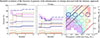 |
Fig. 4. Evolution of the fraction of galaxies with substructures (left panel) and clumps (middle panel) detected with the intrinsic detection approach as a function of redshift for different regions of the M★ − SFR plane, as illustrated in the right panel with circles of a different color, line style, and thickness. We use the same redshift bins spanning 1 Gyr of cosmic time as in Figs. 2 and 3. Each circular region has a radius of 0.2 dex and the regions are chosen to evenly map the plane. We only show regions with more than ten galaxies in all redshift bins and lines are slightly offset vertically to improve readability. |
These results may appear to contradict the redshift evolution described in Sects. 4.1 and 4.2 but it can be explained in two complementary ways. First, over cosmic time, the green valley and red sequence build up, both with lower fractions of galaxies with substructures than the MS or starburst region. This is particularly true in the low-mass regime (M★ < 1010.5 M⊙), where we detect no substructure. Second, galaxies on the MS and starbursts evolve with cosmic time, both moving toward lower SFRs at a given stellar mass. Therefore, this leads overall to lower fractions of galaxies with substructures or clumps.
These two effects are illustrated in Fig. 5 where we see that the fraction of clumpy galaxies on the MS and in the starburst region both increase at least by a factor two from z = 1 to z = 4. In practice, the likelihood of a galaxy hosting substructures depends on its evolutionary track in the M★ − SFR plane. For instance, a galaxy starting with low stellar mass and SFR values and building up its mass by moving toward the MS or the starburst region is more likely to host substructures at a later stage. Conversely, a low-mass galaxy at z = 4 in the starburst region likely hosts substructures. If it builds mass at a constant SFR and quenches at M★ ≲ 1010.5 M⊙, it must become smoother over time. However, if it quenches at M★ ≳ 1010.5 M⊙, we do not expect all substructures to disappear, though, according to Fig. 3, they should become fainter with cosmic time.
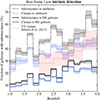 |
Fig. 5. Intrinsic detection of substructures (black) and clumps (blue) for galaxies on the MS (continuous lines) and for starbursts (dotted lines) as a function of redshift. For comparison, we also show the rest-frame UV detections from Ribeiro et al. (2017, light red). Shaded areas correspond to the uncertainties computed as the 16th and 84th percentiles. |
5.2. Impact of young stellar populations
The strong correlation between the clumpiness of the galaxy population and the SFR of the host galaxies raises the question of whether rest-frame NIR substructures in galaxies with high SFR values could be the result of young stellar populations. This could also explain the higher fractions of fluxes seen in Fig. 2. We devise a toy model to check for this effect by assuming that substructures have been formed through a recent burst of star formation, so that the impact of young stellar populations in the rest-frame NIR is maximal. We can split the rest-frame NIR flux of the host galaxy into an old component Fo = M★/Υ★, with Υ★ the mass-to-light ratio for the old stars, and a young one with Fy = αy × SFR where αy is the SFR-to-flux conversion factor. The old component scales with M★ because its flux is produced by the accumulation of old stars from its past star formation history while the young component is short-lived and, thus, must scale with the SFR. On the other hand, substructures are made of young low- and high-mass stars whose flux, by construction, must scale with the SFR as Fy = αy × CSFR × SFR, where CSFR is the fraction of SFR found in substructures. Let us note η = Fs/(Fo + Fy) the fraction of rest-frame NIR flux in substructures, so that we have
 (5)
(5)
If the fraction of SFR in substructures (CSFR) is constant, Eq. (5) shows that η should increase with the sSFR of the host galaxy. Similarly, if CSFR increases with the sSFR (starbursts and galaxies in the MS are more likely to develop instabilities and produce clumpy star formation), we expect η to increase with the sSFR. This is what we see qualitatively in Fig. 3 for substructures and measure as a weak correlation in Table 5. For clumps, we find a slightly stronger correlation with the sSFR but, as already mentioned, the fraction of rest-frame NIR flux in clumps is much more strongly anticorrelated with the stellar mass of the host galaxy than its sSFR. We note that Eq. (5) should be rewritten as η = Fs/(Fo + Fy + Fs) for the most extended substructures since they can typically contribute to 5% of the rest-frame NIR flux (sometimes up to 12%; see the right panel of Fig. 1). For this type of substructures, the net effect is that an increase in CSFR produces a shallower growth of η than for clumps.
As noted previously, the fraction of rest-frame NIR flux in clumps decreases with increasing stellar mass at a given sSFR. If we interpret this in light of Eq. (5), this would mean that CSFR would have to decrease with increasing stellar mass at a given SFR or sSFR, as is visible in Fig. 3. For instance, for galaxies in the MS at z ≈ 1.5, this would require CSFR to decrease by a factor of roughly 2.5 from M★ = 109.75 M⊙ to 1010.75 M⊙. Such a variation of CSFR with the stellar mass of the host galaxy appears inconsistent with measurements of rest-frame UV clumps. For instance, in Guo et al. (2015), they find a contribution of UV clumps to the SFR between 5% and 10% without any significant difference between galaxies in the stellar mass range 109 < M★/M⊙ < 1011.4. Thus, it seems that a young stellar component cannot explain alone the fraction of NIR flux observed in clumps unless CSFR is anticorrelated with the stellar mass of the galaxy host.
5.3. Characteristics of multiclump systems
We compare the physical properties of galaxies hosting a single clump with those hosting multiple clumps. The interested reader can find a similar discussion for rest-frame UV clumps in Ribeiro et al. (2017). They find that about 25% of their sample of star-forming galaxies is made of two-clump systems and favor major mergers as the main formation channel for such systems. However, we note that our definitions of clumps are different (see Sects. 4.1.2 and 4.2.2 for some of the key differences) which means that a direct comparison is not possible. Notably, they can detect the central bulge as a clump whereas we exclude it from our detections. The difficulty in comparing stems from the fact that the rest-frame UV is much more heavily affected by dust attenuation. It is therefore not clear how frequently the central bulge is detected as a clump in their analysis. This is important because if the bulge is detected as a clump in most cases, we should compare their two-clump systems to our single-clump systems. Otherwise, their two-clump systems are similar to ours and a direct comparison is possible.
To simplify the interpretation, we split the sample into starbursts, galaxies on the MS, in the green valley, and in the red sequence. We exclude galaxies within the region delimited by Eq. (4) since we do not find substructures in such galaxies. We show in Fig. 6 the average probability (and its standard deviation) to find exactly one clump (continuous lines) or two or more clumps (dashed lines) for a given type of galaxy and a given stellar mass in four redshift bins spanning each roughly 1 Gyr of cosmic time. We consider galaxies for which we detect at least one clump to compute the average probability using Eqs. (C.6) and (C.8). The probabilities of having one and two or more clumps do not sum to 100% because galaxies also have a nonzero probability of hosting no clump. We note that if we select galaxies with at least one clump by using a cut on the probability Pr{N ≥ 1} (see Appendix C for the notation) we recover the same trends.
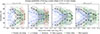 |
Fig. 6. Average probability that a galaxy of a given stellar mass with at least one clump hosts either a single clump (continuous lines) or two or more clumps (dashed lines) for starbursts (blue circles), galaxies on the MS (black squares), in the green valley (green diamonds), and in the red sequence (red crosses). For each class, we show the standard deviation of the probability as a semitransparent filled area with a similar color. The probabilities are computed using Eqs. (C.6) and (C.8). |
Whatever the redshift, stellar mass, and type of the galaxy host, the population of clumpy galaxies is dominated by galaxies hosting a single clump. In the low-mass regime (M★ = 109.5 M⊙), the probability is higher in the MS (about 85%) than in the starburst region (about 60%). We do not see a strong variation with redshift, except at 2.5 < z < 4 where the probabilities for galaxies on the MS and in the starburst region are both equal to approximately 80%. At higher stellar masses and for all galaxy types, the probability to find a single clump in a clumpy galaxy decreases, reaching 60% at z > 1.3 and M★ ≈ 1010.5 M⊙ for starbursts and galaxies on the MS. For galaxies on the MS at M★ ≥ 1011 M⊙, the probability to have a single clump reduces to nearly 50%. Furthermore, we find that the probability that galaxies in the green valley have a single clump is systematically above that of galaxies on the MS. For instance, at 1 < z < 1.3, galaxies on the green valley with M★ ≈ 1010.5 M⊙ have a probability of roughly 75% while those on the MS have 55%. Similarly, massive galaxies in the red sequence (M★ > 1010.5 M⊙) systematically have a higher probability to host a single clump than other types of galaxies.
A consequence of looking at the population of clumpy galaxies is that if the probability of hosting a single clump decreases with stellar mass, then the probability of hosting two or more clumps must evolve in the opposite way. This is what we find in Fig. 6. Whatever the redshift, the probability to find a clumpy galaxy with multiple clumps is below 10% for galaxies on the MS and in the green valley at low stellar masses (M★ < 1010 M⊙). In this mass range, starbursts are the only galaxies with a non-negligible probability (∼30%) to have two or more clumps. Whatever the type of galaxy, the probability to find two or more clumps strongly increases with the host’s stellar mass, reaching values as high as 40% at the high-mass end of the MS and the green valley. Even, galaxies on the red sequence at z < 1.3 have a probability close to 50% to host two or more clumps.
We further check whether it is more probable for galaxies to host exactly two clumps. For galaxies in the red sequence, we find that the majority of multiclump systems host exactly two clumps. For starbursts and galaxies on the MS and in the green valley, we find that the probability to find exactly two clumps is close to the values presented in Fig. 6, on average reduced by ten percentile points. This means that massive starbursts and galaxies on the MS have a probability to host exactly two clumps between 20% and 30% which is consistent with the fraction of galaxies with exactly two rest-frame UV clumps derived by Ribeiro et al. (2017). Therefore, single-clump systems dominate the population of both star-forming and quiescent galaxies at all redshifts and stellar masses. Multiclump systems (including mostly two-clump ones) are nevertheless non-negligible. They are more commonly found in star-forming galaxies than in quiescent ones and they contribute more importantly to the clumpy population at higher stellar masses, in particular at the high-mass end of the MS and green valley.
5.4. Interpreting the origin of rest-frame NIR substructures
Two major pathways regarding the origin of giant clumps in high-redshift galaxies are typically discussed. On the one hand, clumps could be produced by local disk fragmentation in turbulent and gas-rich disks (e.g., Elmegreen 2006; Genzel et al. 2008, 2011). If clumps can survive over sufficiently long timescales (typically 1 Gyr or above), their rest-frame NIR flux would decouple from the current SFR of their host galaxy. This would explain the lack of correlation between the fraction of rest-frame NIR flux measured in flux clumps and the galaxy host’s SFR, as discussed in Sect. 4.3.2. Furthermore, the fact that massive galaxies with high SFR values (SFR ≳ 10 M⊙ yr−1) are the most likely to host multiple clumps is also expected from disk fragmentation. However, we note that certain simulations (e.g., Bournaud et al. 2014) suggest that the old stellar component of long-lived giant clumps is partially disrupted by tidal stripping while a young stellar component is continuously replenished by star formation. In such a case, we would expect to see come correlation with the SFR of the galaxy host.
On the other hand, the observed clumps could be the remnants of past galaxy minor (e.g., Guo et al. 2015) or major mergers (e.g., Ribeiro et al. 2017). This would be consistent with clumpy galaxies hosting usually a single clump that would correspond to the surviving core of the secondary galaxy that has merged. However, depending on the typical merging timescale, the frequency of mergers, and on the migration timescale of the remaining core within the primary galaxy, we may expect to detect multiple cores as clumps. Therefore, the existence of multiclump systems does not necessarily favor fragmentation over galaxy mergers as the main formation channel for clumps. In addition, we expect galaxy mergers and fly-byes to produce tidal features that we may detect as extended substructures. If we believe that galaxy mergers produce a significant fraction of starbursts (e.g., Faisst et al. 2025), then we would expect extended substructures to dominate in that population. This appears to be consistent with Fig. 3 in which we see that the fraction of rest-frame NIR flux in substructures peaks in the starburst region, but not for clumps, thus showing that extended substructures dominate the flux budget in that population of galaxies. Nevertheless, we note that extended substructures do not have to be tidal tails but, instead, could be bars and spiral arms produced by density waves or stochastic clumpy star formation, as suggested by Kalita et al. (2025c).
Disentangling between clumps formed in situ (i.e., fragmentation) and ex situ (i.e., mergers) is not trivial. One way to determine which origin is more likely is by looking at the spatial distribution of clumps. Indeed, clumps produced via disk fragmentation should be formed and then migrate inside the stellar disk. On the other hand, if the rest-frame NIR clumps trace galaxy mergers, we expect to find a significant fraction of them outside of the plane of the disk component of the galaxy. We use clumpy edge-on galaxies to study the spatial distribution of clumps. We select the subsample by requiring that the galaxies have a stellar disk axis ratio b/a < 0.15, with b and a the minor and major axes, respectively, and a bulge-to-total rest-frame NIR flux ratio B/D < 0.5. The latter criterion is necessary to ensure selecting galaxies that host a disk component that is bright enough, otherwise the stellar disk axis ratio would become loosely constrained. This yields a subsample of 85 clumpy edge-on galaxies, more than 80% of which are starbursts or on the MS. Finding substructures in edge-on galaxies is biased because we detect them within the extent of the segmentation maps produced by SEXTRACTOR++. Since the segmentation maps tend to follow the shape of the galaxies, this disfavors detecting substructures along the minor axis if they are located sufficiently far from the disk plane. In turn, this can give the impression that substructures are located preferentially within the plane of the disk. Luckily, if a substructure located outside of the disk plane is not associated to the segmentation map of the galaxy, that means it was detected as a separate galaxy by SEXTRACTOR++. Therefore, we can use the COSMOS2025 catalog from Shuntov et al. (2025a) to search for nearby companions to edge-on galaxies and include them in our analysis. To get companions comparable to substructures, we require that (i) they are located at most 3 arcsec away from the center of the main galaxy10, (ii) their photometric redshift is within 1σ of the redshift of the main galaxy, and (iii) their contribution to the rest-frame NIR flux is at most 15%. The latter criterion is used to remove galaxy companions that are too bright to be consistent with the fluxes measured in Sect. 4.3.2. With this criterion, the median rest-frame NIR flux fraction in companions is roughly 5%, with the 16th and 84th percentiles equal to 1.75% and 10%, respectively.
We show in Fig. 7 the spatial distribution of substructures detected with the intrinsic detection method (circles) and galaxy companions (crosses) color-coded by the redshift of the host galaxy. Along the x axis, we represent the distance to the center of the galaxy and, along the y axis, the angle between the barycenter of the clump (or companion) and the major axis of the host, modulo 90°. We do not separate between clumps, moderately large, and extended substructures because they are distributed similarly. Since a given physical distance can carry different meanings depending on the size of the galaxies, we provide in Fig. A.7 a similar figure but with the distance to the center normalized by the scale length of the stellar disk11.
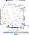 |
Fig. 7. Position of intrinsic substructures (circles) with respect to the galaxy host color-coded with redshift. The detection is done in edge-on galaxies with bulges contributing less than 50% to the rest-frame NIR flux. We show on the x axis the distance to the center of the host galaxy and, on the y axis, the angle between the barycenter of the substructure and the major axis of the host galaxy. Crosses show the distribution of galaxy companions with properties comparable to clumps, selected at a distance below 3 arcsec from the galaxy, with a total flux in the rest-frame NIR below 15%, and within 1σ of the redshift of the main galaxy. Pink dotted lines represent isocontours of the vertical distance to the galaxy plane. |
We find that half of substructures are located closer than 3.5° from the disk plane, and 75% are closer than 10°. Furthermore, half of them are located less than 3.5 kpc away from the center of their host galaxy and 75% are within approximately 6 kpc12. If we measure the vertical distance of substructures with respect to the plane of the stellar disk, we find that half of substructures are closer than 250 pc and 75% are below 650 pc. This latter distance is close to the scale-height measurements of disk galaxies at z ≈ 1, approximately equal to 500 pc (e.g., Usachev et al. 2024). In other terms, the majority of substructures detected in edge-on galaxies appear to be located within the plane of the stellar disk. We note that the distributions of substructures above and below z = 3 are different. At high-redshift, substructures appear closer to the center of the galaxy and about 25% of them are distributed with an angle larger than 30° (8% at z < 3) and with a vertical distance ranging from 500 pc to 2 kpc. Interestingly, when normalizing the distance by the scale length of the stellar disk, the difference between low and high redshift becomes less clear, with a median distance of 1.5Rd and the 16th and 84th percentiles equal to 0.6Rd and 2.6Rd, respectively. There is however a population of substructures in galaxies at z > 2 that are found both at small (< 0.5Rd) and large distances (5Rd) and that we do not find at lower redshift. On the other hand, galaxy companions are distributed relatively evenly in terms of angle which confirms the hypothesis that if galaxy mergers produce clumps, they should be distributed in all directions. Furthermore, companions are located at large distances, typically beyond 5 kpc from the center, at R > 5Rd, and at large vertical distances, with 80% of them beyond 5 kpc.
There is a region in Fig. 7 between approximately 2 kpc and 5 kpc above the plane of the stellar disk where very few substructures and companions are found. This could be a dynamical effect due to the nature of mergers. If the secondary galaxies have eccentric orbits, they are expected to spend more time close to their apocenter where they would be detected as companions located at large distances. On the other hand, during their last phase of merger, if they merge in an orbit that is not coplanar with the stellar disk of the main galaxy, they would be identified as substructures close to the center and with a large angle. However, we note that it is possible that, after a few orbits, the dynamical interactions between the two galaxies bring the galaxy companion into the stellar disk plane, in which case the merger remnants would be identified as substructures. Since roughly 11% of edge-on galaxies have at least one companion in a shell between 10 kpc and 30 kpc, we can estimate the fraction of companions that would end up detected as substructures between 1 kpc and 10 kpc if they all move into the stellar disk. We find that about 1.5% of edge-on galaxies would host a merger companion detected as a clump. In comparison, when combining all redshift ranges, we find that 21% of edge-on galaxies host at least one substructure. Therefore, galaxy mergers do not seem to be the driving mechanism behind the formation of substructures in galaxies. On the other hand, local disk fragmentation is a much more likely scenario. This conclusion is consistent with Huertas-Company et al. (2020) for clumps detected in the rest-frame UV and optical and with Zanella et al. (2019) for compact UV clumps detected at similar redshifts with HST.
6. Conclusion
We have studied substructures at a rest-frame wavelength of 1 μm in galaxies at 1 < z < 4 with M★ > 109 M⊙ in the COSMOS-Web survey by identifying contiguous substructures in residual images from the JWST/NIRCam F277W and F444W bands, following the removal of an axially symmetric bulge-disk model. We have used two distinct methods: (i) an optimal approach detecting all substructures above a given flux level and (ii) an intrinsic approach applying redshift-dependent surface and flux thresholds to correct for cosmological biases. Each approach detects small substructures (i.e., clumps), moderately large ones, and extended ones. The optimal detection approach yields the following results.
-
(i)
Rest-frame NIR substructures are ubiquitous in galaxies at z = 1 and are present in half of them at z = 4.
-
(ii)
Clumps are the most common substructures at all redshifts, though extended substructures are found in approximately 20% of galaxies at z = 1 (a few percents at z = 4).
We note that the optimal detection approach does not detect substructures of comparable size and luminosity across redshifts, thus biasing our results. However, the intrinsic approach corrects for the redshift dependence of substructure size and flux. This approach yields the following results.
-
(i)
The galaxy population has become less clumpy over cosmic time, with the fraction of galaxies with substructures going from about 40% at z = 4 to 10% at z = 1.
-
(ii)
Clumps are the most common substructures at all redshifts, even though moderately large substructures contribute to about half at z = 1. And
-
(iii)
substructures contribute a small fraction of rest-frame NIR flux (1% for clumps, 3% for moderately large substructures, 5% for extended substructures) compared to the rest-frame UV flux, as quoted in the literature (usually more than 30%). Furthermore, we do not find a redshift evolution.
Since our sample comprises both star-forming and quiescent galaxies, we have checked in which population substructures are more likely to be located by looking at the prevalence of substructures and their fraction of flux in the rest-frame NIR across the M★ − SFR plane. We find the following.
-
(i)
Rest-frame NIR substructures are absent in galaxies with low stellar mass and SFR (M★ ≲ 1010.5 M⊙ and SFR ≲ 10 M⊙ yr−1).
-
(ii)
Substructures are ubiquitous in massive galaxies (M★ ≳ 1010 M⊙) on the MS, in the starburst region and at the high-SFR end of the green valley. Similarly, approximately 70% of that population of galaxies hosts at least one clump.
-
(iii)
The brightest substructures (approximately 4% of the rest-frame NIR flux) are found in galaxies with the highest sSFR values and the faintest ones are found at the high-mass end the red sequence. However, the brightest clumps are found in low-mass galaxies (M★ ≈ 109 M⊙) and the faintest clumps are found in the most massive galaxies on the MS, starburst region, and green valley. And
-
(iv)
at a given location in the M★ − SFR plane, the fraction of galaxies with substructures or clumps shows no significant redshift evolution. One exception is at the low-SFR end of the green valley, near the transition to the red sequence, where the fraction galaxies with substructures has dropped by 20 percentile points from z = 4 to z = 1.
We conclude that, regardless of redshift, the clumpiness of the galaxy population in the rest-frame NIR depends on both the stellar mass and SFR of the host galaxies. Thus, galaxies evolving along the MS or reaching the starburst region are more likely to develop substructures such as clumps. On the other hand, galaxies in the process of quenching are less likely to retain substructures. We attribute the decline in clumpy galaxies over cosmic time to the evolution of the galaxy population toward lower SFR values and to the buildup of the low-mass green valley and red sequence after the peak of star formation at z ≈ 2.
Clumpy galaxies are more likely to host a single clump. This is especially true at low stellar masses (M★ < 1010 M⊙) where clumpy galaxies on the MS have a 80% probability of hosting a single clump (between 60% and 80% for starbursts). This implies that low-mass starbursts are more likely to host multiple clumps (30% probability) than galaxies on the MS (a few percent). Moreover, we find that massive clumpy galaxies are more likely to host multiple clumps, up to 40% at M★ ≈ 1011 M⊙ for those on the MS and in the green valley.
The spatial distribution of rest-frame NIR substructures in edge-on galaxies shows that they are mostly located close to the stellar disk plane. This spatial distribution is consistent with local disk fragmentation but could also result from galaxy mergers if the merger remnants preferentially settle in the disk. We use detections of nearby galaxy companions, with properties similar to detected substructures, to estimate the fraction of substructures potentially resulting from past galaxy mergers. Overall, galaxy mergers cannot account for most substructures. Thus, local disk fragmentation is the most plausible formation mechanism for rest-frame NIR substructures, especially clumps.
We note that this conclusion only applies to disk galaxies. Therefore, clumps found in other populations could still be produced ex situ. In particular, this could be the case for clumpy galaxies at the high-mass end of the red sequence that tend to host a single clump in the majority of cases. More detailed studies of substructures in different populations of galaxies are required to understand their origin. In particular, one could (i) evaluate the physical properties of substructures using SED modeling (e.g., stellar mass, SFR, or age) and correlate them to the characteristics of their host galaxy (for an attempt and discussions therein, see Claeyssens et al. 2023, 2025; Kalita et al. 2025a,b), (ii) study the presence and properties of substructures as a function of the SFH of their galaxy host. Typically, this could be used to put constraints on the survivability timescale of clumps. And (iii) one could compare our detections of substructures with mocks COSMOS-Web observations produced from simulations to better constrain the physics leading to the formation of realistic rest-frame NIR clumps and substructures.
Data availability
The catalogs containing the selected galaxies and the substructure detections are available at the CDS via https://cdsarc.cds.unistra.fr/viz-bin/cat/J/A+A/706/A136. A notebook showing how to use the catalogs is also available at https://wilfriedmercier.github.io/clump_finder/notebook/catalogue.html.
Acknowledgments
This research is based in part on observations made with the NASA/ESA Hubble Space Telescope obtained from the Space Telescope Science Institute, which is operated by the Association of Universities for Research in Astronomy, Inc., under NASA contract NAS 5–26555. These observations are associated with programs #9822 and #10092. This work is based in part on observations made with the NASA/ESA/CSA James Webb Space Telescope. They can be obtained from the Mikulski Archive for Space Telescopes at the Space Telescope Science Institute, which is operated by the Association of Universities for Research in Astronomy, Inc., under NASA contract NAS 5-03127 for JWST. These observations are associated with program #1727. This work made use of python and the following packages: sqlite3 (Hipp 2020), NumPy (Harris et al. 2020), Matplotlib (Hunter 2007), tqdm (da Costa-Luis et al. 2024), joblib (https://joblib.readthedocs.io/en/stable/), scikit-image (van der Walt et al. 2014), scipy (Virtanen et al. 2020), pingouin (Vallat 2018), Astropy (Astropy Collaboration 2022), and its affiliated package Regions (Bradley et al. 2024). This research is also partly supported by the Centre National d’Etudes Spatiales (CNES). We acknowledge the funding of the French Agence Nationale de la Recherche for the project iMAGE (grant ANR-22-CE31-0007). We warmly acknowledge the contributions of the entire COSMOS collaboration consisting of more than 100 scientists. The HST-COSMOS program was supported through NASA grant HST-GO-09822. More information on the COSMOS survey is available at https://cosmos.astro.caltech.edu. This work was made possible by utilizing the CANDIDE cluster at the Institut d’Astrophysique de Paris, which was funded through grants from the PNCG, CNES, DIM-ACAV, and the Cosmic Dawn Center and maintained by S. Rouberol.
References
- Adamo, A., Östlin, G., Bastian, N., et al. 2013, ApJ, 766, 105 [NASA ADS] [CrossRef] [Google Scholar]
- Aihara, H., AlSayyad, Y., Ando, M., et al. 2022, PASJ, 74, 247 [NASA ADS] [CrossRef] [Google Scholar]
- Arango-Toro, R. C., Ciesla, L., Ilbert, O., et al. 2023, A&A, 675, A126 [NASA ADS] [CrossRef] [EDP Sciences] [Google Scholar]
- Arango-Toro, R. C., Ilbert, O., Ciesla, L., et al. 2025, A&A, 696, A159 [NASA ADS] [CrossRef] [EDP Sciences] [Google Scholar]
- Arnouts, S., Moscardini, L., Vanzella, E., et al. 2002, MNRAS, 329, 355 [Google Scholar]
- Arnouts, S., Le Floc’h, E., Chevallard, J., et al. 2013, A&A, 558, A67 [NASA ADS] [CrossRef] [EDP Sciences] [Google Scholar]
- Astropy Collaboration (Price-Whelan, A. M., et al.) 2022, ApJ, 935, 167 [NASA ADS] [CrossRef] [Google Scholar]
- Bertin, E. 2011, in Astronomical Data Analysis Software and Systems XX, eds. I. N. Evans, A. Accomazzi, D. J. Mink, & A. H. Rots, ASP Conf. Ser., 442, 435 [Google Scholar]
- Bertin, E., Schefer, M., Apostolakos, N., et al. 2020, in Astronomical Data Analysis Software and Systems XXIX, eds. R. Pizzo, E. R. Deul, J. D. Mol, J. de Plaa, & H. Verkouter, ASP Conf. Ser., 527, 461 [NASA ADS] [Google Scholar]
- Boissier, S., & Junais. 2019, in SF2A-2019: Proceedings of the Annual Meeting of the French Society of Astronomy and Astrophysics, eds. P. Di Matteo, O. Creevey, A. Crida, et al. [Google Scholar]
- Boquien, M., Burgarella, D., Roehlly, Y., et al. 2019, A&A, 622, A103 [NASA ADS] [CrossRef] [EDP Sciences] [Google Scholar]
- Bournaud, F., Dekel, A., Teyssier, R., et al. 2011, ApJ, 741, L33 [NASA ADS] [CrossRef] [Google Scholar]
- Bournaud, F., Perret, V., Renaud, F., et al. 2014, ApJ, 780, 57 [Google Scholar]
- Bradley, L., Deil, C., Ginsburg, A., et al. 2024, https://doi.org/10.5281/zenodo.10967055 [Google Scholar]
- Bruzual, G., & Charlot, S. 2003, MNRAS, 344, 1000 [NASA ADS] [CrossRef] [Google Scholar]
- Buck, T., Macciò, A. V., Obreja, A., et al. 2017, MNRAS, 468, 3628 [NASA ADS] [CrossRef] [Google Scholar]
- Calzetti, D., Armus, L., Bohlin, R. C., et al. 2000, ApJ, 533, 682 [NASA ADS] [CrossRef] [Google Scholar]
- Casey, C. M., Kartaltepe, J. S., Drakos, N. E., et al. 2023, ApJ, 954, 31 [NASA ADS] [CrossRef] [Google Scholar]
- Chabrier, G. 2003, ApJ, 586, L133 [NASA ADS] [CrossRef] [Google Scholar]
- Ciesla, L., Gómez-Guijarro, C., Buat, V., et al. 2023, A&A, 672, A191 [NASA ADS] [CrossRef] [EDP Sciences] [Google Scholar]
- Claeyssens, A., Adamo, A., Richard, J., et al. 2023, MNRAS, 520, 2180 [NASA ADS] [CrossRef] [Google Scholar]
- Claeyssens, A., Adamo, A., Messa, M., et al. 2025, MNRAS, 537, 2535 [Google Scholar]
- Conselice, C. J., Grogin, N. A., Jogee, S., et al. 2004, ApJ, 600, L139 [NASA ADS] [CrossRef] [Google Scholar]
- da Costa-Luis, C., Larroque, S. K., Altendorf, K., et al. 2024, https://doi.org/10.5281/zenodo.14231923 [Google Scholar]
- Dessauges-Zavadsky, M., & Adamo, A. 2018, MNRAS, 479, L118 [NASA ADS] [CrossRef] [Google Scholar]
- Dessauges-Zavadsky, M., Schaerer, D., Cava, A., Mayer, L., & Tamburello, V. 2017, ApJ, 836, L22 [Google Scholar]
- Dubois, Y., Pichon, C., Haehnelt, M., et al. 2012, MNRAS, 423, 3616 [NASA ADS] [CrossRef] [Google Scholar]
- Elmegreen, B. G. 2006, arXiv e-prints [arXiv:astro-ph/0610679] [Google Scholar]
- Elmegreen, D. M., & Salzer, J. J. 1999, AJ, 117, 764 [NASA ADS] [CrossRef] [Google Scholar]
- Elmegreen, D. M., Elmegreen, B. G., Rubin, D. S., & Schaffer, M. A. 2005, ApJ, 631, 85 [CrossRef] [Google Scholar]
- Faisst, A. L., Yang, L., Brinch, M., et al. 2025, ApJ, 980, 204 [Google Scholar]
- Faure, B., Bournaud, F., Fensch, J., et al. 2021, MNRAS, 502, 4641 [CrossRef] [Google Scholar]
- Fensch, J., & Bournaud, F. 2021, MNRAS, 505, 3579 [CrossRef] [Google Scholar]
- Förster Schreiber, N. M., Shapley, A. E., Erb, D. K., et al. 2011a, ApJ, 731, 65 [CrossRef] [Google Scholar]
- Förster Schreiber, N. M., Shapley, A. E., Genzel, R., et al. 2011b, ApJ, 739, 45 [Google Scholar]
- Franco, M., Casey, C. M., Koekemoer, A. M., et al. 2025, ApJ, submitted [arXiv:2506.03256] [Google Scholar]
- Genzel, R., Burkert, A., Bouché, N., et al. 2008, ApJ, 687, 59 [Google Scholar]
- Genzel, R., Newman, S., Jones, T., et al. 2011, ApJ, 733, 101 [Google Scholar]
- Genzel, R., Förster Schreiber, N. M., Lang, P., et al. 2014, ApJ, 785, 75 [NASA ADS] [CrossRef] [Google Scholar]
- Graham, A. W., Driver, S. P., Petrosian, V., et al. 2005, ApJ, 130, 1535 [Google Scholar]
- Guo, Y., Ferguson, H. C., Bell, E. F., et al. 2015, ApJ, 800, 39 [NASA ADS] [CrossRef] [Google Scholar]
- Guo, Y., Rafelski, M., Bell, E. F., et al. 2018, ApJ, 853, 108 [NASA ADS] [CrossRef] [Google Scholar]
- Harris, C. R., Millman, K. J., van der Walt, S. J., et al. 2020, Nature, 585, 357 [NASA ADS] [CrossRef] [Google Scholar]
- Hipp, R. D. 2020, SQLite [Google Scholar]
- Huertas-Company, M., Guo, Y., Ginzburg, O., et al. 2020, MNRAS, 499, 814 [NASA ADS] [CrossRef] [Google Scholar]
- Huertas-Company, M., Iyer, K. G., Angeloudi, E., et al. 2024, A&A, 685, A48 [NASA ADS] [CrossRef] [EDP Sciences] [Google Scholar]
- Hunter, J. D. 2007, Comput. Sci. Eng., 9, 90 [NASA ADS] [CrossRef] [Google Scholar]
- Ilbert, O., Arnouts, S., McCracken, H. J., et al. 2006, A&A, 457, 841 [NASA ADS] [CrossRef] [EDP Sciences] [Google Scholar]
- Ilbert, O., Arnouts, S., Le Floc’h, E., et al. 2015, A&A, 579, A2 [NASA ADS] [CrossRef] [EDP Sciences] [Google Scholar]
- Jeans, J. H. 1902, Philos. Trans. R. Soc. Lond. Ser. A, 199, 1 [CrossRef] [Google Scholar]
- Kalita, B. S., Silverman, J. D., Daddi, E., et al. 2024, ApJ, 960, 25 [NASA ADS] [CrossRef] [Google Scholar]
- Kalita, B. S., Silverman, J. D., Daddi, E., et al. 2025a, MNRAS, 537, 402 [Google Scholar]
- Kalita, B. S., Suzuki, T. L., Kashino, D., et al. 2025b, MNRAS, 536, 3090 [Google Scholar]
- Kalita, B. S., Yu, S.-Y., Silverman, J. D., et al. 2025c, ApJ, 979, L44 [Google Scholar]
- Khostovan, A. A., Kartaltepe, J. S., Salvato, M., et al. 2026, ApJS, 282, 6 [Google Scholar]
- Koekemoer, A. M., Aussel, H., Calzetti, D., et al. 2007, ApJS, 172, 196 [Google Scholar]
- Kümmel, M., Bertin, E., Schefer, M., et al. 2020, in Astronomical Data Analysis Software and Systems XXIX, eds. R. Pizzo, E. R. Deul, J. D. Mol, J. de Plaa, & H. Verkouter, ASP Conf. Ser., 527, 29 [Google Scholar]
- Leja, J., Carnall, A. C., Johnson, B. D., Conroy, C., & Speagle, J. S. 2019, ApJ, 876, 3 [Google Scholar]
- Longair, M. S. 2023, Galaxy Formation (Berlin, Heidelberg: Springer) [Google Scholar]
- Madau, P. 1995, ApJ, 441, 18 [NASA ADS] [CrossRef] [Google Scholar]
- Mandelker, N., Dekel, A., Ceverino, D., et al. 2017, MNRAS, 464, 635 [NASA ADS] [CrossRef] [Google Scholar]
- Martorano, M., van der Wel, A., Baes, M., et al. 2024, ApJ, 972, 134 [Google Scholar]
- Mayer, L., Tamburello, V., Lupi, A., et al. 2016, ApJ, 830, L13 [NASA ADS] [CrossRef] [Google Scholar]
- McCracken, H. J., Milvang-Jensen, B., Dunlop, J., et al. 2012, A&A, 544, A156 [NASA ADS] [CrossRef] [EDP Sciences] [Google Scholar]
- Mercier, W., Epinat, B., Contini, T., et al. 2022, A&A, 665, A54 [NASA ADS] [CrossRef] [EDP Sciences] [Google Scholar]
- Noll, S., & Pierini, D. 2005, A&A, 444, 137 [NASA ADS] [CrossRef] [EDP Sciences] [Google Scholar]
- Oke, J. B., & Gunn, J. E. 1983, ApJ, 266, 713 [NASA ADS] [CrossRef] [Google Scholar]
- Oklopčić, A., Hopkins, P. F., Feldmann, R., et al. 2017, MNRAS, 465, 952 [CrossRef] [Google Scholar]
- Perez, J., Valenzuela, O., Tissera, P. B., & Michel-Dansac, L. 2013, MNRAS, 436, 259 [Google Scholar]
- Renaud, F., Agertz, O., & Romeo, A. B. 2024, A&A, 687, A91 [NASA ADS] [CrossRef] [EDP Sciences] [Google Scholar]
- Ribeiro, B., Le Fèvre, O., Cassata, P., et al. 2017, A&A, 608, A16 [NASA ADS] [CrossRef] [EDP Sciences] [Google Scholar]
- Romeo, A. B., & Agertz, O. 2014, MNRAS, 442, 1230 [NASA ADS] [CrossRef] [Google Scholar]
- Romeo, A. B., Burkert, A., & Agertz, O. 2010, MNRAS, 407, 1223 [NASA ADS] [CrossRef] [Google Scholar]
- Saito, S., de la Torre, S., Ilbert, O., et al. 2020, MNRAS, 494, 199 [NASA ADS] [CrossRef] [Google Scholar]
- Salim, S., Boquien, M., & Lee, J. C. 2018, ApJ, 859, 11 [Google Scholar]
- Sattari, Z., Mobasher, B., Chartab, N., et al. 2023, ApJ, 951, 147 [NASA ADS] [CrossRef] [Google Scholar]
- Sawicki, M., Arnouts, S., Huang, J., et al. 2019, MNRAS, 489, 5202 [NASA ADS] [Google Scholar]
- Schaerer, D., & de Barros, S. 2009, A&A, 502, 423 [NASA ADS] [CrossRef] [EDP Sciences] [Google Scholar]
- Schreiber, C., Pannella, M., Elbaz, D., et al. 2015, A&A, 575, A74 [NASA ADS] [CrossRef] [EDP Sciences] [Google Scholar]
- Scoville, N., Aussel, H., Brusa, M., et al. 2007, ApJS, 172, 1 [Google Scholar]
- Shuntov, M., Akins, H. B., Paquereau, L., et al. 2025a, A&A, 704, A339 [NASA ADS] [CrossRef] [EDP Sciences] [Google Scholar]
- Shuntov, M., Ilbert, O., Toft, S., et al. 2025b, A&A, 695, A20 [NASA ADS] [CrossRef] [EDP Sciences] [Google Scholar]
- Stalevski, M., Ricci, C., Ueda, Y., et al. 2016, MNRAS, 458, 2288 [Google Scholar]
- Tamburello, V., Rahmati, A., Mayer, L., et al. 2017, MNRAS, 468, 4792 [NASA ADS] [CrossRef] [Google Scholar]
- Taniguchi, Y., Scoville, N., Murayama, T., et al. 2007, ApJS, 172, 9 [Google Scholar]
- Taniguchi, Y., Kajisawa, M., Kobayashi, M. A. R., et al. 2015, PASJ, 67, 104 [NASA ADS] [Google Scholar]
- Toomre, A. 1964, ApJ, 139, 1217 [Google Scholar]
- Übler, H., Genzel, R., Wisnioski, E., et al. 2019, ApJ, 880, 48 [Google Scholar]
- Usachev, P. A., Reshetnikov, V. P., & Savchenko, S. S. 2024, MNRAS, 529, L78 [Google Scholar]
- Vallat, R. 2018, J. Open Source Softw., 3, 1026 [NASA ADS] [CrossRef] [Google Scholar]
- van der Walt, S., Schönberger, J. L., Nunez-Iglesias, J., et al. 2014, PeerJ, 2 [Google Scholar]
- van der Wel, A., Chang, Y.-Y., Bell, E. F., et al. 2014a, ApJ, 792, L6 [NASA ADS] [CrossRef] [Google Scholar]
- van der Wel, A., Franx, M., van Dokkum, P. G., et al. 2014b, ApJ, 788, 28 [Google Scholar]
- Virtanen, P., Gommers, R., Oliphant, T. E., et al. 2020, Nat. Methods, 17, 261 [Google Scholar]
- Williams, R. J., Quadri, R. F., Franx, M., et al. 2010, ApJ, 713, 738 [NASA ADS] [CrossRef] [Google Scholar]
- Wuyts, S., Förster Schreiber, N. M., Genzel, R., et al. 2012, ApJ, 753, 114 [NASA ADS] [CrossRef] [Google Scholar]
- Xu, D., & Yu, S.-Y. 2024, A&A, 682, L17 [NASA ADS] [CrossRef] [EDP Sciences] [Google Scholar]
- Yang, L., Kartaltepe, J. S., Franco, M., et al. 2025, ApJS, 281, 68 [Google Scholar]
- Yu, S.-Y., Ho, L. C., Barth, A. J., & Li, Z.-Y. 2018, ApJ, 862, 13 [NASA ADS] [CrossRef] [Google Scholar]
- Yu, S.-Y., Ho, L. C., & Wang, J. 2021, ApJ, 917, 88 [NASA ADS] [CrossRef] [Google Scholar]
- Yu, S.-Y., Cheng, C., Pan, Y., Sun, F., & Li, Y. A. 2023, A&A, 676, A74 [NASA ADS] [CrossRef] [EDP Sciences] [Google Scholar]
- Yu, S.-Y., Xu, D., Kalita, B. S., et al. 2025, A&A, 693, L9 [NASA ADS] [CrossRef] [EDP Sciences] [Google Scholar]
- Zanella, A., Le Floc’h, E., Harrison, C. M., et al. 2019, MNRAS, 489, 2792 [Google Scholar]
When combining the JWST/NIRCam F277W and F444W bands (see Sect. 2.3), we find the 10th quantile, median, and 90th quantile equal to 21.36, 23.15, and 24.34 mag, respectively.
For a razor-thin disk, using q = cos i with i the inclination, this corresponds to i > 70° ,70° < i < 30°, and i < 30°, respectively.
The code along with examples is available at https://wilfriedmercier.github.io/clump_finder/
We convert Lν into AB magnitude times Mpc2 with the formula −2.5log10Lν + 8.9 where Lν is computed with Sν in Jy and DL in Mpc.
Add 3.25 mag or divide the corresponding flux by 20 to get the threshold applied at the pixel level.
The best-fit relationship found is log10 M★ = 1.1log10Lν + 9.7 with M★ in M⊙ and Lν in kJy Mpc2.
It is evaluated at z = 1.5. As Fig. B.5 is shown in terms of physical area, there is a small redshift dependence with the zero point around 0.2 dex higher at z = 4.
This relationship is log10 M★ = 1.22log10Sν + 13.35 with M★ in M⊙ and Sν in mJy.
For each galaxy we sum the flux of all substructures and divide by the total flux.
This is the extent of the JWST stamps in which the substructure detection is carried out.
The disk scale length is defined as Rd = Reff, d/b1, with Reff the effective radius measured by SEXTRACTOR++ on JWST/NIRCam images and b1 ≈ 1.6783 (Graham et al. 2005).
We remind that we do not detect substructures below 1 kpc.
Performed with a dichotomy between n = 0 and n = 10 with steps of 0.1.
This also applies to substructure subclasses, such as clumps.
Appendix A: Complementary figures
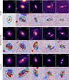 |
Fig. A.1. Examples of substructure detections using the optimal (black contours) and intrinsic (yellow contours) approaches. Galaxies are sorted from left to right by increasing redshift and split into three intrinsic substructure classes: clumps, moderately large, and extended (see Sect. 4.2). For each galaxy, we show the image (F277W for 1 < z < 2 and F444W for z > 2) and its residuals below. Red pixels correspond to positive residuals and blue pixels to negative ones. The scale of the residuals is set to ±2σ, with σ the local background fluctuations. In each image, we show the PSF FWHM at the bottom right and upper limits on the area of substructure classes as gray squares at the top right. The residuals show the detection area, highlighted with a thick green contour. |
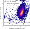 |
Fig. A.2. Density plot of the original area available for substructure detection versus the global effective radius of galaxies (low density in blue, high density in yellow; see Eq. 6 of Mercier et al. 2022 for a definition). We represent the area associated with the removed bulge as a dashed line, while the continuous line indicates the threshold used for the intrinsic substructure detection. |
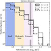 |
Fig. A.3. Distribution of substructures detected with the intrinsic method (see Sect. 3.3)by area, for three redshift bins: 1 < z < 2 (continuous line), 2 ≤ z < 3 (dotted line), and 3 ≤ z < 4 (dashed line). Vertical lines represent the 99% quantile for each distribution. Background colors indicate the area bins used in the analysis: clumps (blue, 1.3 < S/kpc2 < 4), moderately large substructures (orange, 4 < S/kpc2 < 13), and extended ones (pink, 13 < S/kpc2 < 40). |
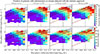 |
Fig. A.4. As in Fig. 2, but using stellar mass and SFR values from CIGALE. We do not show bins with fewer than ten galaxies. The presence or absence of certain bins with respect to Fig. 2 is driven by the differences in stellar mass and SFR between LEPHARE and CIGALE. All lines are defined similar to Fig. 2. This confirms that our results are unaffected by the SED fitting tool or assumptions. |
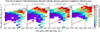 |
Fig. A.5. Same as the first row of Fig. 2 but weighting each galaxy by its detection area when computing, in each bin, the average fraction of galaxies with at least one substructure detected with the intrinsic approach. All lines are defined similar to Fig. 2. This shows that our results are not impacted by the detection area of substructures. The same applies to clumps. |
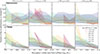 |
Fig. A.6. Fraction of rest-frame NIR flux in substructures (top row) and clumps (bottom row) as a function of the host galaxy’s stellar mass in four redshift bins, each bin spanning 1 Gyr of cosmic history. Galaxies are split in different bins of SFR, as illustrated with the various colored lines. The shaded areas correspond to the 16th and 84th percentiles for each SFR bin. See Fig. 3 for an alternative representation. |
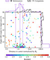 |
Fig. A.7. Figure similar to Fig. 7 but with the distance to the center of the host galaxy normalized by the disk scale length (Rd) derived with SEXTRACTOR++ on the four JWST/NIRCam bands. The vertical dashed lines correspond to the 16th and 84th percentiles of the distribution. |
Appendix B: Details on substructure detection
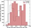 |
Fig. B.1. Histogram of the faintest detectable substructure in each galaxy. We split between galaxies for which the detection was carried out in the JWST/NIRCam F277W band (1 < z < 2; filled in red) and in the F444W band (2 ≤ z < 4; black dotted line). Vertical lines represent the 5% quartiles for the two bands, that is the values such that 95% of the galaxies have a lower detection threshold. We note that one must add 3.25 mag (or equivalently divide the corresponding flux threshold by 20) to convert these values into the detection threshold applied on each pixel. |
To determine whether 2σ is sufficient for the optimal detection (as in previous works; e.g., 5σ in Kalita et al. 2024 or 4.5σ in Kalita et al. 2025a), we performed a purity test. For each galaxy, we estimated iteratively the number n of σ that is required to not detect any structure in the background pixels13. We find a mean value of n = 1.4, a median value of n = 1.5, with the first quartile at n = 1.3, the third quartile at n = 1.6, and the 99% quantile at n = 2.1. Thus, we adopted a 2σ flux threshold. The primary reason for the threshold difference, compared to Kalita et al. (2024, 2025a), is likely their exclusion of substructures, which results in higher thresholds to isolate bright clumps located on top of fainter but more extended substructures.
Figure B.1 shows the histogram of the faintest detectable substructures for the entire sample. The histogram distinguishes galaxies at 1 < z < 2 (red; detection in F277W) and at 2 ≤ z < 4 (black dotted line; detection in F444W). As expected, the detections in F277W (the deepest band, see Casey et al. 2023) are slightly deeper than in F444W band with the 5% quantile (i.e., 95% of the galaxies have a lower threshold) at 28.85 mag in F444W and at 28.95 mag in F277W.
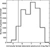 |
Fig. B.2. Histogram of the intrinsically faintest detectable substructure in each galaxy. The intrinsic flux threshold is computed for a substructure of 20 pixels with a 2σ detection per pixel, with σ measured from the local background around each galaxy (see Sect. 3.2), multiplied by 4πDL2/(1 + z) to take out the redshift dependence of the flux density. The vertical line marks the 5% quartile of the distribution, that is the value such that 95% of the galaxies have an intrinsic flux detection threshold that is higher than this value. |
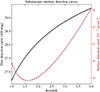 |
Fig. B.3. Flux and surface detection curves derived in Sect. 3.3 to select substructures with flux and area values that are above thresholds independent of redshift. The black continuous line represents the flux detection curve and the dashed red line represents the surface detection curve. Similar to Fig. B.1, one needs to add 3.25 mag to this curve to obtain the flux detection curve applied to each pixel individually during the substructure detection process. |
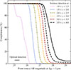 |
Fig. B.4. Completeness of the substructure detection for point sources in the optimal detection case (black solid line) and intrinsic detection case (dashed lines) in various redshift ranges. For each curve and magnitude bin, the completeness is estimated by injecting 500 PSF-convolved point sources in background-dominated regions around randomly sampled galaxies. |
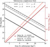 |
Fig. B.5. Link between the faintest observable magnitude (left vertical axis and black lines) or lowest stellar mass (right vertical axis and red lines) for the intrinsic detection method and the area of substructures. The stellar mass is evaluated at z = 1.5 and is expected to increase by 0.2 dex at z = 4. We estimate it, first, using the best-fit relationship between specific luminosity at a rest-frame wavelength of 1 μm and stellar mass for the entire COSMOS-Web sample (dark red line) and, second, using the best-fit relationship from Kalita et al. (2025b) for clumps in star-forming galaxies at z ≈ 1.5 detected in rest-frame optical (salmon-colored line). |
Appendix C: Weighted fraction of galaxies with substructures
C.1. Probability of substructure association with a galaxy
In some cases, detected substructures in residual maps lie between two or more galaxies, making it difficult to associate them to one or the other. Instead, we implement a weighting scheme for such cases when computing the fraction of galaxies with one or more substructures, as follows. For each galaxy, we loop through its substructures and search for nearby galaxies within a circular radius of 6 arcsec. This corresponds to the size of the cutouts used to detect substructures and we find that it is sufficient to detect nearby companions to the main galaxy. Assume N galaxies Gi are detected for substructure s. Each galaxy is separated by an angle θi from the substructure. To determine the angular separation, we use the center of the galaxies as well as the median right ascension and declination of the substructures as derived from their segmentation map. For each galaxy Gi, we must associate a probability Pr{s ∈ Gi} that the substructure s belongs to it. We define this probability as:
 (C.1)
(C.1)
 (C.2)
(C.2)
Equation C.1 states that a substructure twice as close to a galaxy should have double the probability. Furthermore, Eq. C.2 states that a substructure must belong to one of the galaxies. To determine the probability Pr{s ∈ Gk}, we isolate it from Eqs. C.2 and Eq. C.1:
![Mathematical equation: $$ \begin{aligned} \mathrm{Pr}\{s \in G_k\} = \left[ \sum _{i = 1}^N \theta _k / \theta _i \right]^{-1}, \end{aligned} $$](/articles/aa/full_html/2026/02/aa55981-25/aa55981-25-eq46.gif) (C.3)
(C.3)
at which point Eq. C.1 can be used to quickly calculate all other probabilities.
C.2. Probability of a galaxy having at least one substructure
What focus on the probability that a galaxy hosts at least one substructure14. Let Ns be the number of substructures in a galaxy. The probability of interest therefore writes Pr{Ns ≥ 1} = 1 − Pr{Ns = 0}. Assume that a galaxy G has N detected substructures si each with a probability Pr{si ∈ G}. Pr{Ns = 0} means that the galaxy has no substructures, that is that all si do not belong to G:
 (C.4)
(C.4)
where ∧ is the logical conjunction. Whether a substructure belongs to G should not affect other substructures. In other words, we assume all si independent, thus simplifying Eq. C.4 to a product of Pr{si ∉ G} = 1 − Pr{si ∈ G}, yielding:
![Mathematical equation: $$ \begin{aligned} \mathrm{Pr}\{N_s \ge 1\} = 1 - \prod _{i = 1}^N \left[ 1 - \mathrm{Pr}\{s_i \in G\} \right]. \end{aligned} $$](/articles/aa/full_html/2026/02/aa55981-25/aa55981-25-eq48.gif) (C.5)
(C.5)
C.3. Probability of a galaxy having at least n substructures
Another useful probability is Pr{Ns ≥ n}:
 (C.6)
(C.6)
Alternatively, it can be written down in terms of Pr{Ns ≥ n − 1}−Pr{Ns = n − 1} and solved recursively, but that requires calculating the same Pr{Ns = k} terms. The condition Ns = k requires computing the union of combinations of k substructures in G, and of N − k ones not in G. Let 𝒮 = {si} be the set of N substructures and (𝒮,k) the set of k-combinations of 𝒮. This yields:
![Mathematical equation: $$ \begin{aligned} \mathrm{Pr}\{N_s = k\} = \mathrm{Pr}\Bigg \{\underset {\mathcal{L} \in (\mathcal{S} , k)} {\bigvee} \left[ \underset {s \in \mathcal{L} } {\bigwedge} s \in G \underset {s \in \mathcal{S} \backslash \mathcal{L} }{\bigwedge} s \notin G \right]\Bigg \}, \end{aligned} $$](/articles/aa/full_html/2026/02/aa55981-25/aa55981-25-eq50.gif) (C.7)
(C.7)
where ∨ is the logical disjunction and 𝒮 ∖ ℒ is the set difference. Assuming independence of all si, this simplifies to
![Mathematical equation: $$ \begin{aligned} \mathrm{Pr}\{N_s = k\} = \sum _{\mathcal{L} \in (\mathcal{S} , k)} \left[ \prod _{s \in \mathcal{L} } \mathrm{Pr}\{s \in G\} \prod _{s \in \mathcal{S} \backslash \mathcal{L} } \left( 1 - \mathrm{Pr}\{s \in G\} \right) \right]. \end{aligned} $$](/articles/aa/full_html/2026/02/aa55981-25/aa55981-25-eq51.gif) (C.8)
(C.8)
Equations. C.6 and C.8 allow computing the probability that a galaxy has a given number of substructures or more. For example, setting n = 1 in Eq. C.6 recovers Eq. C.5.
Appendix D: Fraction of clumpy galaxies estimated from simulations
To compare our clumpy galaxy fraction measurements, we use results from the simulations studied in Mandelker et al. (2017). In their Fig. 16, they provide estimates of the fraction of clumpy galaxies and their uncertainties in three bins of stellar mass and various bins of redshift. Given a set 𝒮 of galaxies, where each galaxy Gi has a probability Pr{Nc, i ≥ 1} of hosting one or more clump, the fraction of clumpy galaxies is:
 (D.1)
(D.1)
where |𝒮| is the cardinality of the set. Mandelker et al. (2017) provides multiple fractions, fc(𝒮i), where each 𝒮i is a stellar mass subset of 𝒮, with ∀i, j, Si ∩ 𝒮j = ∅. Thus, we split the sum in Eq. D.1 into nested sums:
 (D.2)
(D.2)
where the sum is taken over all the stellar mass subsets of 𝒮. Using Eq. D.2, we estimate the fraction of clumpy galaxies in Mandelker et al. (2017) for 0.5-wide redshift bins for a population of galaxies with a similar stellar mass distribution as our sample. For z > 2.25, Mandelker et al. (2017) do not provide measurements for the most massive galaxies. Therefore, in this redshift range, we extrapolate the fractions using values for 9.8 < log10(M★/M⊙) < 10.6 and add 0.25 to each fraction, which corresponds to the typical difference between these two stellar mass ranges observed at lower redshift. Similarly, we assume an uncertainty of 0.25 at z > 2.25 and 10.6 < log10(M★/M⊙) < 11.1.
All Tables
Differences in stellar mass and star formation rate between CIGALE and LEPHARE for galaxies in the sample.
Fraction of galaxies with at least one substructure detected at a rest-frame wavelength of 1 μm as a function of redshift.
Linear correlation between the fraction of rest-frame NIR flux in substructures or clumps and the sSFR and partial correlation between the flux fraction and (i) the stellar mass of the host galaxy at a fixed host’s SFR, and (ii) the SFR of the host galaxy at a fixed host’s stellar mass.
All Figures
|
Fig. 1. Detection of substructures at a rest-frame wavelength of 1 μm for the entire sample (black) and for three substructure types: clumps (blue), moderately large ones (orange), and extended ones (pink). See Sect. 4.2 for more details. Left: fraction of galaxies with at least one substructure detected with the optimal approach (see Sect. 3.2) as a function of redshift. We show the rest-frame NIR detections carried out by Kalita et al. (2024) (red dashed line) and those in the rest-frame UV by Sattari et al. (2023) (green line and crosses). Middle: same but for the intrinsic detection approach (see Sect. 3.3). We show as a light red line a comparable 2σ detection (kp = 2, see reference) carried out in the rest-frame UV from Ribeiro et al. (2017) and, as a light green line, estimated fractions from the simulations studied in Mandelker et al. (2017, see Appendix D). In both figures on the left-hand side and in the middle, for each sample, we show uncertainties (16th and 84th percentiles) as shaded areas with similar colors. Right: median fraction of flux in substructures as a function of redshift for galaxies with at least one substructure. The uncertainties are shown with a blue shaded area for clumps, a double-dashed orange area for moderately large substructures, a single-dashed pink area for extended substructures, and a black shaded area for the entire sample. |
| In the text | |
|
Fig. 2. Top row: Median fraction of galaxies with at least one substructure detected with the intrinsic approach as a function of their host galaxy’s stellar mass and SFR in four redshift bins, each spanning roughly 1 Gyr of cosmic time. Bottom row: Same for clumps. Violet corresponds to 0% and red to 100% for substructures (70% for clumps). In each panel, the dashed line isolates the region where no substructure is detected (see Eq. (4)). Galaxies above the blue line are located in the starburst region, those in the hatched region are on the MS from Schreiber et al. (2015) evaluated at the average redshift of each panel, and those below the red line are in the red sequence with sSFR < 10−11 yr−1. We do not show bins with fewer than ten galaxies. |
| In the text | |
|
Fig. 3. Same as Fig. 2 but representing the fraction of flux in substructures (top row) or clumps (bottom row) detected using the intrinsic detection approach in each galaxy host’s stellar mass and SFR bin. To compute the fraction of flux we consider only those galaxies that contain at least one substructure. |
| In the text | |
|
Fig. 4. Evolution of the fraction of galaxies with substructures (left panel) and clumps (middle panel) detected with the intrinsic detection approach as a function of redshift for different regions of the M★ − SFR plane, as illustrated in the right panel with circles of a different color, line style, and thickness. We use the same redshift bins spanning 1 Gyr of cosmic time as in Figs. 2 and 3. Each circular region has a radius of 0.2 dex and the regions are chosen to evenly map the plane. We only show regions with more than ten galaxies in all redshift bins and lines are slightly offset vertically to improve readability. |
| In the text | |
|
Fig. 5. Intrinsic detection of substructures (black) and clumps (blue) for galaxies on the MS (continuous lines) and for starbursts (dotted lines) as a function of redshift. For comparison, we also show the rest-frame UV detections from Ribeiro et al. (2017, light red). Shaded areas correspond to the uncertainties computed as the 16th and 84th percentiles. |
| In the text | |
|
Fig. 6. Average probability that a galaxy of a given stellar mass with at least one clump hosts either a single clump (continuous lines) or two or more clumps (dashed lines) for starbursts (blue circles), galaxies on the MS (black squares), in the green valley (green diamonds), and in the red sequence (red crosses). For each class, we show the standard deviation of the probability as a semitransparent filled area with a similar color. The probabilities are computed using Eqs. (C.6) and (C.8). |
| In the text | |
|
Fig. 7. Position of intrinsic substructures (circles) with respect to the galaxy host color-coded with redshift. The detection is done in edge-on galaxies with bulges contributing less than 50% to the rest-frame NIR flux. We show on the x axis the distance to the center of the host galaxy and, on the y axis, the angle between the barycenter of the substructure and the major axis of the host galaxy. Crosses show the distribution of galaxy companions with properties comparable to clumps, selected at a distance below 3 arcsec from the galaxy, with a total flux in the rest-frame NIR below 15%, and within 1σ of the redshift of the main galaxy. Pink dotted lines represent isocontours of the vertical distance to the galaxy plane. |
| In the text | |
|
Fig. A.1. Examples of substructure detections using the optimal (black contours) and intrinsic (yellow contours) approaches. Galaxies are sorted from left to right by increasing redshift and split into three intrinsic substructure classes: clumps, moderately large, and extended (see Sect. 4.2). For each galaxy, we show the image (F277W for 1 < z < 2 and F444W for z > 2) and its residuals below. Red pixels correspond to positive residuals and blue pixels to negative ones. The scale of the residuals is set to ±2σ, with σ the local background fluctuations. In each image, we show the PSF FWHM at the bottom right and upper limits on the area of substructure classes as gray squares at the top right. The residuals show the detection area, highlighted with a thick green contour. |
| In the text | |
|
Fig. A.2. Density plot of the original area available for substructure detection versus the global effective radius of galaxies (low density in blue, high density in yellow; see Eq. 6 of Mercier et al. 2022 for a definition). We represent the area associated with the removed bulge as a dashed line, while the continuous line indicates the threshold used for the intrinsic substructure detection. |
| In the text | |
|
Fig. A.3. Distribution of substructures detected with the intrinsic method (see Sect. 3.3)by area, for three redshift bins: 1 < z < 2 (continuous line), 2 ≤ z < 3 (dotted line), and 3 ≤ z < 4 (dashed line). Vertical lines represent the 99% quantile for each distribution. Background colors indicate the area bins used in the analysis: clumps (blue, 1.3 < S/kpc2 < 4), moderately large substructures (orange, 4 < S/kpc2 < 13), and extended ones (pink, 13 < S/kpc2 < 40). |
| In the text | |
|
Fig. A.4. As in Fig. 2, but using stellar mass and SFR values from CIGALE. We do not show bins with fewer than ten galaxies. The presence or absence of certain bins with respect to Fig. 2 is driven by the differences in stellar mass and SFR between LEPHARE and CIGALE. All lines are defined similar to Fig. 2. This confirms that our results are unaffected by the SED fitting tool or assumptions. |
| In the text | |
|
Fig. A.5. Same as the first row of Fig. 2 but weighting each galaxy by its detection area when computing, in each bin, the average fraction of galaxies with at least one substructure detected with the intrinsic approach. All lines are defined similar to Fig. 2. This shows that our results are not impacted by the detection area of substructures. The same applies to clumps. |
| In the text | |
|
Fig. A.6. Fraction of rest-frame NIR flux in substructures (top row) and clumps (bottom row) as a function of the host galaxy’s stellar mass in four redshift bins, each bin spanning 1 Gyr of cosmic history. Galaxies are split in different bins of SFR, as illustrated with the various colored lines. The shaded areas correspond to the 16th and 84th percentiles for each SFR bin. See Fig. 3 for an alternative representation. |
| In the text | |
|
Fig. A.7. Figure similar to Fig. 7 but with the distance to the center of the host galaxy normalized by the disk scale length (Rd) derived with SEXTRACTOR++ on the four JWST/NIRCam bands. The vertical dashed lines correspond to the 16th and 84th percentiles of the distribution. |
| In the text | |
|
Fig. B.1. Histogram of the faintest detectable substructure in each galaxy. We split between galaxies for which the detection was carried out in the JWST/NIRCam F277W band (1 < z < 2; filled in red) and in the F444W band (2 ≤ z < 4; black dotted line). Vertical lines represent the 5% quartiles for the two bands, that is the values such that 95% of the galaxies have a lower detection threshold. We note that one must add 3.25 mag (or equivalently divide the corresponding flux threshold by 20) to convert these values into the detection threshold applied on each pixel. |
| In the text | |
|
Fig. B.2. Histogram of the intrinsically faintest detectable substructure in each galaxy. The intrinsic flux threshold is computed for a substructure of 20 pixels with a 2σ detection per pixel, with σ measured from the local background around each galaxy (see Sect. 3.2), multiplied by 4πDL2/(1 + z) to take out the redshift dependence of the flux density. The vertical line marks the 5% quartile of the distribution, that is the value such that 95% of the galaxies have an intrinsic flux detection threshold that is higher than this value. |
| In the text | |
|
Fig. B.3. Flux and surface detection curves derived in Sect. 3.3 to select substructures with flux and area values that are above thresholds independent of redshift. The black continuous line represents the flux detection curve and the dashed red line represents the surface detection curve. Similar to Fig. B.1, one needs to add 3.25 mag to this curve to obtain the flux detection curve applied to each pixel individually during the substructure detection process. |
| In the text | |
|
Fig. B.4. Completeness of the substructure detection for point sources in the optimal detection case (black solid line) and intrinsic detection case (dashed lines) in various redshift ranges. For each curve and magnitude bin, the completeness is estimated by injecting 500 PSF-convolved point sources in background-dominated regions around randomly sampled galaxies. |
| In the text | |
|
Fig. B.5. Link between the faintest observable magnitude (left vertical axis and black lines) or lowest stellar mass (right vertical axis and red lines) for the intrinsic detection method and the area of substructures. The stellar mass is evaluated at z = 1.5 and is expected to increase by 0.2 dex at z = 4. We estimate it, first, using the best-fit relationship between specific luminosity at a rest-frame wavelength of 1 μm and stellar mass for the entire COSMOS-Web sample (dark red line) and, second, using the best-fit relationship from Kalita et al. (2025b) for clumps in star-forming galaxies at z ≈ 1.5 detected in rest-frame optical (salmon-colored line). |
| In the text | |
Current usage metrics show cumulative count of Article Views (full-text article views including HTML views, PDF and ePub downloads, according to the available data) and Abstracts Views on Vision4Press platform.
Data correspond to usage on the plateform after 2015. The current usage metrics is available 48-96 hours after online publication and is updated daily on week days.
Initial download of the metrics may take a while.